Solving linear systems (6 lectures)

Transcription

1 Chapter 2 Solving linear systems (6 lectures) 2.1 Solving linear systems: LU factorization (1 lectures) Reference: [Trefethen, Bau III] Lecture 20, 21 How do you solve Ax = b? (2.1.1) In numerical linear algebra, NEVER compute A 1 then A 1 b. Reason: very expensive! storage! less accurate! Gaussian elimination Basic idea: Example 1 (Gaussian elimination). Solve x 1 x 2 x 3 2 = 1. (2.1.2) 0

2 Gaussian elimination is the same as This gives rise to LU factorization = (2.1.3) x 1 x 2 x 3 x 1 x 2 x }{{}}{{} L U = 1 3 (2.1.4) 1 x 1 x 2 x 3 2 = 1 (2.1.5) 0 LUx = b (2.1.6) Solution: x 1 x 2 x 3 2 = 1 (2.1.7) LU factorization, forward/backward substitutions Exact solver (Gaussian elimination) of Ax = b is equivalent to: LU-factorize the matrix A: A = LU Solve Ly = b for intermediate solution y (forward substitution) Solve Ux = y for final solution x (backward substitution) We can derive the LU factorization based on the process of Gaussian elimination, as follows: 20

3 Algorithm 1 LU factorization 1: for k = 1,, n 1 do iterate over all rows 2: for i = k + 1,, n do iterate over all rows beneath row k 3: mult = a ik /a kk determine the multiplicative factor of row i (i > k) 4: a ik = mult form the k-th column of the lower triangular matrix 5: for j = k + 1,, n do iterate over all columns in a row 6: a ij = a ij mult a kj subtract the scaled row data and form the i-th row of the upper triangular matrix 7: end for 8: end for 9: end for Theorem 1 (LU factorization). A = LU, (2.1.8) where L= lower triangular matrix, unit diagonal; U= upper triangular matrix. In addition, 1 A (n-1) = mult U L= mult 1 We can also derive the forward substitution based on the process of Gaussian elimination, as follows: Algorithm 2 Forward substitution for Ly = b 1: for i = 1,, n do iterate over all rows 2: y i = b i 3: for j = 1,, i 1 do iterate over all (lower-triangular) columns in a row 4: y i = y i l ij y j solve for y i 5: end for 6: y i = y i /l ii skip this line if l ii = 1 7: end for 21

4 Exercise 1 (backward substitutions). Write down the algorithm for the backward substitution Ux = y Complexity Evaluate complexity by the number of FLOPs (floating point operations): +,,,. The complexity of LU factorization: From Algorithm 1, we have n 1 n n n 1 n n 1 2 = 2 (n i) = 2 (n i) 2 = 2 3 n3 + O(n 2 ), (2.1.9) i=1 k=i+1 j=i+1 i=1 i=1 k=i+1 where we have used n i = 1 n n(n + 1), 2 i=1 i=1 i 2 = 1 n(n + 1)(2n + 1). (2.1.10) 6 Exercise 2 (Forward/backward substitutions). Analyze the complexity of the forward substitution Ly = b and the backward substitution Ux = y. The overall complexity of the exact solver: 2 3 n3 + O(n 2 ). (2.1.11) Pivoting Example 2 (Instability of Gaussian elimination when a 11 = 0). Consider solving x x 2 = 6. (2.1.12) Since the pivot a 11 = 0, we cannot perform LU factorization! Example 3 (Partial pivoting). The solution for the instability issue is pivoting. Reorder the equations (the rows of A and the right hand side b), such that the largest among a i1 (i = 1, 2, 3) becomes the pivot x x 2 = 6. (2.1.13) x 3 x 3 22

5 x x 2 = (2.1.14) x 3 Next we perform Gaussian elimination on the red submatrix, which requires another pivoting! x x 2 = 1. (2.1.15) x Example 4 (Complete pivoting). Instead, reorder both the equations (the rows of A and b) and the unknowns (the columns of A and x), such that the largest among a ij (i = 1, 2, 3; j = 1, 2, 3) becomes the pivot. Remark 1 (Reordering) x 1 x 2 x 3 x 3 x 2 x 1 = Reordering the equations = reordering the rows of A and b (2.1.16) 8 6 = 1. (2.1.17) 8 Reordering the unknowns = reordering the columns of A and x. In general, after the (k 1)-th Gaussian elimination done a (k-1) kk 0 A (k-1) row k if the original pivot a (k 1) kk = 0 or a (k 1) kk 0, then pivoting is required. 23

6 Two possible pivoting strategies: Complete pivoting: Search the largest (absolute value) element in A (k 1), and pivot. Partial pivoting: Search the largest (absolute value) element in the column k of A (k 1), and pivot. In practice, we use partial pivoting, since complete pivoting is expensive, and does not yield much more gains! To summarize the essence of Gaussian elimination with partial pivoting: to: Exact solver (Gaussian elimination) of Ax = b with partial pivoting is equivalent Permutation of the rows of A: A P matrix = P A, where P is a certain permutation LU-factorize the matrix A P : A P = LU Solve Ly = b for intermediate solution y (forward substitution) Solve Ux = y for final solution x (backward substitution) Example 5 (Permutation matrix for partial pivoting). In Example 3, the permutation matrix is given by: 1 P = P 2 P 1 = = (2.1.18) The algorithm of LU factorization with partial pivoting is given as follows: 24

7 Algorithm 3 LU factorization with partial pivoting 1: for k = 1,, n 1 do iterate over all rows 2: Select i = arg max i k a ik 3: a k,k:m a i,k:m interchange row k and row i (upper triangular part) 4: a k,1:k 1 a i,1:k 1 interchange row k and row i (lower triangular part) 5: for i = k + 1,, n do iterate over all rows beneath row k 6: mult = a ik /a kk determine the multiplicative factor of row i (i > k) 7: a ik = mult form the k-th column of the lower triangular matrix 8: for j = k + 1,, n do iterate over all columns in a row 9: a ij = a ij mult a kj subtract the scaled row data and form the i-th row of the upper triangular matrix 10: end for 11: end for 12: end for When is pivoting unnecessary? However, in some situations, we can prove that pivoting is unnecessary. The following condition on A will ensure pivoting is not necessary and the LU factorization is always stable: A is symmetric positive definite (SPD), A is row diagonally dominant, or A is column diagonally dominant. Here we show that pivoting is unnecessary for SPD matrices. A quick review on SPD matrices can be found in the supplementary notes. Theorem 2 (Pivoting being unnecessary for SPD matrices). Suppose A is SPD. Then during Gaussian elimination, a (k 1) kk > 0. Proof. For simplicity, consider k = 1. Suppose ( A = 25 a 11 v v T B ) (2.1.19)

8 is SPD. Here a 11 is a number, v R n 1 and B R (n 1) (n 1). Then a 11 > 0. Now eliminate v using a 11 as pivot: ( ) ( ) a 11 v T a11 v T (2.1.20) v B 0 B vvt a 11 Hence the Gaussian elimination gives A (1) = B vvt a 11. (2.1.21) Next we will prove that A (1) is SPD. It is easy to see that A (1) is symmetric, so our focus is to prove that A (1) is PD. Let x R n 1 and ( ) y xt v a 11 R n (2.1.22) x Some straightforward algebra can show that y T Ay = x T ( Since A is PD, we have B vvt a 11 ) x = x T A (1) x. (2.1.23) y T Ay > 0 x T A (1) x > 0. (2.1.24) Hence, A (1) is PD. Then a (1) 22 > 0. k > 1 can be proved by in the same fashion (induction). Remark 2. You will prove that pivoting is unnecessary for row/column diagonally dominant matrices in your assignment. 26

9 2.2 Solving symmetric positive definite systems: Cholesky factorization (1 lectures) Reference: [Trefethen, Bau III] Lecture 23 The complexity of LU factorization is 2 3 n3, which is still very expensive! Consider a image. The dimension of the resulting linear system is n = The computational complexity is 10 18! Consider special linear systems: Exploit the special structure of linear systems More efficient LU factorization We will see in this lecture that Generic matrix: LU factorization = LDM T factorization. Symmetric matrix: LDL T factorization. Positive definite matrix: LDM T factorization, where D > 0. Symmetric positive definite matrix: LDL T factorization, where D > 0 Cholesky factorization (A = GG T ) Generic matrix: LDM T factorization Theorem 3 (LDM T factorization). If all the leading principal submatrices of A are nonsingular, then there exists unique unit lower triangular matrices L and M, and a unique diagonal matrix D, such that A = LDM T. (2.2.1) Proof. A = LU = LDD 1 U = LDM T, (2.2.2) where D is the diagonal part of U and M T = D 1 U (rescale each row such that it is unit diagonal). Remark 3. LDM T factorization is simply a variant of LU factorization. Nothing new! 27

10 2.2.2 Symmetric matrix: LDL T factorization Theorem 4 (LDL T factorization). If A is symmetric, then M = L, or equivalently, A = LDL T. (2.2.3) Proof. A = LDM T M 1 AM T = M 1 LDM T M T = M 1 LD Note that M 1 AM T is symmetric M 1 LD is symmetric. Note that both M and L are unit lower triangular M 1 L is unit lower triangular (why?) M 1 LD is lower triangular. Hence, M 1 LD is a diagonal matrix! M 1 L is a diagonal matrix! Note that M 1 L is unit lower triangular M 1 L is an identity matrix! M = L. Remark 4. Why matters? Save half the work by computing L and D only Positive definite (PD) matrix: LDM T factorization, where D > 0 Theorem 5 (LDM T factorization for PD). If A is PD, then for A = LDM T, D > 0. Proof. A = LDM T L 1 AL T = L 1 LDM T L T = DM T L T Note that L 1 AL T is PD DM T L T is PD. By Corollary 8, diag(dm T L T ) > 0. Note that both M and L are unit lower triangular M T L T is unit upper triangular (why?) diag(dm T L T ) = D. Hence, D > Symmetric positive definite (SPD) matrix: Cholesky factorization Symmetric matrix: PD matrix: A = LDM T M = L. (2.2.4) A = LDM T D > 0. (2.2.5) 28

11 Then SPD matrix: A = LDM T M = L, D > 0. (2.2.6) Rewrite: A = LDL T = LD 1 2 D 1 2 L T = (LD 1 2 )(LD 1 2 ) T = GG T. (2.2.7) This gives rise to Cholesky factorization where G is lower triangular. A = GG T, (2.2.8) Cholesky factorization algorithm Naively, LU factorization, and go through the process above Cholesky. But can we do Cholesky directly? The answer is yes! We can verify that ( α A = v If A is SPD, then B vvt α ) ( α ) ( v T 0 = B I v α I 0 0 B vvt α is SPD (exercise). Let ) ( α ) v T α. (2.2.9) 0 I B vvt α = G 1G T 1. (2.2.10) Then ( α ) ( α ) 0 v T A = α v = GG α G T. (2.2.11) 1 0 G T 1 This implies that we can perform Cholesky factorization recursively. Exercise 3. Prove that B vvt α is SPD. Hint: Check XT AX, where X ( ) 1 vt α. (2.2.12) 0 I You should get X T AX = ( ) α 0. (2.2.13) 0 B vvt α 29

12 Example 6 (Cholesky factorization). Based on (2.2.9), Cholesky factorize the following 3 3 matrix: A = (2.2.14) The answer is To summarize the Choleksy factorization: Algorithm 4 Cholesky factorization 3 G = 1 2 (2.2.15) : for k = 1,, n do Iterate from top to bottom along diagonal. 2: a kk = a kk Factor the diagonal element α. 3: for i = k + 1,, n do 4: a ik = a ik /a kk Update current column entries below the diagonal v = v/ α. 5: end for 6: for j = k + 1,, n do 7: for i = j,, n do 8: a ij = a ij a ik a jk Update the lower right block B = B vv T /α (below the diagonal only). 9: end for 10: end for 11: end for Complexity: The complexity of the Cholesky factorization is n O(n2 ). (2.2.16) Exercise 4. Verify the complexity. Remark 5. In order to solve Ax = b, after the Cholesky factorization A = GG T, we use forward/backward substitution to solve GG T x = b. 30

13 2.3 From partial differential equations to sparse linear systems (1 lectures) Reference: [Saad] Partial differential equations (PDEs) Three most basic linear partial differential equations (PDEs). t: time. x, y: space. Wave equation: Solution: Figure: u t + au x = 0, u(x, 0) = sin(2πx). (2.3.1) u(x, t) = sin(2π(x at)). (2.3.2) Heat equation: Solution: u t σu xx = 0, u(x, 0) = sin(kπx), u(0, t) = 0, u(1, t) = 0. k is an integer, (2.3.3) u(t, x) = e k2 π 2 σt sin(kπx). (2.3.4) 31

14 Figure: Poisson equation: u xx + u yy = 2π 2 sin(πx) sin(πy), inside (0, 1) (0, 1), u = 0, on the boundary of [0, 1] [0, 1]. (2.3.5) Solution: Figure: u(x, y) = sin(πx) sin(πy). (2.3.6) Remark 6. In this course, we only discuss time-independent problems (boundary problems, steady state problems). Time dependent problems, or more generally, numerical techniques for all types of PDEs, AMATH 342, AMATH 442, AMATH 741 / CS 778. Remark 7. In general, difficult to find analytical solutions. Need numerical solutions! 32

15 D Poisson equation Consider solving steady heat distribution or electric potential on a line: u xx (x) = f(x), inside (0, 1), (2.3.7) u(0) = a, u(1) = b. (2.3.8) Idea: Continuous Discrete. Discretize the computational domain [0, 1] into a square grid. Find u(x) at each grid point. Finite difference discretization. Construct a grid: gives Grid size: m = 4 Grid spacing: h = 1 m+1 = 1 5. Grid coordinates: x 0 = 0, x 1 = 1 5, x 2 = 2 5, x 3 = 3 5, x 4 = 4 5, x 5 = 1. Right hand side: f(x 0 ), f(x 1 ), f(x 2 ), f(x 3 ), f(x 4 ), f(x 5 ), denoted as f 0, f 1, f 2, f 3, f 4, f 5. Our goal: Solve for the unknowns u(x 0 ), u(x 1 ), u(x 2 ), u(x 3 ), u(x 4 ), u(x 5 ), denoted as u 0, u 1, u 2, u 3, u 4, u 5. On the boundary, Equation (2.3.8) Inside 0 < x < 1, check Equation (2.3.7). u(0) = a, u(1) = b. (2.3.9) u 0 = a, u 5 = b. (2.3.10) 33

16 The 2nd derivative: On the grid, approximate it by u xx (x) = lim h 0 u(x h) 2u(x) + u(x + h) h 2. (2.3.11) u xx (x i ) u(x i h) 2u(x) + u(x i + h) h 2 = u i 1 2u i + u i+1 h 2, i = 1, 2, 3, 4. (2.3.12) Equation (2.3.7) becomes i = 1: Note that u 0 = a: i = 2: i = 3: i = 4: Note that u 5 = b: u xx (x) = f(x), inside (0, 1), (2.3.13) u i 1 + 2u i u i+1 h 2 = f i, i = 1, 2, 3, 4. (2.3.14) u 0 + 2u 1 u 2 h 2 = f 1, 2u 1 u 2 h 2 = f 1 + a h 2, u 1 + 2u 2 u 3 h 2 = f 2, u 2 + 2u 3 u 4 h 2 = f 3, u 3 + 2u 4 u 5 h 2 = f 4. u 3 + 2u 4 h 2 = f 4 + b h 2. 34

17 Align the unknowns: 2 h 2 u 1 1 h 2 u 2 = f 1 + a h 2, 1 h 2 u h 2 u 2 1 h 2 u 3 = f 2, 1 h 2 u h 2 u 3 1 h 2 u 4 = f 3, This gives a linear system: h h 2 u h 2 u 4 = f 4 + b h 2. u 1 u 2 u 3 u 4 (2.3.15) f 1 + a h 2 = f 2 f 3. (2.3.16) f 4 + b h 2 For general m, the discretization of Equation (2.3.7) gives rise to a linear system where the pattern is A = h , u = Au = f, (2.3.17) u 1 u 2 u 3. u m 1 u m Remark 8. The matrix A is SPD (see supplementary notes). Algorithm 5 1D discrete Laplacian 1: for i = 1,, n do 2: A i,i = 2/h 2 3: if i > 1 then 4: A i,i 1 = 1/h 2 5: end if 6: if i < m then 7: A i,i+1 = 1/h 2 8: end if 9: end for f 1 + a h 2 f 2 f 3, f =.. f m 1 f m + b h 2 (2.3.18) 35

18 D Poisson equation Consider solving steady heat distribution or electric potential in a squared box: u xx u yy = f, inside (0, 1) (0, 1), u = g, on the boundary of [0, 1] [0, 1]. (2.3.19) Idea: Continuous Discrete. Discretize the computational domain [0, 1] [0, 1] into a square grid. Find u(x, y) at each grid point (x, y). Finite difference discretization. Construct a grid: Grid size: m = 4 Grid spacing: h = 1 m+1 = 1 5. Grid coordinates (boundary excluded) (x 1, y 1 ), (x 1, y 2 ), (x 1, y 3 ), (x 1, y 4 ), (x 2, y 1 ), (x 2, y 2 ), (x 2, y 3 ), (x 2, y 4 ), (x 3, y 1 ), (x 3, y 2 ), (x 3, y 3 ), (x 3, y 4 ), (x 4, y 1 ), (x 4, y 2 ), (x 4, y 3 ), (x 4, y 4 ). (lexicographic order) Right hand side: f at these points, denoted as f 1,1, f 1,2,, f 4,4. Our goal: Solve for the unknowns u 1,1, u 1,2,, u 4,4. 36

19 Inside (0, 1) (0, 1), check Equation (2.3.19). The 2nd derivative: u xx (x, y) = lim h 0 u(x h, y) 2u(x, y) + u(x + h, y) h 2, (2.3.20) u yy (x, y) = lim h 0 u(x, y h) 2u(x, y) + u(x, y + h) h 2. (2.3.21) On the grid, approximate it by u xx (x i, y j ) u(x i h, y j ) 2u(x i, y j ) + u(x i + h, y j ) h 2 u yy (x i, y j ) u(x i, y j h) 2u(x i, y j ) + u(x i, y j + h) h 2 = u i 1,j 2u i,j + u i+1,j h 2, (2.3.22) = u i,j 1 2u i,j + u i,j+1 h 2. (2.3.23) PDE (2.3.19) can be approximated by u i 1,j + 2u i,j u i+1,j h 2 + u i,j 1 + 2u i,j u i,j+1 h 2 = f i,j, i, j = 1, 2, 3, 4. (2.3.24) 1 h 2 This gives a linear system: u 1,1 u 1,2 u 1,3 u 1,4 u 2,1 u 2,2 u 2,3 u 2,4 u 3,1 u 3,2 u 3,3 u 3,4 u 4,1 u 4,2 u 4,3 u 4,4 = f 1,1 +g 0,1 /h 2 +g 1,0 /h 2 f 1,2 +g 0,2 /h 2 f 1,3 +g 0,3 /h 2 f 1,4 +g 0,4 /h 2 +g 1,5 /h 2 f 2,1 +g 2,0 /h 2 f 2,2 f 2,3 f 2,4 +g 2,5 /h 2 f 3,1 +g 3,0 /h 2 f 3,2 f 3,3 f 3,4 +g 3,5 /h 2 f 4,1 +g 5,1 /h 2 +g 4,0 /h 2 f 4,2 +g 5,2 /h 2 f 4,3 +g 5,3 /h 2 f 4,4 +g 5,4 /h 2 +g 4,5 /h 2 (2.3.25) For general m, the discretization of Equation (2.3.7) gives rise to a linear system 37 Au = f, (2.3.26)

20 where the pattern is A = 1 h R m2 m 2. (2.3.27) For convenience, we write it into a block form: B 1 I A = 1 I B 2 I R m2 m 2, (2.3.28) h 2 I B m 1 I I B m where each block B i (i = 1,, m) reads B i = R m m. (2.3.29) Remark 9. By writing the matrix A in a block form, it becomes much easier to handle the boundary terms that are moved to the right hand side of the equation. Whenever a matrix entry falls outside a block or the full matrix, kill it (and move it to the right hand side). Remark 10. The matrix A is again, SPD (see supplementary notes). 38

21 Algorithm 6 2D discrete Laplacian 1: for i = 1,, m do 2: for j = 1,, m do 3: A m(i 1)+j, m(i 1)+j = 4/h 2 4: if i > 1 then 5: A m(i 1)+j, m(i 1 1)+j = 1/h 2 6: end if 7: if i < m then 8: A m(i 1)+j, m(i+1 1)+j = 1/h 2 9: end if 10: if j > 1 then 11: A m(i 1)+j, m(i 1)+j 1 = 1/h 2 12: end if 13: if j < m then 14: A m(i 1)+j, m(i 1)+j+1 = 1/h 2 15: end if 16: end for 17: end for Convection-diffusion equation Consider solving a steady state of the (fluid, gas) particles that allow diffusion and convection: u xx u yy + au x + bu y = f, inside (0, 1) (0, 1), u = g, on the boundary of [0, 1] [0, 1]. (2.3.30) In this case, we also need to consider approximating the first derivatives. Take u x (x, y) as example. There are three different possibilities: Central difference: u(x + h, y) u(x h, y) u x (x, y) = lim, (2.3.31) h 0 2h On the grid, approximate it by u x (x i, y j ) u(x i + h, y j ) u(x i h, y j ) 2h = u i+1,j u i 1,j. (2.3.32) 2h 39

22 Forward difference: u(x + h, y) u(x, y) u x (x, y) = lim, (2.3.33) h 0 h On the grid, approximate it by u x (x i, y j ) u(x i + h, y j ) u(x i, y j ) h = u i+1,j u i,j. (2.3.34) h Backward difference: u(x, y) u(x h, y) u x (x, y) = lim, (2.3.35) h 0 h On the grid, approximate it by u x (x i, y j ) u(x i, y j ) u(x i h, y j ) h = u i,j u i 1,j. (2.3.36) h For stability reasons, we choose forward/backward differences, depending on the signs of a and b. When a > 0 and b > 0, use backward differences for u x and u y. Hence, PDE (2.3.30) can be approximated by u i 1,j + 2u i,j u i+1,j h 2 This gives rise to a linear system + u i,j 1 + 2u i,j u i,j+1 +a u i,j u i 1,j +b u i,j u i,j 1 = f h 2 i,j. h h (2.3.37) Au = f, (2.3.38) where the full matrix is B 1 I A = 1 (1 + ah)i B 2 I , (2.3.39) h 2 (1 + ah)i B m 1 I (1 + ah)i B m 40

23 and the submatrices are 4 + ah + bh 1 (1 + bh) 4 + ah + bh 1 B i = (2.3.40) (1 + bh) 4 + ah + bh 1 (1 + bh) 4 + ah + bh Exercise 5. When a > 0, b < 0, for stability reason, we use backward difference for u x and forward difference for u y : u i 1,j + 2u i,j u i+1,j h 2 Write down the matrix A. + u i,j 1 + 2u i,j u i,j+1 +a u i,j u i 1,j +b u i+1,j u i,j = f h 2 i,j. h h (2.3.41) Remark 11. This course does not require you to know how to discretize the PDEs. It is a very complicated subject and research topic indeed! (AMATH 342, AMATH 442, AMATH 741 / CS 778). The requirement is that once a PDE expert tells you how to discretize the PDEs, you can write down the resulting linear system Au = f. In general, a discretization of partial differential equation gives rise to a band system, or more generally, a sparse linear system. 41

24 2.4 Solving sparse systems (2 lectures) Reference: [Saad] We have seen that PDE discretization gives rise to a sparse linear system, or more precisely, band linear system LU factorization of band systems A general form of band systems with upper bandwidth q and lower bandwidth p: A =. (2.4.1) Example 7 (Band system) A = (2.4.2) We have q = 1, p = 2. Example 8 (1D Poisson matrix). We have p = q = A = h (2.4.3)

25 Example 9 (2D Poisson matrix). A = 1 h (2.4.4) We have p = q = m (Note that the size of the matrix A is m 2 m 2 ). Theorem 6 (LU factorization of a band system). If A has upper bandwidth q and lower bandwidth p, then for A = LU, U has upper bandwidth q and L has lower bandwidth p. = Algorithm 7 LU factorization for band system 1: for k = 1,, n 1 do iterate over all rows 2: for i = k + 1,, min(k + p, n) do iterate over all rows beneath row k and above row min(k + p, n). 3: mult = a ik /a kk determine the multiplicative factor of row i 4: a ik = mult form the k-th column of the lower triangular matrix 5: for j = k + 1,, min(k + q, n) do iterate between the (k + 1)-th column and the min(k + q, n)-th column in a row 6: a ij = a ij mult a kj subtract the scaled row data and form the k-th row of the upper triangular matrix 7: end for 8: end for 9: end for 43

26 Complexity: If n p and n q, then the computational complexity 2npq. Exercise 6. Verify the complexity. Remark 12. Compared to 2 3 n3 for generic LU, band LU is much faster! Issues with sparse systems Band matrices are only special instances of sparse matrices. Consider more general sparse matrices. Something we can do: Usually a constant number of non-zeros per row, or O(n) non-zeros in total. O(n) storage of a sparse matrix: CRS (compressed row storage) In LU factorization, skip all the zero entries when computing However, there are still issues! Example 10 (Arrow matrix). Consider solving a ij = a ij a ik a kk a kj. (2.4.5) Ax = b, (2.4.6) where A is an arrow matrix: A = (2.4.7) The LU factorization of A: 1 1 = (2.4.8) 44

27 L and U are dense! Storage: O(n 2 ). Cost: O(n 3 ). Bad! However, if we reorder both the unknowns (the column of A) and the equations (the row of A): A P x P = b P (2.4.9) then 1 1 A P = = (2.4.10) Example 11 (2D Poisson matrix with m x < m y ). Consider Poisson matrix with m x < m y. Total number of grid points is n = m x m y. x-axis first, y-axis second: Band width is m x. Computational cost is O(m 2 xn). y-axis first, x-axis second: Band width is m y. Computational cost is O(m 2 yn). A sparse matrix A can still result in dense L and U. The ordering of the sparse matrix A can dramatically affect the sparsity of the resulting L and U Graph representation of matrices Our goal: reordering helps reducing storage and computational cost. Our tool: graph representation of matrices. A sparse matrix A can be represented by a graph. If a i,j 0, then there exists an edge from node i to j. 45

28 Example 12 (Graph representation). A = (2.4.11) Example 13 (Graph representation). Graph representation for 1D and 2D Poisson matrices: The graph of matrix with symmetric structure remains unchanged under reordering. The graph structure often has a physical or geometrical interpretation on the systems. What does Gaussian elimination do with the graph? Example 14 (Graph representation). 0 0 (2.4.12) 46

29 Gaussian elimination of the node i deletes node i and all the edges it connects, and creates new edge from j to k within the remaining subgraph if there is a fill-in at (j, k) Ordering algorithm (I): Cuthill-McKee ordering Idea: In each row, the fillings of L only occur between the first non-zero in the row and the diagonal. Keep the envelop as close to the diagonal as possible. Try to label the nodes such that the labels of the graph neighbors are as close as possible. 47

30 Algorithm 8 Cuthill-McKee ordering 1: Pick starting node 2: for i = 1,, n do 3: Find all unnumbered neighbors of node i 4: Label them in order of degree (smallest first) 5: end for 6: Reverse Cuthill-McKee: node i node n i+1, i = 1,, n. The reverse order is better! Example 15 (Cuthill-McKee ordering). 48

31 Example 16 (Cuthill-McKee ordering). Example 17 (Why reversed order is better?). CM ordering: 1-g, 2-h, 3-e, 4-b, 5-f, 6-c, 7-j, 8-a, 9-d, 10-i. RCM ordering: 1-i, 2-d, 3-a, 4-j, 5-c, 6-f, 7-b, 8-e, 9-h, 10-g. Example 18 (Why reversed order is better?). CM ordering: 1-A, 2-G, 3-B, 4-C, 5-D, 6-E, 7-F. Reversed CM ordering: 1-F, 2-E, 3-D, 4-C, 5-B, 6-G, 7-A. 49

32 Remark 13. Reverse ordering tends to create a matrix A that is similar to the low-fill downward arrow matrix. Remark 14. RCM does not necessarily produce an optimal ordering. Indeed, producing optimal ordering is NP-complete problem Ordering algorithm (II-1): Local strategy (optional) Local strategy, idea: After k steps of Gaussian elimination done row (k+1) 0 A (k) The worst case fill-ins for the current k-th step of Gaussian elimination A (k) = A (k) = (2.4.13) (2.4.14) Markowitz products: the worst case fill-in if a (k) i,j (r (k) i is pivoted is given by 1)(c (k) j 1), (2.4.15) 50

33 where r (k) i (or c (k) i ): number of non-zero entries in row i (or column j) of A (k). Objective: Minimize worst case fill-ins for the current k-th step Gaussian elimination find (i, j) that has the minimum Markowitz product! min k+1 i,j n (r(k) i 1)(c (k) j 1). (2.4.16) Implementation of pivoting: Pick a (k) i,j that has the minimum Markowitz product, and swap it into the top-left position of A (k). Example 19 (Markowitz products). a b c d e A = f g h i 3 0 (2.4.17) Note that a 44 = i has a Markowitz product of 0. It means that using it as pivot introduces no fill at all! Hence, we pick a 44 and swap it into the top-left position of A: a b c a b c i h d e f g d e f g a b c (2.4.18) d e h i i h f g Ordering algorithm (II-2): Minimum degree ordering Consider local strategy for symmetric case. Then Thus, it suffices to find rather than (2.4.16), and use a (k) ii min r (k) i = min c (k) j (2.4.19) min k+1 i n (r(k) i 1) (2.4.20) as the pivot. Example 20 (Markowitz products for symmetric matrix). 51 (2.4.21)

34 Graph of this matrix: In fact, evaluating (2.4.20) is equivalent to choosing i that has the minimum degree as the pivot! Minimum degree ordering: At the k-th step, choose the node with minimum degree! Algorithm 9 Minimum degree ordering 1: for k = 1,, n do 2: Number the node with (current) least degree. 3: Remove the node and its edges. 4: Add new edges connecting all its neighbors together. corresponding to fill-in 5: end for Remark 15. Possible strategies for tie breaking: Select the node with smallest node number in the original ordering. Pre-order with RCM Example 21 (Minimum degree ordering). A = LU (2.4.22) 52

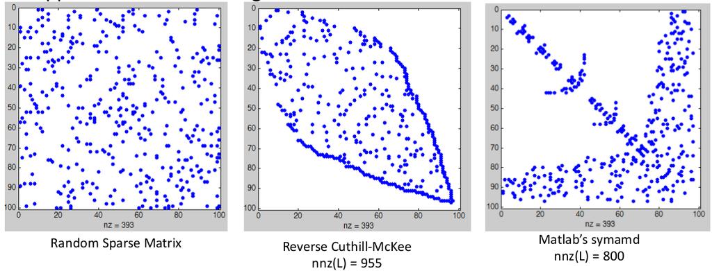
35 Original ordering: 1-A, 2-B, 3-C, 4-D, 5-E, 6-F, 7-G. Minimum degree ordering: 1-A, 2-C, 3-D, 4-E, 5-B, 6-F, 7-G. A P = LU (2.4.23) Remark 16. Minimum degree ordering is a local strategy. No guarantee that it will produce the global minimum fill-ins. Example 22 (Not global minimum fill-ins). Not the end of the story. Matlab s symamd (symmetric approximate minimum degree permutation) can do even better! 53

36 54

37 Yangang Chen, U Waterloo CS 475/675 Notes, Spring 2017 Application: Image denoising (1 lectures) Image denoising Images often contain random noise (small errors), which may result from e.g. the sensors, the capture process, or conditions under which it was captured. Often there is enough signal amidst the noise that we can try to recover a version with the noise removed/reduced. Image denoising: given some observations, reconstruct the source/factors that generated them. 55

38 2.5.2 Mathematical formulation We treat (grayscale) images as 2D scalar functions: u i,j = pixel intensity value at row i, column j Mathematical formulation: given observed image u 0, and true underlying image u, find an approximation of u (u u), in order to eliminate/reduce noise in the solution, or, to minimize the total fluctuation of the pixel values, R(u): min R(u), (2.5.1) u and preserve as much information as possible min u u u = min u u(x) u 0 (x) 2 dx. (2.5.2) 56

39 Image denoising is a trade-off between (2.5.1) and (2.5.2). The optimization problem is given by ( ) min αr(u) + u u (2.5.3) u α is a user-specified parameter. α 0: u u 0. α : u constant. We want something between. So, how do we characterize the total fluctuation of the pixel values, R(u)? Attempt 1: Laplacian regularization Choose R(u) = u 2 2 = u 2 dx. (2.5.4) The optimization (2.5.3) becomes The Euler-Lagrange equation gives us ( ) min α u u u (2.5.5) u α 2 u + u u 0 = 0. (2.5.6) α 2 u + u = u 0. (2.5.7) This is very similar to the 2D Poisson equation. Use finite difference α 4u i,j u i 1,j u i+1,j u i,j 1 u i,j+1 h 2 + u i,j = (u 0 ) i,j. (2.5.8) This gives a linear system: (αa + I)u = u 0. (2.5.9) 57

40 2.5.4 Attempt 2: Total variation regularization Choose L 1 norm instead of L 2 norm: R(u) = u 2 1 = u dx. (2.5.10) The optimization (2.5.3) becomes ( ) min α u u u (2.5.11) u The Euler-Lagrange equation gives us ( ) 1 α u u + u u 0 = 0. (2.5.12) Remark 17 (How does it work?). The coefficients c in characterizes the degree of smoothing! ( ) 1 α u u u + u = u 0. (2.5.13) α (c u) + u = u 0 (2.5.14) depend on gradients in the solution nonlin- For (2.5.13), the coefficients c = 1 ear PDE. u Near edge: u is large, c = 1 is small, small degree of smoothing. u Flat region: u is small, c = 1 is large, large degree of smoothing. u Previous approach is roughly the same, but with the coefficients c = 1. 58

41 We can again apply finite difference and obtain a system of equations (αa(u) + I)u = u 0. (2.5.15) Unlike the previous example, the matrix A depends on u. So it is a nonlinear system of equations. A simple approach to nonlinear equations is fixed point iteration: Freeze the coefficients to make the equations linear, solve, update, and repeat. Algorithm 10 Fixed point iteration for (2.5.15) 1: Pick u (0). 2: for k = 1, 2, until convergence do 3: Solve (αa(u (k 1) ) + I)u (k) = u 0 4: end for Results: 59

42 60