LINEAR SYSTEMS (11) Intensive Computation

Transcription

1 LINEAR SYSTEMS () Intensive Computation 27-8 prof. Annalisa Massini Viviana Arrigoni

2 EXACT METHODS:. GAUSSIAN ELIMINATION. 2. CHOLESKY DECOMPOSITION. ITERATIVE METHODS:. JACOBI. 2. GAUSS-SEIDEL 2

3 CHOLESKY DECOMPOSITION Direct method to solve linear systems, Ax=b. If A is symmetric and positive-definite, it can be written as the product of a lower triangular matrix L and its transpose, A=LL T. L is the Cholesky factor of A. More notions on positive-definite matrices: A matrix is positive-definite iff its eigenvalues are positive iff its principal minors are positive (Silvester s criterion). Eigenvalues: solutions of the characteristic polynomial (spectrum). Principal minors: determinants of the sub matrices on the principal diagonal. 3

4 BRIEF NOTE ON THE GEOMETRIC MEANING OF POSITIVE-DEFINITE MATRICES Since we have already met positive-definite matrices, let s try to visualise them in R 2. x y a c x c b y = ax 2 +2cxy + by 2 >, 8(x, y) 6= (, ) if A is positive-definite, 8(x, y) 6= (, ) if A is positive-semidefinite? if A is indefinite 4

5 POSITIVE-DEFINITE: ELLIPTIC PARABOLOID

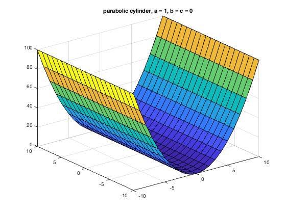
6 POSITIVE-SEMIDEFINITE: PARABOLIC CYLINDER

7 INDEFINITE: HYPERBOLIC PARABOLOID (SADDLE)

8 CHOLESKY DECOMPOSITION step: Given a symmetric square matrix A, we can write it as follows: A2 A22 A2 T a, a,2... a,n a 2, a 2,2... a 2,n a, A B C T 2, A 2, 2 R A A A 2,2 2 R n n 2, A 2,2 a n, a n,2... a n,n Now we want to write A as LL T where L is lower-triangular and can be written as follows: l,... l 2, l 2,2... C. A l n, l n,2... l n,n l, L 2,2 L 2, 8 where L22 is again lower-triangular.

9 CHOLESKY DECOMPOSITION So A=LL T is: a, A T 2, A 2, A 2,2 = l, L 2, L 2,2 l, L T 2, L T 2,2 l 2 =, l, L T 2, l, L 2, L 2, L T 2, + L 2,2 L T 2,2 Remember! We are looking for the entries of L! At this point we can compute the following portions of L: l, = p Basically we get the values a, L 2, = l, A 2, of the entries of the first column of L. Then we compute the following: A 2,2 = L 2, L T 2, + L 2,2 L T 2,2 =) L 2,2 L T 2,2 = A 2,2 L 2, L T 2, =: A (2) 9

10 CHOLESKY DECOMPOSITION 2 step: repeat step on the matrix A (2) =L2,2 L2,2 T. a (2), A (2)T 2, A (2) 2, A (2) 2,2! = A (2) (n ) (n ) 2 R (2),2,A(2) 2,,L (n 2) 3,2 2 R A (2) 2,2,L (n 2) (n 2) 3,3 2 R l2,2 l2,2 L T 3,2 L 3,2 L 3,3 L T 3,3 Iterate until the last sub matrix A (n) is considered. At every step, the size of A (k) decreases of one and the k column of L is computed. l 2,2 = l 2 = 2,2 l 2,2 L T 3,2 l 2,2 L 3,2 L 3,2 L T 3,2 + L 3,3 L T 3,3 q a (2), L 3,2 = l 2,2 A (2) 2, A (2) 2,2 = L 3,2L T 3,2 + L 3,3 L T 3,3 =) L 3,3 L T 3,3 = A (2) 2,2 L 3,2 L T 3,2 =: A (3)

11 CHOLESKY DECOMPOSITION Once we get L, the linear system Ax=b can be written as LL T x=b, so: - Solve Ly=b using forward substitution; - Solve L T x=y using backward substitution. Why does A have to be positive-definite? If A (k) is positive-definite, then: a (k) (it is its first principal minor), hence is well, > defined. is positive-definite. A (k+) = A (k) 2,2 a (k), A 2, A T 2, l k,k = q a (k), 8k =,...,n

12 A AN EXAMPLE A l, l 2, l 2,2 l, l 2, l 3, l 2,2 l 3,2 A = 5 l 3, l 3,2 l 3,3 l 3,3 l, 2 l, l 2, l, l 3, l, l 2, l2, 2 + l2,2 2 l 2, l 3, + l 2,2 l 3,2 A l, l 3, l 2, l 3, + l 2,2 l 3,2 l3, 2 + l3,2 2 + l3,3 2 Thus 5 3 L 2,2 L T 2,2 = A l, = p 25 = 5 L 2, = l2, l 3, = is the first column of L. The matrix for the next iteration is: = = = A (2)

13 AN EXAMPLE step 2 Repeat the same procedure on matrix A (2) : Thus: l 2,2 = p 9=3 So the second column of L is A (3) := = =9 l2,2 l2,2 l 3,2 l 3,2 l 3,3 l 3,3 L 3,2 = l 3,2 = 3 3A =, while: l 2 2,2 l 2,2 l 3,2 l 2,2 l 3,2 l3,2 2 + l3,3 2 3

14 AN EXAMPLE step 3 A (3) =9=L 3,3 L T 3,3 = l 2 3,3 hence: l 3,3 = p 9=3 So the last column of L is In conclusion: A = LL A A 3 3 4

15 AN EXAMPLE Assume b =(,...,) T forward substitution backward substitution Ly = b L T x = b y 2 A A 3 y 3 y 2 A y x 2 A 3 x x 2 A x

16 CHOLESKY DECOMPOSITION Algorithm: Given a linear system Ax=b, A is symmetric and positive-definite and its size is n Initialize L as a nxn zero matrix; For i=:n O(n 3 ) - expensive! L(i,i)= A(i,i); If i < n L(i+:n,i) = A(i+:n,i) / L(i,i); A(i+i:n,i+:n)=A(i+:n,i+:n) - L(i+:n,i) * L(i+:n,i) T ; Solve Ly=b (forward substitution); Solve L T x=y (backward substitution); 6

17 CHOLESKY FOR SPARSE If A is sparse, so may be L. MATRICES If L is sparse, the cost of factorization is less than n 3 /3 and it depends on n, the number of nonzero elements, and the sparsity pattern.. % Fill-in example: a a T I x y = b c Factorization a T a I = a T a L 2,2 L T 2,2 B A = B A B A 7

18 CHOLESKY FOR SPARSE MATRICES This can be solved by shifting columns of A of one position to the left (and swapping entries on vectors x and b), getting no fill-in at all. a a T I Factorization x y = I a a T B A b c = = Shift I a y a T x I p I a T at a 8 C B p a = at a c b C A

19 CHOLESKY FOR SPARSE MATRICES We have seen that permuting the entries of A can prevent fill-in during factorization, so one can factorize a permutation of A instead of A itself. Permutation matrix: square matrix having exactly one on every row and column. If P is a permutation matrix, then PA permutes A s row, AP permutes A s column, P T AP permutes A s rows and columns. Permutation matrices are orthogonal: P T = P -. Instead of factorizing A, one can factorize P T AP in order to prevent fill-in P effects the sparsity pattern of A and it is not known a-priori, but there are heuristic methods to select good permutation matrices. 9

20 FACTS ON CHOLESKY DECOMPOSITION Speaking of methods to avoid pivoting, as the transpose and the exponential methods produce positive-definite matrices, the Cholesky decomposition may be applied. Gaussian elimination vs. Cholesky decomposition: The Gaussian elimination can be applied to any matrix, even to non square ones, while the Cholesky decomposition can be applied only on (square) symmetric and positive-definite matrices. They have the same asymptotic computational cost (O(n 3 )), but Cholesky is faster by a factor 2. 2

21 EXACT METHODS:. GAUSSIAN ELIMINATION. 2. CHOLESKY DECOMPOSITION. ITERATIVE METHODS:. JACOBI. 2. GAUSS-SEIDEL

22 ITERATIVE METHODS Iterative methods for solving a linear system Ax=b consist in finding a series of approximate solutions x, x 2, etc., starting from an initial approximate solution x until convergence to the exact solution. Iteration can be interrupted when the desired precision is reached. For example: precision threshold, ε = -3. Suppose the error is computed as the absolute value of the difference of the exact and the approximate solutions element- wise, xi - x k i. It follows that an approximate solution x k is accepted if xi - x k i < ε. Assume the solution of Ax=b is x=(,,) T, the approximate solution x k =(.9,,.9) T satisfies the threshold. 22

23 ITERATIVE METHODS Iterative methods are usually faster than exact methods, specially if the coefficient matrix is large and sparse. One can play with the threshold to find the desired tradeoff between speed and accuracy (increasing the precision threshold reduces the number of iterations to reach acceptable approximate solutions, but at the same time it produces less accurate solutions). On the other hand, for some problems convergence may be very slow or the solution may not converge at all. 23

24 EXACT METHODS:. GAUSSIAN ELIMINATION. 2. CHOLESKY DECOMPOSITION. ITERATIVE METHODS:. JACOBI. 2. GAUSS-SEIDEL 24

25 JACOBI METHOD Strictly diagonally dominant matrix: The absolute value of the diagonal entries is strictly greater than the sum of the absolute value of the non diagonal entries of the corresponding rows. a i,i > n P j= j6=i a i,j 8i =...n The Jacobi method always succeeds if A or A T are strictly diagonally dominant. * if the system is not strictly diagonally dominant, it may still converge. We will consider strictly diagonally dominant linear systems. 25

26 JACOBI METHOD Given the linear system: a, x + a,2 x a,n x n = b a 2, x + a 2,2 x a 2,n x n = b 2. a n, x + a n,2 x a n,n x n = b n where A is strictly diagonally-dominant, it can be rewritten as follows by isolating xi in the i equation: x = b a,2 a, a, x 2... x 2 = b 2 a 2, a 2,2 a 2,2 x... a,n a, x n a 2,n a 2,2 x n. x n = b n a n,n a n, a n,n x a n,2 a n,n x

27 JACOBI METHOD Let x () =(x (),...,x() n ) x () is the zero vector). be the initial approximate solution (commonly Find the approximate solution x () by substituting x () in the right hand side of the linear system: x () = b a, a,2 a, x () 2... x () 2 = b 2 a 2,2 a 2, a 2,2 x ()... a,n a, x () n a 2,n a 2,2 x () n. x () n = b n a n, a n,n a n,n x () a n,2 a n,n x () 2... Then use the approximate solution x () just computed to find x (2) by substituting x () in the right hand side of the linear system. 27

28 JACOBI METHOD Iterate. At the k step one finds the approximate solution x (k) by substituting the previous one in the right hand side of the linear system: x (k) = b a, a,2 x (k) 2 = b 2 a 2,2 a 2, (k ) a, x (k ) a 2,2 x a,n (k ) a, x n a 2,n (k ) a 2,2 x n. x (k) n = b n a n,n a n, (k ) a n,n x a n,2 (k ) a n,n x 2... If A is strictly diagonally-dominant, the produced approximate solutions are more and more accurate. 28

29 JACOBI - STOPPING CRITERIA When should one stop iterating? When the error produced is small enough. Different ways to compute the error at each step: e (k) := x (k+) -x (k) : the error is the difference between the last and the previous solutions. e (k) := x-x (k) : the error is the difference between the exact solution and the approximate solution(exact solution is usually unknown tho). e (k) := x (k+) -x (k) / x (k+) : the error is the change rate between the last and the previous solutions. where. is the l 2 norm: x 2= (x 2 + +xn 2 ). So the iterations are repeated while e (k) >= ε 29

30 AN EXAMPLE The linear system 9x + y + z = 2x + y +3z = 9 3x +4y + z = has x y z A 2 A Since A is strictly diagonally dominant, the system can be solved with Jacobi. Compute the error as e (k) := x (k+) -x (k) and let x () =(,,) be the initial approximate solution. x () = 9 ( y() z () )= 9 y () = (9 2x() 3z () )= 9 z () = ( 3x() 4y () )= So the first approximate solution is x (): (x, y, z) T =( 9, 9, )T The error is: e () =2.2. 3

31 AN EXAMPLE Substituting x () we get: x (2) = 9 ( y() z () )= 9 ( 9 )= 9 y (2) = (9 2x() 3z () )= (9 2 9 z (2) = ( 3x() 4y () )= ( and the error is: e () =.4. One more iteration: x (3) = 9 ( y(2) z (2) )= 9 ( )= 5 9 )= )=.353 y (3) = (9 2x(2) 3z (2) )= ( z (3) = ( 3x(2) 4y (2) )= ( )= 8 9 The error is: e (2) =.395 )=

32 AN EXAMPLE Assume the required precision is ε = -3. Then after iteration the error is x -4. and the approximate solution is x y () A = z 2. A

33 JACOBI METHOD Algorithm: Given Ax=b, where A is strictly diagonally dominant: Initialize the first approximate solution x and an array x and set err=inf and ε; while err >= ε for i = :n x(i) = b(i); for j = :n if j!= i x(i) = x(i) - A(i,j) * x(j); x(i) = x(i) / A(i,i); update err; x = x; 33 O(#of iterations x n 2 )

34 JACOBI METHOD If k is the number of iterations (in the while), then the number of operations executed by the Jacobi algorithm is kn 2. The Gaussian elimination requires n 3 /3 operations. So it is more convenient to use the Jacobi method instead of the Gaussian elimination if kn 2 < n 3 /3, that is when k<n/3. For this reason it is important to assess the minimum number of iterations before deciding whether to apply Jacobi. Such number is the smallest k that satisfies: k> log( ( ) ) log( ) where 34 = max i=,...,n np j= j6=i a i,j a i,i = max i=,...,n x() i x () i

35 JACOBI - MATRICIAL FORM Given Ax=b, where A is strictly diagonally dominant, one can write A as follows: a, a,2... a,n a,... a 2, a 2,2... a 2,n B A = a 2,2... C. A a n, a n,2... a n,n... a n,n 2... a 2,... 6B 4@.... C.. A a n, a n, a,2... a,n... a 2,n C7. A5... A = D [ L U ] So the linear system can be rewritten as: {D [ L U]}x = b If A is diagonally dominant, D is invertible, so: Dx [ L U]x = b $ x D [ L U]x = D b $ x = D [ L U]x + D b Matricial form of Jacobi: x (k+) = D [ L U]x (k) + D b 35 k =,, 2,...

36 EXACT METHODS:. GAUSSIAN ELIMINATION. 2. CHOLESKY DECOMPOSITION. ITERATIVE METHODS:. JACOBI. 2. GAUSS-SEIDEL

37 GAUSS-SEIDEL Iterative method, very similar to Jacobi s. It always converges if A is strictly diagonally dominant or symmetric and positive-definite. x (k) = b a,2 (k ) x 2 a, a, x (k) 2 = b 2 a 2, x (k) a 2,2 a 2,2 a 2,3 a,3 (k ) x 3... a, (k ) x 3... a 2,2 a 2,n a,n a, x a 2,2 x (k ) n (k ) n x (k) 3 = b 3 a 3, x (k) a 3,3 a 3,3. x (k) n = b n a n, x (k) a n,n a n,n a 3,2 a 3,3 x (k) 2... a n,2 a n,n x (k) a 3,n a 3,3 x a n,n a n,n (k ) n x (k) n * if the system is not strictly diagonally dominant nor positive-definite, it may still converge. We will consider strictly diagonally dominant or positive-definite linear systems.

38 AN EXAMPLE The same linear system we used before: 9x + y + z = 2x + y +3z = 9 3x +4y + z = Compute the error as e (k) := x (k+) -x (k) and let x () =(,,) be the initial approximate solution. x () = 9 y () z () = 9 y () = x() z() = = 5 9 z () = 3 x() 4 y() = = error =

39 AN EXAMPLE Second iteration: x (2) = 9 9 y() 9 z() = = y (2) = x(2) z() = = z (2) = 3 x(2) 4 y(2) = = error =

40 AN EXAMPLE If the error threshold is -3, after 5 iterations we get: ya = 2 A Computed error: * -4 In iteration 4, the approximate solution was: ya = 2 A Computed error:.34. 4

41 GAUSS-SEIDEL-MATRICIAL FORM Write A as follows: a, a,2... a,n a 2, a 2,2... a 2,n B A = a n, a n,2... a n,n a,... a 2,2... C. A... a n,n 2... a 2,... 6B 4@.... C.. A a n, a n, a,2... a,n... a 2,n C7. A5... A = D [ L U ] Then the linear system can be written as: (D + L + U)x = b Then: (D + L)x + Ux = b So the matricial form of Gauss-Seidel is: (D + L)x (k+) = b Ux (k) 8k =,, 2,... 4

42 GAUSS-SEIDEL Algorithm: Given Ax=b, where A is strictly diagonally dominant or positive-definite: Initialize x, x arrays of length n. Set err=inf and ε; while err ε for i = :n x(i) = x(i) \ A(i,i); x(i) = b(i); Update err; if i == x = x; for j = 2:n x(i) = x(i) - A(i,j) * x(j); else for j = :i - x(i)=x(i) - A(i,j) * x(j); O(#of iterations x n 2 ) for j = i + :n x(i) = x(i) - A(i,j) * x(j); 42

43 JACOBI VS. GAUSS-SEIDEL On several classes of matrices, Gauss-Seidel converges twice as fast as Jacobi (meaning that at every iteration, the number of fixed exact solution digits that Gauss-Seidel computes is twice as large as Jacobi s). As soon as the improved entries of the approximate solution are computed, they are immediately used in the same iteration step, k. On the other hand, Jacobi can be parallelized, while Gauss-Seidel is inherently non parallelizable. The same stopping criteria work for both methods. 43