Turbulent Characteristics in Stirring Vessels: A Numerical Investigation

Transcription

1 Turbulent Characteristics in Stirring Vessels: A Numerical Investigation By Vasileios N. Vlachakis Thesis submitted to the faculty of the Virginia Polytechnic Institute and State University in partial fulfillment of the requirements for the degree of Master of Science In Mechanical Engineering APPROVED: Pavlos P. Vlachos, Committee Chair Demetri P. Telionis, Committee Member Roe-Hoan Yoon, Committee Member Danesh Tafti, Committee Member June 16, 2006 Blacksburg, Virginia Keywords: Rushton turbine, Stirring Vessel, Turbulence, CFD, FLUENT, DPIV Copyright 2006, Vasileios N. Vlachakis

2 ABSTRACT TURBULENCE CHARACTERISTICS IN STIRRING VESSELS: A NUMERICAL INVESTIGATION Vasileios N. Vlachakis Understanding the flow in stirred vessels can be useful for a wide number of industrial applications, like in mining, chemical and pharmaceutical processes. Remodeling and redesigning these processes may have a significant impact on the overall design characteristics, affecting directly product quality and maintenance costs. In most cases, the flow around the rotating impeller blades interacting with stationary baffles can cause rapid changes of the flow characteristics, which lead to high levels of turbulence and higher shear rates. The flow is anisotropic and inhomogeneous over the entire volume. A better understanding and a detailed documentation of the turbulent flow field is needed in order to design stirred tanks that can meet the required operation conditions. This thesis describes efforts for accurate estimation of the velocity distribution and the turbulent characteristics (vorticity, turbulent kinetic energy, dissipation rate) in a cylindrical vessel agitated by a Rushton turbine (a disk with six flat blades) and in a tank typical of flotation cells. Results from simulations using FLUENT (a commercial CFD package) are compared with Time Resolved Digital Particle Image Velocimetry (DPIV) for baseline configurations in order to validate and verify the fidelity of the computations. Different turbulence models are used in this study in order to determine the most appropriate for the prediction of turbulent properties. Subsequently, a parametric analysis of the flow characteristics as a function of the clearance height of the impeller from the vessel floor is performed for the Rushton tank as well as the flotation cell. Results are presented for both configurations along planes normal or parallel to the impeller axis, displaying velocity vector fields and contour plots of vorticity, turbulent dissipation and others. Special attention is focused in the neighborhood of the impeller region and the radial jet generated there. The flow in this neighborhood involves even larger gradients and dissipation levels in tanks equipped with stators. The present results present useful information for the design of the stirring tanks and flotation cells, and provide some guidance on the use of the present tool in generating numerical solutions for such complex flow fields. Keywords: Stirring tank; Turbulence; DPIV; FLUENT; Rushton turbine;

3 ACKNOWLEDGMENTS The completion of this thesis would not have been possible without the help of many individuals. First I would like to thank my advisor, Dr. Pavlos Vlachos, for helping me in my first difficult steps in the US and for giving me the opportunity to work on this project. His patience and comments helped me to make this work better. I would also like to thank Professor Telionis for providing me with useful directions and discussions in my quest for solutions as well as for showing the scientific path in order to enrich my knowledge. I will always be grateful to Professor Yoon for having me involved to his flotation group from which I gained a lot. Last but not least I am thankful to Professor Tafti for having his door open every time a question arose. The collaboration with him helped me develop my computational thought and intuition. I will never forget the guys in my office and in the fluids lab who helped me a lot and kept me company all this time. A big thank you goes to Mike Brady who was as a second advisor in my way to explore the world of the experiments and to Yihong Yang who helped me greatly in the last months of my effort. I will never forget all my Greek, Cypriot and International friends that I made here at Virginia Tech when I started my graduate studies. You gave me freely your company and I am honored to be your friend. I also am thankful to my friends in Greece who did not forget about me when I decided to continue my studies on the other side of the world. Finally, I am grateful to my parents for believing in me in all the steps of my life. My gratitude is the least reward for their contribution. Thanks for your love and for being there to support me in everything, even from so far away. Above all, I would like to thank God for getting me to the position I am today and being the source of my internal strength. "If we knew what it was we were doing, it would not be called research, would it?" Albert Einstein Dedicated to the memory of my grandmother Elisavet Vlachaki

4 TABLE OF CONTENTS INTRODUCTION...X CHAPTER STIRRING TANK MODEL GOVERNING EQUATIONS STIRRING TANK SIMULATIONS RESULTS-DISCUSSION CONCLUSIONS...9 CHAPTER INTRODUCTION THE FLOTATION PROCESS CONFIGURATION AND PARTS OF THE DORR-OLIVER FLOTATION CELL RESULTS...28 APPENDIX I...64 RUSHTON TURBINE...64 A. OUTLINE OF TURBULENCE MODELS FOR THE STIRRING TANK SIMULATIONS...64 B. GRID STUDY...69 C. CFD SIMULATIONS OF A RUSHTON TANK AND A FLOTATION CELL...71 D. THE MULTI-REFERENCE SYSTEM...72 E. NON DIMENSIONAL NUMBERS...74 F. MORE RESULTS CONCERNING THE RUSHTON TURBINE...78

5 NOMENCLATURE Symbol Explanation Dimensions D or D T Tank Diameter m ves D or D imp Impeller Diameter m I T or H Tank Height m ves H Impeller Height m imp N Impeller Rotational Speed 1/sec C Clearance: Distance of the impeller from the bottom of the Tank m g Acceleration due to gravity 2 m /sec ρ Liquid Density kg/m 3 σ Parameters in k-ε model - c Parameters in k-ε models - r Radial distance from m center of impeller z vertical direction from m center of impeller ν Kinematic Viscosity m 2 /sec v turb Turbulent eddy viscosity m 2 /sec ν Effective eddy viscosity m 2 /sec eff Re Reynolds Number - u tip Impeller tip speed m/sec ' u Fluctuation from the i- m/sec i velocity component u i Liquid Velocity in i- Direction m/sec uu Components of the m 2 /sec i j Reynolds stresses w Baffles width m bf w bl Impeller Blade Width m th Impeller Blade thickness m bl th Baffle thickness m bf τ d Dissipation rate time scale sec η Kolmogorov length scale m ε Dissipation rate 2 3 1/ m sec ii

6 k Turbulent kinetic energy 2 2 m /sec S Strain rate Tensor m 2 /sec ij P Production of turbulent k kinetic energy p Pressure Pa Wm 3 iii

7 ACRONYMS Abbreviations CFD 2D 3D DPIV LES DNS RSM RANS MRF SM Explanation Computational Fluid Dynamics Two-dimensional Three dimensional Digital Particle Image Velocimetry Large Eddy Simulations Direct Numerical Simulations Reynolds Stress Model Reynolds Averaged Navier-Stokes Multi Reference Frame Sliding Mesh iv

8 LIST OF FIGURES Figure 1.1: Rushton Tank and Impeller Configuration...4 Figure 1.2: Normalized radial velocity at the centerline of the impeller Figure 1.3: Normalized radial velocity using the Standard k-ε model for Re=35000 at r/ D T = 0 for C/ T = 1/15 (top frame), for C/ T = 1/2 (middle frame) and for C/ T = 1/3 (bottom frame)...13 Figure 1.4: Normalized Dissipation using the Standard k-ε model rate for Re=35000 at r/ D T = 0 for C/ T = 1/15 (top frame), for C/ T = 1/2 (middle frame) and for C/ T = 1/3 (bottom frame) Figure 1.5: Normalized Dissipation rate at the centerline of the impeller...15 Figure 1.6: Normalized maximum dissipation rate versus the Re number for C/ T = 1/15 (top frame), for C/ T = 1/2 (middle frame) and for C/ T = 1/3 (bottom frame) Figure 1.7: Normalized Turbulent Kinetic Energy using the Standard k-ε model for Re=35000 at z/ D T = 0 for C/ T = 1/15 (top frame), for C/ T = 1/2(middle frame) and for C/ T = 1/3(bottom frame) Figure 1.8: Normalized TKE at the centerline of the impeller with and without periodicity for Re= Figure 1.9: Normalized Z vorticity using the Standard k-ε model for Re=35000 at z/ D T = 0 for C/ T = 1/15(top frame), for C/ T = 1/2(middle frame) and for C/ T = 1/3 (bottom frame)...20 Figure 1.10: Normalized Xvorticity using the Standard k-ε model for Re=35000 at r/ D T = 0 for C/ T = 1/15(top frame), for C/ T = 1/2(middle frame) and for C/ T = 1/3 (bottom frame)...21 Figure 1.11: Normalized radial velocity profiles at r/t=0.256 (top frame) and at r/t=0.315 (bottom frame) for C/ T = 1/2 and Re= Figure 1.12: Normalized Dissipation rate profiles at r/t=0.256 (top frame) and at r/t=0.315 (bottom frame) for C/ T = 1/2 and Re= Figure 2.1: Configuration of the Dorr-Oliver Stirring Tank...27 Figure 2.2: Dorr-Oliver Impeller...27 Figure 2.3: Dorr-Oliver Stator...28 Figure 2.4: Contour Plots of the normalized velocity magnitude using the Standard k-ε model for the three configurations...30 Figure 2.5: Contour Plots of the radial velocity using the Standard k-ε model for the three configurations (impeller blade plane)...32 Figure 2.6: Contour Plots of the normalized TKE using the Standard k-ε model for the three configurations...34 Figure 2.7: Contour Plots of the normalized Dissipation rate using the Standard k-ε model for the three configurations...36 Figure 2.8: Contour Plots of the normalized Z-vorticity using the Standard k-ε model for the three configurations...37 v

9 Figure 2.9: Contour Plots of the normalized Z-vorticity using the Standard k-ε model for the three configurations in a plane between the rotor blades ( x/ Dves = 0)...39 Figure 2.10: Streamlines using the Standard k-ε model for all three configurations in a horizontal slice that passes through the first one forth of the impeller ( y/ H imp = 1/4)...41 Figure 2.11: Streamlines using the Standard k-ε model for all three configurations in a horizontal slice that passes through the middle of the impeller ( y/ H imp = 1/ 2 )...43 Figure 2.12: Streamlines using the Standard k-ε model for all three configurations in a horizontal slice that passes through the last one forth of the impeller ( y/ H imp = 3/ 4 )...44 Figure 2.13: Normalized Y-vorticity using the Standard k-ε model for all three configurations in a horizontal slice that passes through the first one forth of the impeller ( y/ H imp = 1/4)...47 Figure 2.14: Normalized Y-vorticity using the Standard k-ε model for all three configurations in a horizontal slice that passes through the first one forth of the impeller ( y/ H imp = 1/ 2 )...48 Figure 2.15: Normalized Y-vorticity using the Standard k-ε model for all three configurations in a horizontal slice that passes through the first one forth of the impeller ( y/ H imp = 3/ 4 )...50 Figure 2.16: Normalized TKE using the Standard k-ε model for all three configurations in a horizontal slice that passes through the first one forth of the impeller ( y/ H imp = 1/4)...52 Figure 2.17: Normalized TKE using the Standard k-ε model for all three configurations in a horizontal slice that passes through the first one forth of the impeller ( y/ H imp = 1/ 2 )...53 Figure 2.18: Normalized TKE using the Standard k-ε model for all three configurations in a horizontal slice that passes through the first one forth of the impeller ( y/ H imp = 3/ 4 )...55 Figure 2.19: Normalized Dissipation rate using the Standard k-ε model for all three configurations in a horizontal slice that passes through the first one forth of the impeller ( y/ H imp = 1/4)...57 Figure 2.20: Normalized Dissipation rate using the Standard k-ε model for all three configurations in a horizontal slice that passes through the first one forth of the impeller ( y/ H imp = 1/ 2 )...58 Figure 2.21: Normalized Dissipation rate using the Standard k-ε model for all three configurations in a horizontal slice that passes through the first one forth of the impeller ( y/ H imp = 3/ 4 )...60 Figure 2.22: Normalized Y-isovorticity using the Standard k-ε model for all three configurations...61 Figure I.1: Normalized radial velocity at the centerline of the impeller for all the grids and turbulence models...70 vi

10 Figure I.2: Normalized TKE at the centerline of the impeller for all the grids and turbulence models...70 Figure I.3: Normalized dissipation rate at the centerline of the impeller for all the grids and turbulence models...71 Figure I.4: Stirring Tank configuration: (a) Three dimensional and (b) Cross sectional view of the tank...72 Figure I.5: Computational Grid for simulations with the MRF model...73 Figure I.6: Power Number versus Re number...77 Figure I.7: Effect of the baffles and impeller size on the Po number...77 Figure I.8: Normalized radial velocity (top frame) and velocity magnitude (bottom frame) at the centerline of the impeller for all the three different configurations for Re= Figure I.9: Normalized dissipation rate (top frame) and turbulent kinetic energy (bottom frame) at the centerline of the impeller for all the three different configurations for Re= Figure I.10: Normalized X-vorticity (top frame) and tangential velocity (bottom frame) at the centerline of the impeller for all the three different configurations for Re= Figure I.11: Normalized radial velocity (top frame) and velocity magnitude (bottom frame) at the centerline of the impeller for all the three different configurations for Re= Figure I.12: Normalized dissipation rate (top frame) and turbulent kinetic energy (bottom frame) at the centerline of the impeller for all the three different configurations for Re= Figure I.13: Normalized X-vorticity (top frame) and tangential velocity (bottom frame) at the centerline of the impeller for all the three different configurations for Re= Figure I.14: Normalized velocity magnitude (top frame) and tangential velocity (bottom frame) at the centerline of the impeller for all the three different configurations for Re= Figure I.15: Normalized X-vorticity at the centerline of the impeller for all the three different configurations for Re= Figure I.16: Streamlines at z/ DT = ± 0.2(above and below the impeller)...89 Figure I.17: Contour Plots of the Normalized Y-vorticity using the Standard k-ε model at a plane that passes through the end of the blades for C/ T = 1/2 and Re= D view (top frame) and details (bottom frame)...90 Figure I.18: Normalized radial velocity (top frame) and dissipation rate profiles (bottom frame) at r/t=0.19 for C/ T = 1/2and Re=35000 with all the tested turbulence models...92 Figure I.19: Normalized radial velocity (top frame) and dissipation rate profiles (bottom frame) at r/t=0.256 for C/ T = 1/2 and Re=35000 with all the tested turbulence Models...93 Figure I.20: Normalized radial velocity (top frame) and dissipation rate profiles (bottom frame) at r/t=0.256 for C/ T = 1/2 and Re=35000 with all the tested turbulence models...94 Figure I.21: Normalized radial velocity (top frame) and X-vorticity (bottom frame) at the centerline of the impeller for C/ T = 1/2and Re= vii

11 Figure I.22: Normalized dissipation rate (top frame) and turbulent kinetic energy (bottom frame) at the centerline of the impeller for C/ T = 1/2 and Re= Figure I.23: Normalized Reynolds stresses ( uu r z component) at the centerline of the impeller for C/ T = 1/3 and Re= Figure I.24: Normalized Z-Isovorticity using the Standard k-ε model, 3D View (left frame) and Zoom in view (right frame)...98 viii

12 LIST OF TABLES Table 1.1: Simulation Test Matrix...7 Table 2.1: Simulation Matrix for the Dorr-Oliver Tank...26 Table I.1: Parameters for the Standard k-ε model...65 Table I.2: Parameters for the RNG k-ε model...66 Table I.3: Parameters for the Realizable k-ε model...68 ix

13 INTRODUCTION This thesis represents part of the work of a team of researchers from mining engineering, mechanical engineering and engineering mechanics on flotation processes. The present work is computational modeling of stirring tanks and flotation cells, using a CFD code (Computational Fluid Dynamics) by Fluent. The thesis is prepared in a format recently approved by the Dean of the VA Tech Graduate School. The material is presented in very concise manner, in the form of a journal publication. The idea is that, a paper can be submitted for publication without any further modifications. Results that were not included in the main body of the thesis due to lack of space can be found in the Appendix. In the first chapter we explore the flow in a typical stirring tank. This is a cylindrical container equipped with an agitating impeller. This is a classical problem that has been extensively investigated before. The aim of the present work is essentially to use this case as a benchmark, in order to validate the computational method. The results are compared with earlier numerical and experimental data, as well as the experimental results obtained by members of the VA Tech team. The present work was extended to consider two configurations not yet explored by other investigators. This is the effect on the hydrodynamics of placing the impeller closer to the bottom of the tank. This configuration is closer to the needs of flotation technology and the mining industry. Another issue that was explored with greater detail than earlier reported is the effect of the Reynolds number. In the second chapter we examine a different configuration, typical of a flotation cell. This chapter is designed so that it can be presented as another independent paper. As a result there is some repetition of the fundamental material found in the first chapter. Actually this chapter includes a larger number of results, because it will also serve as a final report to the sponsor. It will therefore require some shortening before submission to an archival journal. x

14 CHAPTER Background and Introduction In many industrial and biotechnological processes, stirring is achieved by rotating an impeller in a vessel containing a fluid (stirred tank). The vessel is usually a cylindrical tank equipped with an axial or radial impeller. In most cases, baffles are mounted on the tank wall along the periphery. Their purpose is to prevent the flow from performing a solid body rotation (destroy the circular flow pattern) [1], to inhibit the free surface vortex formation which is present in unbaffled tanks [2] and to improve mixing. However, their presence makes the simulations more difficult and demanding as they remain stationary while the impeller rotates. There are two types of stirring, laminar and turbulent. Although laminar stirring has its difficulties and has been studied in the past [1] by many authors, in most industrial applications where large scale stirring vessels are used, turbulence is predominant. Turbulent flows are far more complicated and a challenging task to predict due to their chaotic nature [4], [5]. In the case of stirred tanks, not only is the flow fully turbulent, but it is also strongly inhomogeneous and anisotropic due to the energetic agitation induced by the impeller. In addition, the flow is periodic, because of the interaction between the blades and the baffles. This leads to periodic velocity fluctuations, which are often referred to as pseudo-turbulence [6]. Energy is transported from the large to the small eddies and then dissipated into the smallest ones according to the Kolmogorov s energy cascade. The size of these smallest eddies can be calculated from the following equation: 3 4 η = Re (1.1) D I However in stirring tanks we have additional energy coming from the rotation of the impeller that is smaller than the energy from the large eddies but larger than that is dissipated into the smallest scales. Thus this energy is located in the middle of the energy spectrum [7]. There are many parameters such as the type and size of the impeller, its location in the tank (clearance), and the presence of baffles that affect the nature of the generated flow field. All these geometrical parameters and many others (e.g. rotational speed of the impeller) make the optimum design of a stirring tank a difficult and time consuming task. [8] 1

15 Accurate estimation of the dissipation rate ( ε ) distribution and its maximum value in stirred tanks, especially in the vicinity of the impeller is of great importance. This is because of a plethora of industrial processes such as particle, bubble breakup, coalescence of drops in liquid-liquid dispersions and agglomeration in crystallizers require calculation of the eddy sizes which are related directly to the turbulent kinetic energy and the dissipation rate [1], [9], [10] In the last two decades significant experimental work has been published contributing to the better understanding of the flow field and shedding light on the complex phenomena that are present in stirred tanks. In most of these studies accurate estimation of the turbulent characteristics and the dissipation rate were the other important aspects [2], [4], [8] There is a wealth of numerical simulations of stirring vessels. In most of these studies the Rushton turbine [10], [11], [12], [13], [14], [15] was used while in others, the pitched blade impeller (the blades have an angle of 45 degrees) [9] or combination of the above two [8], [15] was considered. Only a few of these were carried out using Large Eddy Simulations (LES) in unbaffled [2] and baffled stirred tanks [1], [5], [16]. A variety of different elevations of the impellers and Reynolds numbers were considered. Today, continuing increase of computer power, advances in numerical algorithms and development of commercial Computational Fluid Dynamics (CFD) packages create a great potential for more accurate and efficient three dimensional simulations. In this study we employ a CFD code to analyze the flow in a baffled tank agitated by a Rushton impeller. The selection of the impeller and the stirring tank geometrical parameters were made to facilitate comparisons with available experimental data. The primary objective of this study is to produce numerically a complete parametric study of the time-averaged results based on the Reynolds number, the turbulence models and the clearance of the impeller. The CFD results are compared with those obtained by the present team via a Digital Particle Image Velocimetry. These data were generated with sufficient temporal resolution capable to resolve the global evolution of the flow. The commercial package FLUENT [17] was used for the simulation and the package GAMBIT [18] as a grid generator. MIXSIM [19] is another commercial package specialized in stirring having a library with a variety of industrial impellers. 2

16 A number of different turbulence models are available in FLUENT as in most of the CFD commercial packages. The choice of an appropriate turbulence model is of great significance for getting an accurate solution. In this work we used mostly the k-ε two-equation models. These models have been extensively tested in many applications. The k-ε models are based on the assumption of homogenous isotropic turbulent viscosity, which is not strictly consistent with our case. And yet they predict quite well the velocity distribution and the dissipation rate. We also used the RSM model. Although this model is more general than the two-equation models, it is computationally time consuming because it consists of seven equations for the turbulence modeling, allowing the development of anisotropy, or reorientation of the eddies in the flow. It should therefore provide good accuracy in predicting flows with swirl, rotation and high strain rates Stirring Tank Model Three dimensional simulations were carried out in a baffled cylindrical vessel with diameter D = m(Figure 1a). Four equally spaced baffles with width w = 0.1D and T thickness th = D /40 were mounted on the tank wall. The tank was agitated by a Rushton bf I turbine (disk with six perpendicular blades) with diameter D = D / 3, disk diameter D = 0.75D, blade width w = D / 4, blade height h = 0.2D blade D I bl thicknessth = 0.01D. (Figure 1b, 1c) The working fluid was water and its height was equal to bl I the height of the tank. This model is identical to the model employed in the experimental work carried out by the present team. I bl I bf T I T 3

17 b. a. c. Figure 1.1: Rushton Tank and Impeller Configuration 1.3. Governing Equations The continuity equation and the momentum equations for three dimensional incompressible unsteady flows are given as follows [20], [21], [22]: ρ + = t ( ρu) 0 u 2 ρ + ( uu) = p + 2µ S µ ( u) + F t 3 where S is the rate of the stress tensor and is given by: (1.2) (1.3) S = 2 Sij Sij (1.4) S ij 1 u u i j = + 2 x j x i (1.5) 4

18 Although body forces include gravitational, buoyancy, porous media and other user defined forces in our case includes only the gravitational force. In the case of the steady state simulations the first term on the left hand side in both the continuity and the momentum equation is zero. Velocity (u) and pressure (p) can be decomposed into the sum of their mean ( u, fluctuation components ( u ', p ' ): ' ' u u u and p p p p) and the = + = + (1.6) Noting the rules for averaging: u u u ' = and = 0 (1.7) The above two rules state that the average of the average velocity is equal again to the average and that the average of the fluctuating component is equal to zero. By applying (1.6) and (1.6) into (1.1) and (1.2) in which already we had got rid of the first terms we obtain the time averaged governing equations: u = 0 (1.8) 2 ' ' ρ ( uu) = p + 2µ S µ ( u) + ρg ρ ( u u ) (1.9) 3 The last term is the divergence of the Reynolds stress tensor. It comes from the convective derivative. So strictly, the Reynolds stresses are not stresses; they are the averaged effect of turbulence convection. Modeling is usually achieved using the Boussinesq s hypothesis. In this case the turbulent viscosity depends only the turbulent structure and not on the fluid properties [16]. uu u u i j δ ν = + 3 x j x i ' ' 2 i j k ij t (1.10) 1.4. Stirring Tank Simulations Three-dimensional simulations were carried out in three sets of calculations, using three different clearance heights of the impeller. In the first the clearance was set to 5

19 C/ D T = 1/2(impeller in the middle of the tank) and five Reynolds numbers (Re) in the range to were chosen. The Reynolds number was based on the impeller diameter, Re=ND 2 I /ν. For every Re number three turbulence models, namely Standard k ε, RNG k ε and Reynolds Stress model were tested in order to investigate their predictive accuracy in this kind of flow. In the second set of calculations the clearance of the impeller was set to C/ D T = 1/15(impeller almost at the bottom of the tank) and simulations were performed again but this time using only one of the above three turbulence models that had the best overall performance. In the last configuration the proximity to the ground was set to C/T=1/3 and two turbulence models were tested, the standard k-ε and the Reynolds Stress model. The latter had been chosen due to the availability of experimental data from the literature about the Reynolds stresses. More information about the test cases is listed in Table 1.1. In all sets of calculations, the origin of the coordinate system was fixed in the center of the impeller. The domain of integration was meshed with the aid of the commercial grid generator package GAMBIT creating a hybrid three dimensional grid. The hybrid grid is actually an unstructured grid that contains different types of elements. In our study quadrilaterals and triangle elements were used to construct the mesh. The choice of having an unstructured grid versus a structured one was made due to the fact that in a complex flow like the present, details of the flow field everywhere in the tank and especially in the discharge area of the impeller and behind the baffles must be captured. Then the model was launched to FLUENT for the simulation part. Although FLUENT does not use a cylindrical coordinate system, all the notation in this study was converted to cylindrical making the following changes in notation: x= r, y= ϕ and z z The simulations were accomplished using the steady-state Multi Reference Frame (MRF) approach that is available in FLUENT. In this approach the grid is divided in two or more reference frames to account for the stationary and the rotating parts. In the present case the mesh consists of two frames, one for the tank away from the impeller and one including the impeller. The latter rotates with the rotational speed of the impeller but the impeller itself remains stationary. The unsteady continuity and the momentum equations are solved inside the rotating frame while in the outside stationary frame the same equations are solved in a steady 6

20 form. At the interface between the two frames a steady transfer of information is made by FLUENT. One drawback of the MRF approach is that the interaction between the impeller and the baffles is weak. Table 1.1: Simulation Test Matrix 3 10 Re Standard k-e 1a 2a 3a 4a 5a C/ D T = 1/2 RNG k-e 1b 2b 3b 4b 5b Reynolds 1c 2c 3c 4c 5c Stresses 3 10 Re C/ D T = 1/15 Standard k-e C/ D T = 1/3 Standard k-e Results-Discussion Figure 1.2 shows the distribution of the radial velocity across the centerline of the impeller for all the turbulence models and configurations tested. We observe that all the models predict the radial velocity quite well. This plot can also verify the low speed radial jet produced by the impeller for low clearance configuration (C/T=1/15). Figure 1.3 shows the contour plots of the spatial distribution of the radial velocity superimposed with streamlines in the baffle plane ( r/ D T = 0) for the three configurations. In the case of the low clearance, only one large recirculation area on each side of the tank is observed, while in the other cases, two distinct toroidal zones above and below the impeller divide the flow field in two parts (in half for the case of C/T=1/2 and in one third in the case of C/T=1/3). According to [1] these large-scale ring vortices [21] act as a barrier to stirring by increasing the blend time. It can also be noticed that in the latter cases the radial jet is more energetic than it is in the first. Figure 1.4 presents the contours of the dissipation rate in the impeller e plane ( r/ D T = 0) for all the tested configurations. The maximum dissipation was calculated in a rectangular region along the tip of the blade. Although in this study we present the maximum dissipation 7

21 found in this box, the result is very sensitive to its definition, especially as we go closer to the blade, because the value of the maximum dissipation changes drastically. Despite the fact that the RNG k-e model overpredicted the results more for the radial velocity in the centerline of the impeller than the other two models, it had superior behavior among the studied turbulence models in predicting the Turbulent Dissipation Rate (TDR) as illustrated in Figure 1.5. A parametric study for all the turbulence models, elevations and Re numbers for the maximum dissipation is presented in Figure 1.6. As the Re number increases the maximum TDR for the C/ D T = 1/2configuration decreases. This is in agreement with our experimental data and those of Baldi s et Al [24]. Unfortunately, no experimental data are available for the configuration where the impeller is almost at the bottom of the Tank. For this case the line of the maximum dissipation levels off. Figure 1.7 demonstrates the normalized Turbulent Kinetic Energy (TKE) in a plane that passes through the middle plane of the impeller ( z/ D T = 0 ) [15]. It can be observed that the TKE has smaller values in the case of the low configuration. In Figure 1.8 a difference between the experimental and the computational results can be observed. This apparent discrepancy is due to the periodicity that characterizes the flow, since with every passage of a blade strong radial jet is created. By removing (filtering) this periodicity matching of the experimental and the computational results can be achieved. Figure 1.9 shows the Zvorticity in the middle plane of the impeller ( z/ D T = 0 ). For all the configurations, vortices behind the baffles are formed [24]. For the cases of clearance C/ D T = 1/2 trailing vortices that form behind the impeller blades can also be observed. Figure 1.10 demonstrates the nondomensionalized Xvorticity in the baffle plane ( r/ D T = 0 ) in which the trailing vortices from the rotating blades can be seen. For the low clearance case only one large ring vortex forms. In Figure 1.11 radial velocity profiles obtained by simulations, using three different turbulence models, and measurements are compared at two locations, namely: r/t=0.19 (very close to the blades) and r/t=0.315 (further downstream) for Re=35000.All the turbulence models predict quite well the profile of the radial jet in the first location while in the second start to diverge from the measurements. The velocity is normalized with the tip velocity of the 8

22 blade and the axial distance with the blade width. Figure 1.12 shows the dissipation rate profiles again for Re=35000 at r/t=0.19 and r/t= Although the dissipation profiles obtained by the Standard K-e and the Reynolds Stress model still overpredict the experimental data, the RNG K-e model seems to be promising. By observing the shape of the velocity profiles of the jet we see that as we go further downstream they open up as we expect from the jet theory Conclusions In the simulation of the flow in a stirred vessel equipped with a Rushton turbine, three different turbulence models and three different configurations of the impeller have been simulated for five Re numbers. The turbulence models tested were the Standard k-e the RNG k-e and the Reynolds stress model and the elevations of the impeller were C/T=1/2, C/T=1/3 and C/T=1/15 Calculations were carried out for Reynolds numbers of All the simulations were for time-averaged, three-dimensional, single-phase flow, and were carried out using the commercial CFD package FLUENT. One of the main aims of this study was to characterize the complex hydrodynamic field and to calculate the flow velocities and the turbulence quantities accurately in the entire vessel. Emphasis was given in the discharge area of the impeller. In addition, the effect of the clearance of the Rushton turbine on the turbulence characteristics and especially on the maximum dissipation rate was of great interest. A grid study of three different meshes showed that the results are sensitive to the number of elements that the grid contains in order to resolve better the sharp gradients that occur next to the impeller s blade region. The finest grid used in this study consists of about five hundred thousand elements. All the results presented are based on the finest grid. All the grids were unstructured and were generated in the commercial package GAMBIT. The coarse, fine and the finest grid had 220,000, 350,000 and 480,000 elements respectfully. Therefore there is an increase of 59% from the coarse to the fine grid and a 37% from the fine to the finest one. 9

23 Good agreement between the computational and experimental data was found for the radial velolcity in the case where the impeller was in the middle of the tank (C/T=1/2). More specifically, both the Standard and the RNG k-e turbulence models slightly overpredicted the experimental data by 1.4% and 4.2% respectfully, while the Reynolds stress model underpredicted them by 2.8%. For the other configurations no in-house experimental results were available. From the comparison of the turbulence models used here, it is concluded that all under-predicted the turbulence kinetic energy even when the periodicity was removed from the experimental data. The percents of underprediction for the Standard k-e, RNG k-e and for the RS were 304.2%, 450% and respectfully. As far as the dissipation rate is concerned both the Standard and the Reynolds stress models overpredicted the dissipation rate by 58.9% and 23% respectfully while the RNG k-e overpredicted them by 39%. In some cases the standard k-e model had the best behavior but in others it gave poor results if compared to the superior behavior of the RNG k-e. This happened because of the anisotropy that characterizes the flow in the area next to the impeller region. We expected that the Reynolds stress model should have given the best results due to the fact that it accounts for anisotropy but this did not prove to be the case. The problem may lie in the grid size; maybe for the Reynolds stress model should be larger due to the fact that it consists of seven equations instead of two and it needs better resolution because it accounts for anisotropy. The flow patterns for the cases where the impeller clearance was C/T=1/2 and C/T=1/3 were almost the same. Two recirculation regions above and below the impeller were observed with the one below the impeller to be smaller in the case where the impeller clearance was set to C/T=1/3. In the case where the impeller is very close to the bottom, only one recirculation area was observed. In this case the radial velocity was very low (low speed jet and not so energetic) compared to the other two configurations. On the other hand, the axial velocity was larger in that case compared to the other two. Secondary circulation loops form behind the baffles in all the cases. Good agreement of the maximum dissipation rate with experimental results from other researchers [24] in the case where the clearance was set to C/T=1/3 was achieved. The maximum dissipation rate curves show that the higher the Reynolds number, the lower the maximum dissipation. But for the case of the lowest position of the impeller, the dissipation 10

24 rate levels off with higher Reynolds numbers. This indicates that the largest Reynolds numbers tested are very close to the limit, beyond which the results tend to be independent of the Reynolds number. This has significant implications in the design of experiments and in scaling rules that allow experimental or numerical results to guide the design of industrial prototypes. The radial velocity profiles seem to agree with the experimental results in the first position, very near to the edge of the impeller. There is a slightly overprediction of 0.91% and 3.84% for the Standard and RNG k-e models respectfully while the RS gave a 3.79% underprediction. Further away the simulations do not predict well the broadening of the velocity profiles. All of the turbulent models over-estimate it. The Standard k-e, the RNG 11

25 0.6 CFD results using the K-e model for C/T=1/2 CFD results using the RNG K-e model for C/T=1/2 CFD results using the Reynolds Stresses for C/T=1/2 Experimental results for C/T=1/2 CFD results using the K-e model for C/T=1/3 CFD results using the K-e model for C/T=1/ Vr/Utip r/dtank Figure 1.2: Normalized radial velocity at the centerline of the impeller 12

26 Figure 1.3: Normalized radial velocity using the Standard k-ε model for Re=35000 at r/ D T = 0 for C/ T = 1/15(top frame), for C/ T = 1/2 (middle frame) and for C/ T = 1/3(bottom frame) 13

27 14

28 Figure 1.4: Normalized Dissipation rate using the Standard k-ε model for Re=35000 at r/ D T = 0 for C/ T = 1/15(top frame), for C/ T = 1/2 (middle frame) and C/ T = 1/3 (bottom frame) CFD results using the K-e model CFD results using the RNG K-e model CFD results using the Reynolds Stresses Experimental results CFD results using the Standard K-e model for the low clearance configuration 20 ε/(n 3 Dimp 2 ) r/dtank Figure 1.5: Normalized Dissipation rate at the centerline of the impeller 15

29 12 10 Our experimental study for C/T=1/2 CDD Standard k-e model for C/T=1/2 CFD RNG k-epsilon model for C/T=1/2 CFD Reynolds Stresses model for C/T=1/2 CFD Standard k-e model for C/T=1/15 8 εmax/(n 3 D 2 ) Re 12 S.Baldi, M.Yianneskis experimental results for C/T=1/3 10 CFD Standard K-e model for C/T=1/3 8 εmax/(n 3 D 2 ) Re Figure 1.6: Normalized maximum dissipation rate versus the Re number for C/ T = 1/15 (top frame), for C/ T = 1/2 (middle frame) and for C/ T = 1/3 (bottom frame) 16

30 17

31 Figure 1.7: Normalized Turbulent Kinetic Energy using the Standard k-ε model for Re=35000 at z/ D T = 0 for C/ T = 1/15(top frame), for C/ T = 1/2(middle frame) and for C/ T = 1/3(bottom frame) CFD results using the K-e model for C/T=1/2 CFD results using the RNG K-e model for C/T=1/2 CFD results using the Reynolds Stresses for C/T=1/2 Experimental results for C/T=1/2 with periodicity Experimental results for C/T=1/2 without periodicity CFD results using the K-e model for C/T=1/3 CFD results using the K-e model for C/T=1/15 TKE/(Utip 2 ) r/dtank Figure 1.8: Normalized TKE at the centerline of the impeller with and without periodicity for Re=

32 19

33 Figure 1.9: Normalized Z vorticity using the Standard k-ε model for Re=35000 at z/ D T = 0for C/ T = 1/15(top frame), for C/ T = 1/2(middle frame) and for C/ T = 1/3 (bottom frame) 20

34 Figure 1.10: Normalized Xvorticity using the Standard k-ε model for Re=35000 at r/ D T = 0 for C/ T = 1/15(top frame), for C/ T = 1/2(middle frame) and for C/ T = 1/3(bottom frame) 21

35 2 1.5 CFD results using the K-e model for C/T=1/2 CFD results using the RNG K-e model for C/T=1/2 CFD results using the Reynolds Stresses model for C/T=1/2 Experimental results for C/T=1/ z/wbl Vr/Utip CFD results using the K-e model for C/T=1/2 CFD results using the RNG K-e model for C/T=1/2 CFD results using the Reynolds Stresses model for C/T=1/2 Experimental results for C/T=1/ z/wbl Vr/Utip Figure 1.11: Normalized radial velocity profiles at r/t=0.256 (top frame) and at r/t=0.315 (bottom frame) for / 1/2 C T = and Re=

36 1.5 1 CFD results using the K-e model for C/T=1/2 CFD results using the RNG K-e model for C/T=1/2 CFD results using the Reynolds Stresses model for C/T=1/2 Experimental results for C/T=1/2 0.5 z/wbl ε/(n 3 Dimp 2 ) z/wbl CFD results using the K-e model for C/T=1/2 CFD results using the RNG K-e model for C/T=1/2-2 CFD results using the Reynolds Stresses model for C/T=1/2 Experimental results for C/T=1/ ε/(n 3 Dimp 2 ) Figure 1.12: Normalized Dissipation rate profiles at r/t=0.256 (top frame) and at r/t=0.315 (bottom frame) for / 1/2 C T = and Re=

37 CHAPTER Introduction In the last few years computational fluid dynamics (CFD) has extensively been used to explore the flow in stirred vessels. Although most of the researchers have carried out simulations in stirring tanks with the standard Rushton turbine, only a few have reported results in flotation cells equipped with more complex rotor-stator geometries. Simulations can provide accurate and useful information about the hydrodynamics in a flotation cells. More specifically, in the flotation process the interest is concentrated in predicting the bubble size, the collisions between particles and bubbles as well as the probability of attachment and detachment of the floated particles. In order for all the above to be calculated, there is a need of information on the turbulent quantities, and most importantly, the maximum value of dissipation rate. This is because all models of bubble/particle collision and attachment depend on the rate of turbulent dissipation. Therefore the primary objective of this study is to estimate accurately the velocity field and the turbulent quantities in a flotation cell. The Dorr-Oliver flotation cell is the configuration chosen for this study. Computational methods have been employed extensively for the calculation of the flow in stirring vessels [1], [2], [5], [9], [11] but only in the past three years authors attempted to compute the flow field in flotation cells. The new and challenging element in this problem is the proximity of the impeller to the ground and the effect of stators. Koh et al. (2003) show predicted velocity vectors in a Metso Minerals and Outokumpu cell. Titinen et al. (2005) compare velocity vectors from LDV experiments and CFD simulation in an Outokumpu flotation cell. They also show contour plots of gas and liquid volume fractions. Koh et al. (2005) have carried out three-phase simulations in a stirring tank equipped with a Rushton turbine and in a CSIRO flotation cell. For the first one they present results like attachment rates for particles and bubbles, the fraction of particles that remain in the cell, but for the CSIRO flotation cell they present only the net attachment rate for particles after some time of the flotation process. These authors presented multi-phase flow simulations, but they do not show the detailed hydrodynamic field for single phase flow as well as the effect of the stator on the 24

38 flow field and on the turbulence quantities. The present study will shed more light on the hydrodynamics of a flotation cell by varying some of the parameters that control the process. Simulations were carried out first with the impeller at two different elevations above the floor of the cell. (Table 2.1) Finally a Dorr-Oliver stator was added to the model in order to investigate its effect to the flow field and to the turbulent characteristics. 2.2 The Flotation process The main objective of this work is to study the detailed hydrodynamics of flotation cells using Computational Fluid Dynamics (CFD). Froth Flotation [26], [27], [28] is an important process which is widely used in mining, coal, chemical, pharmaceutical and lately in the environmental industries in order to separate mixtures. The technique relies on the surface properties of different particles which need to be separated. There are two types of particles: hydrophobic and hydrophilic. The first are the ones that we want to separate from the latter and need to be floated. Mostly flotation is carried out using mechanically agitated vessels. These vessels are usually huge cylindrical tanks where a rotating impeller is stirring the flow. The rotation is transferred to the impeller from a motor through a shaft. The shaft is hollow and air is passing through it in order to generate bubbles which will be the vehicle for the hydrophobic particles to attach and float. Particles accumulate as froth on the top of the tank and are collected while some others that couldn t attach to the surface of the rising bubbles fall to the bottom of the tank because of gravity. In most of the applications that flotation cells are 6 8 involved the flow is highly turbulent ( Re in industrial cells) and turbulence is an important key to better understand the flotation process. Three effects of turbulence are important in flotation [26]: a. the turbulent transport phenomena (particle suspension) b. the turbulent dispersion of air c. the turbulent particle-bubble collisions 25

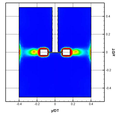
39 The first is controlled by the macro turbulence while the last two are controlled by the micro- turbulence. Studies in the past have shown that the collision rate between particles and bubbles depend on the maximum value of the dissipation rate which can be calculated from the turbulence models through out the simulations. 2.3 Configuration and parts of the Dorr-Oliver flotation cell The Dorr-Oliver stirring tank is a cylindrical tank with a conical lower part (Figure 2.1) which is agitated by a six-blade (Figure 2.2) impeller. Unlike stirring tanks employed in chemical industry, the impeller is positioned at the bottom of the tank, with very little clearance. A stator (Figure 2.3) is mounted also at the bottom of the tank. Simulations were carried out for two different elevations of the impeller with and without the stator in order to predict the effects in the flow field and in the turbulence characteristics. The parameters of the cases chosen are given in Table 2.1 Table 2.1: Simulation Matrix for the Dorr-Oliver Tank Re=35000 Distance of the impeller from the bottom of the tank Without Stator With Stator 3cm 1-1cm

40 Figure 2.1: Configuration of the Dorr-Oliver Stirring Tank Figure 2.2: Dorr-Oliver Impeller 27

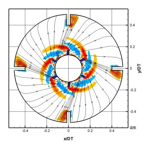
41 Figure 2.3: Dorr-Oliver Stator 2.3 Results Figure 2.4 shows the contour plots of the normalized velocity magnitudes superimposed with streamlines for the three different cases. The first two cases correspond to two different elevations of the impeller from the ground. In the third case, we added the stator shown in Fig 2.3. In the first two cases we observe that two recirculation regions form while in the last case with the stator we have only one. In addition, in the case where the impeller is closer to the bottom of the tank we can see that the stagnation points have moved from the inclined wall closer to the bottom of the tank. This may be a desirable feature for flotation processes, because more turbulence is generated with higher dissipation rate which is directed towards the floor of the tank, and thus can lift particles that may have settled there. The collision rate of bubbles and particles depends on the maximum dissipation (usually occurring in the discharge zone of the impeller) which means the higher the dissipation, the higher the collision rate. Therefore more particles will attach to the surface of the rising bubbles and will not settle in the bottom of the tank. Thus, the configuration with the impeller closer to the bottom of the tank will scrape the floor better and as a result the flotation process will be more efficient. On the other hand, in the case where the stator is present, the flow field is completely different. First of all no stagnation points exist and the streamlines indicate that the flow instead of following the tank wall while ascending, and returning back along the center, they do the opposite. This 28

42 means that the flow is going mostly upwards along the center of the tank, thus reinforcing flotation. 29

43 Figure 2.4: Contour Plots of the normalized velocity magnitude using the Standard k-ε model for the three configurations Figures 2.6 presents the contour plots of the normalized radial velocity in the impeller blade plane. From all the figures it can be observed that the radial jet is more energetic in the case where the impeller is further up. This was expected because the more flow comes in from the bottom the more will come out. Thus the case with the stator is expected to have the smaller radial component because not only is closer to the bottom but it is blocked in the periphery too. 30

44 31

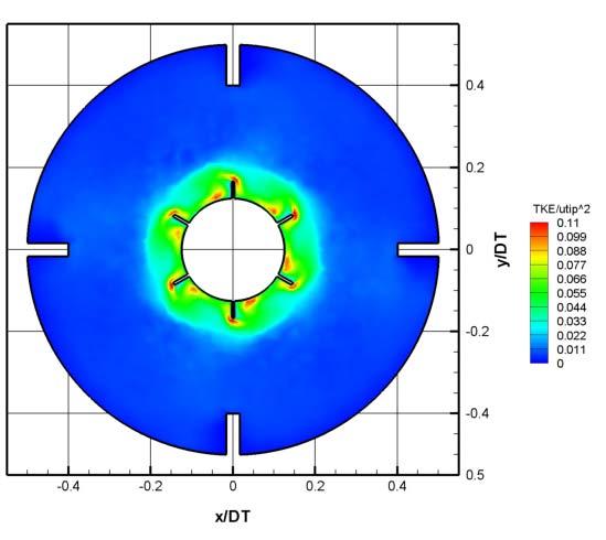
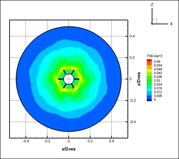
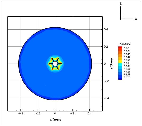
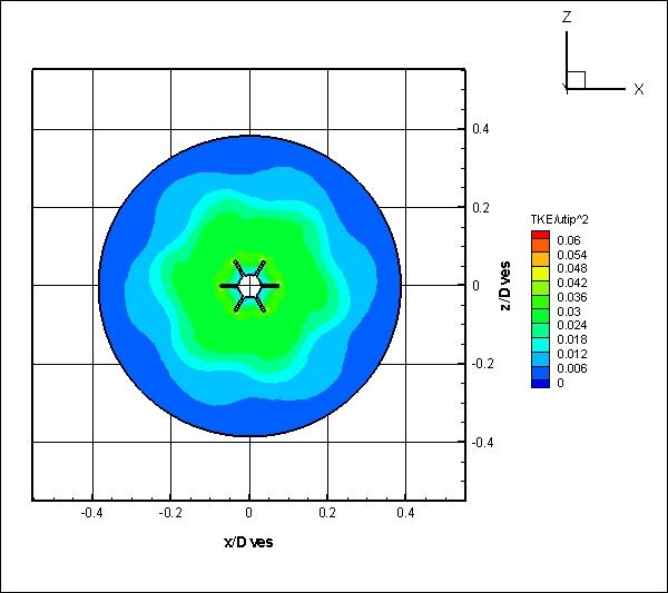
45 Figure 2.5: Contour Plots of the radial velocity using the Standard k-ε model for the three configurations (impeller blade plane) We observe that the closer the impeller is to the floor of the tank, more turbulence is generated. We attribute this to the blockage of the return flow to the impeller. With a flat disk blocking the return of the flow on the top of the impeller and the ground blocking the return form the bottom, the edges of the impeller produce slower flow but much higher levels of turbulence. In the case where the stator is present even more turbulence is generated and not only inside the stator but outside too. (Orange zones at the end of the stator indicate a high TKE). Probably this is happening because vortices form around the stator blades, and these break down to turbulence. Similar behavior is observed in the dissipation rate shown in Figure 2.7. The only difference is that even if high values of dissipation can be seen around the stator, the maximum is observed inside the stator blades. In those regions there is a high probability of collisions between particles and bubbles which could lead to more efficient flotation. 32

46 Figure 2.8 shows the non-dimensional Z-vorticity for all the tested configurations, along a plane passing through one of the impeller blades. It can be seen that the stator has a huge effect on the flow pattern. In the first two cases two distinct recirculation regions form while in the latter one small structures seem to appear between the stator blades and some inside the stator but clearly smaller than in the other cases. Figure 2.9 provides more information about these structures along a plane between the rotor blades. 33

47 Figure 2.6: Contour Plots of the normalized TKE using the Standard k-ε model for the three configurations (impeller blade plane) 34

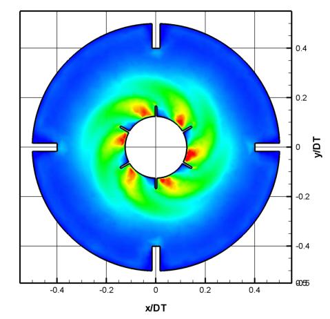
48 35

49 Figure 2.7: Contour Plots of the normalized Dissipation rate using the Standard k-ε model for the three configurations (impeller blade plane) 36

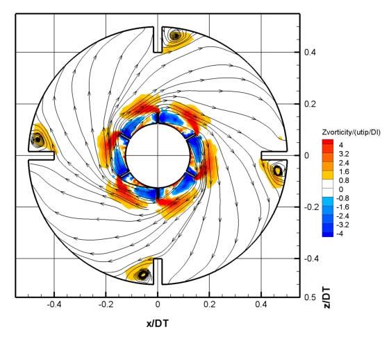
50 Figure 2.8: Contour Plots of the normalized Z-vorticity using the Standard k-ε model for the three configurations. 37

51 38

52 Figure 2.9: Contour Plots of the normalized Z-vorticity using the Standard k-ε model for the three configurations in a plane between the rotor blades ( / 0 x Dves = ) Figures 2.10, 2.11 and 2.12 show the streamlines of all the configurations along three different horizontal cut-planes of the impeller, namely at y/ H imp = 1/ 4, y/ H imp = 1/2 and at y/ H imp = 3/ 4. The minus (-) sign indicate that these planes are below the impeller disk which has been defined as the zero (0) elevation. In Figure 2.10 in the first case the turbine pushes all the fluid out. In the second case in which the impeller has been moved closer to the bottom of the tank we notice again that most of the fluid is directed out but a distinct circle can be seen. This is the envelope of the streamlines separating those that spiral inward from those that spiral outward. Lastly, in the case with the stator, the fluid in its effort to pass through the stator blades form small vortices between them, while some of the fluid is returning back as it was indicated in Figure 2.4. As we proceed to next slice which is located in the middle of the impeller (Figure 2.11) in the first two cases we can observe that some of the flow is returning back from the two recirculation regions next to the impeller while some of it is still going out (on the opposite 39

53 direction in the big recirculation region). In the case of the low clearance (1cm from the bottom of the tank) the inside circle is smaller. This is due to the fact that the vortices do not extend as much as in the other case. On the other hand, in the case with the stator the streamlines do not merge as before to create a circle. Therefore most of the flow is returning back from the huge recirculation region (outside from the stator) while some of it inside the stator still tries to pass through. Finally in Figure 2.12 (one forth from the bottom of the tank) the circle for the first two cases grows because more flow is returning back to the impeller. The same behavior is observed in the case in which we have the stator. This can be explained because in the lower part of the tank, instead of sixteen stator blades there are only four and therefore they do not block as much the flow as at the higher elevations 40

54 Figure 2.10: Streamlines using the Standard k-ε model for all three configuration in a horizontal slice that passes through the first one forth of the impeller ( y/ H imp = 1/ 4 ) 41

55 42

56 Figure 2.11: Streamlines using the Standard k-ε model for all three configuration in a horizontal slice that passes through the middle of the impeller ( y/ H imp = 1/ 2 ) 43

57 Figure 2.12: Streamlines using the Standard k-ε model for all three configuration in a horizontal slice that passes through the last one forth of the impeller ( y/ H imp = 3/4) 44

58 In Figure 2.13 in the first case we can notice that vorticity is high around the impeller blade where an extended vortex is formed as we saw in Figure 2.8. The second vortex (the big one) starts further up and cannot be captured very well in this slice. As far as the second case is concerned, the small vortices are very close to impeller blades and the second one starts closer. This is why high values of vorticity are extended further away (orange-yellow zones). The outside recirculation regions are not as spinning as violently as the inner, so no red values (the highest values based on the color zones) are observed. In the case of the stator/rotor configuration high values of vorticity can be observed everywhere due to the vortices that form around the stator blades. Figure 2.14 indicates that high values of vorticity still exist but they do not extend too much further out. In the case with the stator, higher values are observed next to rotor blades than in the stator blades. This can be attributed to the fact that now more flow is moving inward than outward, and therefore the impeller makes a bigger effort to push the flow outside. Lastly in Figure 2.15 although we observe the same behavior for the first two cases with even less high values of vorticity as we move further away from the impeller in the case with the impeller no higher vorticity values can be seen. This is due to the lower number of the stator blades as we mentioned before. Only four stator blades are present, and therefore the flow is not so much interacting with them. 45

59 46

60 Figure 2.13: Normalized Y-vorticity using the Standard k-ε model for all three configuration in a horizontal slice that passes through the first one forth of the impeller ( y/ H imp = 1/ 4 ) 47

61 Figure 2.14: Normalized Y-vorticity using the Standard k-ε model for all three configuration in a horizontal slice that passes through the first one forth of the impeller ( y/ H imp = 1/ 2 ) 48

62 49

63 Figure 2.15: Normalized Y-vorticity using the Standard k-ε model for all three configuration in a horizontal slice that passes through the first one forth of the impeller ( y/ H imp = 3/ 4 ) Figures 2.16, 2.17 and 2.18 illustrate the normalized Turbulent Kinetic Energy (TKE) for all the studied cases in three different elevation slices. Figure 2.16 demonstrates that the configuration which has the impeller further up from the bottom of the tank has the lowest TKE. The flow is only directed outwards in that case. In the second case where the impeller is closer to the bottom generates more turbulence and therefore more TKE. Finally, when the stator is added the flow finds more resistant, creates vortices around it and higher values of TKE can be observed inside and outside the stator blades. Figure 2.17 shows that the TKE for the first case increased while in the second the opposite happened. In the case with the stator it decreased in the boundary of it but increased in the area close to the rotor blades. As we mentioned before more flow is coming in than going out which results to happen the above phenomenon. Lastly, Figure 2.19 indicates that low values of TKE are dominated in the first two configurations while in the one with the stator higher values of TKE than before appear next to the impeller blades. 50

64 51

65 Figure 2.16: Normalized TKE using the Standard k-ε model for all three configuration in a horizontal slice that passes through the first one forth of the impeller ( y/ H imp = 1/ 4 ) 52

66 Figure 2.17: Normalized TKE using the Standard k-ε model for all three configuration in a horizontal slice that passes through the first one forth of the impeller ( y/ H imp = 1/ 2 ) 53

67 54

68 Figure 2.18: Normalized TKE using the Standard k-ε model for all three configuration in a horizontal slice that passes through the first one forth of the impeller ( y/ H imp = 3/ 4 ) Figures demonstrate the non-dimensional dissipation for the studied cases in the three different elevation slices. The conclusions which somebody can draw follow the ones for the TKE. Figure B.22 shows the normalized Y-vorticity isosurfaces for the studied cases. 55

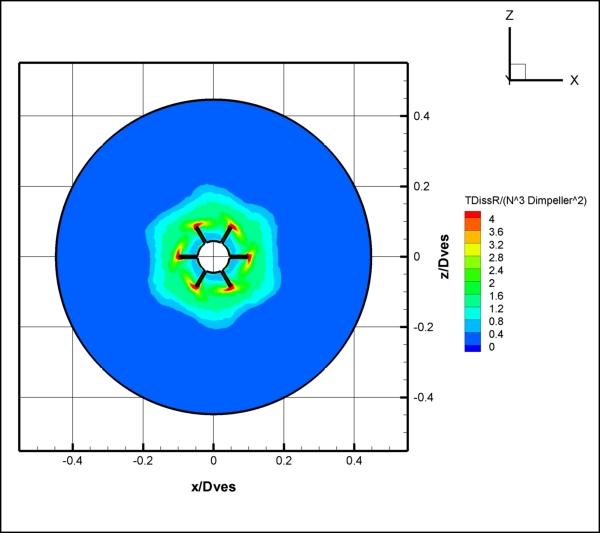
69 56

70 Figure 2.19: Normalized Dissipation rate using the Standard k-ε model for all three configuration in a horizontal slice that passes through the first one forth of the impeller ( y/ H imp = 1/4) 57

71 Figure 2.20: Normalized Dissipation rate using the Standard k-ε model for all three configuration in a horizontal slice that passes through the first one forth of the impeller ( y/ H imp = 1/2) 58

72 59

73 Figure 2.21: Normalized Dissipation rate using the Standard k-ε model for all three configuration in a horizontal slice that passes through the first one forth of the impeller ( y/ H imp = 3/4) 60

74 Figure 2.22: Normalized Y-isovorticity using the Standard k-ε model for all three configurations 61

75 CFD simulations were carried out for three different configurations with the Standard k-ε turbulence model and for Re=35000 in order to investigate the effect of the clearance and the stator on the velocity field. In the first two configurations chosen, the impeller was placed at two distances from the floor of the flotation cell, namely at 1cm and 3cm but the stator was removed. In the third case a full stator configuration was added for a clearance of the impeller of 1cm from the bottom of the tank. The flow field without the stator looks similar for both clearance cases; two recirculation regions can be observed. In case of the low clearance configuration, namely, at 1cm from the bottom of the tank, the impeller jet attaches on the floor of the tank. Since the impeller jet convecting turbulent structures, we conjecture that attachment on the floor involves scraping and therefore agitating and lifting particles that tend to settle by gravity. In the case with the stator the flow field is completely different. No stagnation points exist and the flow is mostly directed upwards in the middle of the tank, reinforcing flotation. Two small vortices form between the edge of the disk that forms a barrier on top of the impeller and the stator ring. This is because of the jet that is generated from every passage of the impeller which impinges on the stator ring. Our simulations indicate that the presence of the stator creates more turbulence. High values of turbulent kinetic energy and dissipation rate can be seen in the immediate neighborhood of the stator. This is due to the vortices that form between the stator blades. In order to analyze in greater detail the changes that occur in the neighborhood of the impeller region, we cut three horizontal slices at three elevations of the impeller, namely, one third, one half and three forths ( y/ H imp = 3/ 4 ) of impeller diameters below the cover of the impeller. From these contour plots we can draw the conclusion that the higher values of the turbulent kinetic energy and the dissipation rate are observed in the first plane ( y/ H imp = 1/ 4 ) because more flow is directed outwards and at a higher speed, than inwards and it finds more resistance from the stator blades. In the lowest plane ( y/ H imp = 3/ 4 ) due to the fact that all the flow is entering the impeller domain the impeller makes greater effort to push the flow outside. The point is that a rotating blade tends to move fluid radically outward. But in the present situation, the top of the impeller is blocked by the circular roof plate of the impeller and the bottom is blocked by the floor of the tank. Therefore, with a strong centrifugal action on the top where 62

76 the impeller blades have a larger diameter, the flow exits the impeller domain thee and thus it is forced into the impeller domain lower. In this region therefore, the blades tend to move the flow outward conservation of mass forces it inward. To conclude, the presence of the stator plays an important role in the flotation process because more turbulence is generated which means that the values of the maximum dissipation rate are larger and are located inside the stator and very close to the impeller outflow. Therefore the collision rates between air bubbles and particles is larger (more particles will attach to the air bubbles and will float) and as a result the flotation process will be more efficient. Moreover, the bubble/particle aggregates will find a mild upward flow motion in the middle of the tank, which will improve the flotation process. In all other cases studied the recirculation patterns involve downward motions in the middle of the tank, which would tend to oppose the flotation process. 63

77 APPENDIX I RUSHTON TURBINE A. Outline of turbulence models for the stirring tank simulations i. The Two- Equation k-ε Models Among the existing turbulence models the family of the two equation k-ε models is the most simplest to use. The purpose of these models is to predict an eddy viscosity. A k-ε model consists of two equations; one for the Turbulent Kinetic Energy (TKE) and one for the dissipation rate (ε). At high Reynolds numbers the rate of dissipation and the production (P) are of similar order of magnitude. Therefore, we estimateε P.This correlation implies that once Turbulent Kinetic Energy is generated at the low wave number end of the spectrum (large eddies) it is immediately dissipated at the same location at the high wave number end (small eddies). [11] a. The Standard k-ε Model The Standard k-ε model was initially developed by [25] and was the first two-equation model used in applied computational fluid dynamics. This model is based on the Boussinesq hypothesis (isotropic stresses) that the Reynolds stress is proportional to the mean velocity gradient, with the constant of proportionality being the turbulent or eddy viscosity. The equation for the turbulent viscosity ( ν turb ) is given by: 2 k ν t = c µ (I.1) ε Where k is the kinetic energy, ε is the dissipation rate and c µ is a parameter that depends on the k-ε turbulence model. In this case is equal to c µ =

78 The Turbulent Kinetic Energy (TKE) for three dimensional flows is given by: 1 '2 '2 '2 k = ( u + v + w ) (I.2) 2 This model became a workhorse for many engineering application because it combines reasonable accuracy, time economy and robustness for a wide range of turbulent flows. The governing transport equations for this model can be written as: k-equation: ε- equation: ( ) ( ) ( ) ρk ρuk ρ uk µ k t x x x ( P ε ) i i t + = + ρ i i σ k i ( ) ( u ) ( uk) ρε ρ iε ρ i µ t ε 1 + = + ρ t xi xi σε xi τd ( c1, εp c2, εε ) In the above equations τ d is the dissipation rate time scale that characterizes the dynamic process in the energy spectrum and P is the production for turbulence. The equations of these terms are given by: k τ d = (I.5) ε P u u u i j j = vt + x j x i xi The empirical constants c µ, c k, c ε, c 1, ε, c2, ε,are given in Table A.1 (I.3) (I.4) (I.6) Table I.1: Parameters for the Standard k-ε model Model Parameters c µ = 0.09 σ = 1 σ = c1, ε = 1.44 c2, ε = 1.92 k ε b. The RNG k-ε Model The RNG k-ε model is one of the most popular modifications. It has become known due to some weakness of the Standard k-ε. It was derived from the Standard k-ε using the 65

79 renormalization group theory (a statistical method) in order to be more accurate in rapidly strained and swirling, flows. This theory is first used to resolve the smallest eddies in the inertial range. After resolving these small eddies a small band of the smallest eddies is eliminated by representing them in terms of the next smallest eddies. This process continues until a modified set of the Navier Stokes equations is obtained which can be solved using even a coarse grid. Changes have been made deriving a formula for the effective viscosity that accounts for low Re number effects as well. The governing equations for the RNG k-ε model are: k-equation: ε-equation: eff ( ρ ) ( ρ ) ( ρ ) k uk i uk i k + = akµ eff + ρ ε t xi xi xi ( ) ( u ) ( uk) ( P ) ρε ρ ε i ρ i 1 a ε + = εµ eff + ρ c εp c εε t xi xi xi τ d t * ( 1, 2, ) µ = µ + µ (I.9) c η η 1 η = c 1+ β η * 0 1, ε 1, ε 3 (I.7) (I.8) (I.10) S k η = (I.11) ε S = 2 Sij Sij (I.12) The main difference between the Standard k-ε model and the RNG k-ε is the additional sink term in the ε equation (second term in equation (I.8)) The empirical constants for this modelc µ, σ, σ ε, η 0, β, c 1, ε, c2, ε are given in Table I.2 k Table I.2: Parameters for the RNG k-ε model Model Parameters c µ = α = 1.39 α = 1.39 η 0 = 4.38 β = c1, ε = 1.42 c2, ε = 1.68 k ε 66

80 c. The Realizable k-ε Model This model is relatively new and differs from the Standard k-ε model because it contains a new form for the ν turb and a new transport equation for the ε derived from an exact equation for the transport of the mean square vorticity fluctuations. The term realizable means that it consistent with the physics of turbulence (mathematical constraints on the Reynolds stresses). One disadvantage of this model is that when a multi reference frame (MRF) or a sliding mesh (SM) are used it produces non-physical turbulent viscosities due to the fact that includes the mean rotation effects in the ν turb equation. Thus, the use in the above frames should be taken with some caution. In this case c µ is no longer a constant but is given from the following equation: c µ 1 = * ku Ao + As ε which in its turn consist of some other parameters as follows: (I.13) As = 6 cosϕ (I.14) 1 cos 1 ( 6 W ) ϕ = (I.15) 3 SSS ij ij ki W = (I.16) 3 S S = S S (I.17) ij ij U * = S S +Ω Ω (I.18) ij ij ij ij Ω =Ω 2e ω =Ω e ω (I.19) ij ij ijk k ij ijk k Ω is the mean rate of the rotation tensor presented in a rotation frame with angular velocityω ij and Sij is given by k S ij 1 u u i j = + 2 x j x i 67 (I.19a)

81 The model parameters A, σ k, σ ε, c 1, ε, c2, ε are given from Table I.3 Table I.3: Parameters for the Realizable k-ε model Model Parameters σ = 1 σ = 1.2 A = 4.04 c1, ε = 1.44 c2, ε = 1.92 k ε ii. A Seven Equation k-ε Model a. The Reynolds Stress Model (RSM) The Reynolds Stress Model also referred to as the Reynolds stress transport is more general but more complex comparing to other turbulence models for time-averaged calculations implemented in many commercial CFD packages. This model consists of six transport equations for the Reynolds stresses uu ' and an equation for the dissipation rateε. The Reynolds stress transport equation is given as follows: ' ' ( ) D uu + T = P + R ε Dt i j kij ij ij ij xk where the terms in the left and right hand side of the above equation are explained here: D ' ' Local Time Derivative: ( uu i j) T T T T kij kij kij Dt i ' j (I.20) (I.21) u v p kij = + + (I.22) Convection Tensor: T = u uu (I.23) u ' ' kij k i j Molecular Diffusion Tensor: T v kij = ν 1 ρ ' ' ( uu i j) x p ' ' ' Turbulent Diffusion Tensor: Tkij = uu i juk + p( uiδ jk + ujδik ) k (I.24) (I.25) u ' ' j ' ' Production Tensor: Pij = uu i k + ujuk xk ui x k (I.26) 68

82 Pressure-rate of strain Tensor: R ij ' ' p u u i j = + ρ uj u i (I.27) ' ' Dissipation Tensor: ε i j ij 2 ν u u = (I.28) xk x k The convection, the molecular diffusion and the production terms are in closed forms due to the fact that they contain only the dependent variable uu ' ' and mean flow gradients so they don t need to be modeled. However, modeling of the turbulent diffusion, the pressure-strain and the dissipation rate (calculated from ε equation) are required. Although as we said it is more general model than the two equation models it is computationally time consuming because it consists of seven equations for the turbulence modeling. This model allows the development of anisotropy, or orientation of the eddies in the flow. Therefore, has good accuracy in predicting flows with swirl, rotation and high strain rates. i j B. Grid Study In this section results from a grid study of three different grids and three turbulence models are presented. All the grids were unstructured and were generated in the commercial package GAMBIT. The coarse, fine and the finest grid had 220,000, 350,000 and 480,000 elements respectfully. With the Reynolds stress model only the finest grid was tested, due to the fact that it consists of seven equations instead of two and it needs better resolution because it accounts for anisotropy. As it can be seen from the Figure I.1 as the grid size becomes finer results tend to be closer to the experimental data. In the case of the turbulent kinetic energy (Figure I.2) all the models with all the grids underpredicted the experimental results. We also observed that even the Reynolds stress model gave poor results. As far as the dissipation is concerned (Figure I.3), only the finest grid of the RNG k-e gave good results, even in the area next to the blade were the steepest gradients are present and the Reynolds stress models should have superior behavior, again because it accounts for anisotropy. 69

83 Finest grid using the K-e model Fine grid using the K-e model Coarse grid using the K-e model Finest Grid using the RNG K-e model Fine grid RNG K-e model Coarse grid RNG K-e model Finest grid using the Reynolds Stresses Experimental results Vr/Utip r/dtank Figure I.1: Normalized radial velocity at the centerline of the impeller for all the grids and turbulence models Finest grid using the K-e model Fine grid using the K-e model Coarse grid using the K-e model Finest Grid using the RNG K-e model Fine grid RNG K-e model Coarse grid RNG K-e model Finest grid using the Reynolds Stresses Experimental results TKE/(Utip 2 ) r/dtank Figure I.2: Normalized TKE at the centerline of the impeller for all the grids and turbulence models 70

84 Finest grid using the K-e model Fine grid using the K-e model Coarse grid using the K-e model Finest Grid using the RNG K-e model Fine grid RNG K-e model Coarse grid RNG K-e model Finest grid using the Reynolds Stresses Experimental results ε/(n 3 Dimp 2 ) r/dtank Figure I.3: Normalized Dissipation rate at the centerline of the impeller for all the grids and turbulence models C. CFD Simulations of a Rushton tank and a flotation cell CFD simulations were carried out for the geometry of a stirring tank adopted for a parallel experimental study. This consisted of a small-scale cylindrical stirring vessel made of Plexiglas with diameter D T =0.1504m (shown in Figure I.4). Four equally-spaced axial baffles with width (w b ) one tenth of the tank diameter were mounted along the wall. The tank was closed at the top, and was filled with deionized water as the working fluid. A Rushton impeller used to agitate the fluid was located at a height m from the bottom. (in the middle of the tank). The ratio between the vessel and the impeller diameter was D imp/ D T =1/3.The ratio of blade width (w i ) to the impeller diameter (D imp ) was The height of the water was maintained at m, which is equal to the tank diameter. The cylindrical tank was housed in an outer rectangular tank filled with water to eliminate the optical distortion of light beams passing through a curved boundary of media with different indices of refraction. 71

85 The region most interesting in the above configuration is the region immediately adjacent to the impeller. We chose this region because of the extreme increase in velocities and turbulent statistics from the rest of the tank. For this reason CFD calculations for Re number equal to are performed to check how the results with different turbulence models are compared with those from the Experiments. z r (a) (b) Figure I.4: Stirring Tank configuration: (a) Three dimensional and (b) Cross sectional view of the Tank D. The Multi-Reference System This report discusses the application of different turbulence models in a stirring tank equipped with a Rushton impeller. Although that better numerical techniques and increasing computational power permits unsteady simulations, there is a wide range of applications that require steady-state calculations such as biotechnological and chemical reaction where other physical phenomena are involved. Therefore, a Multi Reference System (MRF) is applied for calculating time averaged velocities and other turbulence quantities. As mentioned earlier this model allows the flow simulation in baffled stirring tanks with rotating or stationary internal parts. It uses at least two frames, one containing the frame where moving or rotating parts 72

86 (impellers, turbines) are present and another one for the stationary regions. The first is rotating with the impeller and thus in this frame of reference the impeller is at rest. The second one is stationary. We mentioned that MRF could involve at least two frames, but it can have multiple frames in case where stirring tanks with multiple turbines have to be simulated. With this approach several rotating frames can be modeled while the remaining space can be modeled as stationary. The momentum equations inside the rotational frame are solved in the unsteady form while those outside the rotating frame are solved in a steady form. In Figure I.5 a plot of the 3D stirring tank grid with the two frames of reference are presented. The green area is the rotating frame of reference that encloses the Rushton turbine while the white one is the stationary frame. The rotational frame of reference has Diameter 1.2 times the Diameter of the impeller. Figure I.5: Computational Grid for simulations with the MRF model 73

87 E. Non Dimensional numbers A number of dimensionless parameters that are important for the flow in stirring vessels are presented. a. The Reynolds number One of the most common but important dimensionless parameter is the Reynolds number (Re). It controls the scale of the model and the corresponding flow velocities. It characterizes the region of the flow as laminar, transitional and turbulent. It is defined as the ratio of the inertial forces to viscous forces and is given by the following equation: ρud ud Re = = (I.29) µ ν where u is the characteristic velocity and D is the characteristic diameter. In the case of stirring tanks D is the diameter of the impeller and u is the tip velocity of the blade. The tip velocity is given by: D utip = ωr = 2πN = πdn (I.30) 2 where N is the rotational speed of the impeller. Usually in the literature before substituting (A.30) into (A.29) investigators drop the π in the u tip. Therefore, the Re number is finally given by: 2 ND Re = (I.31) ν Depending on the problem the region where the flow is laminar, transitional or turbulent is different. For example for pipe flow the flow is laminar when Re<2000, transitional for 2000<Re<4000 and turbulent for numbers larger than In stirring tanks the flow is laminar for Re<50 transitional 50<Re< 5000 and fully turbulent for Re> But this still depends on the power number of the impeller. 74

88 b. Power Number The power number parameter is defined by the ratio of the drag forces applied to the impeller to the inertial forces and is given by: P Po = (I.32) 3 5 ρ ND The Power delivered to the fluid can be calculated straight out from the CFD calculations or from the following equation: P= π NF (I.33) 2 torque The torque can be calculated by integrating the Pressure on the impeller blade. A ( τ ) Ftorque = ω r da (I.34) There is a relation in the CFD packages from which the Power number can be obtained: 5w b N Po a b = D 6 b abare, constants (5, 0.8), D is the impeller diameter w b is the width of the blade and (I.35) N b is the number of blades. Our Rushton turbine has: N = 6 with w = m. By substituting them into (I.35) we obtain: Po = 6.25 The above number is correct assuming unbaffled tank. In case where baffles are present the power number is significantly affected. Figure (I.7) shows the effect of baffles on the power number for different impeller sizes. wb D In our case: Nb = 0.4 and = 0.33 thus 1.05 T T Po =. To conclude, we can say that the power number for a single impeller depends on the impeller type, the size of the impeller comparing to the size of the tank, the Re number, the elevation of the impeller, the number of baffles and their width if any are present. b b 75

89 c. Froude Number The Froude number is defined as the ratio of inertial forces to gravitational forces and it is given by: u N D N D Fr = = = (I.36) Dg Dg g The Froude number is an important parameter for studying the motion of vortices in unbaffled tanks. Although the effect of the Froude number is negligible for baffled tanks or unbaffled with Re<300, for unbaffled with Re>300 we can define a new function (I.37) that contains both the Po and the Fr non-dimensional numbers f = b Po ( a log Re) Fr (I.37) By plotting f as a function of Re number we get a line similar to the one that relates the Po number with the Re number. d. Flow number The Flow number (Fl) is a parameter that characterizes the pumping capacity of an impeller and it can be defined as: Q Fl = (I.38) 3 ND Q can be calculated by integrating the outflow in the discharge area of the impeller. For axial impellers the area is circular while for the radial ones it is a section of a cylinder. The Flow number for a radial disk impeller can also be calculated theoretically from the following equation: Nb wblade D Fl = a 6 D T a = 6 b = 0.7 c = 0.3 b c (I.39) 76

90 The values of the constants a, b, c can be modified Figure I.6: Power Number versus Re number Figure I.7: Effect of the baffles and impeller size on the Po number 77

91 F. More results concerning the Rushton turbine In the main body of the dissertation we present the most basic results that will be needed for an archival publication. In this section additional results for the case of the Rushton tank can be found. More specifically non-dimensional line plots of radial and tangential velocity, velocity magnitude, dissipation rate, turbulent kinetic energy and vorticity at the centerline of the impeller are presented for three Re numbers (20000, and 45000). Figure I.8 illustrates the predicted profiles of the radial velocity and the velocity magnitude at the impeller radial center line for all the tested turbulence models, as well as the in-house experimental data measured via Digital Particle Image Velocimetry (DPIV). It can be seen that the Standard k-e model predicts quite well the maximum values. As we move radically further from the impeller until the point r/ D = 0.27, it underpredicts them, and beyond that point the Standard k-e model results agree relatively well with the experimental data. The RSM model in this case gives the poorest results from all the turbulence models. The RNG K-e overpredicts the experimental results near the impeller but further out into the filed it agrees very well with the experiment. In-house experimental data are not available for the other two cases of impeller clearance. Especially for the low clearance configuration experimental results do not exist in the literature at all. We observe that the radial component of the velocity for this case is very small compared to the other two configurations. In the bottom frame when we present the velocity magnitude we have calculated only the root of the sum of the squares of two (radial and axial) of the three components of the velocity in order to compare it with the experimental data. Measurements have been taken in a perpendicular plane that passes through the impeller blades and therefore no out of plane component (circumferential) is available. tan k 78

92 CFD results using the K-e model for C/T=1/2 CFD results using the RNG K-e model for C/T=1/2 CFD results using the Reynolds Stresses for C/T=1/2 Experimental results for C/T=1/2 CFD results using the K-e model for C/T=1/3 CFD results using the K-e model for C/T=1/ Vr/Utip r/dtank CFD results using the K-e model for C/T=1/2 CFD results using the RNG K-e model for C/T=1/2 CFD results using the Reynolds Stresses for C/T=1/2 Experimental results for C/T=1/2 CFD results using the K-e model for C/T=1/3 CFD results using the K-e model for C/T=1/15 Vmgn/Utip r/dtank Figure I.8: Normalized radial velocity (top frame) and velocity magnitude (bottom frame) at the centerline of the impeller for all the three different configurations for Re=

93 Comparisons for the dissipation rate and the turbulent kinetic energy are shown in Figure I.9. All the turbulence models overpredict the dissipation rate close to the impeller blades. This happens because in that area we have the steepest gradients which make the calculations more complex. A little further from the impeller tip the values of the dissipation drop sharply. The model that captures most details in that case is the RNG K-e. As far as the turbulent kinetic energy is concerned all the turbulence models underpredict its value, mostly at the impeller discharge zone. This can be explained by the fact that the experimental results contain contributions from the periodic motion of the impeller blades, since every time a blade passes by the point of interest; a strong radial jet is created. In the literature it is stated [14] that by removing (filtering) that periodicity, the values of turbulent kinetic energy drop and in most cases would have matched computational results. Figure I.9 confirms the idea that experimental values result following this procedure, but there is sill some discrepancy with the calculated results. Although the Reynolds stress model is the one that is closer to the experimental results without the periodicity, it still underpredicts them. 80

94 CFD results using the K-e model for C/T=1/2 CFD results using the RNG K-e model for C/T=1/2 CFD results using the Reynolds Stresses for C/T=1/2 Experimental results for C/T=1/2 CFD results using the K-e model for C/T=1/3 CFD results using the K-e model for C/T=1/15 ε/(n 3 Dimp 2 ) r/dtank CFD results using the K-e model for C/T=1/2 CFD results using the RNG K-e model for C/T=1/2 CFD results using the Reynolds Stresses for C/T=1/2 Experimental results for C/T=1/2 with periodicity Experimental results for C/T=1/2 without periodicity CFD results using the K-e model for C/T=1/3 CFD results using the K-e model for C/T=1/15 TKE/(Utip 2 ) r/dtank Figure I.9: Normalized dissipation rate (top frame) and turbulent kinetic energy (bottom frame) at the centerline of the impeller for all the three different configurations for Re=

95 The top frame of Figure I.10 displays the distribution of the vorticity along the centerline of the impeller. Clearly none of the turbulence models can capture what is happening. Every time that a blade is passing a strong radial jet is created followed by the trailing vortices that propagate downstream as indicated from the experimental results. The nature of the vorticity seems to have this oscillating behavior in the experiments due to the periodicity and due to the fact that trailing vortices is present. It may also be possible that the method of calculating vorticity from the measured velocity components introduces errors. The bottom frame of the same figure compares the tangential velocities at the impeller centerline. What is shown in this Figure agrees with the theory in the sense that the tangential component of the velocity has high absolute values close to the impeller, and as we move radically out takes smaller values. Unfortunately in-house experimental results are not available, and it is difficult to compare them with results from the literature because different configurations and different Reynolds number are available. Figures I.8 to I.10 correspond to Re= Figures I.11-I.13, I.14-I.15 show similar profiles for all the studied variables (radial velocity, velocity magnitude, tangential velocity, turbulent kinetic energy, vorticity and dissipation rate) for different Reynolds numbers, namely and The results are qualitatively similar to those obtained at Re=

96 5 4 3 CFD results using the K-e model for C/T=1/2 CFD results using the RNG K-e model for C/T=1/2 CFD results using the Reynolds Stresses for C/T=1/2 Experimental results for C/T=1/2 CFD results using the K-e model for C/T=1/3 CFD results using the K-e model for C/T=1/15 Vorticity/(Utip/Dimp) r/dtank Vtheta/Utip CFD results using the K-e model for C/T=1/2 CFD results using the RNG K-e model for C/T=1/2 CFD results using the Reynolds Stresses for C/T=1/2 Experimental results for C/T=1/2 CFD results using the K-e model for C/T=1/ r/dtank Figure I.10: Normalized X-vorticity (top frame) and tangential velocity (bottom frame) at the centerline of the impeller for all the three different configurations for Re=

97 CFD results using the K-e model for C/T=1/2 CFD results using the RNG K-e model for C/T=1/2 CFD results using the Reynolds Stresses for C/T=1/2 Experimental results for C/T=1/2 CFD results using the K-e model for C/T=1/3 CFD results using the K-e model for C/T=1/ Vr/Utip r/dtank CFD results using the K-e model for C/T=1/2 CFD results using the RNG K-e model for C/T=1/2 CFD results using the Reynolds Stresses for C/T=1/2 Experimental results for C/T=1/2 CFD results using the K-e model for C/T=1/3 CFD results using the K-e model for C/T=1/15 Vmgn/Utip) r/dtank Figure I11: Normalized radial velocity (top frame) and velocity magnitude (bottom frame) at the centerline of the impeller for all the three different configurations for Re=

98 CFD results using the K-e model for C/T=1/2 CFD results using the RNG K-e model for C/T=1/2 CFD results using the Reynolds Stresses for C/T=1/2 Experimental results for C/T=1/2 CFD results using the K-e model for C/T=1/3 CFD results using the K-e model for C/T=1/15 ε/(n 3 Dimp 2 ) r/dtank CFD results using the K-e model for C/T=1/2 CFD results using the RNG K-e model for C/T=1/2 CFD results using the Reynolds Stresses for C/T=1/2 Experimental results for C/T=1/2 with periodicity Experimental results for C/T=1/2 without periodicity CFD results using the K-e model for C/T=1/3 CFD results using the K-e model for C/T=1/15 TKE/(Utip 2 ) r/dtank Figure I.12: Normalized dissipation rate (top frame) and turbulent kinetic energy (bottom frame) at the centerline of the impeller for all the three different configurations for Re=

99 CFD results using the K-e model for C/T=1/2 CFD results using the RNG K-e model for C/T=1/2 CFD results using the Reynolds Stresses for C/T=1/2 Experimental results for C/T=1/2 CFD results using the K-e model for C/T=1/3 CFD results using the K-e model for C/T=1/15 Vorticity/(Utip/Dimp) r/dtank Vtheta/Utip) CFD results using the K-e model for C/T=1/2 CFD results using the RNG K-e model for C/T=1/2 CFD results using the Reynolds Stresses for C/T=1/2 Experimental results for C/T=1/2 CFD results using the K-e model for C/T=1/ r/dtank Figure I.13: Normalized X-vorticity (top frame) and tangential velocity (bottom frame) at the centerline of the impeller for all the three different configurations for Re=

100 CFD results using the K-e model for C/T=1/2 CFD results using the RNG K-e model for C/T=1/2 CFD results using the Reynolds Stresses for C/T=1/2 Experimental results for C/T=1/2 CFD results using the K-e model for C/T=1/3 CFD results using the K-e model for C/T=1/15 Vmgn/Utip) r/dtank Vtheta/Utip) CFD results using the K-e model for C/T=1/2 CFD results using the RNG K-e model for C/T=1/2 CFD results using the Reynolds Stresses for C/T=1/2 CFD results using the K-e model for C/T=1/3 CFD results using the K-e model for C/T=1/ r/dtank Figure I.14: Normalized velocity magnitude (top frame) and tangential velocity (bottom frame) at the centerline of the impeller for all the three different configurations for Re=

101 5 4 3 CFD results using the K-e model for C/T=1/2 CFD results using the RNG K-e model for C/T=1/2 CFD results using the Reynolds Stresses for C/T=1/2 Experimental results for C/T=1/2 CFD results using the K-e model for C/T=1/3 CFD results using the K-e model for C/T=1/15 Vorticity/(Utip/Dimp) r/dtank Figure I15: Normalized X-vorticity at the centerline of the impeller for all the three different configurations for Re=

102 In Figure I.16 streamlines of the fluid flow for the case where C/T=1/2 and for Re=35000 are presented in two horizontal slices that are equally spaced from the middle center plane. Their dimensionless positions are at: z/ DT = ± 0.2. The patterns are different from the middle slice where the flow was directed outwards because of the radial jet. Figure I.17 shows the dimensionless Y-vorticity in a plane that comes passes the end of the blades for Re=35000 and clearance: C/T=1/2. Two sets of positive (red) and negative (blue) vorticity are observed. Each set represents a trailing vortex that forms behind every blade, as it is better seen from the isosurfaces of vorticity in Figure I.24 Figure I16: Streamlines using the Standard k-ε model at / 0.2 z DT =± (above and below the impeller) 89

103 Figure I17: Contour Plots of the Normalized Y-vorticity using the Standard k-ε model at a plane that passes through the end of the blades for C/ T = 1/2 and Re= D view (top frame) and details (bottom frame) 90

104 In Figure I.18 (top frame) radial velocity profiles obtained by simulations, using three different turbulence models, and measurements are compared at r/t=0.19 (very close to the blades) and for Re=35000.All the turbulence models predict quite well the profile of the radial jet. The velocity is normalized with the tip velocity of the blade and the axial distance with the blade width. The second frame in this Figure shows the dissipation rate profiles again at r/t=0.19 and for Re= Either the Standard k-e model or the Reynolds stress models are able to capture the rapid changes of the dissipation rate while the RNG K-e underpredicts it. Figure I.19 and I.20 illustrate the same variables for the same Re number but in two stations further downstream from the impeller blades (r/t=0.256 and r/t=0.315). In the first case (r/t=0.256) although the velocity profiles are still well captured by all the turbulence models, the dissipation rate is overestimated by the Standard K-e and the Reynolds stress model and only a little by the RNG K-e. As we continue downstream (r/t=0.315), we observe that the profiles of the velocity obtained from the simulations start to diverge from the measurements. Although the dissipation profiles obtained by the Standard K-e and the Reynolds Stress model still overpredict the experimental data, the RNG K-e model seems to be promising. By observing the shape of the velocity profiles of the jet we see that as we go further downstream they open up as we expect from the jet theory. 91

105 2 1.5 CFD results using the K-e model for C/T=1/2 CFD results using the RNG K-e model for C/T=1/2 CFD results using the Reynolds Stresses model for C/T=1/2 Experimental results for C/T=1/ z/wbl Vr/Utip CFD results using the K-e model for C/T=1/2 CFD results using the RNG K-e model for C/T=1/2 CFD results using the Reynolds Stresses model for C/T=1/2 Experimental results for C/T=1/2 0.5 z/wbl ε/(n 3 Dimp 2 ) Figure I.18: Normalized radial velocity (top frame) and dissipation rate profiles (bottom frame) at r/t=0.19 for C/ T = 1/2and Re=35000 with all the tested turbulence models 92

106 2 1.5 CFD results using the K-e model for C/T=1/2 CFD results using the RNG K-e model for C/T=1/2 CFD results using the Reynolds Stresses model for C/T=1/2 Experimental results for C/T=1/ z/wbl Vr/Utip CFD results using the K-e model for C/T=1/2 CFD results using the RNG K-e model for C/T=1/2 CFD results using the Reynolds Stresses model for C/T=1/2 Experimental results for C/T=1/2 0.5 z/wbl ε/(n 3 Dimp 2 ) Figure I.19: Normalized radial velocity (top frame) and dissipation rate profiles (bottom frame) at r/t=0.256 for C/ T = 1/2 and Re=35000 with all the tested turbulence models 93

107 2 1.5 CFD results using the K-e model for C/T=1/2 CFD results using the RNG K-e model for C/T=1/2 CFD results using the Reynolds Stresses model for C/T=1/2 Experimental results for C/T=1/ z/wbl Vr/Utip z/wbl CFD results using the K-e model for C/T=1/2 CFD results using the RNG K-e model for C/T=1/2-2 CFD results using the Reynolds Stresses model for C/T=1/2 Experimental results for C/T=1/ ε/(n 3 Dimp 2 ) Figure I.20: Normalized radial velocity (top frame) and dissipation rate profiles (bottom frame) at r/t=0.315 for C/ T = 1/2 and Re=35000 with all the tested turbulence models 94

108 Figure I.21 and the top frame of Figure I.22 show profiles for the radial velocity, X-vorticity and dissipation rate for a Reynolds number of The results are qualitatively similar to those obtained before. Figure I.22 (bottom frame) indicates how the numerical and experimental results of the TKE from this study compare well with other data published in the literature [14]. The conclusions that can be drawn for this configuration and Re number are: The published experimental data have smaller values than the ones produced in this study even without the periodicity All of our numerical results underpredict the TKE The numerical results for the RNG K-e model match quite well in predicting what parameter? A relative match of the numerical results with the experimental is achieved with the Standard K-e model (Ranade et. Al [14]) 95

109 0.6 CFD results using the K-e model for C/T=1/2 CFD results using the RNG K-e model for C/T=1/2 Experimental results for C/T=1/ Vr/Utip r/dtank 4 CFD results using the K-e model for C/T=1/2 CFD results using the RNG K-e model for C/T=1/2 Experimental results for C/T=1/2 3 Vorticity/(Utip/Dimp) r/dtank Figure I21: Normalized radial velocity (top frame) and X-vorticity (bottom frame) at the centerline of the impeller for C/ T = 1/2and Re=

110 35 30 CFD results using the K-e model for C/T=1/2 CFD results using the RNG K-e model for C/T=1/2 Experimental results for C/T=1/2 25 ε/(n 3 Dimp 2 ) r/dtank CFD results using the K-e model for C/T=1/2 CFD results using the RNG K-e model for C/T=1/2 Experimental results for C/T=1/2 with periodicity Experimental results for C/T=1/2 without periodicity V.V.Ranade et al. CFD results using the K-e model for C/T=1/3 V.V.Ranade et al. CFD results using the RNG K-e model for C/T=1/2 V.V.Ranade et al. random experimental results for C/T=1/2 TKE/(Utip 2 ) r/dtank Figure I.22: Normalized dissipation rate (top frame) and turbulent kinetic energy (bottom frame) at the centerline of the impeller for / 1/2 C T = and Re=

111 Figure I.23 show comparisons of the dimensionless Reynolds stress component uu r obtained numerically in this study with the Reynolds stress model with experimental results published by other researchers [24] along the centerline of the impeller for clearance C/T=1/3 and for Re=35000 z 2 x 10-3 FLUENT Simulations for C/DT=1/3 S.Baldi & M.Yianneskis experimental results for C/DT=1/3 0-2 uw/(utip 2 ) r/dtank Figure A.23: Normalized Reynolds stresses ( uu r z component) at the centerline of the impeller for C/ T = 1/3 and Re=20000 Figure A.24: Normalized Z-Isovorticity using the Standard k-ε model, 3D View (left frame) and Zoom in view (right frame) 98