The wave equation. Paris-Sud, Orsay, December 06

Transcription

1 Paris-Sud, Orsay, December 06 The wave equation Enrique Zuazua Universidad Autónoma Madrid, Spain

2 Work in collaboration with: C. Castro, M. Cea, L. Ignat, J.A. Infante, L. León, F. Macià, S. Micu, A. Munch, M. Negreanu, J. Rasmussen, L. R. Tcheougoué,... Inspired, in particular, on ideas by and discussions with: P. Gérard, R. Glowinski, G. Lebeau, J.L. Lions, N. Trefethen,... E. Z. Propagation, observation, and control of waves approximated by finite difference methods. SIAM Review, 47 (2) (2005),

3 2.- The wave equation: 2.1. Control and observation of waves: an introduction 2.2 Pathological numerical schemes for the 1-d wave equation 2.3 Nonharmonic Fourier series and remedies to the divergence of controls. 2.4 The two-grid algorithm in 1-d 2.5 Links with the dynamical properties of bicharacteristic rays. 2.6 The two-grid algorithm in the multi-dimensional case.

4 2.7 Links with waves in heterogenous media 2.8 Stabilization 2.9 Semilinear wave equations 2.10 Schrödinger and plate equations

5 2.1. Control and observation of waves: an introduction Motivation IS THE CONTROL OF WAVES AND, MORE PARTICULARLY, OF THE WAVE EQUATION RELEVANT? The answer is, definitely, YES.

6 Noise reduction in cavities and vehicles. Closed-loop control diagram. reduction.html

7 Quantum control and Computing. Laser control in Quantum mechanical and molecular systems to design coherent vibrational states. In this case the fundamental equation is the Schrödinger one. Most of the theory we shall develop here applies in this case too. The Schrödinger equation may be viewed as a wave equation with inifnite speed of propagation.

8 P. Brumer and M. Shapiro, Laser Control of Chemical reactions, Scientific American, March, 1995, pp

9 Seismic waves, earthquakes. F. Cotton, P.-Y. Bard, C. Berge et D. Hatzfeld, Qu est-ce qui fait vibrer Grenoble?, La Recherche, 320, Mai, 1999,

10 Flexible structures. SIAM Report on Future Directions in Control Theory. A Mathematical Perspective, W. H. Fleming, ed., 1988.

11 Environment. The Thames barrier.

12 Optimal shape design in aeronautics. Optimal shape design of a wing within an Euler flow, for drag reduction.

13 THE 1-D CONTROL PROBLEM The 1-d wave equation, with Dirichlet boundary conditions, describing the vibrations of a flexible string, with control one one end: y tt y xx = 0, 0 < x < 1, 0 < t < T y(0, t) = 0; y(1, t) =v(t), 0 < t < T y(x, 0) = y 0 (x), y t (x, 0) = y 1 (x), 0 < x < 1 y = y(x, t) is the state and v = v(t) is the control. The goal is to stop the vibrations, i.e. to drive the solution to equilibrium in a given time T : Given initial data {y 0 (x), y 1 (x)} to find a control v = v(t) such that y(x, T ) = y t (x, T ) = 0, 0 < x < 1.

14

15 THE 1-D OBSERVATION PROBLEM The control problem above is equivalent to the following one, on the adjoint wave equation: ϕ tt ϕ xx = 0, 0 < x < 1, 0 < t < T ϕ(0, t) = ϕ(1, t) = 0, 0 < t < T ϕ(x, 0) = ϕ 0 (x), ϕ t (x, 0) = ϕ 1 (x), 0 < x < 1. The energy of solutions is conserved in time, i.e. 1 E(t) = 1 [ ϕx (x, t) 2 + ϕ t (x, t) 2] dx = E(0), 0 t T. 2 0 The question is then reduced to analyze whether the folllowing inequality is true. This is the so called observability inequality: E(0) C(T ) T 0 ϕ x(1, t) 2 dt.

16 The answer to this question is easy to gues: The observability inequality holds if and only if T 2. SUSTITUIR LA FIGURA SEGUNDA POR UNA DONDE HAYA PHI. VER ICM06,

17 Wave localized at t = 0 near the extreme x = 1 that propagates with velocity one to the left, bounces on the boundary point x = 0 and reaches the point of observation x = 1 in a time of the order of 2.

18 This observability inequality is easy to prove by several means. Use D Alambert s formula ϕ = f(x + t) + g(x t) indicating that information propagates along rays with velocity one, and bounces on the boundary points. Use the Fourier representation of solutions in which it is clearly seen that solutions are periodic with time-period 2. Multipliers: Multiply the equation by xϕ x, ϕ t and ϕ and integrate by parts...

19 CONSTRUCTION OF THE CONTROL: Once the observability inequality is known the control is easy to characterize. Following J.L. Lions HUM (Hilbert Uniqueness Method), the control is v(t) = ϕ x (1, t), where u is the solution of the adjoint system corresponding to initial data (ϕ 0, ϕ 1 ) H 1 0 (0, 1) L2 (0, 1) minimizing the functional T J(ϕ 0, ϕ 1 ) = 1 2 ϕ x(1, t) 2 dt+ 0 in the space H0 1(0, 1) L2 (0, 1). 1 0 y0 ϕ 1 dx < y 1, ϕ 0 > H 1 H0 1, Note that J is convex. The continuity of J in H 1 0 (0, 1) L2 (0, 1) is guaranteed by the fact that ϕ x (1, t) L 2 (0, T ) (hidden regularity).

20 Moreover, COERCIVITY OF J = OBSERVABILITY INEQUALITY. CONCLUSION: The 1-d wave equation is controllable from one end, in time 2, twice the length of the interval. Similar results are true in several space dimensions. The region in which the observation/control applies needs to be large enough to capture all rays of Geometric Optics.

21 THE CONTROL PROBLEM IN SEVERAL SPACE DIMENSIONS The same problems arise in several space dimensions: Let Ω be a bounded domain of R n, n 1, with boundary Γ of class C 2. Let Γ 0 be an open and non-empty subset of Γ and T > 0. y tt y = 0 in Q = Ω (0, T ) y =v(x, t)1 Γ0 on Σ = Γ (0, T ) y(x, 0) = y 0 (x), y t (x, 0) = y 1 (x) in Ω. The problem of controllability, generally speaking, is as follows: Given (y 0, y 1 ) L 2 (Ω) H 1 (Ω), find v L 2 (Γ 0 (0, T )) such that the solution of system (3.1) satisfies y(t ) y t (T ) 0.

22 The answer is by now well known (Bardos-Lebeau-Rauch, Burq- Gérard, Ralston,...): The wave equation is controllable from Γ 0 in time T if all rays of Geometric Optics intersect Γ 0 in a time less than T at a non-difractive point. This statement is an extension of the one above on the 1-d wave equation. But this time the proof requires much more sophisticated tools: Microlocal analysis, the propagation of microlocal deffect measures,...

23 Rays propagating inside the domain Ω following straight lines that are reflected on the boundary according to the laws of Geometric Optics. The control region is the red subset of the boundary. The GCC is satisfied in this case.

24 The Geometric Control Condition is not satisfied, whatever T > 0 is, in the square domain when the control is located on a subset of two consecutive sides of the boundary, leaving a subsegment uncontrolled. There is an horizontal a ray that bounces back and forth for all time perpendicularly on two points of the vertical boundaries where the control does not act.

25 In all cases the control is equivalent to an observation problem for the adjoint wave equation: Is it true that: ϕ tt ϕ = 0 in Q = Ω (0, T ) ϕ = 0 on Σ = Γ (0, T ) ϕ(x, 0) = ϕ 0 (x), ϕ t (x, 0) = ϕ 1 (x) in Ω. E 0 C(Γ 0, T ) T 0 Γ 0 ϕ 2 dσdt? n And a sharp discussion of this inequality requires of Microlocal analysis. Partial results may be obtained by means of multipliers: x ϕ, ϕ t, ϕ,...

26 2.2. Pathological numerical schemes for the 1 d wave equation THE PROBLEM: EFFICIENTLY COMPUTE NUMERICALLY THE CONTROL! WARNING! TWO DIFFERENT ISSUES: When a continuous model, written in PDE terms, is controllable, two important issues arise in the context of Numerical Simulation: Efficiently compute numerically the control.

27 To control a discrete model, a numerical discretized version of the continuous model. Both problems are relevant, but they may provide different results. Both approaches are often mixed in the literature (leading to uncertain results...)

28 A FACT THE PROCESSES OF CONTROL AND NUMERICS DO NOT COMMUTE CONTROL+NUMERICS NUMERICS+CONTROL FROM FINITE TO INFINITE DIMENSIONS IN PURELY CONSER- VATIVE SYSTEMS...

29 THE SEMI-DISCRETE PROBLEM: 1 D. Set h = 1/(N + 1) > 0 and consider the mesh x 0 = 0 < x 1 <... < x j = jh < x N = 1 h < x N+1 = 1, which divides [0, 1] into N + 1 subintervals I j = [x j, x j+1 ], j = 0,..., N. Finite difference semi-discrete approximation of the wave equation: ϕ j 1 [ ] h 2 ϕj+1 + ϕ j 1 2ϕ j = 0, 0 < t < T, j = 1,..., N ϕ j (t) = 0, j = 0, N + 1, 0 < t < T ϕ j (0) = ϕ 0 j, ϕ j (0) = ϕ1 j, j = 1,..., N.

30

31 The energy of the semi-discrete system (obviuosly a discrete version of the continuous one) E h (t) = h 2 It is constant in time. N j=0 [ ϕ j 2 + ϕ j+1 ϕ j h Is the following observability inequality true? ( E h (0) C h (T ) ϕ N(t) h T 0 = ϕ N+1 ϕ N (t) h ϕ N (t) YES! It is true for all h > 0 and for all time T. h 2 dt 2]. ϕ x (1, t). )

32 BUT, FOR ALL T > 0 (!!!!!) C h (T ), h 0. THE FOLLOWING INTUITIVE CONJECTURE IS COMPLETELY FALSE: * The constant C h (T ) blows-up for T < 2 as h 0 since the inequality fails for the wave equation. * The constant C h (T ) remains bounded for T 2 as h 0 and one recovers in the limit the observability inequality for the wave equation.

33 CONCLUSION The classical convergence (consistency+stability) does not guarantee continuous dependence for the observation problem with respect to the discretization parameter. WHY? Convergent numerical schemes do reproduce all continuous waves but, when doing that, they create a lot of spurious (non-realistic, purely numerical) high frequency solutions. This spurious solutions distroy the observation properties and are an obstacle for the controls to converge as the mesh-size gets finer and finer.

34 SPECTRAL ANALYSIS Eigenvalue problem 1 h 2 [ wj+1 + w j 1 2w j ] = λwj, j = 1,..., N w 0 = w N+1 = 0. The eigenvalues 0 < λ 1 (h) < λ 2 (h) < < λ N (h) are and the eigenvectors λ h k = 4 h 2 sin2 ( kπh 2 w h k = ( w k,1,..., w k,n ) T : wk,j = sin(kπjh), k, j = 1,..., N. It follows that λ h k λ k = k 2 π 2, as h 0 )

35 and the eigenvectors coincide with those of the wave equation. Then, the solutions of the semi-discrete system may be written in Fourier series as follows: N ) ϕ = a k cos ( λ h k t + b ) k k=1 λ h sin ( λ h k t w k h. k Compare with the Fourier representation of solutions of the continuous wave equation: ( ϕ = a k cos(kπt) + b ) k kπ sin(kπt) sin(kπx) k=1 The only relevant difference is that the time-frequencies do not quite coincide, but they converge as h 0.

36 DISPERSION DIAGRAM: LACK OF GAP. Graph of the square roots of the eigenvalues both in the continuous and in the discrete case. The gap is clearly independent of k in the continuous case while it is of the order of h for large k in the discrete one.

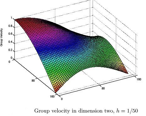
37 SPURIOUS NUMERICAL SOLUTION ϕ = exp ( ) i λ N (h) t w N exp ( ) i λ N 1 (h) t w N 1. Spurious semi-discrete wave combining the last two eigenfrequencies with very little gap: λ N (h) λ N 1 (h) h. Note that the gap is roughly the derivative of the dispersion curve. Thus this derivative determines the velocity of propagation of wave packets, the co called group velocity.

38 h = 1/61, (N = 60), 0 t 120. The solution exhibits a timeperiodicity property with period τ of the order of τ 50 which contradicts the time-periodicity of period 2 of the wave equation. High frequency wave packets travel at a group velocity h.

39

40 GAP = GROUP VELOCITY = VELOCITY OF PROPAGATION OF HIGH FREQUENCY WAVE PACKETS.

41 CONCLUSION The minima of J h diverge because its coercivity is vanishing as h 0; This is intimately related to the blow-up of the discrete observability constant C h (T ), for all T > 0 as h 0: E h (0) C h (T ) T 0 ϕ N (t) h 2 dt This is due to the lack of propagation of high frequency numerical waves due to the dispersion that the numerical grid produces.

42 Actually it is known that C h (T ) diverges exponentially: Sorin Micu, Uniform boundary controllability of a semi-discrete 1-D wave equation, Numer. Math., 91 (2002), pp In fact, by making combinations of an increasing finite number of high frequencies with nearby velocities of propagation one can build wave packets for which the observability constant blows-up polynomially at any rate. The construction by S. Micu is finer since it is based on explicit estimates on biorthogonal families to the families of complex exponentials entering in the Fourier expansion of solutions.

43 WHAT ARE THE CONSEQUENCES FOR CONTROL? Apply Banach-Steinhauss Theorem: Even when T > 2 (good control situation) there are intial data for the wave equation so that the controls of the semi-discrete problem diverge to infinity as h 0. THUS, CONTROLLING THE SEMI-DISCRETE SYSTEM IS NOT AN EFFICIENT WAY OF COMPUTING THE CONTROL OF THE WAVE EQUATION. CONTROL+NUMERICS NUMERICS+CONTROL

44 If the control requirement is sufficiently relaxed, this lack of commutativity does not occur. * Optimal control: min 1 2 * Approximate control: [ y(t ) 2 L 2 (0,1) + y t(t ) 2 ] 1 H 1 (0,1) + 2 T y(t ) L 2 (0,1) + y t((t ) H 1 (0,1) α. 0 v2 (t)dt. E. Z. Optimal and approximate control of finite-diffference schemes for the 1 D wave equation. Rendiconti di Matematica, Serie VIII, Vol. 24, Tomo II, 2004, Thi is also closely related to the technique based on the use of Tycchonoff regularization.

45 Then the controls of the discrete approximated models converge to the control of the continuous one. This can be seen by classical arguments in Numerical Analysis and in the context of Γ-convergence in the Calculus of Variations. This requires however a fine devlopment of numericalo analysis, allowing to deal, by transposition, with non-homogeneous boundary value problems, for instance.

46 What to do in practice? No general receipt. It depends on the application we have in mind. One has to make two choices: * Continuous modelling / Discrete modelling. * What control property?

47 2.3 Nonharmonic Fourier series and remedies to the divergence of controls. WHAT IS THE REMEDY? To filter the high frequencies, i.e. keep only the components of the solution corresponding to indexes: k δ/h with 0 < δ < 1.

48 Filtering restablishes the gap condition, then waves propagate with a speed which is uniform with respect to h and the observability inequality becomes uniform too. λ h ( k λ h πδ k 1 π cos 2 ) > 0, for k δh 1. This can be done rigorously with the aid of:

49 Ingham s Theorem. (1936) Let {µ k } k Z be a sequence of real numbers such that µ k+1 µ k γ > 0, k Z. Then, for any T > 2π/γ there exists C(T, γ) > 0 such that 1 C(T, γ) k Z a k 2 T 0 k Z a k e iµ kt for all sequences of complex numbers {a k } l 2. 2 dt C(T, γ) k Z a k 2

50 CONCLUSION. Given any T > 2, choose 0 < δ < 1 such that ( ) πδ T > 2/ cos or δ > 2 arccos(2/t ). 2 π The choice of 0 < δ < 1 is obviously possible since 2/T < 1. Then, we can control UNIFORMLY ON h the solution PARTIALLY: and π δ/h (y(t ), y t (T )) = 0

51 In the limit the whole solution vanishes: y(t ) = y t (T ) = 0. This is due to the fact the projection operator π δ/h tends to the identity as h 0.

52 Plot of the initial datum to be controlled for the string occupying the space interval 0 < x < 1. Plot of the time evolution of the exact control for the wave equation in time T = 4.

53 Without filtering, the control diverges as h 0.

54 With appropriate filtering the control converges as h 0.

55 These filtered controls can be computed by minimizing the functional J h leading to the controls in the subspace of filtered solutions of the adjoint system. The filtering guarantees the uniform observability. Accordingly the functionals J h are uniformly coercive over those subspaces. In this way, the functionals J h, when restricted to these classes of filtered solutions, Γ-converge to the functional J associated to the control of the wave equation. This is so, since, the filtering condition k δ/h

56 when h 0, ends up covering the whole range of frequencies. Obviously, when minimizing J h over the class of filtered solutions, we only recover partial information on the projections of the controlled states. Indeed, in the Euler-Lagrange equations associated to the minimizers, we do not recover any information on the frequencies that have been cut-off.

57 2.4 The two-grid algorithm in 1-d ULTIMATE GOAL: To develop a class of numerical schemes (new or not) for which the convergence of controls might be guaranteed a priori with minimal computational cost. The most natural approaches (finite differences and FINITE ELE- MENTS) do not work and they have to be complemented with other strategies: * filtering of high frequencies, * mixed finite elements, * multi-grid algorithms, * wavelets, * numerical viscosity,...

58 MIXED FINITE ELEMENTS Square roots of the eigenvalues both in the continuous and in the discrete case with mixed finite elements. The gap of the discrete problem is uniform with respect to j and h and, in fact, it tends to infinity for the highest frequencies as h 0.

59 The MFE can be obtained writing the wave equation as a system of two first oprder transport equations with unknowns ϕ and ϕ t. Taking into account that the regularity of ϕ is H 1 and that of ϕ t is L 2, it is natural to consider two different bases for approximating each component. Namely, P 1 pieciwise linear and continuous elements for ϕ and P 0 piecewise constant elements for ϕ t. In this way the scheme we get, when written in finite difference notation, reads, 1 4 ϕ j ϕ j ϕ j+1 = 1 [ ] ϕj 1 h 2 2ϕ j + ϕ j+1. The dispersion diagram corresponding to this scheme is as above. It is an interesting open problem to analyze the dispersion properties of the various possible MFE in the multi-dimensional case.

60 TWO-GRID ALGORITHM (R. Glowinski, M. Asch-G. Lebeau, M. Negreanu,...) High frequencies producing lack of gap and spurious numerical solutions correspond to large eigenvalues λ h N 2/h. When considering a coarser mesh h ah, λ ah N/2 1/h. Embedding data of a coarse grid 2h into the computational one of size h produces the same effect as filtering with parameter 1/2.

61 All solutions on the coarse mesh when projected to the fine one are no longer pathological. TWO GRIDS FILTERING WITH PARAMETER δ = 1/2.

62 The multiplier method allows analyzing the two-grid method easily: The multiplier xϕ x for the wave equation yields: 1 T E(0) + xϕ xϕ t dx T 0 0 = 1 2 and this implies, as needed, T 0 ϕ x(1, t) 2 dt. (T 2)E(0) 1 2 ϕ x(1, t) 2 dt. 0 The multiplier j(ϕ j+1 ϕ j 1 ) for the discrete wave equation gives: T E h (0) + X h (t) T 0 = 1 2 T 0 ϕ N (t) h T 2 dt+ h 2 N j=0 T 0 ϕ j ϕ j+1 2 dt,

63 Note that h 2 N j=0 T 0 ϕ j ϕ j+1 2 dt h2 2 T ϕ xt 2 dxdt. Filtering is needed to absorb this higher order term: For 1 j δn h 2 with 0 < γ(δ) < 1. N j=0 T 0 ϕ j ϕ j+1 2 dt γ(δ)t E(0), In this way one may recover the same results as above in an alternate way, without using Ingham s inequality and Fourier series.

64 Solutions on the fine grid of size h corresponding to slowly oscillating data given in the coarse mesh (2h) are no longer pathological: ϕ = ϕ l + ϕ h, ϕ l = (N 1)/2 k=1 c k w k, ϕ h = (N 1)/2 k=1 c k λ k λ N+1 k w N+1 k, ϕ h ϕ l.

65 This allows estimating the reminder term in the discrete multiplier identity and obtain the observability inequality. The two-grid filtering is easier to implement than the Fourier one since it can be fully implemented in the physical space.

66 Proofs: 1 d M. Negreanu & E. Z., The two-grid algorithm converges for control times T > 4. Multipliers techniques. M. Mehrenberger & P. Loreti, Same result for T > 2 2 using new versions of Ingham inequalities. M. NEGREANU & E. Z. Convergence of a multigrid method for the controllability of a 1-d wave equation. C. R. Acad. Sci. Paris, 338 (4) (2004),

67 SUMMARY: The most natural numerical methods for computing the controls diverge. Filtering of the high frequencies is needed. This may be done on the Fourier series expansion or on the physical space by a two-grid algorithm. Convergence of the controls is guaranteed by minimizing the discrete functional J h over the class of slowly oscillating data. This produces a relaxation of the control requirement: only the projection of the discrete state over the coarse mesh vanishes.

68 2.5 Links with the dynamical properties of bicharacteristic rays. In several space dimensions, the region in which the observation/control applies needs to be large enough to capture all rays of Geometric Optics. This is the so-called Geometric Control Condition introduced by Ralston (1982) and Bardos-Lebeau-Rauch (1992). Let Ω be a bounded domain of R n, n 1, with boundary Γ of class C 2. Let Γ 0 be an open and non-empty subset of Γ and T > 0. y tt y = 0 in Q = Ω (0, T ) y =v(x, t)1 Γ0 on Σ = Γ (0, T ) (x, 0) = y 0 (x), y t (x, 0) = y 1 (x) in Ω.

69 In all cases the control is equivalent to an observation problem for the adjoint wave equation: Is it true that: ϕ tt ϕ = 0 in Q = Ω (0, T ) ϕ = 0 on Σ = Γ (0, T ) ϕ(x, 0) = ϕ 0 (x), ϕ t (x, 0) = ϕ 1 (x) in Ω. E 0 C(Γ 0, T ) T 0 Γ 0 ϕ 2 dσdt? n And a sharp discussion of this inequality requires of Microlocal analysis. Partial results may be obtained by means of multipliers: x ϕ, ϕ t, ϕ,...

70 THE 5-POINT FINITE-DIFFERENCE SCHEME ϕ j,k 1 h 2 [ ϕj+1,k + ϕ j 1,k 4ϕ j,k + ϕ j,k+1 + ϕ j,k 1 ] = 0. The energy of solutions is constant in time: E h (t) = h2 2 + N N j=0 k=0 [ ϕ jk (t) 2 ϕ j+1,k (t) ϕ j,k (t) h 2 + ϕ j,k+1 (t) ϕ j,k (t) h 2. Without filtering observability inequalities fail in this case too.

71 Understanding how filtering should be used requires of a microlocal analysis of the propagation of numerical waves combining von Neumann analysis and Wigner measures developments (N. Trefethen, P. Gérard, P. L. Lions & Th. Paul, G. Lebeau, F. Macià,...). The von Neumann analysis. Symbol of the semi-discrete system for solutions of wavelength h p h (ξ, τ) = τ 2 4 ( sin 2 (ξ 1 /2) + sin 2 (ξ 2 /2) ), versus p(ξ, τ) = τ 2 [ ξ ξ 2 2 ]. Compare with the symbol of the continuous wave equation: p(ξ, τ) = τ 2 [ ξ ξ 2 2 ].

72 Both symbols coincide for (ξ 1, ξ 2 ) (0, 0). The bicharacteristic rays for the semi-discrete system are as follows: x j (s) = 2sin(ξ j/2)cos(ξ j /2) = sin(ξ j ), j = 1, 2 t (s) = τ ξ j (s) = 0, j = 1, 2 τ (s) = 0. The projection into the physical space is: x j (t) = sin(ξ j) t + x j,0. τ Solving the bicharacteristic flow we get the discrete rays: x j (t) = sin(ξ j) t + x j,0, τ (versus x j (t) = ξ j τ t + x j,0.)

73 BOTH ARE STRAIGHT LINES. BUT! For the continous wave equation all rays propagate with velocity identically equation one. Indeed, the velocity of propagation of the ray is independent of direction: Indeed, [ ξ 1 τ 2 + ξ 2 τ x j (t) = ξ j τ t + x j,0, x (t) 1. 2 ] 1/2 = 1 τ 2 ξ 2 = 0 p(ξ, τ) = 0.

74 This is equivalent to the fact that (τ, ξ) lies in the characteristic manifold. But for the semi-discrete system the velocity is x (t) sin(ξ 1 ) τ 2 + sin(ξ 2 ) τ 2 1/2 in the fol- THE VELOCITY OF PROPAGATION VANISHES!!!!!!! lowing eight points ξ 1 = 0, ±π, ξ 2 = 0, ±π, (ξ 1, ξ 2 ) (0, 0). Therefore, in order to guarantee a uniform velolicity of propagation of waves of wavelength h one has to filter or cut-off all the Fourier components on neighborhoods of those critical points.

75 The red areas stand for those that need to be filtered out in order to guarantee a uniform velocity of propagation in the semi-discrete models.

76

77 Once this is done, one guarantees a uniform velocity of propagation of numerical waves but, in order to achieve observability or controllability properties one still needs to impose a Geometric Control Condition. As filtering becomes stronger, the time of control of the numerical scheme will get closer and closer to that of the continuous wave equation. Once this is understood the 1-d results can be extended. One can then prove that, under filtering, for a suitable choice of the time interval, numerical controls converge to the real control!

78 Filtering can be performed by cutting-off the Fourier expansion of solutions. But the two-grid algorithm provides an alternate way of doing this within the physical space.

79 2.6 The two-grid algorithm in the multi-dimensional case. L. Ignat & E. Z., 2006 Theorem 1 Let Ω be the square and consider controls on all its boundary or on two consecutive sides. Then, the two-grid algorithm with mesh-ratio 1/4 converges for T sufficiently large. The proof uses: Previous results on the control of the solutions under Fourier filtering (E. Z. JMPA, 99 )

80 Fourier analysis showing that the total energy of the slowly oscillating discrete functions can be bounded above in terms of the low frequency components. A diadic decomposition argument following the level sets of the discrete symbol.

81 Grids: h & 4h

82 Low frequency subset concentrating the energy of solutions.

83 Why not using ratio 1/2 for the two-grids? The relevant zone of frequencies intersects a level set of the phase velocity for which the group velocity vanishes at some critical points.

84 CONCLUSIONS: CONTROL AND NUMERICS DO NOT COMMUTE FOURIER FILTERING, MULTI-GRID METHODS ARE GOOD REMEDIES IN SIMPLE SITUATIONS: CONSTANT COEFFI- CIENTS, REGULAR MESHES. MUCH REMAINS TO BE DONE TO HAVE A COMPLETE THEORY AND TO HANDLE MORE COMPLEX SYSTEMS. BUT ALL THE PATHOLOGIES WE HAVE DESCRIBED WILL NECESSARILY ARISE IN THOSE SITUATIONS TOO.

85 THE MATHEMATICAL THEORY NEEDS TO COMBINE TOOLS FROM PARTIAL DIFFERENTIAL EQUATIONS, CONTROL THE- ORY, CLASSICAL NUMERICAL ANALYSIS AND MICROLO- CAL ANALYSIS. OPEN PROBLEMS Complex geometries, variable and irregular coefficients, irregular meshes, the system of elasticity, nonlinear state equations,...

86

87 2.7 Links with waves in heterogenous media WELL KNOWN PHENOMENA FOR WAVES IN HIGHLY OSCILLA- TORY MEDIA

88 ϕ tt (α(x)ϕ x ) x = 0. The observability constant blows-up in the context of homogenization α = α(x/ε) as ε 0; Note the analogy between the homogenization and the discrete models: A h A ε ϕ tt + A h ϕ = 0 ϕ tt + A ε ϕ = 0 Observability fails for some coefficients α in C 0,α (BV is a sharp assumption). This also excludes Strichartz-like dispersive estimates (F. Colombini, S. Spagnolo (1989),...).

89 Pathologies are due to the existence of eigenfunctions which are highly concentrated inside the domain, with an exponentially small queu over the boundary: ϕ = e i λt w(x). F. Colombini & S. Spagnolo, Ann. Sci. ENS, 1989 M. Avellaneda, C. Bardos & J. Rauch, Asymptotic Analysis, C. Castro & E. Z. Archive Rational Mechanics and Analysis, 2002 & C. CASTRO & E. Z. Concentration and lack of observability of waves in highly heterogeneous media. Archive Rational Mechanics and Analysis, 164 (1) (2002), 39-72, & Addendum ARMA; 2006.

90 Obtaining sharp regularity estimates for coeffficients in the multidimensional case is a widely open subject. It is closely related to the topic of Strichartz inequalities. In fact the pathological examples for the lack of observability are such that there exist families of highly concentrated eigenfunctions that provide also counterexamples to dispersion.

91 2.8 Stabilization The same tools that have been developed to prove observability inequalities for wave equations (Fourier series, multipliers, Carleman inequalities, microlocal Analysis) can be applied to deal with the problem of stabilization: To produce the uniform exponential decay property in time by means of feedback (closed-loop controllers) mechanisms that are localized in the same subsets where controls are applied. Boundary stabilization of the wave equation Let Ω be a bounded domain of R n, n 1, with boundary Γ of class

92 C 2 and Γ 0 be an open and non-empty subset of Γ. y tt y = 0 in Q = Ω (0, ) y = 0 on Σ 1 = (Γ \ Γ 0 ) (0, ) y ν = y t on Σ 0 = Γ 0 (0, ) y(x, 0) = y 0 (x), y t (x, 0) = y 1 (x) in Ω. The energy is then of the form E(t) = 1 ] [ y t 2 + y 2 dx 2 Ω and satisfies the energy dissipation law de(t) dt = Γ 0 y t 2 dγ.

93 Internal stabilization. Let ω be an open subset of Ω. Consider: y tt y = y t 1 ω in Q = Ω (0, ) y = 0 on Σ = Γ (0, ) y(x, 0) = y 0 (x), y t (x, 0) = y 1 (x) in Ω, where 1 ω stands for the characteristic function of the subset ω. The energy dissipation law is then de(t) dt = ω y t 2 dx. Question: Do they exist C > 0 and γ > 0 such that E(t) Ce γt E(0), t 0, for all solution of the dissipative system?

94 The answer to the problem is roughly the same as for observability and control. Stabilization holds iff the GCC is satisfied. What about numerical schemes? The same pathologies we have described at the level of observability and control arise in this context too and are an obstacle for the decay rate to be uniform on the mesh-size parameter h.

95 Numerical viscosity L. R. Tcheugoue-Tebou, E. Z., Consider the viscous numerical approximation scheme: y j 1 h 2 [ yj+1 + y j 1 2y j ] [ y j+1 + y j 1 2y j] + aj 1 ωh y j = 0. This is the semi-discrete analog of y tt y h 2 y t + a(x)1 ω y t = 0. L. R. TCHEUGOUE & E. Z. Uniform exponential long time decay for the space semi-discretizations of a damped wave equation with artificial numerical viscosity. Numerische Mathematik, 95 (3) (2003), & Uniform boundary stabilization of the finite difference space discretization of the 1 d wave equation. Advances in Computational Mathematics, to appear.

96 The energy dissipation law is this time: de h (t) dt = h j ω h a j y j 2 h 3 N j=0 y j+1 y j 2 h 2. The right hand side terms reproduce the effect of the two damping terms in this scheme: The velocity damping, discrete version of a(x)y t ; The added viscous damping that efficiently dissipates the high frequency spurious oscillations.

97 Theorem: THE DECAY RATE OF THIS VISCOUS NUMERICAL SCHEME IS UNIFORMLY, INDEPENDENT OF h. Furthermore, the scheme converges in the classical sense of numerical analysis. Note that this result is optimal in what concerns the amount of viscous damping we use. The same exponential decay rate could be proved by using a viscous term of the form h α y t, with α < 2, but then the order of convergence of the numerical scheme would be smaller (= (h α ). On the other hand, the decay rate would fail to be uniform is less damping were used, i. e. for viscous damping terms of the form h α y t, with α > 2. This result has been later extended in various ways:

98 The 1 d wave equation with boundary damping (L. R. Tcheugoue- Tebou, E. Z. 2003); Multi-dimensional problems (A. Munch-A. Pazoto. ESAIM:COCV, to appear.) More general 1 d problems (with stronger numerical viscosity), M. Tucsnak et al., But a complete theory is to be developed.

99 2.9 Semilinear wave equations One of the most systematic approaches to derive exact controllability results for semilinear PDE consists in combining: A fixed point method; Sharp results on the cost of controlling linear equations perturbed by lower order potentials. In this way it has been proved that the semilinear 1 d wave equation y tt y xx + f(y) = 0 E. Z. Exact controllability for the semilinear wave equation in one space dimension. Ann. IHP. Analyse non linéaire

100 is controllable as the linear one is within the class of nonlinearities growing at infinity as f(s) slog 2 (s). This result is sharp since for nonlinearities that are asymptotically larger blow-up phenomena may occur and, due to the finite velocity of propagation, when blow-up occurs, exact controllability may not hold. What about numerical schemes? Most of the results we have developed are based on Fourier series decompositions that do not suffice to deal with semilinear problems.

101 The two-grid technique seems to be the most convenient one to do it. Consider the conservative finite-difference semi-discretization of the semilinear wave equation as follows: y j + 2y j y j+1 y j 1 h 2 + f(y j ) = 0, j = 1,..., N, 0 < t < T y 0 (t) = 0, y N+1 (t) = v(t), 0 < t < T (1) y j (0) = yj 0, y j (0) = y1 j, j = 0,..., N + 1. The semi-discrete analogue of the exact controllability final condition E. Z., Control and numerical approximation of the wave and heat equations, Proceedings of the ICM Madrid 2006, Vol. III, Invited Lectures, European Mathematical Society Publishing House, M. Sanz-Solé et al. eds., 2006, pp

102 is y j (T ) = z 0 j, y j (T ) = z1 j, j = 0,..., N + 1. (2) But, under the final requirement (2), controls diverge as h 0 even for the linear wave equation. In the two-grid algorithm, the final condition (2) is relaxed to ( ) ( Π h Y (T ) = Πh Z 0 ) (, Π h Y (T ) ) ( = Π h Z 1 ), (3) where Y (t) and Y (t) stand for the vector-valued unknowns Y (t) = ( y 0 (t),..., y N+1 (t) ), Y (t) = ( y 0 (t),..., y N+1 (t)). We shall also use the notation Y h for Y when passing to the limit to better underline the dependence on the parameter h. Π h is the

103 projection operator so that ( ( 1 Π h (G) = g 2j g 2j g 2j+2 )) j=0,..., N+1 2 1, (4) with G = (g 0, g 1,..., g N, g N+1 ). Note that the projection Π h (G) is a vector of dimension (N + 1) / 2. Thus, roughly speaking, the relaxed final requirement (3) only guarantees that half of the state of the numerical scheme is controlled. Despite this fact, the formal limit of (3) as h 0 is still the exact controllability condition on the continuous wave equation.

104 Theorem 2 Assume that the nonlinearity f : R R is such that f is globally Lipschitz. (5) Let T 0 > 0 be such that the two-grid algorithm for the control of the linear wave equation converges for all T > T 0. Then, the algorithm converges for the semilinear system too for all T > T 0. More precisely, for all ( y 0, y 1) H s (0, 1) H s 1 (0, 1) with s > 0, there exists a family of controls {v h } h>0 for the semi-discrete system (1) such that the solutions of (1) satisfy the relaxed controllability condition (3) and v h (t) v(t) in L 2 (0, T ), h 0 ( Yh, Y h) (y, yt ) in L 2( 0, T ; L 2 (0, 1) H 1 (0, 1) )

105 where y is the solution of the semilinear wave equation and v is a control such that the state y satisfies the final requirement. Whether the two-grid algorithm applies under the weaker and sharp growth logarithimic condition is an open problem. The difficulty for doing that is that the two existing proofs allowing to deal with the semilinear wave equation under the weaker growth condition are based, on a way or another, on the sidewise solvability of the wave equation, a property that the semi-discrete scheme fails to have. Here we are able to deal with globally Lipschitz nonlinearities, since, after linearization, they lead to linear equations ith uniformly bounded potentials. in this case a compactness-uniqueness argument suffices to obtain a (non explicit) uniform observability constant.

106 2.10 Schrödinger and plate equations DISPERSION MAY HELP At the continuous level it is well known that dispersion helps. It is well known (G. Lebeau) that, whenever the wave equation is controllable in some time T in some geometric configuration, then the Schrödinger equation is controllable too, but in an arbitrarily small time (infinite speed of propagation). But there are results showing that the Schrödinger and plate equations behave in fact better. Indeed, for instance, in the square, controllability may be achieved by means of controls supported in regions that

107 do not fulfill the GCC requirement (A. Haraux, S. Jaffard, N. Burq, M. Tucsnak,...) It is easy to see that the classical Gaussian beam construction showing that trapped rays are an obstacle for controllability for wave equations, does not yield a counterexample in the Schrödinger setting because of the infinite speed of propagation and the spreading of these beams in infinite time. Consider the Schrödinger or beam and plate equations: iu t = u Schrödinger; u tt = 2 u plate/beam Its semi-discrete versions read: iu t = h u; u tt = 2 h u.

108 Here h denotes the finite-difference approximation of the Laplacian. The Fourier representation reads now as follows: ϕ = N k=1 a k cos ( λ h k t) + b k λ h k sin ( λ h k t) w k h. This time ϕ = k=1 ( a k cos(k 2 π 2 t) + b ) k kπ sin(k2 π 2 t) sin(kπx) λ N (h) λ N 1 (h) =

109 = ( λ N (h) λ N 1 (h))( λ N (h) + λ N 1 (h)) h. 1 h 1. The gap being uniform, we can apply Ingham s inequality. The controllability properties are this time independent of h.

110

111 DISPERSION SUFFICES, BUT ONLY IN 1 D. IN SEVERAL SPACE DIMENSIONS GEOMETRY ENTERS AGAIN! Indeed, we can not recover the same results as for the continuous Schrödinger equation in the continuous setting. The following is an example showing that observability and controllability fail for all time for the semi-discrete Schrödinger equation in the square when the domain of control does not intersect the diagonal.

112 The eigenvector for the 5 point finite-difference scheme for the Laplacian in the square, with eigenvalue λ = 4/h 2, taking values ±1 along a diagonal, alternating sign and vanishing everywhere else in the domain. An interesting open problem: Laplacian. Unique continuation for the discrete

113 A h ϕ = λ ϕ ϕ j = 0, j ω h ϕ 0? The problem arises in a much more general context: general geometries, finite elements, heat and wave equations,... Generally speaking: What is the tool needed to analyze whether the fact that a solution of a discrete or semi-discrete system vanishes in a certain number of nodes, implies that the solution vanishes everywhere?

114 What is the discrete counterpart of Holmgren s Uniqueness Theorem or of Carleman s inequalities?