AN ALGORITHMIC INTRODUCTION TO NUMERICAL METHODS FOR PDES WITH RANDOM INPUTS DRAFT. Max Gunzburger

Transcription

1 AN ALGORITHMIC INTRODUCTION TO NUMERICAL METHODS FOR PDES WITH RANDOM INPUTS Max Gunzburger Department of Scientific Computing Florida State University with Clayton Webster John Burkardt Hans-Werner van Wyk Oak Ridge National Laboratory Florida State University Basque Center for Applied Mathematics Bibao, Spain April 29 to May 3, 2013

2 Sir, I have given you an argument I am not also obliged to provide you with an understanding Samuel Johnson A little inaccuracy sometimes saves tons of explanation Saki (Hector Hugh Munro) All models are wrong, but some models are useful Assumption has many advantages George Box Chiefly these are the same as those of theft over honest toil Bertrand Russell Computational results are believed by no one, except for the person who wrote the code Experimental results are believed by everyone, except for the person who ran the experiment Origin unknown

3 3 UNCERTAINTY QUANTIFICATION IN THE PDE SETTING

4 UNCERTAINTY IS EVERYWHERE 4 Physical, biological, social, economic, financial, etc. systems always involve uncertainties = mathematical models of these systems should account for uncertainty Uncertainties are often classified into two classes epistemic - uncertainty is due to incomplete knowledge of the system - uncertainty can be reduced by additional measurements, improvements in measuring devices, etc. aleatoric - uncertainty is intrinsic in the system - uncertainty cannot be reduced through additional measurements, improvements in measuring devices, etc.

5 5 Another way of classifying uncertainties = uncertainties due to incompleteness of available data - data are predictable but are too difficult (perhaps impossible) or costly to obtain by measurement media properties in oil reservoirs or aquifers - they are unpredictable wind gusts, rainfall amounts not all scales in the data and/or solutions can or should be resolved - it is too difficult (perhaps impossible) or costly to do so in a computational simulation turbulence, molecular vibrations - some scales may not be of interest surface roughness, hourly stock prices

6 6 Note that of course, it is well known that two experiments run under the same conditions will yield different results - data about a system obtained from experiments, even if it is thought of as being deterministic, is always subject to uncertainty from the point of view of numerical methods, there is no appreciable differences between the types or sources of uncertainty - thus, we will not worry about how uncertainties in systems arise

7 7 Uncertainty quantification Uncertainty quantification (UQ) the task of determining information about the uncertainty in the outputs of a system, given information about the uncertainty in the inputs of the system of course, a system may have additional inputs that are deterministic

8 8 We consider systems governed by partial differential equations (PDEs) Thus, uncertainty quantification is the task of determining information about the uncertainty in the solution of a PDE, given information about the uncertainty in the inputs of the PDE the solution of the partial differential equation defines the mapping from the input variables to the output variables

9 9 Often, the solution of the PDE is not the primary output of interest of more interest are quantities obtained by post-processing solutions of the PDE = outputs of interest - of course, one still has to obtain a solution of the PDE to determine the output of interest Thus, uncertainty quantification is the task of determining information about the uncertainty in an output of interest that depends on the solution of a PDE, given information about the uncertainty in the inputs of the PDE

10 10 There are several approaches towards UQ, both deterministic and probabilistic fuzzy sets and possibility theory, interval arithmetic, probabilistic approaches, evidence theory (e.g., Dempster-Shafer theory), etc. we consider probabilistic approaches to UQ thus, the uncertainty in the input of the PDE is described in terms of statistical quantities, i.e., probability density functions, expected values, variances, covariance functions, higher moments, etc. Thus, uncertainty quantification is the task of determining statistical information about the uncertainty in an output of interest that depends on the solution of a PDE, given statistical information about the uncertainty in the inputs of the PDE

11 TYPES OF INPUT NOISE 11 White noise input data vary randomly, independently from one point of the physical domain to another and from one time instant to another uncertainty is described in terms of uncorrelated random fields - the value of a uncorrelated random field η(x, t) at a point x and at a time t is sampled according to a given PDF independently from any other point and any other time examples: thermal fluctuations; surface roughness; Langevin dynamics very often, the terminology white noise is used only for uncorrelated Gaussian random fields

12 12 Colored (or correlated) noise input data vary randomly from one point of the physical domain to another and from one time instant to another according to a given (spatial/temporal) correlation structure uncertainty is described in terms of correlated random fields examples: rainfall amounts; bone densities; permeabilities within subsurface layers

13 13 Random parameters input data depend on a finite number of random parameters think of this case as knobs in an experiment each parameter may vary independently according to its own given probability density alternately, the parameters may vary according to a given joint probability density examples: homogeneous material properties (e.g., Young s modulus, Poisson ratio, speed of sound), inflow mass Spatially and/or time-dependent random fields, whether the are correlated or not, can also be described in terms of parameters however, because they are (infinite) stochastic processes, it takes an infinite number of random parameters to describe them

14 14 Ultimately, for all three cases, on a computer one can only solve problems involving a finite number of random parameters in the white noise and colored noise cases, one discretizes the noise so that the discretized noise is approximated in terms of a finite number of parameters - in the white noise case, the number of parameters directly depends on the spatial and/or temporal resolutions of the numerical scheme used to solve the PDEs - in the colored noise case, the number of parameters depends more weakly on the spatial/temporal resolutions

15 15 A realization of the random system is determined by and then choosing a specific set of input parameters using the PDE to determine the corresponding output variables thus, for us, a realization of the solution of the PDE is a solution for a specific choice for the input parameters - such a realization is the solution of a deterministic PDE problem thus, for us, a realization of a quantity of interest (QoI) is the QoI determined from a realization of the solution of the PDE One is never interested in individual realizations of the QoI one is interested in determining statistical information about the QoI, given statistical information about the inputs of the PDE

16 16 Input variables could be distributed independently or jointly without proper justification and sometimes incorrectly, it is almost always assumed that the parameters are independent based on empirical evidence, sometimes this is a justifiable assumption in the parameters-are- knobs case but for correlated random fields, it is justifiable only for the Gaussian case in general, independence is a simplifying assumption that is invoked for the sake of convenience, e.g., because of a lack of knowledge

17 17 Independent vs. uncorrelated Suppose we have N random parameters {y n } N n=1 defined over an N-dimensional set Γ a joint probability density function (PDF) ρ(y 1,..., y N ) is a mapping from Γ into the real numbers such that and ρ(y 1,..., y N ) 0 for all {y 1,..., y N } Γ Γ ρ(y 1,..., y N ) dy 1 dy N = 1

18 18 For n = 1,..., N, the mean or expected value of y n is given by µ n = E(y n ) = if µ n = 0, then y n is called centered Γ y n ρ(y 1,..., y N ) dy 1 dy N The covariance of {y n } N n=1 is the N N matrix C given by C nn ( ) = E (y n µ n )(y n µ n ) = Γ (y n µ n )(y n µ n )ρ(y 1,..., y N ) dy 1 dy N = E(y n y n ) E(y n )E(y n ) = E(y n y n ) µ n µ n if either y n or y n is centered C nn = E(y n y n )

19 19 The random variables {y n } N n=1 are independent if the choice of values of any subset of parameters does not depend on the choices made for the values of the remaining parameters the random variables {y n } N n=1 are independent if and only if the joint PDF is a product of the PDFs for the individual parameters N ρ(y 1,..., y N ) = ρ n (y n ) where, for each n = 1,..., N, ρ n ( ) is a mapping from an interval Γ n to the real numbers that satisfies ρ n (y n ) 0 ρ n (y n ) dy n = 1 Γ n note that then Γ is the hyper-rectangle Γ = Γ 1 Γ 2 Γ N n=1 note that the intervals Γ n maybe of finite (e.g., for a uniform distribution) or infinite (e.g., for a Gaussian distribution) extent

20 20 The random variables {y n } N n=1 are uncorrelated only if C nn = σ 2 nδ nn = { 1 if n = n where σn 2 denotes the variance of y n ) σn 2 = C nn = E ((y n µ n ) 2 = Γ 0 if n n n, n = 1,..., N (y n µ n ) 2 ρ(y 1,..., y N ) dy 1 dy N = E(y 2 n) µ 2 n if y n is centered σ 2 n = C nn = E(y 2 n)

21 21 Independence implies uncorrelated if n n, then C nn = (y n µ n )(y n µ n )ρ(y 1,..., y N ) dy 1 dy N = = = Γ Γ 1 Γ 2 Γ N (y n µ n )(y n µ n ) Γ n (y n µ n )ρ n (y n ) dy n Γ n N ρ n (y n ) dy 1 dy N n=1 (y n µ n )ρ n (y n ) dy n N n =1, n n, n n Γ n (y n µ n )ρ n (y n ) dy n Γ n = E(y n µ n )E(y n µ n ) = 0 Γ n ρ n (y n ) dy n (y n µ n )ρ n (y n ) dy n

22 22 However, uncorrelated does not necessarily imply independence let y 1 be uniformly distributed on [ 1, 1] = E(y 1 ) = 0 E(y1) 3 = 0 let y 2 = 3 2 y2 1 clearly, {y 1, y 2 } is not independent however, {y 1, y 2 } is uncorrelated C 12 = C 21 = E(y 1 y 2 ) E(y 1 )E(y 2 ) = 3 2 E(y3 1) = 0 When does uncorrelated imply independence? if and only if the variables follow a multivariate Gaussian distribution

23 OUTPUTS 23 We assume that we are given a random input parameterized using the random parameters {y 1, y 2,..., y N } we use the abbreviation y = {y 1, y 2,..., y N } these parameters can be actual parameters appearing in the specification of the PDE, or could arise from approximations of random field inputs The solution of the PDE is not only a function of the spatial variable x and perhaps also time t, it also a function of the random parameters y Realization = a solution u(x, t; y) of a PDE for a specific choice y = {y n } N n=1 for the random parameters as mentioned before, there is no interest in individual realizations

24 24 What then are the outputs of interest? statistical information - expected values, variances, standard deviations, higher moments, PDFs statistical information about what? - usually not about the solution of the PDE at points x and times t instead, one is interested in statistical information about quantities derived from the solution of the PDE it is now common to refer to statistical information about such quantities as quantities of interest (QoIs)

25 INVERSE PROBLEMS 25 We have tacitly assumed, as is often done, that we know the PDFs of the input parameters Actually, in practice, one usually does not know much about the statistics of the input variables one is lucky if one knows a range of values, e.g., maximum and minimum values, for an input parameter - in which case one often assumes that the parameter is uniformly distributed over that range if one is luckier, one knows the mean and variance for the input parameter - in which case one often assumes that the parameter is normally distributed of course, one may be completely wrong in assuming such simple probability distributions for a parameter

26 26 2 PDFs with the same mean and variance This leads to the need to solve stochastic model calibration problems

27 27 Model calibration Model calibration is the task of determining statistical information about the inputs of a system, given statistical information about the outputs e.g., one can use experimental or field observations to determine the statistical information about the outputs in particular, one would like to identify the probability density functions (PDF) of the input variables Of course, the system still maps the inputs to the outputs thus, determining the input PDF is an inverse problem usually involves an iteration in which guesses for the input PDF are updated several ways to do the update, e.g., Bayesean,...

28 28 Uncertainty quantification direct problem Model calibration inverse problem

29 29 Model calibration problems are a particular case of more general stochastic inverse, or parameter identification, or control, or optimization problems Feedback control Optimal control

30 30 THE CURSE OF DIMENSIONALITY In almost all cases, i.e., for almost all methods, the computational costs associated with uncertainty quantification of systems governed by PDEs increases with the number of parameters used to model the uncertainty Of course, this is something we are used to after all, we are all used to having problems in three spatial dimensions costing more to solve than those in two and one dimension What we are not used to is that the number of random parameters N can be much bigger than 2 or 3

31 As a result, many numerical methods we are familiar with and perhaps have used for spatial discretization, e.g., for quadrature, become too costly to use in fact, almost of all of them become unviable even for a moderate number of parameters This is because the costs increase very, very quickly the phrase the curse of dimensionality is ubiquitously used to describe this phenomenum In one way or another, all work on UQ for systems governed by PDEs is directed at alleviating the curse the curse cannot be completely removed all one can try to do is to increase the value of N at which the curse stops us - to increase the value of N at which our computer resources become exhausted 31

32 32 QUANTITIES OF INTEREST

33 33 QUANTITIES OF INTEREST (QoIs) Determining statistical quantities of interest requires integration over the parameter domain Γ Statistical QoIs are determined as follows: from the solution u(x, t; y) of the PDE, define an output of interest F (u) choose what statistical information about F (u) is desired use the choice made for the output of interest and the choice made for the desired statistical information to define an integrand G(u) the QoI is obtained by integrating G(u), multiplied by the input PDF, over the parameter domain Γ

34 34 For example, suppose the output of interest is F (u) = u, the magnitude of the spatial gradient of the solution u of the PDE suppose the statistical information one wants is the second moment then G(u) = (F (u)) 2 = u 2 - the power of 2 comes from the second moment choice suppose ρ( y) denotes the PDF of the input parameters then, the QoI is given by QoI(x, t) = Γ G(u)ρ( y) d y = Γ u 2 ρ( y) d y note that the QoI is an integral over the parameter domain Γ note that this particular QoI is a function of x and t

35 35 We ll work backwards to discuss QoIs in more generality QoIs are defined in terms of the parameter integral QoI = Γ G ( u(x, t; y); x, t, y ) ρ( y) d y the integrand G ( u(x, t; y); x, t, y ) depends on the solution u(x, t; y) of the PDE and perhaps also depends explicitly on the physical variables x and t and the parameters y

36 36 The functional form of G ( u(x, t; y); x, t, y ) is determined from an output of interest F ( u(x, t; y); x, t, y ) and the particular statistical information one seeks about that quantity in the latter regard, if the statistical information is, for example, - the expected value of F = G = F - the m th moment of F = G = F m - the variance of F = G = ( F E(F ) ) 2 - etc. Lastly, we have to discuss some possibilities for how the output of interest F ( u(x, t; y); x, t, y ) is determined from the solution u(x, t; y) of the PDE

37 37 Outputs of interest The output of interest F ( u(x, t; y); x, t, y ) could be directly related to the solution u of the PDE e.g., F = u, F = u 2, F = u, F = u 2, F = u/ t,... this type of F arises, for example, in determining QoIs such as - the average or expected value of the solution u of the PDE u(x, t) = E[u(x, t; y)] = u(x, t; y)ρ( y) d y for which we have F = u and G = F = u - the second moment of the solution u of the PDE M 2 (x, t) = E [( u(x, t; y) ) 2] ( ) 2ρ( y) = u(x, t; y) d y for which we have F = u and G = F 2 = u 2 Γ Γ

38 - the variance of the solution u of the PDE var(x, t) = E [( u(x, t; y) u(x, t) ) 2] ( ) 2ρ( y) = u(x, t; y) u(x, t) d y Γ = M 2 (x, t) ( u(x, t) ) 2 for which we have F = u and G = ( F E(F ) ) 2 = ( u E(u) ) 2 - etc. one may define similar QoIs by substituting any quantity directly depending on u (e.g., u 2, u 3, u, u, e u, etc.) wherever u appears in the above expressions - e.g., we could be interested in the third statistical moment of e u, in which case we have the QoI QoI(x, t) = e 3u(x,t; y) ρ( y) d y for which we have F = e u and G = F 3 = (e u ) 3 = e 3u Γ 38

39 note that the same QoI can be arrived at through different pairs of choices for the output of interest F and the statistical information one wants about F 39 - for example, the third moment of u 2 (F = u 2 and G = (u 2 ) 3 = u 6 ) and the sixth moment of u (F = u and G = u 6 ) obviously lead to the same QoI From the above examples, we see that if the output of interest F ( u; x, t, y ) is directly related to the solution u of the PDE, we have that QoI = QoI(x, t)), i.e., we have a pointwise-defined QoI such pointwise QoIs, i.e., those defined at points x and time instants t, are not the ones of most interest in practice

40 40 Of greater interest are QoIs involving outputs of interest F that are spatial and/or temporal integrals of a quantity H ( u(x, t, y); x, t, y ) that depends on the solution u of the PDE let D denote a spatial domain with boundary D and (t 0, t 1 ) denote a time interval suppose that the quantity H ( u(x, t, y); x, t, y ) is derived from the solution u(x, t, y) of the PDE - e.g., H = u, H = u 4, H = u 2, H = u/ t, H = e u,... suppose that the output of interest is the spatial/temporal average of H so that t1 F ( y) = H ( u(x, t, y); x, t, y ) dxdt t 0 D suppose that the statistical information that we want about F is its expected value so that G( y) = F ( y)

41 41 we then have the QoI QoI = E[G( y)] = G( y)ρ( y) d y = F ( y)ρ( y) d y Γ Γ t1 = H ( u(x, t, y); x, t, y ) ρ( y) dxdtd y Γ t 0 D i.e., the statistical expected value (or mean) of the spatial/temporal average of H if instead, we are interested in the second moment of the the spatial/temporal average of H, we would have G( y) = ( F ( y) ) 2 and the QoI ( ) 2ρ( y) QoI = E[G( y)] = G( y)ρ( y) d y = F ( y) d y Γ Γ ( t 1 = H ( u(x, t, y); x, t, y ) 2ρ( y)d y dxdt) Γ t 0 D note that these two QoIs are just numbers, i.e., they are not functions of x, t, or y

42 42 there are many other possible outputs of interest F that involve spatial and/or temporal integrals of H, including, for example F (t; y) = F (x; y) = F (t; y) = F (t; y) = D t1 t 0 D D H(u; x, t, y) dx H(u; x, t, y) dt H(u; x, t, y) dx H(u; x, t, y) dx and many other possibilities - spatial average of H - F and G are functions of t and y - the QoI is a function of t - temporal average of H - F and G are functions of x and y - the QoI is a function of x - average of H over boundary of D - F and G are functions of t and y - the QoI is a function of t - average of H over subset D D - F and G are functions of t and y - the QoI is a function of t

43 as an example of a QoI involving spatial and/or temporal integrals, consider the second moment of the space-time average of the solution u of the PDE for which 43 - H(u; x, t, y) = u t1 - F ( y) = u(x, t; y) dx dt t 0 D - G( y) = ( F ( y) ) 2 - QoI = Γ ( t 1 t 0 D u(x, t; y) dxdt) 2ρ( y)d y

44 44 as another example, suppose u(x, t; y) denotes a flow velocity field and a denotes half the fluid density which we assume is constant and deterministic; then, consider the expected value of the total kinetic energy in the domain D at time t for which - H(u; x, t, y) = au u - F (t; y) = a u(x, t; y) u(x, t; y) dx D - G( y) = F ( y) ( - QoI(t) = a Γ D ) u(x, t; y) u(x, t; y) dx ρ( y)d y

45 A class of important outputs of interest that do not involve spatial or temporal integrals is defined as follows 45 we again have a quantity H ( u(x, t, y); x, t, y ) that depends on the solution u of the PDE we now have that the output of interest is the maximum value of H over the spatial domain D and the time interval (t 0, t 1 ) so that F ( y) = max x D, t (t 0,t 1 ) H(u; x, t, y) suppose that the statistical information that we want about F is its expected value so that G( y) = F ( y) we then have the QoI QoI = E[G( y)] = G( y)ρ( y) d y = F ( y)ρ( y) d y Γ Γ ( = max H( u(x, t, y); x, t, y )) ρ( y)d y Γ x D, t (t 0,t 1 ) i.e., the statistical expected value (or mean) of the maximum value of H over the spatial domain D and time interval (t 0, t 1 )

46 46 if instead, we are interested in the second moment of the maximum value of H over the spatial domain D and time interval (t 0, t 1 ), we would have G( y) = ( F ( y) ) 2 and the QoI QoI = E[G( y)] = ( = Γ Γ G( y)ρ( y) d y = Γ ( F ( y) ) 2ρ( y) d y max x D, t (t 0,t 1 ) H( u(x, t, y); x, t, y )) 2 ρ( y)d y of course, we have many other possible outputs of interest and QoIs of this type for example, in addition to the maximum value of H over the spatial domain D and time interval (t 0, t 1 ), we have the possibilities

47 for example, in addition to the maximum value of H over the spatial domain D and time interval (t 0, t 1 ), we have the possibilities 47 F (t; y) = max x D H(u; x, t, y) F (x; y) = max H(u; x, t, y) t (t 0,t 1 ) F (t; y) = max H(u; x, t, y) x D F (t; y) = max x D H(u; x, t, y) { F is the maximum of H over the spatial domain D { F is the maximum of H over the time interval (t 0, t 1 ) F is the maximum of H over the boundary D of the spatial domain D F is the maximum of H over the subset D of the spatial domain D and many other possibilities

48 48 as an example of a QoI of this type, let u denote the displacement vector in a solid; then, for a homogeneous, isotropic material, the stress tensor is given by T = λ( E)I + 2µE, where we have the Lame constants λ and µ and the strain tensor E = 1 2( u + ( u) T ) ; note that T = T(u); as a measure of the size of the stress, we use the Frobenius norm T ; now consider the expected value of the maximum of the Frobenius norm of the stress as the QoI; we then have that - H(u; x, t, y) = T(u) - F ( y) = max H(u; x, t, y) = max x D, t (t 0,t 1 ) - G( y) = F ( y) = max x D, t (t0,t 1 ) T ( u(x, t, y) ) - QoI = Γ ( max T( u(x, t, y) ) ) ρ( y)d y x D, t (t 0,t 1 ) T( u(x, t, y) ) x D, t (t 0,t 1 )

49 49 An extremely important class of QoIs requires the determination of the probability that a quantity derived from the solution of the PDE exceeds a given value often in this setting, the output of interest F is a functional of u, i.e., F ( u(x, t; y) ) is a (scalar-valued) number then, the problem at hand is to determine, given F 0, the QoI prob [ F ( u(x, t; y) ) F 0 ] this QoI does not seem, at first glance, to involve an integral over the parameter domain Γ, but, in fact, this QoI can also be expressed in this manner because, if χ F F0 ( y) denotes characteristic or indicator function for F F 0, i.e., { ( ) 1 if F u(x, t; y) F0 then χ F F0 ( y) = 0 otherwise QoI = prob [ F ( u(x, t; y) ) F 0 ] = Γ χ F F0 ( y)ρ( y) d y

50 thus, with G( y) = χ F F0, we again see that the QoI has the form QoI = G( y)ρ( y) d y Γ returning to the example of the stress in a solid, we note that there is usually much more interest in knowing the probability that some measure of the stress exceeds a given threshold value (e.g., a value for which a structure may fall down or crack) that in knowing statistics such as the expected value of that measure; thus, we now have, for some τ, - H(u; x, t, y) = T(u) - F ( y) = max x D, t (t 0,t 1 ) H(u; x, t, y) = max - G( y) = χ F ( y) F0 = χ maxx D, t (t0,t 1 ) T(u(x,t, y)) τ - QoI = Γ T( u(x, t, y) ) x D, t (t 0,t 1 ) χ maxx D, t (t0,t 1 ) T(u(x,t, y)) τρ( y) d y = prob[ T(u) τ ] 50

51 51 QUADRATURE RULES FOR STOCHASTIC INTEGRALS We have seen that QoIs require integration over the parameter space for some G( ), one must evaluate integrals of the type G ( u(x, t; y); x, t, y ) ρ( y) d y Γ such integrals cannot, in general, be evaluated exactly - they have to be approximated using a quadrature rule It makes a huge difference (when choosing a quadrature rule) whether or not the integrand is smooth or not in particular, discontinuous integrands as is the case if the characteristic function is involved are especially troublesome

52 Quadrature rules have the general form G ( u(x, t; y); x, t, y ) Q ρ( y) d y w q G ( ) u(x, t; y q ); x, t, y q ρ( yq ) Γ for some choice of quadrature weights {w q } Q q=1 quadrature points { y q } Q q=1 q=1 (real numbers) (points in the parameter domain Γ) alternately, sometimes the probability density function is used in the determination of the quadrature points and weights so that instead one ends up with the approximation G ( u(x, t; y); x, t, y ) Q ρ( y) d y w q G ( ) u(x, t; y q ); x, t, y q Γ q=1 in one dimension, examples of the first type of quadrature rule would be the trapezoidal and Simpson rules and their composite versions whereas examples of the second would be Gauss-Hermite or Gauss-Legendre rules and their composite versions 52

53 Monte Carlo integration the simplest rule = randomly select Q points { y q } Q q=1 in Γ 53 evaluate the integrand at each of the sample points average the values so obtained (so that, for all q, w q = 1/Q) so that, if the samples are chosen uniformly in Γ G ( u(x, t; y); x, t, y ) ρ( y) d y V (Γ) Q G ( ) u(x, t; y q ); x, t, y q ρ( yq ) Q Γ where V (Γ) denotes the volume of Γ if the sample points are instead chosen according to the PDF ρ( y), we have Q G ( ) u(x, t; y q ); x, t, y q Γ G ( u(x, t; y); x, t, y ) ρ( y) d y V (Γ) Q q=1 q=1 more on Monte Carlo and other quadrature rules later

54 54 DETERMINING PDFS So far, we have failed to consider the ideal QoI, namely, the PDF of the output of interest Outputs of interest are functions of the parameters y, but their PDFs are not the same as the PDF ρ( y) of the inputs for simplicity, we also consider the case where the output of interest is a scalar function and is a function of y but not of x or t - for example, the output of interest involves spatial and temporal integrals or involves the maximum value over the spatial-temporal domain extensions to more general cases are, at least conceptually, straightforward

55 55 Methods for determining approximate output PDFs include binning methods moment methods Bayesean methods deriving a partial differential equation for the PDF We briefly consider the first two of these

56 56 Binning methods for determining PDFs The sampling + binning method is the most popular method for determining approximate PDFs of an output of interest Suppose that the input parameters y have the joint PDF ρ( y) F ( y) denotes the output of interest Sample the PDF ρ( y) M times to produce the M parameter sets { y m } M m=1 For m = 1,..., M, evaluate the output of interest for the parameter value ym to determine the output values { F m = F ( y m )} M m=1 Determine F max = max m=1,...,m Fm and F min = min m=1,...,m Fm Set F = ( F max F min )/K and set F k = F min + k F for k = 0,..., K

57 57 Divide the interval [F min, F max ] into K equal subintervals {I k = [F k 1, F k )} K 1 k=1 and I K = [F K 1, F K ] For k = 1,..., K, set M k = the cardinality of the set { F m I k, m = 1,..., M} For k = 1,..., K, set M k = M K /M The piecewise constant function θ K,M (F ) = M k for F I k, k = 1,..., K is then an approximation of the PDF ρ F (F ) for the output of interest F

58 58 Note that this displays the PDF ρ F (F ) of F as a function of F

59 59 Determining PDFs from moments Another seemingly attractive method for computing approximations of an output PDF is to determine it from the moments of the output or interest warning: in general, PDFs are not uniquely determined by their moments - e.g., none of the moments corresponding to the PDF ρ(y) = 1 y 2π e 1 2 (ln y)2( ) 1 + a sin(2π ln y) 1 a 1 depend on a there have been many methods proposed for PDF recovery from its moments here, we consider the Gram-Charlier expansion of a PDF in terms of its moments - several generalizations and improvements of the Gram-Charlier approach have also been developed

60 60 If F is the (scalar) random output of interest and ρ F (F ) is its associated PDF, we have that the m th moment M m is defined by M m = F m ρ F (F ) df the zeroth moment is equal to 1 and the first moment is equal to the mean (expected value) of F we assume, without loss of generality, that F has zero mean and unit variance - the general case can be reduced to this case by removing the mean by subtraction and normalizing the variance by scaling Let g(f ) = 1 2π e F 2 2 denote the PDF for the standard normal distribution

61 61 Let H m (F ) denote the normalized Hermite polynomial of degree m, where by normalized we mean that H m (0) = 1 we have that H m (F )H m (F )g(f ) df = m!δ mm Then, the PDF ρ F (F ) has the expansion ρ F (F ) = c m H m (F )g(f ) = 1 2π m=0 m=0 c m H m (F )e F 2 2 where the coefficients c m, m = 1,...,, are given by c m = 1 ( M m b m2 m! 2 1! M m 2 + b m ! M m 4 b ) m ! M m 6 + where b mm = m!/(m m )!

62 62 Calculating up to first five terms, we have ρ F (F ) = ( M 3H 3 (F ) (M 4 3)H 4 (F ) + )e F 2 2 In practice, one uses truncations of the Gram-Charlier expansion to approximate ρ F (F ) the zeroth approximation is the Gaussian PDF g(f ) = e F 2 2 thus, truncated Gram-Charlier expansions yields approximations of ρ F (F ) that are corrections of the Gaussian PDF often, Gram-Charlier expansions converge slowly which is why people continuously look for improvements

63 How does one obtain the moments of an output of interest F to use in the Gram-Charlier formula? 63 The m-th moment we want is M m = F m ρ F (F ) df where ρ F (F ) is the PDF for F which we don t know (and in fact, which we are trying to find) We can estimate M m from data we do this by generating the numbers F r = F ( y r ), r = 1,..., R, where y r are sample points in Γ then the m-th moment is estimated by M m 1 R R this estimate looses accuracy as m increases so that in practice, one seldom goes beyond m = 4 r=1 F m k

64 We also have that M m = F m ρ F (F ) df = Γ ( F ( y) ) mρ( y) d y which we can approximate in the usual way using a quadrature rule to obtain Q ( M m w q F ( yq ) ) m ρ( yq ) q=1 where F ( y q ) = F ( u( y q ) ) is obtained by solving the PDE with the parameters y q 64

65 65 WHITE NOISE

66 66 WHITE NOISE FIELDS The value of a white noise random field η white (x, t; ω) at every point in space and at every instant in time is independently and identically distributed (i.i.d.) according to a Gaussian distribution the inclusion of ω in the argument of the random field indicates that the values of the random field at any point x and any time instant t are determined by - first sampling ω according to a one-dimensional PDF ρ(ω) which here is the standard normal distribution N(0, 1) - then adjusting the sample value taken for the point x and time instant t so that it would be a sample from the normal distribution having mean µ white (x, t) and variance σwhite 2 (x, t) - as a result, the sample value used = σ white (x, t)ω + µ white (x, t) - note that σwhite 2 is usually chosen to be constant

67 The covariance function corresponding to a white noise random field η white (x, t; ω) is given by Cov white (x, t, x, t ) = σ white (x, t)σ white (x, t )δ(x x )δ(t t ) where δ( ) denotes the Dirac delta function the variance V white (x) = Cov white (x, t, x, t) of white noise is infinite Obviously, in any computer simulation, one cannot sample the Gaussian distribution at every point of the spatial domain and at every instant of time white noise is replaced by discretized white noise - discretized white noise is more regular than white noise Despite the infinite variance, we can still define approximations of white noise Among the means available for discretizing white noise, grid-based methods are the most popular 67

68 68 GRID-BASED METHODS FOR DISCRETIZING WHITE NOISE For simplicity, we first consider time-independent white noise random fields To define a single realization of grid-based discretized white noise, we first subdivide the spatial domain D into N non-overlapping, covering subdomains {D n } N n=1 Then, for each n = 1,..., N, we let V n denote the volume of the subdomain D n χ n (x) denote the characteristic (or indicator) function corresponding to the subdomain D n y n (ω) denote an N(0, 1) i.i.d. random number - thus, for each k, the value of y n (ω) is independent of the value of y n(ω) for all n n

69 69 Then, for some constants {a n } N n=1 we seek an approximation of the white noise random field η white (x; ω) of the form η N white(x; ω) = µ white (x) + N a n χ n (x)y n (ω) η white (x; ω) n=1 note that this is a piecewise constant approximation (with respect to the subdivision {D n } N n=1 of the spatial domain D) of the random field η white (x; ω) µ white (x) To determine the coefficients {a n } N n=1 we first construct a piecewise constant approximation of the covariance function Cov white (x, x ) we then choose the coefficients {a n } N n=1 so that the covariance function for the approximate white noise random field ηwhite N (x; ω) is the same as the piecewise constant approximation of Cov white (x, x ) Usually the mean function µ white (x) is also approximated by a function µ N white (x) defined with respect to the grid

70 70 Specifically, we define the piecewise constant approximation of Cov white (x, x ) given by N N Cov N white(x, x ) = c ll χ l (x)χ l (x ) note that recall that l=1 l =1 Cov N white(x, x ) = c nn for x D n and x D n Cov white (x, x ) = 0 whenever x x because of its piecewise constant nature, we cannot require the same condition for Cov N white(x, x ) the best we can to is to require that then Cov N white(x, x ) = 0 whenever x D n and x D n with n n c nn = 0 for n n

71 71 we then have that Cov N white(x, x ) = N c ll χ l (x)χ l (x ) when both x and x are in D n, we can match Cov N white(x, x ), which is nonsingular, to the possibly singular Cov N white(x, x ) only in an average sense so we set so that so that D n D n Cov N white(x, x ) dx dx = N c ll l=1 = D n c nn = 1 l=1 D n Vn 2 D n χ l (x)χ l (x ) dx dx D n D n Cov white (x, x ) dx dx D n σ white (x)σ white (x )δ(x x ) dx dx D n σ 2 white(x) dx for n = 1,..., K

72 72 approximating the remaining integral by a piecewise constant approximation, we obtain c nn = 1 V n σ 2 white(x n) where x n denotes, e.g., the centroid of D n we then have that Cov N white(x, x ) = N n=1 for n = 1,..., K σwhite 2 (x n) χ n (x)χ n (x ) V n

73 The covariance matrix for the discrete random field ηwhite N (x; ω) is given by N ( N = E = = = N n=1 N n=1 n=1 n=1 a n χ n (x)y n (ω), n =1 ) a nχ n (x )y n (ω) N a n a nχ n (x)χ n (x )E ( y n (ω)y n (ω) ) n =1 N a n a nχ n (x)χ n (x )δ nn n =1 N { a a 2 nχ n (x)χ n (x 2 ) = n if both x, x D n 0 otherwise Equating with the covariance function for the piecewise constant approximation Cov N white(x, x ), we have that Vn a n = σ white(x n) 73

74 Thus, the discretized random field is given by N ηwhite(x; N ω) = µ white (x) + n=1 σ white (x n) Vn χ n (x)y n (ω) η white (x; ω) thus, via discretization, white noise has been reduced to the case of N random parameters If σ(x) = σ white = constant, as is often the case, then η N white(x; ω) = µ white (x) + σ white N n=1 1 Vn χ n (x)y n (ω) η white (x; ω) For example, in one dimension, for constant variance σwhite 2 and zero expected value and for a uniform grid of size h, we have the well-known formula η N white(x; ω) = σ white h N n=1 for approximating a white noise random field. χ n (x)y n (ω) η white (x; ω) 74

75 Note that we have constructed an approximate white noise field based on sampling in subdomains this is convenient for finite element spatial discretization schemes for other discretization schemes, e.g., finite difference spatial discretizations, it may be more convenient to sample at grid points - the construction process we have discussed is easily amended to this case What about non-gaussian white noise fields? it seems an easy matter to sample according to a different PDF instead of the normal distribution - indeed, this is done in practice however, there are serious issues that arise when doing so - not the least of which is that Gaussian PDF is the only one which is completely defined by its mean and variance 75

76 76 Grid-based approximations of time-dependent white noise fields We now consider white noise fields η white (x, t; ω) that also depend on time To define a single realization of the discretized white noise, we subdivide the spatial domain D into N space subdomains {D ns } N space n s =1 - let V ns denote the volume of D ns - let χ ns (x) denote the characteristic function for D ns subdivide the temporal interval [0, T ] into N time time subintervals {I nt } N time n t =1 - let t nt denote the length of the time interval I nt - let χ nt (t) denote the characteristic function for I nt in subdomain D ns and during the time interval I nt, let σ white (x n s, t n t ) denote a constant approximation of the given variance function σ white (x, t) let {y ns,n t } N s,n t n s =1,n t =1 denote N = N sn t i.i.d. random numbers drawn from the standard normal distribution

77 77 we then have the approximation η N space,n time white = N time n t =1 N space n s =1 σ(x, t ) tnt Vns χ nt (t)χ ns (x)y ns,n t η white (x, t; ω) - thus, via discretization, white noise has been reduced to the case of N = N s N t random parameters In the n s -th spatial subdomain having volume V ns and in the n t -th temporal subinterval having duration t nt, we have where y ns,n t variance η N space,n time white (x, t; {y ns,n t }) = 1 y ns,n t tnt Vns are independent Gaussian samples having zero mean and unit Additional realizations are defined by resampling over the space-time grid

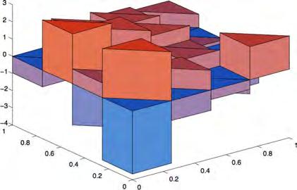
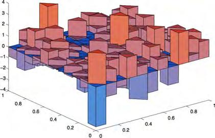
78 78 Realizations of discretized white noise at a same time interval in a square subdivided into 2, 8, 32, 72, 238, 242, 338, and 512 triangles

79 79 Realizations of discretized white noise at two different time intervals in a square subdivided into the same number of triangles Thus, the discretized white noise is piecewise constant in space and time Note that the piecewise constant function is much smoother than the random field it approximates

80 The white noise case has been reduced to a case of a large but finite number of parameters we have the N = N space N time parameters y ns,n t where n s = 1,..., N space and n t = 1,..., N time if we refine the spatial grid and/or reduce the time step, the number of parameters increases It can be shown that ) lim E( η N space,n time N space, N time white (x, t; ω)}) η N space,n time white (x, t; ω)}) = E ( η white (x, t; ω)η white (x, t; ω) ) = δ(x x )δ(t t ) 80

81 81 PDE S FORCED BY WHITE NOISE Formally, we can write an evolution equation with white noise forcing as u t = A(u; x, t) + f(x, t) + B(u; x, t)η(x, t; ω) in D (0, T ] where A is a possibly nonlinear deterministic operator f is a deterministic forcing function B is a possibly nonlinear deterministic operator η is the white noise forcing function among many other cases, A, f, and B can take care of cases with means 0 and variances 1

82 If B is independent of u, we have additive white noise 82 u t in practice, often b is a constant = A(u; x, t) + f(x, t) + b(x, t) η(x, t) If B depends on u, we have multiplicative white noise of particular interest is the case of B linear in u u t = A(u; x, t) + f(x, t) + b(x, t)u η(x, t)

83 Solutions are not sufficiently regular for the equations just written to make sense 83 the renowned Ito calculus is introduced to make sense of differential equations with white noise forcing White noise need not be restricted to forcing terms in the PDE in practice, it can also appear - in the coefficients of the PDEs and boundary and initial conditions - in the data in boundary and initial conditions - in the definition of the domain in certain cases, one must be careful about choosing coefficients, e.g., consider (η white (x; ω) u ) = f(x) - clearly, if η white (x; ω) is a Gaussian random field, then η white (x; ω) is not of one sign, in which case this problem is not well posed - more on this later

84 Spatial discretization of the PDE can be effected via a finite element method based on a triangulation of the spatial domain D; temporal discretization is effected via a finite difference method, e.g., a backward Euler method 84 it is natural to use the same grids in space and time as are used to discretize the white noise thus, if one refines the finite element grid and the time step, one also refines the grid and time step for the white noise discretization Once a realization of the discretized noise is chosen, i.e., once one chooses the N = N space N time Gaussian samples y ns,n t, a realization of the solution of the PDE is determined by solving a deterministic problem

85 For example, consider the problem u t = u + f(x, t) + b(x, t)u η(x, t; ω) in D (0, T ] subdivide [0, T ] into N time subintervals of duration t nt, n t = 1,..., N time u(x, 0) = u 0 (x) subdivide D into N space finite elements {D ns } N space n s =1 u = 0 in D (0, T ] in D define a finite element space S h 0 H 1 0(D) with respect to the grid {D ns } N space n s =1 85

86 choose an approximation u (0,h) (x) to the initial data u 0 (x) 86 sample, from a standard Gaussian distribution, the N space N time values y ns,n t, n s = 1,..., N space and n t = 1,..., N time set u (0) h (x) = u (0,h)(x) then, for n t = 1,..., N time, determine u (n t) h (x) S0 h from D = u (n t) h D u (n t 1) h v h dx + t nt fv h dx + 1 tnt u (n) h D N s v h dx n s =1 1 Vns D n s y ns,n t v h dx for all v h S h 0 - note that we have used a backward-euler time stepping scheme

87 This is a standard discrete finite element system for the heat equation, albeit with an unusual right-hand side 87 Due to the lack of regularity of solutions of PDE s with white noise, the usual notions of convergence of the approximate solution to the exact solution do not hold, even in expectation one has to be satisfied with very weak notions of convergence

88 88 Quantities of interest for white noise inputs We have our usual QoI QoI = Γ G ( u(x, t; y); x, t, y ) ρ( y) d y for some output of interest G ( u(x, t; y); x, t, y ) When an input is a discretized white noise fields, we are in a setting for which we have a huge number of random parameters we, in fact, have N = N space N time parameters, where N space is proportional to the number of grid cells and N time is proportional to the number of time steps thus, to approximate the parameter integral appearing in the QoI, we led to choosing a Monte Carlo rule - in practice, this is in fact by far the most popular choice

89 For example, we randomly select Q points { y q } Q q=1 in Γ - this means that, for each q = 1,..., Q, we select an N-vector of i.i.d. random numbers from the standard normal distribution then, for each q = 1,..., Q, we evaluate the approximate random field η N space,n time white (x, t; y q ) we then solve the (discretized) PDE for that approximate random field to obtain an approximation u approx (x, t; y q ) of the solution of the PDE finally, we obtain the approximation of the QoI given by G ( u(x, t; y); x, t, y ) ρ( y) d y 1 Q G ( ) u(x, t; y q ); x, t, y q Γ Q q=1 89

90 90 COLORED NOISE

91 91 CORRELATED (COLORED) RANDOM FIELDS We now consider correlated random fields η(x, t; ω) at each point x in a spatial domain D and at each instant t in an time interval [t 0, t 1 ], the value of η is determined by a random variable ω whose values are drawn from a given probability distribution however, unlike the white noise case, the covariance function of the random field η(x, t; ω) does not reduce to delta functions In rare cases, a formula for the random field is known again, we cannot sample the random field at every spatial and temporal point on the other hand, unlike the white noise case, the fact that the random field is correlated implies that one can find a discrete approximation to the random field for which the number of degrees of freedom are weakly (compared to white noise) dependent on spatial and temporal grid sizes

92 More often, only the and mean µ η (x, t) covariance function cov η (x, t; x, t ) are known for points x and x in D and time instants t and t in [t 0, t 1 ] in this case, what we do not have is a formula for η(x, t; ω) thus, we cannot evaluate η(x, t; ω) when we need to for example, if η(x, t; ω) is a coefficient or a forcing function in a PDE, then to determine an approximate realization of the PDE we need to evaluate η(x, t; ω) for a specific choice of ω and at specific points x and specific instants of time t used in the discretized PDE We have that and µ η (x, t) = E ( (η(x, t; ) ) ( (η(x, cov η (x, t; x, t ) = E t; ) µη (x, t) )( η(x, t ; ) µ η (x, t ) )) 92

93 Actually, we usually do not even know the covariance function so that it is guessed e.g., exponential covariance 93 cov(x, t; x, t ) = e x x /L t t /T (multivariate) Gaussian covariance cov(x, t; x, t ) = e x x 2 /L 2 t t 2 /T 2 (general) Gaussian covariance cov(x, t; x, t ) = e (x x ) T Σ 1 (x x ) where L is the correlation length, T is the correlation time, and Σ 1 a symmetric, positive semi-definite matrix - large L, T = long-range correlation - small L, T = short-range correlation note that covariance functions are symmetric and non-negative Example of colored noise: Weiner process or Brownian motion Brownian motion or Weiner process W t has µ(t) = 0 and cov(t, t ) = min(t, t )

94 Example of colored noise: Ornstein-Uhlenbeck (or mean-reverting) process defined by the stochastic ordinary differential equation dη = θ(µ η)dt + σdw t, where W t = Wiener process θ = deterministic speed of reversion µ = deterministic long-run equilibrium level or mean σ = deterministic variance the solution of this stochastic ordinary differential equation is given by t η(t; ω) = η 0 e θt + µ(1 e θt ) + σe θt e θs dw s where η 0 is the deterministic initial condition 0 94

95 the corresponding mean is µ η (t) = η 0 e θt + µ ( 1 e θt) 95 the corresponding covariance is ( (η(t; cov η (t; t ) = E ω) µη (t) )( η(t ; ω) µ η (t ) )) ( t = σ 2 e θ(t+t ) E e θs dw s = σ2 2θ e θ(t+t ) ( e 2θ min(t,t ) 1 ) 0 t 0 e θu dw u )

96 So, we have two cases the more common case for which only the mean and covariance function of the random field are known or guessed - we would like to find a simple formula depending on only a few parameters whose mean and covariance function are approximately the same as the given mean and covariance function the rare case for which the random field is given as a formula but we want to approximate it - we would like to approximate it using few random parameters, certainly with a number of parameters that is mostly independent of the spatial and temporal grid sizes - of course, this case can be turned into the first case by determining the mean and covariance function of the given random field (this may or may not be a good idea) 96

97 Among the known ways for doing these tasks, we will focus on perhaps the most popular = the Karhunen-Loève (KL) expansion of a random field η(x, t; ω) Given the mean and covariance of a random field η(x, t; ω), the KL expansion provides a simple formula for a given correlated random field in terms of (an infinite number of) random parameters {y n } n=1 that, in principle, can be used whenever one needs a value of the random field To keep things simple, we discuss KL expansions for the case of spatiallydependent random fields 97

98 98 THE KARHUNEN-LOÈVE EXPANSION Given the mean µ η (x) and covariance cov η (x, x ) of a random field η(x; ω), determine the eigenpairs {λ n, b n (x)} n=1 from the eigenvalue problem D cov η (x, x ) b(x ) dx = λb(x) in practice, an approximate version of this problem is solved; we ll consider this later due to the symmetry of cov η ( ; ), the eigenvalues λ n are real and the eigenfunctions b n (x) can be chosen to be real and orthonormal, i.e., b n (x) b n (x) dx = δ nn D due to the positivity of cov η ( ; ), the eigenvalues are all positive - without loss of generality, they may be ordered in non-increasing order λ 1 λ 2

99 Then, the random field η(x; ω) admits the KL expansion 99 η(x; ω) = µ η (x) + λn b n (x) y n (ω) where {y n (ω)} n=1 are centered and uncorrelated random parameters, i.e., n=1 E ( y n (ω) ) = 0 E ( y n (ω)y n (ω) ) = 0 if η(x; ω) is a Gaussian random field, the y n (ω) are i.i.d. random parameters drawn from the standard normal distribution we will consider the non-gaussian case later Thus, the KL expansion does two things for us it gives a formula for the correlated random field η(x; ω) it expresses the correlated random field η(x; ω) in terms of uncorrelated parameters Let s verify that the KL expansion has the desired mean and covariance

100 100 to see this, let us make the ansatz where D η(x; ω) = µ η (x) + α n b n (x)y n (ω) n=1 b n (x)b n (x) dx = δ nn, E(y n ) = 0, and E(y n y n ) = δ nn - i.e., {b n ( )} n=1 is a set of orthonormal functions and {y n ( )} n=1 is a set of uncorrelated random variables we then have that E(η) = µ η (x) + α n b n (x)e(y n ) = µ η (x) n=1 ( (η(x; E ) µη (x) )( η(x ; ) µ η (x ) )) = α n α n b n (x)b n (x )E(y n y n ) = n=1 n =1 αnb 2 n (x)b n (x ) n=1

101 thus E(η) = µ η (x) and cov η (x, x ) = αnb 2 n (x)b n (x ); then, we have that cov η (x, x )b n (x ) dx = D αnb 2 n (x) n=1 so that indeed {α 2 n, b n (x)} n=1 are the eigenpairs - i.e., we recover the KL expansion n=1 D 101 b n (x )b n (x ) dx = α 2 n b n (x)

102 Example: Brownian motion has the KL eigenpairs 102 λ n = and the KL expansion 1 (n 1 2 )2 π 2 and b n (t) = 2 sin ( (n 1 2 )πt) W t = 2 n=1 sin ( (n 1 2 )πt) (n 1 2 )π y n (ω), where y n (ω) are independent Gaussian variables with mean zero and variance unity

103 The usefulness of the KL expansion results from the fact that the eigenvalues {λ n } n=1 decay as n increases 103 how fast they decay depends on the smoothness of the covariance function cov η (x, x ) and on the correlation length L For example, for the Ornstein-Uhlenbeck process =

104 104 Peaked and smooth covariance functions Corresponding KL eigenvalues