Heteroskedasticity in Time Series

Transcription

1 Heteroskedasticity in Time Series Figure: Time Series of Daily NYSE Returns. 206 / 285

2 Key Fact 1: Stock Returns are Approximately Serially Uncorrelated Figure: Correlogram of Daily Stock Market Returns. 207 / 285

3 Key Fact 2: Returns are Unconditionally Non-Gaussian Figure: Histogram and Statistics for Daily NYSE Returns. 208 / 285

4 Unconditional Volatility Measures Variance: σ 2 = E(r t µ) 2 (or standard deviation: σ) Mean Absolute Deviation: MAD = E r t µ Interquartile Range: IQR = 75% 25% Outlier probability: P r t µ > 5σ (for example) Tail index: γ s.t. P(r t > r) = k r γ Kurtosis: K = E(r µ) 4 /σ 4 p% Value at Risk (VaR p )): x s.t. P(r t < x) = p 209 / 285

5 Key Fact 3: Returns are Conditionally Heteroskedastic I Figure: Time Series of Daily Squared NYSE Returns 210 / 285

6 Key Fact 3: Returns are Conditionally Heteroskedastic II Figure: Correlogram of Daily Squared NYSE Returns. 211 / 285

7 Conditional Return Distributions f (r t ) vs. f (r t Ω t 1 ) Key 1: E(r t Ω t 1 ) Are returns conditional mean independent? Arguably yes. Returns are (arguably) approximately serially uncorrelated, and (arguably) approximately free of additional non-linear conditional mean dependence. 216 / 285

8 Conditional Return Distributions, Continued Key 2: var(r t Ω t 1 ) = E((r t µ) 2 Ω t 1 ) Are returns conditional variance independent? No way! Squared returns serially correlated, often with very slow decay. 217 / 285

9 Linear Models (e.g., AR(1)) r t = φr t 1 + ε t ε t iid(0, σ 2 ), φ < 1 Uncond. mean: E(r t ) = 0 (constant) Uncond. variance: E(r 2 t ) = σ 2 /(1 φ 2 ) (constant) Cond. mean: E(r t Ω t 1 ) = φr t 1 (varies) Cond. variance: E([r t E(r t Ω t 1 )] 2 Ω t 1 ) = σ 2 (constant) Conditional mean adapts, but conditional variance does not 218 / 285

10 ARCH(1) Process r t Ω t 1 N(0, h t ) h t = ω + αr 2 t 1 E(r t ) = 0 E(r 2 ω t ) = (1 α) E(r t Ω t 1 ) = 0 E([r t E(r t Ω t 1 )] 2 Ω t 1 ) = ω + αr 2 t / 285

11 GARCH(1,1) Process ( Generalized ARCH ) r t Ω t 1 N(0, h t ) h t = ω + αr 2 t 1 + βh t 1 E(r t 2 ) = E(r t ) = 0 ω (1 α β) E(r t Ω t 1 ) = 0 E([r t E(r t Ω t 1 )] 2 Ω t 1 ) = ω + αr 2 t 1 + βh t 1 Well-defined and covariance stationary if 0 < α < 1, 0 < β < 1, α + β < / 285

12 GARCH(1,1) and Exponential Smoothing Exponential smoothing recursion: ˆσ 2 t = λˆσ 2 t 1 + (1 λ)r 2 t = ˆσ 2 t = (1 λ) j λ j r 2 t j But in GARCH(1,1) we have: h t = ω + αr 2 t 1 + βh t 1 h t = ω 1 β + α β j 1 r 2 t j 221 / 285

13 Unified Theoretical Framework Volatility dynamics (of course, by construction) Volatility clustering produces unconditional leptokurtosis Temporal aggregation reduces the leptokurtosis 222 / 285

14 Tractable Empirical Framework L(θ; r 1,..., r T ) = f (r T Ω T 1 ; θ)f ((r T 1 Ω T 2 ; θ)..., where θ = (ω, α, β) If the conditional densities are Gaussian, f (r t Ω t 1 ; θ) = 1 ( h t (θ) 1/2 exp 1 r 2 ) t, 2π 2 h t (θ) t so ln L = const 1 ln h t (θ) 1 rt h t (θ) t 223 / 285

15 Variations on the GARCH Theme Explanatory variables in the variance equation: GARCH-X Fat-tailed conditional densities: t-garch Asymmetric response and the leverage effect: T-GARCH Regression with GARCH disturbances Time-varying risk premia: GARCH-M 224 / 285

16 Explanatory variables in the Variance Equation: GARCH-X h t = ω + αr 2 t 1 + βh t 1 + γz t where z is a positive explanatory variable 225 / 285

17 Fat-Tailed Conditional Densities: t-garch If r is conditionally Gaussian, then r t = h t N(0, 1) But often with high-frequency data, r t ht leptokurtic So take: r t = h t t d std(t d ) and treat d as another parameter to be estimated 226 / 285

18 Asymmetric Response and the Leverage Effect: T-GARCH Standard GARCH: h t = ω + αr 2 t 1 + βh t 1 T-GARCH: h t = ω + αr 2 t 1 + γr 2 t 1 D t 1 + βh t 1 D t = { 1 if rt < 0 0 otherwise positive return (good news): α effect on volatility negative return (bad news): α + γ effect on volatility γ 0: Asymetric news response γ > 0: Leverage effect 227 / 285

19 Regression with GARCH Disturbances y t = x tβ + ε t ε t Ω t 1 N(0, h t ) 228 / 285

20 Time-Varying Risk Premia: GARCH-M Standard GARCH regression model: y t = x tβ + ε t ε t Ω t 1 N(0, h t ) GARCH-M model is a special case: y t = x tβ + γh t + ε t ε t Ω t 1 N(0, h t ) 229 / 285

21 Back to Empirical Work Standard GARCH(1,1) 230 / 285

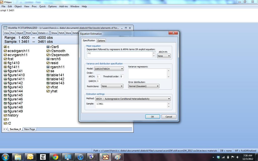
22 GARCH(1,1) 231 / 285

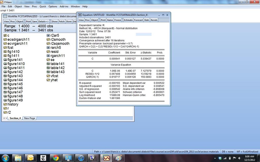
23 GARCH(1,1) 232 / 285

24 GARCH(1,1) Figure: Estimated Conditional Standard Deviation, Daily NYSE Returns. 233 / 285

25 GARCH(1,1) Figure: Conditional Standard Deviation, History and Forecast, Daily NYSE Returns. 234 / 285

26 Fancy GARCH(1,1) 237 / 285

27 Fancy GARCH(1,1) Dependent Variable: R Method: ML - ARCH (Marquardt) - Student's t distribution Date: 04/10/12 Time: 13:48 Sample (adjusted): Included observations: 3460 after adjustments Convergence achieved after 19 iterations Presample variance: backcast (parameter = 0.7) GARCH = C(4) + C(5)*RESID(-1)^2 + C(6)*RESID(-1)^2*(RESID(-1)<0) + C(7)*GARCH(-1) Variable Coefficient Std. Error z-statistic C 1.28E R(-1) Variance Equation C 1.03E E RESID(-1)^ RESID(-1)^2*(RESID(- 1)<0) GARCH(-1) T-DIST. DOF / 285

28 Nonstationarity and Random Walks Random walk: y t = y t 1 + ε t ε t iid(0, σ 2 ) Just a simple special case of AR(1) φ = / 285

29 Recall Properties of AR(1) with φ < 1 Shocks ε t have persistent but not permanent effects y t = φ j ε t j (note φ j 0) j=0 Series y t varies but not too extremely var(y t ) = σ2 1 φ 2 (note var(y t ) < ) Autocorrelations ρ(τ) nonzero but decay to zero ρ(τ) = φ τ (note φ τ 0) 251 / 285

30 Properties of the Random Walk (AR(1) With φ = 1) Shocks have permanent effects t 1 y t = y 0 + j=0 ε t j Series is infinitely variable E(y t ) = y 0 var(y t ) = tσ 2 lim var(y t) = t Autocorrelations ρ(τ) do not decay ρ(τ) 1 (formally not defined) 252 / 285

31 Random Walk with Drift y t = δ + y t 1 + ε t ε t iid(0, σ 2 ) y t = tδ + y 0 + t i=1 ε i E(y t ) = y 0 + tδ var(y t ) = tσ 2 lim var(y t) = t 250 / 285

32 Forecasting a Linear Trend + Stationary AR(1) x t = a + bt + y t y t = φy t 1 + ε t ε t WN(0, σ 2 ) Optimal forecast: x T +h,t = a + b(t + h) + φ h y T Forecast reverts to trend 7 / 40

33 Forecasting a Random Walk with Drift x t = b + x t 1 + ε t ε t WN(0, σ 2 ) Optimal forecast: x T +h,t = bh + x T Forecast does not revert to trend 6 / 40

34 Stochastic Trend vs. Deterministic Trend 9 / 40

35 A Key Insight Regarding the Random Walk Level series y t is non-stationary (of course) Differenced series y t is stationary (indeed white noise)! y t = ε t A series is called I (d) if it is non-stationary in levels but is appropriately made stationary by differencing d times. Random walk is the key I (1) process. Other I (1) processes are similar. Why? 253 / 285

36 The Beveridge-Nelson Decomposition y t I (1) = y t = x t + z t x t = random walk z t = covariance stationary Hence the random walk is the key ingredient for all I (1) processes. The Beveridge-Nelson decomposition implies that shocks to any I (1) process have some permanent effect, as with a random walk. But the effects are not completely permanent, unless the process is a pure random walk. 254 / 285

37 I (1) Processes and Unit Roots Random walk is an I (1) AR(1) process: y t = y t 1 + ε t (1 L) }{{} y t = ε t deg 1 One (unit) root, L = 1 y t is standard covariance-stationary WN More general I (1) AR(p) process: Φ(L) }{{} y t = ε t deg p [Φ (L) (1 L) }{{}}{{} ]y t = ε t (deg p-1)(deg 1) p 1 stationary roots, one unit root y t is standard covariance stationary AR(p 1) 255 / 285

38 Some Language... Random walk with drift vs. stat. AR(1) around linear trend unit root vs. stationary root Difference stationary vs. trend stationary Stochastic trend vs. deterministic trend I (1) vs. I (0) 8 / 40