CFD prediction of ship response to extreme winds and/or waves

Transcription

1 University of Iowa Iowa Research Online Theses and Dissertations Spring 2010 CFD prediction of ship response to extreme winds and/or waves Sayyed Maysam Mousaviraad University of Iowa Copyright 2010 Sayyed Maysam Mousaviraad This dissertation is available at Iowa Research Online: Recommended Citation Mousaviraad, Sayyed Maysam. "CFD prediction of ship response to extreme winds and/or waves." PhD (Doctor of Philosophy) thesis, University of Iowa, Follow this and additional works at: Part of the Mechanical Engineering Commons

2 CFD PREDICTION OF SHIP RESPONSE TO EXTREME WINDS AND/OR WAVES by Sayyed Maysam Mousaviraad An Abstract Of a thesis submitted in partial fulfillment of the requirements for the Doctor of Philosophy degree in Mechanical Engineering in the Graduate College of The University of Iowa May 2010 Thesis Supervisors: Professor Frederick Stern Associate Professor Pablo M. Carrica

3 1 ABSTRACT The effects of winds and/or waves on ship motions, forces, moments, maneuverability and controllability are investigated with URANS computations. The air/water flow computations employ a semi-coupled approach in which water is not affected by air, but air is computed assuming the free surface as a moving immersed boundary. The exact potential solution of waves/wind problem is modified introducing a logarithmic blending in air, and imposed as boundary and initial conditions. The turbulent air flows over 2D water waves are studied to investigate the effects of waves on incoming wind flow. Ship airwake computations are performed with different wind speeds and directions for static drift and dynamic PMM in calm water, pitch and heave in regular waves, and 6DOF motions in irregular waves simulating hurricane CAMILLE. Ship airwake analyses show that the vortical structures evolve due to ship motions and affect the ship dynamics significantly. Strong hurricane head and following winds affect up to 28% the resistance and 7% the motions. Beam winds have most significant effects causing considerable roll motion and drift forces, affecting the controllability of the ship. A harmonic wave group single run seakeeping procedure is developed, validated and compared with regular wave and transient wave group procedures. The regular wave procedure requires multiple runs, whereas single run procedures obtain the RAOs for a range of frequencies at a fixed speed, assuming linear ship response. The transient wave group procedure provides continuous RAOs, while the harmonic wave group procedure obtains discrete transfer functions, but without focusing. Verification and validation studies are performed for transient wave group procedure. Validation is achieved at the average interval of 9.54 (%D). Comparisons of the procedures show that harmonic wave group is the most efficient, saving 75.8% on the computational cost compared to regular

4 2 wave procedure. Error values from all procedures are similar at 4 (%D). Harmonic wave group procedure is validated for a wide range of Froude numbers, with satisfactory results. Deterministic wave groups are used for three sisters rogue waves modeling. A 6DOF ship simulation is demonstrated which shows total loss of controllability with extreme ship motions, accelerations and structural loads. Abstract Approved: Thesis Supervisor Title and Department Date Thesis Supervisor Title and Department Date

5 CFD PREDICTION OF SHIP RESPONSE TO EXTREME WINDS AND/OR WAVES by Sayyed Maysam Mousaviraad A thesis submitted in partial fulfillment of the requirements for the Doctor of Philosophy degree in Mechanical Engineering in the Graduate College of The University of Iowa May 2010 Thesis Supervisors: Professor Frederick Stern Associate Professor Pablo M. Carrica

6 Graduate College The University of Iowa Iowa City, Iowa CERTIFICATE OF APPROVAL PH.D. THESIS This is to certify that the Ph.D. thesis of Sayyed Maysam Mousaviraad has been approved by the Examining Committee for the thesis requirement for the Doctor of Philosophy degree in Mechanical Engineering at the May 2010 graduation. Thesis Committee: Frederick Stern, Thesis Supervisor Pablo M. Carrica, Thesis Supervisor Ching-Long Lin William Eichinger Jianming Yang

7 To my parents who made sacrifices for my education, and to my siblings, especially my sister who was my strength through hard times. ii

8 ACKNOWLEDGMENTS I would like to heartily thank people who made this thesis possible, especially my advisors Prof. Frederick Stern and Prof. Pablo Carrica for their interest, encouragement, guidance and support. I would also like to thank my colleagues in the ship hydrodynamics group at IIHR, especially Dr. Hamid Sadat-Hosseini and Dr. Tao Xing, for their ideas and helpful discussions. I am grateful to the members of my thesis committee, and Prof. George Constantinescu who was on the comprehensive exam committee, for their support and helpful advices. I am greatly appreciative to Dr. Claudio Lugni and Dr. Joseph Longo for kindly providing us with results and explanations of INSEAN and IIHR EFD studies. I would like to show my gratitude to IIHR staff for their efforts in creating a pleasant research environment. This research was sponsored by Office of Naval Research under Grants N and N under the administration of Dr. Patrick Purtell whose support is greatly appreciated. Computations were performed at the NAVY DoD Supercomputing Resource Center. iii

9 TABLE OF CONTENTS LIST OF TABLES...vii LIST OF FIGURES.....viii CHAPTER 1. INTRODUCTION Literature Review on Air Flow Studies Air Boundary Layer over Water Waves Wind Effects and Ship Airwake Studies Literature Review on Ship Motions in Waves... 7 CHAPTER 2. COMPUTATIONAL METHODS Overview of CFDShip-Iowa Versions 4.0 and Overview of Mathematical Models in the Code Governing Equations Coordinate Transformation Hydrodynamic Equations Turbulence Model Single-Phase Level-Set Free Surface Model Free Surface Boundary Conditions for Air Flow Motions Propeller Model Controllers Discretization Strategy Incoming Waves Modeling and Code Development Contributions of the Current Work Shallow Water Waves Hurricane Waves Treatment for Air over Waves Boundary and Initial Conditions The Potential Solution The Blending Function for IC and BC in the CFD Code Deterministic Wave Groups Three Sisters Waves iv

10 CHAPTER 3. SHIP AIRWAKE STUDIES Wave Induced Effects on Air Boundary Layer over 2D Waves Wind Effects on Ship Resistance, Maneuvering, Seakeeping and Controllability Simulation Design Ship Airwake Analysis Static Cases in Calm Water Dynamic Airwake due to Ship Motions in Waves Wind Effects on Forces, Moments and Motions Calm Water Static Computations Pure Sway PMM Computations Pure Yaw PMM Computations Pitch and Heave in Regular Head Waves DOF Autopilot Hurricane CAMILLE Simulations CHAPTER 4. DETERMINISTIC WAVE GROUPS FOR SINGLE-RUN RAO AND ROGUE WAVES Development and Validation of Harmonic Wave Group Single-Run Procedure for RAO Deterministic Wave Groups RW TWG HWG URANS CFD Computations Seakeeping RAO Procedures Multiple-Run RW Procedure Single-Run TWG Procedure Single-Run HWG Procedure Simulation Conditions Natural Frequency and Maximum Response Wave Groups Design Domain, Grid Topology and Boundary Conditions Verification and Validation Results Iterative and Run Length Convergence Verification Studies for TWG at Fr= Validation Studies for TWG at Fr= Comparison of TWG, HWG and RW Procedures v

11 4.1.7 HWG Computations at Fr=0.19, 0.28 and Three Sisters Rogue Waves Simulation CHAPTER 5. CONCLUSIONS AND FUTURE WORK REFERENCES 134 vi

12 LIST OF TABLES Table 3-1 Summary of wind over 2D waves simulations Table 3-2 Geometrical properties of model DTMB 5613 (ONR Tumblehome) Table 3-3 Basic grids and decomposition information for ship simulations Table 3-4 Summary of ship simulations at Fr=0.2 (Re water = ) for wind effects on resistance, maneuvering and seakeeping and ship airwake studies Table 3-5 Forces and moments exerted by air flow for regular head waves (ak=0.052, λ/l=1.33, Fr=0.2) with wind speeds U /U=± Table 3-6 Propeller information for ONR Tumblehome used in hurrican simulations Table 3-7 Summary of hurricane CAMILLE simulations Table 4-1 Model properties for the IIHR and INSEAN experiments Table 4-2 Simulation conditions, average run length uncertainties and CPU costs (Bold:V&V Conducted) Table 4-3 Boundary conditions for all the variables Table 4-4 V&V results for TWG at Fr= Table 4-5 Summary of previous URANS CFD studies using RW procedure Table 4-6 Error values for HWG and RW procedures Table 4-7 Basic grids and decomposition information for the three sisters simulation Table 4-8 Refinements and background grids information for the three sisters simulation vii

13 LIST OF FIGURES Figure 2-1 Sketch of the potential problem of two fluids of different current velocities with a progressive wavy interface Figure 2-2 Exact potential solutions for water and air (λ=0.5, ak=0.25, U=U =0) Figure 2-3 u-velocity contours for potential solution, initial condition using blending, and the CFD turbulent solution (U /C=+0.5, U=0) Figure 2-4 Free surface and u-velocity contours for wind over JONSWAP waves (U /C significant =+3, U=0); Left: initialization, Right: CFD turbulent solution Figure 2-5 Superposition of two linear wave trains propagating in constant water depth Figure 3-1 The domain and grid used for wind over 2D waves simulations Figure 3-2 u-velocity percent difference between turbulent and potential solutions for various U /C (U=0, ak=0.25, wave velocity C is from left to right)...65 Figure 3-3 Streamlines in a reference frame moving with wave velocity C for various U /C Figure 3-4 w-velocity contours for various U /C Figure 3-5 u-velocity contours in a reference frame moving with wave velocity C Figure 3-6 Contours of x-viscous term in the momentum equation for various U /C Figure 3-7 Contours of dp/dx term in the momentum equation for various U /C Figure 3-8 Contours of modeled Reynolds stress <-u w > for various U /C Figure 3-9 Outline of the overset grid system and location of the interface at an instant during a hurricane simulation Figure 3-10 Q=30 iso-surfaces, streamtraces, and x-vorticity contours for three static conditions (U /U=7) viii

14 Figure 3-11 Fourier reconstruction of unsteady airwake of ship moving in regular head waves and head winds at z=6m above the deck, where the helicopter blades rotate Figure 3-12 Fourier reconstruction of unsteady airwake of ship moving in regular head waves and head winds for a vertical plane at x/l= Figure 3-13 Hull pressure distribution and air forces and moments for β=0 and β=20 in head and following winds and β=0 in beam winds (U /U=7) Figure 3-14 Motions, forces and moments for static drift β=0, 10, 20 degrees in calm water (Fr=0.2) with wind speeds U /U= 0 and ± Figure 3-15 Forces, moments and motions for beam wind with wind speeds U /U=0, 2.8, 4.79, and 7 in calm water (Fr=0.2) Figure 3-16 Motions, forces and moments for pure sway maneuvering (β max =10 ) in calm water (Fr=0.2) with wind speeds U /U= 0 and ± Figure 3-17 Motions, forces and moments for pure yaw maneuvering (r max =0.3) in calm water (Fr=0.2) with wind speeds U /U= 0 and ± Figure 3-18 Motions, forces and moments for regular head waves (ak=0.052, λ/l=1.33, Fr=0.2) with wind speeds U /U= 0 and ± Figure 3-19 Trajectories, histories of yaw, roll and rudder angles, and yaw moment components for hurricane CAMILLE simulations at Fr= Figure 3-20 Histories of ship forward velocity, drift angle, and propeller RPS for hurricane CAMILLE simulations at Fr= Figure 3-21 Comparisons of trajectories and roll motions for all hurricane CAMILLE simulations Figure 4-1 CFD coordinates, domain and boundary conditions Figure 4-2 RW time histories and frequency spectra of input waves and output ship motions (Fr=0.34, λ=1.293) Figure 4-3 a) Superposed TWG (I=60) compared to Gaussian wave packet, Equation ( 4.11). b) Evolved waves at the end of the computational domain compared to linear superposition of elementary waves Figure 4-4 TWG time histories and frequency spectra of input waves and output ship motions at Fr= ix

15 Figure 4-5 HWG time histories and frequency spectra of input waves and output ship motions at Fr= Figure 4-6 Overset grid system on the hull and centerplane (every other grid point of the medium grid is shown) Figure 4-7 Free surface wave fields at an instant (t=7.8 in Figure 4-5) during the HWG computation at Fr= Figure 4-8 Heave and pitch RAOs compared with EFD data at Fr=0.34 (TWG results are from the medium grid and medium time-step computation). 120 Figure 4-9 Heave and pitch RAOs compared with EFD data at Fr= Figure 4-10 Heave and pitch RAOs compared with EFD data at Fr= Figure 4-11 Heave and pitch RAOs compared with EFD data at Fr= Figure 4-12 Outline of the overset grid system used in the three sisters simulation shown at an instant during the simulation Figure 4-13 Linear sketch of the wave group used to generate the three sisters waves Figure 4-14 Nonlinear evolution of the designed three sisters waves inside the computational domain (a near-breaking moment) Figure 4-15 Histories of ship speed and propeller RPS during the three sisters simulation Figure 4-16 Ship trajectory during the three sisters simulation Figure 4-17 Histories of ship heading and rudder angle during the three sisters simulation Figure 4-18 Histories of heave, pitch and roll motions during the three sisters simulation Figure 4-19 Histories of acceleration components during the three sisters simulation Figure 4-20 Ship and free surface at various instants during the three sisters simulation x

16 1 CHAPTER 1. INTRODUCTION Assessing operational performance and defining safe operating envelopes for ships due to environmental conditions, especially extreme winds and/or waves, is of increasing importance due to use of novel hull forms, more challenging conditions such as higher speeds, increased human and equipment safety regulations and cost to accomplish mission considerations. Traditionally the effects of winds and waves in ship design have been analyzed separately, i.e., airwakes are studied without consideration to waves and ship motions and waves are studied without consideration to winds. Ship airwake studies have only considered the above water portion of the ship using experimental fluid dynamics (EFD) in wind tunnels and viscous computational fluid dynamics (CFD). For CFD the no-slip condition is applied on the above water portion of the ship and either no-slip or symmetry plane conditions are applied on the calm water plane. Early studies focused on forces and moments and flow fields for design optimization of superstructures, empirical estimation of strong wind effects on maneuvering, and plumes. Studies that are more recent focus on mean and turbulent airwakes and their effects on onboard anemometry and interactions with aircraft, including vortex structures and flow control. No studies have yet considered effects of ship motions on airwakes or dynamic effects of winds on ship motions and controllability. Ship motions and waves studies seldom include wind, using towing tanks and/or wave basins and traditionally potential flow (PF) and more recently viscous CFD. Linear and non-linear regular, random and deterministic wave conditions and ship motions and load responses are of interest, including capsize. Experimental research has focused on

17 2 specification and generation of various wave conditions and measurements of ship motions and loads. PF research has in some cases considered non-linear effects, but with limited progress due to inability to model wave breaking and viscous effects. CFD has shown promise for ship motions, including nonlinear motions and capsize without and with winds. No studies have yet considered deterministic wave conditions, i.e., linear wave groups for single-run seakeeping and nonlinear extreme events such as rogue waves. This thesis extends previous CFD studies for the prediction of ship response to extreme winds and/or waves. Wind studies employ a semi-coupled air/water approach, with limitations to resolve wave breaking, bubbles and air entrapment. Appropriate windwave environmental far-field boundary conditions are derived and validated through wave effects on wind studies covering full range of relative wind and wave propagation velocities, including comparisons with available direct numerical simulation (DNS) solutions. Wind effects are studied in the absence of waves for calm water resistance and static and dynamic maneuvering. Wind/wave studies are carried out for regular and irregular wave ship motions, including in the former case wave effects on airwakes using Fourier series reconstructions and in the latter case controllability and course keeping in hurricane waves and winds. A single-phase level-set approach is used for windless waves and ship motions computations. Procedures are developed based on deterministic wave groups for improved single-run response amplitude operator (RAO) predictions, and results are validated with available EFD data, including a complete verification and validation (V&V) study for the transient wave group procedure. Linear wave groups are used to generate three sisters rogue waves by imposing inlet boundary conditions. Waves then are evolved in the computational domain with nonlinear behavior, including wave breaking.

18 3 The thesis is organized as follows. Sections 1.1 and 1.2 provide literature reviews covering ship airwake and motions and waves, respectively. CHAPTER 2 describes computational methods in the single-phase and semi-coupled air/water CFD codes with focus on modeling and code development contributions of this thesis, which include appropriate wind-wave environmental far-field boundary conditions and its use for the present applications, shallow water and hurricane waves and wind spectra, and deterministic wave groups for linear RAO and large-amplitude rogue waves applications. CHAPTER 3 and CHAPTER 4 cover the ship airwake and deterministic wave group studies, respectively. Lastly, CHAPTER 5 provides conclusions and recommendations for future work. 1.1 Literature Review on Air Flow Studies This section covers two topics: fundamental studies of air boundary layer flow over water waves as the incoming environmental flow to the ship, and experimental and CFD wind effects and ship airwake studies Air Boundary Layer over Water Waves The simplest theoretical approach to the problem of air flow over water waves is the exact potential solution of two fluids separated by a wavy interface (Lamb, 1932). Since potential flow is inviscid, there is a discontinuity on the tangential velocity on the free surface, forming a vortex sheet. Miles (1957) introduced a resonant interaction at the critical height, where the wind speed equals the wave speed C in a frame moving with the wave speed, an inviscid instability mechanism leading to the formation of a vortical force (Lighthill 1962). Viscous effects were analytically studied by Belcher & Hunt (1993) who explained that turbulent stresses in the air flow cause a thickening of the boundary

19 4 layer on the leeside of the waves, leading to asymmetric displacement of the streamlines without separation. The flow was divided into inner region near the wave surface, where the flow is strongly affected by turbulent shear stress, and outer region, essentially inviscid. Highly accurate DNS computations were recently performed for flows over complex moving wavy boundaries. Sullivan et al. (2000) used DNS to study wave growth mechanisms with wind blowing in the same direction of the waves. They found that the mean flow tends to follow the undulating moving wavy surface, except when a region of closed streamlines (cat s eye) centered about the critical layer height is dynamically significant. Water waves are not computed and the simulations are performed only for wind blowing in the same direction as waves. DNS computations were also presented for fish-like swimming to study drag reduction and propulsive efficiency (Shen et al., 2003). The problem is different from wind over water waves in that the horizontal orbital velocities are not imposed at the surface, leading to separation and therefore a slightly different physics. Results were presented for wind with and against the waves. They found that for wind against the waves, attached eddies are observed and turbulence plays an important role in the near-surface region. For wind with waves, however, they found that the turbulence intensity and Reynolds stress are less important compared to the wind against waves condition. Shen et al. (2008) presented coupled wave-wind simulations using high order spectral (HOS) method for waves and large-eddy simulation (LES) for wind. Wind in the same direction as wave was considered for which wind flow structures including critical layer and cat s eye, coherent vortex structures and wind pressure field were studied. Wind effects on wavefield evolution were considered for a JONSWAP spectrum and, although wave growth found insignificant, the distribution of coherent vortices in the wind was slightly altered.

20 Wind Effects and Ship Airwake Studies The Resistance Committee of the 25th international towing tank conference (ITTC 2008) reviewed wind effects and ship airwakes studies for the first time, stating that so far EFD has played a major role on the prediction of aerodynamic forces, while CFD has been mainly used for prediction of flow fields. Early EFD works were focused on air resistance and wind force on the superstructure, (Hughes 1930, Izubuchi 1932). Araki and Hanaoka (1952) presented results for typical models of train ferries, and the data were used by Nakajima (1952) to investigate the effect of wind on the maneuverability of the same ships. By using the data obtained in the EFD studies, efforts to model aerodynamic forces and moments to develop empirical formulae were initiated. For example, Isherwood (1972) proposed methods based on a linear multiple regression model for merchant ships, and by using the results, Inoue and Ishibashi (1972) investigated ship maneuverability and course stability. More recently, advancements in EFD techniques allow more realistic and complex wind and ship conditions. Blendermann (1995) performed wind-tunnel measurements in nonuniform airflow and proposed a method to estimate the wind loading on ships. Nimura et al. (1997) focused on a tanker in ballast condition and performed wind tunnel tests not only for forces but also for flow visualization. Wind tunnel experiments have been performed to study the influence of a ship airwake on aircraft operating nearby, and the reduction of both turbulence levels and downwash velocities in the ship airwake, which should improve pilot workload and helicopter performance. Shafer and Ghee (2005) presented a study of active and passive flow control over flight decks of small naval vessels to explore the problems related to unsteady flow fields and large mean velocity gradients of ship airwakes, which cause excessive pilot workloads for helicopter

21 6 operations in the vicinity of small naval surface vessels. Most EFD studies are carried out in wind tunnels, with very few are in water tanks. Most CFD studies compute the air phase only and focus on the prediction of flow rather than aerodynamic forces. Reddy et al. (2000) simulated turbulent air flow around a generic frigate shape using a commercial CFD code, studying wind directions of 0, 45 and 90 degrees. A slip boundary condition for the U and V velocity components is used for the water surface. Popinet et al. (2004) used an LES technique to investigate mean and turbulent fluctuations of air velocity around the research vessel Tangaroa. Zero gradient boundary condition was applied for the water surface and simulations were performed with relative wind directions varying from 0 to 360 degrees with increments of 15 degrees. Polsky (2002) and Czerwiec and Polsky (2004) used a laminar Navier-Stokes solver to simulate the unsteady flow field produced by the superstructure of a LHA-class US Navy ship with particular focus on the effectiveness of the bow flap. The two phase level set flow solver CFDShip-Iowa version 5.0 is developed for coupled air/water computations and validated against experiments for DTMB ship model 5512 restrained from motions with sinkage and trim fixed at the dynamic conditions at two Froude numbers (Huang et al., 2007b). A semi-coupled immersed boundary approach is used in CFDShip-Iowa version 4.5, which is significantly more robust and faster compared to fully coupled approach (Huang et al., 2007a & 2008). Computations are validated for 5512 at medium Froude number and presented for ship model ONR Tumblehome in no-wind calm water and autopiloted in environmental waves and wind conditions of Sea State 7 where the ship experiences broaching events and the effects of wind result in a less controllable ship.

22 7 1.2 Literature Review on Ship Motions in Waves Different wave conditions used for ship simulations in ocean environment include regular waves, irregular random waves and deterministic wave groups including transient waves. Seakeeping typically focuses on linear response of a ship to incoming waves by obtaining the transfer functions, also called RAOs. Regular waves (RW) are traditionally used for towing tank or potential flow results and, for a given ship speed, require individual runs for each of the encounter frequencies of interest to obtain the entire RAO curves. The focus has been on linear response, while very limited nonlinear studies are reported. The transient test technique was proposed by Davis & Zarnick (1964) and further developed by Takezawa and Hirayama (1976), originally as an EFD procedure. An arbitrary wave spectrum with sufficient energy in the relevant frequency range is designed with deterministic phases to focus waves at a point in time and space. The hull begins to advance in calm water, while at the opposite end of the tank the wave train is generated. Near the focusing point, the model starts to respond to the transient waves. The interaction time is short, and the experiment ends with the model running in quasicalm water. The short test and small wave elevation downstream of the focus point reduce problems with reflected waves. Clauss and Bergmann (1986) recommended Gaussian wave packets and presented results for three cases: a submersible, an articulated tower and a floating oil skimmer. The wave packets were generated in the tank by the superposition of individual Gaussian wave components. Clauss (1999) later developed nonlinear numerical procedures to predict the propagation of any arbitrary wave spectrum with applications to linear seakeeping tests as well as the design of freak waves. The transient test technique was used in the INSEAN wave tank for DTMB model 5415 and

23 8 the results were compared with regular and irregular tests using JONSWAP and Pierson- Moskowitz spectra with generally good agreement (Lugni et al., 2000). A careful, sufficiently long acquisition of the evanescent tail response was reported necessary to preserve information. Later, a trimaran made by assembling three Wigley hulls was also tested at INSEAN and results were compared with irregular experiments using JONSWAP spectrum again with good agreement (Colagrossi et al., 2001). Potential-flow Rankine panel method results based on the transient test technique were also presented by Colagrossi et al. (2001). Solutions were presented and compared with experiments for DTMB model 5415 and the Wigley trimaran. Computations were also performed for a container ship (S175) and the results were compared with experimental data from 17 th ITTC. Satisfactory agreement was shown between numerical and experimental results. Viscous CFD tools based on unsteady Reynolds averaged Navier Stokes (URANS) computations are becoming more common for seakeeping computations according to 25 th ITTC seakeeping committee report. The regular wave procedure has been used and validated with experiments. Sato et al. (1999) used a surface capturing density function method and a ship-fixed coordinate system to compute ship motions in regular head waves for the Wigley hull and the Series 60 model. Pitch and heave amplitudes and phase angles were compared against experiments and showed reasonable agreement. Hochbaum & Vogt (2002) used a two-phase level set method to compute the air-water flow around ships in incident waves. Computations for a C-Box container ship free to surge, heave and pitch in regular head waves were presented, and comparisons with experimental data showed good agreement for small amplitude motions. Orihara & Miyata (2003) presented a surface capturing method based on a density function and overset grid capability. Emphasis was placed on added resistance in waves, and

24 9 validation was performed through comparison with pitch and heave motion measurements for S175 container ship in regular head waves. Good agreement was shown for heave and pitch amplitudes as well as added resistance. Weymouth et al. (2005) studied pitch and heave for a Wigley hull in regular head waves using the surface tracking code CFDShip-Iowa version 3.0. Comparisons with experiments for a wide range of encounter frequencies and Froude numbers showed good agreement. A surface capturing single-phase level set method was developed in CFDShip-Iowa version 4.0 (Carrica et al., 2007a) and extended to include six degrees of freedom motions using overset grids that move with relative motion during the computation (Carrica et al., 2007b). Computations were performed for DTMB model 5512 in regular, small amplitude (ak=0.025) head waves with λ/l=1.5 at Fr=0.28 and Heave and pitch amplitudes and phase angles compared favorably with experimental data by Irvine et al. (2008). A grid verification study using three grids ranging from 0.38M to 2.96M grid points was carried out for the zeroth harmonic of the ship resistance at Fr=0.28. Monotonic convergence was achieved, but no data were available for validations. A solution for a large amplitude head wave case (ak=0.075) was also presented showing large amplitude nonlinear motions and breaking transom waves, causing strong amplitude damping with respect to smaller amplitude waves. Hu & Kashiwagi (2007) used a constrained interpolation profile (CIP)-based Cartesian grid method with an interface capturing scheme to study pitch and heave motions for a Wigley hull in regular head waves. The RAO results agreed well with experimental data, except at large wavelengths. Stern et al. (2008) used CFDShip-Iowa Version 4.0 for pitch and heave computations of BIW-SWATH in regular head waves at Fr=0.54, with small (ak=0.026) and medium amplitude waves (ak=0.052) at different encounter frequencies. Pitch and heave RAOs were found to compare reasonably well with experimental data. The KCS container ship

25 10 in regular head waves was studied experimentally and computationally using CFDShip- Iowa Version 4.0 by Simonsen et al. (2008). CFD computations were performed for medium Fr=0.26 at resonance and compared against experiments for pitch and heave amplitudes and phase angles, and total resistance. Good agreement was found for pitch and heave motions, but resistance was underpredicted. Wilson et al. (2008) used an unstructured incompressible free surface RANS solver for pitch and heave computations of the S175 in regular head waves at Fr=0.2. Results were presented for only one encounter frequency with small and large amplitude waves. Pitch and heave transfer functions from small waves compare reasonably with experimental data. Nonlinear phenomena such as bow slamming, forebody plunging, and water on deck were demonstrated for large amplitude waves. This same case was computed by Paik et al. (2009) allowing hull deformation, with good results. Castiglione et al. (2009) studied the response of high speed (Fr=0.45, 0.6 and 0.75) DELFT catamaran in regular head waves using CFDShip-Iowa Version 4.0 and compared with experiments for low wave steepness, ak= For each speed, a range of wavelengths was computed to study the maximum response conditions. The natural frequencies were calculated for each Froude number from calm water simulations of the catamaran free to heave and pitch after applying an initial pitching moment. The natural frequencies were found almost independent of Froude number. The empirical formula presented by Irvine et al. (2008) for natural frequency of monohulls was extended for catamarans and verified with the simulation results, with good agreement. The peak heave and pitch responses occurred at the resonant frequency for all Froude numbers simulated, with insignificant exciting force effects. The response amplitude peaks increased with Froude number, reaching their maximum at the highest speed. The effects of wave steepness were also studied for Fr=0.75, comparing the results for ak=0.025, 0.05 and 0.1. Linear behavior was shown

26 11 for large wavelengths (λ/l>1.9) in the range of steepness tested, while elsewhere the heave and pitch responses were nonlinear for the highest steepness. For extreme ship motions including broaching and surf riding, Carrica et al. (2008) presented irregular wave simulations using CFDShip-Iowa Version 4.0. Roll motions in regular waves were studied for extreme ship motions in large waves (Sadat-Hosseini et al., 2007). Parametric roll in head waves and pure loss of stability due to beam waves were studied and validated against towing tank EFD for the ONR Tumblehome model. Simulations showed a good agreement with EFD for the ship with bilge keels in beam waves and head waves. EFD tests and CFD head wave simulations exhibited no parametric roll for the model with bilge keels due to large roll damping. Appropriate conditions for head wave CFD simulations without bilge keels were carried out and parametric roll was predicted for a range of Froude numbers, and the effects of increased wave steepness, drift angle and smaller/larger GM were studied. Parametric roll in head waves for the ITTC A-1 Container ship was systematically studied including model experiments, potential flow theory and CFD (Umeda et al., 2008). CFD overestimated the amplitude of the measured metacentric height variation at low speed but well explained the existence of secondary peak due to its super-harmonics. Irregular wave simulations were presented for extreme ship motions including broaching and surf riding (Carrica et al., 2008). 6DOF URANS computations were presented for ONR Tumblehome in a sea state 8 with an irregular Bretschneider spectrum and autopilot to control heading and speed. Calculations were performed for two controller types, and a time step study was included for one of the cases in irregular waves. A large hydrostatic yaw moment caused by a wave overcoming the ship from the stern was found primarily responsible for initiating the broaching, while the instantaneous

27 12 conditions of rudder position and roll angle contributed to the turning moment broadside to the waves and loss of steering capability. Extreme wave events experiments were performed using deterministic wave groups for a Ro-Ro vessel in a rogue wave and a semisubmersible in the Draupner New Year Wave embedded in extreme irregular seas (Clauss, 2002). For the Ro-Ro experiment, Bretschneider spectrum was used with wave focusing to generate a high sea from astern and a Z-maneuvering motion was specified to the ship. The vessel was found to broach and finally capsize as the roll exceeded 40 and the course became uncontrollable. The semisubmersible experiment was numerically simulated using the program TiMIT (Time-domain investigations, developed at the Massachusetts Institute of Technology), a linear panel method program for transient wave-body interactions. For the drilling semisubmersible GVA 4000 free to pitch and heave, the numerical response to the impact was found larger than experiments, due to disregard of viscous/nonlinear effects.

28 13 CHAPTER 2. COMPUTATIONAL METHODS 2.1 Overview of CFDShip-Iowa Versions 4.0 and 4.5 CFDShip-Iowa version 4.0 is an unsteady single-phase level-set solver with dynamic overset grids for 6DOF motions (Carrica et al., 2007a; Carrica et al., 2007b). The code solves the URANS equations using a blended k ε/k ω model for turbulence, with capabilities for detached eddy simulation (DES) turbulence modeling. CFDShip- Iowa version 4.5 is based on version 4.0 and uses a semi-coupled air/water immersed boundary approach to compute air flows (Huang et al., 2007a & 2008). The water flow is decoupled from the air solution, but the air flow uses the unsteady water flow as a boundary condition. The method can be divided into two steps. At each time step the water flow is computed first with a single-phase method assuming constant pressure and zero stress on the interface. The second step is to compute the air flow assuming the free surface as a moving immersed boundary for which no-slip and continuity conditions are used to enforce velocity and pressure boundary conditions for the air flow. In this chapter, first the computational methods used in CFDShip-Iowa version 4.5 are described, which also cover the version 4.0 since the first step in the semi-coupled approach is identical to single-phase level-set computations for the water flow. The modeling and code development contributions of this work are explained next including the wave modeling and boundary conditions for nonlinear shallow water waves and hurricane waves, treatment of the wind over waves boundary conditions introducing a logarithmic blending function, and deterministic wave group modeling.

29 Overview of Mathematical Models in the Code In this section, the mathematical methods used in the CFDShip-Iowa code are summarized briefly and references are provided for details. All variables and properties are non-dimensionalized with the reference velocity and length, U and L, usually the ship s speed and length between fore and aft perpendiculars, and corresponding fluid properties (water or air). The dimensionless parameters, Re and Fr are: Re = ρ UL μ (2.1) Fr = U gl (2.2) where l=w for water and l=a for air. expressed as: Governing Equations The RANS momentum and mass conservation equations for either water or air are u t +u u = p + Re x x x u + u +S x x (2.3) u x =0 (2.4) where the piezometric pressure p and the effective Reynolds number Re are: p =p+ z Fr k, p= p ρ U (2.5)

30 15 Re = 1 Re +γ (2.6) with k the turbulent kinetic energy and γ the non-dimensional turbulent viscosity obtained from a turbulence model, and S a body force due, for instance, to a propeller model. The subscript abs stands for the absolute dimensional value of any property or variable Coordinate Transformation The governing equations are transformed from the physical domain in Cartesian coordinates (x,y,z,t) into the computational domain in non-orthogonal curvilinear coordinates (ξ,η,ζ,τ) (Thompson et al., 1985), where all cells are cubes with unit sides. A partial transformation is used in which only the independent variables are transformed, leaving the velocity components U in the base coordinates Hydrodynamic Equations The transformed mass conservation equation reads: 1 J ξ b U =0 (2.7) and the momentum equation: U τ + 1 J ξ U U = 1 J b p ξ + 1 J ξ 1 J Re b b U ξ +b U ξ +S (2.8) where U =b U is the contravariant velocity.

31 Turbulence Model Menter s blended k ε/k ω model of turbulence is used (Menter 1994). The dimensionless equations for γ, k and ω expressed in curvilinear coordinates are: γ = k ω (2.9) k τ + 1 J b U k ξ = 1 J ξ 1 J 1 Re +σ γ b b k ξ +S (2.10) ω τ + 1 J b U ω ξ = 1 J ξ 1 J 1 Re +σ γ b b ω ξ +S (2.11) with the corresponding sources: S =γ 1 J b U ξ +b U ξ b U ξ β ωk (2.12) S =γ γ ω k 1 J b U ξ +b U ξ b U βω ξ (1 F )σ ω J b k ω ξ b ξ (2.13) where the blending function is computed from: F =tan (α ) (2.14) α =min max k 0.09ωδ ; Re δ ω ; 4σ k CD δ (2.15)

32 CD =max 2σ ω J b k ω ξ b ξ ;10 (2.16) where δ is the distance to the wall, β =0.09, σ ω2 =0.856, and κ=0.41 are model constants, and σ k, σ ω, β, and γ=β/β -σ ω κ 2 / β are calculated by weight averaging the k-ω and the standard k-ε models with the weight coefficient F Single-Phase Level-Set Free Surface Model The 3D level set function, Φ, is defined in the whole domain with its value related to the distance to the interface. The sign of Φ is arbitrarily set to negative in air and positive in water and the iso-surface Φ=0 represents the free surface. Since the free surface is considered a material interface, then the equation for the level set function is: Φ t + (ΦU ) x =0 (2.17) A zero gradient velocity boundary condition is used: U. N = 0 (2.18) where N = is the unit normal vector to the free surface. As a good approximation on the water side, the pressure is taken as constant in the air. Neglecting surface tension, the pressure boundary condition is: p = z Fr (2.19) In addition, a zero normal gradient for both k and ω is used at the free surface:

33 18 k. N = ω. N = 0 (2.20) Details of the level set method used in CFDShip-Iowa including reinitialization techniques are described in Carrica et al. (2007a). zero: Free Surface Boundary Conditions for Air Flow The free surface is a moving no-slip boundary for air and the velocity jump is [U] =0 (2.21) The pressure at the interface is implemented by imposing the divergence free condition for the incompressible fluid combined with the immersed boundary method. Ghost pressures are adopted at all grids points that are first neighbors to the interface in the water region, including fringe points arising from overset grids. This approach makes the computation very stable because the forcing points in the air region close to the immersed boundary can be computed and corrected under a sharp interface condition. Similar to the situation in the water region, both k and ω are assumed to satisfy zero gradient normal to the free surface: k. ( N) = ω.( N) =0 (2.22) Details of the semi-coupled immersed boundary approach including the pressure equation in water points neighbor to the interface are described in Huang et al. (2007a & 2008).

34 Motions The 6DOF rigid body equations of motion are derived as 6 nonlinear coupled equations to represent the translational and rotational motions of a ship. To simulate moving rudders and other control surfaces or resolved propellers, a hierarchy of objects is used. The children objects (for instance the rudders) inherit the motions from the parent (the ship) and add its own motion respect to the parent object. The fluid flow is solved in the absolute inertial earth-fixed coordinates, while the rigid body equations of motion are solved in the non-inertial ship-fixed coordinates. Forces and moments are computed on the earth system by integrating piezometric pressure, friction and buoyancy separately on parent and children objects and then projected into the ship-fixed system. A second order implicit method with a predictorcorrector approach is used for solving the equations of motions. Rigid overset grids move with relative motion during the computation, and the interpolation coefficients between the grids are recomputed dynamically every time the grids move. 3 to 5 nonlinear iterations are performed at each time step to achieve converged fluid/motions solutions. It is important to mention that the grid velocity should be subtracted for the convection velocity in equations (2.3), (2.8), (2.10) and (2.11), and in the level set transport equation, (2.17). This grid velocity is imposed as the no-slip boundary condition on the ship hull. Details of the motions prediction including the overset method are described in Carrica et al. (2007b) for the single-phase code. For the semi-coupled code, the overset implementation is similar to that of the single-phase solver, with the difference that the pressure at the ghost points in water neighbor to the free surface is solved by imposing continuity even if they are fringe points. See Huang et al. (2007a & 2008) for details.

35 Propeller Model A prescribed body force model (Stern et al., 1988) is used to compute the propeller-induced velocities on the flow. This body force depends on the thrust and torque coefficients K T and K Q obtained from the open water curves of the propeller as a function of the advance coefficient, defined as: J= U nd (2.23) where n is the angular velocity of the propeller, D P is the propeller diameter and U is the velocity at the propeller location, approximated as the ship forward velocity. The radial distribution of forces is based on the Hough and Ordway circulation distribution, which has zero loading at the root and tip. A vertex-based search algorithm is used to determine which grid-point control volumes are within the actuator cylinder. The propeller model requires the input of thrust, torque and advance coefficients and outputs the torque and thrust force to the shaft and the body forces for the fluid inside the propeller disk. The force and torque of each propeller are projected into the non-inertial ship-fixed coordinates and used to compute an effective force and torque about the center of rotation, which is usually coincident to the center of gravity. The location of the propeller is defined in the static condition of the ship. When motions are involved, the propeller disk will move accordingly with the ship s motions Controllers Active and passive controllers are available to impose a variety of ramps in ship forward speed and propeller rotational speed, turning and zig-zag maneuvers, speed control (controlling a propeller body force model or a fully modeled rotating propeller), heading control (controlling rudder angle), autopilot (using simultaneously speed and

36 21 heading control) and waypoint control (using autopilot with variable heading). The controllers are either logical, based on on/off signals and limiting action parameters, or active proportional integral derivative (PID) type. Limiters of action use physical limits of the actuators to add reality to the resulting actuator setting. For instance, a rudder has a maximum and minimum operational angle, and a maximum allowed rudder rate. PID controllers involve three separate parameters; the proportional value that determines the reaction to the current error, the integral value that determines the reaction based on the sum of recent errors and the derivative value that determines the reaction to the rate at which the error has been changing. The weighted sum of these three actions is used to adjust the process using the classical action law: dψ dt =Pe+I edt +D de dt (2.24) where ψ is an action parameter, for instance the rudder angle, and e is the error of the controlled value respect to the target value (for instance heading respect to desired heading), given by: e=ψ ψ target (2.25) By tuning the three constants in the PID controller algorithm, the controller can provide control action designed for specific process requirements. variables: Discretization Strategy Second-order Euler backward difference is used for the time derivatives of all

37 22 φ τ = 1 τ (1.5φ 2φ +0.5φ ) (2.26) where φ is an arbitrary variable. The convective terms are discretized with a secondorder upwind method. Taking an arbitrary control volume P on the computational domain, the convection terms for variable φ can be written as: 1 J ξ U φ = 1 J [(C φ C φ ) + (C φ C φ ) + (C φ C φ )] (2.27) where u, d, w, e, s and n stand for the up (i-1/2), down (i+1/2), west (j-1/2), east (j+1/2), south (k-1/2) and north (k+1/2) faces of the control volume, respectively. At the down face, for example, we have: C = U (2.28) C φ = max(c,0)φ max( C,0)φ (2.29) φ =1.5φ 0.5φ (2.30) φ =1.5φ 0.5φ (2.31) Notice that the contravariant velocity in equation (2.28) has to be evaluated at the cell face, which is done by linear interpolation of the node values. The described convective discretization is applied for all the convective terms, including the momentum, turbulence and level set equations.

38 23 The viscous terms in the momentum and turbulence equations are computed with a second-order central difference scheme: 1 a φ J ξ Re ξ =D D +D D +D D (2.32) where a = b b J (2.33) and the diffusive flux in the down direction is: D = 1 J a Re φ ξ (2.34) The mass conservation is enforced using the pressure Poisson equation: ξ b b p b Ja ξ = ξ a a U, S (2.35) Incoming Waves For deep water calculations, waves are considered as a Gaussian random process and are modeled by linear superposition of an arbitrary number of elementary waves. Initial and boundary conditions are imposed in both water and air to generate the waves and wind inside the computational domain. In water, the initial and boundary conditions (free surface elevations, velocity components and pressure) are defined from the superposition of exact potential solutions (φ) of the wave components:

39 24 η(x, y, t) = a cos k xcosβ ysinβ ω t+φ (2.36) a φ(x, y, z, t) = e sin k xcosβ ysinβ ω t+φ Fr k (2.37) ω = k Fr +k cos β (2.38) where φ is a random phase, a is the wave amplitude, ω is the encounter frequency, k is the wave number, and β is the angle of incidence, all for the wave component with wavelength i and angle j. The maximum i and j are arbitrary numbers defined by the user. The angle of incidence is composed of the dispersion angle and the heading angle α of the ship: β =α +α (2.39) The wave amplitudes are computed from: a = 2S(ω )M(α )δωδα (2.40) where the directional M(α ) and frequency S(ω ) distributions depend on the chosen spectra. A cos 2 -type directional spectrum is used as: M α = 2 π cos α, π 2 <α < π 2 (2.41)

40 25 Bretschneider, Pierson-Moskowitz and JONSWAP spectra are implemented for frequency distributions, making the code capable of simulating a variety of sea states of interest, from mild to severe wave conditions. 2.3 Modeling and Code Development Contributions of the Current Work Shallow Water Waves For shallow water calculations, where the nonlinearities are significant, regular nonlinear waves are implemented into the code using the Stokes second-order perturbation theory: η(x, y, t) =a cos[k(xcosβ ysinβ) ωt] + a k cosh(kd) 4 sinh (kd) [2 +cosh(2kd)]cos{2[k(xcosβ ysinβ) ωt]} (2.42) φ(x, y, z, t) =a g cosh[k(d +z)] sin[k(xcosβ ysinβ) ωt] ω cosh(kd) + 3 cosh[2k(d + z)] 8 a ω sinh sin{2[k(xcosβ ysinβ) ωt]} (2.43) (kd) where d is the water depth Hurricane Waves Hurricane waves are implemented into CFDShip-Iowa code to compute the ship response to the environmental conditions imposed by hurricane waves and winds. The wave spectra of hurricane-generated seas have features, which are different from those of

41 26 ordinary storms. One of the features is that the energy of the wave spectrum of hurricanegenerated seas is concentrated around the modal frequency, in contrast to ordinary storms where the energy is spread over a wide frequency range or even double peaks. The results of all studies on hurricane-generated waves show that the wave spectra can best be represented in the form of the JONSWAP spectral formulation with different values for the parameters, called the modified JONSWAP spectral formulation (Foster, 1982): S(ω) = 4.5 (2π) g H ω ω e. ( 9.5 2π ω H. ) ( ) ( ) (2.44) where H is the significant wave height, ω is the modal frequency, σ is 0.07 for ω ω and 0.09 for ω >ω. Directional spreading of the hurricane waves is also different from ordinary storm waves. The dominant waves in a hurricane have a narrow directional spread within ±20 of the dominant direction. A cosine-fourth directional spreading function in a ± range, which is much narrower than the standard spreading for irregular ocean waves, is used herein: M α = 12 π cos ( 9 2 α ), π 9 <α < π 9 (2.45) Treatment for Air over Waves Boundary and Initial Conditions Development of CFDShip-Iowa version 4.5 required a proper treatment for air over water waves initial conditions (ICs) and boundary conditions (BCs) (Huang et al., 2007a), which was addressed as part of this thesis. A potential solution is obtained for air over water waves. Then a blending function is introduced to treat the discontinuity in the potential solution and admittedly

42 27 roughly represent the thin viscous layer above the water waves. The turbulent air boundary layer then develops inside the computational domain after enough time steps. It is worth noting that Sullivan et al. (2000) used a linear velocity profile above the water waves as ICs in their DNS calculations The Potential Solution Following Lamb (1932), the potential problem of two fluids of different densities (ρ and ρ ), one beneath the other, moving parallel to x with different velocities (U and U ) and with a progressive wavy interface is considered (Figure 2-1). The velocity potential function for each fluid, φ(x, y, z, t) and φ (x, y, z, t), are assumed to be: φ=ux+φ (2.46) φ = U x + φ (2.47) are: The kinematic free surface boundary conditions for the lower and upper fluids φ z = η t +U η x (2.48) φ z = η t +U η x (2.49) The dynamic free surface conditions derived from the Bernoulli equation by specifying constant pressure at the interface are:

43 28 φ t +U φ x + p ρ +gη=0 (atz=0) (2.50) φ +U φ t x + p ρ +gη=0 (atz=0) (2.51) Since the pressure must be continuous (p =p ) at the interface, equations (2.50) and (2.51) are combined into the following equation: ρ φ t +U φ x +gη =ρ φ +U φ t x + gη (at z = 0) (2.52) To find the solution, let us assume that the free surface (η) and the potential functions have the following forms: η=ae ( ) (2.53) φ = Ae [ ( )] (2.54) φ = A e [ ( )] (2.55) The kinematic boundary conditions, equations (2.48) and (2.49), yield: i(ku ω)a =Ak (2.56) i(ku ω)a = A k (2.57)

44 29 The dynamic free surface boundary condition, equation (2.52), results in: ρ{ia(uk ω) +ga} =ρ {ia (U k ω) +ga} (2.58) Combining equations (2.56), (2.57) and (2.58), the following equation is obtained: ρ(ku ω) +ρ (ku ω) =gk(ρ ρ ) (2.59) Solving equation (2.59) for ω gives: ω k = ρu + ρ U ρ+ρ ± g k ρ ρ ρ+ρ ρρ (ρ + ρ ) (U U ) (2.60) Finally, the potential functions will be: φ=ux+a U ω k e[ ( )] (2.61) φ = U x a U ω k e[ ( )] (2.62) The first term on the right-hand side of equation (2.60) may be called the mean velocity of the two currents. Relative to this there are waves traveling with velocities ±C given by: C = g k ρ ρ ρ+ρ ρρ (ρ + ρ ) (U U ) (2.63) Equation (2.63) shows that the presence of the upper fluid has the effect of diminishing the velocity of propagation of waves of any given wave-length. For air over water and U =U, the difference is only 0.1%. Even for the largest U U possible in

45 30 the ocean, under hurricane conditions and the most unfavorable k, the effect of the air flow on the wave frequency is only 1%. Therefore, in the current implementation the wave velocity is always C = g k, regardless of air density and velocity. The exact potential solutions for u, w and p in both water and air are shown, as an example, in Figure 2-2 for a regular wave with λ=0.5, ak=0.25 and U=U =0. From equations (2.61) and (2.62) it is clear, as also can be seen Figure 2-2, that the potential solution has a discontinuity at the interface. The normal velocity is of course continuous, but the tangential velocity changes sign across the surface, indicating the presence of a vortex sheet. In reality however, viscosity causes the tangential velocity to be continuous and the vortex sheet replaced by a film of vorticity The Blending Function for IC and BC in the CFD Code To treat the discontinuity in the potential solution when defining the boundary and initial conditions, a logarithmic blending function is used: u=u + (u u ) ln 2 ln Φ+δ δ (2.64) where Φ is the level set function, δ is the blending thickness defined by the user, u is the tangential velocity in the blending region, u is the potential tangential velocity of water at the free surface, and u is the potential tangential velocity of air at Φ =δ. For irregular waves, the same potential solution and blending function is used to define each elementary wave component in the superposition. As an example, Figure 2-3 shows the u-velocity contours from the potential solution, the initialization after applying the blending function, and the CFD turbulent solution for a regular wave with λ=0.5, ak=0.25 and wind velocity U /C=+0.5 in a frame

46 31 moving with current velocity U (therefore U=0). Comparing the initial and final solutions, it can be clearly seen that the final wave is nonlinear with flatter trough and steeper crest, due to the large ak. The potential solution is a good approximation for the water flow and for the air flow outside the turbulent boundary layer. The blending provides a smooth initialization for near surface air flow and, for this case of slow wind speed with no cat s eye region, it is even a roughly acceptable approximation. The air flow in the near surface region is however more complicated because it is dependent on U /C, as discussed in CHAPTER 3. Figure 2-4 shows u-velocity contours for the initialization and the CFD turbulent solution for irregular multidirectional JONSWAP waves with U /C significant =+3, again in a frame moving with the current velocity U. Note that in the turbulent solution the velocity distribution inside the boundary layer and the thickness of the layer itself varies with location and time (not shown), but outside the turbulent boundary layer, the superposition of the potential solutions is an acceptable approximation Deterministic Wave Groups Linear superposition of waves can be used to create not only random seas, but also deterministic wave groups for special purposes. The capability of reading an input waves file is implemented into the CFDShip-Iowa code, allowing superposition of any arbitrary number of waves with arbitrary frequencies, amplitudes and phases. One application is especially designed wave groups for single-run RAOs, as described in CHAPTER 4 along with transient and harmonic wave theories for linear seakeeping. The application of deterministic wave groups for generating three sisters rogue waves is addressed here.

47 Three Sisters Waves Two linear wave trains propagating in the x-direction with a small frequency difference Δσ and the corresponding wave number difference Δk are considered: η = H 2 cos k 1 2 Δk x σ 1 2 Δσ t (2.65) η = H 2 cos k +1 2 Δk x σ +1 2 Δσ t (2.66) The linear superposition of these two waves gives: η=η +η = Hcos(kx σt)cos 1 Δk x Δσ 2 Δk t (2.67) The individual waves in the resulting wave profile are bracketed within a wave envelope that also propagates forward. The envelope is defined by the last term on the RHS of equation (2.67). While waves within the envelope propagate at the speed of C=σ/k, the wave envelope propagates at a different speed, group velocity C g =Δσ/Δk. The wave energy is transmitted together with the wave envelope rather than the individual wave form. Finally, the nominal wavelength of the wave envelope is: L = 2π Δk 2 = 4π Δk (2.68) An example of the resulting wave profile is shown in Figure 2-5 for k=5.2, Δk=1.023, σ=7.67, Δσ=1.063 and H=0.16. By a proper design of the wave parameters, the surface profile in equation (2.67) can represent three sisters waves characterized by three consecutively large waves with small surface elevations prior to and after, as shown in CHAPTER 4.

48 33 Figure 2-1 Sketch of the potential problem of two fluids of different current velocities with a progressive wavy interface Figure 2-2 Exact potential solutions for water and air (λ=0.5, ak=0.25, U=U =0)

49 34 Figure 2-3 u-velocity contours for potential solution, initial condition using blending, and the CFD turbulent solution (U /C=+0.5, U=0) Figure 2-4 Free surface and u-velocity contours for wind over JONSWAP waves (U /C significant =+3, U=0); Left: initialization, Right: CFD turbulent solution

50 Figure 2-5 Superposition of two linear wave trains propagating in constant water depth 35

51 36 CHAPTER 3. SHIP AIRWAKE STUDIES In this chapter, the effects of wind on ship forces, moments, motions, maneuverability and controllability are investigated for the ONR Tumblehome model, characterized by a large superstructure. Airwake studies are carried out including the dynamic effects of ship motions in waves on the airwake flows. The semi-coupled approach, described in CHAPTER 2, is used for all computations. Water flow was unaffected by air flow, but air flow is computed considering the free surface as a moving immersed boundary. The method has limitations since the air/water interface is assumed at atmospheric pressure, and thus bubbles and wave breaking cannot be resolved. In addition, since the effect of the air flow on the water flow is neglected, small-scale phenomena such as wave generation, spraying, etc. cannot be simulated. Nevertheless, the method is very favorable for large-scale problems in the present work such as air flow around decks and superstructures because of its inherent robustness and efficiency compared to fully-coupled approaches. Results are presented for turbulent air flows over 2D water waves to validate the semi-coupled approach and illuminate the effects of waves on wind as an environmental flow approaching the ship. Ship computations are performed to investigate effects of various wind speeds and directions on static drift and dynamic maneuvers in calm water, pitch and heave in regular head waves, and 6DOF motions in irregular waves simulating hurricane CAMILLE. 3.1 Wave Induced Effects on Air Boundary Layer over 2D Waves Fully-developed ocean waves are generated by winds blowing for a long time over a long fetch with almost constant speed. Local winds can have different speed and

52 37 direction and have negligible effects on waves. The effects of waves on local air flow, however, can be significant. Dynamic wave effects on wind flows create complicated unsteady incoming wave/wind systems as they encounter ships. Air flows interact dynamically with the moving wave surface through different mechanisms depending on relative wind and wave velocities. These dynamic interactions significantly alter flow structures and turbulence intensities. To reach a greater physical understanding of incoming wind/wave flows is the purpose of this study. The results validate code development efforts by comparison with DNS simulations. Simulations are performed for an ak=0.25, air/water density ratio of , and an arbitrary wavelength λ=0.5, though this value is immaterial. The frame of reference moves with the water current velocity (U=0 in Figure 2-1). Therefore, the u-velocity is zero far away in water and is called U far away in air. Results for U /C= -3, -1.5, -0.5, +0.5, +1.5 and +3 are presented here. It is worth noting that U /C values for the ship in head waves computations, presented in the next sections, are +1.5 and The domain and the Cartesian grid used for the wind over 2D waves simulations are shown in Figure 3-1. The domain size is (L x, L y, L z-water, L z-air )=(4,4,2,2)λ. The grid size is , with equal grid spacing in the x and y directions, and clustered in the z direction to resolve free surface and near surface air flows. All simulations start from the exact potential solution everywhere in water and air, except in air near the water region where the logarithmic blending is applied, as described in CHAPTER 2. The same potential solutions modified by the blending function are used for the boundary conditions. The waves travel one wavelength every 100 time steps and the simulations stop upon acquisition of steady solution (in a frame moving with wave velocity C). Table 3-1 lists conditions for all wind over 2D waves simulations.

53 38 The percent difference between URANS computations and potential solutions for u-velocity are shown in Figure 3-2. Except at the viscous layer above the water surface, flows are irrotational in water and air and the potential solution is a reasonable approximation. Maximum difference occurs downwind of the wave crest for negative U /C values. For positive U /C, the maximum is at the wave trough. The thickness of the viscous layer, where viscous and turbulent effects are significant, is not a constant: it is usually smaller over the wave crest. Viscous effects are generally negligible beyond about kz=1.25 for U /C=±3, kz=0.65 for U /C=±1.5, and kz=0.4 for U /C=±0.5. To study the results, a relative frame moving with the wave phase speed C is chosen. In this reference system, particle paths and streamlines coincide. The wave surface in this frame is a streamline and is stationary over time. Fluid particles at the water surface have phase-dependent and time-independent velocities as: (u=-c+akc Cos(kx), v=0, w=akc Sin(kx)). All results will be shown in the relative frame of reference and wave velocity C is always from left to right. Streamlines, shown in Figure 3-3, follow the shape of the surface in the near surface region and flatten farther away. For U /C<1, streamlines are in negative direction everywhere, closer to each other above wave crests, and diverge beyond the crest. For U /C>1, a critical layer above the water waves, z cr where u-c=0, is shown by dashed lines. z cr is asymmetrical about x, being thinner on the windward side and thicker on the leeward. For U /C=+3 it is almost flat, while for U /C=+1.5 it tends to follow wave shape and extends slightly higher vertically. A region of closed streamlines, called a cat s-eye pattern, centers about the critical layer height for U /C=+1.5 and +3. Horizontally, cat s eye patterns extend over nearly the entire wavelength. The center of cat s eye is located above the wave trough for U /C=+3, and downwind the wave crest for U /C=+1.5. The cat s eye height is slightly greater for

54 39 U /C=+1.5. Cat s eye patterns do not descend to the surface, so there is no separation or re-attachment point at the surface (see e.g. Gent & Taylor, 1977). Reverse flows occur below the cat s eye where streamlines closely follow the shape of the surface. Just above the cat s eye, streamlines conform to the cat s eye shape and not the wave surface. The cat s eye pattern is thus important for flow dynamics, since slower moving fluids inside the eye act as obstacles, deflecting streamlines away from the wave surface. Cat s eye patterns in these simulations agree well with previous measurements (Hsu et al., 1981) and DNS simulations (Sullivan et al., 2000; Shen et al., 2003). Vertical velocity contours are shown in Figure 3-4. For U /C<1, w-velocity is positive (negative) upwind (downwind) of the wave crest. Below the critical layer for U /C>1, effects of reverse mean flow and water surface orbital vertical velocities produce positive (negative) w-velocity on the leeward (windward) side of the wave. Above the critical layer, streamlines follow the critical layer shape and like a stationary surface, w- velocity is maximum (minimum) upwind (downwind) of the peak in z cr,. For U /C=+3, vertical deflection of critical level is smaller than undulations of water surface and therefore w magnitude generated by the cat s eye above the critical layer is smaller than that below z cr. For U /C=+1.5, deflections of the critical level is large and the w magnitude above the critical layer induced by the cat s eye is larger than that below the critical layer induced by the wave surface. Contours of u-velocity, Figure 3-5, show two distinct patterns at all U /C values: the near surface region where a turbulent boundary layer develops above the water surface and the outer region where the flow is inviscid. In the outer region, maximum (negative) horizontal velocity occurs above the wave crest and minimum above the wave trough for U /C<1. For U /C>1, the outer region contours follow the shape of the cat s eye and the maximum u-velocity occurs above the peak of the cat s eye pattern and

55 40 minimum above its edges. In the inner region, there is a wake flow zone with momentum deficits beyond the wave crest for U /C<0. The wake region deflects the contours away from the wave surface and is largest for U /C=-3. Contours of the viscous and pressure terms in the x-momentum equation are shown in Figure 3-6 and Figure 3-7, respectively. For all U /C values, pressure gradients are dominant and extend beyond the viscous effects. For U /C<1, pressure gradients are minimum preceding the wave crest and maximum beyond it. The viscous term is maximum before the wave crest and minimum beyond it, where the wake region is located for U /C<0. For U /C=+0.5, the viscous term is significantly reduced and the wake region eliminated. The orbital velocity at the surface is on the order of akc, therefore 0.25C for the present cases. Wind speeds away from the surface are 0.5C. Orbital velocities thus play a significant role in flow dynamics. For U /C>1, the adverse pressure gradients cause cat s eye recirculation, and the viscous term is maximum below eye center and minimum at the trailing edge of the cat s eye pattern. For U /C<1, viscous and pressure effects are strongest at the wave surface. For U /C>1, however, minimum and maximum viscous and pressure terms are displaced vertically due to the presence of the cat s eyes. Quantitatively, minimum and maximum values for pressure and viscous terms are smaller for positive U /C values. This is expected since momentum exchanges are smaller when the waves and winds move in the same direction. For U /C>1, the viscous term is small at the center of the cat s eye and where pressure gradient values are significant. Therefore, cat s eye pattern may be considered an inviscid mechanism, as theorized by Miles (1957) and Lighthill (1962). The contours of modeled Reynolds stress, <-u w >, are shown in Figure 3-8. For U /C<0, <-u w > is maximum beyond the crest, where the wake region is located. For U /C=+0.5, <-u w > is at least an order of magnitude smaller than in any other case. This

56 41 laminarization effect, due to elimination of the free shear layer, is consistent with previous studies (e.g. Hudson et al., 1996; Techet 2001; Shen et al., 2003). For U /C=+1.5 and +3, turbulence intensity is reduced, compared to U /C=-1.5 and -3. Turbulent effects are least significant at the cat s eye center, beyond the crest for U /C=+1.5 and above the trough for U /C=+3. This is also consistent with the inviscid nature of the cat s eye pattern. Maximum Reynolds stress occurs beyond the cat s eye, i.e. above the trough for U /C=+1.5 and over the crest for U /C= Wind Effects on Ship Resistance, Maneuvering, Seakeeping and Controllability Simulation Design The DTMB model 5613, ONR Tumblehome, is simulated. Model dimensions and geometrical properties as tested at model scale (EFD static drift tests at IIHR) and equivalent full scales are listed in Table 3-2. The model is appended with bilge keels, skeg, twin rudders, and incorporates the superstructure and flight deck. Rudders are fixed except for hurricane simulations where rudders control heading. The original rudders on model 5613 have a small trunk attached to the hull and a large spade. The present simulations employ approximated full spade rudders with no trunk, leaving a small gap between the hull and spade. This simplifies grid generation and overset design for the moving rudders. The overset grid design (Figure 3-9) is comprised of eleven base grids. Two double-o boundary layer grids model hull starboard and port sides and the aft deck. The superstructure grid, constructed with an H-type topology, oversets the boundary layer grids. Skeg, starboard and port bilge-keels also use H topology and overset boundary layer grids. Double-O grids are used for the rudders. Cartesian background grid extends

57 42 to -0.6L< x <1.8L, -0.6L< y <0.6L and -0.8L< z <0.8L. The propeller shaft and supporting struts are not included in the computations. In Table 3-3, the grid system is summarized including domain decomposition and object hierarchy. The background grid is not subject to ship pitch, heave or roll motions, but follows the ship by surging, swaying, and yawing (for 6DOF hurricane simulations). The background grid is refined about the free surface, assuring reasonable refinement independent of ship motions. The other grids form the ship object and move with it following the motions computed. The ship computations, with the exception of those for the hurricane simulations, are listed in Table 3-4. Simulation conditions include calm water simulations with ship forward motions and head, following, and beam winds of different speeds; calm water computations with static drift and dynamic maneuvers and head and following wind; and regular head waves with head and following wind. The ship is generally free to pitch, heave and roll, except for symmetric cases without roll. These simulations are designed to guide experimental tests to be performed at IIHR-Hydroscience and Engineering, The University of Iowa. For all calculations, except for planar motion mechanism (PMM) calculations with 384 time steps per period, 250 time steps are performed per dimensionless second. Nonlinear iterations are performed within each time step to couple the motions, turbulence equations, free surface locations, velocities and pressure. Typically, four nonlinear iterations are performed per time step. The blended k-ω/k-ε turbulence model with shear stress transport (SST) is employed, which generally gives better results than other isotropic two-equation turbulence models when flows show separation (Menter, 1994). There are overset grids on the solid surfaces (bilge keels and skeg overset the hull), so a special treatment is adopted for regions where cells overlap to preclude

58 43 counting twice the same area or force. Weights from 0 to 1 are assigned to the cells to assure correct area, forces and moments integration. Static drift simulations are carried out with a constant drift angle, β, and results are presented for β=0, 10 and 20. PMM simulations include pure sway and pure yaw maneuvering conditions. In pure sway, the ship oscillates side to side tracing a sinusoidal path described by the equation: y= S, sin(ωt) (3.1) Sway velocity is defined as: v =y= ωs, cos(ωt) (3.2) The effective heading angle, β is then defined as: β =tan (y) (3.3) which reaches its maximum at PMM phase 0. β eff, max is 10 in the present simulations. For pure yaw, the ship follows the tangent of a sinusoidal trajectory. Sway and yaw are prescribed as: y= S, sin(ωt) ψ= ψ cos(ωt) (3.4) The yaw rate is then defined as:

59 44 ω =r =ψ=ωψ sin(ωt) (3.5) which reaches maximum at PMM phase 90. r max is 0.3 in the present simulations Ship Airwake Analysis Ship airwake studies are important for helicopter and aircraft operations as well as onboard anemometry. The air flow behind the superstructure and above the deck of the ONR Tumblehome is studied in this section. Similar vortical flow analyses are presented for calm water static and dynamic cases (Sakamoto et al., 2008) and regular head waves (Carrica et al., 2007) for the DTMB 5512, only on the water flow. The symbols used for motions are: σ=sinkage, τ=trim, z=heave, θ=pitch and φ=roll Static Cases in Calm Water Figure 3-10 shows Q=30 iso-surfaces, streamtraces, and x-vorticity contours for ship advancing with β=0 and β=20 in head winds and β=0 in beam winds. The Q isosurfaces are colored by relative helicity, showing the rotation direction of the vortical structures. Almost all superstructure sharp edges produce bluff-body vortices. The most massive recirculations occur aft of the superstructure and over the aft deck. For β=0 in head winds, two counter-rotating vortices form aft of the superstructure, extending almost to the stern. Toward the aft, the strength of the vortices decreases significantly. For β=20, the vortices shift to port. Fluid particles on the superstructure port side form a positive-rotating vortex starting near the center. This vortex shifts to port immediately aft of the superstructure and is significant for only a small portion of the

60 45 deck. Fluid particles starboard of the superstructure form another vortex with negative rotation. This vortex is near the deck surface, does not shift away and extends almost to the stern. It is therefore significant for most of the port side of the aft deck. Flow asymmetries and critical velocity gradients over the aft deck can present challenging conditions for helicopter operations. The forward speed of the ship deflects beam wind streamlines slightly to the aft. The large superstructure blocks air flow causing streamlines to rise significantly. On the starboard side, a large recirculation zone develops with relatively low pressure. Therefore, streamlines passing over the bow are deflected toward this zone. The strongest vortices are formed in the wakes of sharp edges on the portside of the superstructure and aft deck. Except immediately aft of the superstructure, vortex strength is significant only on the portside and air flows are asymmetrical over most of the aft deck Dynamic Airwake due to Ship Motions in Waves FFT reconstructions of unsteady airwakes for the Tumblehome moving in regular head waves are carried out and compared with static results from the calm water sinkage and trim simulation. Two sections are selected: the plane 6m above the deck, where helicopter blades rotate (Figure 3-11), and at x L =0.8 (Figure 3-12). For calm water simulations, the ship moves forward at Fr=0.2 in head winds (U =+6U), coincident with the first case in Figure Predicted sinkage and trim are σ= l and τ=0.046 o (bow-down), respectively. The head waves simulation conditions are set for regular waves with λ=1.33 and ak= The ship moves at Fr=0.2 in head winds with U =+6U and is free to pitch and heave. The 0 th harmonic of heave and pitch motions are z 0 = L (1.5% larger than calm water sinkage) and θ 0 =0.107 o bow down (132.6% larger than calm water trim). The

61 46 1 st harmonic amplitudes of heave and pitch are relatively large, z 1 = L and θ 1 =2.90 o. Due to ship motions, airwake vortical structures move periodically and the flow is very unsteady. Analysis incorporates two steps. Flow solutions at all times are first transformed from an earth-fixed coordinate system to a ship-fixed frame through rigidbody equations. Solutions are then transformed from time domain to frequency domain through FFT analysis of results at all grid points in the abovementioned sections. 0 th harmonics show the same trend and almost the same values as in calm water steady conditions for all variables. 2 nd harmonic amplitudes were significant for all velocity components. In the horizontal section, Figure 3-11, the mean flow vortical structures include, similar to static simulations discussed previously, two counter-rotating vortices detaching from the superstructure to reach beyond the step in the aft deck. The u-velocity is small in the centerplane, becoming negative immediately downstream of the superstructure, indicating recirculation. Towards the sides, u-velocity increases rapidly. The v-velocity is not significant in the centerplane due to symmetry, but shows large inward flows caused by recirculation. The w-velocity contours show fluid particles from the sides deflected downward approaching the center of the deck. Immediately aft of the superstructure, large upward w-velocities occur where small and large counter-rotating vortices (observable in x-vorticity contours) meet. Maximum 1 st and 2 nd harmonic amplitudes for the u-velocity are 31% and 14% of the ship forward speed, respectively. The v-velocity shows two regions at the sides of the deck where all harmonic amplitudes are large. Compared to the maximum 0 th harmonic amplitude, the maximum v-velocity amplitudes are 8.8% for the 1 st harmonic and 5.9% for the 2 nd.

62 47 The w-velocity is greatly affected by large-amplitude pitching and heaving. The 1 st harmonic is significant where 0 th and higher harmonics are not. The 1 st harmonic has maximum values to the sides of the maximum 0 th harmonic. For steady sinkage and trim solutions, two counter-rotating vortices meet in the centerplane, producing maximum downward velocities. For pitching and heaving, the two vortices separate to the sides and then return to the center during each wave period, shifting the 1 st harmonic away from the centerplane. As the two big vortices approach each other, they increase in strength and extend longitudinally to each direction, causing the small vortices immediately aft of the superstructure to weaken. Therefore, the 1 st harmonic in the vortical system immediately aft of the superstructure is more significant in the centerplane than on the sides. Compared to maximum 0 th harmonic amplitude, maximum 2 nd harmonic amplitude is 5.5%. The x-vorticity is greatly affected by ship motions as vortical structures move and interact dynamically. During each wave period, the two large vortices move back and forth and to the sides. When they are closest to each other, they are strongest and closest to the superstructure, weakening the smaller side vortices. The period of this mechanism is the same as the encounter period and significant in the 1 st harmonic. Compared to the static condition, the vortices in the 1 st harmonic contours are farther apart from each other and closer to the superstructure. Two significant regions are present in the downstream, due to longitudinal extension of vortical structures during each wave period. The two small vortices at the superstructure sides do not move significantly. Only their strength varies with ship motion. The 2 nd harmonic more closely resembles the 0 th harmonic. Compared to maximum 0 th harmonic, maximum 1 st harmonic is 16.6%, and maximum 2 nd harmonic is 7.1%.

63 48 For the x/l = 0.8 section (Figure 3-12), u-velocity shows 1 st harmonic amplitudes peaking at about 29% of the air free stream velocity. The 2 nd harmonic amplitudes are about half of the 1 st harmonics and peak high off the deck. The v-velocity shows 1 st harmonics associated with vortex motion, reaching amplitudes of about 10% of the 0 th harmonic amplitude. These fluctuations are mostly at the deck surface and near the boards. The 2 nd harmonic amplitude is, again, about half of the 1 st harmonic, but peaks near the deck. For vertical velocity, 1 st harmonics are large near the deck halfway between the centerplane and the ship sides, with a relatively strong 2 nd harmonic at the centerplane. The 1 st and 2 nd harmonic amplitudes of x-vorticity are 20% and 4.4% of 0 th harmonic amplitudes, respectively Wind Effects on Forces, Moments and Motions Severe wind effects on ship forces, moments and motions are studied for static drift at β=0, 10 and 20 degrees; PMM maneuvers; and pitch and heave in regular head waves. All simulations are carried out under both head and following wind conditions. Beam winds results are also presented for β=0. Wind speeds are large, equivalent to hurricane strength in full-scale. The symbols for forces and moments are: X=surge force, Y=sway force, Z=heave force, K=roll moment, M=pitch moment and N=yaw moment Calm Water Static Computations Figure 3-13 shows hull pressure distributions and the corresponding air forces and moments for β=0 with head, following, and beam winds, and β=20 in head and following winds. For head winds, a small high pressure region is observed in the aft deck where flows separated from the superstructure reattach. Pressure is negative on top of the

64 49 superstructure, generating an upward force and reducing sinkage. The pitching moment is negative, inducing a bow-down ship attitude. Similar trends are observed for following winds, but these winds push the ship forward. For β=20, the wind has a transverse component and pressure distribution is asymmetric. As a result, transverse forces and roll and yaw moments are induced. For beam wind conditions, forward ship speed gives wind flow a u-velocity component, producing x-forces and yaw moments. There is positive pressure on the superstructure portside and negative on the starboard, generating large transverse forces and roll moments. Figure 3-14 shows motions, forces, and moments for no-wind, head and following winds at β=0, 10 and 20 degrees. For no-wind cases, results are compared to EFD (roll prohibited). For β=0, simulations agree closely with EFD data. Differences in sinkage, trim, and Y are significant for β=20, since in the present simulations the ship is free to roll. The roll angles are relatively large, 6.2 for β=10 and 24 for β=20. Both sinkage and trim (bow-down) increase with drift angle. Due to oblique water flows, X, Y, and N increase with the drift angle, while X f /X p, Y f /Y p, and N f /N p decrease. Wind effects are presented as a ratio to no-wind conditions. Results can be explained by air pressure distributions shown in Figure Sinkage decreases for head and following winds due to suction pressure on top of the large superstructure. The ratio is most significant for β=0. For β=10, the oblique water flow induces a large suction force, rendering the effects of wind less significant. For β=20, the ratio is more critical than for β=10, perhaps due to the shape of the ship. Flows that are more oblique have greater effects on the superstructure pressure distribution than on the round hull, under water. Trim increases (bow down) for head and following winds. In both cases, the airinduced pitching moment is negative. In head winds, deck pressure is negative

65 50 downstream of the superstructure. For following winds, this is due to high pressures aft of the superstructure wall. Predictably, the ratio is smaller for larger drifts where oblique water flow effects become dominant. Roll angles decrease with head winds and increase with following winds. The wind effect ratio is smaller for β=20, due to more significant water effects. The x-force is significantly affected by winds. Head winds increase total resistance by 28% for β=0, 18% for β=10 and 4.5% for β=20. Following winds decrease total resistance by 23% for β=0, 16% for β=10 and 10% for β=20. X f /X p shows that for following winds for β=0, total pressure drag is negative. Water pressure component is only 20% of water resistance. Air pressure and friction components are similar and very close to pressure drag in water. For this case of strong following winds, negative air drag force is so large as to render net pressure drag negative, though very small. Friction force is also negative for following winds, although the absolute value is only 40% of the head wind case due to the vast separated flow region. For β=10 and 20, X f /X p increases for following winds. The ratio, however, decreases with drift angle as pressure drag in water increases. For head winds, X f /X p decreases by 50% for β=0, 35% for β=10 and 4% for β=20. Y forces decrease under following winds and increase for head winds by 5% and 14%, respectively, for β=10 and 3.4% and 4.2% for β=20. As can be seen also in Figure 3-13, head winds produce larger pressure differences between port and starboard. Yaw moment, N, increases for both head and following winds. The ratio is larger for β=10 than for β=20. Head winds have greater effects on N, due to larger pressureinduced moments (Figure 3-13). Beam wind results are presented in Figure X force increases with increasing U /U. This may be due to ship forward speed and the geometry, producing a force in x

66 51 under side winds (negative lift). X f /X p decreases, showing, as expected, that beam winds produce more pressure drag than friction. Y force is a wind function, large due to the large superstructure. The Y/X ratio is 0.45 for U /U =2.8, 1.11 for U /U=4.7 and 2.03 for U /U=7. Y f /Y p is very small, decreasing as U /U increases, demonstrating that Y force is essentially pressure drag. The same trend is observed for N and N f /N p. Sinkage decreases with increasing U /U. Trim also decreases, possibly due to low forebody pressure. The roll angle induced by beam winds is 0.52 for U /U=2.8, 1.25 for U /U=4.7 and 2.52 for U /U=7. The roll angle may be the reason for downward trim and negative sinkage wind effects Pure Sway PMM Computations Pure sway results are presented in Figure The primary frequency for roll, Y, and N is the PMM frequency, f. The primary frequency for heave, pitch, and X is 2f. 0 th, 1 st, and 2 nd harmonic amplitudes of heave motion decrease for both head and following winds, consistent with the negative sinkage effects observed in the static case. This is a function of suction pressure forces over the deck and superstructure, larger for head winds, as previously discussed. The 0 th harmonic amplitude of pitch motion increases 0.4% for head winds and decreases 8.5% for following winds, in contrast to static trim increasing for all drift angles. The 1 st harmonic amplitudes decrease and 2 nd harmonic amplitudes increase for head and following winds. For roll motions, 0 th harmonic amplitude remains unchanged. All higher harmonic amplitudes decrease for head and following winds, with head wind effects stronger. When the ship moves left (right), roll angle is positive (negative). Relative wind speeds have a transverse component to the right (left), producing negative (positive) roll moments. The 0 th harmonic amplitude of X increases 21.7% for head winds

67 52 and decreases 16.6% for following winds. 1 st and 2 nd harmonic amplitudes of X decrease for head winds and increase slightly for following winds. Amplitudes of 1 st and all higher harmonics of Y forces increase for head and following wind conditions, following wind effects being larger. All N harmonics increase for head winds and decrease for following winds. This reflects the fact that water and air flows are in the same directions for head winds and in opposite directions for following winds Pure Yaw PMM Computations Pure yaw results are presented in Figure th harmonic amplitudes of heave decrease for both head and following winds. The 1 st harmonic amplitude decreases in head winds and increases in following winds, contrasting with negative sinkage effects for head and following winds for all drift angles (Figure 3-13). The 0 th amplitude of pitch increases 1.3% in head winds and decreases 10.9% in following winds. The 1 st harmonic amplitude decreases 8.4% in head winds and increases 4.4% in following winds. The 1 st and all higher harmonic roll amplitudes decrease in head winds and increase in following winds significantly, the reason being when the roll moment from water is positive (negative), the roll moment from air is positive (negative) in following winds and negative (positive) in head winds. The 0 th harmonic amplitude of X force increases 22.9% in head winds and decreases 17.4% in following winds. The 1 st harmonic amplitude decreases 11.2% in head winds and increases 4.5% in following winds. The 1 st and all higher harmonic amplitudes of the Y force increase in head winds and decrease significantly in following winds, the reason being Y forces from air and water are always in the same direction for head winds and in opposite directions for following winds. The 1 st and all higher harmonic amplitudes of N increase in head and following winds, following wind effects being larger.

68 Pitch and Heave in Regular Head Waves Regular head waves computations are carried out at λ/l=1.33, 0.78, and 0.5 for windless conditions. Results showed maximum response for λ/l=1.33, which was then selected for head and following wind computations. Wind results are shown in Figure 3-18 and Table th harmonic heave and pitch amplitudes are only 7.6% and 4.4% of the 1 st harmonic amplitudes, respectively. Therefore, they do not change meaningfully in response to head and following wind conditions. 0 th harmonic heave and pitch amplitudes are 108% and 148% of calm water static sinkage and trim, respectively. The 1 st amplitudes of heave and pitch decrease 0.4% and 0.1% for head winds and increase 0.5% and 0.7% for following winds. These numbers are within computational error margins. For following winds, Z a is maximum at t/t=0.53 where ship heave is minimum. Head wind Z a is maximum at t/t=0.27 where pitch is maximum (bow-up). The 0 th and 1 st amplitudes of Z a are about 61% and 129% larger, respectively, for following winds, resulting in stronger lift effects. The 2 nd amplitude of Z a is about 27 (%1 st ) and 43 (%1 st ) for head and following winds, respectively. Following winds M a are also larger than head winds: 690% for 0 th and 1227% for 1 st amplitudes. The 2 nd amplitude of M a is about 51 (%1 st ) and 30 (%1 st ) for head and following winds, respectively. M a maximums and minimums correlate to pitch motions. X force 0 th and 1 st harmonic amplitudes increase by 11.1% and 1.1% for head winds and decrease by 9% and 1.5% for following winds, respectively. The absolute value of air resistance, X a, is largest as the ship climbs waves at t/t=0.28. The 0 th and 1 st amplitudes of X a are about 13% and 246% larger, respectively, for following winds. The 2 nd amplitude of X a is about 44 (%1 st ) and 39 (%1 st ) for head and following winds, respectively.

69 DOF Autopilot Hurricane CAMILLE Simulations Hurricanes are one of the severest environmental conditions due to focused wave spectra, mighty winds and shifting wave and wind directions relative to ship headings and locations within the storm vortex. CFD simulations of wave and wind effects generated during hurricane CAMILLE are presented and ship controllability discussed in this section. A speed controller and autopilot set speeds and headings. Model 5613 ONR Tumblehome uses two counter-rotating propellers inboard on top. A prescribed body force model, based on an actuator disk approach, computes propeller-induced velocities on the flow, as described in CHAPTER 2. Since the propeller is only partially within the boundary layer, as a first approximation, wake factor and thrust deduction corrections are ignored and ship velocity is used to compute the advance coefficient. Stock propeller curves and diameter are employed since model propeller data are not available. Open water curves are expressed as second-order polynomials. The actuator disk location and thickness is prescribed with a vector transcribed from point P 1 to P 2, with radius r p and hub radius r h. Propeller details are provided in Table 3-6. An important extreme motion effect is the emergence of propellers from the water. A first-order approximation is applied where thrust and torque correspond to portions of the propeller below the water surface. Heading is controlled by rotating rudders through a vertical axis on the ship coordinate system passing through the point x= l, y=± l. PID-type controllers model an autopilot, controlling heading and speed simultaneously. PID controllers were described in CHAPTER 2. The exact parameters for hurricane CAMILLE simulations are herein defined.

70 55 Speed controller error is defined as the difference between instantaneous and target ship speeds: e =U U (3.6) The controller changes the propeller rotation speeds with the PI law: n=pe +I e dt (3.7) Heading controller error is defined as the difference between yaw angles and target headings: e =ψ ψ (3.8) The controller changes rudder angle as: dδ dt =Pe +I e dt (3.9) In the present simulations, non-dimensional controller constants are P= and I= Hurricane CAMILLE struck the Gulf of Mexico in It was one of the most intense U.S. hurricanes recorded (NOAA, 2006). CAMILLE is also the only Atlantic hurricane, and one of only four tropical cyclones worldwide, with wind speeds as high as 190 mph (85 m/s). Antani (1981) demonstrated that waves generated in hurricane CAMILLE could be represented with good accuracy by the modified JONSWAP spectrum, introduced in CHAPTER 2. Hurricane CAMILLE significant wave height and modal frequency were 13.2 m and 0.53 rad/s, respectively (Ochi, 2003).

71 56 For the ONR Tumblehome moving in hurricane CAMILLE at Fr=0.2, the most probable wave length is λ/l=1.42 and the wind speed is U /U=10.9. Resulting waves are of large amplitude and non-linear. In the computations, waves are generated inside the domain by imposing linear superposition of the waves as unsteady inlet boundary conditions. Waves thus distort within the domain as they evolve into non-linear waves. Relative dominant wave and local wind directions vary for various zones within the hurricane system. In the present simulation, the ship is assumed to move through a region forward of the advancing hurricane eye, where waves propagate in radial directions roughly perpendicular to local winds (Young 2006). The ship heading is assumed to encounter waves at an angle 135 to the ship (quartering seas from the stern on the starboard) with the perpendicular winds from 45 and 225. The ship travels almost 10 ship lengths during the simulations, for which it is assumed that the ship remains within the same region of the hurricane system, since the hurricane vortex diameter is of an order of 1300 ship lengths. Initially, two simulations were carried out at Fr=0.2. Two more simulations at a higher Froude number (Fr=0.35) were designed and carried out later to help understand and explain the results. Herein, the discussions are put in the same order, i.e. Fr=0.2 results are presented first. Table 3-7 summarizes all hurricane CAMILLE simulations. Yaw, roll, and rudder angle histories for Fr=0.2 simulations are shown versus non-dimensional seconds along with trajectories in Figure All time histories (Figure 3-19 and Figure 3-20) have been smoothed by filtering out high frequency oscillations introduced by shorter wavelengths. Very different scenarios for 45 and 225 wind conditions are observed. Beam wind components result in positive mean roll angles for 45 wind and negative angles for 225 wind (the sign is changed in Figure 3-19 for easier comparison with the 45 case).

72 57 The roll angle is higher for the 225 wind case, with local averages well above 20 after the first 10 dimensionless seconds, shortly after commencing the excursion to port. Roll angles reach up to 60, not shown in Figure 3-19 since frequencies higher than roll natural frequency are filtered. The controller changes rudder angles to maintain a ship heading of 0. The trajectory shows that in 45 wind, the ship drifts to port but is controllable with some loss of stability. For 225 wind, however, the ship loses control totally, turning 90 to port. A possible cause is the wind-induced roll angle against the wind, causing the ship to yaw into the wind. For 225 wind, hydrostatic and air yaw moments are initially negative, although the total moment is positive. At about 5 dimensionless seconds, an excursion begins, turning the ship to port. Though the rudder attempts a course correction by turning full to starboard, the ship cannot be recovered. The hydrostatic moment always turns the ship broadside to the waves, changing sign as the ship momentarily enters following seas in a turn from quartering seas, from starboard to port. The rudder always introduces a negative yaw moment. The wind starts with a small positive yaw moment. It becomes negative after 15 dimensionless seconds, as wind direction, with respect to the ship, becomes dominantly head winds on the port. Propeller controller results are shown in Figure Ship target speed is 0.4, corresponding to Fr=0.2. For the 45 wind case, the controller is turned on after t=5 s. It is on from the outset for the 225 wind case. The results show ship speed is controllable for both cases, oscillating around the target speed. Controller gain appears too large, as strong external excitation causes a propeller RPS change at the maximum rate. Velocity excursions are very large due to wave surfing, reaching velocities up to 50% over the target.

73 58 Figure 3-20 shows strong drifts caused by winds surpassing wave-induced drift. Negative drift results for winds from 45. Positive drift occurs in the 225 wind case, where drifts reach excursions over 25. These excursions correlate well with the velocity, once the ship reaches a quartering seas condition from port, as waves push the ship starboard. The correlation is negative for the 45 case and at the outset of the 225 wind case, suggesting wave surfing phenomena. Different wind directions can have opposite effects on ship controllability. For quartering seas from starboard, broaching events may be expected for this geometry, as presented for the absence of air forces by Carrica et al. (2008). In the 45 case, however, winds appear to stabilize the ship. With winds from 225, the ship loses control completely, culminating in total loss of steering capability, a very dangerous situation. Additional simulations were performed at a higher Fr=0.35, where control was expected to improve due to higher rudder moments, to help explain the nature of the controllability issues. Simulations were carried out with winds from 225, for which uncontrollability was observed at Fr=0.2, and without winds. Wave conditions were as in the Fr=0.2 simulations. Results are presented in Figure Trajectories show that for the no-wind simulation at Fr=0.35, the ship remains under control and sustains the target course despite hurricane waves. The situation for the 45 wind case performed at Fr=0.2 is similar, except that the ship moves to port, due to beam winds from starboard. Note that the beam components of wave and wind forces are in the same direction for the wind 45 case. For the wind 225 cases, where wave and wind forces have opposing beam directions, however, starkly different scenarios are observed. Excursions to port occur as the ship loses controllability. Although despite Fr=0.2 the propellers are able to reverse the excursion at Fr=0.35, zig-zag movements

74 59 occur with huge and abrupt roll motions (Figure 3-21). The results exhibit the significance of wind forces on route controllability and ship motions.

75 60 Table 3-1 Summary of wind over 2D waves simulations U /C ak C U Re=U λ/ν

76 61 Table 3-2 Geometrical properties of model DTMB 5613 (ONR Tumblehome) ONR Tumblehome Model Scale Full Scale L (m) B (m) T (m) L CG (m) Z CG (m) K xx K yy =K zz aft of FP above WL aft of FP 2.42 above WL Table 3-3 Basic grids and decomposition information for ship simulations Grid Points Processors Object Child to Boundary Layer Starboard 351,616 3 Ship None Boundary Layer Port 351,616 3 Ship None Super Structure 466,032 4 Ship None Skeg 118,188 1 Ship None Bilge Keel Starboard 119,556 1 Ship None Bilge Keel Port 119,556 1 Ship None Rudder Starboard Outboard 120,048 1 Ship Ship Rudder Starboard Inboard 120,048 1 Ship Ship Rudder Port Outboard 120,048 1 Ship Ship Rudder Port Inboard 120,048 1 Ship Ship Background 1,759, None None Total 3,766,511 32

77 62 Table 3-4 Summary of ship simulations at Fr=0.2 (Re water = ) for wind effects on resistance, maneuvering and seakeeping and ship airwake studies Case No. Conditions Wind-speed/Ship-speed U /U Re air Motions 1,2,3,4 Straight Ahead 0, +7, -7, , σ, τ 5,6,7 Straight Ahead Beam; 2.8, 4.7, , , σ, τ, φ 8,9,10 Static Drift, β=10 0, +7, σ, τ, φ 11,12,13 Static Drift, β=20 0, +7, σ, τ, φ 14,15,16 Pure Sway, β max =10 0, +7, z, θ, φ 17,18,19 Pure Yaw, r max =0.3 0, +7, z, θ, φ ,23,24 Reg. Head Waves λ/l=0.5, ak=0.125 Reg. Head Waves λ/l=0.78, ak=0.052 Reg. Head Waves λ/l=1.33, ak= z, θ 0 - z, θ 0, +6, z, θ

78 63 Table 3-5 Forces and moments exerted by air flow for regular head waves (ak=0.052, λ/l=1.33, Fr=0.2) with wind speeds U /U=±6 0 th Harmonic [-] 1 st Harmonic (%0 th ) 2 nd Harmonic (%1 st ) X a Head Following Head/Following (%) Z a Head Following Head/Following (%) M a Head Following Head/Following (%)

79 64 Table 3-6 Propeller information for ONR Tumblehome used in hurrican simulations Starboard Port K T J J J J 2 K Q J J J J 2 r p /L r h /r p P 1 /L ( , , ) ( , , ) P 2 /L ( , , ) ( , , ) Table 3-7 Summary of hurricane CAMILLE simulations Fr Re water Wind-speed/Ship-speed U /U Re air Wave Direction (Deg) Wind Direction (Deg)

80 65 Figure 3-1 The domain and grid used for wind over 2D waves simulations Figure 3-2 u-velocity percent difference between turbulent and potential solutions for various U /C (U=0, ak=0.25, wave velocity C is from left to right)

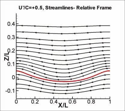
81 66 Figure 3-3 Streamlines in a reference frame moving with wave velocity C for various U /C Figure 3-4 w-velocity contours for various U /C

82 67 Figure 3-5 u-velocity contours in a reference frame moving with wave velocity C Figure 3-6 Contours of x-viscous term in the momentum equation for various U /C

83 68 Figure 3-7 Contours of dp/dx term in the momentum equation for various U /C Figure 3-8 Contours of modeled Reynolds stress <-u w > for various U /C

84 69 Figure 3-9 Outline of the overset grid system and location of the interface at an instant during a hurricane simulation

85 70 Figure 3-10 Q=30 iso-surfaces, streamtraces, and x-vorticity contours for three static conditions (U /U=7)

86 71 Figure 3-11 Fourier reconstruction of unsteady airwake of ship moving in regular head waves and head winds at z=6m above the deck, where the helicopter blades rotate

87 72 Figure 3-12 Fourier reconstruction of unsteady airwake of ship moving in regular head waves and head winds for a vertical plane at x/l=0.8

88 73 Figure 3-13 Hull pressure distribution and air forces and moments for β=0 and β=20 in head and following winds and β=0 in beam winds (U /U=7)

89 74 Figure 3-14 Motions, forces and moments for static drift β=0, 10, 20 degrees in calm water (Fr=0.2) with wind speeds U /U= 0 and ±7

90 75 Figure 3-15 Forces, moments and motions for beam wind with wind speeds U /U=0, 2.8, 4.79, and 7 in calm water (Fr=0.2)

91 76 Figure 3-16 Motions, forces and moments for pure sway maneuvering (β max =10 ) in calm water (Fr=0.2) with wind speeds U /U= 0 and ±7

92 77 Figure 3-17 Motions, forces and moments for pure yaw maneuvering (r max =0.3) in calm water (Fr=0.2) with wind speeds U /U= 0 and ±7

93 78 Figure 3-18 Motions, forces and moments for regular head waves (ak=0.052, λ/l=1.33, Fr=0.2) with wind speeds U /U= 0 and ±6

94 79 Figure 3-19 Trajectories, histories of yaw, roll and rudder angles, and yaw moment components for hurricane CAMILLE simulations at Fr=0.2

95 80 Figure 3-20 Histories of ship forward velocity, drift angle, and propeller RPS for hurricane CAMILLE simulations at Fr=0.2

96 81 Figure 3-21 Comparisons of trajectories and roll motions for all hurricane CAMILLE simulations

97 82 CHAPTER 4. DETERMINISTIC WAVE GROUPS FOR SINGLE-RUN RAO AND ROGUE WAVES Deterministic wave groups are used for both single-run linear seakeeping computations and rogue wave event simulations. Harmonic wave group single-run seakeeping procedure is developed, validated with EFD data from two facilities and compared with conventional regular waves and transient wave group procedures for DTMB model The single-run procedures obtain the response amplitude operators (RAO), which are ultimately used to determine the safe operating envelopes (SOE), in a single simulation for each ship speed. A rogue wave simulation is demonstrated for 6DOF motions of an autopiloted ONR Tumblehome in a three sisters event. In this chapter, all simulations are carried out using the single-phase CFD code and wind flows are not computed. 4.1 Development and Validation of Harmonic Wave Group Single-Run Procedure for RAO Single-run procedures give the RAO for a range of encounter frequencies by analyzing the response of the ship advancing at constant speed to an incoming wave system with enough energy in that frequency range. Procedures based on irregular waves with random phase shifts between the superposition of component waves require very long runs to limit scattering in the statistical analysis of the results. Deterministic wave groups, which are the focus of the present work, are favorable for single-run procedures enabling procurement of RAO in short runs. Two procedures are discussed and compared: the transient wave group (TWG) and the harmonic wave group (HWG), proposed in this work.

98 83 The objective is to develop HWG single-run seakeeping RAO procedure with validation and comparison with RW and TWG procedures. URANS is used, but all procedures can also be implemented using experiments or potential flow. Note that URANS is fully nonlinear, although for present computations nonlinearities are small as per EFD and CFD conditions. The main advantage of URANS, compared to potential flow methods, is its capability of calculating not only the RAO, but also mean values and nonlinear responses (if present) of all components of forces, moments and motions, while also providing detailed local flow information useful for free surface, unsteady boundary layer, turbulence and wake flow studies. The disadvantage of URANS is its higher computational costs, which can be moderated by using single-run procedures. Successful single-run procedures are presented previously for URANS computations of resistance and propulsion for a wide range of velocities (Xing et al., 2008). EFD data used for validation include IIHR tests using RW procedure (Irvine et al., 2008) and INSEAN tests using both RW and TWG procedures (Lugni et al., 2000). Verification and validation (V&V) methodology and procedures follow Stern et al. (2006) Deterministic Wave Groups For the present implementation of RW, TWG and HWG RAO procedures using CFD, wave surface elevation (η), velocity components (U,W) and pressure (p) are prescribed as initial and inlet boundary conditions using a relative inertial reference frame, as shown in Figure 4-1. As also mentioned in CHAPTER 2, all variables are nondimensionalized using the ship length L and ship velocity V, with the Froude number defined as:

99 84 Fr = V gl (4.1) The overall linear wave potential theory in this work follows Kinsman (1965). For a two dimensional wave component in deep water, the stream function satisfying Laplace s equation is obtained applying linear kinematic and dynamic free surface boundary conditions, from which η, U and W are derived. The Bernoulli s equation is used to obtain p, retaining both wave form and local kinetic energy terms. The nondimensionalized potential solutions in the relative inertial reference frame are superposed for a number of elementary waves to prescribe the initial and boundary conditions: η(x, t) = a cos k x 2πf t+φ (4.2) U(x, z, t) =1+ a k Fr e cos k x 2πf t+φ (4.3) W(x, z, t) = a k Fr e sin k x 2πf t+φ (4.4) p(x, z, t) = a Fr e cos k x 2πf t+φ a k 2Fr e (4.5) with I the number of wave components, k i =2π/λ i the wavenumber for the i th wave with wavelength λ i, a i the wave amplitude, φ i the wave phase, and f the encounter frequency defined by the dispersion relation:

100 85 f = 1 2π k Fr +k (4.6) Deterministic values are specified for f, φ i and a i to generate RW, TWG or HWG, as explained below RW Each RW input contains only one wave component (I=1) with a specified encounter frequency, f. RW wave phases are arbitrary, specified zero in the current simulations. Amplitudes should be small to maintain the linear response assumption. For DTMB model 5512 in regular head waves, Irvine et al. (2008) reported linear response for wave steepness up to ak=0.075 at most Fr. The present RW inputs are designed with small ak=0.025 (λ/2a 125): f = f (4.7) φ =0 (4.8) a = k (4.9) As an example, one of the RW inputs used for the present simulations at Fr=0.34 can be seen in Figure 4-2.

101 TWG TWG is a wave group with deterministic phases designed to focus all waves at a point in time and space. In the present simulations, TWG is superposition of a large number of components to generate a surface profile close to the Gaussian wave packet, which is a TWG with infinite number of waves (I ) having a Gaussian amplitude spectrum: η(x, t) = a s 2π exp (k k ) 2s exp{j[kx 2πf (k)t +φ(k)]} dk (4.10) with a 0 the maximum amplitude corresponding to wave number k 0, s the standard deviation of the amplitude spectrum, j the imaginary unit and f (k) the dispersion relation, equation (4.6). By Taylor expanding f (k) about k 0 and retaining only the linear terms, an explicit algebraic approximation is obtained for equation (4.10): η(x, t) =a exp s 2 x V t exp{j[k x 2πf (k )t ]} (4.11) where x 1 =x-x c and t 1 =t-t c, with x c and t c the concentration location and time, and V g is the group velocity: V =2π df (k) dk 1 = +1 2Fr k (4.12) The Gaussian distribution is favorable for the present application because of its strong central tendency allowing large amplitudes over frequency range of significant ship response and very small elsewhere. The current TWG inputs are superposition of equal wavenumber spacing (Δk) components, with concentrated phases and Gaussian amplitude distribution over the range of significant wave amplitude 0<k<k s:

102 87 f = 1 2π iδk Fr +iδk (4.13) φ =2πf t k x (4.14) a (k ) = a s 2π exp (k k ) 2s (4.15) where: Δk = k +2.5s I (4.16) Superposition of I=60 wave components with k 0 =5.7 and s=3.5 is used for the TWG computations at Fr=0.34, resulting in a surface profile very close to the Gaussian wave packet, equation (4.11), as shown in Figure 4-3a. Figure 4-4 shows the input TWG signal and its continuous frequency spectra. The value of a 0 should be small to avoid large amplitudes at the focusing point so that the linear response assumption remains valid. This can be verified by comparing the evolved waves in the tow tank, or the computational domain in the case of URANS (both of which are intrinsically nonlinear), with the linear profile, equation (4.2) HWG HWG is the superposition of a finite number of wave components with deterministic frequencies being harmonics of a fundamental frequency f f, which is the lowest encounter frequency that can be resolved in the simulation. The resulting wave group is periodic with frequency f f, containing integer numbers of each component wave

103 88 in each HWG period. Wave component frequency spacing is also f f, such that resolution increases with decreasing f f but at the cost of increasing HWG period and therefore the seakeeping run time. Wave phases are arbitrary, in the present work with a deterministic distribution to avoid concentrated surface elevations: f =if (4.17) φ =k λ (4.18) Wave amplitudes in the present simulations are specified by a Gaussian distribution, equation (4.15). As an example, the HWG input designed for the simulation at Fr=0.34 can be seen in Figure URANS CFD Computations Waves are implemented in the code by imposing initial and unsteady inlet boundary conditions, equations (4.2) to (4.5). Computations are performed in time domain providing histories of motions at the ship s center of gravity, x CG. Time domain signals are herein represented by x m (t), for output signals m=3 and 5 for heave or pitch responses, respectively, provided by the URANS computations: x (t) = x (t) x (t) (4.19)

104 Seakeeping RAO Procedures The input signal for RAO calculations is the time history of wave elevations at the ship s center of gravity, herein x I (t), while ship responses at x CG provided by the URANS computations, as per equation (4.19), are the output signals. Incoming waves, imposed at the inlet boundary, are assumed to transport with no shape distortion (which is essentially true for linear waves, see Carrica et al., 2007a) inside the computational domain, such that from equation (4.2): x (t) =η(x =x,t) (4.20) X m : All time signals are Fourier transformed (F) to frequency domain, herein called X =F{x (t)}, m=i, 3 or 5 (4.21) Different methods are used for RW, TWG and HWG procedures, as given below, to Fourier transform the input and output signals to the frequency domain. Heave and pitch transfer functions (TF 3 and TF 5 ) are then calculated as the ratio of output to input Fourier transforms Multiple-Run RW Procedure Each RW input or output signal is periodic with a dominant frequency f. Sampling frequency (corresponding to time step size) is chosen an integer multiple of encounter frequency: f =Nf (4.22)

105 90 with N the number of data points per period of RW signals. Truncating the time signals over one encounter period (1/f e ), using rectangular window functions, discrete Fourier transforms (DFT) are performed: X [f ] = x [l]e = A [f ]e [ ] (4.23) with X [f ] the Fourier transform at the dominant frequency f e with A the amplitude and Φ the phase. Figure 4-2 shows an example of RW input and output signals and the corresponding frequency spectra. Heave and pitch transfer functions for the RW procedure are obtained as: TF [f ] = X [f ] X [f ] = A [f ] A [f ] e [ ] [ ] = A [f ]e [ ] (4.24) TF [f ] = X [f ] X [f ]k = A [f ] A [f ] k e [ ] [ ] = A [f ]e [ ] (4.25) with A 3, Φ 3, A 5 and Φ 5 the heave and pitch response amplitudes and phase angles. Multiple RW runs are needed to obtain a finite number of discrete points in the RAO curves Single-Run TWG Procedure In general, an infinite time history is required to obtain accurate Fourier transform for any aperiodic signal. For TWG, however, surface elevations are concentrated only in a short interval with quasi-calm conditions prior to and after. Truncating the signals outside the short interval by using a window function, finite-length discrete-time Fourier transforms (DTFT) are performed to obtain continuous frequency spectra:

106 91 X (f ) = x [l]e = x [l]e = A (f )e ( ) (4.26) with N the number of data points in the selected segment. The truncation, however, results in spectral leakage, i.e. waves with periods that do not exactly divide the window size leak into a range of frequencies. One source of error in Fourier transform results is from the discontinuities at the boundaries, since the approximation in equation (4.26) implies repeating infinite periods of the selected segments. These effects are herein reduced by using a Hann window function to taper the ends of the samples to near zero: 0, t T W(t) = 2 t t + T 2 cos π t t T, t T 2 t t + T 2 (4.27) with T the time window size. Figure 4-4 shows the TWG signals with effects of Hann windowing, and the corresponding frequency spectra. Continuous heave and pitch transfer functions are calculated for the TWG procedure: TF (f ) = X (f ) X (f ) = A (f ) A (f ) e ( ) ( ) = A (f )e ( ) (4.28) TF (f ) = X (f ) X (f ) k(f ) = A (f ) A (f ) k(f ) e ( ) ( ) = A (f )e ( ) (4.29) Note that equations (4.28) and (4.29) are derived based on linear theory, assuming ship responses at each frequency excited only by the wave component with the same encounter frequency. The application of TWG procedure is therefore limited to a linear ship response.

107 Single-Run HWG Procedure For periodic HWG signals, sampling frequency (f s ) is chosen an integer multiple of f f : f =Nf (4.30) with N the total number of data points per HWG period. Since spectral leakage is ideally zero for periodic signals with discrete frequency spectra, rectangular window functions are simply used over one HWG period (1/f f ) to perform DFT: X = x [l]e = A e (4.31) Figure 4-5 shows an example of HWG input and output signals and the corresponding discrete frequency spectra. HWG procedure provides heave and pitch transfer functions only for the designated frequencies: TF = X = A e = A X A e (4.32) X TF = X k = A A k e = A e (4.33) with main assumption again being linear ship response Simulation Conditions Table 4-1 summarizes model properties for the IIHR and INSEAN experiments, showing different z CG values. For the present simulations, IIHR conditions are used. All EFD RW results are with ak= At Fr=0.34, RW, TWG and HWG computations are

108 93 carried out, validated with EFD and compared with each other. V&V study is carried out for TWG procedure at Fr=0.34. Due to computational cost, it was not possible to repeat V&V for other procedures or apply all procedures for every Fr. At Fr=0.19, 0.28 and 0.41, only HWG computations are carried out and validated, since this procedure is presented for the first time Natural Frequency and Maximum Response The natural frequency and the Froude number at which the maximum response is expected can be estimated by the empirical formula provided by Irvine et al. (2008). Pitch and heave motions can be explained in analogy to a mass-spring-damper system with forced motions. The homogeneous system (no forcing) enables evaluation of the pitch and heave natural frequencies ω 5, ω 3 as: C ω = I + A (4.34) C ω = m+a (4.35) where C 55 (=ρgi T ) and C 33 (=ρga W ) are the restoring pitch moment and heave force, respectively, A 55 and A 33 are the pitch added inertia and heave added mass, respectively, m is the mass of the vessel, and I 55 is the mass moment of inertia about the y axis. Applying simplifying assumptions to equations (4.34) and (4.35), i.e., A 55 I 55 and A 33 m, enables the natural frequency for heave and pitch motions to be approximated as: f = C g 8π C T (4.36)

109 94 where C = is the waterplane coefficient, and C = is the block coefficient. For model 5512, the approximate natural frequency using equation (4.36) is f = =1.2 Hz. On the other hand, maximum excitation occurs when the definition of encounter frequency, f = + frequency and maximum excitation occur may be calculated for 5512 as: =0.75. Combining with, the Fr at which both natural Fr, =1.33 C L 8π C T 3 8π = 0.42 (4.37) Wave Groups Design Simulation conditions for all computations including details of wave groups are summarized in Table 4-2. RW computations at Fr=0.34 are repeated for the 7 encounter frequencies for which EFD data from IIHR are available. The TWG input at Fr=0.34 is concentrated at x c =x CG and t c =7, allowing the initial computational disturbances pass before the ship meets the focused waves. The values of k 0 and s are chosen such that there is sufficient wave energy over the range of significant ship response, 0.48<λ<3.55. The value of a 0 is chosen small (a 0 =0.0058) yielding maximum wave steepness of λ 0 /H max 48. The superposed wave group is verified for linearity by comparing the evolved waves with the linear profile, equation (4.2), as shown in Figure 4-3b. The absolute percentage differences averaged over all 2048 time steps computed is only about 1.2%. HWG inputs are all designed with f f =0.125, which corresponds to different wavenumbers/wavelengths depending on Fr, as per equation (4.6). At each Fr, only the harmonics in the range of significant ship responses are given non-zero amplitudes,

110 95 resulting in different number of wave components, as listed in Table 4-2. The values of a 0 are chosen for linear waves and verified in the same manner as TWG (not shown), which resulted in less than 1% difference for all HWG simulations. Compared to TWG, larger a 0 can be used for HWG without triggering nonlinear effects, as is apparent for Fr=0.34 in Table Domain, Grid Topology and Boundary Conditions Only half domain is computed, exploiting the problem symmetry about the center plane at y=0. The overset grid system, shown in Figure 4-6, includes a double-o boundary layer and a Cartesian background grid extending -0.5L< x <1.8L, 0< y <0.5L and L< z <0.25L. For the 7.9 million point medium grid, the grid spacing away from the hull is designed to yield y + wall < 1 for the highest Reynolds number case (Fr=0.41). The background grid, not subject to ship motions, is refined about the free surface to accurately resolve and propagate the superposition of the wave components. Since the smallest wave component amplitude in HWG computations is 0.001L, the mesh size in the waves region, i.e L< z <0.01L, is chosen L in the z direction, resulting in at least 20 grid points per wave height. In the y direction, grids are clustered close to the symmetry boundary and expanded towards the outer boundary. In the x direction, grids are distributed uniformly to transport incident waves from inlet to exit. Carrica et al. (2007a) reported the loss of amplitude due to numerical diffusion through the whole domain less than 1% if there are 60 or more grid points per RW wavelength. Our grids significantly exceed this requirement for all component waves resulting in maximum 1.2% loss for the superposition of the waves. Boundary conditions, described in Table 4-3, mimic those in the IIHR towing tank for proper comparison with data. The grids are

111 96 summarized in Table 4-2, including the coarse and fine grids used for the grid convergence study. The time step size (Δt) is chosen so that there are 128 time steps per wave period for RW computations, i.e. N=128 in equation (4.22). TWG medium Δt computation includes at least 80 time steps per each component period, rendering 40 and 160 for large and small Δt computations, respectively. These correspond to N =1024 for large, N=2048 for medium and N=4096 for small Δt, as per equation (4.26). HWG computations are with f s =256, yielding N=2048 in equation (4.30), which secures at least 80 time steps per each component period at all Fr. Besides time histories of ship motions, volume solutions containing velocity components, pressure, free surface elevations and turbulence quantities are also provided by the URANS computations, from which extensive flow information can be derived. As an example, Figure 4-7 shows the instantaneous free surface wave field at t=7.8 for the HWG computation at Fr= Verification and Validation Results Run length convergence uncertainties are evaluated for all computations, while complete V&V, including iterative, time step and grid size uncertainty assessments, are conducted only for the CFD TWG solutions at Fr=0.34. The verification procedure for time step and grid studies is based on the generalized Richardson extrapolation (RE) and requires a minimum of three solutions to evaluate convergence with respect to the input parameter. The convergence ratio R=ε 21 /ε 32 is defined as the ratio of solution changes for medium-fine ε 21 =S 2 -S 1 and coarse-medium ε 32 =S 3 -S 2 solutions. This results in four possible convergence conditions: (i) monotonic convergence (0<R<1), (ii) oscillatory convergence (-1<R<0), (iii)

112 97 monotonic divergence (R>1), and (iv) oscillatory divergence (R<-1). Errors and uncertainties cannot be evaluated for divergent conditions (iii) and (iv). For oscillatory convergence (ii), uncertainty can be evaluated based on the determination of the upper S U and lower S L bounds of the solution oscillation, U=(S U -S L )/2. Errors and uncertainties for monotonic convergence are evaluated using generalized RE (Stern et al., 2006). The simulation numerical uncertainty U SN is composed of iterative U I, run length U RL, grid U G, and time-step U T uncertainties: U =U +U +U +U (4.38) The comparison error E is defined by the difference between the data D and simulation S values as: E=D S (4.39) The validation uncertainty, which includes both data and simulation numerical uncertainties, is defined as: U = U +U (4.40) where U D is the uncertainty of the EFD data. When E is within ±U V, solutions are validated at the U V interval Iterative and Run Length Convergence Iterative convergence includes two requirements. Firstly, the residuals for flow variables should drop several orders of magnitude at each time step before the simulation

113 98 advances to the next time step. Parametric studies on the nonlinear iterations for each time step are performed and the results show that the residuals in all the flow variables drop at least two orders of magnitude after 3 iterations per time step for most cases, while up to 5 iterations are needed for critical time steps, including TWG computations around the focusing point. Therefore minimum of 3 and maximum of 5 inner iterations are specified for present simulations. The second criterion is that A 3, Φ 3, A 5 and Φ 5 results should be independent of number of iterations per time step. To study this, simulations are repeated with different fixed numbers of iterations per time step with iterative uncertainty U I defined as the fluctuations of the results versus the number of the inner iterations. For TWG at Fr=0.34, simulations are repeated, using the medium grid and the medium time step, with 2 and 3 numbers of inner iterations and the differences between the solutions are used to calculate U I. Average iterative uncertainty for A 3, Φ 3, A 5 and Φ 5 at seven frequencies for which EFD RW data from IIHR are available was found very small, U I =0.3 (%S 1 ), such that minimum of 3 inner iterations are adequate for iterative convergence. Run length convergence is evaluated by calculating heave and pitch response amplitudes and phase angles for a varying Fourier transform window. For RW and HWG, DFT calculations are repeated sweeping the rectangular window functions through the discrete time histories of input and output signals, starting from the beginning of the computations. For TWG procedure, the first Hann window begins after the ship has traveled four ship lengths and extends to the end of the large wave (t=5 to t=8 in Figure 4-4). DTFT calculations are then repeated expanding the size of the Hann window, each time to include one more data point in the evanescent tails of input and output signals. The run length uncertainties (U RL ) are calculated separately for A 3, Φ 3, A 5 and Φ 5 at the specified encounter frequencies for RW, designated encounter frequencies for HWG, and

114 99 the same encounter frequencies as HWG for TWG. The values of U RL are determined by oscillations/fluctuations of the running means of A 3, Φ 3, A 5 and Φ 5 versus the varying windows, as percentage of their mean values. For RW and HWG, the run length uncertainty accounts for signal deviation from the periodic solution due to the initial transient and the reflection of long waves at the boundaries. The process of running a shifting window reveals properly how the simulation goes to a periodic solution, although only an oscillatory convergence may be achieved since some level of the wave reflection is always present. An alternative technique, not used herein, is expanding the window size one wave group period for each Fourier transform calculations so that the effects of the reflected waves are not as significant in the run length error. For TWG, the initial transient effects are smaller, depending on the time the ship was running before being hit by the wave. On the other hand, the finite window size introduces errors due to leakage effects, non-existent in RW or HWG containing integer numbers of periods for all encounter frequencies in the Fourier transform window. As the run length increases and the window size expands, the leakage effects decrease, but the reflection effects may also become significant if the simulation is long enough so that the reflected waves reach the ship. However, unlike RW and HWG, the reflected waves decay with time since the free surface is quasi-calm after the concentration point. Note that for all procedures, the effects of wave reflections may be reduced by designing proper numerical beaches and moving the boundaries further from the ship hull. The run length uncertainties are averaged over all calculated frequencies and all parameters (A 3, Φ 3, A 5 and Φ 5 ), U, and are reported in Table 4-2. Note that the reported uncertainties are obtained with the same number of repeated Fourier transform calculations, 1280, for all computations. For HWG computations with the same f s, U

115 100 decreases by increasing Fr since the frequency range of significant ship responses shifts to higher frequencies, for which more number of wave periods are included in the swept time signals. At Fr=0.34, U is smallest for RW, being (%S1), followed by HWG, (%S1), while for TWG it is (%S1), almost an order of magnitude larger. Since transient effects are similar in all simulations, this indicates that the leakage error in the TWG procedure is much larger than the wave reflection error existent in other procedures Verification Studies for TWG at Fr=0.34 A systematic time step convergence study is conducted with time step ratio r T =2 on the medium grid, while a systematic grid convergence study is carried out with grid refinement ratio r G =2 1/2 using the medium time step. Both boundary layer and background medium grids are systematically refined and coarsened in each direction with a trilinear interpolation algorithm, rendering grid distributions and shapes as close as possible to the original grids. The resulting coarse, medium and fine grid sizes are 2.8M, 7.9M and 22.1M grid points, respectively. Verification studies are carried out for A 3, Φ 3, A 5 and Φ 5 at the 7 encounter frequencies for which EFD RW data from IIHR are available at Fr=0.34. Average U I and U RL values for TWG at Fr=0.34 are 0.26 (%S 1 ) and 0.13 (%S 1 ), respectively, and have therefore negligible contributions to U SN such that U U +U. Verification results are presented in Table 4-4, where C is the correction factor indicating distance of the solutions from the asymptotic range (AR) where C=1, and p RE is the estimated order of accuracy. Note that to be consistent with Φ 5, (Φ ) values are used for all percentage calculations. Time step studies achieved monotonic convergence (0<R T <1) for A 3, Φ 3, A 5 and Φ 5 at all encounter frequencies. However, solutions are far from AR, with C T values

116 101 ranging within 0.11<C T <1.48 for A 3, 0.35<C T <0.67 for Φ 3, 0.37<C T <0.79 for A 5, and 0.1<C T <0.59 for Φ 5. C T values are close to AR for A 3 and Φ 3 at medium wavelength, λ=1.293 and 1.492, where U T values are also minimum. A 5 solutions are closer to AR than A 3, being closest for small wavelengths, whereas Φ 5 solutions are far from AR at most wavelengths. U T increases significantly for A 3 at small wavelengths, perhaps due to small wave periods and/or small amplitudes (Figure 4-4), rendering solutions sensitive to time-step. For other parameters, U T varies smoothly versus wavelength. Averaged values over all frequencies and all variables are (C T ) ave =0.45 and (U T ) ave =3.16 (%S 1 ). Grid studies also achieved monotonic convergence and are far from AR, with C G values ranging within 0.03<C G <0.42 for A 3, 0.25<C G <0.44 for Φ 3, 0.05<C G <0.65 for A 5, and 0.05<C G <0.45 for Φ 5. Grid solutions are distant from AR for all wavelengths and are generally further from AR than time step solutions. U G values are largest for A 3 and A 5 at medium wavelengths, 1.1<λ<1.5, where A 3 and A 5 values peak (Figure 4-8). Maximum U G values occur for A 3 and A 5 at λ=1.492, where solutions are also furthest from AR. Averaged values over all frequencies and all parameters are (C G ) ave =0.25 and (U G ) ave =4.35 (%S 1 ). Comparing U T and U G, for A 3 and Φ 3, average values are close, with maximum values at small wavelengths for U T and at medium and large wavelengths for U G. For A 5 and Φ 5, average U T is relatively small and grid errors are the significant source of simulation uncertainty. Averaged over all parameters and frequencies, (U T ) ave. and (U G ) ave. are of the same order, with grid uncertainties being slightly larger. Overall, verification results are good in that monotonic convergence is achieved and values are reasonable, with (U SN ) ave =5.92 (%D), and comparable with previous studies using RW procedure, which are the first three studies listed in Table 4-5.

117 102 Nonetheless, results are disappointing in that solutions are far from AR even with the relatively fine grids used herein Validation Studies for TWG at Fr=0.34 Validation results are discussed based on U V, U D and E values reported in Table 4-4. U D values are from IIHR RW uncertainty assessment at Fr=0.28, λ=1.5 (Irvine et al., 2008) and are assumed to be valid for all frequencies at Fr=0.34. Values of E are calculated from the medium grid and medium time step TWG computation. The average error over all parameters and all frequencies is E ave =4.35 (%D). For A 3, E increases with wavelength over the range of medium wavelengths, 1.153<λ<2.035, from 0.5% to 10.1%. In the same range, E is positive, i.e. A 3 values are underpredicted, while for small and large wavelengths A 3 is overpredicted. A similar trend is observed for Φ 3. A 5 is overpredicted at small wavelengths and underpredicted at large wavelengths. Φ 5 is underpredicted at all wavelengths. Average validation uncertainty is (U V ) ave =9.54 (%D), with average data uncertainty (U D ) ave =5.82 (%D) and comparable average simulation numerical uncertainty (U SN ) ave =5.92 (%D), such that reduction of U V requires reduction of both U D and U SN. A 3 is validated ( E <U V ) for all wavelengths except for long waves, λ=2.035 and 2.977, at an average interval of U V = 9.16 (%D). Φ 3 is validated for all components at an average interval of U V = 9.12 (%D). A 5 is validated for all wavelengths except for λ=2.035 at an average interval of U V = 5.77 (%D). Φ 5 is validated for all components at an average interval of U V = 14.1 (%D). Also on total average level, ( E ) ave <(U V ) ave, i.e. results are validated at the intervals of (U V ) ave 10 (%D).

118 103 Overall, validation results are good in that validation is achieved for most input parameters, and E and U V values are reasonable compared to previous studies summarized in Table Comparison of TWG, HWG and RW Procedures The three seakeeping procedures are compared quantitatively based on results at Fr=0.34. Average run length convergence uncertainties and CPU costs are listed in Table 4-2. As discussed earlier, run length convergence uncertainties are one order of magnitude larger for TWG due to leakage effects, which are ideally zero for periodic RW and HWG signals. Therefore, longer runs are generally needed for TWG procedure to achieve run length convergence, although uncertainties in Table 4-2 are reported with the same run lengths. CPU costs for RW, TWG (medium grid, medium time step) and HWG procedures were 16.1K, 6.4K and 3.9K wall clock hours for our URANS CFD computations at Fr=0.34 on an IBM P6 with 64 processors. Note that the above RW computational cost includes repeating only the seven encounter frequencies for which EFD RW data from IIHR are available. Compared to RW, HWG and TWG saved 75.8% and 60.2% on the computational cost, respectively. Also comparing the two single-run procedures, using HWG versus TWG saved 39% in CPU-Hours. This is due to longer TWG run to achieve run length convergence and more inner iterations per time step to achieve iterative convergence especially around the focusing point. Error values are reported in Table 4-4 for TWG and in Table 4-6 for HWG and RW. Note that to calculate the errors for HWG, the results are interpolated to wavelengths at which EFD RW data from IIHR are available. These interpolations are acceptable in our HWG computations since the designed frequency spacing values are

119 104 small. It is possible to further decrease frequency spacing, but at the expense of increasing the computational costs. Average RW and HWG error values are somewhat smaller than TWG with RW the smallest. The differences, however, are very small. The average differences between TWG and RW response amplitudes are 4.46% for A 3 and 2.13% for A 5. In addition, the average differences between TWG and HWG are only 2.6% and 2.9% for A 3 and A 5, respectively. HWG average error values at other Fr=0.19, 0.28, and 0.41 are similar to Fr=0.34, with overall average of (E HWG ) ave =3.6 (%D). Compared to previous URANS CFD RW studies summarized in Table 4-5, E values for all procedures presented here are reasonable. RAO curves for Fr=0.34 are shown in Figure 4-8 comparing CFD RW, TWG and HWG results and EFD RW and TWG data from IIHR and INSEAN. Note that phase angles can be obtained from single-run procedures as well as the multiple-run RW procedure, as explained in Section However, EFD TWG data from INSEAN do not include the phase angles. Continuous RAOs are obtained for TWG, as shown in Figure 4-8, while HWG results are obtained only at the designated frequencies. There is good overall agreement between all results. EFD RW results from IIHR and INSEAN disagree for A 3 over the peak zone, probably due to the different experimental set-ups (See Table 4-1). The present CFD results are therefore compared with IIHR data. CFD results from all procedures collapse for A 3 and A 5 over short waves, λ<1.2, as well as for Φ 3 and Φ 5 over the whole curves. For A 3 and A 5 over medium and large wavelengths, CFD RW results are closest to EFD RW data from IIHR, while TWG and HWG have different trends, as discussed below. For medium wavelengths, where the peak responses occur, A 3 and A 5 are underpredicted by TWG, while HWG shows slightly better agreement with EFD RW

120 105 from IIHR. Quantitative comparisons can be made based on Table 4-4 and Table 4-6. The maximum A 3 at Fr=0.34 occurs for λ=1.293, where the error values for TWG and HWG are 4.5 (%D) and 3.7 (%D), respectively. Also the maximum A 5 at Fr=0.34 occurs for λ=1.492, where the error values for TWG and HWG are respectively 2.6 (%D) and 0.6 (%D). The better accuracy for HWG versus TWG, other than reduced spectral leakage, is probably also due to relatively larger wave component amplitudes (compare a 0 in Table 4-2) and consequently larger wave energy and exciting forces focused at the designated frequencies. For long waves, A 3 and A 5 values show small oscillations for HWG results, perhaps due to reflections at the exit boundary. Effects of reflections from boundaries are minimal for TWG since waves are concentrated at a single point in time and space. It is possible to circumvent this problem for HWG by moving the exit boundary further downstream from the body, but at the expense of increasing computational cost. Overall, TWG and HWG single-run procedures are good alternatives to RW, with comparable accuracy and improved efficiency. For the present URANS computations, HWG is more efficient than TWG, with better accuracy in the peak zone but small oscillations for long waves. Note that the present computations are all with the same grid and time step, for comparison purposes. However, larger time step sizes and less grid points in the free surface region can be generally specified for HWG compared to TWG, due to its larger wave component amplitudes and evenly distributed surface elevations HWG Computations at Fr=0.19, 0.28 and 0.41 Figure 4-9, Figure 4-10 and Figure 4-11 show URANS HWG results for Fr=0.19, 0.28 and 0.41 compared with available EFD data. Overall, HWG agrees very well with data for the whole range of low to high Froude numbers.

121 106 For Fr=0.19, A 3 shows no peak and increases with wavelength to 1.0. A 5 increases with wavelength to slightly more than 1.0 at long waves and then decreases. This peak is not related to the resonance since the wavelength where the resonance occurs becomes shorter as Fr decreases, due to Doppler Effect. In fact, this local peak is observed at all Fr, but for Fr=0.19 A 5 drops below 1.0 for λ>2. This response is puzzling since at very low encounter frequencies A 5 should approach 1.0, which would indicate the presence of a local minimum in A 5, but that would need larger wavelengths both in experiments and in CFD to be captured. Note that CFD HWG results may not show this trend due to the small oscillations at long waves. Φ 3 and Φ 5 decrease with increasing wavelength and peak again for long waves, again not achieving the expected phase angles at large wavelengths Φ 3 = 0 and Φ 5 = -90 o, indicating that larger wavelengths are needed both in EFD and CFD to reach the asymptotic behavior. For Fr=0.28, EFD TWG overpredicts A 3 for long waves and A 5 for the entire range of medium and long waves. CFD HWG slightly underpredicts A 3 in the peak zone and agrees well elsewhere. A 5 results from CFD HWG agree well with EFD RW for the entire curve, with slight oscillations for long waves. Φ 3 and Φ 5 values are also predicted well with HWG procedure for the entire curves. For Fr=0.41, EFD TWG overpredicts A 5 for long waves. CFD HWG results for A 3 and A 5 agree well with EFD RW everywhere, with A 3 showing small oscillations at long waves. Φ 3 and Φ 5 values are also predicted well with HWG procedure. The error values for HWG computations at each Fr are reported in Table 4-6, again by interpolating CFD results to wavelengths at which EFD RW data from IIHR are available. The error values generally decrease by increasing Fr, with overall averaged error over all parameters, all frequencies and all Fr being 3.6 (%D). The error values

122 107 from our simulations at all Fr compare well with previous CFD RW studies summarized in Table Three Sisters Rogue Waves Simulation The ship model is the ONR Tumblehome, selected because of its large superstructure being slammed by the large waves. Model dimensions, geometrical properties and equivalent full scale have been provided in Table 3-2. The model is appended with bilge keels, skeg, twin rudders, and incorporates superstructure and a flight deck. The 12.6 Million point overset grid, comprising 13 base grids, is shown in Figure Two double-o boundary layer grids model the starboard and port sides of the hull and the aft deck. The superstructure grid oversets the boundary layer grids and is constructed with an H-type topology. The skeg, starboard and port bilge-keels also use H topology and overset the boundary layer grids. Double-O grids are used for the rudders. Cartesian grids are used as refinement#1, refinement#2 and background blocks. The grid system is summarized in Table 4-7, displaying domain decomposition and object hierarchy. Table 4-8 summarizes the extent of blocks and grid size in X, Y, and Z directions for the refinements and background grids. The background grid, refined about the free surface, is not subjected to pitch, heave, roll or yaw motions of the ship, but follows the ship by surging and swaying. This assures reasonable refinement for incoming waves independent of ship motions. Refinement grids move with the ship following computed ship object motions to accurately capture breaking waves and spraying around the superstructure. Refinement grids employ a fine mesh in all directions. A very small time step (Δt=0.005 dimensionless seconds) is employed to

123 108 accurately predict impact forces, bouncing motions of the ship and violent free surface flows. The target Froude number is Fr=0.3 (Re= ) and the target heading is 10 to head waves. A ramp function is employed for wave amplitudes, allowing the self propelled ship to reach the target speeds and headings before extreme waves arrive. Before t=7 dimensionless seconds, amplitudes of wave components are 1/10 th the designed wave amplitude and then increase linearly to reach the designed value at t=8 dimensionless seconds. Three sisters waves are generated by superposing two linear wave trains to form a wave group with the desired wave envelope. The wavelength of wave group, lengths and heights of individual waves and propagation speeds for individual waves and wave envelope are carefully designed to generate a typical three sisters event. In full-scale, the largest wave has a height of m. The designed wave group has an envelope period of 5.9 dimensionless seconds with three consecutively large-amplitude waves. Figure 4-13 is a linear sketch of the wave group. In nonlinear CFD simulations, waves break as they evolve inside the computational domain (Figure 4-14). Figure 4-15 shows ship speed increasing to target speed and then decreasing abruptly in response to wave loads on the ship hull and superstructure. The wave force is so large that at t=10.7, ship speed is slightly negative. The propeller RPS then increases rapidly and ship speed again increases. The trajectory of the ship during the three sisters simulation is shown in Figure 4-16, while Figure 4-17 shows time histories of ship heading and rudder angle. The ship heading increases uncontrollably due to wave impact loads and then decreases to -12 as the controller decreases the rudder angle.

124 109 Figure 4-18 shows roll, pitch and heave motion histories. Heave motions are huge, in the order of 10% of ship length. The bow down pitch reaches 12 and bow up pitch motions reach 8. The ship goes through periodic roll motions with maximum angles around 50. Figure 4-19 shows ship accelerations in ship-fixed coordinates. Every wave in the three sisters group imposes a large negative acceleration in x direction. The first wave causes the maximum negative acceleration, since the ship has maximum forward speed as it hits. In y direction, maximum acceleration occurs for the last wave, since the ship drift angle is largest before contact with the last wave. After each wave, the ship dives into the water and swiftly bobs out, causing dangerously large accelerations in the z direction. Roll accelerations oscillate between positive and negative values as the ship goes under periodic roll motions. Bow up pitch accelerations are huge since breaking waves slam the upper head of the superstructure causing large bow up pitching moments. Yaw motion accelerations also oscillate as each wave passes, the positive impact accelerations being larger. Figure 4-20 shows the ship at moments during the three sisters event. As waves break on the superstructure, the ship descends into the water, only to bounce back out with violent motions and accelerations. The instantaneous motion and acceleration information provided by CFD simulations will be useful to determine ship operational performance, motion sickness, propeller emergence, deck wetness and equipment operability. In addition, the time history of hull pressure distribution from CFD can be used for structural load analysis (e.g. Paik et al., 2009).

125 110 Table 4-1 Model properties for the IIHR and INSEAN experiments Parameter Units IIHR Model INSEAN Model Full Scale Length (L pp ) m Draft (T) m Block Coefficient (C B ) x CG (from FP) m z CG (from calm waterline) m Longitudinal Radius of inertia m Fr Table 4-2 Simulation conditions, average run length uncertainties and CPU costs (Bold:V&V Conducted) Re [ 10-6 ] Procedure HWG HWG RW TWG HWG HWG Wave Characteristics 11 components, 0.4<λ<2.2, f f =0.125, f s =256, a 0 =0.03, k 0 =5.9, s= components, 0.4<λ<3.2, f f =0.125, f s =256, a 0 =0.026, k 0 =5.5, s=2.9 λ=0.941, 0.999, 1.153, 1.293, 1.492, 2.035, 2.977; N=128 I=60, 0.25<k<15, N=2048 (med. Δt), a 0 =0.0058, k 0 =5.7, s= components, 0.5<λ<3.5, f f =0.125, f s =256, a 0 =0.024, k 0 =4.5, s= components, 0.4<λ<3.9, f f =0.125, f s =256, a 0 =0.029, k 0 =4.1, s=2.5 Grids Max. Steepness U RL (%S 1 ) CPU-Hour on IBM P6 λ 0 /H max k λ 0 /H max k ak=0.025 λ/2a 125 λ 0 /H max k 6.4k (Med Grid&Δt) λ 0 /H max k λ 0 /H max k Coarse Medium Fine Boundary Layer =254,736 =732,309 =2,009,584 Background =2,546,628 =7,165,305 =20,076,575 Total 2,801,364 7,897,614 22,086,159

126 111 Table 4-3 Boundary conditions for all the variables Φ (level-set function) p k ω U V W Inlet (x=-0.5) From Eq. (4.2) Eq. (4.5) k fs =10-7 ω fs =9 Eq. (4.3) V=0 Eq. (4.4) Φ Exit (x=1.8) n =0 p n =0 k n =0 ω n =0 U V W =0 =0 =0 n n n Φ Slip-wall (y=0.5) n =0 p n =0 k n =0 ω n =0 U n =0 W V=0 n =0 Φ Slip-wall (z=-1) n =1 p n =0 k n =0 ω n =0 U n =0 V n =0 W=0 Φ Symmetry (y=0) n =0 p n =0 k n =0 ω n =0 U n =0 W V=0 n =0 Φ Far-field (z=0.25) n = 1 k Not needed n =0 ω n =0 U n =0 V n =0 W n =0 Φ No-slip (ship hull) n =0 Not needed k=0 ω= 60 U=0 V=0 W=0 βrey

127 112 A 3 Φ 3 A 5 Φ 5 Table 4-4 V&V results for TWG at Fr=0.34 λ R T (p RE ) T C T U T U R (%S 1 ) G (p RE ) G C G U SN U D U V E G (%S 1 ) (%D) (%D) (%D) (%D) Ave Ave Ave Ave Ave

128 113 Table 4-5 Summary of previous URANS CFD studies using RW procedure Castiglione et al. (2009) Weymouth et al. (2005) Simonsen et al. (2008) Geom. DELFT Cat. Wigley KCS Fr ak C T U T (%S 1 ) C G U G (%S 1 ) U SN (%D) U V (%D) E (%D) Grid (M) λ/l A A A A A Not Not A Performed Converged Carrica et al. (2007b) DTMB Ave Stern et al. (2008) BIW- SWATH Ave. 19.5

129 114 Table 4-6 Error values for HWG and RW procedures A 3 Procedure Fr λ E (%D) E (%D) E (%D) E (%D) Ave E E HWG E E Ave RW ak= Φ E A 5 Φ 5

130 115 Table 4-7 Basic grids and decomposition information for the three sisters simulation Grid Points Processors Object Child to Boundary Layer Starboard 351,616 3 Ship None Boundary Layer Port 351,616 3 Ship None Superstructure 466,032 4 Ship None Skeg 118,188 1 Ship None Bilge Keel Starboard 119,556 1 Ship None Bilge Keel Port 119,556 1 Ship None Rudder Starboard Outboard 120,048 1 Ship Ship Rudder Starboard Inboard 120,048 1 Ship Ship Rudder Port Outboard 120,048 1 Ship Ship Rudder Port Inboard 120,048 1 Ship Ship Refinement Block 1 1,842, None None Refinement Block 2 3,666, None None Background 5,140, None None Total 12,656, Table 4-8 Refinements and background grids information for the three sisters simulation Block X min /L X max /L Y min /L Y max /L Z min /L Z max /L ΔX/L ΔY/L ΔZ/L Ref# Ref# Bkg at FS 0.15 at Bottom

131 116 Figure 4-1 CFD coordinates, domain and boundary conditions Figure 4-2 RW time histories and frequency spectra of input waves and output ship motions (Fr=0.34, λ=1.293)

132 117 a) b) Figure 4-3 a) Superposed TWG (I=60) compared to Gaussian wave packet, Equation (4.11). b) Evolved waves at the end of the computational domain compared to linear superposition of elementary waves Figure 4-4 TWG time histories and frequency spectra of input waves and output ship motions at Fr=0.34

133 118 Figure 4-5 HWG time histories and frequency spectra of input waves and output ship motions at Fr=0.34

134 119 Figure 4-6 Overset grid system on the hull and centerplane (every other grid point of the medium grid is shown) Figure 4-7 Free surface wave fields at an instant (t=7.8 in Figure 4-5) during the HWG computation at Fr=0.34

135 120 Figure 4-8 Heave and pitch RAOs compared with EFD data at Fr=0.34 (TWG results are from the medium grid and medium time-step computation)

136 Figure 4-9 Heave and pitch RAOs compared with EFD data at Fr=

137 Figure 4-10 Heave and pitch RAOs compared with EFD data at Fr=

138 Figure 4-11 Heave and pitch RAOs compared with EFD data at Fr=

139 124 Figure 4-12 Outline of the overset grid system used in the three sisters simulation shown at an instant during the simulation Figure 4-13 Linear sketch of the wave group used to generate the three sisters waves Figure 4-14 Nonlinear evolution of the designed three sisters waves inside the computational domain (a near-breaking moment)

140 125 Figure 4-15 Histories of ship speed and propeller RPS during the three sisters simulation Figure 4-16 Ship trajectory during the three sisters simulation Figure 4-17 Histories of ship heading and rudder angle during the three sisters simulation

141 126 Figure 4-18 Histories of heave, pitch and roll motions during the three sisters simulation Figure 4-19 Histories of acceleration components during the three sisters simulation

142 Figure 4-20 Ship and free surface at various instants during the three sisters simulation 127