Electrical Treeing in Insulation Materials for High Voltage AC Subsea Connectors under High Hydrostatic Pressures

Transcription

1 Electrical Treeing in Insulation Materials for High Voltage AC Subsea Connectors under High Hydrostatic Pressures Miguel Soto Martinez Wind Energy Submission date: July 2017 Supervisor: Frank Mauseth, IEL Co-supervisor: Dr. Armando Rodrigo Mor, TU Delft DC Systems, Energy Conversion & Storage Dr. Sverre Hvidsten, SINTEF Energy Research Norwegian University of Science and Technology Department of Electric Power Engineering

2

3

4 Electrical Treeing in Insulation Materials for High Voltage AC Subsea Connectors under High Hydrostatic Pressures Electrical tree, partial discharge behaviour and light emission in SiR Master of Science Thesis For obtaining the degree of Master of Science in Electrical Engineering at Delft University of Technology and in Technology-Wind Energy at Norwegian University of Science and Technology. Miguel Soto Martinez European Wind Energy Master EWEM

5

6 Abstract To enable the next generation subsea boosting and processing facilities, high power electrical connectors are strongly needed and considered one of the most critical components of the system. Electrical tree growth is a precursor to electrical breakdown in high voltage insulation materials. Therefore, the study of the tree growth dependency with hydrostatic pressure is needed to understand the behaviour of the insulation material used in subsea connectors. Silicone rubber (SiR) is used as an insulation material for these applications thanks to its higher viscosity characteristic in comparison with other solid insulation materials used in subsea cables. This property is the main factor that allows the water to be swiped off the connector when a receptacle is mated into the plug of a subsea connector. In addition, the silicone rubber must provide similar electric field control as other insulation materials used in cable terminations and connectors. The characteristics of partial discharges generated during the electrical tree growth and the light emission from the partial discharge pulses, have been studied under different pressure conditions. SiR samples, with a needle to plate electrode configuration, have been put into a pressure vessel to grow the electrical tree in the material under high hydrostatic pressure conditions. The electrical tree growth has been divided in three stages (initiation, intermediate and final or pre-breakdown stage) and tests have been performed at 1, 20 and 60 bar. A digital NIKON camera and a CCD camera have been used, both attached to a long-distance microscope, to observe in real time the tree growth and light emission, respectively. Pictures showed a higher growth speed for the electric tree as voltage and pressure were increased. The length of electrical trees pre-grown at lower pressures collapsed faster as the pressure increased, than those pre-grown at higher pressures under the same pressure increasing conditions. As the pressure increased, Pulse Sequence Analysis performed to the partial discharges measured confirmed the partial discharge inception and extinction voltage increase and showed a polarity dependency to space charge generation in addition to other patterns regarding the charge magnitude and phase of occurrence characteristics. Pressure vessel internal reflections have suggested changes to be done in future studies for the light emission measurement. Finally, partial discharge patterns from the electrical tree growth process have been identified to be characteristics from void faults in the dielectric with a spherical void shape. IV

7 V

8 Preface This report has been written as the master s thesis for the culmination of a two-year double Master of Science European Wind Energy Master (EWEM) degree in Electrical Engineering by the Technical University of Delft (TU Delft) and in Technology-Wind Energy by Norwegian University of Science and Technology (NTNU). The master thesis has been carried out in the department of Electric Power Engineering of the Faculty of Information Technology and Electrical Engineering at NTNU in collaboration with the company SINTEF Energy Research. In addition, this thesis has been written under the co-supervision of the Electrical Engineering, Mathematics and Computer Science faculty of the Technical University of Delft (TU Delft). The experimental part of this thesis has been carried out in the Subsea laboratory owned by SINTEF Energy Research in collaboration with the workshop from NTNU Faculty of Information Technology and Electrical Engineering. This thesis has been conducted during the fall semester of 2016 and the spring semester of 2017 and it is a part of a four-year research project on subsea connectors, run by SINTEF Energy Research and NTNU, in cooperation with Norwegian and foreign industry companies. VI

9 Acknowledgments First, I would like to express my sincere gratitude to my supervisor at NTNU, Dr. Frank Mauseth and to the external advisor from SINTEF Energy Research Dr. Sverre Hvidsten, for their constant guidance, trust, high availability and feedback throughout the implementing of this thesis. Secondly, I wish to thank the professor from TU Delft, Dr. Armando Rodrigo Mor for his cosupervision and help during the spring semester of 2017 despite the physical distance. I would also like to express my gratitude to the PhD candidate Emre Kantar from the department of Electric Power Engineering at NTNU, for his help, support and guidance in technical aspects of this thesis. Finally, I would like to thank my parents, family and girlfriend. They helped me by giving invaluable counselling and support during the two years of the master programme during good and bad moments. Their role has been crucial for my daily happiness and personal welfare. VII

10 Table of Contents Abstract... IV Preface... VI Acknowledgments... VII Chapter 1. Introduction 1.1. Problem Description From Wind Energy to Subsea Cable Connectors Abbreviations Hypothesis... 7 Chapter 2. Theory review 2.1. Material Properties Electrical tree and hydrostatic pressure Partial discharges; theory, patterns and conclusions from previous studies Light emission in polymeric materials. Electroluminescence (EL) Chapter 3. Experimental application 3.1. Setup for detection of PD s, observability of electrical tree growth and electric tree light emission under hydrostatic pressure PD measurement Electrical tree growth observability Electrical tree light emission observability Improvement of the setup NIKON digital camera settings for the electrical tree growth observability CCD camera settings for the electrical tree light emission observability OMICRON settings for the PD detection and pattern recording Samples production and modelling Testing plan Testing plan for the electrical tree growth observability Testing plan for the electrical tree growth observability presented in table format Testing plan for the electrical tree growth observability presented as a flowchart Measuring of the electric tree growth speed and tree channels collapsing ratio VIII

11 Testing plan for electrical tree light emission observability presented as a flowchart Pulse Sequence Analysis (PSA) MATLAB code for data reading from OMICRON PD measurements MATLAB code for PSA results presentation and analysis, from data transformed from OMICRON PD measurements Chapter 4. Results and discussion 4.1. Results for the oil-saturated samples Results and discussion based on the PSA Results and discussion based on the tree growth and tree shape observability Results and discussion based on the electrical tree light emission Results from PSA and electrical tree observability combined Chapter 5. Conclusions Chapter 6. Further work Bibliography Annex A. Trend line equation for the DAQ of the pressure sensor B. MATLAB codes B.1. MATLAB code for the reading of PD data from OMICRON streaming files B.2. MATLAB code for the PSA generation C. NIKON camera settings for long exposure times, in dark conditions with the long-distance microscope lens D. Complementary graphs from the results part IX

12 Table of Figures Figure 1. Simplified scheme where the use of subsea cables, to connect offshore wind farms, can be appreciated (top) and single-line electric diagram where interconnection between different offshore systems can be appreciated. 1 Figure 2. Connector MECON from General Electric (GE) Vetco Gray. 3 Figure 3. Subsea connector schematic parts description. 4 Figure 4. Subsea connector schematic connection process [17]. 5 Figure 5. Electric field intensity control by stress cone (a) and by refractive field control (b) (our case). 5 Figure 6. Specific resistance, expressed with resistivity, of different silicone materials depending on its function. 6 Figure 7.Molecular Formula of the SiR 11 Figure 8.Branch type tree (left) and bush type tree (right). 12 Figure 9.Graph presented in Kao [4] for the effect of pressure and stressing time in the internal tree discharge magnitude for different applied voltage levels. 14 Figure 10.Equivalent circuit for internal (left) and surface (right) discharges. a represents the unaffected part of the dielectric (sample capacitance in most cases), b represents the dielectric in series with the (gaseous) capacitance c that represents the part of the dielectric that breaks down [26]. 15 Figure 11.Voltage behaviour for the PD occurrence of internal and surface PD s. When Vc reaches the PDIV Ud, the discharge occurs reducing Vc to a residual voltage level, U. The phenomenon repeats if Ud is reached again repeatedly. After the polarity reversal of the voltage, negative discharges appear if -Ud is reached. A pattern will be created [7]. 16 Figure 12.Voltage behaviour when PD s persist below the PDIV. Ignition of the first PD event due to a short overvoltage is indicated by i. 16 Figure 13.Internal discharges types. 17 Figure 14.Picture taken during one of the initial tests. Leader branch formed previous to breakdown occurrence. 18 Figure 15.Surface discharge at the edge of a metallic foil under oil and in air. The inception voltage is shown as a function of d/ε, where ε is the material permittivity [26]. 19 Figure 16.Typical PD pattern, PD amplitude in function of phase angle of the AC voltage. Typical surface discharge in air (left) with PD occurrence around 0-90º and º and typical positive surface discharge in oil (right) with PD occurrence around º and º [27]. 20 Figure 17.Typical PD pattern, PD amplitude in function of phase angle of the AC voltage. Typical negative corona in oil (left) with PD occurrence around 270º and typical positive discharges in air (right) with PD occurrence around 90º [27]. 20 Figure 18.Step-ramp light emission response [9]. 25 Figure 19.Basic test circuit for straight detection of PD s [26] 27 Figure 20.Straight detection circuit for PD s in the most widely used configuration [26]. The sample is X

13 a and the coupling capacitor is b. The calibration can be done as shown in Pos. I or Pos. II. 28 Figure 21.Circuit scheme of the setup used in this thesis for the detection of PD s, observability of electrical tree growth and tree internal light emitting discharges in SiR samples under hydrostatic pressure. 29 Figure 22.Simplified scheme for the camera and lens setup together with a light source, for the observability of the electrical tree growth. 31 Figure 23.Simplified scheme for the camera and lens setup together with a black covering, for the observability of the electrical tree light emission observability. 32 Figure 24.One case of the high concentration of discharges detected by Ingvild [17] when doing PD measurements without test object and applying a voltage of 15Kv. 33 Figure 25. Insulating and stabilizing designed base for the pressure vessel. 34 Figure 26.Toroids installed in the transformer connection point (left) and pressure vessel HV electrode connection point (right) 35 Figure 27.Insulating and stabilizing designed base for the NIKON camera and the long-distance microscope lens 35 Figure 28. Insulating and stabilizing designed base for the pressure vessel to locate that one at the desired height. 36 Figure 29.Connector for the proper connection between the samples 36 needle and the HV electrode of the pressure vessel. 36 Figure 30.Grid side filter used with a maximum current flowing of 16A. 37 Figure 31.Harmonic spectra with 3 rd harmonic amplitude strongly reduced and 7 th harmonic slightly reduced. Levels considered to be under the IEC standard maximum levels. 37 Figure 32.Barometer and pressure sensor (left). And pressure sensor power supply and data logger (right) 38 Figure 33.PC + laptop set up (left) and CCD camera + pressure vessel covered (right) for the tree internal light emitting observability 39 Figure 34.Acquire Timelapse and Acquire menu configuration in MetaMorph software for controlling the CCD camera. 42 Figure 35.Acquire menu configuration for the background with and without subtraction (left and centre images) and the CCD camera settings (right side image) in MetaMorph software for controlling the CCD camera. 43 Figure 36.OMICRON scheme for the PD measurement using MPD Figure 37. Screen shots of the OMICRON software settings. First part (top left), second part (top right) and third part (down left). 45 Figure 38.Mould for making the samples. Assembled with needle (up) and disassembled (down) 47 Figure 39. Sample model in COMSOL (up), needle dimensions (down left), sample dimensions (down right). 49 Figure 40.Screen shot of the multislice plot for the electric potential from COMSOL. 12kV applied to the needle. 51 XI

14 Figure 41.Graph for the electric field strength (left) and the electric potential (right) between the needle tip and the plane electrode when 12kV are applied to the needle. 51 Figure 42. Picture taken in the initial tests where the tree dimensions measurement process can be observed, together with the used equation. 59 Figure 43.Screen shot of the OMICRON software where the data exported to the Matlab function is the selected part between the cursors in the lower graph and the PD pattern generated during this time is shown in the upper graph. On the right-hand side of the figure, the mean real time PD event charge value and the applied voltage level can be seen, as well as the control screen for the replay of the recording done during the experiment. 63 Figure 44. Histogram of the PD s recorded. 65 Figure 45. Histogram of the PD s recorded neglecting the noise level. 65 Figure 46. PD events recorded in function of the phase value neglecting the noise level with logarithmical Y axis. 66 Figure 47. PD events recorded in function of the phase value considering the noise level with linear Y axis. 67 Figure 48. PD events recorded in function of the phase value neglecting the noise level with linear Y axis. 67 Figure 49.PD events recorded in the OMICRON software in function of the phase value considering the noise level with logarithmical Y axis and the superposed AC applied voltage. 68 Figure 50. (Graph 1). Bar graph with the phase values at which each PD occurs over the phase values sorted from the smallest one to the biggest one obtained. 70 Figure 51. (Graph 2). Scatter Plot for the voltage difference between consecutive PD events. 71 Figure 52. Plot for the voltage difference between consecutive PD events. 72 Figure 53. (Graph 3). Plot for the time of occurrence between consecutive PD events. 73 Figure 54. (Graph 4). Histogram for the occurrence time difference between consecutive PD events. 74 Figure 55. (Graph 6). Bar graph with the occurrence time difference between consecutive discharges sorted from the smallest one to the biggest one obtained. 74 Figure 56. (Graph 5). Histogram for the voltage difference between consecutive PD events. 75 Figure 57.(Graph 7). Bar graph with the occurrence time difference between consecutive discharges sorted from the smallest one to the biggest one obtained. 76 Figure 58. (Graph 8). Scatter plot for the time difference between the present and future PD event over the voltage at which each PD occurs. 77 Figure 59. Plot for the time difference between the present and future PD event over the voltage at which each PD occurs. 78 Figure 60. (Graph 9). Scatter plot for the change in external voltage between the present and future PD event over the voltage at which each PD occurs. 79 Figure 61. Plot for the change in external voltage between the present and future PD event over the voltage at which each PD occurs. 80 Figure 62. Plot for the change in external voltage between the present and future PD event over the voltage at which each PD occurs (considering even less data (interval of 250ms)). 80 XII

15 Figure 63. (Graph 10) Scatter plot for the change in external voltage divided by the change in time occurrence between the present- future events over the past-present PD events. 82 Figure 64. Histogram for the phase of occurrence of the recorded PD events. 83 Figure 65. Histogram for the number of PD s that occur at a certain time instant from the beginning till the end of the test. 83 Figure 66. (Graph 11). Scatter plot for the change in external voltage between the past-present events over the voltage cycle number of occurrence. 84 Figure 67. Box plots for the PD phase of occurrence for each test case for the positive half side of the sinusoidal voltage. 87 Figure 68. Box plots for the PD phase of occurrence for each test case for the negative half side of the sinusoidal voltage. 88 Figure 69. Differences in graph 9, for the voltage difference between consecutive pulses, to observe the polarity change. On the left side, the commonly observed pattern, with a straighter polarity change, in the intermediate and final stage of the electric tree. On the right side, the commonly observed pattern, with a more progressive polarity change, in the initial stage of the electric tree. 90 Figure 70. Tree length over the applied pressure in the part 2 of each test 93 Figure 71. Electrical tree growth speed in function of applied pressure for the three tree stages and the first three tested samples 94 Figure 72. Electrical tree growth speed in function of applied pressure for the three tree stages and the first three tested samples 94 Figure 73. PDIV in function of applied pressure for the intermediate tree stage and the first three tested samples 95 Figure 74. PDIV in function of applied pressure for the intermediate tree stage and the last three tested samples 95 Figure 75. Process from the Part 2 of the Test 1 for the tree channels collapsing as the pressure is increased for an electric tree pre-grown at 1bar. Pictures taken with the NIKON camera during the test. 96 Figure 76. CCD camera picture series presented in pseudocolor look-up mode with 3min exposure time for each picture. Serie obtained under HV applied and under 1bar pressure conditions. 98 Figure 77. CCD camera background subtraction presented in monochrome look-up mode. Background picture with no applied voltage (left) and background subtraction with HV applied and 1bar pressure conditions (right). 99 Figure 78. OMICRON PD pattern recorded during the test for the obtaining of the CCD camera pictures. 100 Figure 79. Average number of PD s per voltage cycle in function of applied pressure for the three testing parts for each sample and for the first three tested samples 108 Figure 80. Maximum positive charge in function of applied pressure for the three testing parts for each sample and for the first three tested samples 109 Figure 81. Maximum negative charge in function of applied pressure for the three testing parts XIII

16 for each sample and for the first three tested samples 109 Figure 82.Average positive charge in function of applied pressure for the three testing parts for each sample and for the first three tested samples 110 Figure 83. Average negative charge in function of applied pressure for the three testing parts for each sample and for the first three tested samples 110 Figure 84. Single-line electric scheme for the connection of the pressure sensor and the DAQ. 121 Figure 85.Box plots for the PD phase of occurrence for each test case for the positive half side of the sinusoidal voltage (last three tested samples). 133 Figure 86. Box plots for the PD phase of occurrence for each test case for the negative half side of the sinusoidal voltage (last three tested samples). 133 Figure 87. Average number of PD s per voltage cycle in function of applied pressure for the three testing parts for each sample and for the last three tested samples 137 Figure 88. PDEV in function of applied pressure for the intermediate tree stage and the first three tested samples 137 Figure 89. PDEV in function of applied pressure for the intermediate tree stage and the last three tested samples 138 Figure 90. Maximum positive charge in function of applied pressure for the three testing parts for each sample and for the last three tested samples 138 Figure 91. Maximum negative charge in function of applied pressure for the three testing parts for each sample and for the last three tested samples 139 Figure 92. Average positive charge in function of applied pressure for the three testing parts for each sample and for the last three tested samples 139 Figure 93. Average negative charge in function of applied pressure for the three testing parts for each sample and for the last three tested samples 140 XIV

17 XV

18 Chapter 1. Introduction 1.1. Problem Description From Wind Energy to Subsea Cable Connectors Offshore power generation stations like offshore wind power plants, create the necessity of using subsea power transmission and distribution systems. High power systems laying on the seabed or in offshore platforms, require the use of subsea power cables. Interconnection between wind turbines, connection from the high voltage offshore substation to the wind turbines, connection between the high voltage offshore substation and the onshore substation or connection between the high voltage offshore substation and intermediate HVAC/HVDC converting station (for distances longer than km to the shore), justify the necessity of using subsea cables [12][13]. Figure 1. Simplified scheme where the use of subsea cables, to connect offshore wind farms, can be appreciated (top) and single-line electric diagram where interconnection between different offshore systems can be appreciated (bottom). 1

19 Even though cables are a small portion of the total investment in an offshore wind farm, the impact that a failure of these have in the overall system is significant. Therefore, a list of requirements must be fulfilled in all the phases of a subsea power cable development and installation projects to reduce its failure risk. A subsea power cable project is composed by different phases: concept development, design, manufacturing, testing, storage, load-out, transport, installation, commissioning, in-service and decommissioning. In addition, the same project will be formed by different components: power cable, optical fibres, joints, terminations, cable fixings and protections [11]. From all the components, there are some that have a higher risk of failure than others and therefore its criticality is bigger. In recent studies, it has been found that in the global offshore wind industry, incidents related with the installation and operation of high voltage subsea cables are the costliest cause of financial losses, leading to multimillion-worth insurance claims. These failures are known to cause 100 days or more of unscheduled delay in a single offshore project. Since the offshore wind sector, especially in Europe, is entering in an extended phase of deep-water constructions, a big concern must be put on preventing subsea cable failures and as well, on all the components that form a subsea cable system [14]. Different critical parts of a subsea cable have a high probability of failure. One of these parts is the electric penetrators and wet mateable connectors. A wet mateable connector couple electrical components under water, normally power cables with electric power consumers or loads. The electric penetrator is a part of the electrical termination system and acts as a pressure barrier to penetrate the shells of the electrical consumers. These parts are inevitably involved into long cable systems and due to their complicated structural design, they become the weakest points of the cable system. The electric field found in that components is not as uniform as the one in the rest of the cable insulation [21]. Therefore, different possible failures modes may occur in these components. The known ones are [15]: 1- Earth fault due to water intrusion: can cause earth faults by the development of water trees in the insulation generated around the subsea cable conductor when this one is connected to the connector or the penetrator. 2- Earth fault due to insulation fault: earth fault can be also caused if there are small cuts or cracks in the insulation material, before the connection operation with the subsea cable conductor. 2

20 3- Insulation fault: due to the ageing of the insulation material, this one can lose its insulation capability, becoming more conductive and then reducing its breakdown strength. 4- Interfacial breakdown between dielectric surfaces: high viscosity liquids are used as insulation inside connectors and penetrators. When the cable goes into the connector or penetrator, a part of this insulator material moves and, depending on the device, there might be and excess of mass released by the release valve. If the remaining material around the conductive part of the cable is not enough, the dielectric insulation strength may become critical and insufficient, leading to breakdown phenomena. Subsea electric connections are done using connectors designed to provide a reliable distribution and transmission of power under high sea deep-water depth conditions, such as salt-water corrosion and hydrostatic pressure, directly affecting the connection process itself and the posterior operation till the end of its lifetime. High reliability in the connection is needed because bringing the system or equipment to the surface is very costly and leads to long production outages [10]. Figure 2. Connector MECON from General Electric (GE) Vetco Gray. In order to obtain a safe and reliable connection, different moving parts in the connector must work simultaneously in an efficient and precise way. One of these parts that determines if the cable is properly insulated and therefore gives the enough dielectric strength to prevent breakdown or the formation of pre-breakdown channels, is the insulation that surrounds the cable conductor when this one is placed inside the connector. As seen before, several failure modes are related to this part of the connector or penetrator. This insulation also prevents the water from entering the connector chamber when the subsea cable goes into the device. In order to let the cable active part (electrically speaking) move forward and push the water backwards, the viscosity of this material is higher than the viscosity of the cable insulation used all along the subsea cable. The mentioned insulation with higher viscosity is normally 3

21 made, therefore, by a polymeric material such as silicone rubber (SiR). As can be seen in Figure 3. Subsea connector schematic parts description. the green part described as outer and inner diaphragm, would be made of this SiR material, acting as the main cable insulation inside the connector (inner diaphragm) and pushing the water out of the connector (outer diaphragm + inner diaphragm). Figure 3. Subsea connector schematic parts description. 4

22 Figure 4. Subsea connector schematic connection process [17]. As an insulation material inside a connector or a cable termination, the SiR has the main function of providing electrical field control or stress control. When a cable reaches a joint or termination, a part of the cable insulation must be removed increasing the electrical field intensity at that point. In order to control that field, the refractive field control, that uses a tube of insulating material, is applied as a solution. In our case this material would be the SiR [25]. Figure 5. Electric field intensity control by stress cone (a) and by refractive field control (b) (our case). Depending on the method used and the function of the silicone material, the silicone will have a different resistivity value as can be seen in Figure 6. Considering the silicone material used in this thesis, described in 2.1. Material Properties part, we have a resistivity value that will provide stress control and insulation at the same time (between and Ω m) [25]. 5

23 Figure 6. Specific resistance, expressed as resistivity, of different silicone materials depending on its function. However, since the SiR must do, the same duty that the normal solid insulation does all along the cable, similar dielectric strength characteristic is expected from the silicone made insulation. In addition, due to the fact that the electro-chemo-mechanical phenomenon known as water treeing is one of the main causes of failure in the solid insulation, this phenomenon must be studied with the same emphasis as has been done, in previous studies, with the most commonly used solid materials insulators like cross-linked polypropylene (XLPE), polyethylene (PE), polypropylene (PP), synthetic resin bonded paper, epoxies, etc [28][16]. This thesis is based on the study of the electrical treeing development and behaviour in the silicone made insulation material used in subsea connectors, under the main condition of hydrostatic pressure applied to that material. A comparison study of partial discharges patterns and light emission patterns in the electrical tree mentioned is the main objective to be fulfilled. Different pressures have been tested and the consequent electrical tree development has been measured, observed and analysed. Previous studies have been carried out studying the effect of hydrostatic pressure applied to silicone materials. In addition, a large list of studies has analysed the behaviour of polymeric materials when electric trees are grown and/or light emittance occur inside them, under different pressure and temperature conditions. Conclusions of these studies, have been taken into consideration for the writing of this master thesis and the establishment of a solid theoretical background. 6

24 1.2. Abbreviations In this part, all the abbreviations used in this thesis are listed as well as the testing conditions used in the experimental part. Applied voltage during tests: 0 25kV (approximately) AC, 50 Hz. Voltage measurement during PD measurement: Root Mean Square (rms) SINTEF Energy Research Subsea laboratory ambient conditions: 1 bar = Pa = = atm, 25ºC Partial Discharge (PD) Partial Discharge Inception Voltage (PDIV) Partial Discharge Extinction Voltage (PDEV) High Voltage (HV) Polyethylene (PE) Cross Linked Polypropylene (XLPE) Silicone Rubber (SiR) Electroluminescence (EL) Polydimethylsiloxane (PDMS) Test Object (TO) Finite Element Method (FEM) 1.3. Hypothesis This thesis is part of a four-year project where three master theses have been written. Knowing that, the hypothesis that has been determined in this thesis comes from a combination of the conclusions of the previous tasks. The most recent previous work that has been done in this project studied the effect of hydrostatic pressure applied to the same silicone rubber material stated before, but analysing the partial discharges pattern tendency with variable pressure and variable applied voltage [17]. Useful conclusions from previous studies can be summarized in: 7

25 1- When applying pressure on a dry-mated solid solid interface like XLPE XLPE or in softer materials like silicone rubber(sir) SiR interface, the obtained breakdown strength is higher than if no pressure is applied. Softer materials like SiR are more negatively sensitive in terms of breakdown strength in wet conditions than more solid materials. However, the use of insulating oil, saturating the interfaces, improves considerably the breakdown strength in both types of interfaces [18]. 2- Detection of partial discharges in oil implies the use of a more sensitive detector and the noise exclusion becomes a problem due to possible particles or gaseous bubbles in the oil [19]. 3- Breakdown voltage will be higher in oil saturated samples than in dry samples. The electrical tree structure is different in oil saturated samples compared with dry samples. In oil saturated samples, the tree will develop till a relatively small distance from the needle tip, where it stops its growth. On the opposite, for dry samples, the tree will grow much faster and will reach a larger distance from the needle tip, getting closer to the grounded plane electrode [20]. 4- When the SiR samples are made, the needle placed inside them may move forward and backwards reducing or increasing the required distance from the needle tip to the plane electrode. In samples with a pre-grown electric tree, the partial discharge inception voltage (PDIV) and partial discharge extinction voltage (PDEV) will increase when the pressure applied to the samples increases. In samples with a pregrown electric tree, the PDIV will be higher in oil saturated samples than in dry samples. In samples with no pre-grown electric tree, the PDIV will be higher in oil saturated samples than in dry samples. As the pressure increases, the growth speed of the electric tree in the samples, will increase [17]. On the one hand, it has been considered that during the experiments at the laboratory, high breakdown inception voltage (in the order of hundreds of volts up to some kilo volts, depending on the applied pressure) must be expected from SiR material regardless of dry or oil saturated conditions. In addition, a big noise presence has been expected initially when PD s are measured during the experiments. 8

26 On the other hand, different tendencies have been expected regarding the PD patterns measured and the electric tree growth as mentioned in the points 3 and 4 from the previous list. Therefore, it has been deduced that further knowledge is needed on the relation between PD patterns and light emission patterns in the developed electrical tree under pressure conditions in order to understand and confirm the cause of some of the results that have been obtained in the mentioned previous studies. At the same time, a good observability of the electric tree shape in real time, under pressure and HV stresses, has been found necessary for the obtaining of reliable and accurate results. Based on the theory presented on the Theory review section, the following hypotheses have been formulated: 1- As the pressure increases, the inception voltage for PD s and for the electrical tree inception increases. Then, the development of the tree and the PD s occurrence frequency will increase. Therefore, light emittance is expected to be more frequent and more concentrated in a certain volume of the tree structure. 2- Electric tree dimensions are expected to be reduced with increasing pressure. Then, the magnitude or intensity of each light emittance has been expected to be reduced due to the reduction of tree channels size. However, the frequency for these light emittances is expected to increase as mentioned in point Phase of occurrence for the PD s has been expected to be concentrated around the same values independently on the pressure and voltage conditions. 4- Different electrical tree growth speeds have been expected to be obtained in function of the different stages of the electric tree development. 5- The electrical tree has been expected to collapse 1 at different speed under increasing hydrostatic pressure applied and depending on the pressure at which that one has been pre-grown. 1 Collapsing of the electrical tree has been understood as the decreasing of tree channels diameter and maximum tree longitude (linear distance from inception point till the tip of the longest tree channel). Becoming harder to appreciate the electrical tree shape. 9

27 Chapter 2. Theory review 2.1. Material Properties As mentioned in the Problem Description part, a SiR material has been studied. Then, this one has been moulded to generate samples in order to study the objectives described in Hypothesis part, for the electrical tree behaviour and light emitting patterns under different pressure conditions. However, for carrying out the experiments under a realistic and logic threshold level understanding the results obtained for this material, a previous theory research study, on how electrical treeing develops in SiR under no pressure conditions and the intrinsic material characteristics, has been considered and presented in this section. The SiR material used in this thesis is made by the mixing of two liquid silicone components, industrially known as ELASTOSIL LR 3003/60 A and ELASTOSIL LR 3003/60 B. A mixing ratio of 1:1 of these components provides a silicone material with very good electrical and mechanical properties. The resulting material can be used with a temperature range of -55ºC to +210ºC not affecting, in general terms, the good electrical properties that this one has [22]. With a dissipation factor (tan δ) of to , a dielectric strength of 18 to 20 Kv/mm, a dielectric constant (εr) or electrical relative permittivity 2.8 (up to εr = 150 if used for cable terminations) and a volume resistivity of Ω cm [23], the use of this material in terminations or connectors for electric power cables has increased in the latest years. The ELASTOIL LR 3003/60 A or B is a SiR polymeric material that, as mentioned in [17], consist of polydimethylsiloxane (PDMS), one of the most commonly used varieties of silicone for industrial applications. No further explanation will be presented about the chemical composition of the material because this has been already described in previous projects by Ingvild [17] and Rune [20]. However, the following properties must be kept in mind for this thesis application: - PDMS has a better stability compared with other polymers regarding chemical interactions. 10

28 - Due to the high flexibility of the PDMS chains and the strong correlation with hydrocarbon methyl groups, the silicone is water resistant. - It has a good temperature gradient behaviour characteristic and can be moulded and extruded easily within the first three days after the mixing of A and B components has been done. - The last and most important characteristic for the current study is the fact that the SiR changes its tensile strength as the pressure applied to it changes, meaning that the material will yield more or less depending on the pressure [24]. The fact that SiR chain is composed of Si-O bond with a much less presence of the carbon element than in XLPE, causes that the tree ageing phenomena and mechanisms will be different than the ones, deeply studied, in XLPE. Figure 7.Molecular Formula of the SiR Electrical trees are formed through localized electrical discharge events that cause, by localized erosion of the material, a fractal like network of channels within the dielectric. If the network grows in length reducing the distance to the opposite grounded electrode, breakdown of the insulation can happen [28]. Depending on the voltage applied to a SiR needle-to-plane-electrode sample, the electrical treeing profile formed in the silicone will change (tree channels organized in different concentration and shape). Therefore, it is important to consider the period of time that the material is exposed to a certain voltage in order to see different results. Depending on the electrical tree profile obtained, its growth process will differ from other profiles. In a previous project performed by Du et al [21] for a SiR sample with no applied pressure at room temperature, the most obtained tree type was the bush type tree, characterized for having a 11

29 high density of secondary tree channels in a small volume compared with other profiles as seen in Figure 8. Bush type tree is therefore expected to appear more often at higher voltage than branch type tree, if the pressure effect is not considered. Figure 8.Example of branch type tree (left) and bush type tree (right). As could be observed from Figure 7, the main chain of SiR is composed of Si-O bond, therefore, it is supposed that the tree channels are non-conductive and made of silicone compounds instead of carbonized conductive channels which can be normally found in electrical trees in XLPE. The presence of these Si-O non-conductive channels has a big effect on the growth process of the electric tree. If the tree, under a certain constant voltage level, has grown a certain distance from the needle tip after some time (initiation plus rapid propagating processes), the mentioned Si-O channels will prevent it to grow further during a relatively long period of time (known as stagnation process) unless the voltage applied is increased. This effect is because the electric field intensity at the top of the tree is much lower than the one at the needle tip. The phenomena can be appreciated in two of the main electric trees that can appear in SiR, the previously mentioned bush tree and the branch tree [21]. 12

30 2.2. Electrical tree and hydrostatic pressure Conclusions from previous studies that study the behaviour of the electric tree under hydrostatic pressure conditions in polymeric materials, have been considered in this thesis even though the material used in these studies is not specifically SiR. According to Kao [4], the effect of pressure and existing microcavities in PE material affect the developing of electric treeing and the internal tree discharges. A first group of conclusions explains that when the samples are exposed to a longer stress time at a certain stress voltage level, the magnitude of internal tree discharges increases. At the same time, if this applied voltage increases, the internal discharge magnitude also increases. However, if the applied hydrostatic pressure to the sample increases, the internal discharge magnitude decreases. These results confirm the results obtained by Ingvild [17] with a SiR material. Therefore, it has been assumed that the already mentioned and the following group of conclusions found by Kao [4], can be also expected to be obtained in this thesis for SiR material. The second group of conclusions found by Kao [4] explains that when the stressing time increases, the percentage of samples with electric trees and the mean length of these trees, increase. On the contrary, when the pressure increases, the last two are then reduced. In addition, it was found that the existence of unavoidable microcavities in the polymeric material, help to the creation of low density domains or tree channels that will have a large effect on the internal tree discharges. The effect of increasing pressure reduces the size of these existing microcavities, increasing the pressure inside them and thus, reducing the number of free paths for carriers regarding the creation of the mentioned low-density tree channels. This reduction in the formation and development of low density channels, reduces the chances that a certain electric tree has for growing, important fact regarding the possibility of breakdown occurrence. 13

31 Figure 9.Graph presented in Kao [4] for the effect of pressure and stressing time in the internal tree discharge magnitude for different applied voltage levels. The previously explained tendency from PE material used in needle-to-plane electrode type samples has been expected to be found in this thesis for SiR material used in needle-to-plane electrode type samples Partial discharges; theory, patterns and conclusions from previous studies A partial discharge (PD) is an electrical discharge that bridges only partially the space or insulation between two electrodes [IEC 60270]. There are basically three types of PD: 1- Internal PD: discharges inside the material. 2- Surface PD: discharges in the material surface or interface. 3- Corona: discharges in gas. A wide variety of PD patterns have been detected depending on the type of source that generates each PD pattern. Internal or surface discharges occurring in a sample, generate a certain response behaviour in the voltage and current applied to the sample. This behaviour can be easily explained by the equivalent circuit of Figure 10 14

32 Figure 10.Equivalent circuit for internal (left) and surface (right) discharges. a represents the unaffected part of the dielectric (sample capacitance in most cases), b represents the dielectric in series with the (gaseous) capacitance c that represents the part of the dielectric that breaks down [26]. When an AC voltage is applied to the sample dielectric, a discharge phenomenon occurs. A voltage V appears over the cavity c (or discharging path at the surface in case of surface discharge). When Vc surpasses the breakdown voltage level Ud, defined by the dielectric breakdown strength, a PD takes place and Vc follows the shape of the Paschen curve 2 defined by the dielectric material. In the case that the voltage Vc rises again surpassing Ud, a discharge will occur again. The process will repeat crating a certain pattern of PD s depending on the type of defect. This can be seen in Figure 11. The pattern will be repeated every half period or half AC voltage cycle, obtaining PD s at positive and negative polarities [7]. 2 The Paschen s curves named after Friederich Paschen, are defined by the Paschen s law, an equation that describes the breakdown voltage necessary to start an electric arc or discharge in a gas located between two electrodes as a function of gas pressure and gap length. 15

33 Figure 11.Voltage behaviour for the PD occurrence of internal and surface PD s. When Vc reaches the PDIV Ud, the discharge occurs reducing Vc to a residual voltage level, U. The phenomenon repeats if Ud is reached again repeatedly. After the polarity reversal of the voltage, negative discharges appear if -Ud is reached. A pattern will be created [7]. It may happen that a lack of electrons, that will start the electron avalanche preceding the PD event, avoid the PD to occur even if Ud is reached. On the contrary, it may also happen that PD s persist even if the voltage Vc is below the PDIV. In the case that the voltage Vc is too low to reach Ud, a short overvoltage in Vc can ignite a discharge and then the voltage Vc is shifted generating a breakdown at the negative side. The sine will be shifted again and the discharges will recur. The phenomenon can be seen in Figure 12 [7]. Figure 12.Voltage behaviour when PD s persist below the PDIV. Ignition of the first PD event due to a short overvoltage is indicated by i. 16

34 Therefore, the extinction voltage of PD s (PDEV) is normally expected to be smaller than initiation voltage (PDIV). This phenomenon has been appreciated in the experiments carried out in this thesis and in the previous one from Ingvild [17]. Considering the three initially mentioned groups, if we focus on group 1 (internal discharges, which are expected to be the type of discharges measured in this thesis), the following fault causes can be detected [26]: Figure 13. Internal discharges types. a- Internal discharge due to void surrounded by the dielectric. b- Internal discharge due to electrode bounded cavity. c- Internal discharge due to non-adhering electrode. d- Internal discharge caused by electric treeing. e- Internal discharge in an interface with a longitudinal field. In this group, cavities are the main phenomena that generate the discharges. Therefore, the dielectric strength in the cavities is a very important factor that determines the number of discharges produced. As the cavity becomes flatter, the electric field strength inside the cavity increases. When electric trees are produced, each branch is considered as a small cavity with a certain 3-dimensional shape, length and diameter. Depending on the pressure of this cavity and the material that fills it, the PD s will vary in amplitude and in occurrence frequency [7]. As mentioned in 2.1. Material Properties part, different electric tree profiles may develop depending on the material, applied voltage and stressing time. It has been found by Hoiser [28], that for SiR material, as the voltage applied to the material increases, complex bush shaped electric trees appear, whereas for lower voltages, rather simple filamentary structured trees are more common. Regardless the considerable variability between electrical tree structures and their complexity, if the voltage applied to the material increases, the electrical tree will grow faster in size and tree channels density. In addition, regardless of the applied voltage, the electrical trees in SiR, have been found to have more rapid growth right after the 17

35 initiation instant of the tree and at the final stage, when a formed branch known as leader approaches the nearest zero potential or grounded part [28]. The quick electric tree growth at the initiation stage, closest part to the needle tip, is because the field enhancement at this area results in a high rate of the damage accumulation, which consequently leads to a faster tree growth [8]. Therefore, it is expected in the experimental part of this thesis, that the tree propagation speed decreases as the tree moves away from the needle tip. Figure 14.Picture taken during one of the initial tests of this thesis experimental part. Leader branch formed previous to breakdown occurrence. Regarding the PD patterns generated by internal discharges in the electrical trees in SiR material, it has been found by Hoiser [28] that the intensity of the PD activity increases with applied voltage. Since the tree morphology depends on the applied voltage, it has been also concluded that intensity and occurrence frequency of PD events increase as the tree structure becomes larger and more similar to bush type shape. The later stages of the tree growth are also related with a higher level of PD activity and regardless of the voltage applied, the main concentration of PD s has been found to be between 10º and 90º and between 190º and 270º (where the AC voltage rises to its maximum negative or positive value). The fact that the tree and breakdown channels have been found by Hoiser [28] to be hollow entities with carbonaceous walls, has been considered to be important for confirming the non- 18

36 conductive characteristic mentioned in the 2.1. Material Properties part and mentioned in the study performed by Du [21]. The previously mentioned affirmations, have been found from studies using a SiR material obtained from a different provider and composed by a different mixing ratio than the material used in this thesis. However, it has been determined that these conclusions are expected to be found in this thesis. Even though it cannot be confirmed in this thesis because just one type of material is studied, a strong dependency on the material fracture toughness 3 characteristic has been assumed for the electric tree development in polymers [6]. To complete this section and for being able to detect possible noise sources when carrying out the experiments presented later on, the two other types of PD s listed before have been presented in the following. From the group 2, surface discharges occur normally along dielectric interfaces, filled by gas or liquid, where a substantial tangential fields strength is present. Relatively low inception stress is needed in the dielectric for the discharges to initiate [26]. Figure 15.Surface discharge at the edge of a metallic foil under oil and in air. The inception voltage is shown as a function of d/ε, where ε is the material permittivity [26]. 3 Fracture Toughness: defined as the ability of a material containing a crack to resist fracture. 19

37 Figure 16.Typical PD pattern, PD amplitude in function of phase angle of the AC voltage. Typical surface discharge in air (left) with PD occurrence around 0-90º and º and typical positive surface discharge in oil (right) with PD occurrence around º and º [27]. Finally, from the group 3, corona discharges occur at sharp metallic edges with a high electric field density. They are normally found at the HV electrodes but could be also found in the earthed side electrode or at the interface between electrodes. Sharp edges, pointed wires ends, thin connection wires etc., must be avoided to prevent the noise generated by this corona effect [26]. As can be seen in3.2. Improvement of the setup part, this has been considered. Figure 17.Typical PD pattern, PD amplitude in function of phase angle of the AC voltage. Typical negative corona in oil (left) with PD occurrence around 270º and typical positive discharges in air (right) with PD occurrence around 90º [27]. 20

38 2.4. Light emission in polymeric materials. Electroluminescence (EL) This part constitutes a theory review about light emission in polymeric materials. The next paragraphs put together several conclusions that have been found to be interesting for this thesis application and that could be also obtained as a result in the experimental part. Regardless the results of this thesis, in addition, this review has been also written in order to be helpful for further work that could be performed in this matter. Several studies have analysed the light emission or discharge luminescence caused in electrical trees under a certain electric field stress. Different methods have been used for analysing the light emission intensity and location in the electric tree structure. However, no studies have been found performing this analysis under high hydrostatic pressure conditions and for silicone made materials. Useful conclusions from previous studies have been therefore complied and considered for performing the corresponding experimental part of this thesis. As one could imagine, considering all the growth stages that an electrical tree experiences, the ones that could have the biggest concentration and intensity of light emission are the prebreakdown stage and the tree initiation stage [2][3].This is still to be confirmed, but nevertheless, both are instants worth of study. As affirmed by Liu [2], pre-breakdown phenomena is similar to PD occurrence under AC voltage application in vacuum. Therefore, from all the electric tree growth stages, light emission can be at least expected during prebreakdown stage. For polymeric materials, it has been found that gases trapped in the polymer insulation play a key role regarding the light emitting phenomena at the electrode-polymer interface, therefore this light emitting can be referred to the tree initiation process [3]. Space charge accumulation at the electrodes surface and the microscopic electrode shape, are important factors that lead to light emittance and dielectric failure initiation [2][5]. These light emissions are the result of injection of charge in the dielectric material or the trapping of charges in the electrode surface, both phenomena may result in electroluminescence [9]. 21

39 Therefore, it can be deduced that there is a difference on the light emission from the discharges from the electrical tree (pure dielectric domain) domain and from the electrodedielectric boundary domain. Both cases would have different characteristic behaviours under different stress levels. Intensity of the light emitting, counted by the number of emitted photons, has been found by Liu [2], to be strongly dependent on the applied voltage. Light intensity will increase with the applied voltage. In addition, if an AC voltage is applied, he has found out that the light with highest intensity will be concentrated right before the positive and negative peaks of the sinusoidal are reached (being the light intensity defined as the product of the light amplitude in arbitrary units and the number of light pulses, if the light amplitude is defined in function the number and the energy of photons striking a photomultiplier (PMT) [3]). Liu [2] described that the light emitting in polymers occur because of the trapping/de-trapping processes of emitted electrons in the polymer surface layer. In other words, light emitting is caused by the charge injection from the electrode into the polymer surface layer. In polymers, this light emission phenomenon is known as electroluminescence (EL). The previously mentioned dependency of the light emittance with the phase value, is used to distinguish between the light emittance from PD s and due to EL [9]. The formation of long-term space charges in the electrode-polymer interface is the necessary condition for EL in that domain. The electric field near the electrode is intensified due to space charge formation, leading to dielectric failure [5]. The long-term space charges are formed by two factors, electrons and holes injected into the surface of the polymer, distributed, extensively, in the energy band gap. Therefore, if the applied AC voltage is increased, the region occupied by the space charge will be extended along the polymer surface, increasing the light emitting volume and intensity. This light emitting process is characteristic of the process preceding the pre-breakdown stage of the polymer that acts as a dielectric. As stated by Liu [2], there is a difference between the light emitting from the pre-breakdown stage and the stage before the pre-breakdown described before. Even though the last one affects the electric field at the HV electrode, leading to the pre-breakdown stage, reaching the pre-breakdown stage for the samples used in this thesis, under pressure, has not been carried out due to the lack of visibility of the electric tree growth during the experiment and thus, the danger of breakdown occurrence. 22

40 In addition, polymers surface characteristic may lead to the trapping of gasses. Extensive explanation of the diffusion phenomena in polymers has been done by Rune [20] and Ingvild [17]. The chemical reactivity and the electron affinity of these gases play a very important role regarding the light emitting, especially in the electrode-polymer interface [3]. The ease that a small air volume has to stay trapped in between the electrode and the polymer, can therefore cause EL. As mentioned before, the tree initiation process is an important source of light emitting phenomena. Due to the fact that the initiation stage of the electric tree has been studied in this thesis, the conclusions found in PE by Bamji [3] during this stage, have been considered. It was observed that during the initiation stage of an electric tree in a PE dielectric, the light emitting did not depend on the PD occurrence but in the electronegativity of the gas present in between the electrode and the polymer, as mentioned before. Therefore, if this gas, instead of being air, was N2 or SF6, the light emittance would be produced at a lower inception voltage. This phenomenon occurs due to the fact that electronegative gases lead to charge injection across the needle-polymer interface at a lower applied electric field than other inert gases. The injected charges may get trapped or excite molecules of the gas by the breaking of the bonds of the polymer chain. Charges trapped in the polymer can modify the electric field distribution or even act as luminescent centres if the trap is deep enough. After a recombination process in the gas and the charges and holes in the polymer, EL is produced. Nevertheless, this phenomenon is reduced in degassed samples because the probability of interaction between injected charge and gas molecules is reduced. Finally, is important to emphasize that high intensity light emitting caused by high applied voltage, can mean the inclusion of UV radiation, which may lead to a growth in bond scissions of the polymer, creating the initiation stage of an electric tee. Knowing that, it has not been considered, in this thesis, that light emittance (if detected) at the electric tree initiation stage, is originated from PD, and therefore, a certain air volume is assumed to be present at the needle-sir interface of the sample (a small air cavity at the needle tip). On the one hand, to confirm the conclusion explained for tree initiation stage, Championt et al [9], considers an extensive list of previous studies (some also analysed in this thesis), for 23

41 concluding that the light emittance in the initiation stage of the electric tree, is emitted from a region of high electrical stress at the needle tip, before the onset of PD activity. On the other hand, a mention to the possible modification of the SiR material used in this thesis has been done in the following paragraph, being based on the results obtained by Tanaka [5] in the study of light emission in low-density PE filled with MgO nanocomposites. Even though the material used in this thesis has not been modified with respect to the description given in the 2.1. Material Properties part, to modify its structure by the use of nanocomposites or nano-fillers may improve its dielectric characteristics and has been mentioned in the Further work part. It is known that for a polymeric material, the conductivity and permittivity of the material will be modified by the use of nano-fillers, therefore it could be understood that these nano-fillers act as ion traps with a possible effect on the reduction of space charge accumulation in the polymer. Even though this has not been completely confirmed, it has been observed by Tanaka [5] that electric tree initiation voltage and breakdown voltage increases and thus, the overall tree length decreases in PE when this one is filled with MgO nanocomposite. Nanofilers can act as obstacles against the PD developing, resulting in reduction of the tree propagation. In addition, it has been found that the inception voltage needed to generate light emission increases with the filler content of nanocomposites in the polymer. Nevertheless, it is not known if this reduction of the light emission is due to improved performance of the dielectric or due to reduced light transmittance through the material. In the case of PE with MgO nanofillers, unlike the study performed by Bamji [3] in PE (without nanofillers), detected light emission was associated with PD from the grown tree in the material instead of EL prior to tree initiation. However, this result may differ depending on the material studied. As a result, distinct types of light emission response are expected as the stressing voltage applied to the sample is changed. Championt et al [9] found that for different stressing voltages applied to resin based materials, the light emission pattern changed, identifying three distinct stages. It did in such a way that for lower voltages, for every constant stress voltage level kept, a low-level steady-state light emission was detected (regarding the number of photons emitted per second). This emission has been considered to be EL since it occurs before the tree starts to be visible, as explained in previous paragraphs. After trespassing a 24

42 certain voltage level the light emission fluctuates (even if a constant steady voltage is applied) and reaches higher values of photons emitted per second. The light emission in this second stage has, as source, the PD activity, so the tree starts to be visible in its initiation stage and EL is masked. Finally, in the last stage or light emission pattern detected, a rapid increase in the light emission was observed by Championt et al [9], with pronounced fluctuations as the electric tree in the material developed under a constant applied electrical stress. In addition to the different light emission patterns detected, a change in the light emittance occurrence position with respect to the sinusoidal AC voltage waveform, has been appreciated as it was also found by Liu [2] (mentioned previously). If the sinusoidal is divided in four quarters of 90º each, the light emission is observed to occur more frequently in one of the quarters for the first pattern mentioned before, whereas for the last pattern mentioned, it tended to occur more frequently in the following quarter. This change in the phase value of occurrence is thought to be caused by the accumulation and spatial distribution of charge within the small tree channels generated (tree initiation part) in the stages previous to the last stage mentioned before [9]. Figure 18.Step-ramp light emission response [9]. 25

43 From the previous Figure 18.Step-ramp light emission response the Y axis indicate the light emission intensity in photons per second in function of stressing time in minutes, and is related to the signals indicated by Q1, Q2, Q3 and Q4, that indicate the light emission in each of the quarters of the sinusoidal voltage applied (Q1: 0-90º, Q2: º, Q3: º and Q4: º). The Y axis in the right-hand side defines the applied AC stress voltage in kvrms in function of time and is related to the step-ramp shaped signal. Two areas are appreciated, Type A and Type B. Type A refers to the first stage or pattern distinguished of light emission and Type B the second. Both explained in the previous paragraphs. Type C would be the final and third stage with the highest level of photons/second, but has not been depicted in this figure and not considered in this thesis due to its breakdown occurrence danger. Even though there is a considerable difference between SiR and resin based materials, due to the common belonging to the polymers group, changes in light emission patterns and changes in the phase that these occur are expected also in the study of light emission in the SiR material for this thesis To conclude, Championt et al [9] found direct correlation with the needle tip radius and the fault formation in the material. In their study, for resin based materials, as the tip radius decreased, the fault dimension increased. Since the magnitude of field enhancement and formation of space charge in the electrode-dielectric interface, play an important role in the formation of the failure in the dielectric, different results would be also expected to be found if different needle tip radius were used in the samples of this thesis for a SiR dielectric (this has been not applied but mentioned in the Further work part). 26

44 Chapter 3. Experimental application 3.1. Setup for detection of PD s, observability of electrical tree growth and electric tree light emission under hydrostatic pressure The setup has been assembled considering the components and configuration needed for the measuring of PD s and the optical observation of electrical tree growth and its light emittance PD measurement The theoretical circuit used as a basis for the detection of PD s can be seen in Figure 19. Figure 19.Basic test circuit for straight detection of PD s [26]. The circuit is composed by a discharge-free HV source, an impedance filter for filtering the HV noise, the test object (TO) represented by a capacitance value Ca, a coupling capacitor Ck with a capacitance value similar to the T.O. that provides a closed circuit for the discharge displacement (q), Zmi that consists of a heavily attenuated LCR circuit where voltage pulses 27

45 are generated, stepped up and amplified by the coupling device (CD), transported by a coaxial cable (CC) and measured by the measuring instrument (MI) [26]. If the value of the coupling capacitor is not large enough, the sensitivity of the PD detection is negatively affected. However, if it is large enough, the smallest detectable discharges, including noise, will increase with the square root of the capacitance value of the TO. The magnitude of a discharge is defined as the charge displacement (q) in the leads to the sample, normally expressed in pc. Even though this charge magnitude is not equal to the actual charge displacement in the TO, is a good representation of the intensity of the discharge and the dimensions of the discharge site [26]. It therefore gives a good representation of the energy that is dissipated in the real PD pulse. The circuit presented in Figure 20 is known as the classic circuit for straight detection of PD s. It is a more practical circuit compared with the one in Figure 19, simplifies the detection of PD s in the T.O. by including a calibration process and a grounding connection for the T.O. Figure 20.Straight detection circuit for PD s in the most widely used configuration [26]. The sample is a and the coupling capacitor is b. The calibration can be done as shown in Pos. I or Pos. II. The calibration has been done using a small step generator ΔV connected in series with a small capacitor b (that must be much smaller than the T.O. capacitance value, a). The calibration discharge is sent (qcal) into the circuit when this one has no HV applied and under no testing conditions. The calibration charge sent has been 20 pc and the Pos. I showed in Figure 20, has been used [26] as connection method. 28

46 As shown in Figure 20, for the classical straight detection, there is an RLC impedance connected to a coaxial cable, connected to the measuring instrument. In this thesis, this system is formed by the OMICRON MPD 600 device. Further explanation is given in the 3.5. OMICRON settings for the PD detection and pattern recording part about the settings used in the OMICRON software and the real circuit formed by the OMICRON components. Dealing with signals from sources, during the PD measurements, has been a problematic and important factor in this thesis as will be mentioned later. Even though the PD detection circuit configuration used in this thesis has the disadvantage of having a bad insulation from noise produced by external sources, due to the fact that the noise has been successfully reduced to levels that do not interfere with the recognition of the PD patterns desired to analyse (as has been mentioned in the following 3.2. Improvement of the setup part), no complex PD detection circuits has been used, such as balanced detection, in order to isolate external noise sources from the T.O. discharges. The circuit used for the measurement of PD s is the following: Figure 21.Circuit scheme of the setup used in this thesis for the detection of PD s, observability of electrical tree growth and tree internal light emitting discharges in SiR samples under hydrostatic pressure. As can be seen in Figure 21 the circuit used in the setup of this thesis, has been assembled according to the straight detection circuit presented in Figure 20 with the only difference that a source filter has been connected to the LV side instead of the HV side due to the cost/benefit gain of the filtering function. As presented, the security zone, surrounded by a red dash line, is 29

47 where the operator controls the voltage applied across the TO with the LV Variac source V 50Hz and also where he/she observes the PD pattern in real time, being able to configure the settings of the PD detection software of the OMICRON MPD600. In addition, from the security zone, the pressure applied to the pressure vessel, where the TO is placed, can be increased or released at any time and the pressure applied can be observe in the controlling PC thanks to the real-time monitoring using a pressure sensor and a data acquisition system (DAQ) system. Inside the cell where HV and high pressure are applied, the 220V/110kV transformer, the 100pF coupling capacitor, the PD detection equipment and a current limiting resistor are located together with the pressure vessel with the TO and the camera NIKON D7100 or the CCD camera (depending if tree growth or light emittance are desired to be observed), both with the long-distance microscope lens connected. A screen placed outside the cell, in the security zone, and connected to the NIKON camera, allows the operator to observe the electric tree growth in real time, without the necessity of using the small camera screen Electrical tree growth observability For observing the growth behaviour of the electric tree generated in the SiR sample placed inside the pressure vessel, a digital reflex camera model NIKON D7100 has been used. Configuration of several settings in the camera, in order to work with the life-view mode and to take photos of the electric tree growth, has been mentioned in the section 3.3. NIKON digital camera settings for the electrical tree growth observability. The camera has been adapted to a long-distance microscope lens model INFINITY K2/SC. This lens allows the display in the digital camera screen of a very small object without the need of being very close to it. In other words, allow the visualization of small objects with a relatively long focal length (the lens will not be able to focus the object if that one is closer than 25cm, approximately, from the tip of the lens). This functionality is the main characteristic lens type known as macro lens. However, in order to observe the tree phenomena happening inside the pressure vessel filled with pressurized oil, a light source has been used to create a shadow. This light acts as if one takes a backlight picture, where the silhouette of the focused object is the only that can be seen. The tree growth observability is, therefore, based on the observability of the tree shadow 30

48 created by the back-side light. The two-dimensional shape of the tree development at any time instant of a test, in each of the samples used, has been appreciated with this method. The following Figure 22 shows the explained method and one picture example can be seen in the previously presented Figure 14. Figure 22.Simplified scheme for the camera and lens setup together with a light source, for the observability of the electrical tree growth. From the previous Figure 22, (1) represents the connector designed for improving the connection between the needle of the samples and the HV electrode of the vessel (see 3.2. Improvement of the setup part), (2) represents the plane electrode used in every sample that is connected to a copper wire connected to a copper weight that lays in the bottom of the midel oil chamber of the vessel. In that way, the copper weight grounds the plane electrode of the samples because the pressure vessel has been also grounded. (3) represents the two windows located in the pressure vessel one right in front of the other. These allow the observability of an area inside the vessel. To clarify the scheme, (4) represents where the electric tree is produced, between the needle and the plain electrode of the sample at the same height of the vessel windows. (5) indicates the location of the barometer and (6) the location of the pressure sensor, both connected to the input channel of the pressure vessel, where the oil goes into the vessel pressurizing it. 31

49 Electrical tree light emission observability For observing hypothetically expected the light emission generated in the SiR samples as the electrical tree grows, the previously used setup for the electrical tree growth observability has been modified with respect to the following parts: 1- The external light source has been removed from the setup. 2- A black blanket (number 5, in Figure 23) has been used to cover the pressure vessel and the long-distance microscope lens in order to avoid any kind of external light reflection when the pictures are taken. 3- A new base has been designed for using a CCD camera model, Photometrics QuantEM:512SC, attached to the previously used long distance microscope lens. 4- As has been commented in the Improvement of the setup part, the PC that controls the CCD camera, has been also installed in the security zone of the setup. 5- Laboratory lighting system has been turned off for every test. Figure 23.Simplified scheme for the camera and lens setup together with a black covering, for the observability of the electrical tree light emission. 32

50 The same process applied in the setup for the electrical tree growth observability, has been used for growing the electrical tree in this part. Thanks to the high light sensitivity of the CCD camera, the electrical tree status inside the pressure vessel can be seen in real time, even if the pressure vessel is completely covered by the black blanket. Long exposure pictures have been taken, during the electrical tree growth process, following the experimental process explained in the Testing plan for electrical tree light emission observability presented as a flowchart part Improvement of the setup The same setup used by Ingvild [17] was initially thought to be used in the development of this thesis. However, several noise problems when doing the PD measurement needed to be solved and positioning of some components in the setup needed to be improved in order to obtain a more precise, clear and properly monitored results. First of all, the background noise detected initially when doing any kind of PD measurement, needed to be removed. In order to do that, an analysis of one of the PD recordings form Ingvild [17] has been carried out for understanding the origin of that noise. Figure 24.One case of the high concentration of noise discharges detected by Ingvild [17] when doing PD measurements without test object and applying a voltage of 15Kv. As can be seen from Figure 24, a huge concentration of discharges is present right before the zero-voltage crossing. This phenomenon, at first sight, can be considered to be noise characteristic from bad contact of active parts in a connection point. However, contact noise is 33

51 normally expected to be centred around the zero-voltage crossing. In that case, the noise is centred before the zero-voltage crossing. For that reason, other noise sources have been considered, such as electronic malfunction of different connected devices and switching behaviour from switching components in the proximities of the setup. Nevertheless, the noise is considered to be too significant and therefore, several parts of the setup have been modified to reduce it and for improving the testing procedure and monitoring of output signals from the system: 1- An insulated base for the pressure vessel has been designed and extruded from a polyoxymethylene block in order to keep the vessel in a stable horizontal position preventing that one from touching any other parts of the setup. The ground connection point of the pressure vessel has been considered when designing its base, leaving a slot for the ground cable so it can be connected to one of the vessel screws of its lower part. The connector of this grounding cable has been also replaced by a new one. Figure 25. Insulating and stabilizing designed base for the pressure vessel. 2- For avoiding the corona effect to interfere in the PD measurements, all the connection points of active parts in the setup have been surrounded by toroids. These keep the electric field contained around the connection point. In addition, all the wires used for different connections, have been twisted forming a circular shape at the sharp coil endings. 34

52 Figure 26.Toroids installed in the transformer connection point (left) and pressure vessel HV electrode connection point (right) 3- In order to see the electric tree development in the samples placed inside the pressure vessel, a digital camera attached to a long-distance microscope has been used. Due to the size and weight of the microscope lens attached to the camera and the required stability for observing the tree phenomena, a base has been designed and constructed using wood material. This base allows the regulation of the height at which the camera is fixed and provides insulation distance from active parts in the setup. Figure 27.Insulating and stabilizing designed base for the NIKON camera and the long-distance microscope lens 4- For keeping the pressure vessel and its base at the height required by the previously mentioned camera base for observing the electric tree effect inside the vessel, a base has been designed and constructed with wood material. This base provides stability, increases the insulation distance from active parts in the setup to the pressure vessel and allows the proper observability, through the vessel lateral windows, of the electric tree phenomena developed in the samples placed inside the pressure vessel. 35

53 Figure 28. Insulating and stabilizing designed base for the pressure vessel to locate that one at the desired height. 5- The connection between the needle used in samples and the pressure vessel HV electrode has been improved using a specially designed connector that includes a screw for assuring a good contact between both parts. This connector reduces, at the same time, the corona effect in the connection point. Therefore, this connector also acts as one of the toroids mentioned previously. Figure 29.Connector for the proper connection between the samples needle and the HV electrode of the pressure vessel. 36

54 6- It was detected, using an oscilloscope, a strong presence of the 3 rd and 7 th frequency harmonics in the sinusoidal waveform of the input voltage to the system, coming from the LV source, Variac V 50Hz. The amplitude of the 3 rd harmonic at 150Hz was higher than the 33 % of the total amplitude of the fundamental harmonic at 50Hz. The amplitude of the 7 th harmonic reached more than the 25 % of the total amplitude of the fundamental. Therefore, considering the electromagnetic compatibility (EMC) standard defined by the IEC :2014, for the kind of equipment used for a grid side current 16A, a filter needed to be used to reduce the amplitude of these harmonics. Figure 30.Grid side filter used with a maximum current flowing of 16A. Figure 31.Harmonic spectra with 3 rd harmonic amplitude strongly reduced and 7 th harmonic slightly reduced. Levels considered to be under the IEC standard maximum levels. 37

55 7- For monitoring the pressure applied in the pressure vessel, a pressure sensor has been installed in parallel to a barometer, both connected to the input channel of the pressure vessel where the oil goes into the vessel pressurizing it. The used sensor is able to measure pressures from 0 bar (vacuum pressure) to 600 bar delivering a corresponding current signal from 4 to 20 ma respectively. Therefore, a data logger or data acquisition (DAQ) device with multiple input channels (22 channels multiplexer card) has been used to acquire the current signal coming from the sensor and, using a software installed in the same PC where the PD s are visualized, the pressure applied to the vessel in real time can be seen with more accuracy than the simple naked eye observability of the barometer. A linear regression equation has been determined and introduced in the data logger software, for transforming the current signal from the sensor in [ma] to a pressure measurement in [bar] (See Trend line equation for the DAQ of the pressure sensor). Figure 32.Barometer and pressure sensor (left). Pressure sensor power supply and data logger (right) 8- For the electrical tree light emission observability setup, a new base has been designed in order to use the CCD camera in a horizontal position and at the same height of the pressure vessel windows. The computer that controls the CCD camera, the new base and the camera attached to a long-distance microscope lens, have been installed in the setup. Grounding connections have been done in the camera and the camera base as it was done when the NIKON camera was being used. 38

56 Figure 33.PC + laptop set up (left) and CCD camera + pressure vessel covered (right) for the tree light emitting observability 3.3. NIKON digital camera settings for the electrical tree growth observability A list of settings that have been changed in the NIKON camera for the proper observability of the electrical tree growth, have been described in this part. Taking into account that the pictures have been taken with the camera attached to a long-distance microscope and under the effect of an external light source, the main settings changed are: 1- Exposure time: a relatively low exposure time has been used (around 1/1250 sec) has been used because there is no need to obtain light emission in this part. However, the incident light to the sample, obtained with the external light source, in some cases has been not enough, so the smallest exposure time has not been used due to the obtaining of dark pictures. In addition, not high exposure times have been used because the pictures have been taken while applying HV. To clarify, considering that the observability of the electric tree has been applied on real-time, if the camera needs a long time to take a picture (long exposure times), the real-time behaviour of the electric tree cannot be observed in the meanwhile, which leads to dangerous situations regarding possible breakdown occurrence. 2- Image quality: in order to obtain the highest possible resolution when post-processing the pictures in the PC, the image quality setting has been set to NEF(RAW)+JPEG 39

57 fine, allowing the postprocessing of the RAW format pictures with an appropriate software at the same time that the JPEG format has been be handled easily for quick picture preview. 3- Image area: since the area needed to be focused is relatively small compared with the total focus area of the lens, the image area setting has been set to 1.3x (18x12). 4- Remote control mode: as mentioned before, the camera has been used while applying HV, therefore, this one is placed together with the lens inside the HV cell. In order to take the pictures at the desired instant of the test keeping all the security regulations, the remote-control mode setting has been set to Quick-response remote. 5- Remote on duration: due to the fact that the tests could last for a relatively long time (up to 1hour), the time setting that would deactivate the remote-control mode if that one is not used, is set to the maximum value of 15 min. This means that at least on picture has been taken before 15 minutes past the previous picture. 6- Monitor off delay: since the live view of the camera is used to display, through an external screen, the real time developing of the electric tree, the camera and the live view mode cannot go into standby mode when the camera is not used during a test. Then, the live view setting in the monitor off delay setting options, is changed to. 7- White Balance (WB): the incident light to the sample when the test is performed changes slightly every time a new sample is introduced into the pressure vessel. Then, in order to appreciate in every case the electric tree during the live view and in the pictures taken, the white balance setting has been changed to AUTO. 8- ISO: as mentioned before, the amount of incident light to the sample is relatively low even dough an external light source is used. Then, for our conditions an intermediate high ISO settings (from 1000 to 2000) has been used. It is wise not to keep the ISO settings at high values because the noise generated in every picture will increase. Therefore, ISO setting has been kept as low as possible in function of the available light in every case. 40

58 9- Aperture: since the lens attached to the NIKON camera are not digital, the aperture of the objective has been manually controlled and it has not been modified from the camera. Maximum objective aperture has been used in this thesis for requiring the lowest light intensity to see the electric tree through the pressure vessel windows. In this thesis, the observability of the electrical tree light emission, has been done using a CCD camera. However, the NIKON camera has been also tested initially for the same purpose. If the reader is interested on using the NIKON camera attached to a long-distance microscope for long exposure times and in complete darkness conditions, see NIKON camera settings for long exposure times, in dark conditions with the long-distance microscope lens, where the best settings combination for this purpose has been listed CCD camera settings for the electrical tree light emission observability As has been done with the NIKON camera settings, in this part the settings used for the CCD camera for the electrical tree light emission observability have been explained. The CCD camera from Photometrics needs to be controlled from an external PC as has been mentioned in the Electrical tree light emission observability part. Therefore, a specialized software called MetaMorph, that has compatibility with the used camera, has been used for the control of the CCD camera in real time and for the post-processing of the taken pictures. In this software, the main settings modified are the ones related with the acquisition of pictures part. Since a series of pictures have been taken, one right after the other, as explained in the4.4. Results and discussion based on the electrical tree light emission part, the option Aquire Timelapse has been used. The following Figure 34 shows, in the left-hand side, the settings for the timelapse part, where a total of 4 pictures with an exposure time of 3 minutes have been taken during 10 minutes at the same time that HV is applied to the test object where the tree is being grown. The right-hand side of the figure shows the settings for the normally used Acquire menu, where it can be also appreciated the 3 minutes exposure time setting and the no use of the gamma curve function that would generate a gain in the amount of light acquired by the camera. 41

59 Figure 34.Acquire Timelapse and Acquire menu configuration in MetaMorph software for controlling the CCD camera. The process understood as a background subtraction, has been also applied with the same exposure time of 3 minutes but with just a single picture instead of a sequence of pictures. The result and meaning of the background subtraction have been explained in 4.4. Results and discussion based on the electrical tree light emission part. In the left-hand side image of the following Figure 35, no background subtraction is selected. This is the setting used for the previously explained sequence of pictures. In the centre of the figure, the background image is taken with the same exposure time used before. After acquiring this background image a normal picture can be taken with the same exposure time and the subtraction will be done automatically. The right-hand side image of the figure, shows the settings applied to the operation of the CCD camera itself. Three main settings have been emphasized in this part: 1- Digitizer: set to 1MHz (Standard), is the readout port of the CCD camera. It has been kept at that level for doing long exposition pictures reducing straight lines shaped noise in the obtained image. 2- Clear Mode: set to CLEAR PRE EXP, will clear the information saved in the CCD camera sensor before the next exposition for the next picture starts. It also reduces noise in the resulting image. 42

60 3- (Live) Trigger Mode: set to Normal(TIMED), allowing the Live Mode to work since there is no external source triggering the CCD camera. Figure 35.Acquire menu configuration for the background with and without subtraction (top left and top right figures) and the CCD camera settings (down figure) in MetaMorph software for controlling the CCD camera OMICRON settings for the PD detection and pattern recording In this part, the main setting options modified in the OMICRON software used for the PD measurement, have been presented. First of all, as it has been mentioned in the 2.3. Partial discharges; theory, patterns and conclusions from previous studies part, the PD measurement unit MPD 600 has been used. This one is protected by a measurement impedance, CPL 542, connecting the low voltage side 43

61 of the coupling capacitor with the MPD 600. The PD measurement unit is powered by a rechargeable battery 4. For connecting the MPD to the PC in order to visualize the real time PD pulses, a controller, MCU 504 has been used connected to the MCU by two optical fibre wires. This unit will alert from hardware or software issues preventing the incorrect operation of the system. Figure 36.OMICRON scheme for the PD measurement using MPD600. The main changed settings in the software have been divided in three parts; the first part are the settings for the charge integration and display, calibration and recording parameters. The second part are the PD settings for coupling and gain. The final and third part are the setting for voltage display, calibration and triggering. 4 Note: Do not leave the battery connected if the MPD600 is not in use. The battery will discharge rapidly. 44

62 Figure 37. Screen shots of the OMICRON software settings. First part (top left), second part (top right) and third part (down left). From the first part, integration settings have been set in function of the IEC standard, and display settings have been set so the noise level can be observed but it does not affect the visualization of the PD s from the electrical tree, that will be fully seen. Calibration settings have been set in function of the calibrator target value obtained during the calibration procedure, and the setup characteristics. The directory for saving the recorded pattern has been set as well as the maximum recording time. 45

63 From the second part, the external quadripole has been set as coupling device and the Auto gain setting has been unselected to avoid saturation of the measurement unit due to high number of pulses. In the third and final part, the voltage offset setting has been not changed but taken into account for the later mentioned Matlab code used for reading the OMICRON PD data. In addition, the setting, Each Unit Triggers Itself, has been chosen because in this way the MPD unit will trigger independently by its own voltage input signal. Finally, the voltage calibration values introduced will depend on the target voltage value displayed by a voltmeter, connected to the HV part of the set-up using a HV probe Samples production and modelling As mentioned previously, the samples built in this thesis for doing its experimental part are based on a needle-plane electrode configuration filled with SiR material acting as a dielectric in between the needle tip and the plane electrode. The steps followed that have been followed for obtaining a sample ready to be tested, have been summarized in: 1- Mixing of two different silicone components. 2- Preparation of the moulds. 3- Extrusion of the silicone material into moulds and introduction of the needle till the desired distance to the opposite electrode is reached. 4- Thermal process with and without moulds. 5- Saturation in midel oil (just for the case of oil-saturated samples). Further explanation is given in the incoming paragraphs (also explained by Ingvild [17]). Step 1: by using a vacuum mixing chamber, the provided materials ELASTOSIL LR 3003/60 A and ELASTOSIL LR 3003/60 B have been mixed in vacuum conditions and no 46

64 temperature applied, at a slow mixing speed (10 % of the maximum mixing speed) with a composition ratio of 1:1 between both components. The mixing process is applied for 1 hour. After this process, the silicone has been introduced in a plastic syringe to be kept in the fridge in order to eliminate air bubbles created when the silicone is manipulated but at the same time to decrease the speed of the cross-linking process of the polymer, so it can be extruded easily form the syringe the following days. An important observed phenomenon that has been kept in mind after the building of the first samples, is that the longest the silicone stays in the fridge, the lesser will be the transparency of the silicone material when the final sample is obtained. This has been found to be crucial in the proper observability of the electrical tree generated in the experiments. Therefore, it is strongly recommended that the silicone do not stays for longer than three days in the fridge and if possible, that the silicone is mostly used to make the biggest number of samples after the first day in the fridge. Step 2: metallic moulds have been assembled for giving a flat rectangular shape to the samples, allowing the inclusion of a plane electrode made of brass material that becomes part of each sample and a needle made of surgical stainless steel that will be introduced in a later step. Figure 38 shows how the moulds have been designed and which are the parts that form them. Figure 38.Mould for making the samples. Assembled with needle (left) and disassembled (right) Step 3: once the silicone and the moulds are ready, the silicone material is extruded from the plastic syringe to the moulds. When the silicone is properly placed for filling the whole mould volume, the previously observed methacrylate block is placed on the top of the sample and screwed together with the lower metallic plate, so it applies a force to the silicone filling the mould area. Then, the needle is further introduced till it reaches a distance from the plane 47

65 electrode of 2mm. This is achieved by using a microscope with a light source that allows the measuring of this distance thanks to the transparent characteristic of the SiR. Step 4: the moulds with the silicone and the needle properly placed are subjected to a thermal process. First the moulds with the silicone are placed inside an oven for one hour at 100ºC. After that, the samples are consistent enough to be removed from the moulds. Then, the samples are placed back inside the oven for four hours at 200ºC [17]. This thermal process accelerates the cross-linking process of the silicone polymer, hardening the material before the samples are used in the experiments, so the needle does not have motion inside the silicone. Step 5: for the obtaining of samples saturated in oil, apart from the process explained, each sample has to be placed inside a midel oil bath for 10 days at 60ºC. After that, the samples must be kept inside the same oil bath for 13 more days at room temperature [17]. To predict the dielectric strength of the material given the sample conditions and dimensions, a model has been developed and simulated using the software COMSOL Multiphysics. In the first place, the dimensions of the sample have been measured and introduced in the software. The following Figure 39 shows the real dimensions of the sample, and the dimensions of the needle and plane electrode. 48

66 Figure 39. Sample model in COMSOL (up), needle dimensions (down left), sample dimensions (down right). An electrostatic COMSOL model has been designed defining the plane electrode as ground potential and the needle potential has been changed in function of the voltage levels applied in [17] for different experiments. Since COMSOL does its calculations based on the finite element method (FEM), a mesh has been defined in the model. Finer mesh elements have 49

67 been defined at the needle-sir interface and specially in the area between the needle tip and the plane electrode, were more precise and sensitive calculations are needed. SiR material properties described in 2.1. Material Properties part, have been introduced in the proper domain as well as material properties of the needle and the plane electrode. Nevertheless, material properties of the needle and plane electrodes could be omitted. In addition, the study could have been also applied to one quarter of the sample due to symmetry properties. The following table shows the result of the performed simulations at different voltage levels considering that the samples have not been saturated in oil: Potential Potential at Electric field Electric field Electric field Surface charge density at the the plane at the needle surface of the at 50 % of at the needle tip if needle electrode tip [kv/mm] plane the total εr (steel) =1 and [kv] [kv] electrode distance ε0 = F/m [kv/mm] [kv/mm] σ = ε0 εr Eneedle tip μc/m μc/m μc/m 2 Table 1.Electric field values and surface charge values with different potentials applied and at different sample locations. 50

68 Figure 40.Screen shot of the multislice plot for the electric potential from COMSOL. 12kV applied to the needle. Figure 41.Graph for the electric field strength [kv/mm] (left) and the electric potential [kv] (right) between the needle tip and the plane electrode when 12kV are applied to the needle. As can be appreciated in the previous Table 1, as the applied voltage increases the electric field strength increases at every point of an imaginary straight line going from the needle tip till the grounded plane electrode. The surface charge (considered as space charge) at the interface between the needle tip and the SiR dielectric also increases with the applied voltage. Therefore, considering the concepts mentioned in the Theory review part, it has been expected that as the voltage increases the surface charge accumulation will ease the initiation of the electric tree, that will develop faster at higher concentrations of surface charge due to electron avalanche initiation conditions. 51

69 If the samples are saturated with oil, a certain increase of the relative electrical permittivity value is expected. The relative permittivity of the SiR used has been found to be εr = 2.8, and the relative permittivity of the midel oil used is εr = 5. However, even if the total permittivity of the dielectric changes, due to the shape of the electrodes and the fact that no differentiation in different layers can be done inside the dielectric, the electric field strength distribution will barely change if the potential is kept constant from the case of not saturated samples. Nevertheless, possible air bubbles inside the dielectric will be filled by oil thanks to the diffusion properties of the SiR [20], therefore, differences in parameters such as the PDIV between dry and saturated cases, can still be reasoned based on this phenomenon Testing plan Testing plan for the electrical tree growth observability To justify the experimental process carried out in this thesis for the electric tree growth observability part, conclusive results explained in the Theory review part and Hypothesis part have been summarized in the following list: 1- Breakdown Voltage higher in oil saturated samples than in dry samples. 2- Type of tree differs from oil saturated samples to dry samples. 3- Tree growth speed is faster in dry samples than in saturated samples. 4- In samples with a pre-grown electric tree, the PD inception voltage (PDIV) and PD extinction voltage (PDEV) will increase when the pressure applied to the samples increases. 5- In samples with a pre-grown electric tree, the PDIV will be higher in oil saturated samples than in dry samples. 6- In samples with no pre-grown electric tree, the PDIV will be higher in oil saturated samples than in dry samples. 52

70 7- As the pressure increases, the growth speed of the electric tree in the samples, will increase. 8- Depending on the voltage applied to a SiR needle-to-plane-electrode sample, the electrical treeing profile formed in the silicone will change (tree channels organized in different concentration and shape). Bush type tree will appear more often at higher voltage than branch type tree. 9- Different growth stages are expected with different growth speeds. For each growth stage, a differentiation in the measured PD pattern is also expected. (Regardless of the applied voltage, the electric trees in SiR, has been found to have more rapid growth right after the initiation instant of the tree and at the final stage, when a formed branch known as leader approaches the earthed electrode [28]). 10- Intensity and frequency of PD events increase as the tree structure becomes larger and more similar to bush type shape. 11- Later stages of the tree growth are associated to a higher level of PD activity. 12- Regardless of the voltage applied, the main concentration of PD s has been found to be between 10º and 90º and between 190 and 270º (where the AC voltage rises to its maximum negative or positive value). Considering the previous conclusions, a lack of variable pressure dependency factor has been detected. Therefore, the following questions have been formulated in such a way that the previous conclusions can be verified adding, at the same time, the effect of hydrostatic pressure at different pressure levels. In function of these questions, the final testing plan has been organized as follows: 5 - Dry samples with no pre-grown tree applying pressure: 5 Note: ( The electric tree growth process is assumed to be divided in three stages. Initiation process, Intermediate stage and Final stage as stated before in conclusion number 9 ). 53

71 o Is the growth speed of the electric tree still higher at the initiation stage than the intermediate stage when pressure is increased? o Do the PD events increase in number at the initiation stage of the electric tree when the pressure is increased? o Which is the average growth speed of the electric tree in the initiation stage and intermediate stage for different pressure levels at a constant voltage for each case (constant voltage applied varies from case to case)? o Which is the PD pattern after a certain time (till 50 % distance to plate electrode is reached) for dry samples at different pressure levels at a constant voltage for each case? o Which type of tree structure is obtained after every tested sample? o At which phase values do the biggest PD concentration occurs? - Oil saturated samples with no pre-grown tree applying pressure: o Study of the same questions formulated for dry samples with no pre-grown tree. - Dry samples with pre-grown tree obtained with a certain pressure: o Is the growth speed of the electric tree still higher at the final stage (prebreakdown stage) when pressure is increased? o Do the PD events increase in number at the final stage of the electric tree when the pressure is increased? o Which is the average growth speed of the electric tree in the intermediate stage and final stage for different pressure levels at a constant voltage for each case (constant voltage from case to case varies)? o Which is the ratio regarding the percentage of tree that disappears per unit of pressure increased? o Which is the ratio regarding the pressure level needed to make the tree disappear (up to 100 bar 6 ) for different tree sizes? o Which is the PD pattern after a certain period of time (before breakdown is produced) for dry samples at different pressure levels at a constant voltage for each case (constant voltage from case to case varies)? 6 The maximum pressure not recommended to be surpassed in the pressure vessel is 100bar. 54

72 o Which type of tree structure is obtained after every tested sample? o At which phase values do the biggest PD concentration occurs? - Oil saturated samples with pre-grown tree obtained with a certain pressure: o Study of the same questions formulated for dry samples with pre-grown tree with a certain pressure. - Is there a differentiation between PD patterns, PD occurrence frequency and PD magnitudes for different obtained tree structures (if different tree structures are obtained)? Testing plan for the electrical tree growth observability presented in table format: 7 The following testing plan in table format is applied to three dry samples. However, the same testing plan is repeated for three more dry samples and has been initially thought to be applied also for oil-saturated samples. 7 Note: in the orange table area, the pressure applied is increased in steps of 2bar every

73 Table 2. Testing plan for the electrical tree growth observability presented in a table format *The voltage that has been written in the Voltage applied column, is the voltage that assures a developing of the tree. Therefore, it sometimes has been a voltage slightly higher than the PDIV. 56

74 ** The time till end of initiation stage for the samples with no pre-grown tree has been considered to be the time till the tree reduces its growth speed. The time till start of final stage for samples with pre-grown tree has been considered to be the time till the tree increases again its growth speed. ***The time till end point for the samples with no pre-grown tree has been considered to be the time till the tree reaches approximately the 50 % of the needle to plane electrode distance. The time till end point for samples with pre-grown tree has been considered to be the time till the tree reaches the pre-breakdown stage (detected by the real-time PD pattern behaviour and before the tree gets too close to the grounded plane electrode) Testing plan for the electrical tree growth observability presented as a flowchart The following testing plan explains the same presented before in a table format. It has been used for testing 6 dry samples (6 Test series), two at 1bar, two at 20bar and two at 60bar. In each sample, three tests named as Part 1, Part 2 and Part 3, have been performed. The same testing plan was thought to be applied also to the oil-saturated samples, however, it has not been done due to reasons explained in 4.1. Results for the oil-saturated samples part. 57

75 58

76 Measuring of the electric tree growth speed and tree channels collapsing ratio In order to measure the electrical tree growth speed, the type of tree structure and the average ratio regarding the main tree length that becomes shorter per unit of pressure increased, the following procedure has been applied using the pictures taken with the camera during every experiment (see scheme in Electrical tree growth observability part). In each picture taken, knowing the dimensions of the needle used in the sample (see 3.6. Samples production and modelling part), the real dimensions of the electrical tree generated can be known. If the dimensions of the tree change from one picture to the next one, the increment can be compared with the time between pictures and therefore, a speed has been determined by the equation showed in Figure 42. On the one hand, the type of tree structure has been defined by observing the pictures taken and on the other hand, the collapsing ratio for the main tree length has been calculated comparing one picture with the next one as the pressure is increased and observing how short has become the tree length in each pressure step. Figure 42.Example of picture taken in the initial tests where the tree dimensions measurement process can be observed, together with the used equation. 59

77 Testing plan for electrical tree light emission observability presented as a flowchart 60

78 It is important to emphasize that the voltage has not been kept constant during the entire process because during the long exposure times of each picture, there is no observability of the electrical tree. Then, in the event that the PD s start to grow rapidly, the voltage needs to be regulated for keeping the discharges at controlled level. This level of discharge amplitude is known to let the tree grow slowly avoiding the danger of breakdown occurrence (the level will depend on the pressure applied and it goes in function of the experience obtained when doing the tests for electrical tree growth observability. E.g. at 1bar, PD values from 20 pc to 30 pc are considered appropriate). This secure discharge level will, however, vary slightly from sample to sample. For this reason, no thresholds have been defined in this thesis about this matter. Just one dry sample has been tested for studying the light emission. The reason of that has been explained in the 4.1. Results for the oil-saturated samples part Pulse Sequence Analysis (PSA) Probabilistic analysis has shown to provide satisfactory results when distinguishing between distinct types of faults. PD occurrence in function of the phase value and compared with previous results databases can tell the origin of the fault. However, due to the lack of information that the reading of the PD patterns or PD pulse sequence sometimes provide regarding the defect type, the application of new techniques such as PSA has become necessary in some studies because a deepest analysis can be achieved [31]. PSA allows better diagnostics by analysing the differences in time for consecutive discharge events as well as the corresponding changes in the applied stress voltage [32]. It is known that a certain PD event creates a proportional voltage drop in the applied external voltage. A PD modifies the local field distribution leading to a small voltage drop between the external connections of the T.O.. Monitoring of PD s with devices like the OMICRON system, measure the necessary current used from the LV source to restore the voltage level across the T.O. before the voltage drop [30]. 61

79 As will be seen, there is a slight difference in the voltage drop recorded between consecutive discharge events. This has been caused by the effect of space charge 8 built up by the discharge process. These space charges, produced after the first PD and its preceding electron avalanche, produce an additional electric field added to the electric field that triggers the avalanche. Till the total electric field does not becomes lower than a certain electric field extinction level, the PD event will not stop. When in a voltage cycle the voltage changes polarity, the space charges will increase the local electric field leading to lower PDIV for the following PD event. Therefore, considering that the electric field is changing in time after each PD event, there will be a voltage increment (ΔV) understood as the difference between the PDIV for the PD event n and the PDIV of the PD event n+1 needed to trigger the next electron avalanche or PD event. This voltage increment is specifically related to the PDIV and PD occurrence frequency and consequently, a describing parameter of the PD processes [30]. Three parameters are of special interest for the PSA applied in this thesis. Each PD event or pulse has been characterized with its own magnitude of discharge Q [pc], time of discharge occurrence t [ms] and phase of occurrence [degrees]. In addition, an external parameter has been added describing a whole PD sequence, that is the applied voltage across the sample (V). Knowing that PSA is based on the analysis of consecutive events, the mentioned parameters from each PD event have been transformed into increment values. Therefore, if we focus on the event n from a sequence of events, ΔVn-1 has been defined as the change in the external voltage, from the previous PD event at n-1, to increase the local field up to the initiation field (till PDIV is reached) for the PD event at n. I other words, ΔVn-1 = PDIVn PDIVn-1. The same has been done with the time (t), defining Δtn-1 as the difference between the time of occurrence for the PD event n and the time of occurrence for the PD event n-1 (Δtn-1 = tn tn-1). In order to represent the evolution in the ΔV and Δt PD characteristic parameters, plots considering the previous and future PD events have been used. For the ΔV parameter, a plot with the x axis defined as ΔVn-1 and with the y axis defined as ΔVn = PDIVn+1 PDIVn, has been used. For the Δt parameter, a plot with the x axis defined as Δtn-1 and with the y axis defined as Δtn = tn+1 tn, has been used. 8 Space Charge is generated when the rate of charge accumulation is different from the rate of removal. It happens more often in solid dielectrics [30]. It can be caused due to generation, trapping of charges, drift or diffusion into the solid volume [33]. 62

80 As mentioned by Rainer and Farhad [30], the combination of two characteristic PD parameters is also of interest. Therefore, if the relation ΔV/Δt is used, pulse sequences with short time intervals between them are emphasized in contrast to those with longer discharge free intervals. Then, as done before, a plot with the x axis defined as ΔVn-1/ Δtn-1 and with the y axis defined as ΔVn/Δtn has been used. The mentioned plots and others have been explained in the following MATLAB code for PSA results presentation and analysis, from data transformed from OMICRON PD measurements part. In the following two sections, the two Matlab functions used to present the results have been explained. An example of a PD pattern measured has been used for explaining the plots and results obtained in the Matlab functions. Specifically, a recording of PD events with the OMICRON software that lasts for 4 and 30 applying a stress voltage of kv to a not oil saturated sample under 20 bar hydrostatic pressure, has been used. Figure 43.Screen shot of the OMICRON software where the data exported to the Matlab function is the selected part between the cursors in the lower graph and the PD pattern generated during this time is shown in the upper graph. On the right-hand side of the figure, the mean real time PD event charge value and the applied voltage level can be seen, as well as the control screen for the replay of the recording done during the experiment. 63

81 MATLAB code for data reading from OMICRON PD measurements After the performing of every test, the data recorded by the OMICRON device has been decoded and transformed for applying the PSA mentioned before. In order to do this transformation, a Matlab function has been developed based on the one developed by Håkon [29] and mixed with a Matlab function provided by OMICRON company. The developed code reads the txt file created in every test by the OMICRON device and creates a new txt file with a matrix of four columns of data. The first column is the time at which each PD occurs, the second is the PD charge magnitude in Pc, the third is the phase value at which the PD occurs and the fourth the externally applied voltage value across the sample at the instant that a PD occurs. Therefore, each row of the matrix corresponds to each PD event recorded with its value of time, magnitude, phase and voltage. The function asks the user to introduce the frequency applied (50Hz) and the charge level in [pc] under which the PD s measured are considered as noise. This user-defined noise level is also automatically taken into account for the negative polarity discharges. Additional calculated results from the original txt file are added to the generated txt file in its first rows: total PD recording time, number of voltage cycles (1 cycle 360º or 50Hz or 20ms), noise level considered in pc, sum of all positive discharges, sum of all negative discharges, sum of positive and negative discharges, number of PD s registered (positive and negative), mean positive and negative discharge values, number of PD s per voltage cycle and maximum positive and negative discharge values. In addition to the txt file created with all the mentioned useful data, four plots are created. The first one shows a histogram of all the PD s registered. As seen in the following Figure 44, the number of discharges produced at a certain charge magnitude can be distinguished. 64

82 Figure 44. Histogram of the PD s recorded. If the noise level is neglected in the histogram, the figure would look like the one shown in Figure 45. Figure 45. Histogram of the PD s recorded neglecting the noise level. In the example case presented, the biggest concentration of PD s is clearly centred around the smallest discharge amplitude values. Therefore, a noise level of 5pC has been considered. If the PD s considered as noise are neglected, it can be seen that the biggest concentration of PD s occurs around 10 and -10 pc and also around 30 and -30pC. 65

83 The second, third and fourth plots represent the PD s recorded by the OMICRON device (in pc) in function of the phase value. Even though the PD s occur at different voltage cycles, in this graph all the PD s recorded have been organized so they can be seen in a single voltage cycle from 0º to 360º. The second graph represents all the positive PD s occurred with a logarithmical Y axis and neglecting the noise band considered (see Figure 46). The third graph represents the same as the second but with both polarities, linear Y axis and representing the noise band (see Figure 47). The fourth is the same as the third but not representing the noise band (see Figure 48.). Nevertheless, a better representation of the PD pattern has been obtained at the real-time visualization screen of the OMICRON software (see Figure 49). However, the mentioned Matlab plots allow a precise and easy measurement of specific PD events. Figure 46. Positive PD events recorded in function of the phase value neglecting the noise level with logarithmical Y axis. 66

84 Figure 47. PD events recorded in function of the phase value considering the noise level with linear Y axis. Figure 48. PD events recorded in function of the phase value neglecting the noise level with linear Y axis. 67

85 Figure 49.PD events recorded in the OMICRON software in function of the phase value considering the noise level with logarithmical Y axis and the superposed AC applied voltage. Comparison of whether the PD events occur closer to a certain part (peak, zero crossing, etc ) of the voltage signal or not, has been done in the OMICRON software real-time visualization screen. Note that the sampling time of the used OMICRON PD measuring device MPD600, may have a big effect on the shape of the PD pattern represented in the OMICRON visualization screen. This phenomenon is based on the fact that each PD event is measured and plotted in function of the maximum peak detected when the PD event occurs. As it is known when a PD occurs, depending on the circuit parameters, the shape of the pulse will differ due to possible resonance and superposition of waves. Therefore, if the sampling time of the OMICRON device is not fast enough, the real peak value may not be measured and a false peak value (that might be in the opposite polarity) could be chosen as the real one. Then, the difference in discharge magnitude would not be considerable but the discharge would be shown in the opposite polarity side at the OMICRON software visualization screen. The phenomenon can be appreciated in the previous Figure 49, where PD s are displayed at both polarity sides in the positive and negative half cycles of the applied AC voltage. It has been assumed that when the voltage has positive values the PD s mainly considered are the ones also with positive values. And the voltage has negative values the PD s mainly considered are the ones with negative values. 68

86 MATLAB code for PSA results presentation and analysis, from data transformed from OMICRON PD measurements The txt file created by the previously explained function for the data reading from OMICRON PD measurements, is used in a new developed function to perform the PSA analysis mentioned before. Apart from the plots mentioned in the 3.8. Pulse Sequence Analysis (PSA) part, more graphic representations have been generated obtaining more specific information. The data from the same example case used for explaining the code for the data reading from OMICRON PD measurements has been also used in the explanation of the code of the PSA analysis done in this part. The code does not ask for any input from the user. Nevertheless, the DC offset considered in the OMICRON settings should be introduced as a constant variable in the code. A total of 17 graphs are generated by the code for the PSA analysis. However, a numbering from 1 to 11 has been attributed. This numbering order has been used for the 4.2. Results and discussion based on the PSA part. The first of the graphs (Graph 1) is a bar graph representing the number of phase values (between the interval of 0º to 360º) at which each discharge occurs sorted from the PD that occurs at the smallest phase value to the PD that occurs at the highest. This graph can be seen in Figure

87 Figure 50. (Graph 1). Bar graph with the phase values at which each PD occurs over the phase values sorted from the smallest one to the biggest one obtained. As can be appreciated in Figure 50, the biggest part of PD events recorded in this example case, occur between 27º and 100º. The 67.7 % of PD s occur in this range. The rest of PD s, 32.3 % occur between 200º and 273º. The second graph generated (Graph 2) is the one described in the 3.8. Pulse Sequence Analysis (PSA) part regarding the change in the external voltage from the present discharge event to the next discharge event, over the change in the external voltage from the previous discharge event to the present discharge event. The graph can be seen in Figure

88 Figure 51. (Graph 2). Scatter Plot for the voltage difference between consecutive PD events. The pattern represented is characteristic from void discharges in polymers as shown by Hasan et al [32]. Five to seven groups of data accumulation can be identified from the previous scatter plot, forming a certain symmetry. If the PD pattern shown previously in Figure 49, is compared with this scatter plot, the data concentrations cannot be directly related. Scatter plots representing the same as the previous Figure 51 for just the positive PD s and for just the negative PD s show the same pattern as when both are considered in the same plot, that is the case of Figure 51. If instead of a scatter plot, the consecutive data points are joined by straight lines using a normal plot, the following Figure 52 has been obtained. 71

89 Figure 52. Plot for the voltage difference between consecutive PD events. Now it becomes easier to understand that each group is not formed by consecutive events from the same group. A PD event that occurs at a certain voltage level, voltage polarity and with a certain positive or negative discharge value, is mainly followed and preceded by a PD event occurring at different voltage level, polarity. In other words, consecutive PD events have high voltage differences unlike what one could have thought observing the PD pattern in the OMICRON software. It is important to emphasize the fact that the number of groups observed in the previous Figure 52, may be related to the number of light emission sources during the tree growth for a certain stage of the applied testing procedure of this thesis, with a certain pressure and voltage conditions. The third graph generated (Graph 3), is based on the same principle as the second graph but represents the differences in the time of occurrence between the present and next discharge events over the previous and present discharge events. See Figure

90 Figure 53. (Graph 3). Plot for the time of occurrence between consecutive PD events. As can be seen in the previous figure, columns (or rows, depending on the point of view) are generated with concentration of data every 10 ms increment in both axis. As we move to higher time differences between the previous PD and the present PD (X axis), the time differences between the present PD and the next PD (Y axis), become smaller. The same happens to the X axis if we move to higher values in the Y axis. In other words, the biggest percentage of PD events are preceded and succeeded by events that occur, approximately, before and after the same time interval. However, there are cases where the difference in the time interval between the previous-present and present-future events is seven times bigger (or smaller, depending on the point of view), respect to each other. Even though it has not been checked, due to the amount of data analysed this effect has been thought to be related with the previous scatter plot regarding the differences in voltage level and polarity for consecutive PD s. The fourth (Graph 4) and sixth (Graph 6) graphs are histograms representing how many times (frequency) the difference of the time of occurrence and the change in the external voltage between present and previous discharge events, have a certain value. If instead of the difference with the previous discharge, the difference of the next discharge is represented, the result is mostly the same. See Figure

91 The fifth (Graph 5) and seventh (Graph 7) graphs are bar graphs that sort the values for the difference of the time of occurrence and the values for the change in the external voltage between the present and previous discharge events. Figure 54. (Graph 4). Histogram for the occurrence time difference between consecutive PD events. Figure 55. (Graph 6). Bar graph with the occurrence time difference between consecutive discharges sorted from the smallest one to the biggest one obtained. 74

92 As can be seen in the previous histogram, the biggest part of consecutive PD events recorded, has a difference in time from 7 to 12 ms. From the previous bar graph, it can be obtained that a % of PD s recorded are centred around these values. The % of PD s recorded have a difference in time between consecutive events from 1 to 4 ms. A third group that constitutes the 16.6 % of the PD s recorded have a difference in time between consecutive events from 18 to 23 ms. The remaining PD events have a difference in time above 28 ms, which means that a minority of PD events from one cycle of 20 ms are preceded by discharges in the next cycle with possible change in polarity. Figure 56. (Graph 5). Histogram for the voltage difference between consecutive PD events. 75

93 Figure 57.(Graph 7). Bar graph with the occurrence time difference between consecutive discharges sorted from the smallest one to the biggest one obtained. Observing the previous Figure 56 and Figure 57 it has been obtained that the % part of consecutive PD events analysed has a difference in external applied voltage from -1 to 3 kv. A second group representing the % of consecutive PD events has a difference from 7 to 10 kv. The third group representing the % has a difference from -10 to -9 kv. The biggest voltage difference measured between consecutive PD events is ±12 kv. As mentioned in the 3.8. Pulse Sequence Analysis (PSA) part, a PD event generates a small voltage drop to the external voltage applied to the sample. The following two graphs represent the different values that the external voltage has when a PD occurs over different parameters. Therefore, the eighth graph generated (Graph 8) represents the difference in time of occurrence between the present and previous discharge events over the voltage at which each PD occurs. See Figure

94 Figure 58. (Graph 8). Scatter plot for the time difference between the present and future PD event over the external applied voltage at which each PD occurs. In the previous Figure 58, a strong differentiation can be seen between the PD s that occur at the negative and positive half wave of the voltage. In the case of the negative voltage PD events, as the time difference between the present and the future PD increases, the range of voltage of occurrence is reduced towards higher negative voltage levels. This trend is not that easily appreciated in the positive voltage of occurrence side. At lower time differences (10 to 20 ms) the voltage of occurrence in the negative side goes from to kv whereas in the positive side goes from 2 to 6.17 kv. At higher time differences (30 ms) the voltage of occurrence in the negative side goes from to kv whereas in the positive side goes from 2.34 to 6.07 kv. If short amount of data is taken from the whole sequence of this example case and instead of a scatter plot, a normal plot is showed representing the same parameters as the previous Figure 58, the following Figure 59 has been obtained. 77

95 Figure 59. Plot for the time difference between the present and future PD event over the voltage at which each PD occurs. A strong link has been appreciated between discharge events happening at one polarity with discharges happening at the opposite polarity. This has been already mentioned before. However, if the following ninth graph generated (Graph 9), that represents the voltage at which each PD occurs over the change in the external voltage from the previous discharge event to the present discharge event, is considered, more information about the mentioned link has been obtained. 78

96 Figure 60. (Graph 9). Scatter plot for the change in external voltage between the present and future PD event over the voltage at which each PD occurs. The red lines in the previous Figure 60 mark the highest possible voltage changes ΔU after a PD event at the external voltage level, U. In that plot three main groups have been identified. It can be seen that for the higher positive voltage difference (from 6.4 to 11.5 kv), the voltage level at which the PD occurs is negative (from -2.7 to -6.2 kv). On the contrary, for the most negative voltage difference (from -7.6 to kv), the voltage at which the PD events occur is positive (from 3.1 to 6.3 kv). A third group of events happen with a voltage difference from -1.8 to 3.4 kv at an external voltage from -1.1 to 2.16 kv. Finally, if the same done before for the time differences is now applied for the voltage differences again with a short amount of data taken from the whole sequence of this example case, the following Figure 61 has been obtained. 79

97 Figure 61. Plot for the change in external voltage between the present and future PD event over the voltage at which each PD occurs. Figure 62. Plot for the change in external voltage between the present and future PD event over the voltage at which each PD occurs (considering even less data (interval of 250ms)). 80

98 Observing the previous Figure 62 and comparing it with the time difference of consecutive PD events case, it has been concluded that after a PD occurring at the highest possible voltages of the positive half cycle, in most of the cases a succeeding PD will happen at the negative half cycle, creating a negative external voltage difference. This phenomenon also happens vice versa from PD s at the highest possible negative half cycle leading to PD s to the positive half cycle creating positive external voltage difference. In addition to the polarity change described, smaller positive and negative voltage differences also occur from the extreme conditions described, but in less number than the straight polarity change from one extreme till the other. Differences in time of occurring between consecutive PD s with the mentioned polarity change, are not necessary of a certain value but they vary from the highest till the lowest measured time differences. Considering the previously explained, the decisive point for the ignition of a PD is found to be the change of the local electric field from the preceding discharge, and no the applied instantaneous external voltage (also found by Arief et al [32] in PE). Therefore, considering the theory mentioned in the 3.8. Pulse Sequence Analysis (PSA) part, the space charge generated during the PD s occurrence in SiR and its relationship with the local electric field become in this example case, a decisive factor for the polarity dependent behaviour. The tenth graph generated (Graph 10) represents what has been also mentioned in the 3.8. Pulse Sequence Analysis (PSA) part regarding the combination of parameters. The change in external voltage from the present discharge event to the next discharge event divided by the differences in the time of occurrence between the present and next discharge events is plotted over the change in external voltage from the previous discharge event to the present discharge event divided by the differences in the time of occurrence between the previous and present discharge events. See Figure

99 Figure 63. (Graph 10) Scatter plot for the change in external voltage divided by the change in time occurrence between the present- future events over the past-present PD events. The previous plot emphasizes the sequential pulses with short time intervals between them, in contrast to those with longer discharge free intervals. As can be seen, in this example case with the exception of a very few particular cases, most of the pulses occur at relatively short time between them. This characteristic is observed in early stages of tree growth in polymers such as PE with a characteristic concentration of data around the zero crossing of the external voltage, typical behaviour of solid polymeric materials [30]. The eleventh and twelfth generated plots are histograms that provide supplementary information. The eleventh represents how many times (frequency) the discharges occur at a certain phase value, and the twelfth, how many times the discharges occur around a certain time (time considered as the counting since the OMICRON starts recording till it stops). See Figure 64 and Figure

100 Figure 64. Histogram for the phase of occurrence of the recorded PD events. Figure 65. Histogram for the number of PD s that occur at a certain time instant from the beginning till the end of the test. 83

101 It is therefore confirmed what was mentioned initially for the first bar graph, regarding the fact that PD s in the positive half wave of the voltage occur between 20º and 100º. For the negative half wave, PD s occur between 210º and 270º. In the previous Figure 65 it has been seen how the PD events occurrence is almost constant throughout the whole test. The thirteenth and final graph generated (Graph 11) represents the change in external voltage from the previous to the present discharge event over the voltage cycle number at which the PD event occurs (each cycle is considered to last 20 ms due to 50 Hz frequency applied). Figure 66. (Graph 11). Scatter plot for the change in external voltage between the past-present events over the voltage cycle number of occurrence. The voltage changes tend to concentrate around three main values as seen in the previous Figure 51. It can be appreciated how the negative voltage changes are slightly higher than the positive ones. Considering the findings achieved by Hoof and Patsch [32] in PE, the shape of the previous Figure 66 and the number of values at which the voltage change accumulates data, has a relation with the growth stage of an electric tree. Therefore, as mentioned in [32] there is also a connection between the dissipation rate for positive and negative space charges, that may diffuse at different speeds, generating more or less field-modifying influence, observed when representing the voltage change. Unlike the case presented by Hoof and 84

102 Patsch [32], in this example case, the positive space charges would diffuse away easier or quicker than negative space charges. The previous analysis has been defined by an example case obtained in one experiment and defined previously; however, different behaviour has been found when all the results of the experimental part have been put together and compared. The same PSA analysis and reasoning applied for this example has been used in all the results obtained in this thesis. 85

103 Chapter 4. Results and discussion The obtained results have been put together using an Excel file to generate comparative graphs that have determined the discussion presented in this part and the final conclusions of this thesis. As mentioned before, a total of 6 samples have been tested. Two at 1 bar, two at 20 bar and two at 60 bar. In this section, results of just the first three samples tested at 1, 20 and 60bar, have been presented. The last three tested samples results can be seen in Complementary graphs from the results part. Nevertheless, the results of the 6 cases have been considered in the discussion and analysis of the results 4.1. Results for the oil-saturated samples When testing oil-saturated samples using the same testing procedure applied for the dry samples, the obtained result has been characterised by the rapid breakdown occurrence of the SiR dielectric in all the cases tested. Due to the saturation process, the opacity of the samples increased and the observability of the electrical tree generated inside the sample became very hard or unobservable. For this reason, no further tests have been carried out with oil-saturated samples, increasing in that way, the depth of study of the dry samples type Results and discussion based on the PSA Each test recorded with the OMICRON device starts at zero external applied voltage and includes the voltage changes applied till the PDIV is found, keeping the voltage constant if the tree grows at a controllable speed. It also includes the voltage reduction back to zero, finding the PDEV before the end of the test. In order to follow the same criteria for the analysis of all the cases, the PD data sequence exported from the OMICRON and analysed with the Matlab codes explained previously, is composed by all the data from a period of 2 minutes. This data period is chosen as a representative one for the whole sequence of events, 86

104 which are compressed between the PDIV reaching instant till the voltage is firstly reduced, and therefore before the PDEV is reached. In the following, the results from the PSA applied to the PD data from all the valid tests, has been presented by analysing one or a group of graphs using the procedure explained in the Code for PSA results presentation for data transformed from OMICRON PD measurements part and the mentioned Excel file. Graph 1 (see Figure 50 as example) For an AC voltage applied with a period of 20ms and phase values from 0º to 360º, the PD events characteristics from the electric tree generated in the SiR samples, generally occur between phase values of 0º to 110º and between 170º to 280º. No apparent difference has been observed regarding the phase values at which the PD events occur between higher and lower pressure levels applied. The only pattern clearly appreciated is that in the negative half cycle of the sinusoidal voltage signal, the range of phase values at which PD occur is generally wider than in the positive half. There hasn t been any pattern observed regarding the number of discharges occurring in the positive side and in the negative side of the voltage sinusoidal. No apparent pressure relation has been detected in this matter. Figure 67. Box plots for the PD phase of occurrence for each test case for the positive half side of the sinusoidal voltage. 87

105 Figure 68. Box plots for the PD phase of occurrence for each test case for the negative half side of the sinusoidal voltage. The graphs for the tests 4, 5 and 6 (see Complementary graphs from the results part) represent the same pattern obtained for the presented results of tests 1, 2 and 3. Graph 2 (see Figure 51 as example) In most of the cases, the number of groups of data formed from the voltage difference between consecutive discharges, is lower in the part 1 of each test. Except one case at 20bar, in all the part 1 of all the tests 6 groups can be appreciated in this graph type (phenomenon appreciated in 17 out of 18 cases). In parts 2 and 3 of all the tests the number of groups is generally 8 and sometimes 6. Therefore, it has been concluded that if there is a relation between the number of groups and the number of light emitting points or sources from the electric tree, in the initiation stage of the electric tree (occurring during part 1 of each test) there will be less light emitting points than in the intermediate and final stages. 88

106 Graph 3,2 and 9 (see Figure 53, Figure 51 and Figure 60 as examples) In all the cases, when the Δtn-1 increases, Δtn decreases and vice versa. In addition, a relation has been found with the previous Graph 2 in all the cases: when the number of groups of data points in the previous Graph 2 is 6, in the Graph 3, 3 groups are formed. One group with high time difference with the previous PD event and small with the future one, one group with high time difference with the future PD event and small with the previous one and one group with small time difference with future and past PD events. Results from the Graph 9, Graph 2 and Graph 3 have been compared and a relation has been found when 6 groups are obtained from Graph 2 and then, three groups are obtained from Graph 3. This relation has been always observed during the electric tree initiation stage. Considering the explained Graph 9 in Code for PSA results presentation for data transformed from OMICRON PD measurements part, when the previous conditions occur, there is always a polarity change in consecutive PD events going from the maximum occurring voltage (positive or negative) to an intermediate occurring voltage value and then to the opposite maximum occurring voltage (positive or negative). In the intermediate and final stages of the electric tree growth, the polarity changes are combined between directly going from maximum to minimum occurrence voltage values (and vice versa) and going from maximum to intermediate to minimum occurrence voltage values (and vice versa). In the case of the last two mentioned stages the pattern observed in Graph 2 and 3 varies. In Graph 2, normally, more than 6 groups will appear and in Graph 3, 4 or more than 4 groups appear with very different combinations of time difference between previous and future PD events. 89

107 Figure 69. Differences in graph 9, for the voltage difference between consecutive pulses, to observe the polarity change. On the left side, the commonly observed pattern, with a straighter polarity change, in the intermediate and final stage of the electric tree. On the right side, the commonly observed pattern, with a more progressive polarity change, in the initial stage of the electric tree. When the values of time differences from Graph 3 have been considered, it has been appreciated that the highest time difference between consecutive discharges reaches a value smaller in the initiation stage than in the intermediate and final stages of the electric tree growth. The previously mentioned about Graph 3, summarizes in the fact that PD events during the initiation stage of an electric tree in SiR, occur with more frequency (less time between events) and with a more progressive polarity change. On the contrary, for the intermediate and final stages, the consecutive PD events occur with less frequency but with a higher or more direct polarity change. Therefore, no pressure or external voltage applied dependency has been found in this matter and the space charge dependency on the polarity change behaviour is confirmed in all the stages of the electric tree. The sampling rate of the OMICRON 90

108 measuring unit might affect the fact that no pressure dependency has been found for the time difference between consecutive events and may affect this conclusion to an unknown extent. Graphs 4 5 and 6 7 (see Figure 54, Figure 56,Figure 55 and Figure 57 as examples) From the Graphs 4 and 5, two main time difference values have been obtained in most of the cases. If X = Δtn-1 and Y = Δtn, one value (the lowest one) is obtained when X and Y are close to X= 0 and Y=0 ([Xmin, Ymin]), where Xmin. = Ymin., and the other value (the highest one) is obtained when Y=Ymax. and X=Xmin. or X=Xmax. and Y=Ymin., where Ymax. = Xmax. Then, considering these two values of time difference between consecutive PD s, in most of the cases it has been identified that the biggest percentage of consecutive events will have the low time difference value (from 60 % to 87 % of the consecutive events) and the rest will have the high time difference value. Therefore, it has been concluded that sporadic PD events (40 % to 13 % of the pulses) with a high time difference (and possibly, different polarities) are also generated in the same sequence of pulses as the rest of PD s, occurring with a relatively stable time difference value between their previous and future PD event. Graph 6 and 7 confirm the fact that a polarity change occurs in every case tested. However, it can be appreciated that not after every PD event a PD event with the opposite polarity will occur. A high percentage (60 % to 90 %, depending on the test) of consecutive pulses will occur within the same polarity and the rest is linked to pulses with a polarity change, which confirms the previous paragraph conclusion. Higher average voltage difference values between consecutive pulses have been registered when the pressure increases. That has not been considered as a transcendent result because as the pressure applied increases, the PDIV increases and then a higher constant voltage level has been applied leading also to the obtained result. Since there is a relation between the mentioned percentages in Graph 4 5 and 6 7, it has been concluded that consecutive PD pulses with no polarity change have a lower time difference (going from 0,2 to 3 ms, with the range increasing with pressure) than PD pulses with polarity change (going from 4 to 70 ms, with the range also increasing with pressure). 91

109 Graph 10 (see Figure 63 as example) After analysing the plot with the x axis defined as ΔVn-1/ Δtn-1 and with the y axis defined as ΔVn/Δtn, for all the cases, it has been observed that as the pressure increases, for final the stage and specially for the initiation stage of the electric tree growth, consecutive PD events with a higher time difference between them occur more often, since the scattering of data is centred at higher values. This phenomenon has not been obtained during the part 2 of all the tests, where the tree is already pre-grown and reduced by increasing pressure. Graph 11 (see Figure 66 as example) Considering the results from all the tests, it has been obtained that in 11 out of 18 cases, the negative space charges will diffuse away easier than the positive space charges. However, since the conditions in each test change, it has not been considered that the result obtained is a representative trend. In relation with the previous Graph 10, the results in Graph 11 become more difficult to be read in the final stage of the electric tree. This is because of the increase of the scattering of data for the voltage difference between consecutive PD events Results and discussion based on the tree growth and tree shape observability After applying to all the tests the method explained in the Measuring of the electric tree growth speed and tree channels collapsing ratio part, the following graphs have been obtained after post processing all the data through the previously mentioned Excel file. The first graph (see Figure 70), represents the electrical tree total length form the needle tip in function of applied pressure. This result has been obtained from the part 2 of each test. The bar graph starts with the final distance of the pre-grown tree at the end of the Part 1 of each test. 92

110 Figure 70. Tree length over the applied pressure in the part 2 of each test As can be appreciated in the previous Figure 70, when the electric tree has been pre-grown under 1 bar pressure conditions, the tree decreases in length as the pressure increases (orange and yellow cases). However, for 20 bar pressure conditions pre-grown tree, the tree length will not decrease its length as fast as it does for 1 bar pre-grown tree. In the case of 60 bar pressure conditions pre-grown tree, the length will not decrease considering that a maximum pressure of 100 bar has been applied. The next two graphs represent the growth speed of the electric tree at distinct stages of its total growth with respect to the applied pressure. The first graph (Figure 71), represents the first three tested samples (at 1, 20 and 60 bar) and the second graph (Figure 72), the last three (again at 1, 20 and 60 bar) 9. Each line represents a different stage of the electric tree (initiation, before 50 % needle to plane electrode distance, after 50 % needle to plane electrode distance and pre-breakdown or final stage). 9 Note: The line for the final stage in the first graph and the line for the stage after 50 % relative distance in the second graph, lack one data point at 60 bar. The reason of that is, in the first case, the breakdown occurrence and therefore the impossibility of measuring the speed at these stages. In the second case, the growth speed could not be measured because the tree reduced its length during the waiting day from Part 2 to Part 3 of the test. 93

111 Figure 71. Electrical tree growth speed in function of applied pressure for the three tree stages and the first three tested samples Figure 72. Electrical tree growth speed in function of applied pressure for the three tree stages and the last three tested samples It is important to consider the fact that as the pressure level increases in each test, the applied voltage also increases (PDIV increase with pressure). Therefore, both the pressure and voltage have affected the electric tree growth speed. The following two graphs represent the PDIV for the electric tree stage before 50 % relative distance and after 50 % relative distance with 94

112 respect to the applied pressure in each test (these PDIV levels also correspond to the PDIV for the initiation and final stages. respectively). Figure 73. PDIV in function of applied pressure for the intermediate tree stage and the first three tested samples Figure 74. PDIV in function of applied pressure for the intermediate tree stage and the last three tested samples As can be appreciated in previous four Figure 71, Figure 72, Figure 73 and Figure 74, for the initiation stage the growth speed of the tree has been in most of the cases higher as the pressure and PDIV increase. For the intermediate stage, before and after the 50 % relative distance, the tendency has been again based on the increase of the growth speed as the pressure and PDIV increase. For the final pre-breakdown stage the tendency has been again the same, however, for the highest-pressure level applied of 60 bar, the speed has been detected to be the highest one measured. It has been concluded that on average the growth 95

113 speed during the initiation stage is the highest for all the pressure values but the last one of 60bar, where the trend changes and the pre-breakdown stage would have a higher growth speed. 4 bar 8 bar 12 bar 18 bar 22 bar 26 bar 30 bar 80 bar Figure 75. Process from the Part 2 of the Test 1 for the tree channels collapsing as the pressure is increased for an electric tree pre-grown at 1 bar. Pictures taken with the NIKON camera during the test. The obtained growth speed ranges in function of the applied pressure, have been: Applied pressure [bar] Minimum growth speed measured [μm/s] Maximum growth speed measured [μm/s] Table 3. Growth speed minimum and maximum values measured for different pressure values Keeping in mind that the maximum applied pressure is 100 bar, the obtained collapsing ratios of the electric tree channels in function of the applied pressure, have been: 96

114 Applied pressure [bar] Minimum collapsing ratio measured [μm/bar] Maximum collapsing ratio measured [μm/bar] Table 4. Electric tree length collapsing ratio minimum and maximum values measured for different pressure values 4.4. Results and discussion based on the electrical tree light emission Two different kind of pictures have been taken during the tests for studying the light emission in SiR. The first one presented is a sequence of 4 pictures taken one right after the other with an exposure time of 3 minutes for each of them. In these pictures, the lightest part of the picture is emphasized by the reddest colours and the darkest part is emphasized by black or purple colours. The result of this sequence can be seen in the following Figure

115 Figure 76. CCD camera picture series presented in pseudocolor look-up mode with 3min exposure time for each picture. Serie obtained under HV applied and under 1 bar pressure conditions. As can be appreciated, from the needle tip the electric tree has been generated. However, an unexpected result has been obtained. Keeping in mind that this electric tree has been grown under an average voltage stress of 6.7 kv and 1 bar pressure conditions (see PD pattern for this electric tree in Figure 78), no pixel has been seen with colours representing parts with light in the whole electrical tree surface. On the contrary, the whole electric tree is depicted in purple tonality meaning that it has been captured by the CCD camera as a dark object. 98

116 The second picture represents a background subtraction for the same electric tree presented before. First, a background picture has been taken with an exposure time of 3 minutes and under no voltage and pressure conditions, having the electric tree pre-grown. Then, a normal picture has been taken with the same exposure time under the same pressure and voltage conditions at which the electric tree was grown. The result has been presented in the following Figure 77. Figure 77. CCD camera background subtraction presented in monochrome look-up mode. Background picture with no applied voltage (left) and background subtraction with HV applied and 1bar pressure conditions (right). The left-hand side picture is the background image. As can be seen, the orange part is a threshold that emphasizes the lightest parts of the image. The right-hand side picture is a normal picture that emphasizes the main differences from the background picture. Then, as can be appreciated for the part of the right-hand side picture occupied by the electric tree, the orange part in this case will represent the darkest parts of the image with respect to the background picture. And for the part of the right-hand side picture occupied by the big orange spot (corner of the SiR sample), the orange colour in this case would be representing an increase in brightness with respect to the background picture. 99

117 Figure 78. OMICRON PD pattern recorded during the test for the obtaining of the CCD camera pictures. Putting both results together, it has been concluded that when an electric tree is generated in the setup used for this thesis under HV and no pressure conditions, no light emission will be detected. On the contrary, the fact that the electric tree generates secondary channels as this one grows, creates a darkest image resulting in the area occupied by the central part of the tree. In addition, unexpected light is obtained from the corner of the SiR sample. Therefore, it has been determined that pressure vessel internal light reflections are generated when the test is performed under HV, affecting the detection of light emission form the electric tree. This would mean that the setup is suitable for light emission observability but changes need to be made. 100

118 4.5. Results from PSA and electrical tree observability combined In this results section a combination of results from the PSA and the electric tree observability parts have been put together in order to perform a comparison and a final extraction of results. Three final comparisons have been presented in this thesis for the first three tested samples. Each comparison corresponds to one of the three testing parts (Part 1, Part 2 and Part3) and compares the results from the three samples, tested at 1, 20 and 60 bar. In each comparison case, the following results have been put together in the following order from top to bottom: 1- PD pattern computed by the MATLAB code. 2-3-dimensional plot for the number of PD s with respect to the phase of occurrence and charge magnitude. This plot converts all the PD charge values into positive values. 3- Scatter plot from the PSA for the voltage difference between consecutive discharge events. 4- Picture of the electric tree at the end of the testing part. 5- PD pattern from the OMICRON software recorded sequence. Even though just the first three tested samples have been presented in this final comparison part, the results from the last three tested samples have been also considered when assessing the results. 101

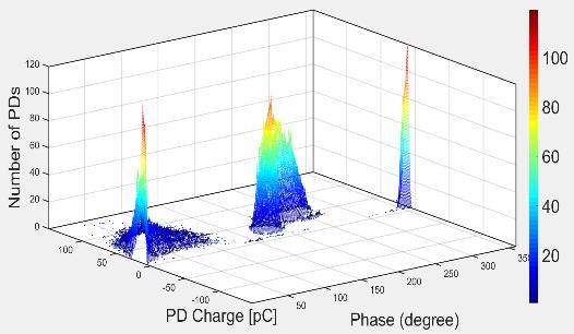
119 Comparison of results for Part 1 of test series 1, 2 and 3 at 1, 20 and 60 bar, respectively: 1 bar 20 bar 60 bar 102

120 From the previous comparison of results of the Part 1 of each test (this part includes the electric tree initiation stage and the growth till 50 % needle to plane electrode distance) it has been deduced that as the pressure increases the phase of occurrence of the PD pulses do not changes with pressure. However, the number of pulses occurring around a certain phase value, do change. As the pressure applied increases, the pulses tend to concentrate around the rising part of the voltage towards the maximum negative peak of the negative half side of the sinusoidal. At the same time, the high number of pulses occurring at lower pressures in the rising part of the voltage close to the maximum positive peak of the positive half side of the sinusoidal, as the pressure increases, these events keep occurring in the same part of the sinusoidal but in less number since many pulses have migrated their location to the negative half side of the voltage waveform. Therefore, as a consequence, if the pressure is increased the number of pulses occurring in the mentioned part of the negative half side, will increase. As mentioned in previous chapters, when the pressure increases the applied voltage increases and then, observing the voltage difference scatter plots for consecutive discharges it has been seen that as the applied pressure increases, the voltage difference maximum values increase and the data groups tend to be better defined. In other words, the scattering of data is smaller at higher pressure. This may be due to the higher pressure inside the tree channels and the consequent smaller volume of these as the tree develops. Finally, it has been seen how the electric tree tends to be, at lower pressures, more similar in shape to a typical bush type tree, whereas at higher pressures it tends to be more similar to a branch type tree. 103

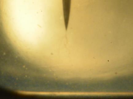
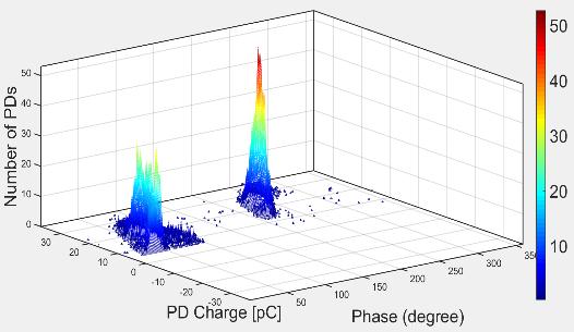
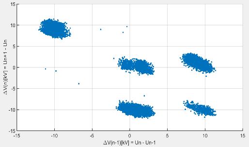
121 Comparison of results for Part 2 of test series 1, 2 and 3 at 1, 20 and 60 bar, respectively: 1 bar 20 bar 60 bar 104

122 From the previous comparison of results of the Part 2 of each test (part based on the pressure increasing till the PD reach the considered noise level) like in the Part 1 comparison of results, it has been appreciated that as the pressure increases the phase of occurrence of the PD pulses do not changes with pressure and the number of pulses occurring around a certain phase value, do change. As the pressure increases, the pulses tend again to concentrate around the rising part of the voltage towards the maximum negative peak of the negative half side of the sinusoidal. At the same time, it has been again appreciated that the high number of pulses occurring at lower pressures in the rising part of the voltage close to the maximum positive peak of the positive half side of the sinusoidal, as the pressure increases, these events keep occurring in the same part of the sinusoidal but in less number since many pulses have migrated their location, again, to the negative half side of the voltage waveform. Therefore, as a consequence, if the pressure is increased the number of pulses occurring in the mentioned part of the negative half side will increase. As have been seen in the previous Part 1, as the pressure increases the applied voltage increases and then, observing the voltage difference scatter plots for consecutive discharges it has been appreciated that as the applied pressure increases, the voltage difference maximum vales increase. However, since the same pressure process has been applied to all the samples during the Part 2 of each test, the same good definition of data groups can be seen in the three cases, regardless if the tree has been pre-grown at lower or higher pressure. Keeping that in mind, the only significant difference, as the pressure at which the tree has been pre-grown increases, is that the number of data groups decreases. This confirms the fact that trees pregrown at higher pressures will have smaller channels and then, less PD occurring points than trees pre-grown at lower pressures. These plots for the voltage difference have been compared with the ones obtained in the Part 1 of each test for the same samples and it has been observed that the scattering of the data points has been reduced, having the data groups better defined and keeping at the same time the same values of voltage differences. Finally, comparing the tree pictures from Part 1 and Part 2 comparisons it has been appreciated how the electric tree changes in a higher ratio when this one has been pre-grown at lower pressures. Trees pre-grown at the pressure of 60 bar generally do not change their shape but they sometimes tend to become more similar to bush type trees before growing in length. 105

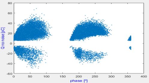
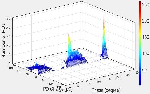
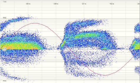
123 Comparison of results for Part 3 of test series 1, 2 and 3 at 1, 20 and 60 bar, respectively. 1 bar 20 bar 60 bar 106

124 From the previous comparison of results of the Part 3 of each test (part that includes the final growth of the tree till the end of the pre-breakdown stage), it has been appreciated that as seen in the Part 1 and 2 comparisons of results, as the pressure increases the phase of occurrence of the PD pulses do not changes with pressure and again the number of pulses occurring around a certain phase value, do change. In this last Part 3 comparison the pattern for the polarity of the occurring PD pulses is directly related with the previous Part 1 and Part 2 comparisons. However, if this one is just compared with Part 2 comparison, a clear phenomenon has been detected: when all the samples are subjected to the same pressure conditions, as done in Part 2, the increase of negative pulses at higher pressures than the one at which the tree has been pre-grown, is higher but not very different than the increase in positive pulses. However, in test parts like 1 and 3 where the pressure conditions applied are not the same in all samples, this increasing in number of negative pulses is significant if trees pre-grown at higher pressure are compared with those pre-grown at lower pressure. Therefore, pressure increasing generates more number of negative pulses and in general with higher magnitude of PD charge. Finally, comparing the tree pictures from Part 3 comparison it has been again confirmed that trees grown at lower pressures in SiR will have, normally, a bush type tree shape and those grown at higher pressure will have a branch type tree shape. In addition to the previous three comparisons, the following graphs representing the mean charge, maximum charge and average number of PD pulses per voltage cycle, have been presented for determining the type of electrical tree cavities formed in SiR by comparing these graphs with the PD patterns obtained from the OMICRON and the PhD thesis written by Hazlee A. Illias [35], where typical PD patterns are shown for distinct types of void shapes. First of all, it has been considered that different PD patterns have been appreciated by Hazlee A. Illias [35] as the diameter of a certain hemispherical cavity changes. He has concluded that for larger cavities, the maximum and minimum charge magnitudes are bigger than for smaller cavities. He has also explained the fact that for large spherical cavities, the number of PD pulses per cycle is smaller than for smaller spherical cavities. However, for large cylindrical cavities, the number of PD s per cycle has been explained to be higher than for small 107

125 cylindrical cavities. This opposite behaviour in cavity shapes has been used in this thesis to determine if the shape of the cavity generated, when the electric tree grows, is spherical or cylindrical knowing that the PD patterns obtained are characteristics from voids (see explanation for Graph 2 in MATLAB code for PSA results presentation and analysis, from data transformed from OMICRON PD measurements part). Just considering the PD patterns obtained from the OMICRON device for the 6 samples at 3 different pressure levels with three testing parts per sample (a total of 18 PD patterns), has not been enough to determine the shape of the cavity in SiR. For this reason, the following graphs have been used: Figure 79. Average number of PD s per voltage cycle in function of applied pressure for the three testing parts for each sample and for the first three tested samples 108

126 Figure 80. Maximum positive charge in function of applied pressure for the three testing parts for each sample and for the first three tested samples Figure 81. Maximum negative charge in function of applied pressure for the three testing parts for each sample and for the first three tested samples 109

127 Figure 82.Average positive charge in function of applied pressure for the three testing parts for each sample and for the first three tested samples gure 83. Average negative charge in function of applied pressure for the three testing parts for each sample and for the first three tested samples Fi After observing the previous graphs, it has been concluded that as the pressure increases the average number of PD pulses per voltage cycle increases for all the testing parts. In addition, as the pressure applied increases, the maximum positive and negative charge magnitude has increased in all the testing parts (the data point from the Part 1 at 60 bar has been neglected because the pattern is confirmed by the last three samples tested). On the contrary, as the pressure increases the mean positive and negative charge magnitude have decreased. 110

128 Finally, comparing these results with the results commented before from Hazlee A. Illias [35], it has been confirmed, firstly, that as the pressure increases, the size of the cavities will be smaller due to a decrease in mean charge magnitudes at higher pressures. Secondly, considering on the one hand that for large cylindrical cavities the number of PD s per cycle is expected to be higher than for small cylindrical cavities. And on the other hand, that the number of PD s per cycle in large spherical cavities is supposed to be smaller than for small spherical cavities. If it has been obtained that at higher pressures we have higher number of PD s per cycle (see Figure 79) and that the cavities have been confirmed to be smaller, spherical shaped cavities are confirmed as the void shape generated when the electric tree is grown in SiR. The typically obtained PD pattern in this thesis from the electric tree growth matches the pattern of a spherical, cylindrical and disc shaped cavities. However, the PSA in combination with the bibliographic research, has demonstrated that spherical cavities, decreasing in diameter as pressure increases, are the most probable generated void shape in SiR trees. 111

129 Chapter 5 Conclusions In this concluding chapter, all the conclusions obtained in this thesis have been put together at the same time that the validity of the hypotheses postulated in Hypothesis part has been discussed. The conclusions have been organized in the following points: The use of the NIKON camera model D7100 attached to a long-distance microscope lens, has been proved to be suitable for the proper observation of electrical tree growth in SiR samples inside a pressure vessel. Oil-saturated samples are not recommended to be tested under the explained setup conditions because of the elevated risk of breakdown occurrence due to the higher PDIV characteristic of this kind of samples. Regardless of the pressure conditions, the range of phase values of occurrence of PD coming from electric trees in SiR, are 0º to 110º and 170º to 280º. In addition, the negative half cycle of the sinusoidal voltage will generally have a bigger range of phase values of occurrence of PD, than the positive half cycle. The PSA result for the voltage difference between consecutive PD s (previously presented Graph 2), is recommended to be considered when the visualization of the number of light emission inception point in the electric tree is achieved. The differences in the number of groups of data in this graph, for the different stages of the electric tree, are thought to be directly related with the number of light emission inception points. In the initiation stage of the electric tree in SiR, PD pulses will occur more frequently, with less time difference between them and with a more progressive polarity change between pulses. On the contrary, for the intermediate and final stages, the consecutive PD events occur with less frequency but with a higher or more direct polarity change. 112

130 Nevertheless, the effect of the OMICRON sampling rate in this matter, is recommended to be checked in further works. PSA confirms that polarity changes between consecutive pulses occur in all the cases. Therefore, space charge dependency on the polarity change behaviour has been confirmed in all stages of the electric tree. Small time differences of 0.2 to 3 ms are characteristics from consecutive pulses with no polarity change. High time differences of 4 to 70 ms are characteristics from consecutive pulses with polarity change. As the applied pressure increases, sequential PD pulses, with high time difference between them, occur more often. The growth speed of the electric tree at the initiation stage, is higher when the pressure applied and therefore, the PDIV, are higher. The growth speed during the initiation stage is the highest for all the pressure values but the last one of 60 bar, where the trend changes and the pre-breakdown stage would have a higher growth speed. The use of the CCD camera model QuantEM:512SC from Photometrics, attached to the same long-distance microscope lens used for the NIKON camera, has shown to be suitable for the detection of light emission from the inside of a pressure vessel while the electric tree in SiR is perfectly visible. It has been concluded that changes need to be made in the setup for achieving the light emission from the electric tree (e.g. cover the internal surface of the pressure vessel with some material that do not allows light reflection). The phase of occurrence of PD pulses has been concluded to be independent from pressure but the number of events is not. As pressure increases, more pulses will appear in the negative half cycle of the sinusoidal voltage. In addition, the high number of pulses occurring in the positive half cycle at lower pressures, at higher pressures will migrate to the negative polarity or increase in number but in a lower ratio than the ones in the negative polarity side. 113

131 As a consequence of the previous affirmations, it has been confirmed that electrical trees in SiR pre-grown at higher pressures will have smaller channels and less PD occurring points than those pre-grown at lower pressures. Under the same pressurising process, electrical trees pre-grown at lower pressure will collapse faster than electrical trees pre-grown at higher pressures. The increase of applied pressure and therefore, the increase of the applied voltage due to higher PDIV, generates higher number of pulses, as mentioned before, but in addition, these pulses will have a higher charge magnitude. Finally, it has been concluded that the measured PD patterns generated as the electrical tree in SiR grows, are characteristic from void faults in the insulation material. The volume of this voids has been confirmed to be smaller as the pressure increases. In addition, it has been concluded that these voids will have a spherical shape. All the questions formulated in the Hypotheses part have been answered, except for those related with light emittance characteristics from the electric tree. 114

132 Chapter 6 Further work Since more results are to be known about the light emission characteristics of the electrical tree in SiR with dependency on the applied hydrostatic pressure, further work is suggested in this matter. Considering the theory explained in this thesis in the 2.4. Light emission in polymeric materials. Electroluminescence (EL) part, it is recommended to continue studying the differentiation of light emittance behaviour between different stages of the electrical tree growth while different pressure levels are applied. Since there is a considerable space charge dependency, specially at the needle-dielectric interface, it is suggested to study the affectation on the electrical tree initiation stage for different lengths of needle tip radius. Comparison of the PSA and the electric tree light emission, on the basis of the same PSA performed in this thesis, is recommended to fully understand the relation between different electrical tree PD patterns and the behaviour of the light emittance. Finally, it has been found important to highlight the possibility of making the same kind of samples used in this thesis, but filled with SiR material modified by the inclusion of nanofillers (as explained in 2.4. Light emission in polymeric materials. Electroluminescence (EL) part) or by directly trying other polymeric materials that could have similar properties as the SiR and that could be also used as insulation materials for subsea connectors. 115

133 Bibliography [1]. R. Leighton; R. D. Naybour; L. Warren, Light emission and electrical tree initiation in highly stressed XLPE and the effect of DC prestressing. In: Conduction and Breakdown in Solid Dielectrics, ICSD '98. Proceedings of the 1998 IEEE 6th International Conference on. Year: Pages: [2]. Yuan-Shing Liu, Takehiko Mizuno, Koichi Yasuoka and Shozo Ishii. Light Emission before and during Pre-breakdown on Polytetrafluoroethylene Surface with Metallized Electrodes under AC Voltage Application in Vacuum. In: Japanese Journal of Applied Physics, Volume 37, Part 1, Number 1. Year: Pages [3]. S. S. Bamji; A. T. Bulinski; R. J. Densley. Light emission from LDPE during electrical tree initiation. In: 1984 IEEE International Conference on Eletrical Insulation. Year: Pages: [4]. De Min Tu; Kwan C. Kao. Effects of hydrostatic pressure on water treeing properties of polyethylene. In: Conference on Electrical Insulation & Dielectric Phenomena - Annual Report Year: Pages: [5]. Toshikatsu Tanaka; Kanan Yokoyama; Yoshimichi Ohki; Yoshinao Murata; Yoitsu Sekiguchi; Manabu Goshowaki. High field light emission in LDPE/MgO nanocomposite. In: 2008 International Symposium on Electrical Insulating Materials (ISEIM 2008). Year: Pages: [6]. Jorunn Hølto and Erling Ildstad. Comparison of Electrical Treeing in Polypropylene and Cross linked Polyethylene. Norwegian University if Science and Technology. [7]. R. Vogelsang; B. Fruth; T. Farr; K. Fröhlich; Detection of electrical tree propagation by partial discharge measurements. In: European Transactions on Electrical Power, Volume 15, Issue 3. Year: Pages:

134 [8]. M. D. Noskov, M. Sack, A. S. Malinovski and A. J. Schwab. Measurement and simulation of electrical tree growth and partial discharge activity in epoxy resin. In: Journal of Physics D: Applied Physics, Volume 34, Number 9. Year: [9]. J V Champion, S J Dodd and G C Stevens. Quantitative measurement of light emission during the early stages of electrical breakdown in epoxy and unsaturated polyester resins. In: Journal of Physiscs D: Applied Physics, Volume 26, Number 5: Year: Pages: [10]. Mona Ghassemi; Mattewos B. Tefferi; Qin Chen; Yang Cao. Modeling a Liquid-Solid Insulation System Used in a DC Wet-Mate Connector. In: 2016 IEEE Conference on Electrical Insulation and Dielectric Phenomena (CEIDP). Year: Pages: [11]. DNV-GL STANDARD. DNVGL-ST Subsea power cables for wind power plants. Edition June [12]. Andreas Sumper. Hybrid AC-DC Offshore Wind Power Plant Topology: Optimal Design. In: IEEE Transactions on Power Systems. Year: 2015, Volume: 30, Issue: 4. Pages: [13]. Global Marine Offshore Renewables. [ONLINE] Available at: [Accessed 14 March 2017]. [14]. GCube Offshore Cable Claims Severity Increases by 25 % in [ONLINE] Available at: [Accessed 5 March 2017] [25] [15]. Hermanto Ang; Tore Markeset; Tor Ole Bang-Steinsvik. Condition Monitoring and Identification of Failure Modes of Subsea Electrical Equipments. In: 2013 Proceedings Annual Reliability and Maintainability Symposium (RAMS). Year: Pages:

135 [16]. Antônio P. C. Magalhães; João P. L. Salvador; Antonio C. S. Lima; M. Teresa Correia de Barros. Identification of incipient faults in subsea HVDC systems In: 2016 Power Systems Computation Conference (PSCC). Year: Pages: 1 7 [17]. Ingvild Spurkeland. Elektrisk trevekst og partielle utladninger i silikongummi for HVAC konnektorer. MSc Thesis. Norwegian University if Science and Technology. Year: [18]. Dimitros Panagiotopulos. AC Electrical Breakdown Strength of Solis Solid Interfaces. MSc Thesis. Norwegian University if Science and Technology. Year: [19]. Jon Thore Myklatun. Condition Monitoring of Subsea Connectors. MSc Thesis. Norwegian University if Science and Technology. Year: [20]. Rune Gravaune. Elektrisk trevekst i isolasjonsmaterialer for høyspente AC konnektorer. Norwegian University if Science and Technology. Year: [21]. B. X. Du; Z. L. Ma; Y. Gao. Phenomena and Mechanism of Electrical Tree in Silicone Rubber. In: 2009 IEEE 9th International Conference on the Properties and Applications of Dielectric Materials. Year: Pages: [22]. WACKER ELASTOSIL. ELASTOSIL LR3003/60 A/B Liquid Silicone Rubber. Technical data sheet for ELASTOSIL LR 3003/60 A/B / Version: 1.17 / Date of last alteration: [23]. WACKER ELASTOSIL. ELASTOSIL. The grades and properties of ELASTOSIL LR liquid silicone rubber. Brochure. [24]. Shin-Etsu Silicone. Characteristic properties of silicone rubber compounds. Edited version of the product data. Year: [25]. INMR Material & Design Requirements for MV Cable Accessories. [ONLINE] Available at: [Accessed 18 April 2017]. 118

136 [26]. F.H. Kreuger, Industrial High Voltage. Coordinating, Measuring, Testing. Delft Univeristy Press. 1 st Edition [27]. Mohamad Ghaffarian Niasar. Partial Discharge Signatures of Defects in Insulation Systems Consisting of Oil and Oil-impregnated Paper. Licentiate Thesis. Division of Electromagnetic Engineering. Stockholm, Sweden. KTH School of Electrical Engineering. Year:2012 [28]. Hosier, I L, Freebody, N A, Vaughan, A S, Swingler, S G and Moss, G (2011) Electrical Treeing in Silicone Rubber At 17th International Symposium on High Voltage Engineering, Germany Aug [29]. K. Urano; Y. Ehara; H. Kishida; T. Ito. Analysis of partial discharge phenomena by discharge magnitude and discharge luminesc ence in each phase angle. In:Proceedings of 1995 International Symposium on Electrical Insulating Materials. Year: Pages: [30]. Rainer Patsch and Farhad Berton. Pulse Sequence Analysis - a diagnostic tool based on the physics behind partial discharges. In: Journal of Physics D: Applied Physics, Volume 35, Number 1. Published 11 December Pages: [31]. Hasan Reza Mirzaei; Asghar Akbari; Mahdi Allahbakhshi; Mohammead Kharezi. New Attempts in Automated Partial Discharge Identification Using Pulse Sequence Analysis. In: 2009 IEEE 9th International Conference on the Properties and Applications of Dielectric Materials. Year: Pages: [32]. Y. Z. Arief; R. Patsch; D. Benzerouk; J. Menzel. Partial discharge characteristics in polyethylene using Pulse Shape and Pulse Sequence Analysis. In: 2007 International Power Engineering Conference (IPEC 2007). Year: Pages: [33]. Gorur G. Raju. Dielectrics in Electric Fields. Marcel Dekker. 1 st Edition

137 [34]. M. Hoof; R. Patsch. Pulse-Sequence Analysis : a new method for investigating the physics of PD-induced ageing In: IEE Proceedings - Science, Measurement and Technology. Year: 1995, Volume: 142, Issue: 1. Pages: [35]. Hazlee Azil Illias. Measurement and Simulation of Partial Discharges within a Spherical Cavity in a Solid Dielectric Material. PhD thesis. Faculty of Physical and Applied Science. School of Electronics and Computer Science. Universitiy of Southampton. Year:

138 Annex A. Trend line equation for the DAQ of the pressure sensor In order to calibrate the pressure sensor for obtaining the most accurate monitoring of the real-time pressure level inside the pressure vessel during a test, the following equation has been considered. This first order equation defines the gain (m) and offset (b) that the pressure sensor has to consider for displaying the real pressure value applied in each test. If this equation is transformed to our conditions, it becomes: Where P is the real pressure applied and I is the current output value given by the sensor in response to applied pressure. Therefore, a series of measurements have been taken by increasing the pressure by a 2bar interval every 2 minutes till reaching 100bar. A total of 50 data values of current and pressure have been obtained. With this data, a graph representing pressure against current has been plotted and a linear regression has been applied to the resulting data points. From the equation that defines that linear regression, the parameter m and b have been obtained and introduced as constants to the software that displays the pressure sensor measurements. Figure 84. Single-line electric scheme for the connection of the pressure sensor and the DAQ. 121

139 B. MATLAB codes B.1. MATLAB code for the reading of PD data from OMICRON streaming files % % % % % % % % % % % % % % % % % % % % % % % % % % % % % % % % % % % % % % % % % % % % % % % % % % % % % % % % % % % % % % % % % % % % % % % % %Reading of the PD data from OMICRON streaming generated files % % % % % % % % % % % % % % % % % % % % % % % % % % % % % % % % % % % % % % % % % % % % % % % % % % % % % % % % % % % % % % % % % % % % % % % % % % Clear all variables, windows and the screen before running program clear all; clc; close all; tic format long %folder = currentfolder name ; folder=2; %use rdefine frequency f=input('enter the frequency in Hz:'); %user define noise level for raw data noise=input ('Enter the noise level in pc, (example: 2.5): '); % Import Q data %define de folder number (e.g. 0002) [t_q1_1, q1_1]= importqdata('0002','unit2.1'); q1_1=q1_1*1e12; t_q1_1=t_q1_1*1000; % Import phase data %define de folder number (e.g. 0002) phase = importphdata('0002','unit2.1'); phase=phase*360; % Import voltage data %define de folder number (e.g. 0002) [tv1_1, v1_1] = importvdata('0002','unit2.1'); tv1_1=tv1_1*1000; % Changethe voltage offset in function of the settings in OMICRON %software (e.g ) offset_omicron=17.63; v1_1=(v1_1/1000)+offset_omicron; tv=tv1_1'; i=0; % Create matrix (aaa) with all needed raw data(charge time, charge, phase relation and occurring voltage) %qq=[t_q1_1,q1_1,phase]; noiseneg=-noise; length1=length(q1_1) for i=1:length1 if q1_1(i,1)>noise 122

140 end q(i,1)=q1_1(i,1); t(i,1)=t_q1_1(i,1); ph(i,1)=phase(i,1); end if q1_1(i,1)<(noiseneg) q(i,1)=q1_1(i,1); t(i,1)=t_q1_1(i,1); ph(i,1)=phase(i,1); end q_no_noise=q(q~=0); t_q1_1_no_noise=t(t~=0); phase_no_noise=ph(ph~=0); length2=length(q_no_noise); j=0; i=0; v=zeros(length2,1); for j=1:length2 for i=1:length(tv) if abs(t_q1_1_no_noise(j,1)-tv(i,1))<50e-3 v(j,1)=v1_1(i,1); end end end aa=[t_q1_1_no_noise,q_no_noise,phase_no_noise,v]; aaa=[t_q1_1_no_noise,q_no_noise,phase_no_noise]; % Plots for PD pattern without noise and PD histogram figure histogram(q1_1); set(gca,'ygrid','on','xgrid','on','linewidth',2,'fontsize',20) xlabel ('Q [pc]') ylabel ('Frequency') figure histogram(q_no_noise); set(gca,'ygrid','on','xgrid','on','linewidth',2,'fontsize',20) xlabel ('Q no noise [pc]') ylabel ('Frequency') % Deletes PDs that are assumed to be background noise from raw data j=0; jjj=0; jj=0; for j=1:length(q_no_noise) if q_no_noise(j)<0 jj=jj+1; q_no_noise_neg(jj,1)=q_no_noise(j); end if q_no_noise(j)>0 jjj=jjj+1; q_no_noise_pos(jjj,1)=q_no_noise(j); end end % Converts all PDs to positive ones keeping the order of occurence j=0; 123

141 jj=0; for j=1:length(q_no_noise) if q_no_noise(j)<0 jj=jj+1; q_no_noise_3d(jj,1)=(-1)*q_no_noise(j); end if q_no_noise(j)>0 jj=jj+1; q_no_noise_3d(jj,1)=q_no_noise(j); end end q_no_noise_neg_sortted=sort(q_no_noise_neg); q_no_noise_pos_sortted=sort(q_no_noise_pos); % Creates vector for number of PD occurring in every phase value interval %of 0.5º till 360º j=0; jj=0; jjj=0; uu=0; count=0; for j=0.5:0.5:360 uu=uu+1; for jj=1:length(phase_no_noise) if (jjj<phase_no_noise(jj))&&(phase_no_noise(jj)<j) count=count+1; end end jjj=jjj+0.5; events_phase(uu)=count; count=0; end % Clear counters clear ( 'Ip'); clear ( 'In'); clear ( 'qqn'); clear ( 'qqp'); % Calculations of statistics % ============================================= %time recorded total_time=max(aaa(:,1)); disp('total time recorded') disp(total_time) % number of cycles number_of_cycles=total_time*f; disp('total number of cycles') disp (number_of_cycles) %noise level disp('noise level') disp(noise) %sum of positive charge Qptot=sum(q_no_noise_pos(:,1)); disp('sum of positive charge') disp(qptot) 124

142 %sum of negative charge Qntot=sum(q_no_noise_neg(:,1)); disp ('sum of negative charge') disp(qntot) %sum of charge Qtot=Qptot+Qntot; %number of PD s registered number_of_pd_no_noise=numel(q_no_noise(:,1)); disp('number of PD registered (without noise)') disp(number_of_pd_no_noise) %number of positive PD s registered number_of_pd pos_no_noise=numel(q_no_noise_pos(:,1)); disp('number of positive PD (without noise)') disp(number_of_pd pos_no_noise) %number of negative PD s registered number_of_pd_neg_no_noise=numel(q_no_noise_neg(:,1)); disp('number of negative PD (without noise)') disp(number_of_pd_neg_no_noise) %mean positive charge q_average_pos=qptot/number_of_pd pos_no_noise ; disp('mean positive charge') disp(q_average_pos) %mean negative charge q_average_neg=qntot/number_of_pd_neg_no_noise ; disp('mean negative charge') disp(q_average_neg) %mean charge average_overall_charge=qtot/number_of_pd_no_noise ; disp('mean overall charge') disp(average_overall_charge) %PDs per cycle PD_per_cycle=number_of_PD_no_noise/number_of_cycles ; disp('number of PD per cycle') disp(pd_per_cycle) %max positive charge calculated from top 1 % qmax_pos=max(q_no_noise_pos(:,1)); disp('maximum charge recorded') disp(qmax_pos) %max negative charge calculated from bottom 1 % qmax_neg=min(q_no_noise_neg(:,1)); disp('minimum charge recorded') disp(qmax_neg) j=0; cycle_number=zeros(length(t_q1_1_no_noise),1); for j=1:length(t_q1_1_no_noise) cycle_number(j,1)=t_q1_1_no_noise(j,1)*f; end 125

143 aaaa=[t_q1_1_no_noise,q_no_noise,phase_no_noise,v,cycle_number]; savefile='data export.txt'; save(savefile,'total_time','number_of_cycles','noise','qptot',... 'Qntot','number_of_PD_no_noise','number_of_PD pos_no_noise','number_of_pd_ neg_no_noise',... 'q_average_pos','q_average_neg','average_overall_charge','pd_per_cycle',... 'qmax_pos','qmax_neg','-ascii','aaaa'); %[s,msg]=replaceinfile('.',',','data export.txt'); savefile='chargedata.mat'; save(savefile,'aa','-ascii'); % Create figure figure1=figure; % Create axis axis1=axis('parent',figure1,'ytick',... [-4e09-2e09 0 2e09 4e09],'YGrid','on',... 'YColor',[0 0 1],'XGrid','on'); % Uncomment the following line to preserve the X limits of the axis xlim(axis1,[0 360]); % Create plot semilogy(phase_no_noise,q_no_noise,'parent',axis1,'markersize',3,'marker',' x','linestyle','none','displayname','pd_activity'); % Create y label ylabel('q no noise [pc]','color',[0 0 1]); xlabel('phase [º]','Color',[0 0 1]); % Create figure figure2=figure; % Create axis axis2=axis('parent',figure2,'ytick',... [-4e09-2e09 0 2e09 4e09],'YGrid','on',... 'YColor',[0 0 1],'XGrid','on'); % Uncomment the following line to preserve the X limits of the axis xlim(axis2,[0 360]); % Create plot plot(phase,q1_1,'parent',axis2,'markersize',3,'marker',... 'x','linestyle','none','displayname','pd_activity'); % Create y label ylabel('q [pc]','color',[0 0 1]); xlabel('phase [º]','Color',[0 0 1]); % Create figure figure3=figure; % Create axis 126

144 axis3=axis('parent',figure3,'ytick',... [-4e09-2e09 0 2e09 4e09],'YGrid','on',... 'YColor',[0 0 1],'XGrid','on'); % Uncomment the following line to preserve the X limits of the axis xlim(axis3,[0 360]); % Create plot plot(phase_no_noise,q_no_noise,'parent',axis3,'markersize',3,'marker',... 'x','linestyle','none','displayname','pd_activity'); % Create y label ylabel('q no noise [pc]','color',[0 0 1]); xlabel('phase [º]','Color',[0 0 1]); % Create figure figure4=figure; % Create axis axis4=axis('parent',figure4,'ytick',... [-4e09-2e09 0 2e09 4e09],'YGrid','on',... 'YColor',[0 0 1],'XGrid','on'); % Create plot plot(tv,v1_1,'parent',axis4) % Create y label ylabel('voltage [kv]','color',[0 0 1]); xlabel('time [ms]','color',[0 0 1]); %Define max charge recorded if qmax_pos>abs(qmax_neg) qmax=round(qmax_pos); else qmax=round(abs(qmax_neg)); end % Generation of the 3D plot for PD value vs phase vs Number of PDs width=200; height=200; chargedisp=('pc'); CasPhasePD2=zeros(width,width); for PDm = 1:length(phase_no_noise) phi2 = round(phase_no_noise(pdm,1)/360*width); if phi2 > width phi2 == 0 phi2 = width; end cas2 = round((abs(q_no_noise_3d(pdm,1))+qmax)/qmax*height/2); end if cas2 == 0 cas2 = cas2+1; end CasPhasePD2(cas2,phi2) = CasPhasePD2(cas2,phi2)+1; [XX,YY]=meshgrid(1:1:height,1:1:width); figure 127

145 contour3(xx/width*360,(yy-height/2)/(height/2)*qmax,casphasepd2,200) %contour3(xx,yy,casphasepd2,200) box on set(gca,'ygrid','on','xgrid','on','linewidth',2,'fontsize',20) colormap(jet); shading interp colorbar('location','eastoutside','fontsize',36,'fontname','arial') xlabel('phase (degree)','fontsize',36,'fontname','arial') ylabel('pd Charge [pc]','fontsize',36,'fontname','arial','horizontalalignment','left'); zlabel('number of PDs','FontSize',36,'FontName','Arial') grid on axis on toc B.2. MATLAB code for the PSA generation % % % % % % % % % % % % % % % % % % % % % % % % % % % % % % % % % % % % % % % % % %Pulse Sequence Analyisis (PSA) % % % % % % % % % % % % % % % % % % % % % % % % % % % % % % % % % % % % % % % % % % % Clear all variables,windows and the screen before running program clear all; clc; close all; tic % Decimal format format long % Defining matrix of inputdata [time,pd,phase,v,cycle_number]=textread('data export.txt',' %f %f %f %f %f','headerlines',14); % Bar graph with phase values of PD events sortted figure(1) bar(sort(phase),0.4) set(gca,'ygrid','on','xgrid','on','linewidth',2,'fontsize',20) xlabel ('Phase values sortted') ylabel ('Phase at which PD occurs[º]') % Define Voltage diference between consecutive PDs lengdexy=length(time)-2; xy =zeros(lengdexy,2); i=0; cyc_number=zeros(lengdexy,1); for i=1:lengdexy xy(i,1)=v(i+1)-v(i); xy(i,2)=v(i+2)-v(i+1); cyc_number(i,1)=cycle_number(i,1); end x1=xy(:,1); y1=xy(:,2); % Plots for voltage difference figure (2) 128

146 scatter(x1,y1,'fill') set(gca,'ygrid','on','xgrid','on','linewidth',2,'fontsize',20) xlabel ('\DeltaV(n-1)[kV] = Un - Un-1') ylabel ('\DeltaV(n)[kV] = Un+1 - Un') figure (3) plot(x1,y1) set(gca,'ygrid','on','xgrid','on','linewidth',2,'fontsize',20) xlabel ('\DeltaV(n-1)[kV] = Un - Un-1') ylabel ('\DeltaV(n)[kV] = Un+1 - Un') figure(4) histogram(x1) set(gca,'ygrid','on','xgrid','on','linewidth',2,'fontsize',20) xlabel ('\DeltaV(n-1)[kV] = Un - Un-1') ylabel ('Frequency') figure(5) bar(sort(x1),0.4) set(gca,'ygrid','on','xgrid','on','linewidth',2,'fontsize',20) xlabel ('\DeltaV(n-1)values sorted') ylabel ('\DeltaV(n-1)[kV]') figure (6) scatter(cyc_number,y1,'fill') set(gca,'ygrid','on','xgrid','on','linewidth',2,'fontsize',20) xlabel ('voltage cycle number') ylabel ('\DeltaV(n-1)[kV] = Un - Un-1') % Re-read the matrix of input data [time,pd,phase,v,cycle_number]=textread('data export.txt',' %f %f %f %f %f','headerlines',14); % Define Tmie diference between consecutive PDs lengdexy=length(time)-2; xy=zeros(lengdexy,2); i=0; for i=1:lengdexy xy(i,1)=time(i+1)-time(i); xy(i,2)=time(i+2)-time(i+1); volt(i,1)=v(i); end x2=xy(:,1); y2=xy(:,2); % Plots for time difference figure(7) scatter(x2,y2,'fill') set(gca,'ygrid','on','xgrid','on','linewidth',2,'fontsize',20) xlabel ('\Deltat(n-1)[ms]') ylabel ('\Deltat(n)[ms]') figure(8) histogram(x2) set(gca,'ygrid','on','xgrid','on','linewidth',2,'fontsize',20) xlabel ('\Deltat(n-1)[ms]') ylabel ('Frequency') 129

147 figure(9) bar(sort(x2),0.4) set(gca,'ygrid','on','xgrid','on','linewidth',2,'fontsize',20) xlabel ('\Deltat(n-1)values sorted') ylabel ('\Deltat(n-1)[ms]') % Plots for voltage difference and time difference vs PD voltage of occurence figure(10) scatter(volt,y2,'fill') set(gca,'ygrid','on','xgrid','on','linewidth',2,'fontsize',20) xlabel ('U at which each PD occurs [kv]') ylabel ('\Deltat(n+1)[ms]') figure(11) plot(volt,y2) set(gca,'ygrid','on','xgrid','on','linewidth',2,'fontsize',20) xlabel ('U at which each PD occurs [kv]') ylabel ('\Deltat(n+1)[ms]') figure(12) scatter(volt,x1,'fill') set(gca,'ygrid','on','xgrid','on','linewidth',2,'fontsize',20) xlabel ('U at which each PD occurs [kv]') ylabel ('\DeltaV(n-1)[kV]') figure(13) plot(volt,x1) set(gca,'ygrid','on','xgrid','on','linewidth',2,'fontsize',20) xlabel ('U at which each PD occurs [kv]') ylabel ('\DeltaV(n-1)[ms]') % Defining ratio between voltage difference and time difference % between consecutive PD events i=0; for i=1:lengdexy x3(i,1)=(x1(i))/(x2(i)); y3(i,1)=(y1(i))/(y2(i)); end % Plots for ratio between voltage difference and time difference % between consecutive PD events figure(14) scatter(x3,y3,'fill') set(gca,'ygrid','on','xgrid','on','linewidth',2,'fontsize',20) xlabel ('\DeltaV(n-1)[kV] / \Deltat (n-1) [ms]') ylabel ('\DeltaV(n)[kV] / \Deltat (n) [ms]') % Hostrogram for phase of occurence of PD events figure(15) histogram(phase) set(gca,'ygrid','on','xgrid','on','linewidth',2,'fontsize',20) xlabel ('Phase[º]') ylabel ('Frequency') % Histogram for time of occurence figure(16) histogram(time) set(gca,'ygrid','on','xgrid','on','linewidth',2,'fontsize',20) xlabel ('Time[ms]') 130

148 ylabel ('Frequency') C. NIKON camera settings for long exposure times, in dark conditions with the long-distance microscope lens A list of settings that have been changed in the NIKON camera, for the proper observability of the electrical tree light emission, has been described in this part. Taking into account that the pictures have been taken being the camera attached to a long-distance microscope, the main settings changed are: 1- Exposure time: the exposure time has been set to BULB mode so it can be controlled every time a picture is taken. This mode combined with the remote-control mode (explained below), will allow the user the control the exposure time of each picture with no restriction to any predefined exposure time setting. In this modes combination, when the shutter release is initially pressed, the camera will open its mirror, then with a second press, the camera sensor will start its exposure time and with a final press, the mirror will close and exposure time will end. For a long exposure time, the real-time behaviour of the electric tree cannot be observed while the camera sensor is exposed. 2- Image quality: in order to obtain the highest resolution possible when processing the pictures in the PC, the image quality setting has been set to NEF(RAW)+JPEG fine, allowing the postprocessing of the RAW format pictures with an appropriate software at the same time that the JPEG format can be handled easily for quick picture preview. 3- Image area: since the area needed to be focused is relatively small compared with the total focus area of the lens, the image area setting has been set to 1.3x (18x12). 4- Remote-control mode: as mentioned before, the camera has been used while applying HV, therefore, this one is placed together with the lens, inside the HV cell. In order to take the pictures at the desired instant of the test, to keep all the security regulations 131

149 and to reduce the vibration generated by the mirror when a picture is taken, the remote-control mode setting has been set to Mirror UP (Mup). Combined with the exposure time settings (above), this remote-control mode reduces the vibration generated when the mirror is removed an instant before the camera sensor begins to be exposed. Therefore, this mode allows the user to push the remote control, firstly, to open the mirror, and after waiting a few seconds (2 sec), to push again the control to start the exposure time. The result will be a long-exposed picture with a considerable noise reduction. 5- Remote on duration: due to the fact that the tests could last for a relatively long time (up to 1hour), the time setting that would deactivate the remote-control mode if that one is not used, is set to the maximum value of 15 min. This means that at least on picture must be taken before 15 minutes after the previous picture. 6- White Balance (WB): the incident light to the sample, when the test is performed, slightly changes every time a new sample is introduced into the pressure vessel. Then, in order to appreciate, in every case, the electric tree during the live view and in the pictures taken, the white balance setting is changed to AUTO. 7- ISO: the amount of incident light to the sample is relatively low. Then, for our conditions, and the lowest ISO setting available (ISO 100), has been used. It is wise not to keep the ISO settings at high values because the noise generated in every picture will increase. Therefore, ISO setting must be kept as low as possible in function of the available light in every case. 8- Aperture: since the long-distance microscope lens shutter aperture is manually controlled from a metallic tap, it is wise to keep these aperture to the maximum opening to let all the incoming light reach the camera sensor. 132

150 D. Complementary graphs from the results part Most of the results presented in the results part of this thesis, correspond to the tests 1, 2 and 3. In this section the resulting graphs from the tests 4,5 and 6 at 1, 20 and 60 bar respectively, are presented. Figure 85.Box plots for the PD phase of occurrence for each test case for the positive half side of the sinusoidal voltage (last three tested samples). Figure 86. Box plots for the PD phase of occurrence for each test case for the negative half side of the sinusoidal voltage (last three tested samples). 133

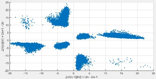
151 Comparison of results for Part 1 of test series 4, 5 and 6 (last three tested samples) at 1, 20 and 60 bar, respectively. 1 bar 20 bar 60 bar 134

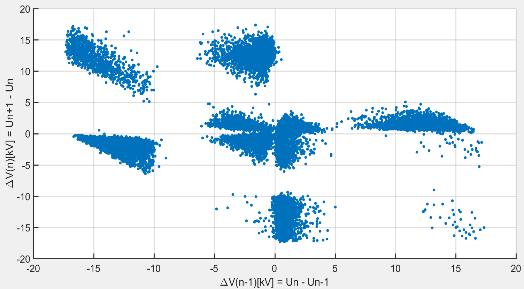
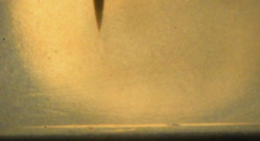
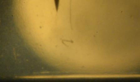
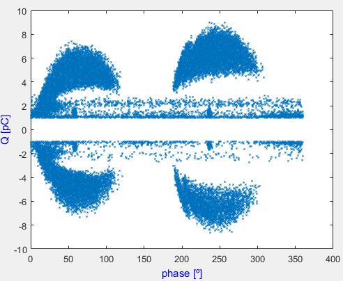
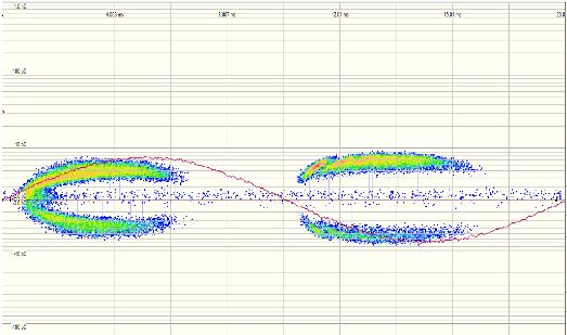
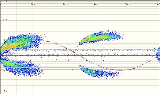
152 Comparison of results for Part 2 of test series 4, 5 and 6 (last three tested samples) at 1, 20 and 60 bar, respectively. 1 bar 20 bar 60 bar 135

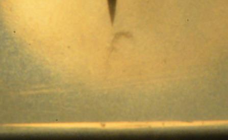
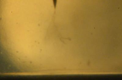
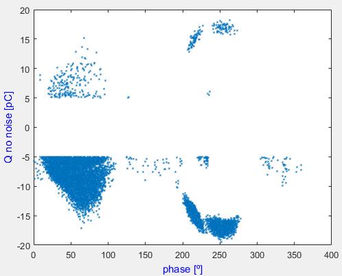
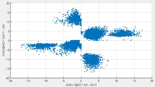
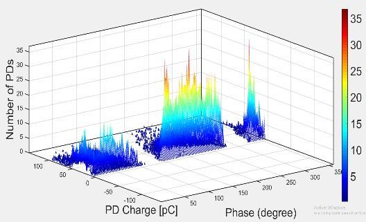
153 Comparison of results for Part 3 of test series 4, 5 and 6 (last three tested samples) at 1, 20 and 60 bar, respectively. 1 bar 20 bar 60 bar 136