UNCERTAINTY & SENSITIVITY ANALYSIS

Size: px

Start display at page:

Download "UNCERTAINTY & SENSITIVITY ANALYSIS"

Veronica Nicholson
6 years ago
Views:

1 October 24, 2016 SAL-Mathematical Computational Modeling Science Center, Arizona State University 1 UNCERTAINTY & SENSITIVITY ANALYSIS Saurabh Biswas Dheeraj Lokam Sustainability, ASU Computer Engineering, ASU Anuj Mubayi School of Human Evolution & Social Change, SAL-MCMSC

2 Outline Introduction of UA & SA Analysis Sampling Methods Uncertainty Methods Sensitivity Method (PRCC) Examples & simple codes Using Cluster to conduct experiments

3 Purpose of Uncertainty & Sensitivity Analyses 1. Evaluating the applicability of the model: understanding the behavior of the system being modeled. 2. Determining parameters for which it is important to have more accurate values and which can be left at default value. 3. Prioritize additional data collection. 4. Estimate potential errors in model forecasts that could be due to parameter value errors.

4 What is Uncertainty and Sensitivity Analysis? Uncertainty Analysis (UA) quantifies the uncertainty in the outcome of a model. How the uncertainty in the output of a model is related to different sources of uncertainty in the model input? Sensitivity Analysis (SA) has the complementary role of ordering by importance, the strength, and relevance of the inputs in determining the variation in the output. Measures the change in model output associated with the change (perturbation) in model input. Output variable space Y 0 Y k Model Sensitivity Index: SI ( Y ( P 0 0 Yk P k ) / Y0 ) / P 0 Input parameter space Min P 0 (Calibrated) P k (Perturbed) Max

5 SIR Infectious Disease Model: Kermack and McKendrick, 1927 S βs(i/n) I νi R S N di dt or = βi νi = ( β ν)i ( I(t) I(0)e β ν )t I(t) increases R 0 = β ν >1 Reproduction Number Establishment of a Critical Mass of Infectives! R o >1 implies growth while R o <1 extinction.

6 S β I ν R We have seen these two types of outcomes: If R 0 >1 If R 0 <1 Infectives in SIR model Infectives in SIR model Infectives Infectives Time (days) Time (days) This poses the questions: What determines whether an outbreak takes off? How large will the outbreak be? Proportion of population R 0 = R 0 =5 R 0 =3 R 0 =2 Time

7 Mathematical Model (consists of parameters) & Output (of interest) Mathematical Model z ' = f (z,θ) Θ = {θ 1,θ 2,...,θ n } Output Variable y = h(t;θ) Example Input Output SIR Mode with demography & disease mortality β, ν, µ, α R 0

8 General Sampling Based Global UA/SA Procedure Input Output θ 1 θ 2 Model: Z=f(Θ, Z) z 2 z 1 z3 Uncertainty Analysis θ n where, z=(z 1,z 2,z 3,z 4,z 5,,z k ) T & Θ=(θ 1, θ 2,.., θ n ) T z 4 z k z 5 Sensitivity Analysis STEPS: 1. Assigning distribution to the input parameters 2. Proper sampling from distribution of input parameters 3. Computing distribution of output variables using sample of input parameters in the Model 4. Quantifying uncertainty and sensitivity using samples of input and output variables

9 Methods UA methods: Quantitatively and qualitatively measuring variations: Histogram, Confidence/Credible Intervals, Box-Whisker Plot SA methods: Standardized Regression Coefficients Classification and Regression Trees Variance-based Sensitivity Methods Extended-Fourier Amplitude Sensitivity Test (efast) Partial Rank Correlation Coefficients (Primarily used)

10 Method of Sampling Monte Carlo sampling Random sampling from a distribution Each parameter is sampled from a probability distribution function (pdf) depending on what is known Latin hypercube sampling (LHS) A stratified method of sampling without replacement Divides by N equal probable intervals and then chooses one point from each interval Generate a matrix with N rows and θ columns (N sample size, θ number of varied parameters) LHS sampling can be done using commands in Matlab example lhsnorm, lhsdesign

11 Example Goals of UA/SA in Mathematical-Epidemiology Investigating the impact on model output, based on the changes in input parameters. Model output can be of two types: 1. Constant in time e.g. R 0 2. Function of time e.g. I(t) i.e., number of infected individuals at time t (sensitivity indexes are computed at each time here)

12 How to perform these analyses? I. Design the experiment: what are the input and output variables. II. III. IV. Assign pdf to each input variable. Generate an input matrix using all input variables through a appropriate sampling method. Evaluate the model, thus creating a distribution for output variable (Uncertainty analysis). V. Assess the influences or relative importance of each input variable on the output variable (Sensitivity analysis). VI. Repeat the steps to provide a measure of the stability of the results.

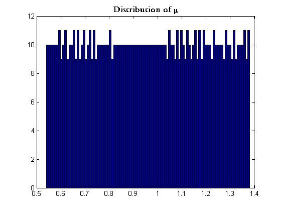
13 Example Results of UA Input: β, ν, µ, α Output: R 0 Model: Distribution of R 0

14 CRITICAL STEPS: Assigning distribution to the input parameters Computing distribution of output variables using sample of input parameters in the model (Uncertainty Analysis) Quantifying sensitivity using samples of input on output variables (Sensitivity Analysis)

15 EPIDEMIC MODEL with TREATMENT No need to redefine SIR categories, if biology suggests some other relevant factors. bn β S (I/N) S I µs µi µr δi R ν à per capita rate of treatment (per unit time) 1/ν à average time to treatment

16 II. Data for Initial Distribution Bhattacharyya J. & Hati A.K. The Adverse Affects of Kala-Azar (Visceral Leishmaniasis) in Women.In: The female client and the health-care provider, edited by Janet Hatcher Roberts and Carol Vlassoff. Ottawa, Canada, International Development Research Centre [IDRC], : Distribution of Time to Treatment Time to Treatment I. What are the input and output variables. II. Assign pdf to input variable. III. Sampling method. IV. Uncertainty analysis. V. Sensitivity analysis. VI. Repeat the steps.

17 CRITICAL STEPS: Assigning distribution to the input parameters Computing distribution of output variables using sample of input parameters in the model (Uncertainty Analysis) Quantifying sensitivity using samples of input on output variables (Sensitivity Analysis)

18 IV. Showing uncertainty Showing Distribution 25th Percentile Median Mean 75th Percentile Boxplot Summary Statistics: Mean, Variance, Minimum and Maximum Entropy of a Empirical Distribution: 1 n n k=1 p k log p k Consider the histogram having frequencies [f 1, f 2,.f n ] where 0<=f i <=1 for all i. Entropy of empirical distribution is H( f 1, f 2,..., f n ) = 1 n k=1 f k log f k If all data in one cell then H=0. If the histogram is uniform distributed (i.e. f i =1/n) then H=1. n I. What are the input and output variables. II. Assign pdf to input variable. III. Sampling method. IV. Uncertainty analysis. V. Sensitivity analysis. VI. Repeat the steps.

19 CRITICAL STEPS: Assigning distribution to the input parameters Computing distribution of output variables using sample of input parameters in the model (Uncertainty Analysis) Quantifying sensitivity using samples of input on output variables (Sensitivity Analysis)

20 V. Finding the Sensitivity Index: Partial rank correlation coefficient (PRCC) PRCC is a robust sensitivity measure for nonlinear but monotonic relationships between model parameters and model outputs. Computation involve following steps: III. Sampling Method: common for both UA & SA 1. Generate samples: a) LHS of input parameters (θ i ) from pre-assigned distribution b) Output parameter (Z) samples using LHS and output function 2. Rank transform both input and output data stored in the two matrices 3. For each input parameter θ, compute two linear regression models using the samples a) First: between Z and rest of the input parameters (leaving θ) b) Second: between θ and rest of the input parameters (leaving Z) 4. Compute correlation coefficient between the two residuals (actual value linear regression value) from the two regression lines 5. This Corr. Coeffs. are the PRCCs (lying between -1 and 1) referred sensitivity indexes in the analysis

21 1 a. Latin Hypercube Sampling (LHS) of Input Parameters Image taken from Marino et al Generate samples: a) LHS of input parameters (θ i ) from preassigned distribution b) Output parameter (Z) samples using LHS and output function 2. Rank transform both input and output data stored in the two matrices 3. For each input parameter θ, compute two linear regression models using the samples a) First: between Z and rest of the input parameters (leaving θ) b) Second: between θ and rest of the input parameters (leaving Z) 4. Compute correlation coefficient between the two residuals (actual value linear regression value) from the two regression lines 5. This Corr. Coeffs. are the PRCCs (lying between -1 and 1) referred sensitivity indexes in the analysis The sample size is stratified and divided in five (e.g., sample size) equal probability segments of the chosen distribution. A value is selected from each interval and then placed randomly.

22 1 b. Input / Output Samples Matrix Image taken from S. Marino et al Generate samples: a) LHS of input parameters (θ i ) from pre-assigned distribution b) Output parameter (Z) samples using LHS and output function 2. Rank transform both input and output data stored in the two matrices 3. For each input parameter θ, compute two linear regression models using the samples a) First: between Z and rest of the input parameters (leaving θ) b) Second: between θ and rest of the input parameters (leaving Z) 4. Compute correlation coefficient between the two residuals (actual value linear regression value) from the two regression lines 5. This Corr. Coeffs. are the PRCCs (lying between -1 and 1) referred sensitivity indexes in the analysis Each row of input matrix contains Z samples of one input parameter (θ). Output matrix contains Z samples of output function example R 0.

23 2. Rank Transform the Input / Output Matrices Image taken from Marino et al Generate samples: a) LHS of input parameters (θ i ) from preassigned distribution b) Output parameter (Z) samples using LHS and output function 2. Rank transform both input and output data stored in the two matrices 3. For each input parameter θ, compute two linear regression models using the samples a) First: between Z and rest of the input parameters (leaving θ) b) Second: between θ and rest of the input parameters (leaving Z) 4. Compute correlation coefficient between the two residuals (actual value linear regression value) from the two regression lines 5. This Corr. Coeffs. are the PRCCs (lying between -1 and 1) referred sensitivity indexes in the analysis Rank the matrix with values in the columns independently of the other columns in descending or ascending order

24 Example: Ranking of matrix columns Input Output Matrices are converted into their ranks

25 Partial Correlation Coefficients (PCC) A coefficient of correlation r between 2 r.v. is a quantitative index of association between these two variables. (if correlation is ± 1, the variables are strongly correlated; + sign indicates increasing relationship; - sign indicates decreasing relationship) Sampled points (X 1i, X 2i, X 3i, Y i ) for i=1,,n Partial correlation coefficient (PCC) is a measure of strength of the linear relationship between variables after controlling for the effects of the other variables PCC(Y, X 1 )=? Y^ How: Regression models: = β^ 1+ β^ 2 X 2 + β^ 3 X 3 & X^ 1 = ~ β 1+ ~ β 2 X 2 + ~ β 3 X 3 Residuals (Y Y^ ) and (X 1 X^ 1) represent what remains after variables X 2 & X 3 has explained all the variation it can in the variables Y and X 1 separately. r Y,X1 X 2,X 3 Then r Y,X1 X 2,X 3 = ry^ Y,X^ X i.e., PCC gives the strength of the correlation between Y and a given input X 1 after adjustment for any effect due to correlation between X 1 and any of the X 2 and X 3.

26 3. Example: Computing Linear Regression Models Compute two regressions using output (e.g., R 0 ) and each of the input (e.g., β, ν, µ, α) rank transformed data. Example: For each input parameter two linear regressions are obtained β = a 0 + a 1 ν + a 2 µ + a 3 α R 0β = b 0 + b 1 ν + b 2 µ + b 3 α (no R 0 in this regression) (no β in this regression) 1. Generate samples: a) LHS of input parameters (θ i ) from pre-assigned distribution b) Output parameter (Z) samples using LHS and output function 2. Rank transform both input and output data stored in the two matrices 3. For each input parameter θ, compute two linear regression models using the samples a) First: between Z and rest of the input parameters (leaving θ) b) Second: between θ and rest of the input parameters (leaving Z) 4. Compute correlation coefficient between the two residuals (actual value linear regression value) from the two regression lines 5. This Corr. Coeffs. are the PRCCs (lying between -1 and 1) referred sensitivity indexes in the analysis Residuals obtained from linear regression models are also noted Same steps are also carried out for ν, µ, α

27 Example: Final Table Containing Residuals β ν µ α R 0 β β-β R 0β R 0β - R 0β Residuals are in columns: β β & R 0 β R 0β

4. Correlation Coefficient Compute the correlation between the two residuals β β & R 0β R 0β as follows: r β = n n (β i β i )(R 0βi R 0βi ) i=1 (β i β i ) 2 (R 0βi R 0βi ) 2 i=1 Similarly compute

28 4. Correlation Coefficient Compute the correlation between the two residuals β β & R 0β R 0β as follows: r β = n n (β i β i )(R 0βi R 0βi ) i=1 (β i β i ) 2 (R 0βi R 0βi ) 2 i=1 Similarly compute other correlation coefficients à n i=1 r ν,r µ, r α 1. Generate samples: a) LHS of input parameters (θ i ) from pre-assigned distribution b) Output parameter (Z) samples using LHS and output function 2. Rank transform both input and output data stored in the two matrices 3. For each input parameter θ, compute two linear regression models using the samples a) First: between Z and rest of the input parameters (leaving θ) b) Second: between θ and rest of the input parameters (leaving Z) 4. Compute correlation coefficient between the two residuals (actual value linear regression value) from the two regression lines 5. This Corr. Coeffs. are the PRCCs (lying between -1 and 1) referred sensitivity indexes in the analysis

29 Example: Final Results Showing Sensitivity Index (PRCCs) in Tornado Plot We see: 1. β is highly correlated with R 0 as absolute value of its PRCC value is higher than corresponding value of other parameters 2. β is positively correlated with R 0

30 Simulations: 1. MATLAB Code to generate samples runs=1000; % size of the sample beta_lhs=lhsnorm(3.27,0.9,runs); % beta LHS sampling from normal pdf nu_lhs=lhsnorm(4.2,0.3,runs); % nu LHS sampling from normal pdf alpha_lhs=lhs_call(2.51,0.30,0.54,0.04,runs,'unif'); %Uniform distribution, %LHS_Call(xmin,xmean,xmax,xsd,nsample,distrib,threshold) mu_lhs=lhs_call(1.38,0.46,0.54,0.04,runs,'unif'); %Uniform distribution, %LHS Matrix L=[beta_LHS nu_lhs mu_lhs alpha_lhs]; y=[];% response R0=beta/(nu + mu + alpha) for i=1:size(l,1) y(i)=l(i,1)/(l(i,2)+l(i,3)+l(i,4)); end R0=y'; Code generates values for β, ν, μ, α and R 0

31 Simulations: 2. MATLAB code for ranking matrix function [r,i]=ranking(x) % [r,i]=ranking(x) % Ranking of a matrix % input: % x : vector (nrow,n columns) % output: % r : rank of the Matrix (nrow,n columns) % i : index vector from the sort routine (nrow,1) % %n=length(x) [a b]=size(x); for j=1:b [s,i]=sort(x(:,j)); r(i,j)=[1:a]'; End Ranking samples of the parameters

32 Simulations: 3. & 4. MATLAB Code for Regression and PRCC function[prcc,ranked_prcc]=function_prcc(y,pm) % Y:reponce PM: parameter matrix output % PRCC and PRCC ranked Y_ranked=rankingN(Y); % call the rankingn function from previous work ParMetre=PM; % parameter matrix PRCC=[]; for j=1:size(pm,2) PM_ranked=rankingN(PM(:,j)); % we rank the matrix PM PM(:,j)=[]; % exclude the jth column whichstats={'r'}; % Use commond regstat we specify we need residual stats1=regstats(y_ranked,pm,'linear',whichstats); Y_Residual=stats1.r; stats2=regstats(pm_ranked,pm,'linear',whichstats); PM_Residual=stats2.r; PRCC=[PRCC corr(y_residual,pm_residual)]; % PRCC is the correlation coeff %between the residuals PM=ParMeter; a=['scatterplot of Y-residual vs Parameter ',num2str(j),]; figure,plot(y_residual,pm_residual,'.'),title(a),... end h=bar(prcc); Using the ranked values of the LHS matrix and output matrix finds the regression of each parameters Then finds the correlation of the residuals

33 Examples

34 Example 1: Dynamics of West Nile Virus Images taken from Malik el al., 2013

Model parameters distributions and estimated distribution of R 0 from Uncertainty Analysis µ v : Mean=0.07, Std=0.01 µ d : Mean=0.00, Std=2.71E 04 µ w : Mean=0.00, Std=1.88E 04 b: Mean=0.30, Std=0.

35 Model parameters distributions and estimated distribution of R 0 from Uncertainty Analysis µ v : Mean=0.07, Std=0.01 µ d : Mean=0.00, Std=2.71E 04 µ w : Mean=0.00, Std=1.88E 04 b: Mean=0.30, Std= dv : Mean=1.00, Std= x 10 3 wv : Mean=1.00, Std= x 10 3 vd : Mean=0.00, Std=5.99E vw : Mean=0.00, Std=9.11E v : Mean=0.00, Std=2.00E d : Mean=0.29, Std= x 10 7 w : Mean=0.11, Std= x 10 7 d : Mean=0.30, Std= x w : Mean=0.27, Std= R d : Mean=4.14, Std= Images taken from Malik, el at 2013

36 PRCC Sensitivity Indexes 1 Sensitivity of R d with respect to model parameters (b, 0.9) Critical value of Statistical Significant ( vw, 0.51) 0.4 ( vd, 0.24) ( v,0.013) ( dv,0.063) ( wv, 0.11) 0.2 ( d, 0.11) ( w, 0.15) ( w, 0.23) ( d, 0.25) Critical value of Statistical Significant (µ, 0.52) d (µ, 0.65) w (µ v, 0.7) Image taken from T. Malik, el at 2013 b is the most sensitive parameter that is, the average number of bites by mosquitoes is strongly correlated with estimates of R 0

37 Time varying sensitivity for PRCC For functions varying in also in time: Calculate PRCCs with respect to all parameters at each time and plot PRCCs over time Helps determine if the significances of one parameter occur over an entire time interval during model dynamics

Example 2: Sensitivity Analysis of a Model of M. tuberculosis Infection and Immunity ODE model (macrophages are the prime target cells for M. tb) describes the dynamics of 1.

38 Example 2: Sensitivity Analysis of a Model of M. tuberculosis Infection and Immunity ODE model (macrophages are the prime target cells for M. tb) describes the dynamics of 1. macrophages (resting [MR], infected [MI] and activated [MA]), 2. dendritic cells (immature [IDC] and mature [MDC]), 3. lymphocytes (Naïve CD4+ T cells in the lymph node [T], Th0 in the lung [T0] and in the lymph node [T0LN], Th1 [T1] and Th2 [T2] in the lung), 4. bacteria (intracellular [BI] and extracellular [BE]) and 5. cytokines (IFNg, IL12 in the lung and in the lymph node [IL12LN], IL10 and IL4).

39 Time Involving PRCC: Bacteria Load (BE) Changing over time Image taken from Marino et al The effect of parameter k 2 (rate of infection of resting macrophages due to extracellular bacteria) changes with respect to bacterial load over time: -vely correlated (very strong PRCC) right after infection (early in time) + vely ( v e r y s t r o n g l y ) correlated as the infection progresses to steady state The grey represents non significant values of the PRCC + sign of PRCC indicates: increasing k 2, BE increases (and vice versa) - sign of PRCC indicates: increasing k 2, BE decreases (and vice versa) Other mechanisms: such as the activation rate of immature dendritic cells (δ 10 ), only become significant later during infection

40 Example 3: Predator Prey Model Lotka and Volterra model of Predator (Q) and Prey (P)! Q = αq(t) βq(t)p(t) P! = σ P(t)+δQ(t)P(t) α à is the intrinsic rate of prey population β à predation rate coefficient σ àpredator mortality rate δ à reproduction rate of predators per prey consumed

41 PRCC scatter plot and Tornado plot for the Predator Prey Model at 9 th day Images taken from Marino et al Q(t=9) sensitivity σ is showing highest significance to Q(9) à Predator mortality rate is the most significant to the predator density at the 9 th day

42 Concluding Remarks The stability of these analyses indicators depend upon the sample size. There are many methods for sensitivity analysis and performance of methods are model-dependent. The difficulty of the analysis increases with model being non-linear and or nonmonotonic. In general, PRCC is most robust and reliable if model is monotonic. The computational execution time of the model is a major concern in these analysis. The extended FAST seems the most efficient and can cope with nonlinear and non-monotonic models. Sensitivity analysis is a key component in validation for mathematical models

43 October 24, 2016 SAL-Mathematical Computational Modeling Science Center, Arizona State University 43 COMPUTING UNCERTAINTY & SENSITIVITY Saurabh Biswas Dheeraj Lokam Sustainability, ASU Computer Engineering, ASU Anuj Mubayi School of Human Evolution & Social Change, SAL-MCMSC

44 Classifying Uncertainty - Types & Sources Graphics courtesy: Water Resources Systems Planning and Management. ISBN , UNESCO 2005 Informational uncertainties imprecision in specifying the boundary and initial conditions that impact the output variable values imprecision in measuring observed output variable values. Model uncertainties uncertain model structure and parameter values variability of observed input and output values over a region smaller than the spatial scale of the model variability of observed model input and output values within a time smaller than the temporal scale of the model. errors in linking models of different spatial and temporal scales. Numerical errors errors in the model solution algorithm

Where can things go wrong... Model should be able to interpolate within the available knowledge base to provide a fairly precise estimate of future behavior. That estimate will not be perfect.

45 Where can things go wrong... Model should be able to interpolate within the available knowledge base to provide a fairly precise estimate of future behavior. That estimate will not be perfect. This is because our ability to reproduce current and recent operations is not perfect. a. our description of the characteristics of those different situations or conditions may be imprecise. b. our knowledge base may not be sufficient to calibrate model parameters The greater the required extrapolation from what has been observed, the greater will be the importance of parameter and model uncertainties. The precision of model predictions is affected by the difference between the conditions or scenarios of interest and the conditions or scenarios for which the model was calibrated.

46 Calibrating Models:Sensitivity & Uncertainty Relationship among model input parameter uncertainty and sensitivity to model output variable uncertainty (Lal, 1995) Graphics courtesy: Water Resources Systems Planning and Management. ISBN , UNESCO 2005

47 Methamphetamine Epidemic Model

48 MATLAB: submodels tree

49 Code for computing Sensitivity of R 0 n = 1000; % size of sample (n); number of simulations/runs LHS_params = initialize_params(n); R_0 = func_output(n, LHS_params); R_0 = R_0'; % szy: need to get data from each params to use func_prcc() numberparams = size(lhs_params, 2); % get number of params LHS_matrix = []; for i=1:numberparams LHS_matrix = [LHS_matrix LHS_params(i).data]; end %%%%%%%%%%%%%%%%%%%%%%%%%%%%%%%%%%%%%%%%%%%%%%%%%%%%%%%%%%%%%%%%%%%%%%%% % Sensitivity Analysis Results: % PRCC (sensitivity indexes of R_0 with respect to each parameter): PRCC_R0 = function_prcc(r_0, LHS_matrix); % plots: plot_hist_paramsandoutput(lhs_params, R_0); plot_prcc(prcc_r0, numberparams);

50 Code contd function[prcc]=function_prcc(y,pm) % Y:response variable % PM: parametric matrix output PRCC and PRCC ranked Y_ranked=rankingN(Y); % call the rankingn function from previous work % szy: %%%%%%%%%%%%%%%%%%%%%%%%%%%% for i=1:size(pm,2) tmp_data = PM(:,i); PM(:,i) = rankingn(tmp_data); end %%%%%%%%%%%%%%%%%%%%%%%%%%%%%%%%%%% ParMetre=PM; PRCC=[]; % parametre matrix for j=1:size(pm,2) PM_ranked=PM(:,j); % Rank the matrix PM %SZY: already ranked entire PM above PM(:,j)=[]; % exclude the jth column whichstats={'r'}; % Use commond regstat we specify we need residual stats1=regstats(y_ranked,pm,'linear',whichstats); Y_Residual=stats1.r; stats2=regstats(pm_ranked,pm,'linear',whichstats); PM_Residual=stats2.r; end % PRCC is the correlation coeff between the residuals PRCC=[PRCC corr(y_residual,pm_residual)]; PM=ParMetre;

51 PLOTS: Results

52 October 24, 2016 SAL-Mathematical Computational Modeling Science Center, Arizona State University 52 PARALLEL POOLS IN MATLAB Saurabh Biswas Dheeraj Lokam Sustainability, ASU Computer Engineering, ASU Anuj Mubayi School of Human Evolution & Social Change, SAL-MCMSC

53 Why to use clusters? Consider a very simple system of 2 equations: Consider analyzing it for a max time, t max = 1000 with a Δt of 10 in each time step. => Number of time steps = t max / Δt = 100 steps To calculate PRCC by time, even for a sample size as small as n=100, it needs solving 2 equations for 100 x 100 = 10,000 times! The following example has n=1000 and t max / Δt of 2000 steps. i.e solving a system with 5 state variables and 8 parameters for 2,000,000 iterations! Solving this on a PC is impractical.

54 Using Saguaro Cluster Saguaro uses slurm (workload manager) to manage jobs. Upon logging in use interactive to launch an interactive compute session. interactive -n 8 -t 0-4 -p cluster Using this command will launch an interactive session that uses 8 cpu cores, runs for zero days and 4 hours in the "cluster" partition Always use interactive session to launch applications like matlab on cluster Referred from:

55 Running Matlab on cluster Running a matlab script without GUI Opening matlab prompt from terminal /packages/matlab_r2007b/bin/matlab -nodisplay nodesktop Initializing parallel pool in matlab with 4 worker nodes matlabpool (or) matlabpool('mycluster',4) Running the matlab source file run PATH_TO_MATLAB_SOURCE_FILE Running matlab with GUI /packages/matlab_r2007b/bin/matlab Opens matlab GUI

56 What is Parallel Pool? Set of MATLAB workers in a compute cluster or desktop. The workers in a parallel pool can be used interactively and can communicate with each other during the lifetime of the job. You can have only one parallel pool accessible at a time from a MATLAB client session. To open a parallel pool To use a cluster other than your default, to specify where the pool runs To open a pool of a specific size *matlabpool matlabpool('mycluster',4) matlabpool(4) *parpool has to be used instead of matlabpool in versions above Matlab R2015a

57 Logical Structure of MATLAB Parpool

58 main.m Control Flow of Model: initialize_params plot_multiple PRCCsByTime getprcc_compone nt of One Sol AllTime parfor has to be added here to accelerate getcomponentofsolof AllTime function_prcc solve_math_model rankingn ode45 regstats meth

59 Workflow on cluster:

60 Savings in execution time: 120 Execution time 100 Time (seconds) Without parallelization 2 Workers 4 Workers Execution time (seconds)

61 PLOTS: Results

62 References 1. Marino, S., Hogue, I. B., Ray, C. J., & Kirschner, D. E. (2008). A methodology for performing global uncertainty and sensitivity analysis in systems biology. Journal of theoretical biology, 254(1), T. Malik, P. Salceanu, A. Mubayi, A. Tridane, M. Imran (2013). West-Nile Dynamics: Virus Transmission between Wild and Domestic Birds through Vectors (under review in Nonlinear Dynamics and Systems Theory) 3. Bianca, C., Chiacchio, F., Pappalardo, F., & Pennisi, M. (2012). Mathematical modeling of the immune system recognition to mammary carcinoma antigen. BMC bioinformatics, 13 (Suppl 17), S21 4. Sensitivity Analysis, by Andrea Saltelli, Karen Chan, E. Marian Scott, Bani R., Hameed R., Szymanowski S., Greenwood P., Kribs-Zaleta C., Mubayi A. (2013) Influence of Environmental Factors on College Alcohol Drinking Patterns. Mathematical Biosciences and Engineering, 10(5). 6. Mubayi, A., Greenwood, P., Wang. X., Castillo-Chavez, C., Gorman, D.M., Gruenewald, P., Saltz, R.F. (2011). Types of drinkers and drinking settings: application of a mathematical model; Addiction, Vol. 4(5) p Applied Regression Analysis and Other Multivariate Methods, By David G. Kleinbaum, Lawerence Kupper or By Kleinbaum, David G., and Muller, Keith E. 1997, Edition 3 8. Helton, J. C., and F. J. Davis Illustration of sampling-based methods for uncertainty and sensitivity analysis. Risk Analysis 22 (3): Helton, J.C Uncertainty and Sensitivity Analysis Techniques for Use in Performance Assessment for Radioactive Waste Disposal. Reliability Engineering and System Safety 42: Caswell, H. Matrix Population Models: Construction, Analysis, and Interpretation. 2nd edition. Sinauer Associates, Sunderland MA Uncertainty and sensitivity analysis of the basic reproductive rate. Tuberculosis as an example, Sanchez M.A. and Blower S. M., Am J Epidemiol. 1997; 145(12):

63 Thank you Saurabh Biswas: Dheeraj Lokam: Anuj Mubayi:

Author's personal copy

Author's personal copy Journal of Theoretical Biology 254 (28) 178 196 Contents lists available at ScienceDirect Journal of Theoretical Biology journal homepage: www.elsevier.com/locate/yjtbi Review A methodology for performing