Multimedia Systems Giorgio Leonardi A.A Lecture 4 -> 6 : Quantization

Transcription

1 Multimedia Systems Giorgio Leonardi A.A Lecture 4 -> 6 : Quantization

2 Overview Course page (D.I.R.): Consulting: Office hours by appointment: Office #182 (in front of Sala Seminari ) me any time

3 Outline (of the following lectures) Discrete signals: quantization Linear quantization Mid-riser quantization Mid-tread quantization Non-linear quantization µ-law A-law Quantization error, noise and proper quantization settings Vector quantization Storage of discrete digital signals: tradeoff between quality and space Reconstruction of discrete digital signals

4 Architecture of a A/D converter Sample And hold Quantizer Sampling clock An analog/digital converter is a device which samples the input signal at fixed time intervals and produces the corresponding digital version ADC is composed by: A low (or band) -pass filter, to filter out part of the analog signal s noise A clock, regulating the sampling intervals A quantizer, transforming into discrete values the sampled data

5 Architecture of a A/D converter We want to transform an analog signal into a discrete and digital signal Sampling is the step of transforming the analog signal into a discrete one, using a sampling frequency fs, properly chosen Quantization is the step of digitalizing the sampled values into digital codewords, representing discretized amplitude values The final output will be a digital signal, which is discretized both in time and amplitude

6 Quantizer As Sampling, quantization is a lossy operation: since amplitude values (real, continuous values) are quantized into discrete levels, the original values are lost Different types of quantizers exist: Scalar quantizers: Uniform (mid-reiser, mid-tread) Non-uniform (A-law, µ-law) Vector quantizers Adaptive quantizers

7 Scalar quantizers

8 Definition of a Scalar Quantizer Scalar Quantization maps a scalar input value x to a scalar value y q by a function Q: Where: y q = Q(x) q = 0, 1,2,, M 1 is called the quantization index M is the number of quantization levels y q is called the reconstruction (or quantizing) level Q is called the input-output function (or characteristic function)

9 Scalar quantization A scalar quantizer partitions the codomain of a signal into M subsets, called quantization regions Each interval I q, q= 0, 1,, M-1, is represented by: An integer quantization index q A quantization level, also called reconstruction level y q A binary codeword Quantization boundaries Reconstruction levels Quantization regions Binary codewords Quantization indexes

10 Scalar quantization The scalar quantizer processes one sample at time, and: For each sample, substitutes its value with the reconstruction level of the quantization region it falls in Usually, reconstruction levels are in the middle of the intervals Reconstruction levels Quant. indexes Binary codewords V 3V 1.5V -1.5V -3V -4.5V

11 Scalar quantization Reconstruction levels Quant. indexes Binary codewords V 3V 1.5V -1.5V -3V -4.5V Sampling and quanization will generate the following sequences: Reconstruction levels Quantization indexes Binary codewords

12 Scalar quantization (possible) reconstruction from samples: Reconstruction levels Quant. indexes Binary codewords V 3V 1.5V -1.5V -3V -4.5V

13 Scalar quantization Summarizing, given a value x of the input signal, scalar quantization maps it into a new value: y q =Q(x), if and only if x I q = [x q, x q+1 ) I q = [x q, x q+1 ), q = 0,, M 1 are M non-overlapping intervals The M values x q, q= 0,1,,M, are called (boundary) decision levels If the input signal is unbounded, x 0 = and x M =+ The length Δq = x q+1 x q of each I q is called step size

14 Scalar quantization For each input value x, the function Q performs three stages: 1. Classification: finds the value q such that x Iq 2. Reconstruction: given the classification q, maps x into the reconstruction level y q I q 3. Encoding: the reconstruction levels are encoded as binary numbers

15 Scalar quantization Classification: the amplitude range of the input signal is classified into the correct interval I q = [x q, xq +1 ), finding the correct value of q

16 Scalar quantization Reconstruction: each interval I q is represented by a reconstruction level y q I q which implements the mapping y q =Q(x), x I q

17 Scalar Quantization Encoding: each reconstruction level y q is represented by one of the M R-bits binary numbers the number of bits R is called quantization rate In case of fixed-length binary numbers, R = log 2 M

18 Quantization error Quantization causes loss of information: the reconstructed quantized value obtained applying Q(x) is different than the input x This difference is called quantization error e q (x) e q (x) = x Q(x) It is also referred to as quantization distortion or quantization noise

19 Quantization error In audio, it is commonly perceived as background noise

20 Wanna hear it?

21 Quantization error In images causes a contouring effect Original image Quantization at 2 levels Quantization at 4 levels Quantization at 8 levels

22 Quantization error Quantization error for a sample x generates two types of noise: Granular quantization noise: caused when x lies inside an interval I q Overload quantization noise: the value x lies over the designed quantization boundaries Reconstruction levels Quant. indexes Binary codewords Granular quant. noise Overload quant. noise V 3V 1.5V -1.5V -3V -4.5V

23 Overload quantization noise It is not always bad: it can be due to a bad design of the quantizer, but it could be a precise design choice: Bad design: the signal s main shape lies beyond the quantizing region Not necessarily a bad choice: the very few spots over the quantization region can be considered outliers

24 Example/Exercise For the following sequence: {1.2,-0.2,-0.5,0.4,0.89,1.3, 0.7} Quantize it using a quantizer dividing the range of (-1.5,1.5) with 4 equal levels, and write: the quantized sequence; the binary codewords; and the quantization error for each sample

25 Example/Exercise Binary codewords: Sequence to be quantized: {1.2,-0.2,-0.5,0.4,0.89,1.3, 0.7} Suggestion: 1.2 fall between 0.75 and 1.5, and hence is quantized to 1.125, with codeword 11 and quantization error: e1= x Q(x) = = 0.075

26 Types of scalar quantizers Scalar quantizers can be classified in: Uniform quantizers: all the intervals I q have the same size Non-uniform quantizers: The size of the intervals I q can be adapted to match the signal shape

27 Uniform quantizers

28 Uniform quantization For amplitude bounded signals with amplitude in the interval S= [X mix, X max ], S is split into M uniform non-overlapping intervals Iq = [x q, x q+1 ), q = 0,, M 1 Size of I q = Δ = Xmax Xmin M Q(x q+1 ) Q(x q ) = x q+1 x q, q = 0,, M 1

29 Quantization function Quantization function is shown as follows: Output level Q(x) Q(x) Reconstruction levels y q Input level x Xmin Xmax Tread Riser Decision boundaries: Iq= [ Δ 2, 3Δ 2 )

30 Uniform quantizers On the basis of the quantization function, different uniform quantizers exist. For signals ranging from [-Xmax, Xmax]: Mid-Riser Mid-Tread Special case for signals ranging from [0, Xmax]

31 Mid-Tread quantizer To be used when M is odd The output scale is centered on the value Q(0) = 0. It can code the value 0 in output

32 Mid-Tread quantizer Δ = Xmax Xmin M Q x = sgn x x Index q: q = sgn x x Reconstruction level y q : y q = q Binary code: binary code of q (in 2-complement) (ex. q= 2 010)(ex. q = )

33 Exercise: Mid-tread Quantization Given a signal g whose amplitude varies in the range: [Xmin, Xmax] = [ 1.5, 1.5] and the following signal values: {1.2, 0.2, 0.5,0.4,0.89,1.3} quantize it with 5 levels (3 bits) and write down: The index values The reconstruction levels The binary codes of the index values The quantization errors

34 Exercise: Mid-tread Quantization M = 5 Δ = Xmax Xmin M = 1.5 ( 1.5) 5 x= 1.2 Q x = y q = sgn x x = = = q = sgn x x = = Binary code: q=2 BC = 010 Quantization error eq= x Q(x) = = 0 = 0. 6 Index q Binary code Reconstruction level Boundary levels [ 1.5, 0.9) [ 0.9, 0.3) [-0.3, 0.3) [0.3, 0.9) [0.9, 1.5) =

35 Mid-Riser quantizer To be used when M is even NO decision level = 0 in output

36 Mid-Riser quantizer Δ = Q x = Xmax Xmin M x Index q: q = x Reconstruction level y q : y q = q Binary code: binary code of q (in 2-complement) (ex. q= 2 010)(ex. q = )

37 Exercise: Mid-riser Quantization Given a signal g whose amplitude varies in the range: [Xmin, Xmax] = [ 1.5, 1.5] and the following signal values: {1.2, 0.2, 0.5,0.4,0.89,1.3} quantize it with 6 levels (how many bits?) and write: The index values The reconstruction levels The binary codes of the index values The quantization errors

38 Exercise: Mid-riser Quantization M = 6 Δ = Xmax Xmin M = 1.5 ( 1.5) 6 = 0. 5 Index q Binary code Reconstruction level Boundary levels [ 1.5, 1) [ 1, 0. 5) [ 0.5, 0) [0, 0.5) [0.5, 1) [1, 1.5) x x= 1.2 Q x = y q = + 1 = = = = q = x = = 2 Binary code: q=2 BC = 010 Quantization error eq= x Q(x) = = 0.05

39 Special case for positive signals Q x Δ = Xmax M = x Index q: q = x Reconstruction level y q :y q = q Binary code: binary code of q (ex. q= 2 10)

40 How to choose the correct value of M?

41 Performance criteria Our goal is to minimize the overall difference between the quantized samples and the original (continuous) values. We must find a measure which can predict a correct value of M on the basis of the signal properties Common performance criteria: Mean-square error (MSE) Signal-to-noise ratio (SNR)

42 Mean-square error Quantifies the difference between the values implied by the M-levels quantizer Q(x), and the real values x, in the interval [x i, x i+1 ]: MSEq = M 1 x i+1 i=0 e q x 2 f q x dx = M 1 i=0 x i x i+1 = x Q(x) 2 f q x dx x i F q (x) is the pdf (probability density function) of the error distribution Sometimes, MSE is referred to as average distortion D, with (x Q(x)) 2 being called distortion d(x)

43 Signal-to-noise ratio Measures the strength of the signal wrt the background noise Where: P signal and P noise are the RMS (Root Mean Square) power of the signal and the noise, respectively A signal and A noise are the RMS amplitude of the signal and the noise, respectively Usually expressed in decibels

44 Decibel The Decibel (db) is a logarithmic unit that indicates the ratio of a physical quantity P (usually power or intensity) relative to a given reference level P 0 Formally, a decibel is one tenth of a bel (B) 1 B = 10 db

45 Signal-to-noise ratio Signal-to-Noise Ratio (SNR or S/N) in decibels:

46 Signal-to-Quantization-Noise Ratio (SQNR): measure the strength of the sampled signal wrt the quantization error Where: δ G 2 is the variance of the input signal probability distribution with pdf f G and mean μ G MSE q is the mean-square quantization error

47 Signal-to-Quantization-Noise Ratio Signal-to-Quantization-Noise Ratio (SQNR) in decibels:

48 Choice of a good quantizer Given the properties introduced, a quantizer can be defined «good», if: its MSEq approaches to zero, or its SQNR is very high

49 Measures for uniform quantizers Uniformly distributed input We are going to analyze MSEq and SQNR of the noise generated by uniformly distributed input in uniform quantizers This noise has a «sawtooth» shape, with amplitude in the interval : e q = [- 2, + 2 ] Noise shape proper of uniform quantizers

50 MSEq for uniformly distributed input MSEq = M 1 i=0 x i+1 x i x Q(x) 2 f q x dx In case of uniformly distributed input, we know from literature that pdf is the following: Substituting, we have: We solve the integral using the formula:

51 MSEq for uniformly distributed input MSEq = 2 12

52 SQNR for uniformly distributed input In case of uniformly distributed signal, the pdf f g (x) has variance: Substituting, we have: M SQNR db = 10 log R = log 2 M M = 2 R = 20 log 10 M = 20 log 10 2 R = 20R log 10 2 SQNR db = 6. 02R

53 Choice of a good quiantizer

54 Sampling parameters for CD quality For what concerns sampling frequency: Add that the spectrum of signals a human can hear is approximately the range [20Hz, 20KHz] What frequency would you choose to sample the music, given these information?

55 Sampling parameters for CD quality For what concerns quantization bit depth, here is an excerpt from an audiophile book: Signal To Noise Ratio (SN or SNR) - measured in db, a measure of the ratio between the wanted signal - the music being recorded and played back - against unwanted noise introduced by the reproduction system - tape hiss, vinyl noise, turntable rumble, etc. For comfortable listening, say a good amplifier, this should be at least 100dB. Audio Cassette (AC) was typically around 40-50dB, perhaps 60dB using Dolby. By contrast, CD systems should be as good as an amplifier, around 100dB, although scratches or other damage to CDs and wear in the player can both cause jumps in the sound that are similar in effect to scratches on vinyl. What bit depth R would you choose to quantize music for a CD, given these information? And if you would quantize for audio cassette quality?

56 Non-uniform quantization

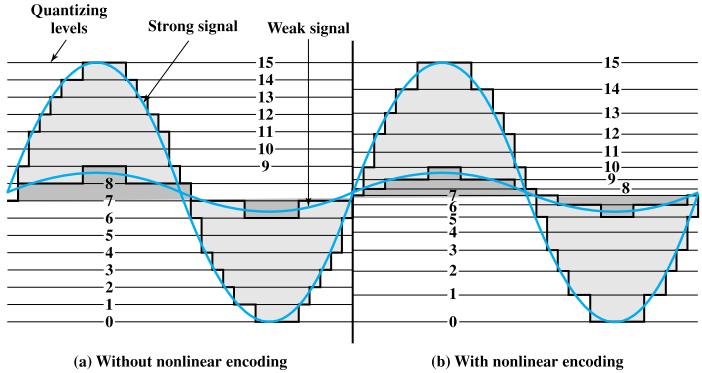
57 Uniform/Non-uniform Quantization

58 Non-uniform quantization Problems with uniform quantization Only optimal for uniformly distributed signal Real audio signals (speech and music) are more concentrated near zeros Human ear is more sensitive to quantization errors at small values Solution Using non-uniform quantization quantization interval is smaller near zero

59 Non-uniform quantizers Quantizing intervals are not uniform In general, Δ i Δ j for i j Suitable when the input signal is not uniformly distributed E.g., Gaussian distribution,...

60 Non-uniform quantizers A non-uniform quantizer can be designed as: A pre-defined function Q(x) written to map input and output using different quantization intervals, or: A Companding quantizer

61 Companding Quantization A compander consists of three stages: Compression Uniform quantization Expansion

62 Companding quantization Compression The input signal is compressed with a nonlinear characteristic C (e.g., C(x)=log(x)) Uniform Quantization The compressed signal is quantized with the uniform characteristc Q Expansion The uniformly quantized signal is expanded inversely with the expansion characteristic E=C 1

63 Companding quantization Compression Uniform quantization Expansion Resulting quantizer

64 Companding quantization The result of this process is a non-uniform quantizer: x Q n (x) = E(Q(C(x)))

65 Companding vs non-linear Q(x) Non-linear Q(x): Faster then companding: the function Q(x) is immediately applicable to the input x Design is not straightforward we need algorithms for adaptive quantization Companding quantizer: Not faster than non-linear Q(x) logarithmic functions must be applied to transform x But look-up tables can be built to speed-up calculations Design and implementation are simpler modular architecture, we just need to configure the function C(x), the rest is a classic uniform quantizer

66 Companding quantizer: the µ-law µ-law is a configurable compression function used in North America and Japan for telecommunications It generates different uniform quantizations by changing the value of µ (N.A. and Japan use µ= 255)

67 µ-law quantizer Compression: compress the sample value x with the formula: x Xmax log 1 + μ log 1 + μ y = C(x) = sgn(x) Uniform Quantization: quantize y with a uniform R-bits quantizer: y = Q(y) Expansion: transform back the value of y using the inverse formula: x = C 1 (y ) = sgn(y ) Xmax μ log 1+μ 10 Xmax y 1

68 Exercise For the following sequence {1.2,-0.2,-0.5,0.4,0.89,1.3 }, Quantize it using a µ -law quantizer (with µ = 9), in the range of [-1.5,1.5] with 4 levels and, and write: the quantized sequence the sequence of binary codes the quantization error for each sample Solution (indirect method): apply the inverse formula to the partition and reconstruction levels found for the uniform quantizer at 4 levels. Because the mu-law mapping is symmetric, we only need to find the inverse values for y = 0.375, 0.75, μ=9, Xmax=1.5, >0.1297, 0.75->0.3604, > Then quantize each sample using the above partition and reconstruction levels.

69 Exercise x = C 1 y = sgn(y ) Xmax 10 μ log 1+μ Xmax y For example: C -1 (-1.125)= sgn log = = = = 0.767

70 µ-law quantizer Uniform, M = 6 µ-law, M = 6; µ= 16

71 A-Law Companding quantizer A-Law is the compression function used in Europe for telecommunications When connecting international systems, A- Law becomes the standard over the µ-law It generates different uniform quantizations by changing the value of compression parameter A (in Europe, A= 87.7, or A= 87.6) Same principles as µ-law, using the following compression and decompression functions:

72 Exercise (for home!) For the following sequence {1.2,-0.2,-0.5,0.4,0.89,1.3 }, Quantize it using a A -law quantizer (with A = 87.7), in the range of [-1.5,1.5] with 4 levels and, and write: the quantized sequence the sequence of binary codes the quantization error for each sample Solution (indirect method): apply the inverse formula to the partition and reconstruction levels found for the uniform quantizer at 4 levels. Because the A-law mapping is symmetric, we only need to find the inverse values for y = 0.375, 0.75, Then quantize each sample using the above partition and reconstruction levels. A=87.7, Xmax= 1.5, >?, >?, >?

73 Adaptive Quantization

74 Adaptive quantization Adaptive quantization allows non-uniform quantizers to decrease the average distortion by assigning more levels to more probable regions. For given M and input pdf, we need to choose {x i } and {y i } to minimize the distortion

75 Lloyd-Max Scalar Quantizer Also known as pdfoptimized quantizer For given M, to reduce MSE (σ q 2 ), we want narrow regions when f(x) is high and wider regions when f(x) is low x 0 x 1 x 2 x 3 x 4 x 5 pdf Given M, the optimal bi and yi that minimize MSE satisfy the Lagrangian condition: σ q 2 regions σ q 2

76 Lloyd-Max Scalar Quantizer Solving the differential equations, we obtain the Lloyd-Max conditions: y i = x i x i 1 x i x i 1 xf x dx f x dx x i = y i + y i+1 2 x i-1 x i X i+1 Given {x i }, it is easy to calculate {y i } Given {y i }, it is easy to calculate {x i } Problem: How can we calculate {x i } and {y i } simultaneously? {x i } depends on {y i }; at the same time {y i } depends on {x i } Solution: iterative method

77 An iterative algorithm known as the Lloyd algorithm solves the problem by iteratively optimizing the encoder and decoder until both conditions are met with sufficient accuracy. The Lloyd Algorithm

78 Lloyd-Max Scalar Quantizer Input: threshold ε Output: values of {y i } and {x i } 1. Initialize all y i ; let j = 1; d 0 = + (distortion). 2. Update all decision levels: 3. Update all y i : y i = 4. Compute MSE (d j ): x i x i 1 x i x i 1 x i = y i + y i+1 2 xf x dx f x dx 5. If d j 1 d j < ε, stop. d j 1 otherwise, set j = j + 1; go to step 2

79 Adaptive quantization Adaptive quantization can be used to reduce the number of colors of an image to a finite number (e.g. 256 for GIF). 7 colors

80 Vector quantization

81 Vector quantization Quantization can be extended to more than one dimension: Scalar quantizer quantizes one sample at a time Vector quantizer quantizes a vector of N samples into a vector of N quantized values Useful when: Input signals show a strong correlation to the patterns stored into the quantizer vectors The sampled signal has codomain with cardinality > 1, e.g. R 3 Mostly used for: Color quantization: Quantize all colors appearing in an image to L (few) colors Image quantization: Quantize every NxN block into one of the L typical patterns (obtained through training).

82 Vector quantization The encoder is loaded with a Codebook: list of predetermined quantizer vectors, each one with an associated index The same Codebook is loaded in the decoder

83 Vector quantization Encoding: given an input vector of N consecutive signal samples, the encoder searches for the most similar vector in the codebook The corresponding index is stored as the output

84 Vector quantization Decoding: the decoder receives the encoded index, and retrieves the corresponding vector in the codebook as reconstruction levels

85 Vector quantization Performance of VQ is asymmetric: Encoding is a heavy process: not straightforward to find the closest vector in the codebook Decoding is very easy: just the retrieval of an indexed vector

86 Encoding performance Encoding: comparing an input vector I v, to all the vectors in the Codebook (V 1, M ), to find the closest one (1-NN) We must calculate the distance between I v and all the M Codebook vectors Distance measure: usually euclidean distance Given two vectors: N V1= <x 1, x 2,, x n > 2 V2= <y 1, y 2,, y n > d V 1, V 2 = x i y i i=1 This is also the Quantization Error!

87 Encoding performance Complexity - if the vectors contain N elements each, and the Codebook contains M vectors: The complexity of calculating the Euclidean Distance on 2 vectors is linear in N Θ(N) Calculating Euclidean Distance between Iv and all the M Codebook vectors is Θ(N*M)

88 Encoding performance But: Quantizing at R bits, means that we have M = 2 R Therefore, the encoder must perform the search of the most closest vector with time: Θ(N* 2 R ) The encoder performance is esponential in the number of bits R!

89 Decoder performance Decoder complexity: the decoder receives the Codebook index, therefore it can immediately retrieve the quantized vector: Θ(1) Many encoders/decoders for video, images and audio have asymmetric performance!!!

90 Quantization Codebook The simplest Codebook can be generated dividing the N-space in M equally shaped regions

91 Quantization Codebook Adaptive techniques can be applied to find the best subdivision of the N-dimensional space, to minimize the quantization error: Adaptive clustering of image samples/colors Generalized Lloyd algorithm

92 Exercise Given the following Codebook, with M = 4 (2 bits): INDEX X1 X2 X And given the following input vectors: <1, 4, 3> <2, 2, 2> <1, 2, 3> <5, 4, 2> Write: The sequence of quantization indexes The quantization error for each vector

93 Reconstruction: main techniques

94 Reconstruction Signal Decoder: Sometimes, it is necessary to convert a digital signal into an analog one: A PC sound card must do it in order to let sounds to be heard through speakers Signal decoders apply different techniques to reconstruct the original signal, using only the sampled and quantized data. The main techniques include: Zero-order hold Linear interpolation Ideal interpolation

95 Zero-order hold the value of the each sample y(n) is held constant for duration T: x(t) = y(n) for the time interval [nt, (n+1)t]

96 Linear interpolation Intuitively, this converter connects the samples with straight lines in the time interval [nt, (n+1)t] x(t)= segment connecting y(n) to y(n+1),

97 Ideal interpolation This converter calculates a smooth curve that passes through the samples The curve can be calculated with methods from numerical analysis. For example, Fourier polynomials or piecewise polynomials (spline)