Dimensionality Reduction and Manifold Learning. Tu Bao Ho Japan Advance Institute of Science and Technology John von Neumann Institute, VNU-HCM

Transcription

1 Dimensionality Reduction and Manifold Learning Tu Bao Ho Japan Advance Institute of Science and Technology John von Neumann Institute, VNU-HCM 1

2 Introduction The background The data is high-dimensional The desire of projecting those data onto a lower-dimensional subspace without losing importance information regarding some characteristic of the original variables The methods Accomplishing the reduction of dimensionality through variable selection, referred to as feature selection. Accomplishing the reduction of dimensionality by creating a reduced set of linear or nonlinear transformations of the input variables, referred to as feature extraction. 2

3 Linear techniques Transformations R p R k, x 1,, x p s 1,, s k, k p, and result in each of the k p components of the new variable being a linear combination of the original variables: s i = w i1 x w ip x p for i = 1,, k or s = Wx where W k p is the linear transformation weight matrix. Expressing the same relationship as x = As with A p k, new variables s are also the hidden or the latent variables. In terms of an n p observation matrix X, we have S ij = w i1 X 1j + + w ip X pj for i = 1,, k; j = 1,, n where j indicates the jth realization, or, equivalently, S k n = W k p X p n, X p n = A p k S k n 3

4 Content A. Linear dimensionality reduction 1. Principal component analysis (PCA) 2. Independent component analysis (ICA) 3. Factor analysis 4. Canonical variate analysis 5. Projection pursuit B. Nonlinear dimensionality reduction 6. Polynomial PCA 7. Principal curves and surfaces 8. Kernel PCA 9. Multidimensional scaling 10. Nonlinear manifold learning 4

5 Principal component analysis (PCA) PC is also known as the singular value decomposition (SVD), the Karhunen-Loève transform, the Hotelling transform (1933), and the empirical orthogonal function (EOF) method. PCA reduces the dimension by finding a few orthogonal linear combinations (the PCs) of the original variables with the largest variance (PCA giảm số chiều bằng cách tìm ra một số nhỏ các tổ hợp tuyến tính trực giao (PC) của các biến gốc với phương sai lớn nhất) The first PC, s 1, is the linear combination with the largest variance s 1 = x τ w 1, where coefficient vector w 1 = w 11,, w 1p τ solves w 1 = arg max w=1 Var x τ w The second PC, s 2, is the linear combination with the second largest variance and orthogonal to the first PC, and so on. There are as many PCs as the number of the original variables. 5

6 Principal component analysis The first several PCs may explain most of the variance, so that the rest can be disregarded with minimal loss of information. As variance depends on the variable scale, first standardize each variable to have mean zero and standard deviation one. Assuming a standardized data with the empirical covariance matrix Σ p p = 1 n XXτ We can use the spectral decomposition theorem to write Σ as Σ = UΛU τ where Λ = diag(λ 1,, λ p ) is the diagonal matrix of the ordered eigenvalues λ 1 λ p, and U is a p p orthogonal matrix containing the eigenvectors. 6

7 Principal component analysis Property 1. The subspace spanned by the first k eigenvectors has the smallest mean square deviation (độ lệch trung bình bình phương nhỏ nhẩt) from X among all subspaces of dimension k (Mardia et al., 1995). Property 2. The total variation in the eigenvalue decomposition is equal to the sum of the eigenvalues of the covariance matrix, (sai khác toàn bộ trong phân tích gía trị riêng bằng tổng các vector riêng của ma trận phương sai) and the fraction p i=1 p Var PC i = λ i = trace(σ) k i=1 λ i i=1 trace(σ) gives the cumulative proportion of the variance explained by the first k PCs (tỷ lệ tích lũy của biến đổi tính theo k PC đầu tiên). 7 p i=1

8 Principal component analysis By plotting the cumulative proportions in as a function of k, one can select the appropriate number of PCs to keep in order to explain a given percentage of the overall variation. An alternative way to reduce the dimension of a dataset using PCA: Instead of using the PCs as the new variables, this method uses the information in the PCs to find important variables in the original dataset. Another way: The number of PCs to keep is determined by first fixing a threshold λ 0, then only keeping the eigenvectors (at least four) such that their corresponding eigenvalues are greater than λ 0 (Jolliffe, 1972, 1973). 8

9 Principal component analysis Example Nutritional data from 961 food items. The nutritional components of each food item are given by seven variables: fat (grams), food energy (calories), carbohydrates (grams), protein (grams), cholesterol (milligrams), weight (grams), and saturated fat (grams). PCA of the transformed data yields six principal components ordered by decreasing variances. The first three principal components, PC1, PC2, and PC3, which account for more than 83% of the total variance 9

10 Principal component analysis Example 10

11 Independent component analysis (ICA) A method that seeks linear projections, not necessarily orthogonal to each other, but nearly statistically independent as possible. The random variables x = x 1,, x p are uncorrelated, if for i j, 1 i, j p, we have Cov x i, x j = 0. Independence requires that the multivariate probability density function factorizes, f x 1,, x p = f 1 x 1 f p (x p ). independence uncorrelated, but uncorrelated independence. The noise-free ICA model for the p-dimensional random vector x seeks to estimate the components of the k-dimensional vector s and the p k full column rank mixing matrix A τ x 1,, x p = Ap k s 1,, s τ k such that the components of s are as independent as possible, according to some definition of independence. 11

12 Independent component analysis (ICA) The noisy ICA contains an additive random noise component, x 1,, x p τ = Ap k s 1,, s k τ + u 1,, u p τ Estimation of such models is still an open research issue. In contrast with PCA, the goal of ICA is not necessarily dimension reduction. To find k < p independent components, one needs to first reduce the dimension of the original data p to k, by a method such as PCA. No order among the PCs of ICA. ICA can be considered a generalization of the PCA and the PP (project pursuit) concepts. ICA is applied to many different problems, including exploratory data analysis, blind source separation, blind deconvolution, and feature extraction. 12

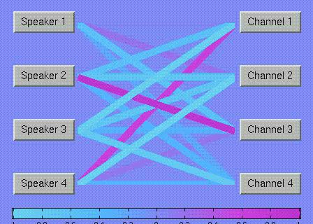
13 Independent component analysis (ICA) Perform ICA Mic 1 Mic 2 Mic 3 Mic 4 Terry Te-Won Scott Tzyy-Ping Play Mixtures Play Components 13

14 Factor analysis (FA) A linear method, based on the second-order data summaries. Factor analysis assumes that the measured variables depend on some unknown, and often unmeasurable, common factors. Typical examples include variables defined as various test scores of individuals, as such scores are thought to be related to a common intelligence" factor. The goal of FA is to uncover such relations, and thus can be used to reduce the dimension of datasets following the factor model. The zero-mean p-dimensional random vector x p 1 with covariance matrix Σ satisfies the k-factor model x = Λf + u where Λ p k is a matrix of constants, and f k 1 and Λ p k and u p 1 are the random common factors and specific factors, respectively. 14

15 Canonical variate analysis (CVA, Hotelling, 1936) A method for studying linear relationships between two vector variates, X = X 1,, X r τ and Y = Y 1,, Y s τ which have different dimensions. CVA seeks to replace the two sets of correlated variables, X and Y, by t pairs of new variables, ξ i, ω i, i = 1,, t; t min r, s where ξ i = g j τ X = r k=1 g kj X k, ω i = h j τ Y = kj Y k s k=1 15

16 Canonical variate and correlation analysis Least-squares optimality of CVA The task X 1,, X r, Y 1,, Y s τ ξ 1, ω 1,, ξ t, ω t τ Linear projections by t r -matrix G and t s -matrix H with 1 t min r, s : ξ = GX, ω = HY, Least-square error criterion, to find ν, G, and H so that to minimize HY ν + GX E HY ν + GX HY ν + GX τ which measure how well we can reconstruct X and Y from pairs of ξ i, ω i The goal is To choose the best ν, G, and H in the least-square sense. 16

17 Projection Pursuit Phép chiếu đuổi The motivation The desire to discover interesting low-dimensional (typically, one- or two-dimensional) linear projections of high-dimensional data The origin The desire to expose specific non-gaussian features (variously referred to as local concentration, clusters of distinct groups, clumpiness, or clottedness ) of the data. The strategy 1. Set up a projection index I to judge the merit of a particular one or two-dimensional (or sometimes three-dimensional) projection of a given set of multivariate data. 2. Use an optimization algorithm to find the global and local extrema of that projection index over all m-dimensional projections of the data. 17

18 Projection Pursuit Projection Indexes Projection indexes should be chosen to possess certain computational and analytical properties, especially that of affine invariance (location and scale invariance). A special case of PP occurs when the projection index is the variance. Maximizing the variance reduces PP to PCA, and the resulting projections are the leading principal components of X. Maximizing the variance is equivalent to minimizing the corresponding Gaussian log-likelihood; in other words, the projection is most interesting (in a variance sense) when X is least likely to be Gaussian. Typical PP: Cumulant-based index Polynomial-based indexes Shannon negentropy Optimizing the projection index 18

19 Introduction The linear projection methods can be extremely useful in discovering low-dimensional structure when the data actually lie in a linear (or approximately linear) lower-dimensional subspace M (called a manifold) of input space R r. What can we do if we know or suspect that the data actually lie on a low dimensional nonlinear manifold, whose structure and dimensionality are both assumed unknown? Dimensionality reduction Problem of nonlinear manifold learning. When a linear representation of the data is unsatisfactory, we turn to specialized methods designed to recover nonlinear structure. Even so, we may not always be successful. Key ideas: Generalizing linear multivariate methods. Note that, these equivalences in the linear case do not always transfer to the nonlinear case. (tổng quát hóa các pp tuyến tính đa biến dù không luôn thành công). 19

20 Polynomial PCA How should we generalize PCA to the nonlinear case? One possibility is to transform the set of input variables using a quadratic, cubic, or higher degree polynomial, and then apply linear PCA. Focused on the smallest few eigenvalues for nonlinear dimensionality reduction. Quadratic PCA: the r-vector X is transformed into an extended r-vector X, where r = 2r + r(r 1)/2, X = (X 1, X 2 ) X = (X 1, X 2, X 1 2, X 2 2, X 1 X 2 ) Some problems inevitably arise when using quadratic PCA. First, the variables in X will not be uniformly scaled, especially for large r, and so a standardization of all r variables may be desirable. Second, the size of the extended vector X for quadratic PCA increases quickly with increasing r: when r = 10, r = 65, and when r = 20, r =

21 Principal curves and surfaces Suppose X is a continuous random r-vector having density p X, zero mean, and finite second moments. Suppose further that the data observed on X lie close to a smooth nonlinear manifold of low dimension. A principal curve (Hastie, 1984; Hastie and Stuetzle, 1989) is a smooth one-dimensional parameterized curve f that passes through the middle of the data, regardless of whether the middle is a straight line or a nonlinear curve. A principal surface is a generalization of principal curve to a smooth two-(or higher-) dimensional curve. We use an analogue of least-squares optimality as the defining characteristic: we determine the principal curve or surface by minimizing the average of the squared distances between the data points and their projections onto that curve. 21

22 Content A. Linear dimensionality reduction 1. Principal component analysis (PCA) 2. Independent component analysis (ICA) 3. Factor analysis 4. Canonical variate analysis 5. Projection pursuit B. Nonlinear dimensionality reduction 6. Polynomial PCA 7. Principal curves and surfaces 8. Kernel PCA 9. Multidimensional scaling 10. Nonlinear manifold learning 22

23 Introduction A map including cities and towns table where each cell shows the degree of closeness (or proximity, sự gần gũi) of a row city to a column city. Proximity could have different meanings: straight-line distance or as shortest traveling distance. Consider entities as objects, products, a nations, a stimulus, etc. and we can talk about proximity of any two entities as measures of association (e.g., absolute value of a correlation coefficient), confusion frequency (i.e., to what extend one entity is confused with another in an identification exercise), or measure of how alike (or how different), etc. Multidimensional scaling (MDS): [tái dựng bản đồ gốc nhiều chiều] given a table of proximities of entities, reconstruct the original map of entities as closely as possible. MDS is a family of different algorithms, each designed to arrive at an optimal low-dimensional configuration for a particular type of proximity data. 23

24 Introduction Problem: Re-create the map that yielded the table of airline distances. Airline distances (km) between 18 cities. Source: Atlas of the World, Revised 6th Edition, National Geographic Society, 1995, p. 131 Two and three dimensional map of 18 world cities using the classical scaling algorithm on airline distances between those cities. The colors reflect the different continents: Asia (purple), North America (red), South America (orange), Europe (blue), Africa (brown), and Australasia (green). 24

25 Examples of MDS applications Marketing: Derive product maps of consumer choice and product preference (e.g., automobiles, beer) so that relationships between products can be discerned Ecology: Provide environmental impact maps of pollution (e.g., oil spills, sewage pollution, drilling-mud dispersal) on local communities of animals, marine species, and insects. Molecular Biology: Reconstruct the spatial structures of molecules (e.g., amino acids) using biomolecular conformation (3D structure). Interpret their interrelations, similarities, and differences. Construct a 3D protein map as a global view of the protein structure universe. Social Networks: Develop telephone-call graphs, where the vertices are telephone numbers and the edges correspond to calls between them. Recognize instances of credit card fraud and network intrusion detection. 25

26 Proximity matrices The focus on pairwise comparisons of entities is fundamental to MDS. The closeness of two entities is measured by a proximity measure, defined in a number of different ways. A continuous measure of how physically close one entity is to another or a subjective judgment recorded on an ordinal scale, but where the scale is well-calibrated as to be considered continuous. In perception study, proximity is not quantitative but a subjective rating of similarity (or dissimilarity) recorded on a pair of entities. Closeness of one entity to another could be measured by a small or large value. Importance is a monotonic relationship between the closeness of two entities. 26

27 Proximity matrices Collection of n entities. Let δ ij represent the dissimilarity of the ith entity to the jth entity. Consider m dissimilarities, m = n 2 = 1 n n 1, and 2 (m m) proximity matrix Δ = (δ ij ) (1) The proximity matrix is usually displayed as a lower-triangular array of nonnegative entries, with the understanding that the diagonal entries are all zeroes and the matrix is symmetric: for all i, j = 1,..., n, δ ij 0, δ ii = 0, δ ji = δ ij In order for a dissimilarity measure to be regarded as a metric distance, we require that δ ij satisfy the triangle inequality, δ ij δ ik + δ kj for all k 27

28 Comparing protein sequences Optimal sequence alignment About 100,000 different proteins in the human body. Proteins carry out important bodily functions: supporting cell structure, protecting against infection from bacteria and viruses, aiding movement, transporting materials (hemoglobin for oxygen), regulating control (enzymes, hormones, metabolism, insulin) of the body. protein map : how existing protein families relate to one another, structurally and functionally. Might be able to predict the functions of newly discovered proteins from their spatial locations and proximities to other proteins, where we would expect neighboring proteins to have very similar biochemical properties. 28

29 Comparing protein sequences Optimal sequence alignment Key idea in computing the proximity of two proteins is amino acids can be altered by random mutations (đột biến) over a long period of evolution. Mutations can take various forms: deletion or insertion of amino acids, For an evolving organism to survive, structure/functionality of the most important segments of its protein would have to be preserved. Compute a similarity value between two sequences that have different lengths and different amino acid distributions. Trick: Align the two sequences so that as many letters in one sequence can be matched with the corresponding letters in the other sequence. Several methods for sequence alignment: Global alignment aligns all the letters in entire sequences assuming that the two sequences are very similar from beginning to end; Local alignment assumes that the two sequences are highly similar only over short segments of letters. 29

30 Comparing protein sequences Optimal sequence alignment Alignment methods use dynamic programming algorithms as the primary tool. BLAST and FASTA are popular tools for huge databases. An optimal alignment if maximizing an alignment score. For example, an alignment score is the sum of a number of terms, such as identity (high positive), substitution (positive, negative or 0). Substitution score: cost of replacing one amino acid (aa). Scores for all 210 possible aa pairs are collected to form a (20 20) substitution matrix. One popular is BLOSUM62 (BLOcks Substitution Matrix), assuming no more than 62% of letters in sequences are identical (Henikoff, 1996). A gap (indel), an empty space ( - ), penalizes an insertion or a deletion of an aa. Two types of gap penalties, starting a gap and extending the gap. The alignment score s is the sum of the identity and substitution scores, minus the gap score. 30

31 Comparing protein sequences Example: Two hemoglobin chains Given n proteins, let s ij be the alignment score between the ith and jth protein. We have δ ij = s max s ij, where s max is the largest alignment score among all pairs. The proximity matrix is then given by Δ = (δ ij ). Compare the hemoglobin alpha chain protein HBA HUMAN having length 141 with the related hemoglobin beta chain protein HBB HUMAN having length 146. We would obtain different optimal alignments and alignment scores. 86 positive substitution scores (the 25 + s and the 61 identities). The alignment score is s =

32 String matching Edit distance In pattern matching, we study the problem of finding a given pattern within a body of text. If a pattern is a single string, the problem is called string matching, used extensively in text-processing applications. A popular numerical measure of the similarity between two strings is edit distance (also called Levenshtein distance). The usual definition of edit distance is the fewest number of editing operations (insertions, deletions, substitutions) which would be needed to transform one string into the other. An insertion inserts a letter into the sequence, a deletion deletes a letter from the sequence, and a substitution replaces one letter in the sequence by another letter. Identities (or matches) are not counted in the distance measure. Each editing operation can be assigned a cost. Used to construct a phylogenetic tree a diagram laying out a possible evolutionary history of a single protein. 32

33 Classical scaling and distance geometry Suppose we are given n points X 1,...,X n R r. From these points, we compute an (n n) proximity matrix Δ = (δ ij ) of dissimilarities, where r δ ij = X i X j = k=1(x ik X jk ) 2 1/2 (2) Many kinds of distance can be considered: the Minkowski or L p distance is given by r δ ij = X ik X p k=1 jk p = 1: city-block or Manhattan distance, 1/p p = 2: Euclidean distance. 33

34 Classical scaling and distance geometry From dissimilarities to principal coordinates From (2), σ ij 2 = X i 2 + X j 2 2Xi τ X j. Let b ij = X i τ X j = 1 2 (δ ij 2 δ i0 2 δ j0 2 ) where δ i0 2 = X i 2. We get b ij = a ij a i. a.j + a ii where a ij = 1 2 δ ij 2, a i. = n 1 2 a ij 2 2 i. j, a.j = n 1 i a ij, a.. = n 2 j a ij If setting A = a ij the matrix of squared dissimilarities and B = b ij, we have B = HAH where H = I n n 1 J n, J n is square matrix of ones. Wish to find a t dimensional representation, Y 1,...,Y n ϵ R t (referred to as principal coordinates), of those r-dimensional points (with t < r), such that the interpoint distances in t-space match those in r-space. When dissimilarities are defined as Euclidean interpoint distances, this type of classical MDS is equivalent to PCA in that the principal coordinates are identical to the scores of the first t principal components of the {X i }. 34

35 Classical scaling and distance geometry From dissimilarities to principal coordinates Typically, in classical scaling (Torgerson, 1952, 1958) we are not given *X i + ϵ R t ; instead, we are given only the dissimilarities *δ ij + through the (n n) proximity matrix Δ. Using Δ, we form A, and then B. Motivation for classical scaling comes from a least-squares argument similar to the one employed for PCA. The classical scaling algorithm is based upon an eigendecomposition of the matrix B. This eigendecomposition produces Y 1,...,Y n ϵ R t, t < r, a configuration whose Euclidean interpoint distances, d 2 2 τ ij = Y i Y j = Yi Y j (Yi Y j ) The solution of the classical scaling problem is not unique. A common orthogonal transformation of the points in the configuration found by classical scaling yields a different solution of the classical scaling problem. 35

36 Classical scaling The classical scaling algorithm 36

37 Classical scaling and distance geometry Airlines distances Eigenvalues of B and the eigenvectors corresponding to the first three largest eigenvalues (in red) for the airline distances example. First three principal coordinates of the 18 cities in the airline distances example. Estimated and observed airline distances. The lefnels show the 2D solution and the right panels show the 3D solution. The top panels show the estimated distances plotted against the observed distances, and the bottom panels show the residuals from the the fit (residual = estimated distance observed distance) plotted against sequence number. 37

38 Classical scaling and distance geometry Mapping the protein universe 92 b-sheet proteins 94 a/b-sheet proteins The first 25 ordered eigenvalues of B obtained from the classical scaling algorithm on 498 proteins. 498 proteins classical scaling algorithm largest 25 eigenvalues of B first three eigenvalues are dominant 3D configuration is probably most appropriate. 2D map and 3D map 136 a-helix proteins 92 a+b-sheet proteins Two-dimensional map of four protein classes using the classical scaling algorithm on 498 proteins. A three-dimensional map of four protein classes using the classical scaling algorithm on 498 proteins. 38

39 Distance scaling Given n items (or entities) and their dissimilarity matrix s, Δ = (δ ij ) Classical scaling problem is to find a configuration of points in a lowerdimensional space such that the interpoint distances {d ij } satisfy d ij δ ij. In distance scaling, this relationship is relaxed; we wish to find a suitable configuration for which d ij f(δ ij ) where f is some monotonic function. The function f transforms the dissimilarities into distances. The use of metric or nonmetric distance scaling depends upon the nature of the dissimilarities. If the dissimilarities are quantitative we use metric distance scaling, whereas if the dissimilarities are qualitative we use nonmetric distance scaling. In the MDS literature, metric distance scaling is traditionally called metric MDS, nonmetric distance scaling is called nonmetric MDS. 39

40 Summary Introduction: Given a table of proximities, reconstruct the original map as closely as possible and the space dimension. Proximity Matrices: Δ = (δ ij ) measures closeness of pairwise objects, metric (triangle inequality) Comparing Protein Sequences String Matching: Edit distance Classical Scaling: require d ij δ ij Distance Scaling: d ij f(δ ij ) where f is monotonic Metric Distance Scaling: metric distance scaling Nonmetric Distance Scaling: nonmetric distance scaling 40

41 Nonlinear manifold learning Manifold? An ant at a picnic: The ant crawls all over the picnic items, as diminutive size, the ant sees everything on a very small scale as flat and featureless. A manifold can be thought of in similar terms, as a topological space that locally looks flat and featureless and behaves like Euclidean space. A manifold also satisfies certain topological conditions. A submanifold is just a manifold lying inside another manifold of higher dimension. 41

42 Nonlinear manifold learning Many exciting new algorithmic techniques: Isomap, Local Linear Embedding, Laplacian Eigenmap, and Hessian Eigenmap. They aim to recover the full low-dimensional representation of an unknown nonlinear manifold M. Having different philosophies for recovering nonlinear manifolds, each methods consists of a three-step approach. 1) Incorporating neighborhood information from each data point to construct a weighted graph having the data points as vertices. 2) Taking the weighted neighborhood graph and transforming it into suitable input for the embedding step. 3) Computing an (n n)-eigenequation (embedding step). Manifold learning involves concepts from differential geometry: What means a manifold and what means to be embedded in a higherdimensional space? 42

43 Nonlinear manifold learning If a topological manifold M is continuously differentiable to any order (i.e., M C ), we call it a smooth (or differentiable) manifold. Riemannian manifold (M, d M ) is smooth manifold M with a metric d M. We take d M to be a manifold metric defined by d M y, y = inf* L(c) c is a curve in M which joins y and y +, c where y, y M and L(c) is the arc-length of the curve c. Thus, d M finds the shortest curve (or geodesic, đo đạc) between any two points on M, and the arc-length of that curve is the geodesic distance between the points. Data assumption: Finitely many data points, *y i +, are randomly sampled from a smooth t-dimensional manifold M with metric given by geodesic distance. 43

44 Nonlinear manifold learning ISOMAP The isometric feature mapping (or ISOMAP) algorithm (Tenenbaum et al., 2000) assumes that the smooth manifold M is a convex region of R t (t r) and that the embedding ψ : M X is an isometry. This assumption has two key ingredients: Isometry: The geodesic distance is invariant under the map ψ. For any pair of points on the manifold, y, y M, the geodesic distance between those points equals the Euclidean distance between their corresponding coordinates, x, x X; i.e., where y = φ(x) and y = φ(x ). d M (y, y ) = x x X Convexity: The manifold M is a convex subset of R t. ISOMAP regards M as a convex region that may have been distorted in any of a number of ways (e.g., by folding or twisting), e.g., Swiss roll. isometry is a distance-preserving map between metric spaces. 44

45 Nonlinear manifold learning Three steps of ISOMAP 1. Neighborhood graph. Fix either an integer K or an ε > 0. Calculate the distances, d ij M = d X x i, x j = x i x j X between all pairs of data points x i, x j X, i, j = 1, 2,..., n. Determine which data points are neighbors on the manifold M by connecting each point either to its K nearest neighbors or to all points lying within a ball of radius ε of that point. Choice of K or ε controls neighborhood size and also the success of ISOMAP. We obtain weighted neighborhood graph G = G(V, E), where the set of vertices V = x 1,, x n are the input data points, and the set of edges E = *e ij + indicate neighborhood relationships between the points. 45

46 Nonlinear manifold learning Three steps of ISOMAP 2. Compute graph distances Estimate the unknown true geodesic distances, d ij M, between pairs of points in M by graph distances, d ij G, with respect to the graph G. The graph distances are the shortest path distances between all pairs of points in the graph G. Points that are not neighbors of each other are connected by a sequence of neighbor-to-neighbor links. An efficient algorithm for computing the shortest path between every pair of vertices in a graph is Floyd s algorithm (Floyd, 1962), which works best with dense graphs (graphs with many edges). 46

47 Nonlinear manifold learning Three steps of ISOMAP 3. Embedding via multidimensional scaling Let D G = d ij G be the symmetric n n -matrix of graph distances. Apply classical MDS to D G to give the reconstructed data points in a t-dimensional feature space Y, so that the geodesic distances on M between data points is preserved as much as possible: Form the doubly centered, symmetric, (n n)-matrix of squared graph distances. The embedding vectors *y i } are chosen to minimize A n G An Y G 1 where A n = 2 HSG Y 1 H and A n = H d Y 2 Y 2 ij H and d ij = y i y j. The graph G is embedded into Y by the (t n)-matrix Y = y 1,, y n = ( λ 1 v 1,, λ t v t ) τ 47

48 Nonlinear manifold learning Examples Two-dimensional LANDMARK ISOMAP embedding, with neighborhood graph, of the complete set of n = 20,000 Swiss-Roll data points. The number of neighborhood points is K = 7, and the number of landmark points is m = 50. Two-dimensional ISOMAP embedding, with neighborhood graph, of the n = 1,000 Swiss roll data points. The number of neighborhood points is K = 7. Two-dimensional LANDMARK ISOMAP embedding, with neighborhood graph, of the n = 1,000 Swiss roll data points. The number of neighborhood points is K = 7 and the number of landmark points is m =