Electromechanical Characterization of the Static and Dynamic Response of Dielectric Elastomer Membranes

Transcription

1 Electromechanical Characterization of the Static and Dynamic Response of Dielectric Elastomer Membranes by Jason William Fox Thesis submitted to the faculty of the Virginia Polytechnic Institute and State University in partial fulfillment of the requirements for the degree of Master of Science in Mechanical Engineering Nakhiah Goulbourne, Chair Daniel Inman Mary Kasarda August 31 st, 7 Blacksburg, Virginia Keywords: Dynamic Membrane, Static Membrane, Dielectric Elastomer, Diaphragm Inflation, Large Deformations, Capacitance Sensing

2 Electromechanical Characterization of the Static and Dynamic Response of Dielectric Elastomer Membranes Jason William Fox Abstract Dielectric elastomers (DEs) are a relatively new electroactive polymer (EAP) transducer technology. They are capable of over 1% strain when actuated, and can be used as sensors to measure large strains. In actuation mode, the DE is subject to an electric field; in sensing mode, the capacitance of the dielectric elastomer is measured. In this work, a dielectric elastomer configured as a circular membrane clamped around its outer edge over a sealed chamber and inflated by a bias pressure is studied in order to characterize its static and dynamic electromechanical behavior. In both cases, the experiments were conducted with prestretched dielectric elastomer actuators fabricated from.5 mm or 1 mm thick polyacrylate films and unless stated otherwise carbon grease electrodes were used. The static tests investigate the effect of flexible electrodes and passive layers on the electromechanical response of dielectric elastomer membrane actuators and sensors. To study the effect of the flexible electrodes, four compliant electrodes were tested: carbon grease, silver grease, graphite spray, and graphite powder. The electrode experiments show that carbon grease is the most effective electrode of those tested. To protect the flexible electrodes from environmental hazards, the effect of adding passive elastic layers to the transducers was investigated. A series of tests were conducted whereby the position of the added layers relative to the transducer was varied: (i) top passive layer, (ii) bottom passive layer, and (iii) passive layers on both the bottom and top of the transducer. For the passive layer tests, the results show that adding elastic layers made of the same material as the DE

3 dramatically changes both the mechanical and electrical response of the actuator. The ability to use capacitance measurements to determine the membrane s maximum stretch was also investigated. The experiments demonstrate that the capacitance response can be used to sense large mechanical strains in the membrane 5%. In addition, a numerical model was developed which correlates very well with the experimental results especially for strains up to 41%. The dynamic experiments investigate the dynamic response of a dielectric elastomer membrane due to (i) a time-varying pressure input and (ii) a time-varying voltage input. For the time-varying pressure experiments, the prestretched membrane was inflated and deflated mechanically while a constant voltage was applied. The membrane was cycled between various predetermined inflation states, the largest of which was nearly hemispherical, which with an applied constant voltage of 3 kv corresponded to a maximum strain at the pole (center of membrane) of 8%. These experiments show that for higher voltages, the volume displaced by the membrane increases and the pressure inside the chamber decreases. For the time varying voltage experiments, the membrane was passively inflated to various predetermined states, and then actuated. Various experiments were conducted to see how varying certain system parameters changed the membrane s dynamic response. These included changing the chamber volume and voltage signal offset, as well as measuring the displacement of multiple points along the membrane s radius in order to capture its entire motion. The chamber volume experiments reveal that increasing the size of the chamber onto which the membrane is clamped will cause the resonance peaks to shift and change in number. For these experiments, the pole strains incurred during the inflation were as high as 6 %, corresponding to slightly less than a hemispherical state. Upon actuation using a voltage signal with an amplitude of 1.5 kv, the membrane would inflate further, causing a maximum additional strain of 1.1%. The voltage signal offset experiments show that adding offset to the input signal causes the membrane to oscillate at two distinct frequencies rather than one. Lastly, experiments to capture the entire motion of the membrane revealed the different mode shapes the membrane s motion resembles. iii

4 Acknowledgments I would first like to thank my advisor, Dr. Nakhiah Goulbourne, for her support and guidance throughout my time at CIMSS and for always pushing me to do my best. I would also like to thank Dr. Alan Snyder s group in the bioengineering lab at the Hersey Medical Center at Pennsylvania State University for their complimentary research and providing the test chamber initially used for this work. I would like to acknowledge the helpful willingness of Keith Boyd at the Mechanical Utility Facility to supply me in two separate occasions with the 3 section of 1 diameter piping I needed to construct part of my dynamic experimental setup. I would like to thank the people in CIMSS for their advice and help. While everyone has contributed in some way to get me to this point, I would like to extend a particular thanks to both Vishnu Sundaresan, for everything from taking so much of his time to help me work out computer related problems (there were a lot) to letting me stay at his apartment my last month in Blacksburg after my lease expired, and Steve Anton, for showing me all the finer points of Labview. I thank my twin brother, Chris, for always being willing to lend a hand. It is nice to know that I will always have someone that I can trust and confide in. Lastly, I owe much thanks to my mother and father for their encouragement and support throughout the years. They have always been there to guide me and give their advice, and it means a great deal to know that I can count on them for their continued support in years to come. I consider myself extremely fortunate to have such wonderful parents. iv

5 Table of Contents List of Tables... vii List of Figures... viii Nomenclature... xii Chapter 1 Introduction Motivation Dielectric Elastomers DE Membranes Background Scope of Thesis... 7 Chapter Electromechanical Behavior of Dielectric Elastomers Principle of Operation Constitutive Model Dielectric Materials Electrode Materials Constant Load Experiment Model Setup and Procedure Results and Discussion Capacitance-Pole stretch model... Chapter 3 Static Experiments Methods Experimental Setup Specimen Preparation Experimental Procedure Actuation Experiments Electrode Experiments Passive Layer Experiments Sensing Experiments Prestretch Experiments Electrode Experiments Passive Layer Experiments Verification of Sensing Model Chapter 4 Dynamic Experiments Methods Experimental Setups Specimen Preparation v

6 4.1.3 Procedure Dynamic Mechanical Loading Experiments Dynamic Electrical Loading Experiments The Effect of Chamber Volume on DE Membrane Response Offset of the Voltage Signal Overall Motion of the DE Membrane... 9 Chapter 5 Summary and Conclusions Quasi-Static Experiments Dynamic Experiments References Appendix A: Mathematica Codes Appendix B: Labview Codes Appendix C: Matlab Codes Vita vi

7 List of Tables Table 1. Material constants for VHB obtained from uniaxial extenstion test Table. Frequency, volume and voltage values for dynamic mechanical loading experiments Table 3. Chamber volumes tested for membrane stress experiment Table 4. Results from stress state experiment Table 5. In-plane pole stress for the two chamber volumes tested Table 6. Location of resonance peaks for different offsets vii

8 List of Figures Figure 1 Categories and types of electroactive polymers.... Figure. Different DE configurations: Extenders/Bimorphs (a), cylindrical actuators (b), linear actuators (c), inflatable membranes (d), annular membranes (e), and planar configurations (f,g) Figure 3. Actuation of a DE (left) and sensing using a DE (right), where x represents the capacitance of the DE Figure 4. Two-term Ogden model compared against the experimental results generated from a uniaxial stress-strain test Figure 5. Pictures and micrographs of carbon grease (top left), silver grease (top right), graphite spray (lower left) and graphite powder (lower right) Figure 6. Experimental setup for the constant load experiments Figure 7. Photo of experimental setup for the constant load experiments Figure 8. Schematic of a prepared DE actuator for constant load testing Figure 9. Results from constant load experiment.... Figure 1. Experimental results of the electromechanical behavior of the planar DE actuator Figure 11. Model data for constant load experiment Figure 1. Geometry of a spherical cap Figure 13. Experimental setup for static actuation experiments Figure 14. Components of static test fixture... 3 Figure 15. Polymer specimen during prestretch Figure 16. Actuator before and after inflation Figure 17. Cross-sectional view of DE membrane with passive layers added Figure 18. Pressure-volume results for membrane with carbon grease electrodes Figure 19. Pressure-volume results for membrane with silver grease electrodes Figure. Pressure-volume results for membrane with graphite powder electrodes Figure 1. Pressure differences for carbon grease (CG), silver grease (SG), and graphite powder (GP) viii

9 Figure. Comparison of electroded specimens to non-electroded specimens Figure 3. Results of experiments with passive layers compared with the experimental results of a single layer DE Figure 4. Pressure differences for the 4kV case of specimens with passive layers compared with the single layer specimen Figure 5. Pressure Difference for the kv case of specimens with passive layers compared with the single layer specimen Figure 6. Volume differences for the 4kV case of specimens with passive layers compared with the single layer specimen Figure 7. Volume differences for the kv case of specimens with passive layers compared with the single layer specimen Figure 8. Capacitance vs. Time plot for a flat, unstressed DE membrane Figure 9. Experimental results for capacitance and pressure vs. volume for a DE membrane sensor Figure 3. Capacitance-volume results for various prestretches Figure 31. Capacitance-volume results for silver grease and carbon grease Figure 3. Cross-sectional view DE membrane sensor enclosed by passive layers Figure 33. Comparison of Capacitance-volume curves for specimens with and without passive layers Figure 34. Experimental setup for measuring pole stretch Figure 35. Comparison between model and experiment for the sensing of maximum stretch Figure 36. Sections of the piston used in the dynamic mechanical loading tests Figure 37. Test setup for the dynamic mechanical loading experiments Figure 38. Experimental setup used for the dynamic electrical loading tests Figure 39. Circuit used in the dynamic electrical loading experiments Figure 4. Circuit diagram for DE membrane Figure 41. Sample graphs from kv tests... 6 Figure 4. Sample graphs from 1.5 kv tests Figure 43. Sample graphs from 3 kv tests ix

10 Figure 44. Pressure change of the membrane for a 7 ml volume change Figure 45. Displacement of the membrane for a 7ml volume change Figure 46. Static pressure-volume curves for two different chamber volumes Figure 47. Piston positions for chamber volume tests Figure 48. Pole (center of membrane) displacement for a chamber volume of 16ml Figure 49. Frequency response, with labeled resonance peaks, of the DE membrane inflated with an 8 Pa bias pressure at a chamber volume of 47 ml Figure 5. Pole displacement for a chamber volume of 49 ml Figure 51. Pole displacement for a chamber volume of 456 ml Figure 5. Pole displacement for a chamber volume of 178 ml Figure 53. Pole displacement for a chamber volume of 4784 ml Figure 54. Pole displacement for a chamber volume of 185 ml Figure 55. Pole displacement for a chamber volume of 35 ml Figure 56. Magnitude and frequency of resonance frequency A Figure 57. Magnitude and frequency of resonance frequency B Figure 58. Magnitude and frequency of resonance frequency C Figure 59. Magnitude and frequency of resonance frequency D Figure 6. Magnitude and frequency of resonance frequency E Figure 61. Maximum displacement of membrane for each chamber volume tested Figure 6. Maximum pole stretch of membrane for different chamber volumes Figure 63. Pressure change for a chamber volume of 4784 ml Figure 64. Pressure change for a chamber volume of 185 ml Figure 65. Pressure change for a chamber volume of 35 ml Figure 66. Maximum pressure change caused by the membrane as chamber volume is increased Figure 67 Depiction of the path the DE might take during actuation Figure 68. Waveforms produced from the squared voltage signal Figure 69. Frequency response of membrane at a bias pressure of 8 Pa for voltage signals with varying offset x

11 Figure 7. Membrane response at different frequencies for a voltage signal with a kv offset Figure 71. Membrane response at different frequencies for a voltage signal with a.5 kv offset Figure 7. Membrane response at different frequencies for a voltage signal with a 1.5 kv offset Figure 73. Points along the radius of the membrane at which displacement was recorded Figure 74. Frequency response of all nine points for an inflation pressure of 8 Pa Figure 75. Aligned displacement response curves for all nine points Figure 76. Membrane motion at 3 Hz. Displacement has been scaled by Figure 77. Membrane motion at 6.5 Hz. Displacement has been scaled by Figure 78. Membrane motion at 15 Hz. Displacement has been scaled by Figure 79. Membrane motion at 145 Hz. Displacement has been scaled by Figure 8. Absolute displacements of the membrane's pole xi

12 Nomenclature, i 1,,3 i Principal stretch ratios t i, i 1,,3 Principal stresses c p r Pole Stretch hydrostatic pressure Vacuum permittivity Relative dielectric constants, r 1, Ogden material constant r, r 1, Ogden material constant r Strain Energy Function h o h V E Original polymer thickness Instantaneous polymer thickness Applied voltage Membrane stress in the presence of electric field Mechanical stress M Maxwell stress m g L W C A r R Applied load Gravitational constant Initial length of specimen Initial width of specimen Capacitance of actuator Surface area of electrode Radius of the undeformed membrane Radius of spherical cap Height of spherical cap Angle from pole of spherical cap max Angle from pole of spherical cap to clamped edge xii

13 t Driving frequency Time V off Voltage offset V c T n P Chamber volume Tempurature Amount of gas in chamber Pressure inside chamber xiii

14 Chapter 1 Introduction The purpose of this work is to characterize the electromechanical response of dielectric elastomer membranes. To achieve this goal, static and dynamic experiments were conducted in order to gain a clear perspective on the overall response of the membrane and how varying parameters such as prestretch, electrode type, and chamber volume change this response. This chapter discusses the motivation behind the current research and introduces DEs. A background of DEs and membrane research is then given. Lastly, a brief outline of the rest of the thesis is provided. 1.1 Motivation Membranes are thin pliable layers of organic or synthetic materials which exist in the natural world and in today s society. In biology, they are present in everything from red blood cells to internal organs to bat wings and a bullfrog s inflatable throat. In engineering, they too have a large presence. The earliest uses include sails and tents, and more current uses are inflatable space structures and building structures [1]. Until now, membranes used for engineering and scientific purposes have been inherently passive, responding only to external stimuli. Dielectric elastomers however offer the unique opportunity to transform some of these passive membranes into active components of a system. This opens new and exciting possibilities in the design and development of new devices, particularly in the ability to mimic already active membranes which occur in nature, such as the heart muscle. To incorporate this new technology requires an understanding of how a DE membrane will respond when actuated and when subjected to outside forces. Current modeling techniques are able to assist in this regard, however it is important in terms of aiding in the modeling of and verifying models that the response be investigated experimentally as well. 1. Dielectric Elastomers Dielectric elastomers (DEs) are a type of smart material that are known for large strains when actuated by an electric field. They are comprised of a flexible soft dielectric 1

15 material coated on either side by compliant electrodes. DEs belong to a broader group of smart materials known as electroactive polymers (EAPs). These are materials that experience a shape change when electrically actuated. Conversely, a mechanical deformation will alter one or more of its electrical properties. EAPs are characterized by having high strains and low force outputs in comparison to non-polymeric smart materials. As depicted in Figure 1, EAPs can be divided into two groups, ionic and electronic, based on how strain is induced. For ionic EAPs, strain is created through the diffusion of ions. They typically have a slow response time but require a low voltage (~1V) for actuation. In electronic EAPs, on the other hand, strain is induced through the application of an electric field. Although their response time is considerably faster, the voltage required for actuation is very large (~kv). Ionic and electronic EAPs are sometimes known as wet and dry respectively, which refers to the fact that ionic EAPs generally function in wet environments, and electronic EAPs function in dry environments. Some EAPs however, such as ionic polymer metal composites (IPMCs), can function in both dry and wet environments and can hence be considered as belonging to both groups. As shown in Figure 1, dielectric elastomers fall under the category of electronic EAPs. Electroactive Polymers Ionic Conductive Polymers Polymer Gels IPMCs (fully hydrated) Carbon Nanotubes Electronic Electrostrictives Ferroelectric Polymers IPMCs (air) Dielectric Elastomers Figure 1 Categories and types of electroactive polymers. It is not surprising that dielectric elastomers have drawn significant attention in recent years as actuation sources. They exhibit very large strains, are inexpensive, and relatively easy to fabricate. In addition to these benefits is their ability to be configured

16 into a variety of different actuator types. Figure shows some of the configurations possible but by no means constitutes a complete list. In this figure, the black surfaces represent the compliant electrodes and the lighter colored surfaces represent the dielectric material. Out of plane deformations can be achieved through a bimorph configuration (a) where only one of the DE layers is actuated at a time, and inflated membrane configuration (d), while axial elongation and contraction can be achieved with the cylindrical (b) and linear (c) configurations respectively. In-plane deformations can be achieved by the annular configuration (e), where the outer radius is clamped and the application of a voltage causes the inner radius to contract, and planar configurations (f,g) where the circular portion either expands or contracts depending on which portion of the DE is electroded. The planar configuration (f) can also be used to produce appreciable out of plane deformations by adding a passive layer over top of it []. Figure. Different DE configurations: Extenders/Bimorphs (a), cylindrical actuators (b), linear actuators (c), inflatable membranes (d), annular membranes (e), and planar configurations (f,g). There are many variables that can affect the performance of DEs, these include the dielectric constant of the elastomeric material, the prestretch used to increase performance, electrode flexibility, and geometrical parameters. Part of the work 3

17 presented here aims to document behavioral variances brought about by changing some of these variables. 1.3 DE Membranes While there are many configurations that DEs can take, the configuration used for this work is a relatively simple one; a circular membrane clamped at the outer edge. Membrane actuators are sought for a variety of applications including surgical tools, prosthetics, soft robotics, and multifunctional pumps. As sensors, they have been considered for use as load sensors in helicopters and strain sensors for tire tread. In the work presented, the membrane is placed over an open faced chamber to facilitate the application of an inflation pressure. In actuation mode, the membrane is inflated by a bias pressure. When the electric field is applied, the membrane inflates further. Upon removal of the field the initial configuration is recovered. By repeating this motion in a cyclical manner, a pumping mode of actuation is achieved. This type of pump is effective in that fewer mechanical components are needed in comparison to traditional devices. In sensing mode, inflation of the membrane causes a decrease in thickness which results in increased capacitance. Previous experimental work done on DE membranes include work done by Tews and Pope, who studied two different dielectric materials, recording pressure-volume curves to formulate hypothetical work loops to predict performance of a DE pump [3, 4]. Heydt et al. conducted experiments on clamped partially inflated membranes to study sound radiation properties with the idea of using DE membranes as loudspeakers [5]. 1.4 Background Dielectric elastomers are a relatively new transducer technology. They have been studied for nearly a decade now, however the idea of using electric fields to elicit a response from polymeric materials has been around for considerably longer. In 1986 Anderson conducted a theoretical investigation of the Maxwell stress induced in a dielectric material by the application of an electric field [6]. His model was used successfully by Zhenyi et al. who, in 1994, was one of the first to exploit low modulus 4

18 polymeric materials to achieve large strains [7]. In his work, polyurethane films were placed between Tin foil electrodes and actuated to produce thickness strains of 3%. At the time, this strain was an enormous improvement, as the only other materials to exhibit noteworthy strains when electrically actuated were piezoelectrics, whose strains are only fractions of a percent. As a final remark, Zhenyi acknowledges the negative effect that the rigid electrodes they used may have had on the polymer s response. This work, and similar work done by other researchers in the following years, was a precursor to DEs which began to appear in the late 199 s. Early work on DEs was conducted by a research group from SRI International. The initial dielectric materials they employed for DEs included polyurethane, silicone, and fluorosilicone, with silicone producing the best response with an in-plane strain of 3% [8]. In a paper published in, they reported the use of the acrylic VHB 491 which produces strains above 1% [9]. Additional work they have done includes using DE linear actuators to create a prototype 6-legged robot capable of moving 3.5cm/s [1], exploiting the thickness-mode to create distinct out of plane deformations [], and investigating sound radiation properties of DE loudspeakers [5]. Other notable figures in the advance of DE technology include Kofod and Sommer-Larsen, who did extensive theoretical and experimental work on planar actuators made from silicone and VHB 491 [11-13], Carpi, whose work includes the study of different electrodes for DEs [14], modeling of cylindrical DE actuators [15], and the development of helical and folded DE linear actuators [16, 17], and Goulbourne, Mockensturm and Frecker who have modeled the static and dynamic response of DE membranes [18, 19]. This work intends to expand on the study of DE membrane behavior. In order to obtain a clear understanding of this behavior, it is necessary to conduct numerous static and dynamic tests on these membranes. Static experiments are important for a number of reasons. They are used to gather material parameters and aid in the development of new constitutive models as well as document how the material deforms. Various quasi-static experiments on elastomeric membranes have been conducted in the past. One of the first researchers to consider the inflation of hyperelastic materials was Treloar, who studied, both theoretically and experimentally, the mechanical properties of rubberlike solids. In 5

19 a paper published in 1944, he conducted experiments on rubber membranes, calculating the principle strains by drawing points on the membrane surface and measuring the displacement at different inflation states []. This type of experiment developed by Treloar is known as the bubble inflation test, and has been employed by other researchers throughout the years such as Joye et al., Derdouri et al., and Schmidt and Carley, mainly in order to determine material parameters[1] [] [3]. More recently, Charrier and Shrivastava conducted this type of experiment on the inflation of circular and elliptical membranes made of natural latex [4]. The elliptical membrane was shown to develop a central bulge during inflation which inflated at a faster rate than the rest of the membrane. Verron et al. formulated a FEM model of an elliptical membrane which predicts the bulge phenomenon [5], and the results from experiments conducted by Charrier and Shrivastava are used to verify it [4]. All the above work was done on passive membranes. Static experiments on active DEA membranes have been conducted by Pope and Tews where pressure-volume characteristics were determined for different applied voltages [4] [6]. In these experiments, the membrane was slowly inflated and for each inflation state, pressure and volume were recorded. The application of voltage caused the pressure and volume relationship to change, hence it is considered an active membrane. The pressure-volume curves generated from this data were used to formulate hypothetical work loops for an artificial heart made from DEAs. These results reveal an initially linear pressure-volume relationship which levels off at increased volumes. This behavior is shown to lead to volume instabilities if pressure is kept constant. For the dynamic response of elastic membranes, experimental work on large deformations is sparse. The majority of research in this area considers the response of non-hyperelastic membranes where it is of interest to find natural frequencies and mode shapes of a nearly rigid material. Young et al., for example, excite rectangular and cylindrical Kapton membrane s by means of a shaker, and the resulting vibrations and mode shapes are captured using a scanning laser vibrometer [7]. One of the difficulties of conducting dynamic inflation experiments with hyperelastic membranes is the ability to measure the deformation during inflation, as it requires recording displacement data for enough points and with sufficient sampling rates to capture the entire motion of the 6

20 membrane. Li and Nemes overcome this by creating a 3-D high speed optical device which can measure up to, points on the membrane at frequencies up to 1 Hz [8]. This is accomplished by using a high speed camera and grating projection. They use this system to investigate the inflation of polymeric materials during thermoforming. Their results reveal several interesting features about the membrane s inflation not previously observed, such as the large effect the temperature gradient and thermal warpage have on the inflation of the material. Dynamic membrane response need not be constrained to simply inflation and vibration. Goncalves et al. have investigated the dynamic snap-through of a spherical cap membrane for use in a ventricular assist device [9]. By applying step loads and harmonic loads to the membrane, they find that the critical load at which the shell snaps through to a second equilibrium position is lower than in static cases, due to membrane inertia. They also find that the harmonic response is highly sensitive to geometric parameters and material imperfections, and observe many nonlinear phenomena created by periodic loads, such as chaotic motions and sub-harmonic oscillations. To the author s knowledge, the dynamic experiments presented in this thesis are the first comprehensive account of the dynamic inflation response of DE membranes. Several researchers have performed experiments with low frequency voltage signals (<1Hz) for uniaxial DEs, [3] [31] [1]. Pelrine et al. investigate a wide range of frequencies from 1 Hz up to as high as khz, for circular and linear actuators [9]. Heydt et al. conducts experiments on clamped partially inflated membranes, however the frequencies tested are several orders of magnitude higher than the frequencies tested in this paper, as they are interested in the sound radiation properties of DEs [5]. 1.5 Scope of Thesis This thesis involves both static and dynamic testing of DE membranes. covers the electromechanical behavior of DEs to gain a clear understanding of the mechanism behind their actuation and sensing abilities. It includes the DE s basic operation principles, the constitutive relations that govern its deformation, the materials that make 7

21 up DEs, a constant load test conducted on a planar DE actuator, and finally concludes with the derivation of a sensing model for DE membranes. covers the quasi-static tests conducted on DE membranes. These tests were done for both sensing and actuation and include testing the effect of passive layers on the membrane, different electrode types, and prestretch. This chapter ends with the verification of a sensing model developed in. Chapter 4 presents the results from two sets of dynamic tests conducted: dynamic mechanical loading tests, where the membrane was inflated and deflated mechanically while voltage remained constant, and dynamic electrical loading tests, where the membrane was inflated to a given state and then actuated with a sinusoidal voltage signal. 8

22 Chapter Electromechanical Behavior of Dielectric Elastomers This chapter explores the electromechanical actuation and sensing abilities of dielectric elastomers. It begins by discussing the basic driving mechanisms behind the DE s unique capabilities. It then presents the constitutive relations that describe its basic behavior and discusses the different components of a DE. In order to better understand the electromechanical behavior of DEs, uniaxial actuation tests are conducted on a planar sample with constant loads applied. The experiment is compared to theoretical results. Finally, an out-of-plane sensing model is developed which equates the peak stretch in a clamped DE membrane to its capacitance..1 Principle of Operation In the previous chapter, the concept of dielectric elastomers and the relation to other smart materials with similar characteristics was introduced. This section takes this a step further to explain how DEs operate. Although these particular smart materials are primarily known for their actuation, they can also be used as sensors. In both cases, they are comprised of the same basic components: an elastomeric dielectric material coated with compliant electrodes on the major surfaces. As actuators, Coulombic forces caused by the application of an electric field create an attraction between the electrodes. This attraction generates thickness compressive stresses and planar tensile stresses in the elastomer. Due to the material s high compliance and incompressibility, these stresses are enough to cause appreciable constriction in the thickness direction, which then causes expansion in the in-plane direction. This behavior is demonstrated in Figure 3 (left figure). As sensors, the capacitance of the specimen can be used to measure strain. When a load is applied, the thickness of the DE decreases and the surface area increases, causing an increase in capacitance. By measuring this change in capacitance, the strain can be calculated. A schematic of a DE sensor is shown in Figure 3 (right figure). Capacitive sensing, while very applicable for DEs, is not a new sensing concept. Dargahi et al. design a piezoelectric-capacitive sensor to provide tactile feedback in minimally invasive surgery for loads between to 1 Newton [3]. In work conducted by Young, a 9

23 capacitance pressure sensor is designed for high-temperature industrial, automotive, and aerospace applications [33]. Another capacitive pressure sensor is designed by Park and Gianchandani which consists of a skirt extending outward from the roof of a sealed cavity. Most capacitive sensors designed with a sealed cavity have difficulty transferring the electrical leads outside the cavity, however the skirt allows the pick-off capacitance to be located outside the cavity, hence eliminating this problem [34]. Both of the sensors developed in [33] and [34] measure pressures in the kpa range. Finally, Toth and Goldenberg use capacitance readings to infer the strain (up to 6%) of a DE planar membrane caused by the application of a voltage [35]. In the current work, the DE sensor is in a membrane configuration and is not actuated, but used solely as a sensor. In other words, the capacitance change is used to measure strains caused by applied (mechanical) surface tractions and not by an applied voltage. No voltage applied: Dielectric Electrodes No load applied: Voltage applied: Load applied: x _ x+δx Figure 3. Actuation of a DE (left) and sensing using a DE (right), where x represents the capacitance of the DE.. Constitutive Model The previous section described the mechanism which causes the large strains that dielectric elastomers are known for, as well as the method by which these devices can be used as sensors. This was however only a physical explanation and does not present a relationship between voltage and or mechanically induced stress and the strain 1

24 experienced by the elastomer. In order to obtain these relationships, the constitutive relations for dielectric elastomer actuators and sensors must be established. Constitutive relations are essential in modeling any system s response. For structural analysis, they equate the stresses in a medium to its strains and take into consideration the fact that various materials may behave differently even though they share the same mass and geometry. Constitutive relations can take on many forms, depending on the type of material being modeled. The type of material used in the current work is hyperelastic, incompressible, and homogeneous. Over the years, many strain-energy functions have been developed to predict the constitutive response for these types of materials. Most widely used are the Mooney-Rivlin model and the Ogden model. For the particular type of material used in this research, the Mooney-Rivlin model captures the stress-strain response up to a strain of approximately 3%, while the Ogden model typically captures the stress-strain response up to 7% [36]. Because of the Ogden model s superior fit to the stress-strain data, it was used in this work. The Ogden strain-energy function differs from the Mooney-Rivlin and other strain-energy functions in that it is a linear combination of strain invariants. It is given as [37] r r r r (1) r where r and r are material parameters, i (i=1,,3) are the principle stretches, and summation over r is implied. The number of terms in the summation is typically dependent on the material and loading conditions. For simple uniaxial extension, a two term model is sufficient. The stretch is defined as final length divided by initial length. From this strain-energy function, the principle stresses become t t t ( 1 1 ( 1 1 ( ) p ) p ) p where p is the unknown hydrostatic pressure. These make up the constitutive relations for a hyperelastic, incompressible material. () 11

25 While these constitutive relations correctly relate stress and strain for a hyperelastic incompressible material, for DEs they must be augmented to account for the stress incurred from the application of an electric field. To this end, Goulbourne postulated that the Cauchy stress in the membrane in the presence of the electric field is equal to the sum of the mechanical stress and the electrical stress [36]: (3) M e where M is the Maxwell stress, and e is the mechanical portion of the stress. The principal stress components of the Maxwell stress tensor are defined as [36] V (4) r ( 3ho ) where is the relative dielectric constant, r o is the permittivity of free space, V is the applied voltage, is the stretch in the thickness direction, and 3 h is the original o membrane thickness. Note here that the 3 h term in the denominator is equivalent to the instantaneous material thickness. For a sufficiently thin membrane, dividing the voltage by this gives the instantaneous electric field. The Maxwell stress is proportional to the electric field squared. The ramifications of this nonlinear relationship between stress and applied voltage will be apparent throughout the results presented in this thesis. Substituting Equations and 4 into Equation 3, the principle stresses become t ( t t ( ( V r ) p ( h ) V r ) p ( h ) V r ) p ( h ) which make up the constitutive relations for a dielectric elastomer actuator. The polarity of the Maxwell stress is such that it is positive only in the direction of the electric field. For DE configurations considered in this work, the applied field is in the thickness direction. Thus, for this simple applied electric field, the only positive stress contribution is in the t 3 direction, and the Maxwell stress contributions take the form as shown in o o o (5)

26 Equation 5. These equations will be used to model the behavior studied in Section.5. To obtain the material constants, the Ogden strain-energy function must be fitted to experimental data. This is done in the next section which discusses the types of materials used for DEs as well as the particular type used for the work done in this thesis..3 Dielectric Materials To restate what was stated in the introduction, dielectric elastomers are made of an elastomeric dielectric material coated on either side by compliant electrodes. This section will discuss the defining characteristics of the dielectric material and the materials that are currently in use. There are a limited number of materials that can be used for DEs. The material must be elastomeric, soft and flexible enough to experience appreciable strains when actuated, but at the same time stiff enough to handle the loads applied to it. This being the case, there is no ideal material for DEs, as certain applications may call for more force and less strain or vice versa, which would change the characteristics of the desired DE. Currently, there are two main elastomers that have been employed for DEs: silicone and polyacrylate. Some examples of silicones used are NuSil CF [4] and Wacker Elastosil RT 65[38]. The polyacrylate used is VHB and is a double sided tape made by 3M. It has the benefits of being relatively inexpensive, coming ready to use, and having a large electrostatic effect. It does however have its drawbacks. For example, it must be prestretched before use, and is viscoelastic in nature. Silicone on the other hand is a very elastic material which makes its response time much faster than VHB, but requires a multistep fabrication process and does not have as large an electrostatic effect. For the work presented in this paper, VHB 495 and VHB 491 were used as the dielectric material, the difference between the two being that VHB 495 is half a millimeter thick while VHB 491 is a millimeter thick. Both come in a large roll, 8 wide and 36 yards long. In order to use the constitutive relations derived in Section., the material constants for the polyacrylic must be obtained. This is done by conducting a uniaxial extension test on a sample of the material and fitting the hyperelastic Ogden model to the 13

27 Stress (MPa) experimental data. A paper published by Ogden in 4 is a helpful guide in the fitting process [39]. The uniaxial tests for the polyacrylic were done on an Instron machine, with samples ¼ wide and 1 long. Eight samples were tested and the average of all tests was computed. Figure 4 shows the results from these tests. The Mathematica function NonlinearRegress was used to fit the Ogden model to the experiment (see Appendix A). As can be seen, the Ogden model provides an excellent fit for the entire stress-strain curve. The material constants taken from Mathematica are shown in Table Exp. Ogden Fit Stretch Ratio Figure 4. Two-term Ogden model compared against the experimental results generated from a uniaxial stress-strain test. Table 1. Material constants for VHB obtained from uniaxial extenstion test. μ 1 (kpa) μ (kpa) α 1 α Term Ogden Model

28 .4 Electrode Materials While the dielectric material is an important part in DE performance, the electrode material plays an equally important role. The material must conduct voltage over the entire surface of the DE throughout its deformation process, while not affecting the stress-strain behavior of the material. Hence the electrodes can be thought of as a silent partner, they provide the means necessary for the DE to function, but are not meant to take an active part in the deformation behavior. Electrodes used for DEs can consist of many different materials. Materials that have been used by researchers include carbon grease, silver grease, graphite powder, graphite spray, thickened electrolyte solution. In the majority of the experiments presented in this thesis, carbon grease (MG Chemicals, Canada) was used as the electrode material. Also tested were silver grease (MG Chemicals, Canada), graphite powder (fuelcellstore.com), and graphite spray (Miracle Power Products Corp, USA). In Figure 5 photographs and micrographs of each electrode are shown. The pictures are of an unactuated partially inflated clamped membrane. The micrographs show an unstretched sample of each electrode. The micrographs for silver grease and carbon grease appear completely black because no light was able to penetrate through them. For graphite powder and graphite spray however, light is able to penetrate meaning that the electrodes do not completely cover the surface of the membrane. The resistance of each electrode type was measured as 5 kω/cm for carbon grease, 95 kω/cm for silver grease, 5 kω/cm for graphite powder, and 5 MΩ/cm for graphite spray. Figure 5. Pictures and micrographs of carbon grease (top left), silver grease (top right), graphite spray (lower left) and graphite powder (lower right). 15

29 .5 Constant Load Experiment Thus far, this chapter has discussed how and why DEs function, as well as described the components that make up a DE. This section presents a fundamental test of the combined electromechanical behavior of DEs. The test is a constant load experiment conducted on a simple planar DE actuator in order to establish the relationship between stretch, load, and voltage. It is an adaptation of a similar experiment done by Kofod [11]. In addition to this experiment, a model is developed which uses the constitutive equations formulated in Section. to predict the DE s behavior. The model will be formulated first, after which the experimental setup and procedure will be described. Lastly, the results from the experiment will be presented and compared with the theoretical results..5.1 Model It is desired to predict the behavior of the planar DE actuator. To accomplish this, a model is needed which has inputs of voltage and load and then outputs the stretch corresponding to those particular values. For the constant load test conducted, the specimen is uniaxially stretched, so it is the stretch in the direction of elongation that is of interest. The principal stresses in the material are given by Equation. From Rivlin and Adkins, we assume that the surface tractions on the major surfaces of the DE are much less than the in-plane stresses, so it is valid to set t 3 [4]. Using this assumption, the hydrostatic pressure can be eliminated from t 1 and t. Also, because the material is incompressible, the constraint 1must be satisfied. Thus the principle in-plane stresses become 1 3 t t V o r h o V o r h o 1 1 (6) where 1 is the stretch in the length direction, and is the stretch in the width direction. These relations give two equations with four unknowns: t 1, t, 1, and. Since the load 16

30 is only applied in the length direction, the stress in the width direction, t, can be assumed to be zero, which brings the number of unknowns to three. Obtaining a third equation is a simple matter of balancing the forces in the length direction. In equilibrium, the force supplied by the sample must be equal and opposite to the force applied by the load, which can be written as mg t LW (7) where m is the load in grams, g is the gravitational constant, L is the initial length of the specimen, and W is the initial width of the specimen. This now gives three equations and three unknowns. Using the B.C. s, the stretch 1 could be solved for by employing the FindRoot function in Mathematica (see Appendix A)..5. Setup and Procedure 1 In a constant load experiment, a load hangs from the bottom of the actuator while the voltage is increased. Here, the load was simulated using a force transducer, linear stage, and a computer equipped with Labview. A schematic of the setup can be seen in Figure 6. 1 Computer High Voltage Supply + - Load Cell Specimen Linear Stage Figure 6. Experimental setup for the constant load experiments. 17

31 For this experiment, the linear stage is mounted vertically on a clear cast acrylic base. Two Acetal Copolymer Rods that run the length of the linear stage form pillars across the top of which sits a platform where the force transducer is mounted. A hole is drilled through this platform so that a rod from the transducer can extend down. Attached to the end of this rod is a grip into which the specimen to be tested is inserted. An identical grip is attached to a small piece of cast acrylic which is mounted to the linear stage so that it protrudes outward, creating a movable platform. A picture of this setup during an experiment can be seen in Figure 7. Force Transducer Specimen Linear Stage Figure 7. Photo of experimental setup for the constant load experiments. The experiment was controlled through Labview, in which a program was written (see Appendix B) that created a force feedback loop as follows. A voltage value, corresponding to the desired load, was entered into the Labview program. If the input signal from the force transducer did not match this value, Labview would output a signal to the linear stage to move it either up or down until the signal from the force transducer 18

32 matched the desired value. Thus, a constant load hanging from the bottom of the specimen could be simulated. To prepare the specimen, a 5 cm x 5.5 cm piece of VHB 495 was first cut from the roll. Then, four thin plastic plates were glued onto each side of the VHB, two on top and two on bottom, using a spray on glue by 3M. These acted as clamps to hold the elastomer in place during the experiment. With the addition of the clamps, the resulting specimen size was cm long by 5.5 cm wide. The clamps contained two holes so that, upon insertion into the test rig, pegs could be run through both rig and clamp to secure the clamps onto the rig. Carbon grease was then painted onto the specimen, making sure to leave about mm of space between the carbon grease and the edge of the elastomer to avoid arcing. Finally, electrical leads were added using carbon conductive tape and carbon grease. A drawing of the prepared specimen can be seen in Figure 8. Figure 8. Schematic of a prepared DE actuator for constant load testing. The experiment was run as follows. The load was increased from 1 5 g in 1 g increments. To counter viscoelastic effects, after each increase in load, the specimen was allowed to sit for approximately 1-14 minutes to allow it to reach equilibrium. For each load, the voltage was increased from 36 V in increments of V. After each increase in voltage, the linear stage s displacement was recorded. Three specimens were tested, and the results from each test were averaged..5.3 Results and Discussion The results from the constant load experiment are shown in Figure 9 and Figure 1. In Figure 9, the length of the actuator is plotted for each load and voltage applied to 19

33 it. As expected from the stress-strain behavior of VHB, the length increases only slightly for smaller loads, but as the loads get larger, the material becomes more compliant. While the mechanical behavior is apparent from this graph, the effect of voltage, which is the primary reason for running this experiment, is difficult to extract from this figure. Therefore, to focus on the electromechanical behavior, the mechanical portion was taken out by dividing the lengths of the specimen at each load value by the initial length for that load value. This gives the stretch of the actuator caused by the application of the voltage. These results are shown in Figure Length (mm) 3 Voltage (kv) 1 Load (g) Figure 9. Results from constant load experiment. Figure 1 reveals that as load increases, the electromechanical performance increases as well, up to a certain value. In this case, that value is 18 grams. At higher loads, the electromechanical performance begins to decrease. Thus for this actuator, 18 grams is the optimal load for electromechanical performance. The loads and voltages used in the experiment were used in the model to generate the theoretical stretch in the material. In the same manner as stated previously, the stretches due to actuation were obtained. These values are shown in Figure 11. The model matches the experimental

34 Stretch Stretch data fairly well, but does not predict the same optimal load. The RMS error of the stretch data is 1.% Voltage (kv) Load (g) Figure 1. Experimental results of the electromechanical behavior of the planar DE actuator Voltage (kv) Load (g) Figure 11. Model data for constant load experiment. 1

35 .6 Capacitance-Pole stretch model While the previous section dealt with the modeling and experimental verification of DE actuators, DEs can also be used as sensor. In sensing mode, modeling the DE becomes a problem of equating the deformation state of the elastomer to a capacitance rather than formulating a relationship between voltage and induced stress in the material. For the modeling done in this section, we move from the planar configuration considered in the last section to the more geometrically interesting inflatable membrane configuration, which will be used throughout the rest of the thesis. This section will present a model which predicts a simple system parameter, the maximum stretch in the membrane, from the capacitance of the DE membrane. It is important to note that for this model, the maximum stress is assumed to occur at the pole of the inflated membrane. This is true for the inflation states tested in this work, which approach but do not surpass hemispherical, but does not hold true for inflation states much larger than hemispherical [41]. thickness [3] To begin, we consider the capacitance equation for a thin membrane of varying 1 1 C r A d (8) h where is the permittivity of free space, r is the relative dielectric of the material, A is the instantaneous surface area of the actuator, and h is the instantaneous thickness of the actuator whose inverse is integrated over the non-dimensionalized radius. The inflation of hyperelastic rubber membranes has been studied extensively by Rivlin, Green and Adkins, and Hart-Smith and Crisp [41-43]. For an incompressible material that inflates as a section of a sphere, the surface area and actuator thickness in Equation 8 can be expressed in terms of the pole stretch. Hart-Smith and Crisp [43] developed relationships between the radius of the spherical cap, R, the radius of the clamped membrane, r, the angle from the pole, θ, and the pole stretch ratio, λ c for an incompressible hyperelastic material such as the one employed in the current work. A schematic of the deformed membrane geometry is given in Figure 1. By employing their model we can relate the actuator thickness and surface area to the pole stretch ratio.

36 Figure 1. Geometry of a spherical cap. The deformed thickness of an incompressible membrane is [41], h h o 3 (9) where h o is the original thickness, and 3 is the stretch ratio in the thickness direction. Since the inflated membrane is assumed to take the shape of a spherical cap, equilibrium equations show that the planar stretch ratios are equivalent, 1, (1) and by employing the incompressibility constraint, 1, the thickness becomes 1 3 h o h. (11) Ultimately, an expression for the stretch ratio,, in terms of the pole stretch ratio is desired. Consider the longitudinal and latitudinal stretch ratios, which using Equation 1 become Rd 1, and (1) d r R sin, (13) d d. (14) sin Using the boundary condition at 1 (the clamped edge), Equation 14 can be solved to give max 3

37 1 tan( ), (15) 1 tan( max ) which, using Equation 1 and Equation 13 yield 1 cos ( ). (16) 1 cos ( max ) 1 Solving for cos ( max ) and letting go to zero, where c, gives the following relationships cos sin 1 ( max ) 1/ c, and (17) 1 ( max ) 1 (1/ ), (18) c which when substituted in Equation 16 give c. (19) 1 1 This can then be inserted into Equation 11 to give the following expression for the membrane thickness in terms of the pole stretch ratio: h The surface area of a spherical cap is given by Here, r is constant, and can be defined as c 1 h o 1 c c. () A ( r ). (1) R. () By trigonometric manipulation, Equation can be expressed in terms of max r sin max (1 cos max ). (3) 4

38 Using Equations 17 and 18, Equation 3 yields an expression for in terms of c r c 1. (4) Employing Equation 4 in Equation 1 gives an equation for surface area in terms of the pole stretch ratio as follows: A r. (5) Substituting Equation 5 and Equation into Equation 8 then yields an equation for the capacitance in terms of the pole stretch ratio c d. (6) In Section 3.3.4, a comparison between numerical results generated using this model and experimental data is given. C r r 1 c c ho 1 c 1 5

39 Chapter 3 Static Experiments In this chapter, the quasi-static experiments conducted on DE membrane actuators and sensors are presented. This introductory section will cover the different static experiments that were run as well as explain the motivation behind each. The next section will then cover the methods used to conduct the experiments. The last two sections will present the results from the actuation tests and sensing tests respectively. The last section also contains the results from an experiment conducted to verify the sensing model developed in Section.6. The static experiments that were conducted for this work were done in order to see how the DE membrane behavior is altered when certain parameters of the DE are changed. These experiments include testing the effect different electrode types have on DE behavior and adding additional passive layers onto the membrane to see how they affect behavior. Since DEs can be used as actuators and sensors, these experiments are done for both cases. For the sensing case, in addition to these experiments, the effect of prestretch on capacitance readings is tested. It was explained in Section.4 that many different materials can be used for the DE electrodes, as long as they are compliant and conductive. However for a material to simply meet these conditions does not make it a good electrode; some materials will invariably work better than others. By understanding electrode behavior and the overall effect on the performance of dielectric elastomers, future DEs can be designed more effectively. One of the aims of this thesis is to explore the four different types of electrodes from Section.4 to determine suitability for future experiments. A similar comparative study was undertaken by Carpi et al., where several electrodes are tested on a planar actuator made of a 5 μm-thick acrylic polymer, VHB F946PC [14]. The electrodes used in their work were carbon grease, graphite powder, graphite spray, and a thickened electrolyte solution. Thickened electrolyte electrodes were shown to have the best performance up to an electric field of -5 V/μm after which graphite spray was shown to be most effective. In those experiments, the electrode is applied before the actuator is prestretched and the actuator strain is measured as the electric field is increased. The current work extends this study to larger strains using 6

40 actuators in a clamped membrane configuration where the electrodes are applied after the prestretch phase and the elastomer employed is VHB 491. Also, in this paper the voltage remains constant for each test, and it is the pressure and volume that change. As a result, the pressure-volume curves generated from the data offer a different perspective on the performance of each electrode. In the vast majority of testing done on DE membranes, the electrodes are left in contact with open air. For real world applications, this is impractical for two reasons: it leaves the electrodes open to the elements, which could have long term effects on the actuator s performance, and it leaves a high voltage signal exposed, which is undesirable for obvious reasons. To address this issue, passive layers are added to the membrane to protect and isolate the actuator. Adding these additional layers will, however, change the actuator s performance. In this thesis, we study and qualify the change in performance observed due to the addition of protective (passive) layers comprised of the same material used for the DE. In the pages that follow, the term DE is used to refer to a single layer of elastomer with electrodes on both sides. Passive layers will be considered as additional elastomer layers placed in contact with the DE and not an active part of the DE. The actuation experiments that will be presented are based partly on work done by Tews and Pope [3, 4]. Their work involved varying prestretch and testing different dielectric materials. It was discovered that a prestretch of 3 worked best to achieve large actuation strains. Because this prestretch is based on actuation and not sensing, a set of prestretch experiments were conducted to see what prestretch would be most effective in a sensing scenario. In the following sections, Section 3.1 describes the methods used in the experiments. Sections 3. and 3.3 then go on to present the results from the actuation and sensing experiments, respectively. Finally, Section presents data to verify the sensing model developed in Section Methods This section covers the methods used to obtain the results presented in the following two sections. It first describes the experimental setups used, and then proceeds 7

41 to explain how the membrane specimens were prepared. Lastly, it outlines the procedures used to conduct the experiments Experimental Setup The experimental setups used in the static tests were relatively simple. In both the static actuation and sensing experiments, pressure and volume are the measured quantities. In order to obtain these quantities, a manometer was used to measure both the volume and pressure simultaneously. By raising the water reservoir, the water level in the water column is altered, effectively changing the volume inside the chamber. By knowing the inner diameter of the tube and the difference in height of the water column from start to finish, the change in volume can be calculated using the equation where h is the initial height of the water column, i 1 4 V ( h h ) d i f (7) h is the final height, and d is the f diameter of the tube. Also, by recording the change in height between the water column and the water level of the reservoir, the pressure can be calculated from the equation where P ogh (8) o is the density of water, g is the gravitational constant, and h is the change in height between the water column and the water level of the reservoir. For the actuation experiments, a TREK Model 664 H-V Amplifier/Supply was attached to the membrane leads to apply the high voltage needed for the experiments. The experimental setup for the actuation experiments is shown in Figure 13 (left figure). The setup for the sensing experiments was essentially the same as the actuation experiments except that a capacitance meter was attached to the electrode leads. This setup is shown in Figure 13 (right figure). 8

42 Figure 13. Experimental setup for static actuation experiments. The test chamber used for these experiments was designed at Pennsylvania State University by Tews and Pope [3, 4]. It consists of a circular lower section made of high density polyethylene, with an inner radius of 3.5 inches and an outer radius of 5.5 inches. A plug is inserted into the bottom to seal the chamber during testing. A shallow channel is bored at the top of the chamber in which an o-ring sits. The polymer is placed over the top of this section, and a second piece of identical radius and made of the same material is placed over the chamber. A steel ring is placed over this second piece to help distribute the force from the clamps. Specially made steel C-clamps are used to hold the unit together and enforce the clamped boundary condition around the edge. The components of the chamber are shown in Figure 14. The method by which the test specimens were prepared and mounted onto this chamber is discussed in the next section. 9

43 Figure 14. Components of static test fixture 3.1. Specimen Preparation Specimen preparation for the static experiments was conducted in three main steps: (i) prestretch, (ii) mounting, and (iii) application of the electrodes. For each test, a 4 inch square piece of the polymer was cut from the material roll which was large enough for handling ease. To ensure that the prestretch was uniform, a circle was stamped in the center of the specimen and radial lines were drawn out from it [3]. As long as these lines remained straight during prestretching, stretching can be assumed to be uniform. The prestretch was measured by comparing the initial and final radii of the stamped circle, thus preserving axisymmetry. To prestretch the specimen, a prestretch apparatus shown in Figure 15 was fabricated. It consists of a metal frame with holes in the middle of each side for a threaded rod to pass through. Clamps at the end of each threaded rod grip the specimen, and by turning wing nuts an equal amount, the VHB is stretched biaxially. During stretching the sides of the VHB not clamped begin to bow in, so tape is attached to the four free sides of the specimen and pulled back. The amount of prestretch used for most tests was 3 and was chosen based on the results obtained by Pope who found that this was the optimal amount of prestrain for DE actuators made from VHB [4]. 3

44 Figure 15. Polymer specimen during prestretch. The next step involves mounting the specimen onto the test chamber. To begin, the first electrode lead was placed on the chamber. The materials used for the electrode leads were carbon-impregnated adhesive tape (SPI Supplies) and copper tape (SPI Supplies). A piece of the carbon tape was first cut and placed onto the lower chamber section. One end was left extruding into the interior about an eighth of an inch, and the other end was adhered to the outside of the chamber. A piece of copper tape was then attached to the outside end of the carbon tape for connection to the high voltage supply. Once the first electrode lead was in place, the prestretched VHB, still in the prestretch device, was placed overtop the chamber. A second electrode lead was then attached by placing it directly on the VHB so that one end was protruding into the chamber the same distance as the first. The upper chamber section was then pressed on, and the excess VHB cut away so as to sever the VHB from the prestretch device. Once this was done, the chamber sections were clamped together. The last step was electrode selection and application. The silver grease and carbon grease were placed in a syringe to ensure controlled grease quantities were applied. A fine bristled brush was used to evenly spread the grease onto the polymer. For these experiments,.5 ml of grease was applied. This quantity was carefully chosen based on observation of past experiments. It allowed for an adequate coating of grease without too much excess which could lead to non-uniform electrode thickness. The graphite powder electrodes were applied by sprinkling a small amount of powder onto the 31

45 polymer. Then, using a similar brush as was used with the grease, the powder was evenly spread over the membrane. The adhesiveness of the polymer allowed the graphite powder to stay attached. The graphite spray electrodes were applied following the same procedure as in [14]. The graphite spray is first applied to the red backing that the polymer comes with from 3M. A stencil is used to ensure that the electrodes are circular in shape and the same radius as the stretched membrane. Before the polymer is mounted unto the chamber, the backing with the sprayed electrodes is pressed onto the polymer. Once the backing is removed, the electrodes are adhered strictly to the polymer and completely removed from the backing. A photo of a completed DE specimen with carbon grease electrodes before and after inflation is shown in Figure 16. Figure 16. Actuator before and after inflation. For the passive layer experiments, three different groups of tests were conducted. In the first group, a single passive layer was added to the top of the actuator. For the second group, a single passive layer was added to the bottom of the actuator. In the last group, passive layers were added on both the top and the bottom of the actuator. For the experiments with the passive layer on top or bottom, the following mounting procedure was used. First, one layer of polymer was carefully stretched by hand over the chamber, ensuring that the radial lines remained straight. The adhesiveness of the polymer allowed the polymer to retain its prestretch temporarily without being clamped. One electrode layer was painted on top of the elastomer, electrical leads were attached at this step. A second layer was prestretched onto the top section of the test chamber. This top section was then clamped onto the lower section. This new two layer specimen was then placed in a vacuum for approximately 3 minutes to remove the air 3

46 from between the layers [4]. Finally, a second electrode was placed on either the bottom or the top of the two layer specimen, depending on whether the top or bottom layer was to be passive. A slightly different procedure had to be followed for the experiments where a passive layer was attached to both the top and the bottom of the DE. In this case, the first layer was again stretched by hand over the chamber, and an electrode painted on top of it. Using the prestretch apparatus, the second layer was prestretched and placed over the first; an electrode layer was painted unto the elastomer. This two layer specimen was then placed in a vacuum oven to remove air from between the layers. Finally, the third layer was stretched over the top chamber section and attached to the bottom two layers in the same manner as before. Again, this was placed in a vacuum oven to remove excess air. This resulted in a DE membrane completely enclosed in passive layers. A crosssectional view of a DE with passive layers is shown in Figure 17. Figure 17. Cross-sectional view of DE membrane with passive layers added Experimental Procedure Two principal types of static experiments were conducted: actuation experiments and sensing experiments. For both actuation and sensing, different electrode types were tested to see which worked most effectively, and passive layers were added to see their effect on membrane performance. Further, for sensing, prestretch was varied to see its effect on performance. The electromechanical performance of DEs with different electrodes was conducted for the voltages,, and 4 kv and with VHB 491. Before tests were run, the manometer was detached from the chamber to establish equilibrium. Once sealed, the voltage supply was set to the desired voltage level, and the manometer s reservoir was raised so that the water column was increased in two inch increments. The water was 33

47 raised a total of 54 inches, giving a volume change of slightly less than 1 ml. By recording the distance between the water column and reservoir as well as the height of the water column for each increment, the pressure in the chamber and the volume displaced by the membrane could be calculated. Using this data, the P-V curves could be created for each test. Three specimens were tested for each electrode, and each specimen was tested twice. After each test, the manometer was brought to the starting point and detached from the chamber to ensure that the next test would start from equilibrium. The passive layer tests were conducted in a similar manner. The voltages tested were,, and 4 kv. For these tests, three specimens were tested and each specimen was tested three times. The sensing experiments were conducted in a similar fashion as the actuation experiments except that a capacitance meter was attached to the electrode leads instead of a high voltage supply, and VHB 495 was used instead of VHB 491. For the electrode tests, passive layer tests, and prestretch tests, three specimens were tested, and each specimen was tested three times. For all tests, unless otherwise specified, carbon grease was used as the electrode, and the prestretch used was Actuation Experiments 3..1 Electrode Experiments To achieve the large strains that DEs are known for, the electrodes must be ultra compliant. When looking for such electrodes, two main requirements must be met. They must (i) conduct electricity well and across the entire surface of the DE and (ii) not inhibit its movements. The first requirement is reflected in the electromechanical performance of the actuator, and the second is reflected in the mechanical performance of the membrane. Thus these requirements can be restated in the form of two questions. How do the electrodes affect the electromechanical performance of the actuator? How do they affect the overall stiffness of the membrane? Both questions are answered by using results from a series of membrane inflation experiments. 34

48 To answer the first question, pressure-volume curves for DEs with each electrode were constructed. These are shown in Figure 18, Figure 19, and Figure for carbon grease, silver grease, and graphite powder respectively. These figures show the P-V curves for kv and 4 kv as well as a zero voltage curve used for reference. The results for graphite spray are not shown because the actuators tested using this electrode material showed no noticeable change in deformation when actuated. The type of graphite spray used by [5], however, produced favorable results, so this material should not be completely ruled out as an electrode type. Future work could include a study on different graphite sprays to see if certain types outperform others due to higher conductivity or finer particles. Before comparing the different electrode s effectiveness, it is helpful to understand the actuation behavior seen in these graphs. Consider Figure 18 which shows the pressure and volume behavior for different applied voltages. In this figure, at a pressure of 6 Pa, the volume displaced by the inflated unactuated membrane is approximately 43 ml. If pressure were to remain constant, and a 4 kv load applied to the membrane, the displaced volume would jump to 6 ml; a 4% increase. A similar statement could be said about pressure changes. If the volume was to remain constant, Figure 18 tells us that an applied voltage would cause a drop in the chamber s internal pressure. Based on these observations, the results for carbon grease and silver grease, Figure 18 and Figure 19 respectively, show appreciable and similar actuation behavior. The results for graphite powder follow these same trends up to a volume displacement of about 6 or 7 milliliters, after which the volume and pressure change caused by actuation begins to decreases. 35

49 Pressure (Pa) Pressure (Pa) kv kv 4 kv Volume (ml) Figure 18. Pressure-volume results for membrane with carbon grease electrodes kv kv 4 kv Volume (ml) Figure 19. Pressure-volume results for membrane with silver grease electrodes. 36

50 Pressure (Pa) kv kv 4 kv Volume (ml) Figure. Pressure-volume results for membrane with graphite powder electrodes. The graphite powder s decrease in performance can be more strikingly seen in Figure 1. This figure shows the change in pressure at each volume increment due to the application of the electric field. In other words, at each volume increment, the pressure value from the actuated curve is subtracted from the kv curve. It allows for a quantitative comparison between the different electrodes. By looking at this figure it becomes clear that the carbon grease and silver grease behave almost identically. The graphite powder also behaves similarly up to the previously mentioned volume displacement. After this point, the pressure difference begins to diminish. We hypothesize that the decreased performance of the graphite powder is due to a change in the particle density of the powder on the surface of the polymer. As the polymer inflates, this density would decrease, having an adverse effect on the electrode s conductivity and hence its overall effectiveness. From these results, it is clear that silver grease and carbon grease lead to the best actuator performance. 37

51 Pressure Difference (Pa) kv kv CG SG GP CG SG GP Volume (ml) Figure 1. Pressure differences for carbon grease (CG), silver grease (SG), and graphite powder (GP). To answer the second question of how the electrodes affect the stiffness of the membrane, the pressure-volume curves for the different electrodes at kv was compared to a pressure-volume curve of a specimen without electrodes. These results are shown in Figure and show that the carbon grease, silver grease, and graphite powder have a negligible effect on the mechanical behavior of the elastomer membrane when inflated to 1 ml, which corresponds to a strain of 6% at the pole. In other words, they are truly compliant electrodes. The polymer with the graphite spray electrodes however, appears to add some additional stiffness at higher volume displacements. This additional stiffness will not only inhibit the deformation of the dielectric material, but introduce errors in modeling, as current models do not take the electrodes into consideration. Therefore, if using such an electrode, the model would have to be altered to account for this change, especially if it became increasingly stiff with higher inflation states. 38

52 Pressure (Pa) Volume (ml) Figure. Comparison of electroded specimens to non-electroded specimens. An analysis of the experimental results reveals some of the pros and cons of the tested electrodes. This information is beneficial when considering which electrode should be used in the future. The graphite spray electrodes are clearly the least effective. DEs using these electrodes showed very little deformation under an applied electric field, and these were the only electrodes that seemed to affect the mechanical stiffness of the polymer. Graphite powder electrodes, while having a negligible effect on polymer behavior, experienced a decrease in performance at higher volume displacements. Carbon grease and silver grease are the most desirable electrodes of those tested. Neither electrode restrained the deformation of the elastomer, and both showed appreciable and continued performance under the applied voltages for the volumes tested. Since carbon grease is considerably less expensive than silver grease ($.5 per ounce versus $58.6 per ounce), it is the most cost effective, of the electrodes tested, for use in DEs. While different electrode types may be more suited to DEs than others, all share one large drawback: these conductive materials will leave a high voltage signal exposed to the environment. For many scenarios in real world applications, this situation is 39 no electrode graphite powder silver grease carbon grease graphite spray

53 undesirable. Thus, the next section investigates the effect of adding extra layers onto the electrodes in order to provide isolation from the surroundings. 3.. Passive Layer Experiments Adding passive layers to a DE actuator protects and isolates the electrodes from the environment, but will inevitably alter the behavior of the actuator. Ideally, this effect should be as small as possible, although this may not be the case. For the experiments presented here, the same elastomeric material used for the DE (VHB 491) is used as the passive layers, thus it is expected that the DE s behavior will be mechanically altered. The results show in what specific ways the behavior is changed. To begin, Figure 3 shows the P-V curves for specimens with passive layers on the top, on the bottom, and on both sides are compared against a single layer specimen. It shows that as one would expect, when passive layers are added, the pressure increases dramatically for a given volume. When a single passive layer is added, whether to the top or the bottom of the actuator, the pressure almost doubles for a given volume. It is expected that whether the passive layer was on the top or the bottom, it would have a comparable effect on the membrane s behavior. When two passive layers are added, one above and the other below the DE, the pressure again increases sharply for a given volume, but this increase is not as high as the increase caused by one passive layer. For example, at 8 ml and zero voltage, the pressure needed to inflate the membrane changes from 97 Pa for a single layer specimen to 18 Pa for a specimen with one passive layer: an 83 Pa increase. When a second passive layer is added, pressure increases to 56 Pa: another 76 Pa increase. This decrease is expected because adding one more layer onto a specimen which already has two layers will intuitively have less of an effect than adding one layer onto a specimen which only has one layer to begin with. 4

54 Pressure (Pa) 8 4 kv DEA kv DEA 4 kv DEA Volume (ml) Figure 3. Results of experiments with passive layers compared with the experimental results of a single layer DE. While from Figure 3 the change in the DE s stiffness is apparent, the change in the electromechanical performance is not. To help facilitate a comparison between specimens, the pressure differences and volume changes between the actuated and unactuated states for each case are shown in Figure 4 through Figure 7. While the pressure differences could be easily obtained from the experimental data (data point for all tests were taken at the same volume increments), the volume difference could not be. It was calculated by first curve fitting the P-V plots, then choosing a list of pressures for which to take the volume difference from. The curve fitting was done in Excel with nd order polynomial equations. R squared values were between.997 and.999. Figure 4 and Figure 5 show the pressure difference between the kv and 4 kv P-V curves and kv and kv P-V curves respectively for specimens with and without passive layers. The data in Figure 5 is choppy because at kv, deformations are small enough that they begin to encroach on the uncertainty level of the manometer. In other words, the difference in the height of the water column between the kv and kv cases 41 kv DEA + top passive kv DEA + top passive 4 kv DEA + top passive kv DEA + bottom passive kv DEA + bottom passive 4 kv DEA + bottom passive kv DEA + top and bottom passive kv DEA + top and bottom passive 4 kv DEA + top and bottom passive

55 Pressure Difference (Pa) was close to the smallest measureable value on the manometer (1/16 ). Trends in Figure 4 however are clear and show that while the passive layers may increase the stiffness of the membrane considerably, the pressure change caused by actuation remains comparatively low. For example, the pressure needed to inflate the membrane to a volume of 8 ml increases by 3% by adding passive layers on both sides of the DE, however the pressure difference caused by a 4 kv signal decreases by only 7%. Thus, by looking at the pressure difference, it would seem that while passive layers have a large affect on the stiffness of the actuator, the electromechanical performance is affected only slightly. However, as the volume change will show, this is not true. 3 5 DEA DEA + Top Passive DEA + Bottom Passive DEA + Top and Bottom Passive Volume (ml) Figure 4. Pressure differences for the 4kV case of specimens with passive layers compared with the single layer specimen. 4

56 Pressure Difference (Pa) DEA DEA + Top Passive DEA + Bottom Passive DEA + Top and Bottom Passive Volume (ml) Figure 5. Pressure Difference for the kv case of specimens with passive layers compared with the single layer specimen. While pressure difference is a useful metric for determining the electromechanical performance of the actuator, an equally important metric is the volume change, shown in Figure 6 and Figure 7 for the kv case and 4 kv case respectively. These graphs show that if the pressure were to be held fixed, the volume displacement caused by actuation decreases dramatically when passive layers are added. As an example, if the actuator were kept at a constant pressure of 7 Pa and then actuated, the volume displacement for a single layer would be approximately 5 ml, corresponding to a 5% increase in volume. For an actuator with a passive layer on the top or on the bottom, the corresponding volume displacement would be only 3 ml, or a 1% increase in volume. Finally, for the case of a DE with a passive layer on the top and bottom, the volume displacement would be 1.7 ml, a mere 9% volume increase. It is interesting to note that whether there is only one passive layer or two, the decrease in volume change is relatively the same, implying that one passive layer is enough to stifle most of the deformation caused by actuation. 43

57 Volume Change (ml) As a last observation in Figure 7, it should be noted that while the volume change for a specimen with a passive layer on the top and a specimen with a passive layer on the bottom overlap as expected for the 4 kv case, they do not for the kv case. This, like the pressure difference curves for the same voltage, is due to the uncertainty in the measurements taken from the manometer DEA DEA + Top Passive DEA + Bottom Passive DEA + Top and Bottom Passive Pressure (Pa) Figure 6. Volume differences for the 4kV case of specimens with passive layers compared with the single layer specimen. 44

58 Volume Change (ml) DEA DEA + Top Passive DEA + Bottom Passive DEA + Top and Bottom Passive Pressure (Pa) Figure 7. Volume differences for the kv case of specimens with passive layers compared with the single layer specimen. The results that have been presented here for DEs with passive layers are very specific to the type of material used. It is therefore important to step back and look at the general behavioral changes adding passive layers cause which can be assumed to occur for any type of passive layer material. It was observed that the passive layers employed in this research (prestretched VHB 491) acted to stiffen the stress-strain response of the DE. It was also clear that these passive layers had a negative impact on the electromechanical response (pressure change and volume change) of the membrane. Since the electrodes have not changed, nor the initial thickness or prestretch of the actuator, the voltage induced stress in the DE with passive layers is still equivalent to the DE without passive layers. It leaves little doubt then that it is the added stiffness that restricts the volume change and pressure change that would otherwise take place, which also makes intuitive sense. It is therefore advisable that the passive layer material should have both a low modulus in comparison to the DE material and be able to stretch a large amount. Passive layers which meet these requirements would add less stiffness to the DE, thereby decreasing the negative impact on the electromechanical response. 45

59 3.3 Sensing Experiments The previous section discussed the effects of different electrodes and passive layers on DE membrane actuators. While largely investigated for these actuation abilities, DEs can also be used as sensors, where the capacitance across the dielectric material is measured as the transducer is deformed. In order to present a complete description of the electromechanical response of membrane, this section presents the results from static experiments where the DE membrane is used for its sensing capabilities. As with the actuation experiments, system parameters are changed in order to document their affect on behavior. The parameters changed are prestretch and electrode type. The addition of passive layers is also investigated, and the sensing model developed in Section.6 is verified. Before these experiments were conducted, a baseline test was initially ran, where the capacitance of a flat, unstressed DE was monitored over the course of one hour to ensure that capacitance does not change as a function of time. For this test, carbon grease was used for the electrodes. Results, shown in Figure 8, indicate that the capacitance of the DE is in fact time independent, provided the external loading is zero. Figure 8. Capacitance vs. Time plot for a flat, unstressed DE membrane. 46

60 The next set of tests addressed the ability of capacitance change to measure the deformation state of the membrane. This was done simply by measuring the capacitance of the membrane as it was inflated. For this feasibility study, carbon grease was used as the electrode, the prestretch used was 3, and the membrane was inflated to a nearly hemispherical state. Figure 9 shows the results from this test. From these results we see that the capacitance increases parabolically as the membrane is inflated. This demonstrates that a change in capacitance can in fact give a good measure of membrane deformation, particularly for higher volumes where the capacitance-volume curve steepens. The low sensitivity at low volumes can be mitigated by increasing the prestretch, which is discussed next, or by getting a more sensitive capacitance meter. Figure 9. Experimental results for capacitance and pressure vs. volume for a DE membrane sensor Prestretch Experiments As mentioned in Section 3.1., the prestretch chosen for the actuation experiments was 3, based on results found in []. These results however are based on actuation, not sensing, so it was desired to vary the prestretch to see the corresponding effect on capacitance. Figure 3 shows these results from this test. It shows the capacitance vs. 47

61 Capacitance (nf) volume curves for the three prestretches tested. These curves indicate that as prestretch increases, the capacitance-volume curve shifts vertically upwards. This behavior is expected, as higher prestretches result in thinner membranes, and capacitance is proportional to the inverse of the thickness. Also, these results show that by increasing the prestretch, the slope of the curve increases. Thus, higher prestretches help alleviate the low sensitivity seen at low volumes % Prestretch 5% Prestretch 3% Prestretch 35% Prestretch Volume (ml) Figure 3. Capacitance-volume results for various prestretches Electrode Experiments The results of the actuation experiments on the different electrodes showed that both carbon grease and silver grease are equally effective electrodes. Since this may not hold true for sensing, each electrode was again tested to see how they affect the capacitance measurements. Figure 31 shows the capacitance vs. volume curves for carbon grease and silver grease. Neither graphite powder nor graphite spray is shown because DE sensors made using these materials did not yield good data. In the figure, the carbon grease capacitance-volume curve increases in a predictable, nonlinear fashion. The silver grease however, follows this trend up to approximately 8 ml, and then begins to drop off. This decrease is explained in the following paragraph. 48

62 Capacitance (nf) CG SG Volume (ml) Figure 31. Capacitance-volume results for silver grease and carbon grease. The curves in Figure 31 are the average of all nine tests conducted for each electrode. The error bars represent the highest and lowest values recorded for each volume increment. By following the top of the error bars for silver grease, it is apparent that during some tests, the capacitance increased in the same fashion as the carbon grease specimens. The tests which resulted in this behavior were always the first tests done on a specimen. Also, by following the lower error bars for the silver grease, it is apparent that during other tests, the capacitance dropped drastically for the higher volumes. The last test done on each specimen resulted in these types of curves. This same trend was also seen in the carbon grease electrodes, but to a much lesser extent. This behavior suggests a decomposition of the electrodes. It is postulated that an electrochemcial conversion is taking place between the grease and the air it is exposed to. Future work includes conducting these same experiments in a nitrogen only environment in order to test this theory. 49

63 Capacitance (nf) Passive Layer Experiments From the passive layer actuation experiments, it was shown that adding passive layers drastically changes the mechanical behavior of the DE. To see how this change in mechanical behavior affects the capacitance readings, sensing experiments were done with passive layers on both the top and bottom, as shown in Figure 3. The results from these experiments are shown in Figure 33Figure 3. Figure 3. Cross-sectional view DE membrane sensor enclosed by passive layers Single Layer Passive Layers Volume (ml) Figure 33. Comparison of Capacitance-volume curves for specimens with and without passive layers. Figure 33 compares a capacitance-volume curve of a single layer specimen against a specimen with passive layers added. It shows that by adding passive layers, 5

64 capacitance increases at a slightly slower rate as the membrane is inflated. This is most likely caused by the passive layers inhibiting the middle layer s deformation behavior. This effect would most likely be lessened by using passive layers made of a less constraining material than the VHB. Also of interest in Figure 33 is the variability in the data as represented by the error bars. As explained in the previous section, for later tests done on a single layer specimen, capacitance readings began to drop in value at high inflation states. This is again seen here. For the specimen with passive layers however, this increased variance in capacitance readings at higher inflation states did not occur. This suggests that it is the electrodes exposure to the atmosphere that causes the degradation in performance, and that by isolating them, this can be prevented Verification of Sensing Model In Section.6, a model was developed to predict the pole stretch of the DE membrane by measuring its capacitance. This was done by using an approach by Hart- Smith and Crisp to relate the pole stretch of the membrane to its thickness and surface area, and then substituting those expressions into an equation for the capacitance of a thin membrane. In order to test the accuracy of this sensing model, an experiment was conducted to measure the pole stretch. The experiment is a modern adaptation of Rivlin and Adkins experiments on rubber membranes [44]. A schematic is shown in Figure 34. The experiment was conducted by marking two points on the membrane, each mm away from the center and on opposite sides. The membrane was then inflated in steps. For each inflation state, a laser pointer was moved directly above both points, and the positions of the points were measured by recording the position of the laser pointer using the laser displacement sensor. By taking the difference between the recorded positions, the peak stretch could be estimated. For these tests, no electrodes were used, the prestretch was 3 and the material was VHB 495. Two specimens were tested and each specimen was tested three times. 51

65 Figure 34. Experimental setup for measuring pole stretch. The results from this experiment gave peak stretch vs. pressure data. Using capacitance vs. pressure curves generated for an identical experimental setup, the relationship between peak stretch and capacitance was determined. This curve is shown in Figure 35 along with the model. Agreement is good, particularly for stretches below 1.35 (41% strain), where the error is approximately.7%. The variances observed at large strains are believed to be attributed to the initial modeling assumptions such as axisymmetry and inflation as a spherical cap. 5

66 Peak Stretch Model Experiment Capacitance (nf) Figure 35. Comparison between model and experiment for the sensing of maximum stretch. 53

67 Chapter 4 Dynamic Experiments This section presents an experimental analysis of the dynamic response of dielectric elastomer membranes. These tests were conducted because in most scenarios, particularly for pumping applications, the membrane will be driven at frequencies outside of the quasi-static realm. It is therefore necessary to discover how the response of the membrane changes when actuated and inflated at different frequencies and voltage levels. As mentioned in the background section, experimental work done on both the dynamic inflation of membranes and the dynamic response of DEs is limited. Thus, the following work proposes to expand these areas and experimentally quantify the large deformation dynamic behavior of a DE membrane subject to different time varying voltages and pressure loads. The experiments conducted can be subdivided into two groups. In the first experiment, an MTS machine is used to vary the pressure and volume inside the membrane chamber in a sinusoidal manner while the voltage is kept constant. In the second experiment, the membrane is inflated to a predetermined state then excited with a sinusoidal voltage signal. Section 4.1 describes the experimental setups used to conduct these experiments as well as specimen preparations and procedures. Sections 4. and 4.3 then present the results from the dynamic mechanical loading experiments and the dynamic electrical loading experiments, respectively. 4.1 Methods Experimental Setups Two different types of dynamic tests were developed and conducted for the DE membranes: dynamic mechanical loading and dynamic electrical loading. For the dynamic mechanical loading experiments, a constant voltage was applied, and the pressure/volume inside the chamber was varied. This was done by attaching a custom made piston assembly to an MTS machine. By driving the MTS machine at different frequencies and amplitudes, the piston would act to inflate and deflate the membrane. 54

68 The piston was custom cut from an aluminum block. In the cylinder of the piston a hole was drilled to allow a tube to be connected from the piston to the test chamber. The ends were designed to fit into the grips of an Instron machine, for which the MTS was outfitted. Drawings of the piston done in Autodesk Inventor are shown in Figure 36. Figure 36. Sections of the piston used in the dynamic mechanical loading tests. As in the static tests, it was desired to find the pressure and volume inside the chamber. To measure the pressure, a pressure transducer (series PX-163, Omega Engineering) was used. Since the volume of the deformed membrane is difficult to obtain dynamically, a laser vibrometer (OFV 33, Polytec) was used to measure the pole displacement instead. Assuming that the membrane deforms as a section of a sphere, this measurement is a good representative of the volume change. The signals from the pressure transducer and laser were fed into the computer through a DAQ board (SCB-68, National Instruments) and read by Labview, where they were recorded. Voltage was also supplied by Labview and amplified using the same Trek high voltage supply used in the static experiments. The experimental setup is shown in Figure

69 Figure 37. Test setup for the dynamic mechanical loading experiments. For the dynamic electrical loading tests a sinusoidal voltage signal was supplied to the DE to induce a dynamic response. Through many trial experiments, it was discovered that the membrane s peak displacement during these experiments is dependent on the volume inside the test chamber. Because of this, it was desired to create a test fixture with a variable chamber volume to see how the membrane s dynamics change as a result of the different chamber volumes. In this way, displacement could be optimized, the trade-off being the chamber volumes required. The resulting experimental setup is shown in Figure 38. It consists of a 1 diameter PVC pipe three feet in length. One end is covered with a piece of clear cast acrylic with a hole 3½ in diameter cut in the center over which the specimen is attached. For this setup, the specimen is mounted between two. thick acrylic rings. These rings are then mounted over the hole with a rubber ring that is the same size as the acrylic rings placed in between. This rubber ring is coated with a small amount of grease to ensure an airtight seal. The rings are fixed tightly into place with six machine screws. 56

70 Figure 38. Experimental setup used for the dynamic electrical loading tests. Inside the chamber sits the piston which sets the different chamber volumes. The piston consists of two acrylic discs bolted together with a 1½ spacer between them. An inner tube placed between the discs inflates to press against the two acrylic sheets and the inner wall of the PVC pipe, creating an airtight seal. Mounted into the front plate of the piston is a small microphone (PCB Piezotronics) to measure the dynamic pressure signals created when actuating the DE membrane. In order to control the inflation state of the membrane, a simple feedback loop was constructed using a solenoid valve and the PX-163 series pressure transducer. It worked as follows: when a certain inflation state is desired, Labview triggers the solenoid valve. This would allow air to enter the chamber, thereby increasing the internal pressure. The pressure as measured by the PX-163 transducer is monitored, and when a certain level is reached, Labview turns off the solenoid valve having thus reached the desired inflation state. A needle valve is incorporated directly downstream of the solenoid valve in order to control the air flow into the chamber. Since Labview does not output a high enough voltage to trigger the solenoid valve, a circuit and external power supplies, shown in Figure 39, had to be incorporated 57

71 into the setup. To trigger the solenoid valve, Labview sends out a 5V signal to the transistor to close the circuit which controls the relay switch. When this happens, the relay switch closes to then provide 3 V to the solenoid valve. It was decided that Labview not directly power the relay switch because the current the circuit would draw would be over the limit that Labview is able to supply. Figure 39. Circuit used in the dynamic electrical loading experiments. Labview, which can serve as a function generator, also supplied the sinusoidal voltage signal to the membrane, which was amplified using the Trek high voltage supply. One of the side effects of these dynamic experiments is that because a sinusoidal signal is being supplied to the membrane rather than simply a DC signal, current begins to flow. For the higher frequencies, this current begins to exceed the limit of the voltage supply. In order to reduce the current to an acceptable level, a 5 MOhm resistor was placed in series and after the membrane. A schematic of this circuit is shown in Figure 4. Figure 4. Circuit diagram for DE membrane Specimen Preparation Specimen preparation for the dynamic mechanical loading experiments was the same as the static experiments. For the dynamic electrical loading experiments however, a slightly different process was required. This difference arises because of the 58

72 adhesiveness of the VHB and the necessity for keeping an airtight seal between the rings and the VHB. First, the adhesiveness is beneficial in keeping the acrylic rings locked together, so it is unnecessary to clamp them to one another. When mounting the prestretched VHB to the rings, the bottom ring is simply attached to the underside of the prestretched VHB. Then, the machine screws used to attach the rings onto the chamber are inserted into the top ring. The top ring is then placed over the bottom ring, ensuring that the screws are inserted into the bottom ring s holes before adhering the top ring to the VHB. Incorporating the machine screws into the mounting process ensures that the rings holes are aligned. After the rings are attached to the sample, the excess VHB is cut away. At this point, the copper tape electrode leads are applied. The leads are placed outside the rings rather than between to ensure an airtight seal between the rings. They are allowed to extend out from the rings about an inch for connection with the voltage source, and then run along the top of the rings and finally fold down onto the inside of the rings about 1/8. It is important that the copper tape is terminated here and does not protrude out onto the membrane as it was found that doing so severally restricts the membrane s response at higher frequencies. A small amount of carbon grease is used to complete the electrode lead. The carbon grease electrodes are then painted on at this point in the same fashion as the other experiments. For these dynamic experiments, VHB 495 was used as the dielectric material and carbon grease was used for the electrodes Procedure For the experiments using the MTS machine, the voltage, frequency, and volume values that were tested are shown in Table. In these experiments, the MTS machine first inflated the membrane to half of the desired volume. Then a sinusoidal signal was sent to the MTS machine which varied the displacement between zero and the desired volume. In these experiments, a constant voltage was maintained. Tests were run until data for all combinations of frequency, voltage, and volume were recorded using Labview. 59

73 Table. Frequency, volume and voltage values for dynamic mechanical loading experiments. Frequencies Volumes Voltages For the dynamic electrical loading experiments, the procedure was largely automated through Labview (see Appendix B). For a typical test, the membrane was inflated to a desired inflation state after which a range of frequencies was swept through. For experiments where multiple inflation states were tested, the membrane was then inflated further where upon the frequencies were swept again. The voltage signal used for tests was a sinusoidal waveform with a 1.5 kv amplitude. The membrane can withstand higher voltage amplitudes than this without dielectric breakdown occurring, however the current limit for the high voltage amplifier was such that at these higher amplitudes and at the higher frequencies tested, it was exceeded. The voltages and frequencies used for the tests that follow were chosen based on careful observation of previous experiments to capture the distinguishing characteristics of the dynamic response of the membrane. This was also true for the range of inflation states; however since the inflation state, which for these tests was determined by the pole displacement, is set by the pressure in the chamber, the first step in these experiments was to create a list of pressures that would yield the desired pole displacements. To do this, a laser displacement sensor (MTI instruments) was pointed at the membrane s pole, and the membrane was inflated by increasing the chamber pressure in even increments. At each requested pressure increment, the pressure and pole displacement were recorded. When completed, the data formed a static P-V curve. Labview then curve fit the data, and using a list of desired pole displacements, was able to give back a list of pressures corresponding to those pole displacements. This resulted in a list with uneven pressure increments, which would create even pole displacement increments and hence even inflation state increments. 6

74 For any given test, once this list was created, the piston was set to a desired distance, inflated, and the experiment would begin. Several different experiments were done to see the effect on membrane response. These include the effect of chamber volume on membrane response, the effect of the voltage signal s offset on response, and an experiment to capture the entire motion of the membrane. The procedures of these particular tests will be discussed in more detail in their respective sections. 4. Dynamic Mechanical Loading Experiments Dynamic mechanical loading experiments were conducted to study how different voltage levels affect the dynamic inflation behavior of the DE membrane. In these experiments, the MTS machine moved a piston in a sinusoidal fashion at a given amplitude which corresponded to a certain volume change while the voltage remained constant. The metrics for this experiment were pressure change and pole displacement. As a base line for comparison, a zero voltage test was run so that the other tests could be compared against the response of a passive membrane. The results from the zero voltage tests will be presented first, followed by the 1.5 kv tests and 3 kv tests. Finally, the differences between the tests will be quantified and discussed. As previously stated, for each voltage, four frequencies were tested and four inflation levels were tested, making a total of 16 runs. Figure 41 shows four of these runs from the zero voltage experiment which capture the different behaviors of the passive membrane. The volume amount shown in the title of each graph is the maximum volume displaced by the MTS machine. For low frequencies and low inflations, as is the case in the upper left graph in Figure 41, pressure and displacement are in almost perfect unison and follow the sinusoidal displacement of the MTS machine. As frequency and volume increase however, nonlinearities begin to develop, particularly in the pressure curves. In the.5 Hz and 4 Hz graphs, the peaks of the pressure curves begin to narrow and the valleys become broader. 61

75 Displacement (microns) Pressure (Pa) Displacement (microns) Pressure (Pa) Displacement (microns) Displacement Pressure (microns) (Pa) Pressure (Pa) 4 1Hz 14mL kv 15.5Hz 7mL kv Pressure Displacement time (ms) x 14 4Hz 43mL kv Pressure Displacement time (ms) 3 x Hz 11mL kv Pressure Displacement time (ms) Figure 41. Sample graphs from kv tests.figure 4 shows the test results for the frequency range Hz and a constant applied voltage of 1.5 kv. By comparing these to the graphs in Figure 41, it is apparent that this voltage does not have a large effect on the behavior of the membrane. Although the membrane may behave the same, the response is quantitatively different. 1 5 Pressure Displacement time (ms) 6

76 Displacement (microns) Pressure (Pa) Displacement (microns) Pressure (Pa) Displacement (microns) Pressure (Pa) Displacement (microns) Pressure (Pa) Hz 14mL 1.5kV Pressure Displacement time (ms) x 14 4Hz 43mL 1.5kV 4 x Hz 7mL 1.5kV 6 4 Pressure Displacement time (ms) 3 x Hz 11mL 1.5kV Pressure Displacement time (ms) Figure 4. Sample graphs from 1.5 kv tests. Pressure Displacement time (ms) The results for an applied voltage of 3 kv for various frequencies and inflation states are represented by the graphs shown in Figure 43. These results are similar in form to the results for previous cases. For these tests however, the pressure change is considerably less and the displacement is slightly increased as compared to the kv and 1.5 kv cases. This displacement value corresponds to a strain of approximately 8%, which is in addition to the initial pre-strain of 4%. 63

77 Displacement (microns) Pressure (Pa) Displacement (microns) Pressure (Pa) Displacement (microns) Pressure (Pa) Displacement (microns) Pressure (Pa) 4 1Hz 14mL 3kV 1 x 14.5Hz 7mL 3kV Pressure Displacement time (ms) 4Hz 43mL 3kV 3 1 Pressure Displacement time (ms) Figure 43. Sample graphs from 3 kv tests. Pressure Displacement time (ms) The previous figures are effective in showing how the voltage changes the behavior of the inflating membrane. What is difficult to see from these graphs is how voltage changes the peak-to-peak displacement and pressure change. To help quantify how the pressure change and displacement change for each voltage, Figure 44 and Figure 45 show the displacement and pressure change as a function of voltage for a maximum volume change of 7 ml. This inflation was chosen arbitrarily because the trends for all inflation levels were similar. Based on static tests done on DEA membranes, one would expect that for a given initial inflation, volume increases and pressure decreases as the voltage is raised. Figure 44 and Figure 45 show that the same is true when dynamically inflating the membrane. Also of interest is the effect the frequency has on displacement and pressure change. In both cases, higher frequencies result in higher displacement values for the narrow frequency range considered here. It is also interesting to note that, although not discussed yet, the opposite is true for the dynamic electrical loading experiments. For these tests, it will be shown that at low frequencies displacement dramatically decreased as frequency was increased. For the mechanical loading experiments, it is anticipated that if frequency were increased further, a frequency sweep x 14 1Hz 11mL 3kV Pressure Displacement time (ms) 64

78 Displacement (microns) Pressure Change (Pa) of the measured displacement would exhibit a declining trend coincident with the standard inertially-challenged mechanical system. 7 ml Voltage (kv) Figure 44. Pressure change of the membrane for a 7 ml volume change. The pressure change in Figure 44 decreases as voltage increases. This trend is in keeping with the static tests in that for a given volume, increasing the voltage decreased the pressure. Also, from this graph we see that as frequency increases, the pressure change increases as well. 7 ml Voltage (kv) Figure 45. Displacement of the membrane for a 7ml volume change. In Figure 45, the displacement increases slightly as voltage is increased. Like the pressure change, this follows the same trend as the static tests: for a given pressure, as 65

79 voltage is raised, volume (in this case represented by the pole displacement) increases. Also, like the pressure change, higher frequencies lead to higher displacements. 4.3 Dynamic Electrical Loading Experiments In the previous chapter, only quasi-static loading was considered. In a pumping application however, DE membranes are cyclically actuated to create the required motion. The frequencies at which the membrane is actuated may take it out of the quasistatic realm, so it is therefore necessary to explore the dynamic response of the DE membrane. There are a variety of variables that alter this response, including the volume of the test chamber and the offset and amplitude of the applied voltage signal. These effects are presented and discussed in the following sections. Also, the complete deformation profile of the membrane is obtained in order to see the different mode shapes that the membrane s motion resembles The Effect of Chamber Volume on DE Membrane Response Through preliminary testing, it was found that the volume of the chamber onto which the membrane is clamped changes the response of the membrane. Before this was revealed, the chamber used was the same chamber used in the static experiments. To make sure that this difference in response did not carry over into the static tests, a static test was conducted where an additional chamber was attached to the original to considerably increase the total chamber volume. The exact volume of this larger chamber was not calculated, as this test was meant only to demonstrate the effect chamber volume has on static testing. Figure 46 shows the results from this test. As it shows, the P-V curves overlay almost exactly, which leads to the conclusion that the chamber volume does not have an effect on the membrane s static characteristics. Instead, the changes the different chamber volumes cause are reflected in the dynamic response of the membrane. 66

80 Pressure (Pa) kv large CV 1.5kV large CV.5kV large CV kv small CV 1.5kV small CV.5kV small CV Volume (ml) Figure 46. Static pressure-volume curves for two different chamber volumes. Once the cause of the dynamic response change was seen not to be based on a change in the static response of the membrane, the experimental setup described in Section was built that allowed the chamber volume to be varied between 14 ml and 573 ml to permit the characterization of this change. During testing, the piston was moved to 4 different locations, corresponding to 4 different chamber volumes. The largest changes in response occur for small chamber volumes, so the piston was moved back in very small increments initially, with these increments becoming larger for later tests. All piston positions tested are plotted in Figure 47. For the small increments, increasing the piston position in a controlled fashion was done by placing four 3/8 diameter circles, cut from a.146 thick rubber sheet, at various points on the front of the piston. When the piston was moved as far forward as possible, these acted as spacers between the front of the chamber and piston, and by stacking more spacers on top of one another, the chamber volume could be increased in a controlled fashion. For each chamber volume, 71 frequencies were tested ranging from.5 Hz to 175 Hz, and 13 different inflation states were tested, ranging from flat to near hemispherical. The amplitude of the voltage signal was 1.5 kv. 67

81 Piston Position (cm) Test Number Figure 47. Piston positions for chamber volume tests. In the following section, the results from these tests will be presented. The similarities between all the chamber volumes will be addressed first, and then the differences will be elucidated. Figure 48 shows the displacement results for a chamber volume of 16 ml. In this figure the displacement of the membrane s pole (center of membrane) is plotted for each frequency and inflation state tested. As stated in the procedure, the inflation state was set by supplying a given bias pressure to the membrane. Although there are differences between this graph and the results for the other chamber volumes, there are trends that are consistent throughout all of them. In Figure 48, and for all other chamber volumes, the largest deformations occur at low frequencies and high inflation states. This is to be expected for two reasons. First, since the membrane decreases in thickness as it inflates, Equation 4 tells us this will result in a greater Maxwell stress. Secondly, the initial inflation state acts as a pretension or prestretch of the membrane. Generally speaking, increasing the prestretch brings the membrane into the more compliant region of its stress-strain curve (see Figure 4), and larger volume displacements are obtained for lower input loads. The other trend that all chamber volumes share is that the resonance frequencies seen at low inflation states become severely damped at higher inflation states. 68

82 Displacement (microns) Frequency (Hz) Figure 48. Pole (center of membrane) displacement for a chamber volume of 16ml. The differences in the response for each chamber volume lie in the location of resonance peaks, the number of resonance peaks, and the scale of deformation. From the results obtained, there are five unique resonance peaks that are experienced by the membrane for the frequencies tested, although all five are not present for every chamber volume. Figure 49 shows the frequency response of the membrane when inflated to a bias pressure of 8 Pa with a chamber volume of 386 ml. At this chamber volume, all five resonance peaks are present, and have been labeled to facilitate in the description of the results Pressures (Pa) Figure 49. Frequency response, with labeled resonance peaks, of the DE membrane inflated with an 8 Pa bias pressure at a chamber volume of 47 ml. 69

83 The frequency response in Figure 49 constitutes only one of 13 that were collected for each chamber volume, as there were 13 different inflation states (initial pressures) tested. Thus by plotting all 13 frequency responses, 3-dimensional graphs like the one in Figure 48 could be generated which show the membrane s displacement for all frequencies and inflation states tested. Forty of these graphs were created, each corresponding to a different chamber volume, however for obvious reasons, only seven are shown here: Figure 48 and Figure 5 through Figure 55. These particular graphs were chosen because each reflects a major change that occurs in the membrane response. The following paragraph will describe these changes. Figure 48 shows the response when the chamber volume is as small as the experimental setup will allow: 14 ml. For this chamber volume, the maximum displacement is 8 microns. Also, there are three clear resonance peaks which occur at 6 Hz, 1 Hz, and 14 Hz (peaks B, C, and E respectively). In Figure 5, the chamber volume is increased to 49 ml. When the chamber volume increases to this amount, two main changes take place. First, the maximum displacement increases to 1 microns, and second, resonance frequency E becomes larger relative to the other peaks. Resonance frequency E then splits into two separate resonance frequencies in Figure 51, when the chamber volume is 456 ml, to form resonance frequency D. As the chamber volume continues to increase, as shown in Figure 5 for a chamber volume of 178 ml, D begins to shift to the left and grow in scale in comparison to the other resonance frequencies. Meanwhile, resonance frequency C also begins to shift toward the left. It continues to shift as the chamber volume is increased still further. At a chamber volume of 4784 ml, shown in Figure 53, this resonance frequency shifts to 7.5 Hz. Also, at this chamber volume resonance frequency A begins to appear at 45 Hz while resonance frequency B has shifted to 55 Hz. For this chamber volume, the magnitude of this new resonance frequency is less than B. As the chamber volume continues to increase however, as shown in Figure 54 for a volume of 185 ml, B drops in magnitude and continues to do so until at a chamber volume of 35 ml, shown in Figure 55, it disappears altogether. In this figure, there are four different resonance frequencies: 35 Hz, 65 Hz, 15 Hz, and 7

84 Displacement (microns) Displacement (microns) 14.5 Hz (A, C, D, and E respectively). Larger chamber volumes than this were tested, however the results are qualitatively the same as in Figure 55 and are not shown Frequency (Hz) Pressures (Pa) Figure 5. Pole displacement for a chamber volume of 49 ml Frequency (Hz) Pressures (Pa) Figure 51. Pole displacement for a chamber volume of 456 ml. 71

85 Displacement (microns) Displacement (microns) Frequency (Hz) Pressures (Pa) Figure 5. Pole displacement for a chamber volume of 178 ml Frequency (Hz) 4 Pressures (Pa) Figure 53. Pole displacement for a chamber volume of 4784 ml. 7

86 Displacement (microns) Displacement (microns) Frequency (Hz) Pressures (Pa) Figure 54. Pole displacement for a chamber volume of 185 ml Frequency (Hz) 4 Pressures (Pa) Figure 55. Pole displacement for a chamber volume of 35 ml. From these graphs, we see that at first there are only three resonance frequencies, then a slight increase in chamber volume introduces a fourth. As the chamber volume continues to increase, a fifth develops, and finally at the highest chamber volumes, one fades out leaving only four. 73

87 Displacement (microns) Frequency (Hz) It is difficult to visualize how these peaks shift and change, so in order to give a better understanding of each peak s movement, the position and magnitude of each peak is plotted against the chamber volume. The position and magnitude were taken at a bias pressure of 8 Pa, the inflation state at which the peaks are most distinct. Figure 56 shows the position and magnitude of resonance frequency A. This peak increases steeply until about 175 ml. At this point the peak still increases in magnitude, but at a slower rate. The frequency of this peak changes about Hz over all, most of the change occurring for chamber volumes below 175 ml Magnitude (microns) Frequency (Hz) Chamber Volume (ml) Figure 56. Magnitude and frequency of resonance frequency A. Figure 57 shows the magnitude and frequency of resonance frequency B. As was observed earlier, this peak eventually disappears, which occurs at a chamber volume of around ml. Prior to this, the peak experiences a very sharp increase in magnitude for small chamber volumes, and then abruptly begins to decrease in magnitude after approximately 55 ml. The frequency of this peak decreases while the magnitude increases, and levels off during its decent. 74

88 Displacement (microns) Frequency (Hz) Displacement (microns) Frequency (Hz) Magnitude (microns) 1 3 Frequency (Hz) Chamber Volume (ml) Figure 57. Magnitude and frequency of resonance frequency B. In Figure 58, the magnitude and frequency of resonance frequency C is shown. This peak, as does the others, increases sharply at low chamber volumes. At around 11 ml however, it levels off and maintains a relatively constant magnitude for all larger chamber volumes. Also, the frequency at which this peak occurs changes drastically, beginning at 1 Hz and leveling out around 65 Hz. This is a 35 Hz shift and is much greater than any other peak s shift Magnitude (microns) Frequency (Hz) Chamber Volume (ml) 5 Figure 58. Magnitude and frequency of resonance frequency C. 75

89 Displacement (microns) Frequency (Hz) The magnitude and frequency of peak D is shown in Figure 59. The magnitude increases rapidly until about 5 ml, after which it begins to drop off. The frequency on the other hand drops as rapidly as the magnitude increases, and then stays constant as the magnitude drops Magnitude (microns) Frequency (Hz) Chamber Volume (ml) Figure 59. Magnitude and frequency of resonance frequency D. Lastly, Figure 6 shows the magnitude and frequency of the final resonance peak, E. As with D, it increases quickly in magnitude, and at about 5 ml, begins to drop, although the decrease in magnitude is minimal (approximately 15 microns) over the rest of the chamber volumes. The frequency and magnitude of this peak are the most consistent of all the peaks. It shifts only 7.5 Hz, and its change in magnitude is only 4 microns over the entire range of chamber volumes, compared to the next lowest magnitude change which is 15 microns for peak D. 76

90 Displacement (microns) Frequency (Hz) Magnitude (microns) Frequency (Hz) Chamber Volume (ml) Figure 6. Magnitude and frequency of resonance frequency E. Another interesting aspect of the effect of chamber volume on the membrane s response is the fact that as chamber volume increases, the displacements increase in magnitude. This increase in magnitude can be characterized well by considering the maximum displacement for each chamber volume tested, which occurs at the lowest frequency and highest inflation state. Figure 61 plots this maximum displacement for all the different chamber volumes. The trend here is quite clear: the maximum displacement increases with a decreasing slope and shows asymptotic behavior for large chamber volumes. The difference in the maximum displacement is quite large. At the smallest chamber volume, the maximum displacement is 81 microns, while at the largest chamber volume, the maximum displacement is 1431 microns. This corresponds to a 1767% increase in maximum pole displacement. 77

91 Displacement (microns) Chamber Volume (ml) Figure 61. Maximum displacement of membrane for each chamber volume tested. While pole displacement is a useful metric, it is also of interest to know the stretch in the material during actuation. It was therefore desirable to change the displacements in Figure 61 to pole stretches. To do this, the pole stretch for different pole displacements needed to be measured. This was done by marking two points on the membrane close to the pole and taking pictures of the membrane at various inflation states. By measuring the initial distance between the points and the distance between them at each inflation state, the stretch could be calculated in the same fashion as described in Section The data from this gave pole stretch as a function of pole displacement. Using Excel, the data was curve fitted. The R squared value was.996. By inserting the pole displacements from other experiments into the equation for this trendline, the pole stretch could be estimated. It should be noted that displacements shown in Figure 61 are the displacements due to actuation. To get the total displacements, these values were added to the pole displacement of an unactuated membrane at the same inflation state. This assumes that at low frequencies, the membrane does not oscillate below its unactuated state, which as will be shown in Section 4.3.3, is valid Using this method, Figure 6shows the maximum pole stretches during actuation of the membrane for each chamber volume. The initial stretch in the material is 3, and the additional stretch at the highest inflation state before actuation (as calculated from the 78

92 Stretch curve fit) is Thus, for the largest chamber volume, the actuation of the membrane by a sinusoidal voltage signal with a 1.5 kv amplitude adds an additional stretch of.37, which corresponds to an additional strain of 1.11% Chamber Volume (ml) Figure 6. Maximum pole stretch of membrane for different chamber volumes. Until now, the analysis of these results has been focused on the membrane s pole displacement. The attention will now be turned to the pressure change inside the chamber caused by the actuation of the membrane. Figure 63 through Figure 65 show this pressure change. These are the corresponding pressure change graphs to the last three displacement graphs (Figure 53 through Figure 55). In these graphs, the peaks in pressure change correspond with the resonance frequencies. This is to be expected as large displacements lead to large pressure changes. A more important observation to make from these graphs is that the maximum pressure change, which like the pole displacement occurs at a low frequency and high inflation state, decreases as chamber volume increases: in Figure 63 it is 4 Pa, in Figure 64 it decreases to 93 Pa, and in Figure 65 it has dropped to18 Pa. This trend is better captured in Figure 66 which shows the maximum pressure change as chamber volume increases. These values are not plotted for the smaller chamber volumes because at low chamber volumes, the pressure change was larger than what the sensor is able to record. From Figure 66 it is clear that chamber volume has the opposite effect on pressure change than it did on displacement; it 79

93 Pressure Change (Pa) Pressure Change (Pa) decreases sharply at first and then shows asymptotic behavior at higher chamber volumes Frequency (Hz) Figure 63. Pressure change for a chamber volume of 4784 ml. Pressures (Pa) Frequency (Hz) Figure 64. Pressure change for a chamber volume of 185 ml. Pressures (Pa) 8

94 Pressure Change (Pa) Pressure Change (Pa) Frequency (Hz) Figure 65. Pressure change for a chamber volume of 35 ml. 5 Pressures (Pa) Chamber Volume (ml) Figure 66. Maximum pressure change caused by the membrane as chamber volume is increased. Now that the results from these chamber volume experiments have been fully presented, an analysis of the response will be conducted. First, the reason why displacement increases in magnitude and pressure decreases as the chamber volume is increased will be discussed, followed by an explanation of the cause of the resonance frequency shifts. 81

95 The increase in the magnitude of displacement values can be explained by considering the following. Figure 67 shows typical P-V curves for a DE membrane before actuation and with 4 kv applied. Following the horizontal dashed line on this figure, if pressure were to be held constant during actuation of the membrane, a large volume change results. Conversely, if volume were held constant, a large pressure change results. During dynamic testing however, neither of these conditions exist, rather, the path the DE membrane takes when actuated is somewhere in between, as suggested by the arrow. As it turns out, this path is not characteristic of the DE itself but is dependent on both the DE and the chamber, as explained in the following paragraphs. Figure 67 Depiction of the path the DE might take during actuation. Throughout the static experiments and the initial dynamic electrical loading experiments (these initial tests were done using the same chamber as the static tests), it was observed that the deformation of the membrane was quite small considering the large expansions that DEs are capable of. It is now known that this was caused by the membrane taking a more vertical path from the kv P-V curve to the actuated P-V curve (like the path suggested in Figure 67), rather than a more horizontal path. This resulted in 8

96 a large pressure change and small volume change rather than a small pressure change and large volume change. In other words, it could be said that the conditions were closer to that of blocked force than free strain. For larger volume changes to take place, a more horizontal path is required. This then implies that the pressure change needs to decrease. As observed in the experiments, this decrease occurs by increasing the chamber volume. This relationship can be demonstrated through the following exercise. First, consider the ideal gas law: PV c nrt (9) where P is the pressure inside the chamber, V is the volume inside the chamber, n is the c amount of gas in the chamber, R is the universal gas constant, and T is the temperature. Since all the variables on the right side of Equation 9 are held approximately constant during each experiment, it becomes PV c c (3) where c is an arbitrary constant. When the membrane is actuated, the volume and pressure in the chamber change by a certain amount yielding ( P P)( V V ) c (31) Expanding the left side of Equation 31 and using Equation 3, gives Finally, solving for ΔP gives c c V P PV PV (3) c c c P P. (33) Vc 1 V This equation constitutes a crude description of what governs the amount of pressure change during actuation. It is crude because clearly voltage and the type of material play an important role. This description is however sufficient for explanative purposes to reveal why different chamber volumes change the amount of deformation. From Equation 33, we see that the change in pressure can be reduced by increasing the ratio between the volume in the chamber V c, and the change in volume, c 83

97 V c. While the change in volume caused by a specific voltage cannot be directly controlled by the user, the chamber volume can be. Increasing the chamber volume and hence decreasing the change in pressure causes the membrane to adopt a more horizontal path between curves, resulting in an increased change in volume. The increased V will c of course create some feedback, decreasing the aforementioned ratio, but this decrease is negligible compared to the increase caused by the larger chamber volume. Thus, the amount of strain and pressure change experienced by the membrane when actuated is directly related to the volume of the chamber. It should be noted that this analysis only pertains to quasi-static or nearly quasi-static actuation and does not take into consideration the dynamics of the membrane at higher frequencies. Also, this exercise only shows why increasing the chamber volume increases the membrane s volume change, not why it increases so drastically. The reason the volume change increases so significantly is due to the fact that when voltage is applied, the material becomes more compliant, which is seen visually by the leveling out of the P-V curve. This behavior is entirely the result of the material rather than the chamber volume. While the reasoning behind the change in the amount of displacement and pressure change as chamber volume increases is relatively straight forward, the basis for the changing resonance frequencies is not. These changing resonance frequencies imply that characteristic features of the system are changing. As just established, the displacement of the membrane is significantly affected. More importantly and less obvious however, is the stress state in the membrane for given displacements. It was hypothesized that the stress state changes depending on the chamber volume, so to test this, a simple experiment was conducted. Four different chamber volumes were chosen for the experiment and are listed in Table 3. Table 3. Chamber volumes tested for membrane stress experiment. Chamber Volume (ml) Test 1 37 Test 16 Test Test

98 For each chamber volume, the membrane was inflated to yield a peak displacement of approximately 1 mm, and then actuated to yield a peak displacement of approximately 13.7 mm. Thus, the membrane appears to undergo exactly the same deformation in both cases. This was done three times for each chamber volume. The voltage required to yield the displacement was then recorded and averaged. Table 4 gives the results from this experiment. From these results it is clear that a lower voltage is required to obtain the same deformation for larger chamber volumes. This is a direct result of what was discussed previously about the chamber size influencing the amount of volume change during actuation. If, using the same voltage, a larger chamber size will result in larger volume changes, then in order to keep the same volume change after having increased chamber size, less voltage must be used. Table 4. Results from stress state experiment. Voltage (kv) Test 1 3. Test.3 Test Test To find the membrane stress from these results, a model is needed that equates the displacement of the pole to the stress in the membrane. Because relations for the pole stretch were already obtained in Section.6, the stress will be determined at the pole as well. To obtain a relationship between the pole displacement and the stress at the pole, we start with the constitutive relations derived in Section.. Because the surface tractions on the major surfaces of the membrane are much less than the stress in the inplane directions, it can be assumed that t 3 [4]. Using this condition, the hydrostatic pressure can be eliminated from t 1 and t, and using Equation 1, the in-plane stress becomes V t. (34) 4 o r ho 85

99 86 Assuming the membrane inflates as a section of a sphere, Equation 17 tells us that the stretch at the pole is ) 1 ( / 1 max Cos c (35) which by substituting it into Equation 34 gives the stress at the pole. From here the derivation becomes a matter of geometry. The angle max can be calculated from Figure 1 to be R r Sin 1 max, (36) and the radius of curvature, R, can be calculated using Pythagoreans theorem to be ) ( r R. (37) Substituting Equations 35, 36, and 37 into Equation 34 then gives a relation between the height of the membrane s pole,, and the in-plane stress at the pole as follows: o r o c h r r Sin Sec V r r Sin Sec r r Sin Sec r r Sin Cos r r Sin Cos t (38) By using Equation 38, these results from Table 4 can be used to estimate the in-plane stress at the pole of the membrane, these values are shown in Table 5 and were calculated using Mathematica (see Appendix A). Table 5. In-plane pole stress for the two chamber volumes tested. Stress (kpa) Test 1 15 Test 151 Test Test 4 158

100 The values in Table 5 clearly show that the state of stress at a given inflation state during actuation can change depending on the volume of the chamber. Thus, it is to be expected that the membrane s dynamic response will be altered Offset of the Voltage Signal As was established in Section., the voltage induced stress in the membrane is proportional to the square of the electric field. The ramifications of this were seen in the static tests by the much larger increase in compliance between the kv P-V curve and the 4kV P-V curve compared to the kv P-V curve. For those experiments, the voltage was never increased or decreased during a test, rather, it remained constant. Therefore, the only observable effect of the nonlinear electrical loading was that instead of doubling the electrical loading, it was quadrupled. For the dynamic tests however, voltage is increased and decreased in a sinusoidal manner. For this type of harmonic voltage signal, the input function will have the form V( t) V sint (39) where V is the amplitude of the voltage signal, is the driving frequency, t is time, and Voff is the voltage offset. Substituting this equation into Equation 4, the Maxwell stress becomes V off 1 V 1 cos t Voff Voff sin( t) o r. (4) h 3 V V o If there is no voltage offset, both latter terms drop out, and the resulting stress function has twice the frequency as the input voltage signal. With the addition of an offset, the resulting loading function becomes more complicated. In particular, two frequencies become present: the input frequency,, and twice the input frequency,. The shape of this loading function is demonstrated for several offsets in Figure 68 which plots the voltage signal given by Equation 39 with a 1.5 kv amplitude. 87

101 V V off kv V off.5 kv V off 1.5 kv time, s Figure 68. Waveforms produced from the squared voltage signal. This nonlinear loading which results from the various offsets will no doubt have an impact on the response of the membrane. In an effort to investigate this impact, an experiment was conducted where the membrane s response was documented for several different values of offset. The offset values chosen were the same as the ones plotted in Figure 68, kv,.5 kv and 1.5 kv. During the experiment, the membrane was inflated to 8 Pa, and then excited at 89 different frequencies ranging from.5 Hz to 15 Hz. The inflation state was chosen because previous results showed that at this inflation level the resonance frequencies are the most pronounced. The amplitude of the sine wave was kept at 1.5 kv for all three offsets, and the chamber volume used was 16 ml. The frequency response for each offset value is shown in Figure 69. As can be seen, the response for a signal with no offset is smooth with three distinct resonance peaks. When offset is added to the signal, additional resonance peaks appear. The frequencies at which the resonance peaks occur are listed in Table 6. The difference in magnitude of the three responses is due to the fact that as offset increases, the maximum applied voltage increases. 88

102 Displacement (microns) kv offset.5 kv offset 1.5 kv offset Frequency (Hz) Figure 69. Frequency response of membrane at a bias pressure of 8 Pa for voltage signals with varying offset. Table 6. Location of resonance peaks for different offsets. kv offset 35 Hz 65 Hz 1.5 Hz.5 kv offset 35 Hz 7 Hz 1.5 Hz 13 Hz 5 Hz 1.5 kv offset 3.5 Hz 65 Hz 95 Hz 1.5 Hz 195 Hz Questions invariably arise when looking at Figure 69. What causes these additional resonance peaks? What does the membranes response look like at these frequencies? To answer these questions, the time response of the membrane was plotted. This was done by taking the waveform displacement data recorded from the experiment and plotting it using Matlab in order to see the pole s movement for different offsets and frequencies (see Appendix C). Since the laser vibrometer measures relative displacements rather than absolute displacements, the displacement data was shifted so as to make the minimum recorded value zero. Therefore, rather than zero being the starting position of the membrane before actuation, it is simply a reference point. Figure 7 shows the pole displacement for four different frequencies with a voltage offset of zero. Displacement and voltage are overlaid in order to better see the 89

103 Displacement (microns) Voltage (kv) Displacement (microns) Voltage (kv) Displacement (microns) Voltage (kv) Displacement (microns) Voltage (kv) relationship between them. For all frequencies, the membrane behaves precisely as expected given the nonlinear electrical loading: the response is a sinusoidal waveform with twice the frequency as the input signal. In fact, the only feature that would differentiate the pole s movements from the electrical loading is the phase lag between voltage and displacement. For low frequencies, this lag is minor, but increases for higher frequencies. The doubled frequency reveals an important fact about the response of the membrane when no offset is present. Although the input frequency is ω, the membrane oscillates at ω. This is the case for all the frequencies tested for this offset: although the input frequencies were varied from.5 Hz to 15 Hz, the membrane oscillated between 1 Hz and 33 Hz. Therefore, although the resonance peaks occur around 35 Hz, 65 Hz, and 1.5 Hz, the actual natural frequencies of the membrane are approximately 7 Hz, 13 Hz, and 5 Hz. 5 5Hz Hz Voltage Displacement time (ms) 1 65Hz Voltage Displacement time (ms) 1.5Hz Voltage Displacement time (ms) Voltage Displacement time (ms) Figure 7. Membrane response at different frequencies for a voltage signal with a kv offset. The next set of graphs, Figure 71, show the same frequencies for an offset of.5 kv. For low frequencies, as shown in the upper left graph, the membrane s response curve is almost identical to the curve in Figure 68 for the same offset value. For higher frequencies however, the response curve begins to differ from the loading signal. When 9

104 Displacement (microns) Voltage (kv) Displacement (microns) Voltage (kv) Displacement (microns) Voltage (kv) Displacement (microns) Voltage (kv) the input frequency is 35 Hz, shown in the upper right of Figure 71, the membrane oscillates primarily at 7, corresponding to its first natural frequency. As expected, this corresponds to the first peak in this offset s frequency response. At 65 Hz, the lower left graph, the membrane oscillates at both 65 Hz and 13 Hz. Both of these frequencies are harmonics of the membrane, thus the frequency response shows a resonance peak at 65 Hz. For higher frequencies, as shown by the lower right graph, the membrane s oscillation becomes sinusoidal with the same frequency as the input frequency. Thus, the membrane s harmonic frequencies will match the input frequencies. In Figure 69, we see that this is indeed the case; the last two resonance peaks occur around 13 Hz and 5 Hz. 1 5Hz 3 35Hz Voltage Displacement time (ms) 65Hz 3-1 Voltage -1.5 Displacement time (ms) 1 13Hz Voltage Displacement time (ms) Voltage Displacement time (ms) Figure 71. Membrane response at different frequencies for a voltage signal with a.5 kv offset. The final set of graphs, Figure 7, show the same frequencies as the previous graphs for an offset of 1.5 kv. Once again, for low frequencies, as shown in the upper left graph, the response is almost identical to the shape we expect the loading to take, as shown in Figure 68. In the upper right graph, the input frequency is 35 Hz. Although the input signal has not yet reached the first natural frequency of the membrane, this harmonic is slightly excited, resulting in a resonance peak at this frequency. At 65 Hz, 91

105 Displacement (microns) Voltage (kv) Displacement (microns) Voltage (kv) Displacement (microns) Voltage (kv) Displacement (microns) Voltage (kv) the input signal has now reached the first natural frequency of the membrane, and by this point, the membrane s oscillation frequency is the same as the input s, thus the first harmonic is excited for a second time. For an input frequency of 13 Hz, the membrane s frequency of oscillation remains the same as the input, therefore this frequency results in a resonance peak. 1 5Hz Hz Voltage Displacement time (ms) 65Hz Voltage Displacement time (ms) 13Hz Voltage Displacement time (ms) Voltage Displacement time (ms) Figure 7. Membrane response at different frequencies for a voltage signal with a 1.5 kv offset. From the results presented in this section, it is clear that offset complicates the response of the membrane by presenting it with unusual loading curves. At low frequencies, the membrane s response follows these unusual loading patterns, however as frequency increases, membrane dynamics and the limited response time of the material cause the membrane s oscillations to take on many different forms. Also, with offset, the membrane s oscillation is a function of two separate frequencies (ω and ω). This results in each harmonic being excited twice, once at an input frequency equal the half the natural frequency, and again at an input frequency equal to the natural frequency Overall Motion of the DE Membrane Until now, the displacements reported have been the relative displacements of the membrane s pole. While this does an adequate job of capturing the amount of 9

106 deformation and the natural frequencies of the membrane, there are two questions about the membrane s motion that arise. What kinds of mode shapes does the membrane experience? About which point does the membrane vibrate? To capture the motion of the entire membrane, an experiment was conducted where the displacements of nine separate points along the radius of the membrane were measured. The experiment was done for a chamber volume of 4 ml. This value was chosen because it is outside the range of chamber volumes that experience a change in the number of resonance frequencies or large shifts in position. One inflation state was tested: 8 Pa. This inflation state was tested because at this pressure the resonance peaks are the most distinct. Figure 73 shows a schematic of the membrane indicating the data collection points Figure 73. Points along the radius of the membrane at which displacement was recorded. Since only one point could be tested at a time, the results of the experiment contained nine separate frequency responses, one for each point. These frequency responses are shown in Figure 74. As expected, four resonance peaks are present. Also, points close to the edge see less displacement than points close to the center of the membrane. 93

107 Displacement (microns) center point point 3 point 4 point 5 point 6 point 7 point 8 point Frequency (Hz) Figure 74. Frequency response of all nine points for an inflation pressure of 8 Pa. The usefulness of Figure 74 is limited in that it only gives the points displacements and does not reveal anything about the timing of the points movements relative to one another. In order to get a clear understanding of the motion of the entire membrane, the actual response curve of each point must be aligned. This was done by taking the raw data gathered for each point, which included the voltage, pressure, and displacement response curves, and aligning the voltage signals from each. Aligning the voltage signals ensures that each point is at the same stage of the membrane s deformation. This was done in Matlab (see Appendix C), and a result of this process is shown in Figure 75. This graph shows the results for a frequency of 4.5 Hz. It is apparent from this figure that at this frequency, each point reaches its maximum value at different times. 94

108 Displacement (microns) Hz 3 center p p3 p4 p5 p6 1 p7 p8 p Time (ms) Figure 75. Aligned displacement response curves for all nine points. Although graphs like the one in Figure 75 reveal more information about the total deformation of the membrane than Figure 74, it still falls short in that it is hard to make any distinct conclusions about the membrane s motion by looking at nine separate response curves. To bring them together, the deformed profile of the membrane was recreated by taking the position of each point from Figure 75 at a particular time and adding it to the displacement of the unactuated membrane, which was recorded separately using the laser sensor from MTI Instruments. This of course assumes that each measured point never vibrates below its initial starting position. As will be shown shortly, this is not the case, however it is sufficient in conveying the deformed membrane profile. By using the Matlab function polar3d (see Appendix C), the deformed profile can be rotated 36 to give a 3-dimensional recreation of the membrane s motion. This function also interpolates between the data points in order to provide a smooth curve. Figure 76 through Figure 79 show these 3-D representations of the deformed membrane for five different frequencies. In Figure 76, the response at two different points during the membrane s deformation is shown for a frequency 3 Hz. This frequency is lower than the first resonance frequency, and the membrane s motion clearly resembles the fundamental 95

109 mode shape, designated the (, 1) mode; it contains no nodal diameters and only one circular node (the outer edge) [45]. Figure 76. Membrane motion at 3 Hz. Displacement has been scaled by. Moving to the second resonance frequency, in Figure 77 two deformed profiles during the vibration of the membrane are shown for a frequency of 6.5 Hz. Here, the membrane s motion clearly resembles the (, ) mode; no nodal diameters are present however two circular nodes are. Figure 77. Membrane motion at 6.5 Hz. Displacement has been scaled by 3. 96

110 Continuing to higher frequencies, at the third resonance frequency, the vibrations of the membrane change to resemble the (, 3) mode as shown in Figure 78 for a frequency of 15 Hz. Here, three circular nodes are present while no nodal diameters are present. Figure 78. Membrane motion at 15 Hz. Displacement has been scaled by 6. Lastly, at the fourth resonance frequency, the displacement of the membrane changes to resemble the (, 4) mode. This is shown in Figure 79 where the frequency is 145 Hz. Here, there are again no nodal diameters, and four circular nodes now exist. Figure 79. Membrane motion at 145 Hz. Displacement has been scaled by

111 The mode shapes experienced by the DE membrane are typical mode shapes experienced by any circular clamped membrane. An interesting point is that the membrane skips over mode shapes that contain nodal diameters and experiences mode shapes which have only circular nodes. Although only one radial line of points was tested, this can be stated with certainty because mode shapes containing nodal diameters by definition experience no movement at the pole. For all frequencies tested, the center was never seen to have a zero or near zero displacement. The second question concerns the point about which the membrane vibrates. To answer this, the MTI Instruments laser displacement sensor was used to get the absolute position of the vibrating membrane s pole. For this test, the membrane was inflated with a bias pressure of 13 Pa and actuated with a sinusoidal voltage signal with a 1.5 kv amplitude at frequencies between.5 Hz and 11 Hz. The chamber volume was set at its maximum, 57 ml, to allow for the largest possible displacements. During testing, the membrane was allowed to inflate to the desired pressure, where upon the inflated membrane s pole displacement was recorded. Then, the frequency values were swept. Labview recorded the displacement data from the laser sensor, and Matlab was used to post process the data and extract the maximum and minimum values of the response curves for each frequency (see Appendix C). These were then plotted in Excel along with the initial inflated position (unactuated position) for reference. To aid in a quantitative comparison, the maximum and minimum value at each frequency was averaged, and this value was also plotted in order to better see which point the membrane was vibrating around. These results are shown in Figure 8. In Figure 8, at frequencies which are not near the membrane s natural frequencies, the membrane oscillates between the unactuated state and the actuated state, for example at frequencies below 1.5 Hz and between 7 Hz and 85 Hz. Around natural frequencies however, the membrane s displacements increase considerably, however these changes are such that the point around which the membrane oscillates does not change a great deal. For all frequencies however, the point about which the membrane oscillates remains relatively consistent and follows a slight downward trend in keeping with the membrane s decreased displacements at higher frequencies. 98

112 Dispalcement (mm) Min Max Initial Position Average Frequency (Hz) Figure 8. Absolute displacements of the membrane's pole. 99

113 Chapter 5 Summary and Conclusions The objectives of this thesis were to characterize the static and dynamic electromechanical response of DE membranes. These goals were realized through a series of experiments conducted on a circular diaphragm clamped about its outer radius. A summary of the results of these experiments will be given here as well as conclusions drawn from them. 5.1 Quasi-Static Experiments The uniaxial quasi-static response of DE membranes was characterized in Section.5. It was found through testing that there exists and an optimal load for electromechanical response, after which this response begins to decrease. A model was developed that predicted the behavior of the planar specimen fairly well. For static experiments conducted on edge clamped membranes, the DE membrane subjected to electromechanical loads was used to test the effect that (i) different electrodes and (ii) passive layers have on the performance of a dielectric elastomer membranes configured for both sensing and actuation. In addition to these tests, for DE membrane sensors, different prestretches were tested, and the derived capacitance-stretch model was verified. The experimental results from the electrode tests indicate that carbon grease is the most effective electrodes for DEs due to good performance, reliability, and low cost. Good performance was evaluated in terms of the electrically-induced deformation and changes in the effective stiffness of the overall transducer. Reliability was evaluated in terms of repeatability of capacitance readings obtained from a single specimen. The electrodes tested in this paper by no means constitute a complete list of electrodes that can be used for DEs. Other possible electrodes include ultra-thin metal electrodes and conductive silicone electrodes. Future work can be done in comparing these with the carbon grease electrodes. Experiments were conducted on DEs with protective passive layers since the transducer would have to be covered by passive layers for practical applications. The passive layer material chosen was a 3M VHB polyacrylate film. These passive layers 1

114 were found to dramatically restrain the mechanical response of the membrane, causing much higher pressures for a given volume. This added stiffness resulted in reduced electromechanical performance. In actuation, this was seen through a dramatic decrease in volume change, and in sensing, this was seen through a decrease in capacitance for a given volume. The passive layers need not be the same as the elastomer material used for the actuator, although that was the case in the experiments reported here. A suitable low modulus passive layer would serve to protect the actuator while having a small if not negligible effect on the actuator s electromechanical response. The final two experiments for the DE membrane sensor, prestretch and model verification, revealed the following. For the prestretch experiments, it was discovered that by increasing the amount of prestretch, the resulting capacitance-pressure curve became steeper, increasing its sensitivity. This is more an effect of the decreased thickness rather than the added strain, therefore future DE sensors fabricated with minimal thickness are advisable. Finally, the peak stretch experiment conducted to test the accuracy of the derived capacitance-stretch model indicated that by measuring capacitance, the model can be used to predict the maximum stretch in the membrane. The large strain sensor developed here has an operating strain range much larger than that of traditional electromechanical strain sensors. The contributions from this work include determining the effect of flexible electrodes and passive layers on the actuation and sensing response of DE membranes as well as analyzing the behavior of large strain DE membrane sensors. Future work on the static response of DE membranes includes testing the different electrodes in a nitrogen only environment to investigate the electrode decomposition seen for the grease electrodes. In addition, passive layers made of different materials should be tested to try and minimize the negative impact they have on DE performance. 5. Dynamic Experiments Two sets of electromechanical loading experiments were conducted that captured the large deformation dynamic behavior of axisymmetric DEA membranes: dynamic electrical loading and dynamic mechanical loading experiments. 11

115 The mechanical loading experiments revealed that for higher voltages, the membrane s pole displacement, and therefore its volume displacement, increases, and the chamber pressure decreases. Also, higher frequencies caused more displacement than lower frequencies. Maximum strains induced during the dynamic mechanical loading experiments were approximately 8% when a 3 kv DC signal was applied. In the experiments with a sinusoidal voltage signal, the electromechanical dynamic response of the DE membrane seen to change depending on the inflation state, chamber volume, and offset of the voltage signal. For low inflation states, the displacement was initially small at low frequencies, however as frequency increased, the membrane experienced several resonance frequencies which caused large displacements. At higher inflation states, the displacement became very large at low frequencies, and dropped off rapidly as frequency increased. Also, the resonance frequencies became severely damped, or faded entirely. The chamber volume caused the scale of deformation to increase and the resonance peaks to change and shift. The change in the amount of deformation was a result of the amount of pressure change in the chamber caused by actuation, which decreased as the chamber volume increased. For the largest chamber volume tested, the maximum voltage induced strains were approximately 3.77% for a sinusoidal voltage signal with a 1.5 kv amplitude, and occurred at high inflation states and low frequencies. The changes in the resonance peaks resulted from the fact that at different chamber volumes, the membrane is subjected to different stresses at the same deformation state. The offset experiments revealed the effect that the nonlinear electrical loading has on the membrane s response. With no offset, the membrane oscillated in a sinusoidal manor at twice the input frequency. Thus, the resonance peaks occurred at input frequencies half that of the natural frequencies of the membrane. Adding offset caused the driving frequency to be reintroduced to the nonlinear loading which resulted in excitement of the membrane s natural frequencies at input frequencies of half their value as well as their actual value. The experiments done to capture the overall motion of the membrane revealed that the membrane experiences mode shapes that contain only circular nodes but not nodal diameters. Also, the absolute displacement of the membrane s pole was recorded 1

116 and showed that in general, the membrane oscillates between its unactuated state and an actuated state, this actuated state being limited in scale at higher frequencies due to the response time of the membrane. Around resonance frequencies however, the membrane s vibrations become magnified, bringing its maximum and minimum displacement values well above and below the normal position. Although these displacements are much larger than other frequencies, the point around which the membrane vibrates remains consistent with other frequencies. Based on the results of the dynamic electrical loading experiments, it can be concluded that the dynamic response of the DE membrane tested is extremely sensitive to its loading conditions and environment. This was seen by the variations in response by changing the chamber volume and inflation state of the membrane as well as changing the offset of the voltage signal. The response sensitivity was also seen through observations made during specimen preparation. For example, extending an electrode lead out onto the membrane is enough to completely eliminate any motion at high frequencies. Because of this sensitivity, future experiments could involve changing other system parameters such as the geometry of the membrane (square, elliptical, e.g.) and the type of input signal (square wave, triangular wave, e.g.) as they will no doubt alter the membrane s dynamic response. Other future work should include an extension of the dynamic mechanical experiments to higher frequencies, as well as an investigation into the response to combined acoustic and electrical excitation. Also, it would be of interest to document the amount of current that results from electrical excitation and the effect that increasing the impedance in the membrane s circuit (Figure 4), by increasing the resistance, has on membrane response. The contributions of this work include characterization of the dynamic response of DE membranes for both mechanical inflation and electrical excitation. The methods used and the results gathered will be able to aide in future studies of DE membranes and in the development of devices that employ DE membrane technology. Also, the results obtained here will be useful in verifying any model that is developed to predict the dynamic response of DE membranes. 13

117 References [1] C. H. Jenkins, "Nonlinear dynamic response of membranes: State of the art - update," Applied Mechanics Reviews, vol. 49, pp , [] H. Prahlad, R. Pelrine, R. Kornbluh, P. Von Guggenberg, S. Chhokar, J. Eckerle, M. Rosenthal, and N. Bonwit, "Programmable surface deformation: Thicknessmode electroactive polymer actuators and their applications," San Diego, CA, United States, 5, pp [3] A. Tews, K. Pope, and A. Snyder, "Pressure-Volume Characteristics of Dielectric Elastomer Diaphragms," in Proceedings SPIE Smart Structures and Materials: Electroactive Polymers and Devices, San Diego, 3, pp [4] K. Pope, "Pressure-Volume Characteristics of Dielectric Elastomer Laminates for Blood Pump Applications," in Bioengineering Hershey: Pennsylvania State University, 4. [5] R. Heydt, R. Kornbluh, J. Eckerle, and R. Pelrine, "Sound radiation properties of dielectric elastomer electroactive polymer loudspeakers," San Diego, CA, United States, 6, p [6] R. A. Anderson, "Mechanical stress in a dielectric solid from a uniform electric field," Physical Review B (Condensed Matter), vol. 33, pp. 13-7, [7] M. Zhenyi, J. I. Scheinbeim, J. W. Lee, and B. A. Newman, "High field electrostrictive response of polymers," Journal of Polymer Science, Part B: Polymer Physics, vol. 3, pp , [8] R. Pelrine, R. Kornbluh, and J. Joseph, "Electrostriction of Polymer Dielectrics with Compliant Electrodes as a Means of Actuation," Sensors and Actuators A:Physical, vol. 64, pp , [9] R. Pelrine, R. Kornbluh, Q. Pei, and J. Joseph, "High-speed electrically actuated elastomers with strain greater than 1%," Science, vol. 87, pp ,. [1] R. Pelrine, R. Kornbluh, Q. Pei, S. Stanford, S. Oh, J. Eckerle, R. Full, M. Rosentha, and K. Meijer, "Dielectric elastomer artificial muscle actuators: Toward biomimetic motion," San Diego, CA, United States,, pp [11] G. Kofod, "Dielectric Elastomer Actuators," in Chemistry Denmark: The Technical University of Denmark, 1. [1] P. Sommer-Larsen, J. Hooker, G. Kofod, K. West, M. Benslimane, and P. Gravesen, "Response of dielectric elastomer actuators," Newport Beach, CA, 1, pp [13] P. Sommer-Larsen, G. Kofod, M. Benslimane, P. Gravesen, and M. H. Shridhar, "Performance of dielectric elastomer actuators and materials," San Diego, CA, United States,, pp [14] F. Carpi, A. Chiarelli, and A. Mazzoldi, "Electromechanical Characterization of Dielectric Elastomer Planar Actuators: Comparative Evaluation of Different Electrode materials and Different Counterloads," Sensors and Actuators A:Physical, vol. 17, pp , 3. 14

118 [15] F. Carpi and D. de Rossi, "Dielectric Elastomer Cylindrical Actuators: Electromechanical Modelling and Experimental Evaluation," Journal of Materials Science and Engineering C, vol. 4, pp , 4. [16] F. Carpi, A. Migliore, G. Serra, and D. De Rossi, "Helical dielectric elastomer actuators," Smart Materials and Structures, vol. 14, pp , 5. [17] F. Carpi, C. Salaris, and D. De Rossi, "Folded dielectric elastomer actuators," Smart Materials and Structures, vol. 16, pp. 3-35, 7. [18] N. C. Goulbourne, E. M. Mockensturm, and M. Frecker, "A Nonlinear Model for Dielectric Elastomer Membranes," ASME Journal of Applied Mechanics, vol. 7, pp , 5. [19] E. M. Mockensturm and N. Goulbourne, "Dynamic response of dielectric elastomers," International Journal of Non-Linear Mechanics, vol. 41, pp , 6. [] L. R. G. Treloar, "Strains in inflated rubber sheet, and mechanism of bursting," Institution of Rubber Industry -- Transactions, vol. 19, pp. 1-1, [1] D. D. Joye, G. W. Poehlein, and C. D. Denson, "Bubble inflation technique for the measurement of viscoelastic properties in equal biaxial extensional flow," Transactions of the Society of Rheology, vol. 16, pp , 197. [] A. Derdouri, R. Connolly, R. Khayat, E. Verron, and B. Peseux, "Material constants identification for thermoforming simulation," Atlanta, GA, USA, 1998, pp [3] L. R. Schmidt and J. F. Carley, "Biaxial stretching of heat-softened plastic sheets using inflation technique," International Journal of Engineering Science, vol. 13, pp , [4] J. M. Charrier, S. Shrivastava, and R. Wu, "Free and constrained inflation of elastic membranes in relation to thermoforming - non-axisymmetric problems," Journal of Strain Analysis for Engineering Design, vol. 4, pp , [5] E. Verron, G. Marckmann, and B. Peseux, "Dynamic inflation of non-linear elastic and viscoelastic rubber-like membranes," International Journal for Numerical Methods in Engineering, vol. 5, pp , 1. [6] A. M. Tews, K. L. Pope, and A. J. Snyder, "Pressure-volume characteristics of dielectric elastomers diaphragms," in Proceedings SPIE Smart Structures and Materials: Electroactive Polymers and Devices, San Diego, CA, United States, 3, pp [7] L. G. Young, S. Ramanathan, J. Hu, and P. F. Pai, "Numerical and experimental dynamic characteristics of thin-film membranes," International Journal of Solids and Structures, vol. 4, pp , 5. [8] Y. Li, J. A. Nemes, and A. A. Derdouri, "Membrane inflation of polymeric materials: Experiments and finite element simulations," Polymer Engineering and Science, vol. 41, pp , 1. [9] P. B. Goncalves, D. Pamplona, P. B. C. Teixeira, R. L. C. Jerusalmi, I. A. Cestari, and A. A. Leirner, "Dynamic non-linear behavior and stability of a ventricular assist device," International Journal of Solids and Structures, vol. 4, pp , 3. 15

119 [3] S. Bauer and M. Paajanen, "Electromechanical characterization and measurement protocol for dielectric elastomer actuators," San Diego, CA, United States, 6, p [31] H. Choi, S. Ryew, J. K., H. Kim, J. Jeon, and J. Nam, "Soft Actuator for Robotic Applications Based on Dielecreic Elastomer: Dynamic Analysis and Application," in Proceedings of IEEE: International Conference on Robotics and Automation, Washington DC,, pp [3] J. Dargahi, N. P. Rao, and S. Sokhanvar, "Design and microfabrication of a hybrid piezoelectric-capacitive tactile sensor," Sensor Review, vol. 6, pp , 6. [33] D. J. Young, J. Du, C. A. Zorman, and W. H. Ko, "High-temperature singlecrystal 3C-SiC capacitive pressure sensor," IEEE Sensors Journal, vol. 4, pp , 4. [34] J. S. Park and Y. B. Gianchandani, "Capacitive absolute-pressure sensor with external pick-off electrodes," Journal of Micromechanics and Microengineering, vol. 1, pp ,. [35] L. A. Toth and A. A. Goldenberg, "Control system design for a dielectric elastomer actuator: The sensory subsystem," San Diego, CA, United States,, pp [36] N. Goulbourne, M. Frecker, and E. Mockensturm, "Quasi-static and dynamic inflation of a dielectric elastomer membrane actuator," San Diego, CA, USA, 5, pp [37] R. W. Ogden, "Large Deformation Isotropic Elasticity - On the Correlation of Theory and Experiment for Incompressible Rubberlike Solids," Philosophical Transactions of the Royal Society of London. Series A, Mathematical and Physical Sciences, vol. 36, pp , 197. [38] G. Kofod and P. Sommer-Larsen, "Silicone dielectric elastomer actuators: Finiteelasticity model of actuation," Sensors and Actuators, A: Physical, vol. 1, pp , 5. [39] R. W. Ogden, G. Saccomandi, and I. Sgura, "Fitting hyperelastic models to experimental data," Computational Mechanics, vol. 34, pp , 4. [4] N. Goulbourne, "Electroelasatic Modeling of Dielectric Elastomer Membrane Actuators," in Mechanical Engineering. vol. Ph.D. State College: Pennsylvania State University, 5, p. 15. [41] J. E. Adkins and R. S. Rivlin, "Large Elastic Deformations of Isotropic Materials IX The Deformation of Thin Shells," Philosophical Transactions of the Royal Society of London. Series A, Mathematical and Physical Sciences, vol. 44, pp , 195. [4] A. E. Green and J. E. Adkins, Large Elastic Deformations. London: Oxford Univeristy Press, 197. [43] L. J. Hart-Smith and J. D. C. Crisp, "Large Elastic Deformations of Thin Rubber Membranes," Int. J. Engng Sci., vol. 5, pp. 1-4, [44] R. S. Rivlin and D. W. Saunders, "Large Elastic Deformations of Isotropic Materials. VII. Experiments on the Deformation of Rubber," Philosophical 16

120 Transactions of the Royal Society of London. Series A, Mathematical and Physical Sciences, vol. 43, pp , [45] D. Russell, "Vibrational Modes of a Circular Membrane." vol. 7, 1. 17

121 Appendix A: Mathematica Codes Curve Fitting Ogden Model to Experimental Data Off[General::spell1]; ClearAll[1,,3,1,,1,] <<Statistics`NonlinearFit` SetDirectory["C:\Documents and Settings\jwfox5\Desktop\DEA stuff"] data=import["specimenavg.xls"]; NonlinearRegress[data, (1/1 (1^(1-1)-1^-(1+.5 1))+/ (1^(-1)-1^-(1+.5 ))),{1},{{1,54}, {,.3},{1,1.5}, {,5}},MaxIterations5,RegressionReport BestFitParameters] Constant Load Model Off[General::spell1]; <<Graphics`Graphics3D` W=1 (1^q1+^q1+3^q1-3)/q1+ (1^q+^q+3^q-3)/q t1 1 DW, 1 pm 1 r ov 3 x3^; t DW, pm 1 r ov 3 x3^; t3 3 DW, 3 pm 1 r ov 3 x3^; ; pmsol Solvet3, pm 1; t1=t1//.pmsol//fullsimplify f=t1**3 eqn===m g-t1*x*x3*3* t=t//.pmsol//fullsimplify eqn=t ` 1^ 6 Pa ` 1^ 6 Pa q ` Fm q ` o r 4.7 m m x3.5 x.55 g 9.81 ms^ m OrigLength. m=.; g=9.81; 18

122 V=34; sol=findroot[{eqn,eqn},{1,1.8},{,.8},maxiterations 5] t/.sol stretch={}; ElecStretchtotal={}; lengthb={}; For[m=.1,m.,m+=.1,soFarb={};lengtha={};For[V=,V36,V+=,sol=F indroot[{eqn,eqn},{1,1.8},{,.8},maxiterations1];=1/.sol; =/.sol;listu=list[m,v,];appendto[sofarb,listu];appendto[stretch,lis tu];appendto[lengtha,]]; sofarb3=map[#[[3]]&,sofarb]; ElecStretch=soFarb3/soFarb3[[1]]; AppendTo[ElecStretchtotal,ElecStretch]; AppendTo[lengthb,lengtha]] ElecStretchC=Flatten[ElecStretchtotal]; ElecStretchfinal={Map[#[[1]] &,stretch],map[#[[]] &,stretch],elecstretchc}; ElecStretchfinalt=Transpose[ElecStretchfinal]; stretch3=map[#[[3]] &,stretch]; length=stretch3*origlength; stretchnew={map[#[[1]] &,stretch],map[#[[]] &,stretch],length}; stretchnewt=transpose[stretchnew]; ScatterPlot3D[stretch,AxesLabel{"Load (kg)","voltage (V)","stretch (m/m)"},boxratios{1,1,1},imagesize{5,5},plotrange{{,.5},{,36 },{1,6}},ViewPoint{-1.,-.4,}] ScatterPlot3D[ElecStretchfinalt,AxesLabel{"Load (kg)","voltage (V)",""},BoxRatios{1,1,1},ImageSize{5,5},PlotRange{{,.5},{, 36},{1,1.5}},ViewPoint{-1.,-.4,},FaceGridsAll] sofar; sofarbfinalt; SetDirectory["C:\Documents and Settings\jwfox5\Desktop"] lengthc=lengthb OrigLength; table=tableform[elecstretchtotal]; table=tableform[lengthb]; Export["stretchV.csv",table] Export["stretchM.csv",table] Pole Stress Model ResetDirectory[]; Off[General::spell1]; <<LinearAlgebra`MatrixManipulation` <<Graphics`MultipleListPlot` W[1_,_,3_]=(1[s]^q1+[s]^q1+3[s]^q1-3)/q1+ (1[s]^q+[s]^q+3[s]^q-3)/q; t1=1[s]*d[w[1,,3],1[s]]-pm-1/1 (1/ r o (V/(3[s] h))^); t=[s]*d[w[1,,3],[s]]-pm-1/1 (1/ r o (V/(3[s] h))^); t3=3[s]*d[w[1,,3],3[s]]-pm+1/1 (1/ r o (V/(3[s] h))^); pmsol=solve[t3,pm][[1]] 3[s_]=1/(1[s] [s]); 19

123 T1[s_]=t1//.pmsol//FullSimplify T[s_]=t//.pmsol//FullSimplify 1s s s; s 1 Cos1 max ; max ArcSinrR; R r ; T[s_]=t1//.pmsol//FullSimplify r.889; ^ 8; ^ 8 1 ^6; Pa q ; q ; Fm h.5; o ; r 4.7; V=3; T[s] V=18; T[s] V=167; T[s].1365; Ts V 3; 11

124 Appendix B: Labview Codes The Labview codes are set up as follows. The front panel is displayed first, followed by the block diagram. For the block diagram, the main block diagram is shown first, followed by the alternate cases for each of the imbedded structures. Force Feedback Code Force Feedback.vi 111

125 Dynamic Testing Labview Code This code contains subvis. The block diagrams of these subvis are shown after the main code is shown. VoltageTests_ULTIMATE.vi 11

126 113

127 114

128 115

129 116

130 117

131 118

132 119

133 1

134 11

135 SubVIs: Align_Diff_Signals.vi: Average_of_Array_Section.vi: 1

136 curvefit_createpressures.vi: Diff_bt_MaxandMin.vi: percent_complete_static.vi: RecordDynamicData.vi: 13

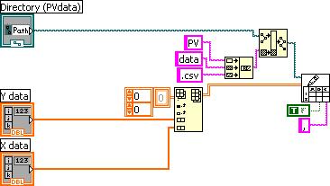
137 recordpvdata.vi: tankvalue1.vi: Write_to_csvfile.vi: test_pressures_vi.vi: 14

138 (write to specific text file) 15