Partial Differential Equation Toolbox User s Guide. R2013a

Transcription

1 Partial Differential Equation Toolbox User s Guide R2013a

2 How to Contact MathWorks Web comp.soft-sys.matlab Newsgroup Technical Support (Phone) (Fax) The MathWorks, Inc. 3 Apple Hill Drive Natick, MA Product enhancement suggestions Bug reports Documentation error reports Order status, license renewals, passcodes Sales, pricing, and general information For contact information about worldwide offices, see the MathWorks Web site. Partial Differential Equation Toolbox User s Guide COPYRIGHT The MathWorks, Inc. The software described in this document is furnished under a license agreement. The software may be used or copied only under the terms of the license agreement. No part of this manual may be photocopied or reproduced in any form without prior written consent from The MathWorks, Inc. FEDERAL ACQUISITION: This provision applies to all acquisitions of the Program and Documentation by, for, or through the federal government of the United States. By accepting delivery of the Program or Documentation, the government hereby agrees that this software or documentation qualifies as commercial computer software or commercial computer software documentation as such terms are used or defined in FAR , DFARS Part , and DFARS Accordingly, the terms and conditions of this Agreement and only those rights specified in this Agreement, shall pertain to and govern theuse,modification,reproduction,release,performance,display,anddisclosureoftheprogramand Documentation by the federal government (or other entity acquiring for or through the federal government) and shall supersede any conflicting contractual terms or conditions. If this License fails to meet the government s needs or is inconsistent in any respect with federal procurement law, the government agrees to return the Program and Documentation, unused, to The MathWorks, Inc. Trademarks MATLAB and Simulink are registered trademarks of The MathWorks, Inc. See for a list of additional trademarks. Other product or brand names may be trademarks or registered trademarks of their respective holders. Patents MathWorks products are protected by one or more U.S. patents. Please see for more information.

3 Revision History August 1995 First printing New for Version 1.0 February 1996 Second printing Revised for Version July 2002 Online only Revised for Version (Release 13) September 2002 Third printing Minor Revision for Version June 2004 Online only Revised for Version (Release 14) October 2004 Online only Revised for Version (Release 14SP1) March 2005 Online only Revised for Version (Release 14SP2) August 2005 Fourth printing Minor Revision for Version September 2005 Online only Revised for Version (Release 14SP3) March 2006 Online only Revised for Version (Release 2006a) March 2007 Online only Revised for Version (Release 2007a) September 2007 Online only Revised for Version (Release 2007b) March 2008 Online only Revised for Version (Release 2008a) October 2008 Online only Revised for Version (Release 2008b) March 2009 Online only Revised for Version (Release 2009a) September 2009 Online only Revised for Version (Release 2009b) March 2010 Online only Revised for Version (Release 2010a) September 2010 Online only Revised for Version (Release 2010b) April 2011 Online only Revised for Version (Release 2011a) September 2011 Online only Revised for Version (Release 2011b) March 2012 Online only Revised for Version (Release 2012a) September 2012 Online only Revised for Version 1.1 (Release 2012b) March 2013 Online only Revised for Version 1.2 (Release 2013a)

4

5 Contents 1 Getting Started Product Description Key Features Prerequisite Knowledge for Using This Toolbox Types of PDE Problems You Can Solve Common Toolbox Applications Typical Steps to Solve PDEs Visualize and Animate Solutions Poisson s Equation with Complex 2-D Geometry PDE Toolbox GUI Shortcuts Solving 3-D Problems Using 2-D Models Finite Element Method (FEM) Basics Setting Up Your PDE Open the PDE Toolbox GUI SpecifyGeometryUsingaCSGModel v

6 Select Graphical Objects Representing Your Geometry Rounded Corners Using CSG Modeling Enter Parameter Values as MATLAB Expressions Systems of PDEs Scalar PDE Coefficients Scalar PDE Coefficients in String Form Coefficients for Scalar PDEs in pdetool Scalar PDE Coefficients in Function Form Coefficients as the Result of a Program Calculate Coefficients in Function Form Scalar PDE Functional Form and Calling Syntax Enter Coefficients in pdetool Coefficients for Systems of PDEs D Systems in pdetool fforsystems cforsystems c as Tensor, Matrix, and Vector Scalar c Two-Element Column Vector c Three-Element Column Vector c Four-Element Column Vector c N-Element Column Vector c N-Element Column Vector c N-Element Column Vector c vi Contents

7 4N-Element Column Vector c N(2N+1)/2-Element Column Vector c N 2 -Element Column Vector c aordforsystems Coefficients a or d Scalar a or d N-Element Column Vector a or d N(N+1)/2-Element Column Vector a or d N 2 -Element Column Vector a or d Initial Conditions Types of Boundary Conditions No Boundary Conditions Between Subdomains Identify Boundary Labels Boundary Conditions Overview Boundary Conditions for Scalar PDE Boundary Conditions for PDE Systems Tooltip Displays for Mesh and Plots Mesh Data Adaptive Mesh Refinement Improving Solution Accuracy Using Mesh Refinement ErrorEstimatefortheFEMSolution Mesh Refinement Functions Mesh Refinement Termination Criteria vii

8 3 Solving PDEs Set Up and Solve Your PDE Problem Structural Mechanics Plane Stress Example Using the Graphical User Interface Structural Mechanics Plane Strain Clamped, Square Isotropic Plate With a Uniform Pressure Load Deflection of a Piezoelectric Actuator Electrostatics Example Using the Graphical User Interface Magnetostatics Example Using the Graphical User Interface AC Power Electromagnetics Example Using the Graphical User Interface Conductive Media DC Example Heat Transfer Example Using the Graphical User Interface Nonlinear Heat Transfer In a Thin Plate Diffusion viii Contents

9 Elliptic PDEs Solve Poisson s Equation on a Unit Disk Scattering Problem Minimal Surface Problem Domain Decomposition Problem Parabolic PDEs Heat Equation for Metal Block with Cavity Heat Distribution in a Radioactive Rod Hyperbolic PDEs Wave Equation Eigenvalue Problems Eigenvalues and Eigenfunctions for the L-Shaped Membrane L-Shaped Membrane with a Rounded Corner Eigenvalues and Eigenmodes of a Square Solve PDEs Programmatically When You Need Programmatic Solutions Data Structures in Partial Differential Equation Toolbox Tips for Solving PDEs Programmatically Solve Poisson s Equation on a Grid Graphical User Interface PDE Toolbox GUI Menus File Menu New Open Save As Export Image Print ix

10 Edit Menu Paste Options Menu Grid Spacing Axes Limits Application Draw Menu Rotate Boundary Menu Specify Boundary Conditions in pdetool PDE Menu PDE Specification in pdetool Mesh Menu Parameters Solve Menu Parameters Plot Menu Parameters Window Menu Help Menu Finite Element Method Elliptic Equations Systems of PDEs x Contents

11 Parabolic Equations Reducing Parabolic Equations to Elliptic Equations Solve a Parabolic Equation Hyperbolic Equations Eigenvalue Equations Nonlinear Equations References Functions Alphabetical List Index xi

12 xii Contents

13 1 Getting Started Product Description on page 1-2 Prerequisite Knowledge for Using This Toolbox on page 1-3 Types of PDE Problems You Can Solve on page 1-4 Common Toolbox Applications on page 1-7 Typical Steps to Solve PDEs on page 1-9 Visualize and Animate Solutions on page 1-11 Poisson s Equation with Complex 2-D Geometry on page 1-12 PDE Toolbox GUI Shortcuts on page 1-28 Solving 3-D Problems Using 2-D Models on page 1-31 Finite Element Method (FEM) Basics on page 1-32

14 1 Getting Started Product Description Solve partial differential equations using finite element methods The Partial Differential Equation Toolbox product contains tools for the study and solution of partial differential equations (PDEs) in two-space dimensions (2-D) and time. A set of command-line functions and a graphical user interface let you preprocess, solve, and postprocess generic 2-D PDEs for a broad range of engineering and science applications. Key Features Complete GUI for pre- and post-processing 2-D PDEs Automatic and adaptive meshing Geometry creation using constructive solid geometry (CSG) paradigm Boundary condition specification: Dirichlet, generalized Neumann, and mixed Flexible coefficient and PDE problem specification using MATLAB syntax Fully automated mesh generation and refinement Nonlinear and adaptive solvers handle systems with multiple dependent variables Simultaneous visualization of multiple solution properties, FEM-mesh overlays, and animation 1-2

15 Prerequisite Knowledge for Using This Toolbox Prerequisite Knowledge for Using This Toolbox Partial Differential Equation Toolbox software is designed for both beginners and advanced users. The minimal requirement is that you can formulate a PDE problem on paper (draw the domain, write the boundary conditions, and the PDE). At the MATLAB command line, type pdetool This invokes the graphical user interface (GUI), which is a self-contained graphical environment for PDE solving. For common applications you can use the specific physical terms rather than abstract coefficients. Using pdetool requires no knowledge of the mathematics behind the PDE, the numerical schemes, or MATLAB. Poisson s Equation with Complex 2-D Geometry on page 1-12 guides you through an example step by step. Advanced applications are also possible by downloading the domain geometry, boundary conditions, and mesh description to the MATLAB workspace. You can use functions to, for example, generate meshes, discretize your problem, interpolate, and plot data on unstructured grids. 1-3

16 1 Getting Started Types of PDE Problems You Can Solve This toolbox applies to the following PDE type: cuau f, expressed in Ω, which we shall refer to as the elliptic equation, regardlessof whether its coefficients and boundary conditions make the PDE problem elliptic in the mathematical sense. Analogously, we shall use the terms parabolic equation and hyperbolic equation for equations with spatial operators like the previous one, and first and second order time derivatives, respectively. Ω is a bounded domain in the plane. c, a, f, and the unknown u are scalar, complex valued functions defined on Ω. c can be a 2-by-2 matrix function on Ω. The software can also handle the parabolic PDE u d cuau f, t the hyperbolic PDE 2 d u cuau f, 2 t and the eigenvalue problem cuau du, where d is a complex valued function on Ω, andλ is an unknown eigenvalue. For the parabolic and hyperbolic PDE the coefficients c, a, f, andd can depend on time, on the solution u, andonitsgradient u. A nonlinear solver (pdenonlin) is available for the nonlinear elliptic PDE cu ( ) uauu ( ) f( u), where c, a, andf are functions of the unknown solution u and on its gradient u. The parabolic and hyperbolic equation solvers also solve nonlinear and time-dependent problems. 1-4

17 Types of PDE Problems You Can Solve Note Before solving a nonlinear elliptic PDE, from the Solve menu in the pdetool GUI, select Parameters. Then,selecttheUse nonlinear solver check box and click OK. All solvers can handle the system case of N coupled equations. You can solve N = 1 or 2 equations using pdetool, and any number of equations using command-line functions. For example, N = 2 elliptic equations: c u c u a u a u f c21u1 c22u2 a u a u f For a description of N > 1 PDE systems and their coefficients, see Coefficients for Systems of PDEs on page For the elliptic problem, an adaptive mesh refinement algorithm is implemented. It can also be used in conjunction with the nonlinear solver. In addition, a fast solver for Poisson s equation on a rectangular grid is available. The following boundary conditions are defined for scalar u: Dirichlet: hu = r on the boundary Ω. Generalized Neumann: n cuqu g on Ω. n is the outward unit normal. g, q, h, andr are complex-valued functions defined on Ω. (The eigenvalue problem is a homogeneous problem, i.e., g= 0, r = 0.) In the nonlinear case, the coefficients g, q, h, andr can depend on u, and for the hyperbolic and parabolic PDE, the coefficients can depend on time. For the two-dimensional system case, Dirichlet boundary condition is h11u1 h12u2 r1 h u h u r, the generalized Neumann boundary condition is 1-5

18 1 Getting Started n c11u1 n c12u2 q11u1 q12u2 g1 n c u n c u q u q u g and the mixed boundary condition is h11u1 h12u2 r1 n c11u1 n c12u2 q11u1 q12u2 g1 h11 n c u n c u q u q u g h, where µ is computed such that the Dirichlet boundary condition is satisfied. Dirichlet boundary conditions are also called essential boundary conditions, and Neumann boundary conditions are also called natural boundary conditions. For advanced, nonstandard applications you can transfer the description of domains, boundary conditions etc. to your MATLAB workspace. From there you use Partial Differential Equation Toolbox functions for managing data on unstructured meshes. You have full access to the mesh generators, FEM discretizations of the PDE and boundary conditions, interpolation functions, etc. You can design your own solvers or use FEM to solve subproblems of more complex algorithms. See also Solve PDEs Programmatically on page

19 Common Toolbox Applications Common Toolbox Applications Elliptic and parabolic equations are used for modeling: Steady and unsteady heat transfer in solids Flows in porous media and diffusion problems Electrostatics of dielectric and conductive media Potential flow Steady state of wave equations Hyperbolic equation is used for: Transient and harmonicwavepropagationinacousticsand electromagnetics Transverse motions of membranes Eigenvalue problems are used for: Determining natural vibration states in membranes and structural mechanics problems In addition to solving generic scalar PDEs and generic systems of PDEs with vector valued u, Partial Differential Equation Toolbox provides tools for solving PDEs that occur in these common applications in engineering and science: Structural Mechanics Plane Stress on page 3-6 Structural Mechanics Plane Strain on page 3-13 Electrostatics on page 3-33 Magnetostatics on page 3-36 AC Power Electromagnetics on page 3-43 Conductive Media DC on page 3-49 Heat Transfer on page 3-56 Diffusion on page

20 1 Getting Started The PDE Toolbox GUI lets you specify PDE coefficients and boundary conditions in terms of physical entities. For example, you can specifyyoung s modulus in structural mechanics problems. The application mode can be selected directly from the pop-up menu in theupperrightpartoftheguiorbyselectinganapplicationfromthe Application submenuintheoptions menu. Changing the application resets all PDE coefficients and boundary conditions to the default values for that specific application mode. When using an application mode, the generic PDE coefficients are replaced by application-specific parameters such as Young s modulus for problems in structural mechanics. The application-specific parameters are entered by selecting Parameters from the PDE menu or by clicking the PDE button. You can also access the PDE parameters by double-clicking a subdomain, if youareinthepdemode.thatwayitispossibletodefinepdeparameters for problems with regions of different material properties. The Boundary condition dialog box is also altered so that the Description column reflects the physical meaning of the different boundary condition coefficients. Finally, the Plot Selection dialog box allows you to visualize the relevant physical variables for the selected application. Note In the User entry options in the Plot Selection dialog box, the solution and its derivatives are always referred to as u, ux, anduy (v, vx, andvy for the system cases) even if the application mode is nongeneric and the solution of the application-specific PDE normally is named, e.g., V or T. The PDE Toolbox GUI lets you solve problems with vector valued u of dimension two. However, you can use functions to solve problems for any dimension of u. 1-8

21 Typical Steps to Solve PDEs Typical Steps to Solve PDEs Partial Differential Equation Toolbox provides the PDE Toolbox GUI that you can use to: 1 Define the 2-D geometry. You create Ω, the geometry, using the constructive solid geometry (CSG) model paradigm. A set of solid objects (rectangle, circle, ellipse, and polygon) is provided. You can combine these objects using set formulas. 2 Define the boundary conditions. You can have different types of boundary conditions on different boundary segments. See Types of Boundary Conditions on page Define the PDE coefficients. See Scalar PDE Coefficients on page 2-14 and Coefficients for Systems of PDEs on page You interactively specify the type of PDE and the coefficients c, a, f, andd. You can specify the coefficients for each subdomain independently. This may ease the specification of, e.g., various material properties in a PDE model. 4 Create the triangular mesh. Generate the mesh to a fineness that adequately resolves the important features in the geometry, but is coarse enough to run in a reasonable amount of time and memory. 5 Solve the PDE. You can invoke and control the nonlinear and adaptive solvers for elliptic problems. For parabolic and hyperbolic problems, you can specify the initial values, and the times for which the output should be generated. For the eigenvalue solver, you can specify the interval in which to search for eigenvalues. 6 Plot the solution and other physical properties calculated from the solution (post processing). 1-9

22 1 Getting Started After solving a problem, you can return to the mesh mode to further refine your mesh and then solve again. You can also employ the adaptive mesh refiner and solver, adaptmesh. This option tries to find a mesh that fits the solution. 1-10

23 Visualize and Animate Solutions Visualize and Animate Solutions From the graphical user interface you can use plot mode, where you have a wide range of visualization possibilities. You can visualize both inside the pdetool GUI and in separate figures. You can plot three different solution properties at the same time, using color, height, and vector field plots. Surface, mesh, contour, and arrow (quiver) plots are available. For surface plots, you can choose between interpolated and flat rendering schemes. The mesh may be hidden or exposed in all plot types. For parabolic and hyperbolic equations, you can even produce an animated movie of the solution s time dependence. All visualization functions are also accessible from the command line. 1-11

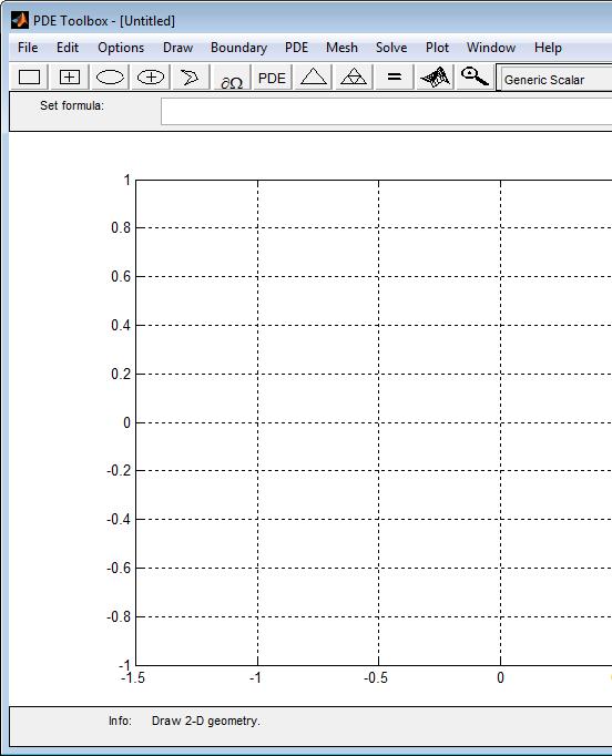
24 1 Getting Started Poisson s Equation with Complex 2-D Geometry This example shows how to solve the Poisson s equation, Δu = f using pdetool. This problem requires configuring a 2-D geometry with Dirichlet and Neumann boundary conditions. To start the GUI, type the command pdetool at the MATLAB prompt. The GUI looks similar to the following figure, with exception of the grid. Turn on the grid by selecting Grid from the Options menu. Also, enable the snap-to-grid feature by selecting Snap from the Options menu. The snap-to-grid feature simplifies aligning the solid objects. 1-12

25 Poisson sequationwithcomplex2-dgeometry 1-13

26 1 Getting Started ThefirststepistodrawthegeometryonwhichyouwanttosolvethePDE. The GUI provides four basic types of solid objects: polygons, rectangles, circles, and ellipses. The objects are used to create a Constructive Solid Geometry model (CSG model). Each solid object is assigned a unique label, and by the use of set algebra, the resulting geometry can be made up of a combination of unions, intersections, and set differences. By default, the resulting CSG model is the union of all solid objects. To select a solid object, either click the button with an icon depicting the solid object that you want to use, or select the object by using the Draw pull-down menu. In this case, rectangle/square objects are selected. To draw a rectangle or a square starting at a corner, click the rectangle button without a + sign in the middle. The button with the + sign is used when you want to draw starting at the center. Then, put the cursor at the desired corner, and click-and-drag using the left mouse button to create a rectangle with the desired side lengths. (Use the right mouse button to create a square.) Click and drag from ( 1,.2) to (1,.2). Notice how the snap-to-grid feature forces the rectangle to line up with the grid. When you release the mouse, the CSG model is updated and redrawn. At this stage, all you have is a rectangle. It is assignedthelabelr1. Ifyouwanttomoveorresizetherectangle,youcan easily do so. Click-and-drag an object to move it, and double-click an object to open a dialog box, where you can enter exact location coordinates. From the dialog box, you can also alter the label. If you are not satisfied and want to restart, you can delete the rectangle by clicking the Delete key or by selecting Clear from the Edit menu. Next, draw a circle by clicking the button with the ellipse icon with the + sign, and then click-and-drag in a similar way, starting near the point (.5,0) with radius.4, using the right mouse button, starting at the circle center. 1-14

27 Poisson sequationwithcomplex2-dgeometry 1-15

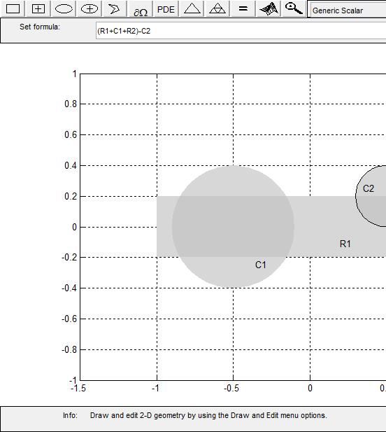
28 1 Getting Started The resulting CSG model is the union of the rectangle R1 and the circle C1, described by set algebra as R1+C1. The area where the two objects overlap is clearly visible as it is drawn using a darker shade of gray. The object that you just drew the circle has a black border, indicating that it is selected. A selected object can be moved, resized, copied, and deleted. You can select more than one object by Shift+clicking the objects that you want to select. Also, a Select All option is available from the Edit menu. Finally, add two more objects, a rectangle R2 from (.5,.6) to (1,1), and a circle C2 centered at (.5,.2) with radius.2. The desired CSG model is formed by subtracting the circle C2 from the union of the other three objects. You do this by editing the set formula that by default is the union of all objects: C1+R1+R2+C2. You can type any other valid set formula into Set formula edit field. Click in the edit field and use the keyboard to change the set formula to (R1+C1+R2)-C2 1-16

29 Poisson sequationwithcomplex2-dgeometry 1-17

30 1 Getting Started If you want, you can save this CSG model as a file. Use the Save As option from the File menu, and enter a filename of your choice. It is good practice to continue to save your model at regular intervals using Save. All the additional steps in the process of modeling and solving your PDE are then saved to the same file. This concludes the drawing part. You can now define the boundary conditions for the outer boundaries. Enter theboundarymodebyclickingthe Ω icon or by selecting Boundary Mode from the Boundary menu. You can now remove subdomain borders and define the boundary conditions. The gray edge segments are subdomain borders induced by the intersections of the original solid objects. Borders that do not represent borders between, e.g., areas with differing material properties, can be removed. From the Boundary menu, select the Remove All Subdomain Borders option. All borders are then removed from the decomposed geometry. The boundaries are indicated by colored lines with arrows. The color reflects the type of boundary condition, and the arrow points toward the end of the boundary segment. The direction information is provided for the case when the boundary condition is parameterized along the boundary. The boundary condition can also be a function of x and y, or simply a constant. By default, the boundary condition is of Dirichlet type: u =0ontheboundary. Dirichlet boundary conditions are indicated by red color. The boundary conditions can also be of a generalized Neumann (blue) or mixed (green) type. For scalar u, however, all boundary conditions are either of Dirichlet or the generalized Neumann type. You select the boundary conditions that you want to change by clicking to select one boundary segment, by Shift+clicking to select multiple segments, or by using the Edit menu option Select All to select all boundary segments. The selected boundary segments are indicated by black color. For this problem, change the boundary condition for all the circle arcs. Select them by using the mouse and Shift+click those boundary segments. 1-18

31 Poisson sequationwithcomplex2-dgeometry 1-19

32 1 Getting Started Double-clicking anywhere on the selected boundary segments opens the Boundary Condition dialog box. Here, you select the type of boundary condition, and enter the boundary condition as a MATLAB expression. Change the boundary condition along the selected boundaries to a Neumann condition, u/ n = 5. This means that the solution has a slope of 5 in the normal direction for these boundary segments. In the Boundary Condition dialog box, select the Neumann condition type, and enter -5 in the edit box for the boundary condition parameter g. Todefine a pure Neumann condition, leave the q parameter at its default value, 0. When you click the OK button, notice how the selected boundary segments change to blue to indicate Neumann boundary condition. Next, specify the PDE itself through a dialog box that is accessed by clicking the button with the PDE icon or by selecting PDE Specification from the PDE menu. In PDE mode, you can also access the PDE Specification dialog box by double-clicking a subdomain. That way, different subdomains can have different PDE coefficient values. This problem, however, consists of only one subdomain. 1-20

33 Poisson sequationwithcomplex2-dgeometry In the dialog box, you can select the type of PDE (elliptic, parabolic, hyperbolic, or eigenmodes) and define the applicable coefficients depending on the PDE type. This problem consists of an elliptic PDE defined by the equation cuau f, with c =1.0,a =0.0,andf = Finally, create the triangular mesh that Partial Differential Equation Toolbox software uses in the Finite Element Method (FEM) to solve the PDE. The triangular mesh is created and displayed when clicking the button with the icon or by selecting the Mesh menu option Initialize Mesh. Ifyouwant amore accurate solution, the mesh can be successively refined by clicking the buttonwiththefourtriangleicon(therefine button) or by selecting the Refine Mesh option from the Mesh menu. Using the Jiggle Mesh option, the mesh can be jiggled to improve the triangle quality. Parameters for controlling the jiggling of the mesh, the refinement method, and other mesh generation parameters can be found in adialog box that is opened by selecting Parameters from the Mesh menu. 1-21

34 1 Getting Started You can undo any change to the mesh by selecting the Mesh menu option Undo Mesh Change. Initialize the mesh, then refine it once and finally jiggle it once. 1-22

35 Poisson sequationwithcomplex2-dgeometry 1-23

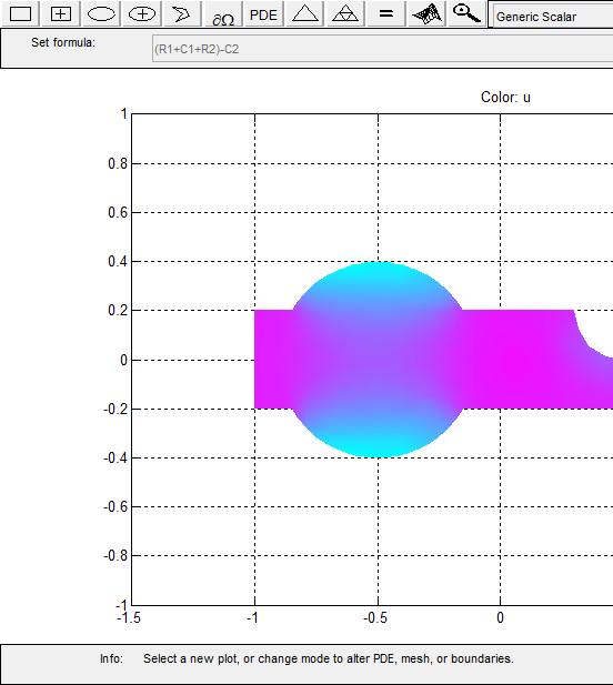
36 1 Getting Started We are now ready to solve the problem. Click the = button or select Solve PDE from the Solve menu to solve the PDE. The solution is then plotted. By default, the plot uses interpolated coloring and a linear color map. A color bar is also provided to map the different shades to the numerical values of the solution. If you want, the solution can be exported as a vector to the MATLAB main workspace. 1-24

37 Poisson sequationwithcomplex2-dgeometry 1-25

38 1 Getting Started Therearemanymoreplotmodesavailabletohelpyouvisualizethesolution. Click the button with the 3-D solution icon or select Parameters from the Plot menu to access the dialog box for selection of the different plot options. Several plot styles are available, and the solution can be plotted in the GUI or in a separate figure as a 3-D plot. Now, select a plot where the color and the height both represent u. Choose interpolated shading and use the continuous (interpolated) height option. The default colormap is the cool colormap; a pop-up menu lets you select from anumber of different colormaps. Finally, click the Plot button to plot the solution; click the Close button to save the plot setup as the current default. The solution is plotted as a 3-D plot in a separate figure window. 1-26

39 Poisson sequationwithcomplex2-dgeometry Thefollowingsolutionplotistheresult. Youcanusethemousetorotate the plot in 3-D. By clicking-and-dragging the axes, the angle from which the solution is viewed can be changed. 1-27

40 1 Getting Started PDE Toolbox GUI Shortcuts PDE Toolbox GUI toolbar provide quick access to key operations that are also available in the menus. The toolbar consists of three different parts: the five leftmost buttons for draw mode functions, the next six buttons for different boundary, mesh, solution, and plot functions, and the rightmost button for activating the zoom feature. Five buttons on the left let you draw the geometry. Double-click a button makes it stick, and you can then continue to draw solid objects of the selected type until you single-click the button to release it. In draw mode, you can create the 2-D geometry using the constructive solid geometry (CSG) model paradigm. A set of solid objects (rectangle, circle, ellipse, and polygon) is provided. These objects can be combined using set formulas in a flexible way. Draw a rectangle/square starting at a corner. Using the left mouse button, click-and-drag to create a rectangle. Using the right mouse button (or Ctrl+click), click-and-drag to create a square. Draw a rectangle/square starting at the center. Using the left mouse button, click-and-drag to create a rectangle. Using the right mouse button (or Ctrl+click), click-and-drag to create a square. Draw an ellipse/circle starting at the perimeter. Using the left mouse button, click-and-drag to create an ellipse. Using the right mouse button (or Ctrl+click), click-and-drag to create a circle. 1-28

41 PDE Toolbox GUI Shortcuts Draw an ellipse/circle starting at the center. Using the left mouse button, click-and-drag to create an ellipse. Using the right mouse button (or Ctrl+click), click-and-drag to create a circle. Draw a polygon. Click-and-drag to create polygon edges. You can close the polygon by pressing the right mouse button. Clicking at the starting vertex also closes the polygon. The remaining buttons represent, from left to right: Enters the boundary mode. In boundary mode, you can specify the boundary conditions. You can have different types of boundary conditions on different boundaries. In this mode, the original shapes of the solid objects constitute borders between subdomains of the model. Such borders can be eliminated in this mode. Opens the PDE Specification dialog box. In PDE mode, you can interactively specify the type of PDE problem, and the PDE coefficients. You can specify the coefficients for each subdomain independently. This makes it easy to specify, e.g., various material properties in a PDE model. Initializes the triangular mesh In mesh mode, you can control the automated mesh generation and plot the mesh. Refines the triangular mesh. Solves the PDE. In solve mode, you can invoke and control the nonlinear and adaptive solver for elliptic problems. For parabolic and hyperbolic PDE problems, you can specify the initial values, and the times for which the output should be generated. For the eigenvalue solver, you can specify the interval in which to search for eigenvalues. 1-29

42 1 Getting Started 3-D solution opens the Plot Selection dialog box. In plot mode, there is a wide range of visualization possibilities. You can visualize both in the pdetool GUI and in a separate figure window. You can visualize three different solution properties at the same time, using color, height, and vector field plots. There are surface, mesh, contour, and arrow (quiver) plots available. For parabolic and hyperbolic equations, you can animate the solution as it changes with time. Toggles zoom. 1-30

43 Solving 3-D Problems Using 2-D Models Solving 3-D Problems Using 2-D Models Partial Differential Equation Toolbox software solves problems in two space dimensions and time, whereas reality has three space dimensions. The reductionto2-dispossiblewhenvariationsinthethirdspacedimension (taken to be z) can be accounted for in the 2-D equation. In some cases, like the plane stress analysis, the material parameters must be modified in the process of dimensionality reduction. When the problem is such that variation with z is negligible, all z-derivatives drop out and the 2-D equation has exactly the same units and coefficients as in 3-D. Slab geometries are treated by integration through the thickness. The result is a 2-D equation for the z-averagedsolutionwiththethickness,sayd(x,y), multiplied onto all the PDE coefficients, c, a, d, andf, etc. Forinstance,if you want to compute the stresses in a sheet welded together from plates of different thickness, multiply Young s modulus E, volume forces, and specified surface tractions by D(x,y), Similar definitions of the equation coefficients are called for in other slab geometry examples and application modes. 1-31

44 1 Getting Started Finite Element Method (FEM) Basics The core Partial Differential Equation Toolbox algorithm is a PDE solver that uses the Finite Element Method (FEM) for problems defined on bounded domains in the plane. The solutions of simple PDEs on complicated geometries can rarely be expressed in terms of elementary functions. You are confronted with two problems: First you need to describe a complicated geometry and generate ameshonit. ThenyouneedtodiscretizeyourPDEonthemeshandbuild an equation for the discrete approximation of the solution. The pdetool graphical user interface provides you with easy-to-use graphical tools to describe complicated domains and generate triangular meshes. It also discretizes PDEs, finds discrete solutions and plots results. You can access the mesh structures and the discretization functions directly from the command line (or from a file) and incorporate them into specialized applications. Here is an overview of the Finite Element Method (FEM). The purpose of this presentation is to get you acquainted with the elementary FEM notions. Here you find the precise equations that are solved and the nature of the discrete solution. Different extensions of the basic equation implemented in Partial Differential Equation Toolbox software are presented. A more detailed description can be found in Elliptic Equations on page 5-2, with variants for specific types in Systems of PDEs on page 5-10, Parabolic Equations on page 5-13, Hyperbolic Equations on page 5-18, Eigenvalue Equations on page 5-19, and Nonlinear Equations on page You start by approximating the computational domain Ω with a union of simple geometric objects, in this case triangles. The triangles form a mesh and each vertex is called a node. You are in the situation of an architect designing a dome. He has to strike a balance between the ideal rounded forms of the original sketch and the limitations of his simple building-blocks, triangles or quadrilaterals. If the result does not look close enough to a perfect dome, the architect can always improve his work using smaller blocks. Next you say that your solution should be simple on each triangle. Polynomials are a good choice: they are easy to evaluate and have good approximation properties on small domains. You can ask that the solutions in neighboring triangles connect to each other continuously across the edges. You can still decide how complicated the polynomials can be. Just like an 1-32

45 Finite Element Method (FEM) Basics architect,youwantthemassimpleaspossible. Constantsarethesimplest choice but you cannot match values on neighboring triangles. Linear functions come next. This is like using flat tiles to build a waterproof dome, which is perfectly possible. A Triangular Mesh (left) and a Continuous Piecewise Linear Function on That Mesh Now you use the basic elliptic equation (expressed in Ω) cuau f, If u h is the piecewise linear approximation to u, it is not clear what the second derivative term means. Inside each triangle, u h is a constant (because u h is flat) and thus the second-order term vanishes. At the edges of the triangles, c u h is in general discontinuous and a further derivative makes no sense. What you are looking for is the best approximation of u in the class of continuous piecewise polynomials. Therefore you test the equation for u h against all possible functions v of that class. Testing means formally to multiply the residual against any function and then integrate, i.e., determine u h such that 1-33

46 1 Getting Started cuhauh fvdx 0 for all possible v. The functions v are usually called test functions. Partial integration (Green s formula) yields that u h should satisfy cu v au v dx n c u v ds fv dx v, h h h where Ω is the boundary of Ω and n is the outward pointing normal on Ω. The integrals of this formulation are well-defined even if u h and v are piecewise linear functions. Boundary conditions are included in the following way. If u h is known at some boundary points (Dirichlet boundary conditions), we restrict the test functions to v = 0 at those points, and require u h to attain the desired value at that point. At all the other points we ask for Neumann boundary conditions, i.e., ( c uh) n+ quh = g. The FEM formulation reads: Find u h such that (( c u ) v+ au v) dx+ qu vds = fvdx+ gvds v, Ω h h Ω h Ω Ω 1 1 where Ω 1 is the part of the boundary with Neumann conditions. The test functions v must be zero on Ω Ω 1. Any continuous piecewise linear u h is represented as a combination N uh( x) Ui i( x), i1 where ϕ i aresomespecialpiecewiselinearbasisfunctionsandu i are scalar coefficients. Choose ϕ i like a tent, such that it has the height 1 at the node i and the height 0 at all other nodes. For any fixed v, the FEM formulation yields an algebraic equation in the unknowns U i. You want to determine N unknowns, so you need N different instances of v. What better candidates than v = ϕ i, i =1,2,...,N? YoufindalinearsystemKU = F where the matrix 1-34

47 Finite Element Method (FEM) Basics K and the right side F contain integrals in terms of the test functions ϕ i, ϕ j, and the coefficients defining the problem: c, a, f, q, andg. Thesolutionvector U contains the expansion coefficients of u h,whicharealsothevaluesofu h at each node x i,sinceu h (x i )=U i. If the exact solution u is smooth, then FEM computes u h with an error of the same size as that of the linear interpolation. It is possible to estimate the error on each triangle using only u h and the PDE coefficients (but not the exact solution u, which in general is unknown). There are Partial Differential Equation Toolbox functions that assemble K and F. This is done automatically in the graphical user interface, but you also have direct access to the FEM matrices from the command-line function assempde. To summarize, the FEM approach is to approximate the PDE solution u by a piecewise linear function u h. The function u h is expanded in a basis of test-functions ϕ i, and the residual is tested against all the basis functions. This procedure yields a linear system KU = F. The components of U are the values of u h at the nodes. For x inside a triangle, u h (x) is found by linear interpolation from the nodal values. FEM techniques are also used to solve more general problems. The following are some generalizations that you can access both through the graphical user interface and with command-line functions. Time-dependent problems are easy to implement in the FEM context. The solution u(x,t) of the equation u d cuau f, t can be approximated by N u ( x, t) U ( t) ( x). h i i i1 This yields a system of ordinary differential equations (ODE) 1-35

48 1 Getting Started M du dt KU F, which you integrate using ODE solvers. Two time derivatives yield a second order ODE 2 M du KU F 2 dt, etc. The toolbox supports problems with one or two time derivatives (the functions parabolic and hyperbolic). Eigenvalue problems: Solve cuau du, for the unknowns u and λ (λ is a complex number). Using the FEM discretization, you solve the algebraic eigenvalue problem KU = λ h MU to find u h and λ h as approximations to u and λ. A robust eigenvalue solver is implemented in pdeeig. If the coefficients c, a, f, q, org are functions of u or u, thepdeiscalled nonlinear and FEM yields a nonlinear system K(U)U = F(U). You can use iterative methods for solving the nonlinear system. For elliptic equations, the toolbox provides a nonlinear solver called pdenonlin using a damped Gauss-Newton method. The parabolic and hyperbolic functions call the nonlinear solver automatically. Small triangles are needed only in those parts of the computational domain where the error is large. In many cases the errors are large in a small region and making all triangles small is a waste of computational effort. Making small triangles only where needed is called adapting the mesh refinement to the solution. An iterative adaptive strategy is the following: For a given mesh, form and solve the linear system KU = F. Thenestimate the error and refine the triangles in which the error is large. The iteration is controlled by adaptmesh and the error is estimated by pdejmps. Although the basic equation is scalar, systems of equations are also handled by the toolbox. The interactive environment accepts u asascalaror2-vector function. In command-line mode, systems of arbitrary size are accepted. 1-36

49 Finite Element Method (FEM) Basics If c δ >0anda 0, under rather general assumptions on the domain Ω and the boundary conditions, the solution u exists and is unique. The FEM linear system has a unique solution which converges to u as the triangles become smaller. The matrix K and the right side F make sense even when u does not exist or is not unique. It is advisable that you devise checks to problems with questionable solutions. References [1] Cook, Robert D., David S. Malkus, and Michael E. Plesha, Concepts and Applications of Finite Element Analysis, 3rd edition, John Wiley & Sons, New York,

50 1 Getting Started 1-38

51 2 Setting Up Your PDE Open the PDE Toolbox GUI on page 2-3 Specify Geometry Using a CSG Model on page 2-5 Select Graphical Objects Representing Your Geometry on page 2-7 Rounded Corners Using CSG Modeling on page 2-8 Enter Parameter Values as MATLAB Expressions on page 2-12 Systems of PDEs on page 2-13 Scalar PDE Coefficients on page 2-14 Scalar PDE Coefficients in String Form on page 2-16 Coefficients for Scalar PDEs in pdetool on page 2-19 Scalar PDE Coefficients in Function Form on page 2-23 Scalar PDE Functional Form and Calling Syntax on page 2-26 Enter Coefficients in pdetool on page 2-32 Coefficients for Systems of PDEs on page D Systems in pdetool on page 2-44 f for Systems on page 2-48 c for Systems on page 2-50 a or d for Systems on page 2-59 Initial Conditions on page 2-62 Types of Boundary Conditions on page 2-64 No Boundary Conditions Between Subdomains on page 2-65 Identify Boundary Labels on page 2-68

52 2 Setting Up Your PDE Boundary Conditions Overview on page 2-70 Boundary Conditions for Scalar PDE on page 2-71 Boundary Conditions for PDE Systems on page 2-76 Tooltip Displays for Mesh and Plots on page 2-83 Mesh Data on page 2-84 Adaptive Mesh Refinement on page

53 Open the PDE Toolbox GUI Open the PDE Toolbox GUI Partial Differential Equation Toolbox software includes a complete graphical user interface (GUI), which covers all aspects of the PDE solution process. You start it by typing pdetool at the MATLAB command line. It may take a while the first time you launch pdetool during a MATLAB session. The following figure shows the pdetool GUI as it looks when you start it. At the top, the GUI has a pull-down menu bar that you use to control the modeling. Below the menu bar, a toolbar with icon buttons provide quick and easy access to some of the most important functions. To the right of the toolbar is a pop-up menu that indicates the current application mode. You can also use it to change the application mode. The upper right part of the GUI also provides the x- andy-coordinates of the 2-3

54 2 Setting Up Your PDE current cursor position. This position is updated when you move the cursor inside the main axes area in the middle of the GUI. Theeditboxforthesetformulacontains the active set formula. In the main axes you draw the 2-D geometry, display the mesh, and plot the solution. At the bottom of the GUI, an information line provides information about the current activity. It can also display help information about the toolbar buttons. 2-4

55 SpecifyGeometryUsingaCSGModel Specify Geometry Using a CSG Model You can specify complex geometries by overlapping solid objects. This approach to representing geometries is called Constructive Solid Geometry (CSG). Use these four solid objects to specify a geometry for your problem: Circle Represents the set of points inside and on a circle. Polygon Represents the set of points inside and on a polygon given by a set of line segments. Rectangle Represents the set of points inside and on a rectangle. Ellipse Represents the set of points inside and on an ellipse. The ellipse can be rotated. When you draw a solid object in the GUI, each solid object is automatically given a unique name. Default names are C1, C2, C3, etc., for circles; P1, P2, P3, etc. for polygons; R1, R2, R3, etc., for rectangles; E1, E2, E3, etc., for ellipses. Squares, although a special case of rectangles, are named SQ1, SQ2, SQ3, etc. The name is displayed on the solid object itself. You can use any unique name, as long as it contains no blanks. In draw mode, you can alter the names and the geometries of the objects by double-clicking them, which opens a dialog box. The following figure shows an object dialog box for a circle. You can use the name of the object to refer to the corresponding set of points in a set formula. The operators +, *, and are used to form the set of points Ω in the plane over which the differential equation is solved. The operators +, the set union operator, and *, the set intersection operator, have the 2-5

56 2 Setting Up Your PDE same precedence. The operator, the set difference operator, has higher precedence. The precedence can be controlled by using parentheses. The resulting geometrical model, Ω, isthesetofpointsforwhichthesetformula evaluates to true. By default, it is the union of all solid objects. We often refer to the area Ω as the decomposed geometry. 2-6

57 Select Graphical Objects Representing Your Geometry Select Graphical Objects Representing Your Geometry Throughout the GUI, similar principles apply for selecting objects such as solid objects, subdomains, and boundaries. To select a single object, click it usingtheleftmousebutton. To select several objects and to deselect objects, Shift+click (or click using themiddlemousebutton)onthedesiredobjects. Clicking in the intersection of several objects selects all the intersecting objects. To open an associated dialog box, double-click an object. If the object is not selected, it is selected before opening the dialog box. In draw mode and PDE mode, clicking outside of objects deselects all objects. To select all objects, use the Select All option from the Edit menu. When defining boundary conditions and the PDE via the menu items from the Boundary and PDE menus, and no boundaries or subdomains are selected, the entered values applies to all boundaries and subdomains by default. 2-7

58 2 Setting Up Your PDE Rounded Corners Using CSG Modeling This example shows how to represent a geometry that includes rounded corners (fillets) using Constructive Solid Geometry (CSG) modeling. You learn how to draw several overlapping solid objects, and specify how these objects should combine to produce the desired geometry. Start the GUI using pdetool and turn on the grid and the snap-to-grid feature using the Options menu. Also, change the grid spacing to -1.5:0.1:1.5 for the x-axis and -1:0.1:1 for the y-axis. Select Rectangle/square from the Draw menu or click the button with the rectangleicon. Thendrawarectanglewithawidthof2andaheightof1 using the mouse, starting at ( 1,0.5). To get the round corners, add circles, one in each corner. The circles should have a radius of 0.2 and centers at a distance that is 0.2 units from the left/right and lower/upper rectangle boundaries (( 0.8, 0.3), ( 0.8,0.3), (0.8, 0.3), and (0.8,0.3)). To draw several circles, double-click the button for drawing ellipses/circles (centered). Then draw the circles using the right mouse button or Ctrl+click starting at the circle centers. Finally, at each of the rectangle corners, draw four small squares with a side of 0.2. The following figure shows the complete drawing. 2-8

59 Rounded Corners Using CSG Modeling Now you have to edit the set formula. To get the rounded corners, subtract the small squares from the rectangle and then add the circles. As a set formula, this is expressed as R1-(SQ1+SQ2+SQ3+SQ4)+C1+C2+C3+C4 2-9

60 2 Setting Up Your PDE Enter the set formula into the edit box at the top of the GUI. Then enter the Boundary mode by clicking the Ω button or by selecting the Boundary Mode option from the Boundary menu. The CSG model is now decomposed using the set formula, and you get a rectangle with rounded corners, as shown in the following figure. 2-10

61 Rounded Corners Using CSG Modeling Because of the intersection of the solid objects used in the initial CSG model, a number of subdomain borders remain. They are drawn using gray lines. If this is a model of, e.g., a homogeneous plate, you can remove them. Select the Remove All Subdomain Borders option from the Boundary menu. The subdomain borders are removed and the model of the plate is now complete. 2-11

62 2 Setting Up Your PDE Enter Parameter Values as MATLAB Expressions When entering parameter values, e.g., as a function of x and y, theentered string must be a MATLAB expression to be evaluated for x and y defined on the current mesh, i.e., x and y are MATLAB row vectors. For example, the function 4xy should be entered as 4*x.*y and not as 4*x*y, which normally is not a valid MATLAB expression. 2-12

63 Systems of PDEs Systems of PDEs As described in Types of PDE Problems You Can Solve on page 1-4, Partial Differential Equation Toolbox can solve systems of PDEs. This means you can have N coupled PDEs, with coupled boundary conditions. The solvers such as assempde and hyperbolic can solve systems of PDEs with any number N of components. Scalar PDEs are those with N = 1, meaning just one PDE. Systems of PDEs generally means N > 1. The documentation sometimes refers to systems as multidimensional PDEs or as PDEs with vector solution u. In all cases, PDE systems have a single 2-D geometry and mesh. It is only N, the number of equations, that can vary. 2-13

64 2 Setting Up Your PDE Scalar PDE Coefficients A scalar PDE is one of the following: Elliptic cuau f, Parabolic u d cuau f, t Hyperbolic 2 d u cuau f, 2 t Eigenvalue cuau du, In all cases, the coefficients d, c, a, andf can be functions of position (x and y) and the subdomain index. For all cases except eigenvalue, the coefficients can also depend on the solution u and its gradient. And for parabolic and hyperbolic equations, the coefficients can also depend on time. The question is how to represent the coefficients for the toolbox. There are three ways of representing each coefficient. You can use different ways for different coefficients. Numeric If a coefficient is numeric, give the value. String formula See Scalar PDE Coefficients in String Form on page MATLAB function See Scalar PDE Coefficients in Function Form on page

65 Scalar PDE Coefficients For an example incorporating each way to represent coefficients, see Scalar PDE Functional Form and Calling Syntax on page Note If any coefficient depends on time or on the solution u or its gradient, then that coefficient should be NaN when either time or the solution u is NaN. This is the way that solvers check to see if the equation depends on time or on the solution. 2-15

66 2 Setting Up Your PDE Scalar PDE Coefficients in String Form Write a text expression using these conventions: 'x' x-coordinate 'y' y-coordinate 'u' Solutionofequation 'ux' Derivativeofu in the x-direction 'uy' Derivativeofu in the y-direction 't' Time (parabolic and hyperbolic equations) 'sd' Subdomain number For example, you could use this string to represent a coefficient: '(x+y)./(x.^2 + y.^2 + 1) sin(t)./(1+u.^4)' Note Use.*,./, and.^ for multiplication, division, and exponentiation operations. The text expressions operate on row vectors, so the operations must make sense for row vectors. The row vectors are the values at the triangle centroids in the mesh. You can write MATLAB functions for coefficients as well as plain text expressions. For example, suppose your coefficient f is given by the file fcoeff.m: function f = fcoeff(x,y,t,sd) f = (x.*y)./(1+x.^2+y.^2); % f on subdomain 1 f = f + log(1+t); % include time r = (sd == 2); % subdomain 2 f(r) = cos(x+y); % f on subdomain 2 Represent this function in the parabolic solver, for example: u1 = parabolic(u0,tlist,b,p,e,t,c,a,'fcoeff(x,y,t,sd)',d) 2-16

67 Scalar PDE Coefficients in String Form Caution In function form, t represents triangles, and time represents time. In string form, t represents time, and triangles do not enter into the form. There is a simple way to write a text expression for multiple subdomains without using 'sd' or a function. Separate the formulas for the different subdomains with the '!' character. Generally use the same number of expressions as subdomains. However, if an expression does not depend on the subdomain number, you can give just one expression. For example, an expression for an input (a, c, f, ord) with three subdomains: '(1+x.^2)./(1+x.^2+y.^2)!(1+(x+y).^2)./(1+x.^2+y.^2)!(1+x.^2)./(1+x.^2+y. The coefficient c is a 2-by-2 matrix. You can give c in any of the following forms: Scalar or single string The software interprets c as a diagonal matrix: c 0 0 c Two-element column vector or two-row text array The software interprets c as a diagonal matrix: c() c( 2) Three-element column vector or three-row text array The software interprets c as a symmetric matrix: c() 1 c() 2 c( 2) c( 3) Four-element column vector or four-row text array The software interprets c as a full matrix: 2-17

68 2 Setting Up Your PDE c() 1 c() 3 c( 2) c( 4) For example, c as a symmetric matrix with cos(xy) on the off-diagonal terms: c = char('x.^2+y.^2',... 'cos(x.*y)',... 'u./(1+x.^2+y.^2)') To include subdomains separated by '!', includethe'!' in each row. For example, c = char('1+x.^2+y.^2!x.^2+y.^2',... 'cos(x.*y)!sin(x.*y)',... 'u./(1+x.^2+y.^2)!u.*(x.^2+y.^2)') Caution Do not include spaces in your coefficient strings in pdetool. The string parser can misinterpret a space as a vector separator, as when a MATLABvectorusesaspacetoseparateelementsofavector. For elliptic problems, when you include 'u', 'ux', or'uy', youmustuse the pdenonlin solver instead of assempde. In pdetool, select Solve > Parameters > Use nonlinear solver. Related Examples Scalar PDE Functional Form and Calling Syntax on page 2-26 Enter Coefficients in pdetool on page 2-32 Scalar PDE Coefficients in Function Form on page 2-23 Concepts Scalar PDE Coefficients on page

69 Coefficients for Scalar PDEs in pdetool Coefficients for Scalar PDEs in pdetool To enter coefficients for your PDE, select PDE > PDE Specification. Enter text expressions using these conventions: x x-coordinate y y-coordinate u Solutionofequation ux Derivativeofuin the x-direction uy Derivativeofuin the y-direction t Time (parabolic and hyperbolic equations) sd Subdomainnumber For example, you could use this expression to represent a coefficient: (x+y)./(x.^2+y.^2+1)+3+sin(t)./(1+u.^4) 2-19

70 2 Setting Up Your PDE For elliptic problems, when you include u, ux, oruy, you must use the nonlinear solver. Select Solve > Parameters > Use nonlinear solver. Note Do not use quotes or unnecessary spaces in your entries. The string parser can misinterpret a space as a vector separator, as when a MATLAB vector uses a space to separate elements of a vector. Use.*,./, and.^ for multiplication, division, and exponentiation operations. The text expressions operate on row vectors, so the operations must make sense for row vectors. The row vectors are the values at the triangle centroids in the mesh. You can write MATLAB functions for coefficients as well as plain text expressions. For example, suppose your coefficient f is given by the file fcoeff.m. function f = fcoeff(x,y,t,sd) f = (x.*y)./(1+x.^2+y.^2); % f on subdomain 1 f = f + log(1+t); % include time r = (sd == 2); % subdomain 2 f(r) = cos(x+y); % f on subdomain 2 Use fcoeff(x,y,t,sd) as the f coefficient in the parabolic solver. 2-20

71 Coefficients for Scalar PDEs in pdetool Alternatively, you can represent a coefficient in function form rather than in string form. See Scalar PDE Coefficients in Function Form on page The coefficient c is a 2-by-2 matrix. You can give 1-, 2-, 3-, or 4-element matrix expressions. Separate the expressions for elements by spaces. These expressions mean: 1-element expression: c 0 0 c 2-element expression: 3-element expression: c() c( 2) c() 1 c() 2 c( 2) c( 3) c() 1 c() 3 4-element expression: c( 2) c( 4) For example, c is a symmetric matrix with constant diagonal entries and cos(xy) as the off-diagonal terms: 1.1 cos(x.*y) 5.5 This corresponds to coefficientsfortheparabolicequation 2-21

72 2 Setting Up Your PDE u 11. cos( xy) u 10. t cos( xy) 55. Related Examples Enter Coefficients in pdetool on page 2-32 Concepts Scalar PDE Coefficients on page

73 Scalar PDE Coefficients in Function Form Scalar PDE Coefficients in Function Form In this section... CoefficientsastheResultofaProgram onpage2-23 Calculate Coefficients in Function Form on page 2-24 Coefficients as the Result of a Program Usually. the simplest way to give coefficients as the result of a program is to use a string expression as described in Scalar PDE Coefficients in String Form on page For the most detailed control over coefficients, though, you can write a function form of coefficients. A coefficient in function form has the syntax coeff = coeffunction(p,t,u,time) coeff represents any coefficient: c, a, f, ord. Your program evaluates the return coeff as a row vector of the function values at the centroids of the triangles t. For help calculating these values, see CalculateCoefficientsinFunctionForm onpage2-24. p and t are the node points and triangles of the mesh. For a description of thesedatastructures,see MeshData onpage2-84.inbrief,eachcolumn of p contains the x- andy-values of a point, and each column of t contains the indices of three points in p and the subdomain label of that triangle. u is a row vector containing the solution at the points p. u is [] if the coefficients do not depend on the solution or its derivatives. time isthetimeofthesolution,ascalar. time is [] if the coefficients do not depend on time. Caution In function form, t represents triangles, and time represents time. In string form, t represents time, and triangles do not enter into the form. 2-23

74 2 Setting Up Your PDE Pass the coefficient function to the solver as a string 'coeffunction' or as a function Inpdetool, pass the coefficient as a string coeffunction without quotes, because pdetool interprets all entries as strings. If your coefficients depend on u or time, thenwhenu or time are NaN, ensure that the corresponding coeff consist of a vector of NaN of the correct size. This signals to solvers, such as parabolic, to use a time-dependent or solution-dependent algorithm. For elliptic problems, if any coefficient depends on u or its gradient, you must use the pdenonlin solver instead of assempde. Inpdetool, selectsolve > Parameters > Use nonlinear solver. Calculate Coefficients in Function Form X- and Y-Values The x- andy-values of the centroid of a triangle t are the mean values of the entries of the points p in t. To get row vectors xpts and ypts containing the mean values: % Triangle point indices it1=t(1,:); it2=t(2,:); it3=t(3,:); % Find centroids of triangles xpts=(p(1,it1)+p(1,it2)+p(1,it3))/3; ypts=(p(2,it1)+p(2,it2)+p(2,it3))/3; Interpolated u The pdeintrp function linearly interpolates the values of u at the centroids of t, based on the values at the points p. uintrp = pdeintrp(p,t,u); % Interpolated values at centroids The output uintrp is a row vector with the same number of columns as t. Use uintrp as the solution value in your coefficient calculations. 2-24

75 Scalar PDE Coefficients in Function Form Gradient or Derivatives of u The pdegrad function approximates the gradient of u. [ux,uy] = pdegrad(p,t,u); % Approximate derivatives The outputs ux and uy are row vectors with the same number of columns as t. Subdomains If your coefficients depend on the subdomain label, check the subdomain number for each triangle. Subdomains are the last (fourth) row of the triangle matrix. So the row vector of subdomain numbers is: subd = t(4,:); You can see the subdomain labels by using the pdegplot function with the subdomainlabels name-value pair set to 'on': pdegplot(g,'subdomainlabels','on') Related Examples Scalar PDE Functional Form and Calling Syntax on page 2-26 Enter Coefficients in pdetool on page 2-32 Scalar PDE Coefficients in String Form on page 2-16 Deflection of a Piezoelectric Actuator on page 3-19 Concepts Scalar PDE Coefficients on page

76 2 Setting Up Your PDE Scalar PDE Functional Form and Calling Syntax This example shows how to write PDE coefficients in string form and in functional form. The geometry is a rectangle with a circular hole. Code for generating the figure % Rectangle is code 3, 4 sides, % followed by x-coordinates and then y-coordinates R1 = [3,4,-1,1,1,-1,-.4,-.4,.4,.4]'; 2-26

77 Scalar PDE Functional Form and Calling Syntax % Circle is code 1, center (.5,0), radius.2 C1 = [1,.5,0,.2]'; % Pad C1 with zeros to enable concatenation with R1 C1 = [C1;zeros(length(R1)-length(C1),1)]; geom = [R1,C1]; % Names for the two geometric objects ns = (char('r1','c1'))'; % Set formula sf = 'R1-C1'; % Create geometry gd = decsg(geom,sf,ns); % View geometry pdegplot(gd,'edgelabels','on') xlim([ ]) axis equal The PDE is parabolic, u d cuau f, t with the following coefficients: d =5 a =0 f is a linear ramp up to 10, holds at 10, then ramps back down to 0: f 10t 0 t * t t 0. 9 t 1 c =1+.x 2 + y 2 Write a function for the f coefficient. 2-27

78 2 Setting Up Your PDE function f = framp(t) if t <= 0.1 f = 10*t; elseif t <= 0.9 f = 1; else f = 10-10*t; end f = 10*f; The boundary conditions are the same as in Boundary Conditions for Scalar PDE on page Boundary conditions Suppose the boundary conditions on the outer boundary (segments 1 through 4) are Dirichlet, with the value u(x,y) =t(x y), where t is time. Suppose the circular boundary (segments 5 through 8) has a generalized Neumann condition, with q =1andg = x 2 + y 2. function [qmatrix,gmatrix,hmatrix,rmatrix] = pdebound(p,e,u,time) ne = size(e,2); % number of edges qmatrix = zeros(1,ne); gmatrix = qmatrix; hmatrix = zeros(1,2*ne); rmatrix = hmatrix; for k = 1:ne x1 = p(1,e(1,k)); % x at first point in segment x2 = p(1,e(2,k)); % x at second point in segment xm = (x1 + x2)/2; % x at segment midpoint y1 = p(2,e(1,k)); % y at first point in segment y2 = p(2,e(2,k)); % y at second point in segment ym = (y1 + y2)/2; % y at segment midpoint switch e(5,k) case {1,2,3,4} % rectangle boundaries hmatrix(k) = 1; hmatrix(k+ne) = 1; 2-28

79 Scalar PDE Functional Form and Calling Syntax end end if ~isempty(time) rmatrix(k) = time*(x1 - y1); rmatrix(k+ne) = time*(x2 - y2); end otherwise % same as case {5,6,7,8}, circle boundaries qmatrix(k) = 1; gmatrix(k) = xm^2 + ym^2; The initial condition is u(x,y) =0att =0. After running the code for creating the geometry, create the mesh, refine it twice, and jiggle it once. [p,e,t] = initmesh(gd); [p,e,t] = refinemesh(gd,p,e,t); [p,e,t] = refinemesh(gd,p,e,t); p = jigglemesh(p,e,t); Set the time steps for the parabolic solver to 50 steps from time 0 to time 1. tlist = linspace(0,1,50); Solve the parabolic PDE. b d = 5; a = 0; f = 'framp(t)'; c = '1+x.^2+y.^2'; u = parabolic(0,tlist,b,p,e,t,c,a,f,d); View an animation of the solution. for tt = 1:size(u,2) % number of steps pdeplot(p,e,t,'xydata',u(:,tt),'zdata',u(:,tt),'colormap','jet') axis([-1 1-1/2 1/ ]) % use fixed axis title(['step ' num2str(tt)]) view(-45,22) drawnow pause(.1) 2-29

80 2 Setting Up Your PDE end Equivalently, you can write a function for the coefficient f in the syntax described in Scalar PDE Coefficients in Function Form on page function f = framp2(p,t,u,time) if time <= 0.1 f = 10*time; elseif time <= 0.9 f = 1; else f = 10-10*time; 2-30

81 Scalar PDE Functional Form and Calling Syntax end f = 10*f; Call this function by setting f u = parabolic(0,tlist,b,p,e,t,c,a,f,d); You can also write a function for the coefficient c, though it is more complicated than the string formulation. function c = cfunc(p,t,u,time) % Triangle point indices it1=t(1,:); it2=t(2,:); it3=t(3,:); % Find centroids of triangles xpts=(p(1,it1)+p(1,it2)+p(1,it3))/3; ypts=(p(2,it1)+p(2,it2)+p(2,it3))/3; c = 1 + xpts.^2 + ypts.^2; Call this function by setting c u = parabolic(0,tlist,b,p,e,t,c,a,f,d); Related Examples Enter Coefficients in pdetool on page 2-32 Scalar PDE Coefficients in String Form on page 2-16 Scalar PDE Coefficients in Function Form on page 2-23 Nonlinear Heat Transfer In a Thin Plate on page 3-59 Deflection of a Piezoelectric Actuator on page 3-19 Concepts Scalar PDE Coefficients on page

82 2 Setting Up Your PDE Enter Coefficients in pdetool This example shows how to enter coefficients in pdetool. Caution Do not include spaces in your coefficient strings in pdetool. The string parser can misinterpret a space as a vector separator, as when a MATLABvectorusesaspacetoseparateelementsofavector. The PDE is parabolic, u d cuau f, t with the following coefficients: d =5 a =0 f is a linear ramp up to 10, holds at 10, then ramps back down to 0: f 10t 0 t * t t 0. 9 t 1 c =1+.x 2 + y 2 These coefficients are the same as in Scalar PDE Functional Form and Calling Syntax on page Write the following file framp.m and save it on your MATLAB path. function f = framp(t) if t <= 0.1 f = 10*t; elseif t <= 0.9 f = 1; 2-32

83 Enter Coefficients in pdetool else f = 10-10*t; end f = 10*f; Open pdetool, either by typing pdetool at the command line, or selecting Partial Differential Equation from the Apps menu. Select PDE > PDE Specification. Select Parabolic equation. Fill in the coefficients as pictured: c = 1+x.^2+y.^2 a = 0 f = framp(t) d = 5 pdetool interprets all inputs as strings. Therefore, do not include quotes for the c or f coefficients. 2-33

84 2 Setting Up Your PDE Select Options > Grid and Options > Snap. Select Draw > Draw Mode, then draw a rectangle centered at (0,0) extending to 1 in the x-direction and 0.4 in the y-direction. Draw a circle centered at (0.5,0) with radius 0.2 Change the set formula to R1-C

85 Enter Coefficients in pdetool 2-35

86 2 Setting Up Your PDE Select Boundary > Boundary Mode Click a segment of the outer rectangle, then Shift-click the other three segments so that all four segments of the rectangle are selected. Double-click one of the selected segments. Fill in the resulting dialog box as pictured, with Dirichlet boundary conditions h = 1 and r = t*(x-y). ClickOK. Select the four segments of the inner circle using Shift-click, and double-click one of the segments. Select Neumann boundary conditions, and set g = x.^2+y.^2 and q =1. Click OK. 2-36

87 Enter Coefficients in pdetool Click to initialize the mesh. Click to refine the mesh. Click again to get an even finer mesh. Select Mesh > Jiggle Mesh to improve the quality of the mesh. Set the time interval and initial condition by selecting Solve > Parameters and setting Time = linspace(0,1,50) and u(t0) = 0. ClickOK. 2-37

88 2 Setting Up Your PDE Solve and plot the equation by clicking the button. 2-38

89 Enter Coefficients in pdetool 2-39

90 2 Setting Up Your PDE Match the following figure using Plot > Parameters. Click the Plot button. 2-40

91 Enter Coefficients in pdetool Related Examples Concepts Scalar PDE Functional Form and Calling Syntax on page 2-26 Coefficients for Scalar PDEs inpdetool onpage2-19 Scalar PDE Coefficients on page

92 2 Setting Up Your PDE Coefficients for Systems of PDEs As describe in Systems of PDEs on page 2-13, toolbox functions can address thecaseofsystemsofn PDEs. How do you represent the coefficients of your PDE in the correct form? In general, an elliptic system is c uau f, The notation ( cu) means the N-by-1 matrix with (i,1)-component N j1 x c ij x x c ij y y c ij x y c,, 11,,, 12,,, 21, ij,, 22, u y j Other problems with N > 1 are the parabolic system u d cuau f, t the hyperbolic system 2 d u cuau f, 2 t and the eigenvalue system c uau du. To solve a PDE using this toolbox, you convert your problem into one of the forms the toolbox accepts. Then express your problem coefficients in a form the toolbox accepts. The question is how to express each coefficient: d, c, a, andf. Foranswers, see f for Systems on page 2-48, c for Systems on page 2-50, and a or d for Systems on page

93 Coefficients for Systems of PDEs Note If any coefficient depends on time or on the solution u or its gradient, then all coefficients should be NaN when either time or the solution u is NaN. This is the way that solvers check to see if the equation depends on time or on the solution. 2-43

94 2 Setting Up Your PDE 2-D Systems in pdetool You can enter coefficients for a system with N = 2 in pdetool. To do so, open pdetool and select Generic System. Then select PDE>PDESpecification. 2-44

95 2-D Systems in pdetool Enter string expressions for coefficients using the form in Coefficients for Scalar PDEs in pdetool on page Do not use quotes or unnecessary spaces in your entries. For higher-dimensional systems, do not use pdetool. Representyourproblem coefficients at the command line. You can enter scalars into the c matrix, corresponding to these equations: c u c u a u a u f c21u1 c22u2 a u a u f

96 2 Setting Up Your PDE If you need matrix versions of any of the cij coefficients, enter expressions separated by spaces. You can give 1-, 2-, 3-, or 4-element matrix expressions. These mean: 1-element expression: c 0 0 c 2-element expression: 3-element expression: c() c( 2) c() 1 c() 2 c( 2) c( 3) c() 1 c() 3 4-element expression: c( 2) c( 4) For details, see c for Systems on page For example, these expressions show one of each type (1-, 2-, 3-, and 4-element expressions) 2-46

97 2-D Systems in pdetool These expressions correspond to the equations 4 cos( xy) 0 u 0 4 cos( xy) 1 0 u u1 u exp( x y) Related Examples Coefficients for Scalar PDEs in pdetool on page 2-19 f for Systems onpage2-48 c for Systems on page 2-50 a or dforsystems onpage2-59 Concepts Coefficients for Systems of PDEs on page

98 2 Setting Up Your PDE fforsystems This section describes how to write the coefficient f in the equation c uau f, or in similar equations. The number of rows in f indicates N, the number of equations. Give f as any of the following: A scalar or single string expression. Solvers expand the single input to a vector of N elements. A column vector with N components. For example, if N =3,f could be: f = [3;4;10]; A character array with N rows. The rows of the character array are MATLAB expressions as described in Scalar PDE Coefficients in String Form on page Pad the rows with spaces so each row has the same number of characters (char does this automatically). For example, if N =3, f could be: f = char('sin(x) + cos(y)','cosh(x.*y)','x.*y./(1+x.^2+y.^2)') f = sin(x) + cos(y) cosh(x.*y) x.*y./(1+x.^2+y.^2) A function of the form as described in Scalar PDE Coefficients in Function Form on page The function should return a matrix of size N-by-Nt, where Nt is the number of triangles in the mesh. The function should evaluate f at the triangle centroids, as in Scalar PDE Coefficients in Function Form on page Give solvers the function name as a string 'filename', or as a function wherefilename.m is a file on your MATLAB path. For details on writing the function, see Calculate Coefficients in Function Form on page For example, if N =3,f could be: 2-48

99 fforsystems function f = fcoeffunction(p,t,u,time) N = 3; % Number of equations % Triangle point indices it1=t(1,:); it2=t(2,:); it3=t(3,:); % Find centroids of triangles xpts=(p(1,it1)+p(1,it2)+p(1,it3))/3; ypts=(p(2,it1)+p(2,it2)+p(2,it3))/3; [ux,uy] = pdegrad(p,t,u); % Approximate derivatives uintrp = pdeintrp(p,t,u); % Interpolated values at centroids uintrp = reshape(uintrp,[],n); % matrix with N column uintrp = uintrp'; % change to row vectors nt = size(t,2); % Number of columns f = zeros(n,nt); % Allocate f % Now the particular functional form of f f(1,:) = xpts - ypts + uintrp(1,:); f(2,:) = 1 + tanh(ux(1,:)) + tanh(uy(3,:)); f(3,:) = (5+uintrp(3,:)).*sqrt(xpts.^2+ypts.^2); Because this function depends on the solution u, if the equation is elliptic, use the pdenonlin solver. The initial value can be all 0s inthecaseof Dirichlet boundary conditions: np = size(p,2); % number of points u0 = zeros(n*np,1); % initial guess Related Examples a or d for Systems on page 2-59 c for Systems on page 2-50 Deflection of a Piezoelectric Actuator on page

100 2 Setting Up Your PDE cforsystems In this section... c as Tensor, Matrix, and Vector on page 2-50 Scalar c on page 2-52 Two-Element Column Vector c on page 2-52 Three-Element Column Vector c on page 2-53 Four-Element Column Vector c on page 2-53 N-Element Column Vector c on page N-Element Column Vector c on page N-Element Column Vector c on page N-Element Column Vector c on page N(2N+1)/2-Element ColumnVectorc onpage2-57 4N 2 -Element Column Vector c on page 2-58 c as Tensor, Matrix, and Vector This section describes how to write the coefficient c in the equation c uau f, or in similar equations. The coefficient c is an N-by-N-by-2-by-2 tensor with components c(i,j,k,l). The notation ( cu) means the N-by-1 matrix with (i,1)-component. N j1 x c ij x x c ij y y c ij x y c,, 11,,, 12,,, 21, ij,, 22, u y j There are many ways to represent the coefficient c. All representations begin with a flattening of the N-by-N-by-2-by-2 tensor to a 2N-by-2N matrix, where the matrix is logically an N-by-N matrix of 2-by-2 blocks. 2-50

101 cforsystems c( 1111,,, ) c( 1112,,, ) c( 1211,,, ) c( 1212,,, ) c( 1, N, 11, ) c( 1, N, 1, 2) c( 1121,,, ) c( 1122,,, ) c( 1221,,, ) c( 1222,,, ) c( 1, N, 21, ) c( 1, N, 22, ) c( 2111,,, ) c( 2112,,, ) c( 2211,,, ) c( 2212,,, ) c( 2, N, 11, ) c( 2, N, 1, 2) c( 2121,,, ) c( 2122,,, ) c( 2221,,, ) c( 2222,,, ) c( 2, N, 21, ) c( 2, N, 22, ) cn (, 111,, ) cn (, 112,, ) cn (, 211,, ) cn (, 2, 12, ) cn (, N, 11, ) cn (, N, 12, ) cn (, 121,, ) cn (, 122,, ) cn (, 221,, ) c( N, 222,, ) c( N, N, 21, ) c( N, N, 22, ) The matrix further gets flattened to a vector, where the N-by-N matrix of 2-by-2 blocks is first transformed to a vector of 2-by-2 blocks, and then the 2-by-2blocksareturnedintovectorsintheusualcolumn-wiseway. The coefficient vector c relates to the tensor c as follows: c( 1) c( 3) c( 2N 1) c( 2N 3) c( 2N( 2N 1) 1) c( 2N( 2N 1) c( 2) c( 4) c( 2N 2) c( 2N 4) c( 2N( 2N 1) 2) c( 2N( 2N 1) c() 5 c() 7 c( 2N 5) c( 2N 7) c( 2N( 2N 1) 5) c( 2N( 2N 1) c( 6) c( 8) c( 2N 6) c( 2N 8) c( 2N( 2N 1) 6) c( 2N( 2N 1) 2 2 c( 2N 3) c( 2N 1) c( 4N 3) c( 4N 1) c( 4N 3) c( 4N 1) 2 2 c( 2N 2) c( 2N) c( 4N 2) c( 4N) c( 4N 2) c( 4N ) Coefficient c(i,j,k,l) isinrow(4n(j 1)+4i+2l+k 6)ofthevectorc. Express c as numbers, text expressions, or functions, as in f for Systems on page Often, your tensor c has structure, such as symmetric or block diagonal. In many cases, you can represent c using a smaller vector than one with 4N 2 components. 2-51

102 2 Setting Up Your PDE The number of rows in the matrix can differ from 4N 2, as described in the next few sections. In function form, the number of columns is Nt, which is the number of triangles in the mesh. The function should evaluate c at the triangle centroids, as in Scalar PDE Coefficients in Function Form on page Give solvers the function name as a string 'filename', or as a function where filename.m is a file on your MATLAB path. For details on writing the function, see Calculate Coefficients in Function Form on page Scalar c The software interprets a scalar c as a diagonal matrix, with c(i,i,1,1) and c(i,i,2,2) equal to the scalar, and all other entries 0. c c c c c c Two-Element Column Vector c The software interprets a two-element column vector c as a diagonal matrix, with c(i,i,1,1) and c(i,i,2,2) as the two entries, and all other entries

103 cforsystems c() c( 2) c() c( 2) c() c( 2) Three-Element Column Vector c The software interprets a three-element column vector c as a symmetric block diagonal matrix, with c(i,i,1,1) = c(1), c(i,i,2,2) = c(3), and c(i,i,1,2) = c(i,i,2,1) = c(2). c() 1 c() c( 2) c( 3) c() 1 c() c( 2) c( 3) c() 1 c() c( 2) c( 3) Four-Element Column Vector c The software interprets a four-element column vector c as a block diagonal matrix. 2-53

104 2 Setting Up Your PDE c() 1 c() c( 2) c( 4) c() 1 c() c( 2) c( 4) c() 1 c() c( 2) c( 4) N-Element Column Vector c The software interprets an N-element column vector c as a diagonal matrix. c() c() c( 2) c( 2) cn ( ) cn ( ) 2-54

105 cforsystems Caution If N = 2, 3, or 4, the 2-, 3-, or 4-element column vector form takes precedence over the N-element form. So, for example, if N =3,andyouhavea c matrix of the form c c c , c c c3 you cannot use the N-element form of c, and instead would have to use the 2N-element form. If you give c as the vector [c1;c2;c3], thesoftware interprets it as a 3-element form, namely c1 c c2 c c1 c c2 c c1 c c2 c3 Instead, use the 2N-element form [c1;c1;c2;c2;c3;c3]. 2N-Element Column Vector c The software interprets a 2N-element column vector c as a diagonal matrix. 2-55

106 2 Setting Up Your PDE c() c( 2) c( 3) c( 4) c( 2N 1) c( 2N) Caution If N = 2, the 4-element form takes precedence over the 2N-element form. For example, if your c matrix is c c2 0 0, 0 0 c c4 you cannot give c as [c1;c2;c3;c4], because the software interprets this vector as the 4-element form c1 c3 0 0 c2 c c1 c3 0 0 c2 c4 Instead, use the 3N-element form [c1;0;c2;c3;0;c4] or the 4N-element form [c1;0;0;c2;c3;0;0;c4]. 3N-Element Column Vector c The software interprets a 3N-element column vector c as a symmetric block diagonal matrix. 2-56

107 cforsystems c() 1 c() c( 2) c( 3) c( 4) c( 5) c() 5 c() c( 3N 2) c( 3N 1) c( 3N 1) c( 3N) Coefficient c(i,j,k,l) isinrow(3i+k+l 4) of the vector c. 4N-Element Column Vector c The software interprets a 4N-element column vector c as a block diagonal matrix. c() 1 c() c( 2) c( 4) c() 5 c() c( 6) c( 8) c( 4N 3) c( 4N 1) c( 4N 2) c( 4N) Coefficient c(i,j,k,l) isinrow(4i+2l+k 6) of the vector c. 2N(2N+1)/2-Element Column Vector c The software interprets a 2N(2N+1)/2-element column vector c as a symmetric matrix. In the following diagram, means the entry is symmetric. 2-57

108 2 Setting Up Your PDE c( 1) c( 2) c( 4) c( 6) c(( N 1)( 2N 1) 1) c(( N 1)( 2N 1) 3) c( 3) c( 5) c( 7) c(( N 1)( 2N 1) 2) c(( N 1)( 2N 1) 4) c( 8) c( 9) c(( N 1)( 2N 1) 5) c(( N 1)( 2N 1) 7) c( 10) c(( N 1)( 2N 1) 6) c(( N 1)( 2N 1) 8) cn ( ( 2N1) 2) cn ( ( 2N1) 1) cn ( ( 2N 1)) Coefficient c(i,j,k,l), for i < j, isinrow(2j 2 3j+4i+2l+k 5)ofthevectorc. For i = j, coefficient c(i,j,k,l) isinrow(2i 2 +i+l+k 4)ofthevectorc. 4N 2 -Element Column Vector c The software interprets a 4N 2 -element column vector c as a matrix. c( 1) c( 3) c( 2N 1) c( 2N 3) c( 2N( 2N 1) 1) c( 2N( 2N 1) c( 2) c( 4) c( 2N 2) c( 2N 4) c( 2N( 2N 1) 2) c( 2N( 2N 1) c() 5 c() 7 c( 2N 5) c( 2N 7) c( 2N( 2N 1) 5) c( 2N( 2N 1) c( 6) c( 8) c( 2N 6) c( 2N 8) c( 2N( 2N 1) 6) c( 2N( 2N 1) 2 2 c( 2N 3) c( 2N 1) c( 4N 3) c( 4N 1) c( 4N 3) c( 4N 1) 2 2 c( 2N 2) c( 2N) c( 4N 2) c( 4N) c( 4N 2) c( 4N ) Coefficient c(i,j,k,l) isinrow(4n(j 1)+4i+2l+k 6)ofthevectorc. Related Examples f for Systems on page 2-48 a or d for Systems on page 2-59 Deflection of a Piezoelectric Actuator on page

109 aordforsystems aordforsystems In this section... Coefficients a or d on page 2-59 Scalar a or d on page 2-60 N-Element Column Vector a or d on page 2-60 N(N+1)/2-Element Column Vector a or d on page 2-60 N 2 -Element Column Vector a or d on page 2-61 Coefficients a or d This section describes how to write the coefficients a or d in the equation u d cuau f, t or in similar equations. a and d are N-by-N matrices, where N is the number of equations. Express the coefficients as numbers, text expressions, or functions, as in f for Systems on page The number of rows in the matrix is either 1, N, N(N+1)/2, or N 2, as described in the next few sections. If you choose to express the coefficients in functional form, the number of columns is Nt, which is the number of triangles in the mesh. The function should evaluate a or d at the triangle centroids, as in Scalar PDE Coefficients in Function Form on page Give solvers the function name as a string 'filename', or as a function where filename.m is a file on your MATLAB path. For details on how to write the function, see Calculate Coefficients in Function Form on page Often, a or d have structure, either as symmetric or diagonal. In these cases, you can represent a or d using fewer than N 2 rows. 2-59

110 2 Setting Up Your PDE Scalar a or d Thesoftwareinterprets a scalar a or d as a diagonal matrix. a a a N-Element Column Vector a or d The software interprets an N-element column vector a or d as a diagonal matrix. d() d( 2) dn ( ) For example, if N =3,a or d could be a = char('sin(x) + cos(y)','cosh(x.*y)','x.*y./(1+x.^2+y.^2)') % or d a = sin(x) + cos(y) cosh(x.*y) x.*y./(1+x.^2+y.^2) N(N+1)/2-Element Column Vector a or d The software interprets an N(N+1)/2-element column vector a or d as a symmetric matrix. In the following diagram, means the entry is symmetric. 2-60

111 aordforsystems a() 1 a() 2 a() 4 a( N( N 1)/ 2) a( 3) a( 5) a( N( N 1) / 21) a( 6) a( N( N 1)/ 22) ann ( ( 1) / 2) Coefficient a(i,j) isinrow(j(j 1)/2+i) ofthevectora. N 2 -Element Column Vector a or d The software interprets an N 2 -element column vector a or d as a matrix. 2 d() 1 d( N 1) d( N N 1) 2 d( 2) d( N 2) d( N N 2) 2 dn ( ) d( 2N) dn ( ) Coefficient a(i,j) isinrow(n(j 1)+i) ofthevectora. Related Examples f for Systems on page 2-48 c for Systems on page 2-50 Deflection of a Piezoelectric Actuator on page

112 2 Setting Up Your PDE Initial Conditions Initial conditions means the solution u at the initial time. Pass initial conditionsforhyperbolicorparabolicequations. Include the initial conditions in the u0 argument. For hyperbolic equations, also pass the first derivative of the solution u at the initial time in the ut0 argument. The form of the ut0 inputisexactlythesameastheu0 input. The discussion addresses the u0 input. Note The initial conditions and boundary conditions should be consistent. You can give the initial conditions in these ways: Ascalar A single text expression, using the conventions in Scalar PDE Coefficients in String Form on page 2-16 Acolumnvector A character matrix of text expressions, using the conventions in Scalar PDE Coefficients in String Form on page 2-16 The size of the column vector depends on the number of equations N and on the number of points in the mesh. For scalar u, you can give a column vector with the same number of points as the mesh contains (the points are p in the usual p, e, t mesh description, see Mesh Data on page 2-84). The value of element k corresponds to point p(k). For a system of N equations, you can give a column vector of N*N p elements. The first N p elements contain the values of component 1, where the value of element k corresponds to point p(k). ThenextN p points contain the values of component 2, etc. It can be convenient initially to represent the initial conditions u0 as an N p -by-n matrix, where the first column contains entries for component 1, the second column contains entries for component 2, etc. The final representation of the initial conditions is u0(:). 2-62

113 Initial Conditions For example, suppose you have an initial condition xycos( x) uxy (, ). 1 2 x 2 y You can give the following expression for the initial condition: 'x.*y.*cos(x)./(1+x.^2+y.^2)' For a multicomponent example in vector form, suppose you have a function myfun(x,y) that calculates the value of the initial condition u0(x,y) for any particular x and y. Supposethatp, is the usual mesh point data structure ( Mesh Data on page 2-84), and the PDE system has N = 5. To compute the initial conditions for all mesh points p: N = 5; np = size(p,2); % number of mesh points u0 = zeros(np,n); % allocate initial matrix for k = 1:np x = p(1,k); y = p(2,k); u0(k,:) = myfun(x,y); % fill in row k end u0 = u0(:); % convert to column form Give u0 as the initial condition. See Also hyperbolic parabolic pdenonlin 2-63

114 2 Setting Up Your PDE Types of Boundary Conditions The general mixed-boundary conditions for PDE systems (see Systems of PDEs on page 2-13) are hu r n c uqu g h. The notation n c u means the N-by-1 matrix with (i,1)-component N j1 cos( ) cij,, 11, cos( ) cij,, 12, sin( ) cij,, 21, sin( x y x ) cij,, 22,, y u j where the outward normal vector of the boundary n cos( ),sin( ).For each edge segment, there are M Dirichlet conditions and the h-matrix is M-by-N, M 0. The generalized Neumann condition contains a source h where the solver computes Lagrange multipliers µ such that the Dirichlet conditions are satisfied. Boundary Conditions Overview on page 2-70 describes a recommended approach for writing boundary conditions. The problem of how to specify boundary conditions is somewhat simpler in the case of scalar solutions. Find the directions for your specific problem in Boundary Conditions for Scalar PDE on page 2-71 or Boundary Conditions for PDE Systems on page

115 No Boundary Conditions Between Subdomains No Boundary Conditions Between Subdomains Therearetwotypesofboundaries: Boundaries between the interior of the region and the exterior of the region Boundaries between subdomains these are boundaries in the interior of the region Boundary conditions, either Dirichlet or generalized Neumann, apply only to boundaries between the interior and exterior of the region. This is because the toolbox formulation uses the weak form of PDEs; see Finite Element Method (FEM) Basics on page In the weak formulation you do not specify boundary conditions between subdomains, even if coefficients are discontinuous between subdomains. So both ways of specifying boundary conditions, boundary matrix and boundary file, do not support defining boundary conditions on subdomain boundaries. For example, look at a rectangular region with a circular subdomain. The red numbers are the subdomain labels, the black numbers are the edge segment labels. 2-65

116 2 Setting Up Your PDE Code for generating the figure % Rectangle is code 3, 4 sides, % followed by x-coordinates and then y-coordinates R1 = [3,4,-1,1,1,-1,-.4,-.4,.4,.4]'; % Circle is code 1, center (.5,0), radius.2 C1 = [1,.5,0,.2]'; % Pad C1 with zeros to enable concatenation with R1 C1 = [C1;zeros(length(R1)-length(C1),1)]; geom = [R1,C1]; % Names for the two geometric objects ns = (char('r1','c1'))'; 2-66

117 No Boundary Conditions Between Subdomains % Set formula sf = 'R1+C1'; % Create geometry gd = decsg(geom,sf,ns); % View geometry pdegplot(gd,'edgelabels','on','subdomainlabels','on') xlim([ ]) axis equal You need not give boundary conditions on segments 5, 6, 7, and 8, because these are subdomain boundaries, not exterior boundaries. However, if the circle is a hole, meaning it is not part of the region, then you do give boundary conditions on segments 5, 6, 7, and 8. For an example, see Scalar PDE Functional Form and Calling Syntax on page

118 2 Setting Up Your PDE Identify Boundary Labels You can see the edge labels by using the pdegplot function with the edgelabels name-value pair set to 'on': pdegplot(g,'edgelabels','on') For example, look at the edge labels for a simple annulus geometry: e1 = [4;0;0;1;.5;0]; % Outside ellipse e2 = [4;0;0;.5;.25;0]; % Inside ellipse ee = [e1 e2]; % Both ellipses lbls = char('outside','inside'); % Ellipse labels lbls = lbls'; % Change to columns sf = 'outside-inside'; % Set formula dl = decsg(ee,sf,lbls); % Geometry now done pdegplot(dl,'edgelabels','on') 2-68

119 Identify Boundary Labels 2-69

120 2 Setting Up Your PDE Boundary Conditions Overview There are two ways to specify boundary conditions: Boundary matrix Boundary file Except for the simplest cases, the easiest way to specify boundary conditions at the command line is with a boundary file (see pdebound). Write a function file, say pdebound.m, with the following syntax: [qmatrix,gmatrix,hmatrix,rmatrix] = pdebound(p,e,u,time) Your function returns matrices qmatrix, gmatrix, hmatrix, andrmatrix, based on these inputs: p Points in the mesh ( Mesh Data on page 2-84) e Finite element edges in the mesh, a subset of all the edges ( Mesh Data on page 2-84) u Solution of the PDE time Time, for parabolic or hyperbolic PDE only If your boundary conditions do not depend on u or time, thoseinputsare []. If your boundary conditions do depend on u or time, then when u or time are NaN, ensure that the outputs such as qmatrix consist of matrices of NaN of the correct size. This signals to solvers, such as parabolic, tousea time-dependent or solution-dependent algorithm. Before specifying boundary conditions, you need to know the boundary labels. See Identify Boundary Labels on page Alternatively, to generate a boundary matrix, use pdetool to draw your geometry and specify your boundary conditions, and then export the boundary conditions as a boundary matrix. 2-70

121 Boundary Conditions for Scalar PDE Boundary Conditions for Scalar PDE For a scalar PDE, some boundary segments can have Dirichlet conditions, and some boundary segments can have generalized Neumann conditions. Dirichlet boundary conditions are hu = r, where h and r can be functions of x, y, thesolutionu, the edge segment index, and, for parabolic and hyperbolic equations, time. Generalized Neumann boundary conditions are n cuqu g on Ω. n is the outward unit normal. g and q are functions defined on Ω, andcan be functions of x, y, thesolutionu, the edge segment index, and, for parabolic and hyperbolic equations, time. The PDE solver, such as assempde or adaptmesh, passes a matrix p of points and e of edges. e has seven rows and ne columns, where you do not necessarily know in advance the size ne. p is a 2-by-N p matrix, where p(1,k) is the x-coordinate of point k, and p(2,k) is the y-coordinate of point k. e is a 7-by-ne matrix, where - e(1,k) is the index of the first point of edge k. - e(2,k) is the index of the second point of edge k. - e(5,k) is the label of the geometry edge of edge k (see Identify Boundary Labels on page 2-68). e contains an entry for every finite element edge that lies on an exterior boundary. Use the following template for your boundary file. function [qmatrix,gmatrix,hmatrix,rmatrix] = pdebound(p,e,u,time) ne = size(e,2); % number of edges 2-71

122 2 Setting Up Your PDE qmatrix = zeros(1,ne); gmatrix = qmatrix; hmatrix = zeros(1,2*ne); rmatrix = hmatrix; for k = 1:ne x1 = p(1,e(1,k)); % x at first point in segment x2 = p(1,e(2,k)); % x at second point in segment xm = (x1 + x2)/2; % x at segment midpoint y1 = p(2,e(1,k)); % y at first point in segment y2 = p(2,e(2,k)); % y at second point in segment ym = (y1 + y2)/2; % y at segment midpoint switch e(5,k) case {some_edge_labels} % Fill in hmatrix,rmatrix or qmatrix,gmatrix case {another_list_of_edge_labels} % Fill in hmatrix,rmatrix or qmatrix,gmatrix otherwise % Fill in hmatrix,rmatrix or qmatrix,gmatrix end end For each column k in e, entryk of rmatrix is the value of rmatrix at the first point in the edge, and entry ne + k is the value at the second point in the edge. For example, if r = x 2 + y 4,thenwritetheselines: rmatrix(k) = x1^2 + y1^4; rmatrix(k+ne) = x2^2 + y2^4; The syntax for hmatrix is identical: entry k of hmatrix is the value of r at the first point in the edge, and entry k + ne is the value at the second point in the edge. For each column k in e, entryk of qmatrix is the value of qmatrix at the midpoint in the edge. For example, if q = x 2 + y 4, then write these lines: qmatrix(k) = xm^2 + ym^4; The syntax for gmatrix is identical: entry k of gmatrix is the value of gmatrix at the midpoint in the edge. 2-72

123 Boundary Conditions for Scalar PDE If the coefficients depend on the solution u, usetheelementu(e(1,k)) as the solutionvalueatthefirstpointofedgek, andu(e(2,k)) as the solution value at the second point of edge k. For example, consider the following geometry, a rectangle with a circular hole. Code for generating the figure % Rectangle is code 3, 4 sides, % followed by x-coordinates and then y-coordinates R1 = [3,4,-1,1,1,-1,-.4,-.4,.4,.4]'; % Circle is code 1, center (.5,0), radius.2 C1 = [1,.5,0,.2]'; 2-73

124 2 Setting Up Your PDE % Pad C1 with zeros to enable concatenation with R1 C1 = [C1;zeros(length(R1)-length(C1),1)]; geom = [R1,C1]; % Names for the two geometric objects ns = (char('r1','c1'))'; % Set formula sf = 'R1-C1'; % Create geometry gd = decsg(geom,sf,ns); % View geometry pdegplot(gd,'edgelabels','on') xlim([ ]) axis equal Suppose the boundary conditions on the outer boundary (segments 1 through 4) are Dirichlet, with the value u(x,y) =t(x y), where t is time. Suppose the circular boundary (segments 5 through 8) has a generalized Neumann condition, with q =1andg = x 2 + y 2. Write the following boundary file to represent the boundary conditions: function [qmatrix,gmatrix,hmatrix,rmatrix] = pdebound(p,e,u,time) ne = size(e,2); % number of edges qmatrix = zeros(1,ne); gmatrix = qmatrix; hmatrix = zeros(1,2*ne); rmatrix = hmatrix; for k = 1:ne x1 = p(1,e(1,k)); % x at first point in segment x2 = p(1,e(2,k)); % x at second point in segment xm = (x1 + x2)/2; % x at segment midpoint y1 = p(2,e(1,k)); % y at first point in segment y2 = p(2,e(2,k)); % y at second point in segment ym = (y1 + y2)/2; % y at segment midpoint 2-74

125 Boundary Conditions for Scalar PDE end switch e(5,k) case {1,2,3,4} % rectangle boundaries hmatrix(k) = 1; hmatrix(k+ne) = 1; rmatrix(k) = time*(x1 - y1); rmatrix(k+ne) = time*(x2 - y2); otherwise % same as case {5,6,7,8}, circle boundaries qmatrix(k) = 1; gmatrix(k) = xm^2 + ym^2; end Related Examples Scalar PDE Functional Form and Calling Syntax on page 2-26 Deflection of a Piezoelectric Actuator on page

126 2 Setting Up Your PDE Boundary Conditions for PDE Systems The general mixed-boundary conditions for PDE systems (see Systems of PDEs on page 2-13) are hu r n c uqu g h. The notation n c u means the N-by-1 matrix with (i,1)-component N j1 cos( ) cij,, 11, cos( ) cij,, 12, sin( ) cij,, 21, sin( x y x ) cij,, 22,, y u j where the outward normal vector of the boundary n cos( ),sin( ).For each edge segment there are M Dirichlet conditions and the h-matrix is M-by-N, M 0. The generalized Neumann condition contains a source h where the solver computes Lagrange multipliers µ such that the Dirichlet conditions are satisfied. APDEsolver,suchasassempde or adaptmesh, passes a matrix p of points and e of edges. e has seven rows and ne columns, where you do not necessarily know in advance the size ne. p is a 2-by-N p matrix, where p(1,k) is the x-coordinate of point k, and p(2,k) is the y-coordinate of point k. e is a 7-by-ne matrix, where - e(1,k) is the index of the first point of edge k. - e(2,k) is the index of the second point of edge k. - e(5,k) is the label of the geometry edge of edge k (see Identify Boundary Labels on page 2-68). e contains an entry for every finite element edge that lies on an exterior boundary. 2-76

127 Boundary Conditions for PDE Systems Let N be the dimension of the system of PDEs; see Systems of PDEs on page Use the following template for your boundary file. function [qmatrix,gmatrix,hmatrix,rmatrix] = pdebound(p,e,u,time) N = 3; % Set N = the number of equations ne = size(e,2); % number of edges qmatrix = zeros(n^2,ne); gmatrix = zeros(n,ne); hmatrix = zeros(n^2,2*ne); rmatrix = zeros(n,2*ne); for k = 1:ne x1 = p(1,e(1,k)); % x at first point in segment x2 = p(1,e(2,k)); % x at second point in segment xm = (x1 + x2)/2; % x at segment midpoint y1 = p(2,e(1,k)); % y at first point in segment y2 = p(2,e(2,k)); % y at second point in segment ym = (y1 + y2)/2; % y at segment midpoint switch e(5,k) case {some_edge_labels} % Fill in hmatrix,rmatrix or qmatrix,gmatrix case {another_list_of_edge_labels} % Fill in hmatrix,rmatrix or qmatrix,gmatrix otherwise % Fill in hmatrix,rmatrix or qmatrix,gmatrix end end For the boundary file, you represent the matrix h for each edge segment as a vector, taking the matrix column-wise, as hmatrix(:). Columnk of hmatrix corresponds to the matrix at the first edge point e(1,k), andcolumnk + ne corresponds to the matrix at the second edge point e(2,k). Similarly, you represent each vector r foranedgeasacolumninthematrix rmatrix. Columnk corresponds to the vector at the first edge point e(1,k), and column k + ne corresponds to the vector at the second edge point e(2,k). 2-77

128 2 Setting Up Your PDE Represent the entries for the matrix q for each edge segment as a vector, qmatrix(:), similar to the matrix hmatrix(:). Similarly, represent g for each edge segment is a column vector in the matrix gmatrix. Unlikeh and r, which have two columns for each segment, q and g have just one column for each segment, which is the value of the function at the midpoint of the edge segment. For example, consider the following geometry, a rectangle with a circular hole. Code for generating the figure % Rectangle is code 3, 4 sides, % followed by x-coordinates and then y-coordinates 2-78

129 Boundary Conditions for PDE Systems R1 = [3,4,-1,1,1,-1,-.4,-.4,.4,.4]'; % Circle is code 1, center (.5,0), radius.2 C1 = [1,.5,0,.2]'; % Pad C1 with zeros to enable concatenation with R1 C1 = [C1;zeros(length(R1)-length(C1),1)]; geom = [R1,C1]; % Names for the two geometric objects ns = (char('r1','c1'))'; % Set formula sf = 'R1-C1'; % Create geometry gd = decsg(geom,sf,ns); % View geometry pdegplot(gd,'edgelabels','on') xlim([ ]) axis equal Suppose N = 3. Suppose the boundary conditions are mixed. There is M = 1 Dirichlet condition: The first component of u = 0 on the rectangular segments (numbers 1 4). So h(1,1) = 1 and r(1) = 0 for those segments. The second components of u = 0 on the circular segments (numbers 5 8). So h(2,2) = 1 and r(2) = 0 for those segments. On the rectangular segments (numbers 1 4), and q

130 2 Setting Up Your PDE 1 x g 0 1 y 2 2 On the circular segments (numbers 5 8), and 0 1 x 2 y q x 1 y 0 cos( x) g 0 tanh( x y) 2 2 Write the following boundary file to represent the boundary conditions: function [qmatrix,gmatrix,hmatrix,rmatrix] = pdebound(p,e,u,time) N = 3; ne = size(e,2); % number of edges qmatrix = zeros(n^2,ne); gmatrix = zeros(n,ne); hmatrix = zeros(n^2,2*ne); rmatrix = zeros(n,2*ne); for k = 1:ne x1 = p(1,e(1,k)); % x at first point in segment x2 = p(1,e(2,k)); % x at second point in segment xm = (x1 + x2)/2; % x at segment midpoint y1 = p(2,e(1,k)); % y at first point in segment y2 = p(2,e(2,k)); % y at second point in segment ym = (y1 + y2)/2; % y at segment midpoint switch e(5,k) case {1,2,3,4} hk = zeros(n); 2-80

131 Boundary Conditions for PDE Systems hk(1,1) = 1; hk = hk(:); hmatrix(:,k) = hk; hmatrix(:,k+ne) = hk; rk = zeros(n,1); % Not strictly necessary rmatrix(:,k) = rk; % These are already 0 rmatrix(:,k+ne) = rk; qk = zeros(n); qk(1,2) = 1; qk(1,3) = 1; qk(3,1) = 1; qk(3,2) = 1; qk = qk(:); qmatrix(:,k) = qk; gk = zeros(n,1); gk(1) = 1+xm^2; gk(3) = 1+ym^2; gmatrix(:,k) = gk; case {5,6,7,8} hk = zeros(n); hk(2,2) = 1; hk = hk(:); hmatrix(:,k) = hk; hmatrix(:,k+ne) = hk; rk = zeros(n,1); % Not strictly necessary rmatrix(:,k) = rk; % These are already 0 rmatrix(:,k+ne) = rk; qk = zeros(n); qk(1,2) = 1+xm^2; qk(1,3) = 2+ym^2; qk(3,1) = 1+xm^4; qk(3,2) = 1+ym^4; qk = qk(:); qmatrix(:,k) = qk; 2-81

132 2 Setting Up Your PDE gk = zeros(n,1); gk(1) = cos(pi*xm); gk(3) = tanh(xm*ym); gmatrix(:,k) = gk; end end Related Examples Scalar PDE Functional Form and Calling Syntax on page 2-26 Deflection of a Piezoelectric Actuator on page

133 Tooltip Displays for Mesh and Plots Tooltip Displays for Mesh and Plots In mesh mode, you can use the mouse to display the node number and the triangle number at the position where you click. Press the left mouse button to display the node number on the information line. Use the left mouse button and the Shift key to display the triangle number on the information line. In plot mode, you can use the mouse to display the numerical value of the plotted property at the position where you click. Press the left mouse button to display the triangle number and the value of the plotted property on the information line. The information remains on the information line until you release the mouse button. 2-83

134 2 Setting Up Your PDE Mesh Data A mesh consists of three data structures: p (points) is a 2-by-Np matrix of points, where Np is the number of points in the mesh. Each column p(:,k) consists of the x-coordinate of point k in p(1,k), andthey-coordinate of point k in p(2,k). e (edges) is a 7-by-Ne matrix of edges, where Ne is the number of edges in the mesh. An edge is a pair of points in p containing a boundary between subdomains, or containing an outer boundary, as follows: - e(1,k) is the index of the first point in edge k. - e(2,k) is the index of the second point in edge k. - e(3,k) is the parameter value at the first point of edge k. Theparameter value is related to arc length along the edge. - e(4,k) is the parameter value at the second point of edge k. - e(5,k) is the segment number of the geometry containing the edge. The segment number is inherited from the edge segments in the base geometry. You can see geometry segment numbers using the command pdegplot(geom,'edgelabels','on'). - e(6,k) is the subdomain number on the left of the edge (subdomain 0 is the exterior of the geometry), where direction along the edge is given by increasing parameter value. - e(7,k) is the subdomain number on the right of the edge. t (triangles) is a 4-by-Nt matrix of triangles, where Nt is the number of triangles in the mesh. t(1,k), t(2,k), andt(3,k) contain indices to the three points in p that form triangle k. The points are in counterclockwise order. t(4,k) contains the subdomain number of the triangle. Generate an initial mesh using the initmesh function. Refine the mesh using the refinemesh function. Improve mesh quality without introducing new points using the jigglemesh function. Related Examples Scalar PDE Functional Form and Calling Syntax on page 2-26 Solve Poisson s Equation on a Unit Disk on page

135 Adaptive Mesh Refinement Adaptive Mesh Refinement In this section... Improving Solution Accuracy Using Mesh Refinement on page 2-85 ErrorEstimatefortheFEMSolution onpage2-86 Mesh Refinement Functions on page 2-87 Mesh Refinement Termination Criteria on page 2-87 Improving Solution Accuracy Using Mesh Refinement Partial Differential Equation Toolbox software has a function for global, uniform mesh refinement. It divides each triangle into four similar triangles by creating new corners at the midsides, adjusting for curved boundaries. You can assess the accuracy of the numerical solution by comparing results from a sequence of successively refined meshes. If the solution is smooth enough, more accurate results may be obtained by extrapolation. The solutions of equations often have geometric features like localized strong gradients. An example of engineering importance in elasticity is the stress concentration occurring at reentrant corners such as the MATLAB L-shaped membrane. Then it is more economical to refine the mesh selectively, i.e., only where it is needed. When the selection is based on estimates of errors in the computed solutions, a posteriori estimates, we speak of adaptive mesh refinement. See adaptmesh for an example of the computational savings where global refinement needs more than 6000 elements to compete with an adaptively refined mesh of 500 elements. The adaptive refinement generates a sequence of solutions on successively finer meshes, at each stage selecting and refining those elements that are judged to contribute most to the error. The process is terminated when the maximum number of elements is exceeded or when each triangle contributes less than a preset tolerance. You need to provide an initial mesh, and choose selection and termination criteria parameters. The initial mesh can be produced by the initmesh function. The three components of the algorithm are the error indicator function, which computes an estimate of the element error contribution, the mesh refiner, which selects and subdivides elements, and the termination criteria. 2-85

136 2 Setting Up Your PDE Error Estimate for the FEM Solution The adaptation is a feedback process. As such, it is easily applied to a larger range of problems than those for which its design was tailored. You want estimates, selection criteria, etc.,tobeoptimalinthesenseofgiving the most accurate solution at fixed cost or lowest computational effort for a given accuracy. Such results have been proved only for model problems, but generally, the equidistribution heuristic has been found near optimal. Element sizes should be chosen such that each element contributes the same to the error. The theory of adaptive schemes makes use of aprioribounds for solutions in terms of the source function f. For nonelliptic problems such a bound may not exist, while the refinement scheme is still well defined and has been found to work well. The error indicator function used in the software is an elementwise estimate of the contribution, based on the work of C. Johnson et al. [5], [6]. For Poisson s equation Δu = f on Ω, the following error estimate for the FEM-solution u h holds in the L 2 -norm : ( uu ) hf D ( u ), h h h where h = h(x) isthelocalmeshsize,and / 2 12 v Dh () v 2 h. n E 1 The braced quantity is the jump in normal derivative of v across edge τ, h τ is the length of edge τ, and the sum runs over E i,thesetofallinterior edges of the triangulation. The coefficients α and β are independent of the triangulation. This bound is turned into an elementwise error indicator function E(K) for element K by summing the contributions from its edges. The final form for the equation (c u) +au = f becomes 2-86

137 Adaptive Mesh Refinement / EK 1 hf au h c u K n h, 2 K where n is the unit normal of edge τ and the braced term is the jump in flux across the element edge. The L 2 norm is computed over the element K. This error indicator is computed by the pdejmps function. Mesh Refinement Functions Partial Differential Equation Toolbox software is geared to elliptic problems. For reasons of accuracy and ill-conditioning, they require the elements not to deviate too much from being equilateral. Thus, even at essentially one-dimensional solution features, such as boundary layers, the refinement technique must guarantee reasonably shaped triangles. When an element is refined, new nodes appear on its midsides, and if the neighbor triangle is not refined in a similar way, it is said to have hanging nodes. The final triangulation must have no hanging nodes, and they are removed by splitting neighbor triangles. To avoid further deterioration of triangle quality in successive generations, the longest edge bisection scheme Rosenberg-Stenger [8] is used, in which the longest side of a triangle is always split, whenever any of the sides have hanging nodes. This guarantees that no angle is ever smaller than half the smallest angle of the original triangulation. Two selection criteria can be used. One, pdeadworst, refines all elements with value of the error indicator larger than half the worst of any element. The other, pdeadgsc, refines all elements with an indicator value exceeding a user-defined dimensionless tolerance. The comparison with the tolerance is properly scaled with respect to domain and solution size, etc. Mesh Refinement Termination Criteria For smooth solutions, error equidistribution can be achieved by the pdeadgsc selection if the maximum number of elements is large enough. The pdeadworst adaptation only terminates when the maximum number of elements has been exceeded. This mode is natural when the solution exhibits singularities. The error indicator of the elements next to the singularity may 2-87

138 2 Setting Up Your PDE never vanish, regardless of element size, and equidistribution is too much to hope for. 2-88

139 3 Solving PDEs Set Up and Solve Your PDE Problem on page 3-2 Structural Mechanics Plane Stress on page 3-6 Structural Mechanics Plane Strain on page 3-13 Clamped, Square Isotropic Plate With a Uniform Pressure Load on page 3-14 Deflection of a Piezoelectric Actuator on page 3-19 Electrostatics on page 3-33 Magnetostatics on page 3-36 AC Power Electromagnetics on page 3-43 Conductive Media DC on page 3-49 Heat Transfer on page 3-56 Nonlinear Heat Transfer In a Thin Plate on page 3-59 Diffusion on page 3-69 Elliptic PDEs on page 3-70 Parabolic PDEs on page 3-86 Hyperbolic PDEs on page 3-93 Eigenvalue Problems on page 3-98 Solve PDEs Programmatically on page Solve Poisson s Equation on a Grid on page 3-113

140 3 Solving PDEs Set Up and Solve Your PDE Problem The layout of the PDE Toolbox GUI represents the sequence of steps you perform to solve a PDE. Specifically, the order of the GUI menu and toolbar items represent these actions you perform: Note Platform-dependent keyboard accelerators are available for the most common pdetool GUI activities. Learning to use the accelerator keys may improve the efficiency of your pdetool sessions. 1 Start the PDE Toolbox GUI using pdetool. At this point, the GUI is in draw mode, where you can use the four basic solid objects to draw your Constructive Solid Geometry (CSG) model. You can also edit the set formula. The solid objects are selected using the five leftmost buttons (or from the Draw menu). To the right of the draw mode buttons you find buttons through which you can access all the functions that you need to define and solve the PDE problem: define boundary conditions, design the triangular mesh, solve the PDE, and plot the solution. 2 Use pdetool as a drawing tool to make a drawing of the 2-D geometry on which you want to solve your PDE. Make use of the four basic solid objects and the grid and the snap-to-grid feature. The GUI starts in the draw mode, and you can select the type of object that you want to use by clicking the corresponding button or by using the Draw menu. Combine the solid objects and the set algebra to build the desired CSG model. 3 Savethegeometrytoamodelfile.Ifyouwanttocontinueworkingusing the same geometry at your next Partial Differential Equation Toolbox session,simplytypethenameofthemodelfileatthematlabprompt. The pdetool GUI then starts with the model file s solid geometry loaded. If you save the PDE problem at a later stage of the solution process, the modelfilealsocontainscommandstorecreatetheboundaryconditions, the PDE coefficients, and the mesh. 3-2

141 Set Up and Solve Your PDE Problem 4 Move to the next step in the PDE solving process by clicking the Ω button. The outer boundaries of the decomposed geometry are displayed with the default boundary condition indicated. If the outer boundaries do not match the geometry of your problem, reenter the draw mode. You can then correct your CSG model by adding, removing or altering any of the solid objects, or change the set formula used to evaluate the CSG model. Note The set formula can only be edited while you are in the draw mode. If the drawing process resulted in any unwanted subdomain borders, remove them by using the Remove Subdomain Border or Remove All Subdomain Borders option from the Boundary menu. You can now define your problem s boundary conditions by selecting the boundary to change and open a dialog box by double-clicking the boundary or by using the Specify Boundary Conditions option from the Boundary menu. 5 Initialize the triangular mesh. Click the Δ button or use the corresponding Mesh menu option Initialize Mesh. Normally, the mesh algorithm s default parameters generate a good mesh. If necessary, they can be accessed using the Parameters menu item. 6 If you need a finer mesh, the mesh can be refined by clicking the Refine button. Clicking the button several times causes a successive refinement of the mesh. The cost of a very fine mesh is a significant increase in the number of points where the PDE is solved and, consequently, a significant increase in the time required to compute the solution. Do not refine unless it is required to achieve the desired accuracy. For each refinement, the number of triangles increases by a factor of four. A better way to increase the accuracy of the solution to elliptic PDE problems is to use the adaptive solver, which refines the mesh in the areas where the estimated error of the solution is largest. See the adaptmesh referencepageforanexampleof how the adaptive solver can solve a Laplace equation with an accuracy that requires more than 10 times as many triangles when regular refinement is used. 3-3

142 3 Solving PDEs 7 Specify the PDE from the PDE Specification dialog box. You can access that dialog box using the PDE button or the PDE Specification menu item from the PDE menu. Note This step can be performed at any time prior to solving the PDE since it is independent of the CSG model and the boundaries. If the PDE coefficients are material dependent, they are entered in the PDE mode by double-clicking the different subdomains. 8 Solve the PDE by clicking the = button or by selecting Solve PDE from the Solve menu. If you do not want an automatic plot of the solution, or if you want to change the way the solution is presented, you can do that from the Plot Selection dialog box prior to solving the PDE. You open the Plot Selection dialog box by clicking the button with the 3-D solution plot icon or by selecting the Parameters menu item from the Plot menu. 9 Now, from here you can choose one of several alternatives: Export the solution and/or the mesh to the MATLAB main workspace for further analysis. Visualize other properties of the solution. Change the PDE and recompute the solution. Change the mesh and recompute the solution. If you select Initialize Mesh, the mesh is initialized; if you select Refine Mesh, the current mesh is refined. From the Mesh menu,youcanalsojigglethemesh and undo previous mesh changes. Change the boundary conditions. To return to the mode where you can select boundaries, use the Ω button or the Boundary Mode option from the Boundary menu. Change the CSG model. You can reenter the draw mode by selecting Draw Mode from the Draw menu or by clicking one of the Draw Mode icons to add another solid object. Back in the draw mode, you are able to add, change, or delete solid objects and also to alter the set formula. 3-4

143 Set Up and Solve Your PDE Problem In addition to the recommended path of actions, there are a number of shortcuts, which allow you to skip over one or more steps. In general, the pdetool GUI adds the necessary steps automatically. If you have not yet defined a CSG model, and leave the draw mode with an empty model, pdetool creates an L-shaped geometry with the default boundary condition and then proceeds to the action called for, performing all the steps necessary. If you are in draw mode and click the Δ button to initialize the mesh, pdetool first decomposes the geometry using the current set formula and assigns the default boundary condition to the outer boundaries. After that, an initial mesh is created. If you click the refine button to refine the mesh before the mesh has been initialized, pdetool first initializes the mesh (and decomposes the geometry, if you were still in the draw mode). If you click the = button to solve the PDE and you have not yet created a mesh, pdetool initializes a mesh before solving the PDE. If you select a plot type and choose to plot the solution, pdetool checks to see if there is a solution to the current PDE available. If not, pdetool first solves the current PDE. The solution is then displayed using the selected plot options. If you have not defined your PDE, pdetool solves the default PDE, which is Poisson s equation: Δu = 10. (This corresponds to the generic elliptic PDE with c =1,a =0,andf =10.) For the different application modes, different default PDE settings apply. 3-5

144 3 Solving PDEs Structural Mechanics Plane Stress In structural mechanics, the equations relating stress and strain arise from the balance of forces in the material medium. Plane stress is a condition that prevails in a flat plate in the x-y plane, loaded only in its own plane and without z-direction restraint. The stress-strain relation can then be written, assuming isotropic and isothermal conditions x y xy 1 0 E x y xy, where σ x and σ y are the normal stresses in the x and y directions, and τ xy is the shear stress. The material properties are expressed as a combination of E, the elastic modulus or Young s modulus, andν, Poisson s ratio. The deformation of the material is described by the displacements in the x and y directions, u and v, from which the strains are defined as x y xy u x v y u v y x. The balance of force equations are x xy K x y xy y K y, x y x 3-6

145 Structural Mechanics Plane Stress where K x and K y are volume forces (body forces). Combining the preceding relations, we arrive at the displacement equations, which can be written c u k, where c isarankfourtensor(see cforsystems on page 2-50), which can be written as four 2-by-2 matrices c 11, c 12, c 21,andc 22 : c c c c G 0 0 G 0 G 0 0 G 0 G 0, 0 2G where G, theshear modulus, is defined by E G 21, and µ in turn is defined by 2G. 1 Kx k K y are volume forces. This is an elliptic PDE of system type (u is two-dimensional), but you need only to set the application mode to Structural Mechanics, Plane Stress 3-7

146 3 Solving PDEs and then enter the material-dependent parameters E and ν and the volume forces k into the PDE Specification dialog box. In this mode, you can also solve the eigenvalue problem, which is described by ( c u) du 0 d. 0 ρ, the density, can also be entered using the PDE Specification dialog box. In the Plot Selection dialog box, the x- andy-displacements, u and v, and the absolute value of the displacement vector (u, v) can be visualized using color, contour lines, or z-height, and the displacement vector field (u, v) can be plotted using arrows or a deformed mesh. In addition, for visualization using color, contour lines, or height, you can choose from 15 scalar tensor expressions: u ux x u uy y v vx x v vy y exx, thex-direction strain (ε x ) eyy, they-direction strain (ε y ) exy, theshearstrain(γ xy ) sxx, thex-direction stress (σ x ) syy, they-direction stress (σ y ) sxy, the shear stress (τ xy ) 3-8

147 Structural Mechanics Plane Stress e1, the first principal strain (ε 1 ) e2, the second principal strain (ε 2 ) s1, the first principal stress (σ 1 ) s2, the second principal stress (σ 2 ) von Mises, the von Mises effective stress For a more detailed discussion on the theory of stress-strain relations and applications of FEM to problems in structural mechanics, see Cook, Robert D., DavidS.Malkus,andMichaelE.Plesha,Concepts and Applications of Finite Element Analysis, 3rdedition,JohnWiley&Sons,NewYork,1989. Example Consider a steel plate that is clamped along a right-angle inset at the lower-left corner, and pulled along a rounded cut at the upper-right corner. All other sides are free. The steel plate has the following properties: Dimension: 1-by-1 meters; thickness 1 mm; inset is 1/3-by-1/3 meters. The rounded cut runs from (2/3, 1) to (1, 2/3). Young s modulus: (MN/m 2 ), Poisson s ratio: The curved boundary is subjected to an outward normal load of 500 N/m. We need to specify a surface traction; we therefore divide by the thickness 1 mm, thus the surface tractions should be set to 0.5 MN/m 2.Wewilluse the force unit MN in this example. We want to compute a number of interesting quantities, such as the x- and y-direction strains and stresses, the shear stress, and the von Mises effective stress. Using the Graphical User Interface Using the pdetool GUI, set the application mode to Structural Mechanics, Plane Stress. 3-9

148 3 Solving PDEs The CSG model can be made very quickly by drawing a polygon with corners in x=[0 2/ /3 1/3 0] and y=[1 1 2/ /3 1/3] and a circle with center in x=2/3, y=2/3 and radius 1/3. The polygon is normally labeled P1 and the circle C1, and the CSG model of the steel plate is simply P1+C1. Next, select Boundary Mode to specify the boundary conditions. First, remove all subdomain borders by selecting Remove All Subdomain Borders from the Boundary menu. The two boundaries at the inset in the lower left are clamped, i.e., Dirichlet conditions with zero displacements. The rounded cut is subject to a Neumann condition with q=0 and g1=0.5*nx, g2=0.5*ny. The remaining boundaries are free (no normal stress), that is, a Neumann condition with q=0 and g=0. The next step is to open the PDE Specification dialog box and enter the PDE parameters. The E and ν (nu) parameters are Young s modulus and Poisson s ratio, respectively. There are novolumeforces,sokx and Ky are zero. ρ (rho) is not used in this mode. The material is homogeneous, so the same E and [[ν applytothewhole2-ddomain. Initialize the mesh by clicking the Δ button. If you want, you can refine the mesh by clicking the Refine button. 3-10

149 Structural Mechanics Plane Stress The problem can now be solved by clicking the = button. A number of different strain and stress properties can be visualized, such as the displacements u and v, thex- and y-direction strains and stresses, the shear stress, the von Mises effective stress, and the principal stresses and strains. All these properties can be selected from pop-up menus in the Plot Selection dialog box. A combination of scalar and vector properties can be plotted simultaneously by selecting different properties to be represented by color, height, vector field arrows, and displacements in a 3-D plot. Select to plot the von Mises effective stress using color and the displacement vector field (u,v) using a deformed mesh. Select the Color and Deformed mesh plot types. To plot the von Mises effective stress, select von Mises from the pop-up menu in the Color row. In areas where the gradient of the solution (the stress) is large, you need to refine the mesh to increase the accuracy of the solution. Select Parameters from the Solve menu and select the Adaptive mode check box. You can use the default options for adaptation, which are the Worst triangles triangle selection method with the Worst triangle fraction set to 0.5. Now solve the plane stress problem again. Select the Show Mesh option in the Plot Selection dialog box to see how the mesh is refined in areas where the stress is large. 3-11

150 3 Solving PDEs Visualization of the von Mises Effective Stress and the Displacements Using Deformed Mesh 3-12

151 Structural Mechanics Plane Strain Structural Mechanics Plane Strain A deformation state where there are no displacements in the z-direction, and the displacements in the x- andy-directions are functions of x and y but not z is called plane strain. You can solve plane strain problems with Partial Differential Equation Toolbox software by setting the application mode to Structural Mechanics, Plane Strain. The stress-strain relation is only slightly different from the plane stress case, and the same set of material parameters is used. The application interfaces are identical for the two structural mechanics modes. The places where the plane strain equations differ from the plane stress equations are: The µ parameter in the c tensor is defined as 2 G 1 2. ThevonMiseseffectivestressiscomputedas Plane strain problems are less common thanplanestressproblems. An example is a slice of an underground tunnel that lies along the z-axis. It deforms in essentially plane strain conditions. 3-13

152 3 Solving PDEs Clamped, Square Isotropic Plate With a Uniform Pressure Load This example shows how to calculate the deflection of a structural plate acted on by a pressure loading using the Partial Differential Equation Toolbox. PDE and Boundary Conditions For A Thin Plate The partial differential equation for a thin, isotropic plate with a pressure loading is where is the bending stiffness of the plate given by and is the modulus of elasticity, is Poisson s ratio, and is the plate thickness. The transverse deflection of the plate is and is the pressure load. The boundary conditions for the clamped boundaries are and where is the derivative of in a direction normal to the boundary. The Partial Differential Equation Toolbox cannot directly solve the fourth order plate equation shown above but this can be converted to the following two second order partial differential equations. where is a new dependent variable. However, it is not obvious how to specify boundary conditions for this second order system. We cannot directly specify boundary conditions for both and. Instead, we directly prescribe to be zeroandusethefollowingtechniquetodefine in such a way to insure that also equals zero on the boundary. Stiff "springs" that apply a transverse shear force to the plate edge are distributed along the boundary. The shear 3-14

153 Clamped, Square Isotropic Plate With a Uniform Pressure Load force along the boundary due to these springs can be written where is the normal to the boundary and is the stiffness of the springs. The value of must be large enough that is approximately zero at all points on the boundary but not so large that numerical errors result because the stiffness matrix is ill-conditioned. This expression is a generalized Neumann boundary condition supported by Partial Differential Equation Toolbox In the Partial Differential Equation Toolbox definition for an elliptic system, the and dependent variables are u(1) and u(2). The two second order partial differential equations can be rewritten as which is the form supported by the toolbox. The input corresponding to this formulation is shown in the sections below. Problem Parameters E = 1.0e6; % modulus of elasticity nu =.3; % Poisson's ratio thick =.1; % plate thickness len = 10.0; % side length for the square plate hmax = len/20; % mesh size parameter D = E*thick^3/(12*(1 - nu^2)); pres = 2; % external pressure Geometry and Mesh For a single square, the geometry and mesh are easily defined as shown below. gdmtrans = [3 4 0 len len len len]; sf = 'S1'; nsmtrans = 'S1'; g = decsg(gdmtrans', sf, nsmtrans'); [p, e, t] = initmesh(g, 'Hmax', hmax); Boundary Conditions b 3-15

154 3 Solving PDEs type boundaryfileclampedplate function [ q, g, h, r ] = boundaryfileclampedplate( p, e, u, time ) %BOUNDARYFILECLAMPEDPLATE Boundary conditions for heattransferthinplateexam % [ q, g, h, r ] = BOUNDARYFILECLAMPEDPLATE( p, e, u, time ) returns the % Neumann BC (q, g) and Dirichlet BC (h, r) matrices for the % clampedsquareplateexample example. % p is the point matrix returned from INITMESH % e is the edge matrix returned from INITMESH % u is the solution vector (used only for nonlinear cases) % time (used only for parabolic and hyperbolic cases) % % See also PDEBOUND, INITMESH % Copyright 2012 The MathWorks, Inc. N = 2; ne = size(e,2); % Apply a shear force along the boundary due to the transverse % deflection of stiff, distributed springs k = 1e7; % spring stiffness q = [0 k 0 0]'*ones(1,ne); g = zeros(n, ne); h = zeros(n^2, 2*ne); r = zeros(n, 2*ne); end Coefficient Definition The documentation for assempde shows the required formats for the a and c matrices in the section titled "PDE Coefficients for System Case". The most convenient form for c in this example is from the table where is the number of differential equations. In this example.the tensor, in the form of an matrix of submatrices is shown below. 3-16

155 Clamped, Square Isotropic Plate With a Uniform Pressure Load The six-row by one-column c matrix is defined below. The entries in the full amatrixandthe f vector follow directly from the definition of the two-equation system shown above. c = [1; 0; 1; D; 0; D]; a = [0; 0; 1; 0]; f = [0; pres]; Finite Element and Analytical Solutions The solution is calculated using the assempde function and the transverse deflection is plotted using the pdeplot function. For comparison, the transverse deflection at the plate center is also calculated using an analytical solution to this problem. u = assempde(b,p,e,t,c,a,f); numnodes = size(p,2); pdeplot(p, e, t, 'xydata', u(1:numnodes), 'contour', 'on'); title 'Transverse Deflection' numnodes = size(p,2); fprintf('transverse deflection at plate center(pde Toolbox)=%12.4e\n', min( % compute analytical solution wmax = *pres*len^4/(E*thick^3); fprintf('transverse deflection at plate center(analytical)=%12.4e\n', wmax) Transverse deflection at plate center(pde Toolbox)= e-01 Transverse deflection at plate center(analytical)= e

156 3 Solving PDEs 3-18

157 Deflection of a Piezoelectric Actuator Deflection of a Piezoelectric Actuator This example shows how to solve a coupled elasticity-electrostatics problem using the Partial Differential Equation Toolbox. Piezoelectric materials deform when a voltage is applied. Conversely, a voltage is produced when a piezoelectric material is deformed. Analysis of a piezoelectric part requires the solution of a set of coupled partial differential equations with deflections and electrical potential as dependent variables. Oneofthemainobjectivesofthisexampleistoshowhowsucha system of coupled partial differential equations can be solved using PDE Toolbox. PDE For a Piezoelectric Solid The elastic behavior of the solid is described by the equilibrium equations where is the stress tensor and is the body force vector. The electrostatic behavior of the solid is described by Gauss Law where is the electric displacement and is the distributed, free charge. These two PDE systems can be combined into the following single system In 2D, has the components and and has the components and. The constitutive equations for the material define the stress tensor and electric displacement vector in terms of the strain tensor and electric field. For a 2D, orthotropic, piezoelectric material under plane stress conditions these are commonly written as 3-19

158 3 Solving PDEs where are the elastic coefficients, are the electrical permittivities, and are the piezoelectric stress coefficients. The piezoelectric stress coefficients are written to conform to conventional notation in piezoelectric materials where the z-direction (3-direction) is aligned with the "poled" direction of the material. For the 2D analysis, we want the poled direction to be aligned with the y-axis. Finally, the strain vector can be written in terms of the x-displacement,, and y-displacement, as and the electric field written in terms of the electrical potential,,as See reference 2, for example, for a more complete description of the piezoelectric equations. The strain-displacement equations and electric field equations above can be substituted into the constitutive equations to yield a system of equations for the stresses and electrical displacements in terms of displacement and electrical potential derivatives. If the resulting equations are substituted into the PDE system equations, we have a system of equations that involve the divergence of the displacement and electrical potential derivatives. Arranging these equations to match the form required by PDE Toolbox will be the topic for the next section. Converting the Equations To PDE Toolbox Form 3-20

159 Deflection of a Piezoelectric Actuator The PDE Toolbox requires a system of elliptic equations to be expressed in the form or in tensor form where summation is implied by repeated indices. For the 2D piezoelectric system described above, the PDE Toolbox system vector is This is an system. The gradient of is given by The documentation for the function assempde shows that it is convenient to view the tensor as an matrix of submatrices. The most convenient form for the inputargumentforthissymmetric, system has21rowsin and is described in detail in the PDE Toolbox documentation. It is repeated here for convenience. 3-21

160 3 Solving PDEs For the purposes of mapping terms from constitutive equations to the form required by PDE Toolbox it is useful to write the tensor and solution gradient in the following form From this equation the traditional constitutive coefficients can be mapped to the form required for the PDE Toolbox matrix. Note the minus sign in the equations for electric field. This minus must be incorporated into the matrix to match the PDE Toolbox convention. This is shown explicitly below. Piezoelectric Bimorph Actuator Model Now thatwehavedefinedtheequationsfora2dpiezoelectricmaterial, we are ready to apply these to a specific model. The model is a two-layer 3-22

161 Deflection of a Piezoelectric Actuator cantilever beam that has been extensively studied (e.g. refs 1 and 2). It is defined as a "bimorph" because although both layers are made of the same Polyvinylidene Fluoride (PVDF) material, in the top layer the polarization direction points down (minus y direction) and in the bottom layer, it points up. A schematic of the cantilever beam is shown in the figure below. This figure is not to scale; the actual thickness/length ratio is 100 so the beam is very slender. When a voltage is applied between the lower and upper surfaces of the beam, it deflects in the y-direction; one layer shortens and the other layer lengthens. Devices of this type can be designed to provide the required motion or force for different applications. Geometry and Mesh The simple two-layer geometry of the beam can be created by defining the sum of two rectangles. L = 100e-3; % beam length in meters H = 1e-3; % overall height of the beam H2 = H/2; % height of each layer in meters % The two lines below contain the columns of the % geometry description matrix (GDM) for the two rectangular layers. % The GDM is the first input argument to decsg and describes the % basic geometric entities in the model. 3-23

162 3 Solving PDEs toplayer = [3 4 0 L L H2 H2]; bottomlayer = [3 4 0 L L 0 -H2 -H2 0 0]; gdm = [toplayer; bottomlayer]'; g = decsg(gdm, 'R1+R2', ['R1'; 'R2']'); pdegplot(g); axis equal; title 'Two-layer Piezoelectric Cantilever Beam' xlabel 'X-coordinate, meters' ylabel 'Y-coordinate, meters' % We need a relatively fine mesh with maximum element size roughly equal H/ % to accurately model the bending of the beam. hmax = H/16; [p, e, t] = initmesh(g, 'Hmax', hmax, 'MesherVersion', 'R2013a'); Warning: Approximately triangles will be generated. Material Properties 3-24

163 Deflection of a Piezoelectric Actuator The material in both layers of the beam is Polyvinylidene Fluoride (PVDF), a thermoplastic polymer with piezoelectric behavior. E = 2.0e9; % Elastic modulus, N/m^2 NU = 0.29; % Poisson's ratio G = 0.775e9; % Shear modulus, N/m^2 d31 = 2.2e-11; % Piezoelectric strain coefficients, C/N d33 = -3.0e-11; % relative electrical permittivity of the material relpermittivity = 12; % at constant stress % electrical permittivity of vacuum permittivityfreespace = e-12; % F/m C11 = E/(1-NU^2); C12 = NU*C11; c2d = [C11 C12 0; C12 C11 0; 0 0 G]; pzed = [0 d31; 0 d33; 0 0]; % The piezoelectric strain coefficients for PVDF are % given above but the constitutive relations in the % finite element formulation require the % piezoelectric stress coefficients. These are calculated on the next % line (for details see, for example, reference 2). pzee = c2d*pzed; D_const_stress = [relpermittivity 0; 0 relpermittivity]*permittivityfreespa % Convert dielectric matrix from constant stress to constant strain D_const_strain = D_const_stress - pzed'*pzee; % As discussed above, it is convenient to view the 21 coefficients % required by assempde as a 3 x 3 array of 2 x 2 submatrices. % The cij matrices defined below are the 2 x 2 submatrices in the upper % triangle of this array. c11 = [c2d(1,1) c2d(1,3) c2d(3,3)]; c12 = [c2d(1,3) c2d(1,2); c2d(3,3) c2d(2,3)]; c22 = [c2d(3,3) c2d(2,3) c2d(2,2)]; c13 = [pzee(1,1) pzee(1,2); pzee(3,1) pzee(3,2)]; c23 = [pzee(3,1) pzee(3,2); pzee(2,1) pzee(2,2)]; c33 = [D_const_strain(1,1) D_const_strain(2,1) D_const_strain(2,2)]; Function To Return C Coefficients The c-matrix for this N=3 system is symmetric. From the documentation for assempde, we see that the most convenient form for defining the c-matrix has 21 rows defining the upper triangle of the matrix. 3-25

164 3 Solving PDEs c t, u, t0) calccmatpiezoactuator(p, t, c11, c12, c22, c13, c23, c33 % The function shown below is called by the PDE Toolbox routines to % return the required 21 entries in the c-matrix. type calccmatpiezoactuator function c = calccmatpiezoactuator( p, t, c11, c12, c22, c13, c23, c33 ) %CALCCMATPIEZOACTUATOR C-matrix for piezoelectric actuator example % c = CALCCMATPIEZOACTUATOR( p, t, c11, c12, c22, c13, c23, c33 ) % returns the 'c' coefficient matrix for the piezoelectric actuator % example given the point and element matrices along with the % constitutive submatrices (cij) for the PVDF material. % Copyright 2012 The MathWorks, Inc. numelems = size(t,2); c=zeros(21,numelems); % % Although the material in both layers is PVDF, in the top layer % the polarization direction points down (minus y direction) and in the % bottom layer, it points up. That is, the top layer has d-coefficients % that are the negative of those in the bottom layer. % % The code below examines the y-location of the centroid of each % triangular element and assigns the correct material properties to % element depending on whether it is in the top or bottom layer. % ctop = [c11(:); c12(:); c22(:); -c13(:); -c23(:); -c33(:)]; cbot = [c11(:); c12(:); c22(:); c13(:); c23(:); -c33(:)]; % calculate y-coordinate of triangle centers ycenter=(p(2,t(1,:)) + p(2,t(2,:)) + p(2,t(3,:)))/3; for i=1:numelems if(ycenter(i) < 0) c(:,i) = cbot; else c(:,i) = ctop; end end end 3-26

165 Deflection of a Piezoelectric Actuator Boundary Condition Definition The function below is referred to as a "boundary file" in the PDE Toolbox documentation. It returns the appropriate q and g matrices defining the Neumann boundary conditions and the h and r matrices defining Dirichlet boundary conditions on each exterior, finite element edge. For this example, the top geometry edge (edge 1) has the voltage prescribed as 100 volts. The bottom geometry edge (edge 2) has the voltage prescribed as 0 volts (i.e. grounded). The left geometry edge (edges 6 and 7) have the u and v displacements equal zero (i.e. clamped). The stress and charge are zero on the right geometry edge (i.e. q=0). V = 100; b e, u, time) boundaryfilepiezoactuator(p, e, V); type boundaryfilepiezoactuator function [ q, g, h, r ] = boundaryfilepiezoactuator( p, e, V ) %BOUNDARYFILEPIEZOACTUATOR Boundary conditions for piezoelectric actuator e % [ q, g, h, r ] = BOUNDARYFILEPIEZOACTUATOR( p, e, V ) returns the % Neumann BC (q, g) and Dirichlet BC (h, r) matrices for the % piezoelectric actuator example example. % p is the point matrix returned from INITMESH % e is the edge matrix returned from INITMESH % V is the voltage applied to the top layer of the beam % Copyright 2012 The MathWorks, Inc. % $Revision: $ $Date: 2012/10/24 04:26:47 $ N = 3; ne = size(e,2); q = zeros(n^2, ne); g = zeros(n, ne); h = zeros(n^2, 2*ne); r = zeros(n, 2*ne); voltage = V; for i=1:ne geomedgeid = e(5,i); 3-27

166 3 Solving PDEs if(geomedgeid == 1) % top geometry edge % set the voltage to V at both vertices on all element edges % on this geometry edge h(9,i) = 1; h(9,i+ne) = 1; r(3,i) = voltage; r(3,i+ne) = voltage; elseif(geomedgeid == 2) % bottom geometry edge % set the voltage to zero at both vertices on all element edges % on this geometry edge % (the entries in r have already been set to zero above) h(9,i) = 1; h(9,i+ne) = 1; elseif(geomedgeid == 6 geomedgeid == 7) % left geometry edge % set the u and v displacements to zero at both vertices on all % element edges on this geometry edge % (the entries in r have already been set to zero above) h(1,i) = 1; h(1,i+ne) = 1; h(5,i) = 1; h(5,i+ne) = 1; end end end Finite Element Solution a = 0; f = [0;0;0]; u = assempde(b, p, e, t, c, a, f); % % For display and plotting purposes, it is convenient to reshape the % solution vector as three columns containing the x-displacement, % y-displacement, and electrical potential, respectively. % n = size(p,2); % number of finite element nodes 3-28

167 Deflection of a Piezoelectric Actuator uu = reshape(u, n, []); fetipdeflection = uu(1,2); fprintf('finite element tip deflection is: %12.4e\n', fetipdeflection); varstoplot = char('x-deflection, meters', 'Y-Deflection, meters',... 'Electrical Potential, Volts'); for i=1:size(varstoplot,1) figure; pdeplot(p, e, t, 'xydata', uu(:,i), 'contour', 'on'); title(varstoplot(i,:)); % scale the axes to make it easier to view the contours axis([0, L, -4*H2, 4*H2]); xlabel 'X-Coordinate, meters' ylabel 'Y-Coordinate, meters' end Finite element tip deflection is: e

168 3 Solving PDEs 3-30

169 Deflection of a Piezoelectric Actuator Analytical Solution A simple, approximate, analytical solution was obtained for this problem in reference 1. tipdeflection = -3*d31*V*L^2/(8*H2^2); fprintf('analytical tip deflection is: %12.4e\n', tipdeflection); Analytical tip deflection is: e-05 Summary The color contour plots of x-deflection and y-deflection show the standard behavior of the classical cantilever beam solution. The linear distribution ofvoltagethroughthethicknessofthebeamisasexpected. Thereis good agreement between the PDE Toolbox finite element solution and the analytical solution from reference

170 3 Solving PDEs Although this example shows a very specific coupled elasticity-electrostatic model, the general approach here can be used for many other systems of coupled PDEs. The key to applying PDE Toolbox to these types of coupled systems is the systematic, multi-step coefficient mapping procedure described above. References 1 Hwang, W. S.; Park, H. C; Finite Element Modeling of Piezoelectric Sensors and Actuators. AIAA Journal, 31(5), pp , Pieford, V; Finite Element Modeling of Piezoelectric Active Structures. PhD Thesis, Universite Libre De Bruxelles,

171 Electrostatics Electrostatics Applications involving electrostatics include high voltage apparatus, electronic devices, and capacitors. The statics implies that the time rate of change is slow, and that wavelengths are very large compared to the size of the domain of interest. In electrostatics, the electrostatic scalar potential V is related to the electric field E by E = V and, using one of Maxwell s equations, D = ρ and the relationship D = εe, we arrive at the Poisson equation (ε V) =ρ, where ε is the coefficient of dielectricity and ρ is the space charge density. Note ε should really be written as εε 0,whereε 0 is the coefficient of dielectricity or permittivity of vacuum ( farad/meter) and ε is the relative coefficient of dielectricity that varies among different dielectrics ( in air, 2.24 in transformer oil, etc.). Using the Partial Differential Equation Toolbox electrostatics application mode, you can solve electrostatic problems modeled by the preceding equation. The PDE Specification dialog box contains entries for ε and ρ. The boundary conditions for electrostatic problems can be of Dirichlet or Neumann type. For Dirichlet conditions, the electrostatic potential V is specified on the boundary. For Neumann conditions, the surface charge n (ε V) is specified on the boundary. For visualization of the solution to an electrostatic problem, the plot selections include the electrostatic potential V, the electric field E, and the electric displacement field D. For a more in-depth discussion of problems in electrostatics, see Popovic, Branko D., Introductory Engineering Electromagnetics, Addison-Wesley, Reading, MA,

172 3 Solving PDEs Example Let us consider the problem of determining the electrostatic potential in an air-filled quadratic frame, bounded by a square with side length of 0.2 in the center and by outer limits with side length of 0.5. At the inner boundary, the electrostatic potential is 1000V. At the outer boundary, the electrostatic potential is 0V. There is no charge in the domain. This leads to the problem of solving the Laplace equation ΔV =0 with the Dirichlet boundary conditions V = 1000 at the inner boundary, and V =0attheouter boundary. Using the Graphical User Interface After setting the application mode to Electrostatics, the2-dareaismost easily drawn by first drawing a square with sides of length 0.2 (use the Snap option and adjust the grid spacing if necessary). Then draw another square with sides of length 0.5 using the same center position. The 2-D domain is then simply SQ2-SQ1, if the first square is named SQ1 and the second square is named SQ2. Enter the expression into the Set formula edit box, and proceed to define the boundary conditions. Use Shift+click to select all the inner boundaries. Then double-click an inner boundary and enter 1000 as the Dirichlet boundary condition for the inner boundaries. Next, open the PDE Specification dialog box, and enter 0 into the space charge density (rho) edit field. The coefficient of dielectricity can be left at 1, since it does not affect the result as long as it is constant. Initialize the mesh, and click the = button to solve the equation. Using the adaptive mode, you can improve the accuracy of the solution by refining the mesh close to the reentrant corners where the gradients are steep. For example, use the triangle selection method picking the worst triangles and set the maximum number of triangles to 500. Add one uniform mesh refinement by clicking the Refine button once. Finally turn adaptive mode off, and click the = button once more. To look at the equipotential lines, select a contour plot from the Plot Selection dialog box. To display equipotential lines at every 100th volt, enter 0:100:1000 into the Contour plot levels edit box. 3-34

173 Electrostatics Equipotential Lines in Air-Filled Frame 3-35

174 3 Solving PDEs Magnetostatics Magnets, electric motors, and transformers are areas where problems involving magnetostatics can be found. The statics implies that the time rate of change is slow, so we start with Maxwell s equations for steady cases, H = B = 0 J and the relationship B H where B is the magnetic flux density, H is the magnetic field intensity, J is the current density, andµ is the material s magnetic permeability. Since B = and B = A 1 A J 0,there exists a magnetic vector potential A such that The plane case assumes that the current flows are parallel to the z-axis, so only the z component of A is present, A ( 00,, A), J ( 00,, J) and the preceding equation can be simplified to the scalar elliptic PDE 1 A J, where J = J(x,y). 3-36

175 Magnetostatics For the 2-D case, we can compute the magnetic flux density B as B = A A,,0 y x and the magnetic field H, in turn, is given by H B = 1 μ The interface condition across subdomain borders between regions of different material properties is that H x n be continuous. This implies the continuity of 1 A n and does not require special treatment since we are using the variational formulation of the PDE problem. In ferromagnetic materials, µ is usually dependent on the field strength B = A, so the nonlinear solver is needed. The Dirichlet boundary condition specifies the value of the magnetostatic potential A on the boundary. The Neumann condition specifies the value of the normal component of n 1 A on the boundary. This is equivalent to specifying the tangential value of the magnetic field H on the boundary. Visualization of the magnetostatic potential A, themagneticfieldh, andthe magnetic flux density B is available. B and H can be plotted as vector fields. 3-37

176 3 Solving PDEs For a more detailed discussion on Maxwell s equations and magnetostatics, see Popovic, Branko D., Introductory Engineering Electromagnetics, Addison-Wesley, Reading, MA, Example As an example of a problem in magnetostatics, consider determining the static magnetic field due to the stator windings in a two-pole electric motor. The motor is considered to be long, and when end effects are neglected, a 2-D computational model suffices. The domain consists of three regions: Two ferromagnetic pieces, the stator and the rotor The air gap between the stator and the rotor The armature coil carrying the DC current The magnetic permeability µ is 1 in the air and in the coil. In the stator and the rotor, µ is defined by max 1 c A 2 min. µ max = 5000, µ min =200,andc = 0.05 are values that could represent transformer steel. The current density J is 0 everywhere except in the coil, where it is 1. The geometry of the problem makes the magnetic vector potential A symmetric with respect to y and antisymmetric with respect to x, soyoucan limit the domain to x 0,y 0 with the Neumann boundary condition n 1 0 A 3-38

177 Magnetostatics on the x-axis and the Dirichlet boundary condition A =0onthey-axis. The field outside the motor is neglected leading to the Dirichlet boundary condition A = 0 on the exterior boundary. Using the Graphical User Interface The geometry is complex, involving five circular arcs and two rectangles. Using the pdetool GUI, set the x-axis limits to [ ] and the y-axis limits to [-1 1]. Set the application mode to Magnetostatics, and use a grid spacing of 0.1. The model is a union of circles and rectangles; the reduction to the first quadrant is achieved by intersection with a square. Using the snap-to-grid feature, you can draw the geometry using the mouse, or you can draw it by entering the following commands: pdecirc(0,0,1,'c1') pdecirc(0,0,0.8,'c2') pdecirc(0,0,0.6,'c3') pdecirc(0,0,0.5,'c4') pdecirc(0,0,0.4,'c5') pderect([ ],'R1') pderect([ ],'R2') pderect([ ],'SQ1') You should get a CSG model similar to the one in the following plot. 3-39

178 3 Solving PDEs Enter the following set formula to reduce the model to the first quadrant: (C1+C2+C3+C4+C5+R1+R2)*SQ1 In boundary mode you need to remove a number of subdomain borders. Using Shift+click, select borders and remove them using the Remove Subdomain Border option from the Boundary menu until the geometry consists of four subdomains: the stator, the rotor, the coil, and the air gap. In the following plot, the stator is subdomain 1, the rotor is subdomain 2, the coil is subdomain 3, and the air gap is subdomain 4. The numbering of your subdomains may be different. 3-40

179 Magnetostatics Before moving to the PDE mode, select the boundaries along the x-axis and set the boundary condition to a Neumann condition with g =0andq =0. In the PDE mode, turn on the labels by selecting the Show Subdomain Labels option from the PDE menu. Double-click each subdomain to define the PDE parameters: In the coil both µ and J are 1, so the default values do not need to be changed. In the stator and the rotor µ is nonlinear and defined by the preceding equation. Enter µ as 5000./(1+0.05*(ux.^2+uy.^2))+200 ux.^2+uy.^2 is equal to A 2. J is 0 (no current). 3-41

180 3 Solving PDEs In the air gap µ is 1, and J is 0. Initialize the mesh, and continue by opening the Solve Parameters dialog box by selecting Parameters from the Solve menu. Since this is a nonlinear problem, the nonlinear solver must be invoked by checking the Use nonlinear solver. If you want, you can adjust the tolerance parameter. The adaptive solver can be used together with the nonlinear solver. Solve the PDE and plot the magnetic flux density B using arrows and the equipotential lines of the magnetostatic potential A using a contour plot. The plot clearly shows, as expected, that the magnetic flux is parallel to the equipotential lines of the magnetostatic potential. Equipotential Lines and Magnetic Flux in a Two-Pole Motor 3-42

181 AC Power Electromagnetics AC Power Electromagnetics AC power electromagnetics problems are found when studying motors, transformers and conductors carrying alternating currents. Let us start by considering a homogeneous dielectric, with coefficient of dielectricity ε and magnetic permeability µ, with no charges at any point. The fields must satisfy a special set of the general Maxwell s equations: H E t H E J. t For a more detailed discussion on Maxwell s equations, see Popovic, Branko D., Introductory Engineering Electromagnetics, Addison-Wesley, Reading, MA, In the absence of current, we can eliminate H from the first set and E from the second set and see that both fields satisfy wave equations with wave speed : 2 E E 0 2 t 2 H H 0. 2 t We move on to studying a charge-free homogeneous dielectric, with coefficient of dielectrics ε, magnetic permeability µ, and conductivity σ. The current density then is J E and the waves are damped by the Ohmic resistance, 3-43

182 3 Solving PDEs E E E 0 t 2 t and similarly for H. 2 The case of time harmonic fields is treated by using the complex form, replacing E by E c e jωt The plane case of this Partial Differential Equation Toolbox mode has E c j t 00,, Ec, J 00,, Je, and the magnetic field H H H 1 x, y, 0 Ec. j The scalar equation for E c becomes 1 2 Ec j Ec 0. This is the equation used by Partial Differential Equation Toolbox software in the AC power electromagnetics application mode. It is a complex Helmholtz s equation, describing the propagation of plane electromagnetic waves in imperfect dielectrics and good conductors (σ» ωε). A complex permittivity ε c can be defined as ε c = ε-jσ/ω. The conditions at material interfaces with abrupt changes of ε and µ are the natural ones for the variational formulation andneednospecialattention. The PDE parameters that have to be entered into the PDE Specification dialog box are the angular frequency ω, the magnetic permeability µ, the conductivity σ, and the coefficient of dielectricity ε. The boundary conditions associated with this mode are a Dirichlet boundary condition, specifying the value of the electric field E c on the boundary, and a 3-44

183 AC Power Electromagnetics Neumann condition, specifying the normal derivative of E c.thisisequivalent to specifying the tangential component of the magnetic field H: H t j 1 n Ec. Interesting properties that can be computed from the solution the electric field E are the current density J = σe and the magnetic flux density j B E. The electric field E, the current density J, themagneticfieldh and the magnetic flux density B are available for plots. Additionally, the resistive heating rate Q E c 2 / is also available. The magnetic field and the magnetic flux density can be plotted as vector fields using arrows. Example The example shows the skin effect when AC current is carried by a wire with circular cross section. The conductivity of copper is ,andthe permeability is 1, i.e., µ =4π10 7. At the line frequency (50 Hz) the ω 2 ε-term is negligible. Due to the induction, the current density in the interior of the conductor is smallerthanattheoutersurfacewhereitissettoj S = 1, a Dirichlet condition for the electric field, E c =1/σ. For this case an analytical solution is available, J J J kr 0 S, J kr where

184 3 Solving PDEs k j. R is the radius of the wire, r is the distance from the center line, and J 0 (x) is the first Bessel function of zeroth order. Using the Graphical User Interface Start the pdetool GUI and set the application mode toac Power Electromagnetics. Draw a circle with radius 0.1 to represent a cross section of the conductor, and proceed to the boundary mode to define the boundary condition. Use the Select All option to select all boundaries and enter 1/57E6 into the r edit field in the Boundary Condition dialog box to define the Dirichlet boundary condition (E = J/σ). Open the PDE Specification dialog box and enter the PDE parameters. The angular frequency ω =2π 50. Initialize the mesh and solve the equation. Due to the skin effect, the current density at the surface of the conductor is much higher than in the conductor s interior. This is clearly visualized by plotting the current density J as a 3-D plot. To improve the accuracy of the solution close to the surface, you need to refine the mesh. Open the Solve Parameters dialog box and select the Adaptive mode check box. Also, set the maximum numbers of triangles to Inf, the maximum numbers of refinements to 1, and use the triangle selection method that picks the worst triangles. Recompute the solution several times. Each time the adaptive solver refines the area with the largest errors. The 3-46

185 AC Power Electromagnetics number of triangles is printed on the command line. The following mesh is the result of successive adaptations and contains 1548 triangles. The Adaptively Refined Mesh The solution of the AC power electromagnetics equation is complex. The plots show the real part of the solution (a warning message is issued), but the solution vector, which can be exported to the main workspace, is the full complex solution. Also, you can plot various properties of the complex solution by using the user entry. imag(u) and abs(u) are two examples of valid user entries. 3-47

186 3 Solving PDEs The skin effect is an AC phenomenon. Decreasing the frequency of the alternating current results in a decrease of the skin effect. Approaching DC conditions, the current density is close to uniform (experiment using different angular frequencies). The Current Density in an AC Wire 3-48

187 Conductive Media DC Conductive Media DC For electrolysis and computation of resistances of grounding plates, we have a conductive medium with conductivity σ and a steady current. The current density J is related to the electric field E through J = σe. Combiningthe continuity equation J = Q, whereq is a current source, with the definition of the electric potential V yields the elliptic Poisson s equation (σ V) =Q. The only two PDE parameters are the conductivity σ and the current source Q. The Dirichlet boundary condition assigns values of the electric potential V to the boundaries, usually metallic conductors. The Neumann boundary condition requires the value of the normal component of the current density (n (σ V)) to be known. It is also possible to specify a generalized Neumann condition defined by n (σ V) +qv = g, whereq can be interpreted as a film conductance for thin plates. The electric potential V, the electric field E, and the current density J are all available for plotting. Interesting quantities to visualize are the current lines (the vector field of J) and the equipotential lines of V. The equipotential lines are orthogonal to the current lines when σ is isotropic. Example Two circular metallic conductors are placed on a plane, thin conductor like a blotting paper wetted by brine. The equipotentials can be traced by a voltmeter with a simple probe, and the current lines can be traced by strongly colored ions, such as permanganate ions. The physical model for this problem consists of the Laplace equation (σ V) =0 for the electric potential V and the boundary conditions: V = 1 on the left circular conductor V = 1 on the right circular conductor 3-49

188 3 Solving PDEs The natural Neumann boundary condition on the outer boundaries V n 0. The conductivity σ =1(constant). 1 Open the Partial Differential Equation Toolbox GUI by typing pdetool at the MATLAB command prompt. 2 Click Options > Application > Conductive Media DC. 3 Click Options > Grid Spacing..., deselect the Auto check boxes for X-axis linear spacing and Y-axis linear spacing, and choose a spacing of 0.3, as pictured. Ensure the Y-axis goes from 0.9 to 0.9. Click Apply, and then Done. 3-50

189 Conductive Media DC 4 Click Options > Snap 5 Click and draw the blotting paper as a rectangle with corners in (-1.2,-0.6), (1.2,-0.6), (1.2,0.6), and (-1.2,0.6). 6 Click and add two circles with radius 0.3 that represent the circular conductors. Place them symmetrically with centers in (-0.6,0) and (0.6,0). 7 To express the 2-D domain of the problem, enter R1-(C1+C2) for the Set formula parameter. 8 To decompose the geometry and enter the boundary mode, click. 9 Hold down Shift and click to select the outer boundaries. Double-click the last boundary to open the Boundary Condition dialog box. 10 Select Neumann and click OK. 11 Hold down Shift and click to select the left circular conductor boundaries. Double-click the last boundary to open the Boundary Condition dialog box. 12 Set the parameters as follows and then click OK: Condition type = Dirichlet 3-51

190 3 Solving PDEs h = 1 r = 1 13 Hold down Shift and click to select the right circular conductor boundaries. Double-click the last boundary to open the Boundary Condition dialog box. 14 Set the parameters as follows and then click OK: Condition type = Dirichlet h = 1 r =

191 Conductive Media DC 15 Open the PDE Specification dialog box by clicking PDE > PDE Specification. 16 Set the current source, q, parameter to Initialize the mesh by clicking Mesh > Initialize Mesh. 18 Refine the mesh by clicking Mesh > Refine Mesh twice. 19 Improve the triangle quality by clicking Mesh > Jiggle Mesh. 20 Solve the PDE by clicking. The resulting potential is zero along the y-axis, which is a vertical line of anti-symmetry for this problem. 3-53

192 3 Solving PDEs 21 Visualize the current density J by clicking Plot > Parameters, selecting Contour and Arrows check box, and clicking Plot. The current flows, as expected, from the conductor with a positive potential to the conductor with a negative potential. 3-54

193 Conductive Media DC The Current Density Between Two Metallic Conductors 3-55

194 3 Solving PDEs Heat Transfer The heat equation is a parabolic PDE: C T t kt Qh Text T. It describes the heat transfer process for plane and axisymmetric cases, and uses the following parameters: Density ρ Heat capacity C Coefficient of heat conduction k Heat source Q Convective heat transfer coefficient h External temperature T ext The term h(t ext T) is a model of transversal heat transfer from the surroundings, and it may be useful for modeling heat transfer in thin cooling plates etc. For the steady state case, the elliptic version of the heat equation, kt Qh T T is also available. ext The boundary conditions can be of Dirichlet type, where the temperature on the boundary is specified, or of Neumann type where the heat flux, n ( kt ), is specified. A generalized Neumann boundary condition can also be used. The generalized Neumann boundary condition equation is n ( kt) qt g, where q is the heat transfer coefficient. 3-56

195 Heat Transfer Visualization of the temperature, the temperature gradient, and the heat flux k T is available. Plot options include isotherms and heat flux vector field plots. Example In the following example, a heat transfer problem with differing material parameters is solved. The problem s 2-D domain consists of a square with an embedded diamond (a square with 45 degrees rotation). The square region consists of a material with coefficient of heat conduction of 10 and a density of 2. The diamond-shaped region contains a uniform heat source of 4, and it has a coefficient of heat conduction of 2 and a density of 1. Both regions have a heat capacity of 0.1. Using the Graphical User Interface Start the pdetool GUI and set the application mode to Heat Transfer. In draw mode, set the x- andy-axis limits to [ ] and select the Axis Equal option from the Options menu. The square region has corners in (0,0), (3,0), (3,3), and (0,3). The diamond-shaped region has corners in (1.5,0.5), (2.5,1.5), (1.5,2.5), and (0.5,1.5). The temperature is kept at 0 on all the outer boundaries, so you do not have to change the default boundary conditions. Move on to define the PDE parameters(makesuretosettheapplicationmodetoheat Transfer in the PDE mode by double-clicking each of the two regions and enter the PDE parameters. You want to solve the parabolic heat equation, so make sure that the Parabolic option is selected. In the square region, enter a density of 2, a heat capacity of 0.1, and a coefficient of heat conduction of 10. There is no heat source, so set it to 0. In the diamond-shaped region, enter a density of 1, a heat capacity of 0.1, and a coefficient of heat conduction of 2. Enter 4 in the edit field for the heat source. The transversal heat transfer term h(t ext T) is not used, so set h, the convective heat transfer coefficient, to 0. SinceyouaresolvingadynamicPDE,youhavetodefineaninitialvalue,and the times at which you want to solve the PDE. Open the Solve Parameters dialogboxbyselectingparameters from the Solve menu. The dynamics for this problem is very fast the temperature reaches steady state in about 0.1 time units. To capture the interesting part of the dynamics, enter 3-57

196 3 Solving PDEs logspace(-2,-1,10) as the vector of times at which to solve the heat equation. logspace(-2,-1,10) gives 10 logarithmically spaced numbers between 0.01 and 0.1. Set the initial value of the temperature to 0. If the boundary conditions and the initial value differ, the problem formulation contains discontinuities. Solve the PDE. By default, the temperature distribution at the last time is plotted. The best way to visualize the dynamic behavior of the temperature is to animate the solution. When animating, turn on the Height (3-D plot) option to animate a 3-D plot. Also, select the Plot in x-y grid option. Using a rectangular grid instead of a triangular grid speeds up the animation process significantly. Other interesting visualizations are made by plotting isothermal lines using a contour plot, and by plotting the heat flux vector field using arrows. Visualization of the Temperature and the Heat Flux 3-58

197 Nonlinear Heat Transfer In a Thin Plate Nonlinear Heat Transfer In a Thin Plate This example shows how to perform a heat transfer analysis of a thin plate using the Partial Differential Equation Toolbox. The plate is square and the temperature is fixed along the bottom edge. No heat is transferred from the other three edges (i.e. they are insulated). Heat is transferred from both the top and bottom faces of the plate by convection and radiation. Because radiation is included, the problem is nonlinear. One of the purposes of this example is to show how to handle nonlinearities in PDE problems. Both a steady state and a transient analysis are performed. In a steady state analysis we are interested in the final temperature at different points in the plate after it has reached an equilibrium state. In a transient analysis we are interested in the temperature in the plate as a function of time. One question that can be answered by this transient analysis is how long does it take for the plate to reach an equilibrium temperature. Heat Transfer Equations for the Plate The plate has planar dimensions one meter by one meter and is 1 cm thick. Because the plate is relatively thin compared with the planar dimensions, the temperature can be assumed constant in the thickness direction; the resulting problem is 2D. Convection and radiation heat transfer are assumed to take place between the two faces of the plate and a specified ambient temperature. The amount of heat transferred from each plate face per unit area due to convection is defined as where is the ambient temperature, is the temperature at a particular x and y location on the plate surface, and is a specified convection coefficient. The amount of heat transferred from each plate face per unit area due to radiation is defined as 3-59

198 3 Solving PDEs where is the emissivity of the face and is the Stefan-Boltzmann constant. Because the heat transferred due to radiation is proportional to the fourth power of the surface temperature, the problem is nonlinear. The PDE describing the temperature in this thin plate is where is the material density, is the specific heat, is the plate thickness, and the factors of two account for the heat transfer from both plate faces. It is convenient to rewrite this equation in the form expected by PDE Toolbox Problem Parameters The plate is composed of copper which has the following properties k = 400; % thermal conductivity of copper, W/(m-K) rho = 8960; % density of copper, kg/m^3 specificheat = 386; % specific heat of copper, J/(kg-K) thick =.01; % plate thickness in meters stefanboltz = e-8; % Stefan-Boltzmann constant, W/(m^2-K^4) hcoeff = 1; % Convection coefficient, W/(m^2-K) % The ambient temperature is assumed to be 300 degrees-kelvin. ta = 300; emiss =.5; % emissivity of the plate surface Definition of PDE Coefficients The expressions for the coefficients required by PDE Toolbox can easily be identified by comparing the equation above with the scalar parabolic equation in the PDE Toolbox documentation. c = thick*k; 3-60

199 Nonlinear Heat Transfer In a Thin Plate % Because of the radiation boundary condition, the "a" coefficient % is a function of the temperature, u. It is defined as a MATLAB % expression so it can be evaluated for different values of u % during the analysis. a = sprintf('2*%g + 2*%g*%g*u.^3', hcoeff, emiss, stefanboltz) f = 2*hCoeff*ta + 2*emiss*stefanBoltz*ta^4; d = thick*rho*specificheat; a = 2*1 + 2*0.5* e-08*u.^3 Geometry and Mesh For a square, the geometry and mesh are easily defined as shown below. width = 1; height = 1; % define the square by giving the 4 x-locations followed by the 4 % y-locations of the corners. gdmtrans = [3 4 0 width width height height]; g = decsg(gdmtrans', 'S1', ('S1')'); % Create the triangular mesh on the square with approximately % ten elements in each direction. hmax =.1; % element size [p, e, t] = initmesh(g, 'Hmax', hmax); pdeplot(p,e,t); title 'Plate With Triangular Element Mesh' xlabel 'X-coordinate, meters' ylabel 'Y-coordinate, meters' 3-61

200 3 Solving PDEs Boundary Conditions The bottom edge of the plate is set to 1000 degrees-kelvin. The boundary conditions are defined in the function below which is referred to in the PDE Toolbox documentation as a boundary file. Three of the plate edges are insulated. Because a Neumann boundary condition equal zero is the default in the finite element formulation, the boundary conditions on these edges do not need to be set explicitly. A Dirichlet condition is set on all nodes on the bottom edge, edge 1, b=@boundaryfilethinplate; type boundaryfilethinplate function [ q, g, h, r ] = boundaryfilethinplate( p, e, u, time ) 3-62

201 Nonlinear Heat Transfer In a Thin Plate %BOUNDARYFILETHINPLATE Boundary conditions for heattransferthinplateexample % [ q, g, h, r ] = BOUNDARYFILETHINPLATE( p, e, u, time ) returns the % Neumann BC (q, g) and Dirichlet BC (h, r) matrices for the % heattransferthinplateexample example. % p is the point matrix returned from INITMESH % e is the edge matrix returned from INITMESH % u is the solution vector (used only for nonlinear cases) % time (used only for parabolic and hyperbolic cases) % % See also PDEBOUND, INITMESH % Copyright 2012 The MathWorks, Inc. % $Revision: $ $Date: 2012/08/21 01:12:25 $ N = 1; ne = size(e,2); q = zeros(n^2, ne); g = zeros(n, ne); h = zeros(n^2, 2*ne); r = zeros(n, 2*ne); for i=1:ne ei = e(5,i); if(ei == 1) % Set the temperature at both vertices on the edge h(1,i) = 1; h(1,i+ne) = 1; r(1,i) = 1000; r(1,i+ne) = 1000; end end end Steady State Solution Because the a and f coefficients are functions of temperature (due to the radiation boundary conditions), the nonlinear solver pdenonlin must be used to obtain the solution. 3-63

202 3 Solving PDEs u = pdenonlin(b,p,e,t,c,a,f, 'jacobian', 'lumped'); figure; pdeplot(p, e, t, 'xydata', u, 'contour', 'on', 'colormap', 'jet'); title 'Temperature In The Plate, Steady State Solution' xlabel 'X-coordinate, meters' ylabel 'Y-coordinate, meters' plotalongy(p, u, 0); title 'Temperature As a Function of the Y-Coordinate' xlabel 'X-coordinate, meters' ylabel 'Temperature, degrees-kelvin' fprintf('temperature at the top edge of the plate = %5.1f degrees-k\n',. u(4)); Temperature at the top edge of the plate = degrees-k 3-64

203 Nonlinear Heat Transfer In a Thin Plate Transient Solution endtime = 5000; tlist = 0:50:endTime; numnodes = size(p,2); % Set the initial temperature of all nodes to ambient, 300 K u0(1:numnodes) = 300; % Find all nodes along the bottom edge and set their initial temperature % to the value of the constant BC, 1000 K nodesy0 = abs(p(2,:)) < 1.0e-5; u0(nodesy0) = 1000; rtol = 1.0e-3; atol = 1.0e-4; % The transient solver parabolic automatically handles both linear % and nonlinear problems, such as this one. u = parabolic(u0, tlist, b,p,e,t,c,a,f,d,rtol,atol); figure; plot(tlist, u(3, :)); grid; 3-65

204 3 Solving PDEs title 'Temperature Along the Top Edge of the Plate as a Function of Time' xlabel 'Time, seconds' ylabel 'Temperature, degrees-kelvin' % figure; pdeplot(p, e, t, 'xydata', u(:,end), 'contour', 'on', 'colormap', 'jet'); title(sprintf('temperature In The Plate, Transient Solution( %d seconds)\ tlist(1,end))); xlabel 'X-coordinate, meters' ylabel 'Y-coordinate, meters' % fprintf('\ntemperature at the top edge of the plate(t=%5.1f secs) = %5.1f tlist(1,end), u(4,end)); 65 successful steps 0 failed attempts 95 function evaluations 1 partial derivatives 16 LU decompositions 94 solutions of linear systems Temperature at the top edge of the plate(t= secs) = degrees-k 3-66

205 Nonlinear Heat Transfer In a Thin Plate 3-67

206 3 Solving PDEs Summary As can be seen, the plots of temperature in the plate from the steady state and transient solution at the ending time are very close. That is, after around 5000 seconds, the transient solution has reached the steady state values. The temperatures from the two solutions at the top edge of the plate agree to within one percent. 3-68

207 Diffusion Diffusion Since heat transfer is a diffusion process, the generic diffusion equation has the same structure as the heat equation: c Dc Q, t where c is the concentration, D is the diffusion coefficient and Q is a volume source. If diffusion process is anisotropic, in which case D isa2-by-2matrix, you must solve the diffusion equation using the generic system application mode of the pdetool GUI. For more information, see PDE Menu on page The boundary conditions can be of Dirichlet type, where the concentration on the boundary is specified, or of Neumann type, where the flux, n ( Dc ),is specified. It is also possible to specify a generalized Neumann condition. It is defined by n ( Dc) qc g,whereq is a transfer coefficient. Visualization of the concentration, its gradient, and the flux is available from the Plot Selection dialog box. 3-69

208 3 Solving PDEs Elliptic PDEs This topic describes the solution of some elliptic PDE problems. The last problem, a minimal surface problem, is nonlinear and illustrates the use of the nonlinear solver. The problems are solved using both the Partial Differential Equation Toolbox graphical user interface and command-line functions. The topics include: In this section... Solve Poisson s Equation on a Unit Disk on page 3-70 Scattering Problem on page 3-74 Minimal Surface Problem on page 3-79 Domain Decomposition Problem on page 3-81 Solve Poisson s Equation on a Unit Disk ThisexampleshowshowtosolveasimpleellipticPDEintheformofPoisson s equation on a unit disk. The problem formulation is ΔU =1inΩ, U =0on Ω, where Ω is the unit disk. In this case, the exact solution is 2 2 x y Ux, y 1, 4 so the error of the numeric solution can be evaluated for different meshes. Using the Graphical User Interface With thepdetool graphical user interface (GUI) started, perform the following steps using the generic scalar mode: 1 Using some of the Option menu features, add a grid and turn on the snap-to-grid feature. Draw a circle by clicking the button with the ellipse 3-70

209 Elliptic PDEs icon with the + sign, and then click-and-drag from the origin, using the right mouse button, to a point at the circle s perimeter. If the circle that you create is not a perfect unit circle, double-click the circle. This opens a dialog box where you can specify the exact center location and radius of the circle. 2 Enter the boundary mode by clicking the button with the Ω icon. The boundaries of the decomposed geometry are plotted, and the outer boundaries are assigned a default boundary condition (Dirichlet boundary condition, u = 0 on the boundary). In this case, this is what we want. If the boundary condition is different, double-click the boundary to open a dialog box through which you can enter and display the boundary condition. 3 To define the partial differential equation, click the PDE button. This opens a dialog box, where you can define the PDE coefficients c, a, andf. In this simple case, they are all constants: c =1,f =1,anda =0. 4 Click the button or select Initialize Mesh from the Mesh menu. This initializes and displays a triangular mesh. 5 Click the button or select Refine Mesh from the Mesh menu. This causes a refinement of the initial mesh, and the new mesh is displayed. 6 To solve the system, just click the = button. The toolbox assembles the PDE problem and solves the linear system. It also provides a plot of the solution. Using the Plot Selection dialog box, you can select different types of solution plots. 3-71

210 3 Solving PDEs 7 To compare the numerical solution to the exact solution, select the user entry in the Property pop-up menu for Color in the Plot Selection dialog box. Then input the MATLAB expression u-(1-x.^2-y.^2)/4 in the user entry edit field. You obtain a plot of the absolute error in the solution. You can also compare the numerical solution to the exact solution by entering some simple command-line-oriented commands. It is easy to export the mesh data and the solution to the MATLAB main workspace by using the Export options from the Mesh and Solve menus. To refine the mesh and solve the PDE successively, simply click the refine and = buttons until the desired accuracy is achieved. (Another possibility is to use the adaptive solver.) 3-72

211 Elliptic PDEs Using Command-Line Functions First you must create a MATLAB function that parameterizes the 2-D geometry in this case a unit circle. The circleg.m file returns the coordinates of points on the unit circle s boundary. The file conforms to the file format described on the reference page for pdegeom. You can display the file by typing type circleg. Also, you need a function that describes the boundary condition. This is a Dirichlet boundary condition where u = 0 on the boundary. The circleb1.m file provides the boundary condition. The file conforms to the file format described on the reference page for pdebound. You can display the file by typing type circleb1. Now you can start working from the MATLAB command line: [p,e,t]=initmesh('circleg','hmax',1); error=[]; err=1; while err > 0.001, [p,e,t]=refinemesh('circleg',p,e,t); u=assempde('circleb1',p,e,t,1,0,1); exact=-(p(1,:).^2+p(2,:).^2-1)/4; err=norm(u-exact',inf); error=[error err]; end pdemesh(p,e,t) pdesurf(p,t,u) pdesurf(p,t,u-exact') The first MATLAB command creates the initial mesh using the parameterizing function circleg. Also, initialize a vector error for the maximum norm errors of the successive solutions and set the initial error err to 1. The loop then runs until the error of the solution is smaller than Refine the mesh. The current triangular mesh, defined by the geometry circleg, thepointmatrixp, theedgematrixe, andthetrianglematrixt, is refined, and the mesh is returned using the same matrix variables. 3-73

212 3 Solving PDEs 2 Assemble and solve the linear system. The coefficients of the elliptic PDE are constants (c = f =1,a =0)forthissimplecase. circleb1 contains a description of the boundary conditions, and p, e, andt define the triangular mesh. 3 Find the error of the numerical solution produced by Partial Differential Equation Toolbox solver. The vector exact contains the exact solution at the nodes, and what you actually find is the max-norm error of the solution at the nodes. 4 Plot the mesh, the solution, and the error. The plot function pdesurf as third argument can take any vector of values on the mesh given by p and t, not just the solution. In this case you are also plotting the error function. 4 x The Error Function pdedemo1 performs all the previous steps. Scattering Problem This example shows how to solve a simple scattering problem, where you compute the waves reflected from an object illuminated by incident waves. For this problem, assume an infinite horizontal membrane subjected to small vertical displacements U. The membrane is fixed at the object boundary. 3-74

213 Elliptic PDEs r V We assume that the medium is homogeneous so that the wave speed is constant, c. Note Do not confuse this c with the parameter c appearing in Partial Differential Equation Toolbox functions. When the illumination is harmonic in time, we can compute the field by solving a single steady problem. With U(x,y,t) =u(x,y)e iωt, the wave equation 2 U 2 c ΔU = 0 2 t turns into ω 2 u c 2 Δu =0 or the Helmholtz s equation Δu k 2 u =0, 3-75

214 3 Solving PDEs where k, thewave number, is related to the angular frequency ω, the frequency f, and the wavelength λ by k = f c = 2 c = 2. We have yet to specify the boundary conditions. Let the incident wave be a planewavetravelinginthedirection a =(cos(a), sin(a)): Vxyt (,, ) = e ikax ( t ) = vxye (, ) i t, where e ika x vxy (, ) =. u is the sum of v and the reflected wave r, u = v + r. The boundary condition for the object s boundary is easy: u =0,i.e., r = v(x,y) Foracousticwaves,wherev is the pressure disturbance, the proper condition would be u n = 0. The reflected wave r travels outward from the object. The condition at the outer computational boundary should be chosen to allow waves to pass without reflection. Such conditions are usually called nonreflecting, and we use the classical Sommerfeld radiation condition. As x approaches infinity, r approximately satisfies the one-way wave equation 3-76

215 Elliptic PDEs r c r 0, t which allows waves moving in the positive ξ-direction only (ξ is the radial distance from the object). With the time-harmonic solution, this turns into the generalized Neumann boundary condition r ikr. For simplicity, let us make the outward normal of the computational domain approximate the outward ξ-direction. Using the Graphical User Interface You can now use pdetool to solve this scattering problem. Using the generic scalar mode, start by drawing the 2-D geometry of the problem. Let the illuminated object be a square SQ1 with a side of 0.1 units and center in [ ] and rotated 45 degrees, and let the computational domain be a circle C1 with a radius of 0.45 units and the same center location. The Constructive Solid Geometry (CSG) model is then given by C1-SQ1. For the outer boundary (the circle perimeter), the boundary condition is a generalized Neumann condition with q = ik. Thewavenumberk = 60, which corresponds to a wavelength of about 0.1 units, so enter -60i as a constant q and 0 as a constant g. For the square object s boundary, you have a Dirichlet boundary condition: r v x y e ika, x. In this problem, the incident wave is traveling in the x direction, so the boundary condition is simply r = e ikx. Enter this boundary condition in the Boundary Condition dialog box as a Dirichlet condition: h=1, r=-exp(-i*60*x). The real part of this is a sinusoid. 3-77

216 3 Solving PDEs For sufficient accuracy, about 10 finite elements per wavelength are needed. The outer boundary should be located a few object diameters from the object itself. An initial mesh generation and two successive mesh refinements give approximately the desired resolution. Although originally a wave equation, the transformation into a Helmholtz s equation makes it in the Partial Differential Equation Toolbox context, but not strictly mathematically an elliptic equation. The elliptic PDE coefficients for this problem are c =1,a = -k 2 = -3600, andf = 0. Openthe PDE Specification dialog box and enter these values. The problem can now be solved, and the solution is complex. For a complex solution, the real part is plotted and a warning message is issued. The propagation of the reflected waves is computed as Re(r(x,y)e iωt ), which is the reflex of Re e ikax ( ( t ) ). To see the whole field, plot (( ) ) ika x i t Re rxy (, ) + e e. The reflected waves and the shadow behind the object are clearly visible when you plot the reflected wave. To make an animation of the reflected wave, the solution and the mesh data mustfirstbeexportedtothemainworkspace. Then make a script file or type the following commands at the MATLAB prompt: h=newplot; hf=get(h,'parent'); set(hf,'renderer','zbuffer') axis tight, set(gca,'dataaspectratio',[1 1 1]); axis off M=moviein(10,hf); maxu=max(abs(u)); colormap(cool) 3-78

217 Elliptic PDEs for j=1:10, ur=real(exp(-j*2*pi/10*sqrt(-1))*u)); pdeplot(p,e,t,'xydata',ur,'colorbar','off','mesh','off'); caxis([-maxu maxu]); axis tight, set(gca,'dataaspectratio',[1 1 1]); axis off M(:,j)=getframe; end movie(hf,m,50); pdedemo2 contains a full command-line implementation of the scattering problem. Minimal Surface Problem This example shows how to solve a nonlinear problem for this equation: u 2 u = 0 where the coefficients c, a, andf do not depend only on x and y, butalsoon the solution u. The problem geometry is a unit disk, specified as Ω ={(x, y) x 2 + y 2 1}, with u = x 2 on Ω. This nonlinear and cannot be solved with the regular elliptic solver. Instead, the nonlinear solver pdenonlin is used. 3-79

218 3 Solving PDEs This example show how to solve this minimal surface problem using both the pdetool GUI and command-line functions. Using the Graphical User Interface Make sure that the application mode in the pdetool GUI is set to Generic Scalar. The problem domain is simply a unit circle. Draw it and move to the boundary mode to define the boundary conditions. Use Select All from the Edit menu to select all boundaries. Then double-click a boundary to open the Boundary Condition dialog box. The Dirichlet condition u = x 2 is entered by typing x.^2 into the r edit box. Next, open the PDE Specification dialog box todefinethepde.thisisanellipticequationwith c = 1, a = 0, and f = u The nonlinear c is entered into the c edit box as 1./sqrt(1+ux.^2+uy.^2) Initialize a mesh and refine it once. Before solving the PDE, select Parameters from the Solve menu and check the Use nonlinear solver option. Also, set the tolerance parameter to Click the = button to solve the PDE. Use the Plot Selection dialog box to plot the solution in 3-D (check u and continuous selections in the Height column) to visualize the saddle shape of the solution. Using Command-Line Functions Working from the command line, the following sequence of commands solves theminimalsurfaceproblemand plots the solution. The files circleg and circleb2 contain the geometry specification and boundary condition functions, respectively. g='circleg'; b='circleb2'; c='1./sqrt(1+ux.^2+uy.^2)'; rtol=1e-3; 3-80

219 Elliptic PDEs [p,e,t]=initmesh(g); [p,e,t]=refinemesh(g,p,e,t); u=pdenonlin(b,p,e,t,c,0,0,'tol',rtol); pdesurf(p,t,u) Youcanrunthisexamplebytypingpdedemo Domain Decomposition Problem This example shows how to perform one-level domain decomposition for complicated geometries, where you can decompose this geometry into the union of more subdomains of simpler structure. Such structures are often introduced by pdetool. Assume now that Ω is the disjoint union of some subdomains Ω 1, Ω 2,..., Ωn. Then you could renumber the nodes of a mesh on Ω such that the indices of the nodes of each subdomain are grouped together, while all the indices of nodes common to two or more subdomains come last. Since K has nonzero 3-81

220 3 Solving PDEs entries only at the lines and columns that are indices of neighboring nodes, the stiffness matrix is partitioned as follows: T K B T 0 K B K Kn Bn T 0 0 B B Bn C 1 2 whiletherightsideis f1 f2 F fn f c The Partial Differential Equation Toolbox function assempde can assemble the matrices K j, B j, f j,andc separately. You have full control over the storage and further processing of these matrices. Furthermore, the structure of the linear system Ku = F is simplified by decomposing K into the partitioned matrix. Now consider the geometry of the L-shaped membrane. You can plot the geometry of the membrane by typing pdegplot('lshapeg') Notice the borders between the subdomains. There are three subdomains. Thus the matrix formulas with n = 3 can be used. Now generate a mesh for the geometry: [p,e,t]=initmesh('lshapeg'); 3-82

221 Elliptic PDEs [p,e,t]=refinemesh('lshapeg',p,e,t); [p,e,t]=refinemesh('lshapeg',p,e,t); So for this case, with n =3,youhave T K1 0 0 B u 1 1 f1 T 0 K B u f2, T 0 0 K B u f 3 B B B C u c f c and the solution is given by block elimination: T T T c c K3 1 f3 ( C B K B B K B B K B ) u = f B K f B K f B T u = K ( f1 B1 u c ) In the following MATLAB solution, a more efficient algorithm using Cholesky factorization is used: time=[]; np=size(p,2); % Find common points c=pdesdp(p,e,t); nc=length(c); C=zeros(nc,nc); FC=zeros(nc,1); [i1,c1]=pdesdp(p,e,t,1);ic1=pdesubix(c,c1); [K,F]=assempde('lshapeb',p,e,t,1,0,1,time,1); K1=K(i1,i1);d=symamd(K1);i1=i1(d); K1=chol(K1(d,d));B1=K(c1,i1);a1=B1/K1; C(ic1,ic1)=C(ic1,ic1)+K(c1,c1)-a1*a1'; f1=f(i1);e1=k1'\f1;fc(ic1)=fc(ic1)+f(c1)-a1*e1; [i2,c2]=pdesdp(p,e,t,2);ic2=pdesubix(c,c2); [K,F]=assempde('lshapeb',p,e,t,1,0,1,time,2); 3-83

222 3 Solving PDEs K2=K(i2,i2);d=symamd(K2);i2=i2(d); K2=chol(K2(d,d));B2=K(c2,i2);a2=B2/K2; C(ic2,ic2)=C(ic2,ic2)+K(c2,c2)-a2*a2'; f2=f(i2);e2=k2'\f2;fc(ic2)=fc(ic2)+f(c2)-a2*e2; [i3,c3]=pdesdp(p,e,t,3);ic3=pdesubix(c,c3); [K,F]=assempde('lshapeb',p,e,t,1,0,1,time,3); K3=K(i3,i3);d=symamd(K3);i3=i3(d); K3=chol(K3(d,d));B3=K(c3,i3);a3=B3/K3; C(ic3,ic3)=C(ic3,ic3)+K(c3,c3)-a3*a3'; f3=f(i3);e3=k3'\f3;fc(ic3)=fc(ic3)+f(c3)-a3*e3; % Solve u=zeros(np,1); u(c)=c\ FC; u(i1)=k1\(e1-a1'*u(c1)); u(i2)=k2\(e2-a2'*u(c2)); u(i3)=k3\(e3-a3'*u(c3)); The problem can also be solved by typing % Compare with solution not using subdomains [K,F]=assempde('lshapeb',p,e,t,1,0,1);u1=K\F; norm(u-u1,'inf') pdesurf(p,t,u) You can run this entire example by typing pdedemo

223 Elliptic PDEs

224 3 Solving PDEs Parabolic PDEs This section describes the solution of some parabolic PDE problems. The problems are solved using both the Partial Differential Equation Toolbox graphical user interface and the command-line functions. The topics include: In this section... Heat Equation for Metal Block with Cavity on page 3-86 Heat Distribution in a Radioactive Rod on page 3-90 Heat Equation for Metal Block with Cavity This example shows how to solve a heat equation that describes the diffusion of heat in a body. The heat equation has the form: d u t u 0. Consider a metal block containing rectangular crack or cavity. The left side of the block is heated to 100 degrees centigrade. At the right side of the metal block, heat is flowing from the block to the surrounding air at a constant rate. All the other block boundaries are isolated. This leads to the following set of boundary conditions (when proper scaling of t is chosen): u =100on the left side (Dirichlet condition) u/ n = 10 on the right side (Neumann condition) u/ n = 0 on all other boundaries (Neumann condition) Also, for the heat equation we need an initial value: the temperature in the metal block at the starting time t 0. In this case, the temperature of the block is 0 degrees at the time we start applying heat. Finally, to complete the problem formulation, we specify that the starting time is0andthatwewanttostudytheheatdistributionduringthefirst five seconds. 3-86

225 Parabolic PDEs Using the Graphical User Interface Once you have started the pdetool GUI and selected the Generic Scalar mode, drawing the CSG model can be done very quickly: Draw a rectangle (R1) with the corners in x = [ ] and y = [ ]. Draw another rectangle (R2) to represent the rectangular cavity. Its corners should have the coordinates x = [ ] and y = [ ]. To assist in drawing the narrow rectangle representing the cavity, open the Grid Spacing dialog box from the Options and enter x-axis extra ticks at and Thenturnonthegridand the snap-to-grid feature. A rectangular cavity with the correct dimensions is then easy to draw. The CSG model of the metal block is now simply expressed as the set formula R1-R2. Leave the draw mode and enter the boundary mode by clicking the Ω button, and continue by selecting boundaries and specifying the boundary conditions. Using theselect All option from the Edit menu and then defining the Neumann condition u n =

226 3 Solving PDEs for all boundaries first is a good idea since that leaves only the leftmost and rightmost boundaries to define individually. The next step is to open the PDE Specification dialog box and enter the PDE coefficients. The generic parabolic PDE that Partial Differential Equation Toolbox functions solve is u d cuau f, t with initial values u 0 = u(t 0 ) and the times at which to compute a solution specified in the array tlist. For this case, you have d =1,c =1,a =0,andf =0. Initialize the mesh by clicking the Δ button. If you want, you can refine the mesh by clicking the Refine button. The initial values u0 = 0, and the list of times is entered as the MATLAB array [0:0.5:5]. They are entered into the Solve Parameters dialog box, which is accessed by selecting Parameters from the Solve menu. The problem can now be solved. Pressing the = button solves the heat equation at 11 different times from 0 to 5 seconds. By default, an interpolated plot of the solution, i.e., the heat distribution, at the end of the time span is displayed. A more interesting way to visualize the dynamics of the heat distribution processistoanimate the solution. To start an animation, check the Animation check box in the Plot selection dialog box. Also, select the colormap hot. ClickthePlot button to start a recording of the solution plots in a separate figure window. The recorded animation is then played five times. The temperature in the block rises very quickly. To improve the animation and focus on the first second, try to change the list of times to the MATLAB expression logspace(-2,0.5,20). 3-88

227 Parabolic PDEs Also, try to change the heat capacity coefficient d and the heat flow at the rightmost boundary to see how they affect the heat distribution. Using Command-Line Functions First, you must create geometry and boundary condition files. The files used here were created using pdetool. The geometry of the metal block is described in crackg.m, and the boundary conditions can be found in crackb.m. To create an initial mesh, call initmesh: [p,e,t]=initmesh('crackg'); The heat equation can now be solved using the Partial Differential Equation Toolbox function parabolic. The generic parabolic PDE that parabolic solves is u d cuau f, t with initial value u0 =u(t 0 ) and the times at which to compute a solution specified in the array tlist. Forthiscase,youhaved =1,c =1,a =0,and f = 0. The initial value u0 = 0, and the list of times, tlist, is set to the MATLAB array 0:0.5:

228 3 Solving PDEs To compute the solution, call parabolic: u=parabolic(0,0:0.5:5,'crackb',p,e,t,1,0,0,1); The solution u created this way a matrix with 11 columns, where each column corresponds to the solution at the 11 points in time 0, 0.5,..., 4.5, 5.0. Let us plot the solution at t = 5.0 seconds using interpolated shading and a hidden mesh. Use the hot colormap: pdeplot(p,e,t,'xydata',u(:,11),'mesh','off',... 'colormap','hot') Heat Distribution in a Radioactive Rod This example shows how to solve a 3-D parabolic PDE problem by reducing the problem to 2-D using coordinate transformation. For a step-by-step command-line solution, see Heat Distribution in Radioactive Rod. Consider a cylindrical radioactive rod. At the left end, heat is continuously added. The right end is kept at a constant temperature. At the outer boundary, heat is exchanged with the surroundings by transfer. At the same time, heat is uniformly produced in the whole rod due to radioactive processes. Assume that the initial temperature is zero. This leads to the following problem: u C ku f, t where ρ is the density, C is the rod s thermal capacity, k is the thermal conductivity, and f is the radioactive heat source. The density for this metal rod is 7800 kg/m 3, the thermal capacity is 500 Ws/kgºC, and the thermal conductivity is 40 W/mºC. The heat source is W/m 3. The temperature at the right end is 100 ºC. The surrounding temperature at the outer boundary is 100 ºC, and the heat transfer coefficient is 50 W/m 2 ºC. The heat flux at the left end is 5000 W/m 2. But this is a cylindrical problem, so you need to transform the equation, using the cylindrical coordinates r, z, andθ. Due to symmetry, the solution is independent of θ, so the transformed equation is 3-90

229 Parabolic PDEs u u u rc kr kr fr. t r r z z The boundary conditions are: n ku = 5000 at the left end of the rod (Neumann condition). Since the generalized Neumann condition in Partial Differential Equation Toolbox software is n ku + qu = g, andc depends on r in this problem (c = kr), this boundary condition is expressed as n cu = 5000r. u = 100 at the right end of the rod (Dirichlet condition). n ku = 50(100-u) at the outer boundary (generalized Neumann condition). In Partial Differential Equation Toolbox software, this must be expressed as n cu +50r u =50r 100. The cylinder axis r = 0 is not a boundary in the original problem, but in our 2-D treatment it has become one. We must give the artificial boundary condition n cu here. Theinitialvalueisu(t 0 )=0. Using the Graphical User Interface Solve this problem using the pdetool GUI. Model the rod as a rectangle with its base along the x-axis, and let the x-axis be the z direction and the y-axis be the r direction. A rectangle with corners in (-1.5,0), (1.5,0), (1.5,0.2), and (-1.5,0.2) would then model a rod with length 3 and radius 0.2. Enter the boundary conditions by double-clicking the boundaries to open the Boundary Condition dialog box. For the left end, use Neumann conditions with 0 for q and 5000*y for g. For the right end, use Dirichlet conditions with 1 for h and 100 for r. For the outer boundary, use Neumann conditions with 50*y for q and 50*y*100 for g. For the axis, use Neumann conditions with 0 for q and g. Enter the coefficients into the PDE Specification dialog box: c is 40*y, a is zero, d is 7800*500*y, andf is 20000*y. 3-91

230 3 Solving PDEs Animate the solution over a span of seconds (computing the solution every 1000 seconds). We can see how heat flows in over the right and outer boundariesaslongasu <100,andoutwhenu > 100. You can also open the PDE Specification dialog box, and change the PDE type to Elliptic. This shows the solution when u does not depend on time, i.e., the steady state solution. The profound effect of cooling on the outer boundary can be demonstrated by setting the heat transfer coefficient to zero. 3-92

231 Hyperbolic PDEs Hyperbolic PDEs This section describes the solution of a hyperbolic PDE problem. The problem is solved using the Partial Differential Equation Toolbox graphical user interface (GUI) and command-line functions. Wave Equation As an example of a hyperbolic PDE, let us solve the wave equation 2 u u 0 2 t for transverse vibrations of a membrane on a square with corners in ( 1, 1), ( 1,1), (1, 1), and (1,1). The membrane is fixed (u = 0) at the left and right sides, and is free ( u/ n = 0) at the upper and lower sides. Additionally, we need initial values for u(t 0 )and u(t 0 )/ t The initial values need to match the boundary conditions for the solution to be well-behaved. If we start at t =0, and ux, y, 0 arctan cos x 2 u xyt,, t t0 3sin x expsin y 2 are initial values that satisfy the boundary conditions. The reason for the arctan and exponential functions is to introduce more modes into the solution. Using the Graphical User Interface Use the pdetool GUI in the generic scalar mode. Draw the square using the Rectangle/square option from the Draw menu or the button with the rectangle icon. Proceed to define the boundary conditions by clicking the Ω button and then double-click the boundaries to define the boundary conditions. 3-93

232 3 Solving PDEs Initialize the mesh by clicking the Δ button or by selecting Initialize mesh from the Mesh menu. Also, define the hyperbolic PDE by opening the PDE Specification dialog box, selecting the hyperbolic PDE, and entering the appropriate coefficient values. The general hyperbolic PDE is described by 2 d u cuau f, 2 t so for the wave equation you get c =1,a =0,f =0,andd =1. Before solving the PDE, select Parameters from the Solve menu to open the Solve Parameters dialog box. As a list of times, enter linspace(0,5,31) and as initial values for u: atan(cos(pi/2*x)) and for u/ t,enter 3*sin(pi*x).*exp(sin(pi/2*y)) Finally, click the = button to compute the solution. The best plot for viewing the waves moving in the x and y directions is an animation of the whole 3-94

233 Hyperbolic PDEs sequence of solutions. Animation is a very real time and memory consuming feature, so you may have to cut down on the number of times at which to compute a solution. A good suggestion is to check the Plot in x-y grid option. Using an x-y grid can speed up the animation process significantly. Using Command-Line Functions From the command line, solve the equation with the preceding boundary conditions and the initial values, starting at time 0 and then every 0.05 seconds for five seconds. The geometry is described in the file squareg.m and the boundary conditions in the file squareb3.m. The following sequence of commands then generates a solution and animates it. First, create a mesh and define the initial values and the times for which you want to solve the equation: [p,e,t]=initmesh('squareg'); x=p(1,:)'; y=p(2,:)'; u0=atan(cos(pi/2*x)); ut0=3*sin(pi*x).*exp(sin(pi/2*y)); n=31; tlist=linspace(0,5,n); % list of times You are now ready to solve the wave equation. The general form for the hyperbolic PDE in Partial Differential Equation Toolbox software is 2 d u cuau f, 2 t so here you have d =1,c =1,a =0,andf =0: uu=hyperbolic(u0,ut0,tlist,'squareb3',p,e,t,1,0,0,1); To visualize the solution, you can animate it. Interpolate to a rectangular grid to speed up the plotting: delta=-1:0.1:1; 3-95

234 3 Solving PDEs [uxy,tn,a2,a3]=tri2grid(p,t,uu(:,1),delta,delta); gp=[tn;a2;a3]; umax=max(max(uu)); umin=min(min(uu)); newplot M=moviein(n); for i=1:n, pdeplot(p,e,t,'xydata',uu(:,i),'zdata',uu(:,i),... 'mesh','off','xygrid','on','gridparam',gp,... 'colorbar','off','zstyle','continuous'); axis([ umin umax]); caxis([umin umax]); M(:,i)=getframe; end movie(m,10); You can find a complete example of this problem, including animation, in pdedemo6. If you have lots of memory, you can try increasing n, the number of frames in the movie. 3-96

235 Hyperbolic PDEs Animation of the Solution to the Wave Equation 3-97

236 3 Solving PDEs Eigenvalue Problems This section describes the solution of some eigenvalue PDE problems. The problems are solved using thepartial Differential Equation Toolbox graphical user interface (GUI) and command-line functions. The problems include: In this section... Eigenvalues and Eigenfunctions for the L-Shaped Membrane on page 3-98 L-Shaped Membrane with a Rounded Corner on page Eigenvalues and Eigenmodes of a Square on page Eigenvalues and Eigenfunctions for the L-Shaped Membrane The problem of finding the eigenvalues and the corresponding eigenfunctions of an L-shaped membrane is of interest to all MATLAB users, since the plot of the first eigenfunction is the MathWorks logo. In fact, you can compare the eigenvalues and eigenfunctions computed by Partial Differential Equation Toolbox software to the ones produced by the MATLAB function membrane. The problem is to compute all eigenmodes with eigenvalues < 100 for the eigenmode PDE problem Δu = λu on the geometry of the L-shaped membrane. u = 0 on the boundary (Dirichlet condition). Using the Graphical User Interface With the pdetool GUI active, check that the current mode is set to Generic Scalar. Then draw the L-shape as a polygon with corners in (0,0), ( 1,0), ( 1, 1), (1, 1), (1,1), and (0,1). Thereisnoneedtodefineanyboundaryconditionsforthisproblemsincethe default condition u = 0 on the boundary is the correct one. Therefore, you can continue to the next step: to initialize the mesh. Refine the initial mesh twice. DefiningtheeigenvaluePDEproblemisalsoeasy. OpenthePDE 3-98

237 Eigenvalue Problems Specification dialog box and select Eigenmodes. The default values for the PDE coefficients, c =1,a =0,d = 1, all match the problem description, so you can exit the PDE SpecificationdialogboxbyclickingtheOK button. Open the Solve Parameters dialog box by selecting Parameters from the Solve menu. The dialog box contains an edit box for entering the eigenvalue search range. The default entry is [0 100], whichisjustwhatyouwant. Finally, solve the L-shaped membrane problem by clicking the = button. The solution displayed is the first eigenfunction. The value of the first (smallest) eigenvalue is also displayed. You find the number of eigenvalues on the information line at the bottom of the GUI. You can open the Plot Selection dialog box and choose which eigenfunction to plot by selecting from a pop-up menu of the corresponding eigenvalues. Using Command-Line Functions The geometry of the L-shaped membrane is described in the file lshapeg.m and the boundary conditions in the file lshapeb.m. First, initialize the mesh and refine it twice using the command line functions at the MATLAB prompt: [p,e,t]=initmesh('lshapeg'); [p,e,t]=refinemesh('lshapeg',p,e,t); [p,e,t]=refinemesh('lshapeg',p,e,t); Recall the general eigenvalue PDE problem description: cuau du, This means that in this case you have c =1,a =0,andd = 1. The syntax of pdeeig, the Partial Differential Equation Toolbox eigenvalue solver, is [v,l]=pdeeig(b,p,e,t,c,a,d,r) The input argument r is a two-element vector indicating the interval on the real axis where pdeeig searches for eigenvalues. Here you are looking for eigenvalues < 100, so the interval you use is [0 100]. Now you can call pdeeig and see how many eigenvalues you find: 3-99

238 3 Solving PDEs [v,l]=pdeeig('lshapeb',p,e,t,1,0,1,[0 100]); There are 19 eigenvalues smaller than 100. Plot the first eigenmode and compare it to the MATLAB membrane function: pdesurf(p,t,v(:,1)) figure membrane(1,20,9,9) membrane can produce the first 12 eigenfunctions for the L-shaped membrane. Compare also the 12th eigenmodes: figure pdesurf(p,t,v(:,12)) figure membrane(12,20,9,9) Looking at the following eigenmodes, you can see how the number of oscillations increases. The eigenfunctions are symmetric or antisymmetric around the diagonal from (0,0) to (1,-1), which divides the L-shaped membrane into two mirror images. In a practical computation, you could take advantage of such symmetries in the PDE problem, and solve over a region half the size. The eigenvalues of the full L-shaped membrane are the union of those of the half with Dirichlet boundary condition along the diagonal (eigenvalues 2, 4, 7, 11, 13, 16, and 17) and those with Neumann boundary condition (eigenvalues 1, 3, 5, 6, 10, 12, 14, and 15). The eigenvalues λ 8 and λ 9 make up a double eigenvalue for the PDE at around Also, the eigenvalues λ 18 and λ 19 make up another double eigenvalue at around You may have gotten two different but close values. The default triangulation made by initmesh is not symmetric around the diagonal, but a symmetric grid gives a matrix with a true double eigenvalue. Each of the eigenfunctions u 8 and u 9 consists of three copies of eigenfunctions over the unit square, corresponding to its double second eigenvalue. You may not have obtained the zero values along a diagonal of the square any line through the center of the square may have been computed. This shows a general fact about multiple eigenvalues for symmetric matrices; namely that any vector in the invariant subspace is equally valid as an eigenvector. The two eigenfunctions u 8 and u 9 are orthogonal to each other if the dividing lines make right angles. Check your solutions for that

239 Eigenvalue Problems Actually, the eigenvalues of the square can be computed exactly. They are (m 2 + n 2 )π 2 e.g., the double eigenvalue λ 18 and λ 19 is 10π 2, which is pretty close to 100. If you compute the FEM approximation with only one refinement, you would only find 16 eigenvalues, and you obtain the wrong solution to the original problem. You can of course check for this situation by computing the eigenvalues over a slightly larger range than the original problem. You get some information from the printout in the MATLAB command window that is printed during the computation. For this problem, the algorithm computed a new set of eigenvalue approximations and tested for convergence every third step. In the output, you get the step number, the time in seconds since the start of the eigenvalue computation, and the number of converged eigenvalues with eigenvalues both inside and outside the interval counted. Here is what MATLAB wrote: Basis= 10, Time= 2.70, New conv eig= 0 Basis= 13, Time= 3.50, New conv eig= 0 Basis= 16, Time= 4.36, New conv eig= 0 Basis= 19, Time= 5.34, New conv eig= 1 Basis= 22, Time= 6.46, New conv eig= 2 Basis= 25, Time= 7.61, New conv eig= 3 Basis= 28, Time= 8.86, New conv eig= 3 Basis= 31, Time= 10.23, New conv eig= 5 Basis= 34, Time= 11.69, New conv eig= 5 Basis= 37, Time= 13.28, New conv eig= 7 Basis= 40, Time= 14.97, New conv eig= 8 Basis= 43, Time= 16.77, New conv eig= 9 Basis= 46, Time= 18.70, New conv eig= 11 Basis= 49, Time= 20.73, New conv eig= 11 Basis= 52, Time= 22.90, New conv eig= 13 Basis= 55, Time= 25.13, New conv eig= 14 Basis= 58, Time= 27.58, New conv eig= 14 Basis= 61, Time= 30.13, New conv eig= 15 Basis= 64, Time= 32.83, New conv eig= 16 Basis= 67, Time= 35.64, New conv eig=

240 3 Solving PDEs Basis= 70, Time= 38.62, New conv eig= 22 End of sweep: Basis= 70, Time= 38.62, New conv eig= 22 Basis= 32, Time= 43.29, New conv eig= 0 Basis= 35, Time= 44.70, New conv eig= 0 Basis= 38, Time= 46.22, New conv eig= 0 Basis= 41, Time= 47.81, New conv eig= 0 Basis= 44, Time= 49.52, New conv eig= 0 Basis= 47, Time= 51.35, New conv eig= 0 Basis= 50, Time= 53.27, New conv eig= 0 Basis= 53, Time= 55.30, New conv eig= 0 End of sweep: Basis= 53, Time= 55.30, New conv eig= 0 You can see that two Arnoldi runs were made. In the first, 22 eigenvalues converged after a basis of size 70 was computed; in the second, where the vectors were orthogonalized against all the 22 converged vectors, the smallest eigenvalue stabilized at a value outside of the interval [0, 100], so the algorithm signaled convergence. Of the 22 converged eigenvalues, 19 were inside the search interval. L-Shaped Membrane with a Rounded Corner An extension of this problem is to compute the eigenvalues for an L-shaped membrane where the inner corner at the knee is rounded. The roundness is created by adding a circle so that the circle s arc is a part of the L-shaped membrane s boundary. By varying the circle s radius, the degree of roundness can be controlled. The lshapec file is an extension of an ordinary model file created using pdetool. It contains the lines pdepoly([-1, 1, 1, 0, 0, -1],... [-1, -1, 1, 1, 0, 0],'P1'); pdecirc(-a,a,a,'c1'); pderect([-a 0 a 0],'SQ1'); The extra circle and rectangle that are added using pdecirc and pderect to create the rounded corner are affectedbytheaddedinputargumenta through a couple of extra lines of MATLAB code. This is possible since Partial Differential Equation Toolbox software is a part of the open MATLAB environment

241 Eigenvalue Problems With lshapec you can create L-shaped rounded geometries with different degrees of roundness. If you use lshapec without an input argument, a default radius of 0.5 is used. Otherwise, use lshapec(a), wherea is the radius of the circle. Experimenting using different values for the radius a shows you that the eigenvalues and the frequencies of the corresponding eigenmodes decrease astheradiusincreases,andtheshapeofthel-shapedmembranebecomes more rounded. In the following figure, the first eigenmode of an L-shaped membrane with a rounded corner is plotted. First Eigenmode for an L-Shaped Membrane with a Rounded Corner 3-103

242 3 Solving PDEs Eigenvalues and Eigenmodes of a Square Let us study the eigenvalues and eigenmodes of a square with an interesting set of boundary conditions. The square has corners in (-1,-1), (-1,1), (1,1), and (1,-1). The boundary conditions are as follows: On the left boundary, the Dirichlet condition u =0. On the upper and lower boundary, the Neumann condition u n 0. On the right boundary, the generalized Neumann condition u 3 u n 4 0. The eigenvalue PDE problem is Δu = λu. We are interested in the eigenvalues smaller than 10 and the corresponding eigenmodes, so the search range is [-Inf 10]. The sign in the generalized Neumann condition is such that there are negative eigenvalues. Using the Graphical User Interface Using the pdetool GUI in the generic scalar mode, draw the square using the Rectangle/square option from the Draw menu or the button with the rectangle icon. Then define the boundary conditions by clicking the Ω button and then double-click the boundaries to define the boundary conditions. On the right side boundary, you have the generalized Neumann conditions, and you enter them as constants: g =0andg = 3/4. Initialize the mesh and refine it once by clicking the Δ and refine buttons or by selecting the corresponding options from the Mesh menu. Also, define the eigenvalue PDE problem by opening the PDE Specification dialog box and selecting the Eigenmodes option. The general eigenvalue PDE is described by 3-104

243 Eigenvalue Problems cuau du, so for this problem you use the default values c =1,a =0,andd = 1. Also, in the Solve Parameters dialog box, enter the eigenvalue range as the MATLAB vector [-Inf 10]. Finally, click the = button to compute the solution. By default, the first eigenfunction is plotted. You can plot the other eigenfunctions by selecting the corresponding eigenvalue from a pop-up menu in the Plot Selection dialog box. The pop-up menu contains all the eigenvalues found in the specified range. You can also export the eigenfunctions and eigenvalues to the MATLAB main workspace by using the Export Solution option from the Solve menu. Using Command-Line Functions The geometry description file and boundary condition file for this problem are called squareg.m and squareb2.m, respectively. Use the following sequence of commands to find the eigenvalues in the specified range and the corresponding eigenfunctions: [p,e,t]=initmesh('squareg'); [p,e,t]=refinemesh('squareg',p,e,t); The eigenvalue PDE coefficients c, a, andd for this problem are c =1,a =0, and d = 1. You can enter the eigenvalue range r as the MATLAB vector [-Inf 10]. pdeeig returns two output arguments, the eigenvalues as an array l and amatrixv of corresponding eigenfunctions: [v,l]=pdeeig('squareb2',p,e,t,1,0,1,[-inf 10]); To plot the fourth eigenfunction as a surface plot, type pdesurf(p,t,v(:,4)) This problem is separable, i.e., u(x,y) =f(x)g(y). The functions f and g are eigenfunctions in the x and y directions, respectively. In the x direction, the first eigenmode is a slowly increasing exponential function. The higher modes include sinusoids. In the y direction, the first 3-105

244 3 Solving PDEs eigenmode is a straight line (constant), the second is half a cosine, the third is a full cosine, the fourth is one and a half full cosines, etc. These eigenmodes in the y direction are associated with the eigenvalues: ,,,, There are five eigenvalues smaller than 10 for this problem, and the first one is even negative ( ). It is possible to trace the preceding eigenvalues in the eigenvalues of the solution. Looking at a plot of the first eigenmode, you can see that it is made up of the first eigenmodes in the x and y directions. The second eigenmode is made up of the first eigenmode in the x direction and the second eigenmode in the y direction. Lookatthedifferencebetweenthefirst and the second eigenvalue: l(2)-l(1) ans = pi*pi/4 ans = Likewise, the fifth eigenmode is made up of the first eigenmode in the x direction and the third eigenmode in the y direction. As expected, l(5)-l(1) is approximately equal to π 2. You can explore higher modes by increasing the search range to include eigenvalues greater than

245 Solve PDEs Programmatically Solve PDEs Programmatically In this section... When You Need Programmatic Solutions on page Data Structures in Partial Differential Equation Toolbox on page Tips for Solving PDEs Programmatically on page When You Need Programmatic Solutions Although the PDE Toolbox GUI provides a convenient working environment, there are situations where the flexibility of using the command-line functions is needed. These include: Geometrical shapes other than straight lines, circular arcs, and elliptical arcs Nonstandard boundary conditions Complicated PDE or boundary condition coefficients More than two dependent variables in the system case Nonlocal solution constraints Special solution data processing and presentation itemize TheGUIcanstillbeavaluableaidinsomeofthesituationspresented previously, if part of the modeling is done using the GUI and then made available for command-line use through the extensive data export facilities of the GUI. Data Structures in Partial Differential Equation Toolbox The process of defining your problem and solving it is reflected in the design of the GUI. A number of data structures define different aspects of the problem, and the various processing stages produce new data structures out of old ones. See the following figure

246 3 Solving PDEs The rectangles are functions, and ellipses are data represented by matrices or files. Arrows indicate data necessary for the functions. As there is a definite direction in this diagram, you can cut into it by presenting the needed data sets, and then continue downward. In the following sections, we give pointers to descriptions of the precise formats of the various data structures and files

247 Solve PDEs Programmatically Geometry Description matrix decsg Decomposed Geometry matrix Geometry M-file initmesh Boundary Condition matrix Boundary M-file Mesh data refinemesh Coefficient matrix Coefficient M-file assempde Solution data pdeplot 3-109

248 3 Solving PDEs Constructive Solid Geometry Model A Constructive Solid Geometry (CSG) model is specified by a Geometry Description matrix, aset formula, and a Name Space matrix. For a description of these data structures, see the reference page for decsg. At this level, the problem geometry is defined by overlapping solid objects. These can be created by drawing the CSG model in the GUI and then exporting the data using the Export Geometry Description, Set Formula, Labels option from the Draw menu. Decomposed Geometry A decomposed geometry is specified by either a Decomposed Geometry matrix, or by a Geometry file. Here, the geometry is described as a set of disjoint minimal regions bounded by boundary segments and border segments. A Decomposed Geometry matrix can be created from a CSG model by using the function decsg. It can also be exported from the GUI by selecting the Export Decomposed Geometry, Boundary Cond s option from the Boundary menu. A Geometry file equivalent to a given Decomposed Geometry matrix can be created using the wgeom function. A decomposed geometry can be visualized with the pdegplot function. For descriptions of the data structures of the Decomposed Geometry matrix and Geometry file, see the respective reference pages for decsg and pdegeom. Boundary Conditions These are specified by either a Boundary Condition matrix, oraboundary file. Boundary conditions are given as functions on boundary segments. A Boundary Condition matrix can be exported from the GUI by selecting the Export Decomposed Geometry, Boundary Cond s option from the Boundary menu. For a description of the data structures of the Boundary Condition matrix and Boundary file, see the respective reference pages for assemb and pdebound. Equation Coefficients The PDE is specified by either a Coefficient matrix or a Coefficient file for each of the PDE coefficients c, a, f, andd. The coefficients are functions on the subdomains. Coefficients can be exported from the GUI by selecting the Export PDE Coefficient option from the PDE menu. For the details on the equation coefficient data structures, see the reference page for assempde

249 Solve PDEs Programmatically Mesh A triangular mesh is described by the mesh data which consists of a Point matrix, an Edge matrix, and a Triangle matrix. In the mesh, minimal regions are triangulated into subdomains, and border segments and boundary segments are broken up into edges. Mesh data is created from a decomposed geometry by the function initmesh and can be altered by the functions refinemesh and jigglemesh. TheExport Mesh option from the Mesh menu provides another way of creating mesh data. The adaptmesh function creates mesh data as part of the solution process. The mesh may be plotted with the pdemesh function. For details on the mesh data representation, see the reference page for initmesh. Solution The solution of a PDE problem is represented by the solution vector. A solution gives the value at each mesh point of each dependent variable, perhaps at several points in time, or connected with different eigenvalues. Solution vectors are produced from the mesh,theboundaryconditions,and the equation coefficients by assempde, pdenonlin, adaptmesh, parabolic, hyperbolic, andpdeeig. TheExport Solution option from the Solve menu exports solutions to the workspace. Since the meaning of a solution vector is dependent on its corresponding mesh data, they are always used together when a solution is presented. For details on solution vectors, see the reference page for assempde. Post Processing and Presentation Givenasolution/meshpair,avarietyoftools is provided for the visualization and processing of the data. pdeintrp and pdeprtni canbeusedtointerpolate between functions defined at triangle nodes and functions defined at triangle midpoints. tri2grid interpolates a functions from a triangular mesh to a rectangular grid. pdegrad and pdecgrad compute gradients of the solution. pdeplot has a large number of options for plotting the solution. pdecont and pdesurf are convenient shorthands for pdeplot. Tips for Solving PDEs Programmatically Use the export facilities of the GUI as much as you can. They provide data structures with the correct syntax, and these are good starting points that you can modify to suit your needs

250 3 Solving PDEs Working with the system matrices and vectors produced by assema and assemb can sometimes be valuable. When solving the same equation for different loads or boundary conditions, it pays to assemble the stiffness matrix only once. Point loads on a particular node can be implemented by adding the load to the corresponding row in the right side vector. A nonlocal constraint can be incorporated into the H and R matrices. An example of a handwritten Coefficient file is circlef.m, whichproducesa point load. You can find the full example in pdedemo7 and on the assempde reference page. The routines for adaptive mesh generation and solution are powerful but can lead to dense meshes and thus long computation times. Setting the Ngen parameter to one limits you to a single refinement step. This step can then be repeated to show the progress of the refinement. The Maxt parameter helps you stop before the adaptive solver generates too many triangles. An example of a handwritten triangle selection function is circlepick, usedinpdedemo7. Remember that you always need a decomposed geometry with adaptmesh. Deformed meshes are easily plotted by adding offsets to the Point matrix p. Assuming two variables stored in the solution vector u: np=size(p,2); pdemesh(p+scale*[u(1:np) u(np+1:np+np)]',e,t) The time evolution of eigenmodes is obtained by, e.g., u1=u(:,mode)*cos(sqrt(l(mode))*tlist) % hyperbolic for positive eigenvalues in hyperbolic problems, or u1=u(:,mode)*exp(-l(mode)*tlist); % parabolic in parabolic problems. This makes nice animations, perhaps together with deformed mesh plots

251 SolvePoisson sequationonagrid Solve Poisson s Equation on a Grid While the general strategy of Partial Differential Equation Toolbox software is to use the MATLAB built-in solvers for sparse systems, there are situations where faster solution algorithms are available. One such example is found when solving Poisson s equation Δu = f in Ω with Dirichlet boundary conditions, where Ω is a rectangle. For the fast solution algorithms to work, the mesh on the rectangle must be a regular mesh. In this context it means that the first side of the rectangle is divided into N 1 segments of length h 1,thesecondintoN 2 segments of length h 2,and(N 1 +1)by(N 2 + 1) points are introduced on the regular grid thus defined. The triangles are all congruent with sides h 1, h 2 and a right angle in between. The Dirichlet boundary conditions are eliminated in the usual way, and the resulting problem for the interior nodes is Kv = F. If the interior nodes are numbered from left to right, and then from bottom to top, the K matrix is block tridiagonal. The N 2 1 diagonal blocks, here called T, are themselves tridiagonal (N 1 1)by(N 1 1) matrices, with 2(h 1 /h 2 + h 2 /h 1 ) on the diagonal and h 2 /h 1 on the subdiagonals. The subdiagonal blocks, here called I, are h 1 /h 2 times the unit N 1 1matrix. The key to the solution of the problem Kv = F is that the problem Tw = f ispossibletosolveusingthediscrete sine transform. Let S be the (N 1 1)by(N 1 1)matrixwithSij= sin(πij/n 1 ). Then S 1 TS = Λ, whereλ is a diagonal matrix with diagonal entries 2(h 1 /h 2 + h 2 /h 1 ) 2h 2 /h 1 cos(πi/n 1 ). w = SΛ 1 S 1 f, but multiplying with S is nothing more than taking the discrete sine transform, and multiplying with S 1 isthesameastakingthe inverse discrete sine transform. The discrete sine transform can be efficiently calculated using the fast Fourier transform on a sequence of length 2N 1. Solving Tw = f using the discrete sine transform would not be an advantage in itself, since the system is tridiagonal andshouldbesolvedassuch.however, for the full system Ky = F, a transformation of the blocks in K turns it into N 1 1 decoupled tridiagonal systems of size N 2 1. Thus, a solution algorithm would look like 3-113

252 3 Solving PDEs 1 Divide F into N 2 1blocksoflengthN 1 1, and perform an inverse discrete sine transform on each block. 2 Reorder the elements and solve N 1 1 tridiagonal systems of size N 2 1, with 2(h 1 /h 2 + h 2 /h 1 ) 2h 2 /h 1 cos(πi/n 1 ) on the diagonal, and h 1 /h 2 on the subdiagonals. 3 Reverse the reordering, and perform N 2 1 discrete sine transforms on the blocks of length N 1 1. When using a fast solver such as this one, time and memory are also saved since the matrix K in fact never has to be assembled. A drawback is that since themeshhastoberegular,itisimpossibletodoadaptivemeshrefinement. The fast elliptic solver for Poisson s equation is implemented in poisolv. The discrete sine transform and the inverse discrete sine transform are computed by dst and idst, respectively

253 4 Graphical User Interface You open the graphical user interface (GUI) by entering pdetool at the command line. The main components of the GUI are the menus, the dialog boxes, and the toolbar. PDE Toolbox GUI Menus on page 4-2 File Menu on page 4-4 Edit Menu on page 4-7 Options Menu on page 4-9 Draw Menu on page 4-13 Boundary Menu on page 4-15 PDE Menu on page 4-19 Mesh Menu on page 4-21 Solve Menu on page 4-25 Plot Menu on page 4-31 Window Menu on page 4-38 Help Menu on page 4-39

254 4 Graphical User Interface PDE Toolbox GUI Menus PDE Toolbox GUI menus let you perform the following operations: File menu. From the File menu you can Open and Save model files that contain a command sequence that reproduces your modeling session. You can also print the current graphics and exit the GUI. Edit menu. From the Edit menu you can cut, clear, copy, and paste the solid objects. There is also a Select All option. Options menu. The Options menu contains options such as toggling the axis grid, a snap-to-grid feature, and zoom. You can also adjust the axis limits and the grid spacing, select the application mode, and refresh the GUI. Draw menu. From the Draw menu you can select the basic solid objects such as circles and polygons. You can then draw objects of the selected type using the mouse. From the Draw menu you can also rotate the solid objects and export the geometry to the MATLAB main workspace. Boundary menu. From the Boundary menu you access a dialog box where you define the boundary conditions. Additionally, you can label edges and subdomains, remove borders between subdomains, and export the decomposed geometry and the boundary conditions to the workspace. PDE menu. The PDE menu provides a dialog box for specifying the PDE, and there are menu options for labeling subdomains and exporting PDE coefficients to the workspace. Mesh menu. From the Mesh menu you create and modify the triangular mesh. You can initialize, refine, and jiggle the mesh, undo previous mesh changes, label nodes and triangles, display the mesh quality, and export themeshtotheworkspace. Solve menu. From the Solve menu you solve the PDE. You can also open a dialog box where you can adjust the solve parameters, and you can export the solution to the workspace. Plot menu. From the Plot menu you can plot a solution property. A dialog box lets you select which property to plot, which plot style to use and several other plot parameters. If you have recorded a movie (animation) of the solution, you can export it to the workspace. 4-2

255 PDE Toolbox GUI Menus Window menu. The Window menu lets you select any currently open MATLAB figure window. The selected window is brought to the front. Help menu. The Help menu provides a brief help window. 4-3

256 4 Graphical User Interface File Menu New on page 4-4 Open on page 4-5 Save Save As on page 4-5 Create a new (empty) Constructive Solid Geometry (CSG) model. Load a model file from disk. Save the GUI session to a model file. Save the GUI session to a new model file. Export Image on page 4-5 Print on page 4-6 Exit Save the current figure in one of a variety of image formats. Print a hardcopy of a figure. Exit the pdetool graphical user interface. New New deletes the current CSG model and creates a new, empty model called Untitled. 4-4

257 File Menu Open Open displays a dialog box with a list of existing files from which you can select the file that you want to load. You can list the contents of a different folder by changing the path in the Selection text box. You can use the scroll bar to display more filenames. You can select a file by double-clicking the filename or by clicking the filename and then clicking the Done button. When you select a file, the CSG model that is stored in the model file is loaded into the workspace and displayed. Also, the equation, the boundary conditions, and information about the mesh and the solution are loaded if present, and the modeling and solution process continues to the same status as when you saved the file. Save As Save As displays a dialog box in which you can specify the name of the file in which to save the CSG model and other information regarding the GUI session. You can also change the folder in which it is saved. If the filename is given without a.m extension,.m is appended automatically. The GUI session is stored in a model file, which contains a sequence of drawing commands and commands to recreate the modeling environment (axes scaling, grid, etc.). If you have already defined boundary conditions, PDE coefficients, created a triangular mesh, and solved the PDE, further commands to recreate the modeling and solution of the PDE problem are also included in the model file. The pdetool GUI can be started from the command line by entering the name of a model file. The model in the file is then directly loaded into the GUI. Export Image Save the current figure as a file in your choice of formats. Available formats include: Bitmap (.bmp) EPS (.eps) JPEG (.jpg) Portable Document Format (.pdf) Portable Network Graphics (.png) 4-5

258 4 Graphical User Interface TIFF (.tif) Print Print displays a dialog box for printing a hardcopy of a figure. Only the main part of the figure is printed, not the upper and lower menu and information parts. In the dialog box, you can enter any device option that is available for the MATLAB print command. The default device option is -dps (PostScript for black and white printers). The paper orientation can be set to portrait, landscape, ortall, and you can print to a printer or to file. 4-6

259 Edit Menu Edit Menu Undo Cut Copy Paste on page 4-8 Clear Select All Undothelastlinewhendrawingapolygon. Move the selected solid objects to the Clipboard. Copy the selected objects to the Clipboard, leaving them intact in their original location. Copy the contents of the Clipboard to the current CSG model. Delete the selected objects. Select all solid objects in the current CSG model. Also, select all outer boundaries or select all subdomains. 4-7

260 4 Graphical User Interface Paste Paste displays a dialog box for pasting the contents of the Clipboard on to the current CSG model. The Clipboard contents can be repeatedly pasted adding aspecifiedx- andy-axis displacement to the positions of the Clipboard objects. Using the default values zero displacement and one repetition the Clipboard contents is inserted at its original position. 4-8

261 Options Menu Options Menu Grid Grid Spacing on page 4-10 Snap Axes Limits on page 4-11 Axis Equal Turn off Toolbar Help Zoom Application Refresh Turn grid on/off. Adjust the grid spacing. Turn the snap-to-grid feature on/off. Change the scaling of the drawing axes. Turn the axis equal feature on/off. Turn off help texts for the toolbar buttons. Turn zoom feature on/off. Select application mode. Redisplay all graphical objects in the pdetool graphical user interface. 4-9

262 4 Graphical User Interface Grid Spacing In the Grid Spacing dialog box, you can adjust the x-axis and y-axis grid spacing. By default, the MATLAB automatic linear grid spacing is used. If youturnofftheauto check box, the edit fields for linear spacing and extra ticks are enabled. For example, the default linear spacing -1.5:0.5:1.5 can be changed to -1.5:0.2:1.5. Inaddition,youcanaddextratickssothatthe grid can be customized to aid in drawing the desired 2-D domain. Extra tick entries can be separated using spaces, commas, semicolons, or brackets. Examples: pi 2/3, 0.78, ; pi/4 Clicking the Apply button applies the entered grid spacing; clicking the Done button ends the Grid Spacing dialog. 4-10

263 Options Menu Axes Limits In the Axes Limits dialog box, the range of the x-axis and the y-axis can be adjusted. The axis range should be entered as a 1-by-2 MATLAB vector such as [-10 10]. IfyouselecttheAuto check box, automatic scaling of the axis is used. Clicking the Apply button applies the entered axis ranges; clicking the Close button ends the Axes Limits dialog. Application 4-11

264 4 Graphical User Interface From the Application submenu, you can select from 10 available application modes. The application modes can also be selected using the pop-up menu in the upper right corner of the GUI. The available application modes are: Generic Scalar (the default mode) Generic System Structural Mechanics Plane Stress Structural Mechanics Plane Strain Electrostatics Magnetostatics AC Power Electromagnetics Conductive Media DC Heat Transfer Diffusion 4-12

265 Draw Menu Draw Menu Draw Mode Rectangle/square Rectangle/square (centered) Ellipse/circle Enter draw mode. Draw a rectangle/square starting at a corner. Using the left mouse button, click-and-drag to create a rectangle. Using the right mouse button (or Ctrl+click), click-and-drag to create a square. Draw a rectangle/square starting at the center. Using the left mouse button, click-and-drag to create a rectangle. Using the right mouse button (or Ctrl+click), click-and-drag to create a square. Draw an ellipse/circle starting at the perimeter. Using the left mouse button, click-and-drag to create an ellipse. Using the right mouse button (or Ctrl+click), click-and-drag to create a circle. 4-13

266 4 Graphical User Interface Ellipse/circle (centered) Polygon Rotate on page 4-14 Export Geometry Description, Set Formula, Labels Draw an ellipse/circle starting at the center. Using the left mouse button, click-and-drag to create an ellipse. Using the right mouse button (or Ctrl+click), click-and-drag to create a circle. Draw a polygon. You can close the polygon by pressing the right mouse button. Clicking at the starting vertex also closes the polygon. Rotate selected objects. Export the Geometry Description matrix gd, the set formula string sf, andthe Name Space matrix ns (labels) to the main workspace. Rotate Rotate opens a dialog box where you can enter the angle of rotation in degrees. The selected objects are then rotated by the number of degrees that you specify. The rotation is done counter clockwise for positive rotation angles. By default, the rotation center is the center-of-mass of the selected objects. If the Use center-of-mass option is not selected, you can enter a rotation center (xc,yc) as a 1-by-2 MATLAB vector such as [ ]. 4-14

267 Boundary Menu Boundary Menu Boundary Mode Specify Boundary Conditions Show Edge Labels Show Subdomain Labels Remove Subdomain Border Remove All Subdomain Borders Export Decomposed Geometry, Boundary Cond s Enter the boundary mode. Specify boundary conditions for the selected boundaries. If no boundaries areselected,theenteredboundary condition applies to all boundaries. Toggle the labeling of the edges (outer boundaries and subdomain borders) on/off. The edges are labeled using the column number in the Decomposed Geometry matrix. Toggle the labeling of the subdomains on/off. The subdomains are labeled using the subdomain numbering in the Decomposed Geometry matrix. Remove selected subdomain borders. Remove all subdomain borders. Export the Decomposed Geometry matrix g and the Boundary Condition matrix b to the main workspace. 4-15

268 4 Graphical User Interface Specify Boundary Conditions in pdetool Specify Boundary Conditions opens a dialog box where you can specify the boundary condition for the selected boundary segments. There are three different condition types: Generalized Neumann conditions, where the boundary condition is determined by the coefficients q and g according to the following equation: n cuqu g. In the system cases, q is a 2-by-2 matrix and g is a 2-by-1 vector. Dirichlet conditions: u is specified on the boundary. The boundary condition equation is hu = r, whereh is a weight factor that can be applied (normally 1). In the system cases, h is a 2-by-2 matrix and r is a 2-by-1 vector. Mixed boundary conditions (system cases only), which is a mix of Dirichlet and Neumann conditions. q is a 2-by-2 matrix, g is a 2-by-1 vector, h is a1-by-2vector,andr is a scalar. The following figure shows the dialog box for the generic system PDE (Options > Application > Generic System). 4-16

269 Boundary Menu For boundary condition entries you can use the following variables in a valid MATLAB expression: The 2-D coordinates x and y. Aboundary segment parameter s, proportional to arc length. s is 0 at the start of the boundary segment and increases to 1 along the boundary segment in the direction indicated by the arrow. The outward normal vector components nx and ny. If you need the tangential vector, it can be expressed using nx and ny since t x = n y and t y = n x. The solution u. The time t. 4-17

270 4 Graphical User Interface Note If the boundary condition is a function of the solution u, youmustuse the nonlinear solver. If the boundary condition is a function of the time t, you must choose a parabolic or hyperbolic PDE. Examples: (100-80*s).*nx, andcos(x.^2) In the nongeneric application modes, the Description column contains descriptions of the physical interpretation of the boundary condition parameters. 4-18

271 PDE Menu PDE Menu PDE Mode Show Subdomain Labels PDE Specification in pdetool on page 4-20 Export PDE Coefficients Enter the partial differential equation mode. Togglethelabelingofthesubdomains on/off. The subdomains are labeled using the subdomain numbering in the decomposed geometry matrix. Open the dialog box for specifying PDE coefficients and types. Export current PDE coefficients to the main workspace. The resulting workspace variables are strings. 4-19

272 4 Graphical User Interface PDE Specification in pdetool PDE Specification opens a dialog box where you enter the type of partial differential equation and the applicable parameters. The dimension of the parameters depends on the dimension of the PDE. The following description applies to scalar PDEs. If you select a nongeneric application mode, application-specific PDEs and parameters replace the standard PDE coefficients. Each of the coefficients c, a, f, andd can be given as a valid MATLAB expression for computing coefficient values at the triangle centers of mass. These variables are available: x and y Thex- andy-coordinates u Thesolution sd The subdomain number ux and uy Thex and y derivatives of the solution t Thetime For details, see Coefficients for Scalar PDEs in pdetool on page 2-19 and 2-D Systems in pdetool on page

273 Mesh Menu Mesh Menu Mesh Mode Initialize Mesh Refine Mesh Jiggle Mesh Undo Mesh Change Display Triangle Quality Show Node Labels Enter mesh mode. Build and display an initial triangular mesh. Uniformly refine the current triangular mesh. Jiggle the mesh. Undo the last mesh change. All mesh generations are saved, so repeated Undo Mesh Change eventually brings you back to the initial mesh. Display a plot of the triangular mesh where the individual triangles are colored according to their quality. The quality measure is a number between 0 and 1, where triangles with a quality measure greater than 0.6 are acceptable. For details on the triangle quality measure, see pdetriq. Toggle the mesh node labels on/off. The node labels are the column numbers in the Point matrix p. 4-21

274 4 Graphical User Interface Show Triangle Labels Parameters on page 4-23 Export Mesh Toggle the mesh triangle labels on/off. The triangle labels are the column numbers in the triangle matrix t. Open dialog box for modification of mesh generation parameters. Export Point matrix p, Edgematrixe, and Triangle matrix t to the main workspace. 4-22

275 Mesh Menu Parameters Parameters opens a dialog box containing mesh generation parameters. The parameters used by the mesh initialization algorithm initmesh are: 4-23

276 4 Graphical User Interface Maximum edge size: Largest triangle edge length (approximately). This parameter is optional and must be a real positive number. Mesh growth rate: The rate at which the mesh size increases away from small parts of the geometry. The value must be between 1 and 2. The default value is 1.3, i.e., the mesh size increases by 30%. Mesher version: Choose the geometry triangulation algorithm. R2013a is faster, and can mesh more geometries. prer2013a gives the same mesh as previous toolbox versions. Jiggle mesh: Toggles automatic jiggling of the initial mesh on/off. The parameters used by the mesh jiggling algorithm jigglemesh are: Jiggle mode: Select a jiggle mode from a pop-up menu. Available modes are on, optimize minimum, andoptimize mean. on jiggles the mesh once. Using the jiggle mode optimize minimum, the jiggling process is repeated until the minimum triangle quality stops increasing or until the iteration limit is reached. The same applies for the optimize mean option, but it tries to increase the mean triangle quality. Number of jiggle iterations: Iteration limit for the optimize minimum and optimize mean modes. Default: 20. Finally, for the mesh refinement algorithm refinemesh, therefinement method can be regular or longest. The default refinement method is regular, which results in a uniform mesh. The refinement method longest always refines the longest edge on each triangle. 4-24

277 Solve Menu Solve Menu Solve PDE Parameters on page 4-26 Export Solution Solve the partial differential equation for the current CSG model and triangular mesh, and plot the solution (the automatic solution plot can be disabled). Open dialog box for entry of PDE solve parameters. Export the PDE solution vector u and, if applicable, the computed eigenvalues l to the main workspace. 4-25

278 4 Graphical User Interface Parameters Elliptic Equations Parameters opens a dialog box where you can enter the solve parameters. The set of solve parameters differs depending on the type of PDE. Elliptic PDEs. By default, no specific solve parameters are used, and the elliptic PDEs are solved using the basic elliptic solver assempde. 4-26

279 Solve Menu Optionally, the adaptive mesh generator and solver adaptmesh can be used. For the adaptive mode, the following parameters are available: - Adaptive mode. Toggletheadaptivemodeon/off. - Maximum number of triangles. The maximum number of new triangles allowed (can be set to Inf). A default value is calculated based on the current mesh. - Maximum number of refinements. The maximum number of successive refinements attempted. - Triangle selection method. Therearetwotriangleselectionmethods, described below. You can also supply your own function. Worst triangles. This method picks all triangles that are worse than a fraction of the value of the worst triangle (default: 0.5). For more details, see pdetriq. Relative tolerance. This method picks triangles using a relative tolerance criterion (default: 1E-3).Formoredetails,seepdeadgsc. User-defined function. Enter the name of a user-defined triangle selection method. See pdedemo7 for an example of a user-defined triangle selection method. - Function parameter. The function parameter allows fine-tuning of the triangle selection methods. For the worst triangle method (pdeadworst), it is the fraction of the worst value that is used to determine which triangles to refine. For the relative tolerance method, it is a tolerance parameter that controls how well the solution fits the PDE. - Refinement method. Can be regular or longest. See the Parameters dialog box description in Mesh Menu on page If the problem is nonlinear, i.e., parameters in the PDE are directly dependent on the solution u, a nonlinear solver must be used. The following parameters are used: - Use nonlinear solver. Toggle the nonlinear solver on/off. - Nonlinear tolerance. Tolerance parameter for the nonlinear solver. - Initial solution. An initial guess. Can be a constant or a function of x and y given as a MATLAB expression that can be evaluated on the nodes of the current mesh. 4-27

280 4 Graphical User Interface Examples: 1, andexp(x.*y). Optional parameter, defaults to zero. - Jacobian. Jacobian approximation method: fixed (the default), a fixed point iteration, lumped, a lumped (diagonal) approximation, or full, the full Jacobian. - Norm. The type of norm used for computing the residual. Enter as energy for an energy norm, or as a real scalar p to give the lp norm.the default is Inf, the infinity (maximum) norm. Note Theadaptivemodeandthenonlinearsolvercanbeusedtogether. - Parabolic PDEs. The solve parameters for the parabolic PDEs are: Time. A MATLAB vector of times at which a solution to the parabolic PDE should be generated. The relevant time span is dependent on the dynamics of the problem. Examples: 0:10, andlogspace(-2,0,20) u(t0). The initial value u(t 0 ) for the parabolic PDE problem The initial value can be a constant or a column vector of values on the nodes of the current mesh. Relative tolerance. Relative tolerance parameter for the ODE solver that is used for solving the time-dependent part of the parabolic PDE problem. Absolute tolerance. Absolute tolerance parameter for the ODE solver that is used for solving the time-dependent part of the parabolic PDE problem. 4-28

281 Solve Menu Hyperbolic Equations - Hyperbolic PDEs. The solve parameters for the hyperbolic PDEs are: Time. A MATLAB vector of times at which a solution to the hyperbolic PDE should be generated. The relevant time span is dependent on the dynamics of the problem. Examples: 0:10, and logspace(-2,0,20) u(t0). The initial value u(t 0 ) for the hyperbolic PDE problem. The initial value can be a constant or a column vector of values on the nodes of the current mesh. u (t0). The initial value u (t 0 ) for the hyperbolic PDE problem. You canusethesameformatsasforu(t0). 4-29

282 4 Graphical User Interface Relative tolerance. Relative tolerance parameter for the ODE solver that is used for solving the time-dependent part of the hyperbolic PDE problem. Absolute tolerance. Absolute tolerance parameter for the ODE solver that is used for solving the time-dependent part of the hyperbolic PDE problem. Eigenvalue Equations - Eigenvalue problems. For the eigenvalue PDE, the only solve parameter is the Eigenvalue search range, a two-element vector, defining an interval on the real axis as a search range for the eigenvalues. The left side can be -Inf. Examples: [0 100], [-Inf 50] 4-30

283 Plot Menu Plot Menu Plot Solution Parameters on page 4-31 Export Movie Display a plot of the solution. Open dialog box for plot selection. If a movie has been recorded, the movie matrix M is exported to the main workspace. Parameters Plot Selection Dialog Box 4-31

284 4 Graphical User Interface Parameters opens a dialog box containing options controlling the plotting and visualization. The upper part of the dialog box contains four columns: Plot type (far left) contains a row of six different plot types, which can be used for visualization: - Color. Visualization of a scalar property using colored surface objects. - Contour. Visualization of a scalar property using colored contour lines. The contour lines can also enhance the color visualization when both plot types (Color and Contour) are checked. The contour lines are thendrawninblack. - Arrows. Visualization of a vector property using arrows. - Deformed mesh. Visualization of a vector property by deforming the mesh using the vector property. The deformation is automatically scaled to 10% of the problem domain. This plot type is primarily intended for visualizing x- andy-displacements (u and v) for problems in structural mechanics. If no other plot type is selected, the deformed triangular mesh is displayed. - Height (3-D plot). Visualization of a scalar property using height (z-axis) in a 3-D plot. 3-D plots are plotted in separate figure windows. If the Color and Contour plot types are not used, the 3-D plot is simply a mesh plot. You can visualize another scalar property simultaneously using Color and/or Contour, which results in a 3-D surface or contour plot. - Animation. Animation of time-dependent solutions to parabolic and hyperbolic problems. If you select this option, the solution is recorded and then animated in a separate figure window using the MATLAB movie function. A color bar is added to the plots to map the colors in the plot to the magnitude of the property that is represented using color or contour lines. Property contains four pop-up menus containing lists of properties that are available for plotting using the corresponding plot type. From the first pop-up menu you control the property that is visualized using color and/or contour lines. The second and third pop-up menus contain vector valued 4-32

285 Plot Menu properties for visualization using arrows and deformed mesh, respectively. From the fourth pop-up menu, finally, you control which scalar property to visualize using z-height in a 3-D plot. The lists of properties are dependent on the current application mode. For the generic scalar mode, you can select the following scalar properties: - u. The solution itself. - abs(grad(u)). The absolute value of u, evaluated at the center of each triangle. - abs(c*grad(u)). The absolute value of c u, evaluated at the center of each triangle. - user entry. A MATLAB expression returning a vector of data defined on the nodes or the triangles of the current triangular mesh. The solution u, its derivatives ux and uy, thex and y components of c u, cux and cuy, andx and y are all available in the local workspace. You enter the expression into the edit box to the right of the Property pop-up menu in the User entry column. Examples: u.*u, x+y The vector property pop-up menus contain the following properties in the generic scalar case: - -grad(u). The negative gradient of u, u. - -c*grad(u). c times the negative gradient of u, c u. - user entry. A MATLAB expression [px; py] returning a 2-by-ntri matrix of data defined on the triangles of the current triangular mesh (ntri is the number of triangles in the current mesh). The solution u, its derivatives ux and uy, thex and y components of c u, cux and cuy, and x and y are all available in the local workspace. Data defined on the nodes is interpolated to triangle centers. You enter the expression into the edit field to the right of the Property pop-up menu in the User entry column. Examples: [ux;uy], [x;y] For the generic system case, the properties available for visualization using color, contour lines, or z-height are u, v, abs(u,v), and a user entry. For visualization using arrows or a deformed mesh, you can choose (u,v) ora 4-33

286 4 Graphical User Interface user entry. For applications in structural mechanics, u and v are the x- and y-displacements, respectively. The variables available in the local workspace for a user entered expression are the same for all scalar and system modes (the solution is always referred to as u and, in the system case, v). User entry contains four edit fields where you can enter your own expression, if you select the user entry property from the corresponding pop-up menu to the left of the edit fields. If the user entry property is not selected, the corresponding edit field is disabled. Plot style contains three pop-up menus from which you can control the plot style for the color, arrow, and height plot types respectively. The available plot styles for color surface plots are - Interpolated shading. A surface plot using the selected colormap and interpolated shading, i.e., each triangular area is colored using a linear, interpolated shading (the default). - Flat shading. A surface plot using the selected colormap and flat shading, i.e., each triangular area is colored using a constant color. You can use two different arrow plot styles: - Proportional. The length of the arrow corresponds to the magnitude of the property that you visualize (the default). - Normalized. The lengths of all arrows are normalized, i.e., all arrows have the same length. This is useful when you are interested in the direction of the vector field. The direction is clearly visible even in areas where the magnitude of the field is very small. For height (3-D plots), the available plot styles are: - Continuous. Produces a smooth continuous plot by interpolating data from triangle midpoints to the mesh nodes (the default). - Discontinuous. Produces a discontinuous plot where data and z-height are constant on each triangle. A total of three properties of the solution two scalar properties and one vector field can be visualized simultaneously. If the Height (3-D plot) option is turned off, the solution plot is a 2-D plot and is plotted in the main 4-34

287 Plot Menu axes of the pdetool GUI. If the Height (3-D plot) option is used, the solution plot is a 3-D plot in a separate figure window. If possible, the 3-D plot uses an existing figure window. If you would like to plot in a new figure window, simply type figure at the MATLAB command line. Additional Plot Control Options In the middle of the dialog box are a number of additional plot control options: Plot in x-y grid. If you select this option, the solution is converted from the original triangular grid to a rectangular x-y grid. Thisisespecially useful for animations since it speeds up the process of recording the movie frames significantly. Show mesh. In the surface plots, the mesh is plotted using black color if you select this option. By default, the mesh is hidden. Contour plot levels. For contour plots, the number of level curves, e.g., 15 or 20 can be entered. Alternatively, you can enter a MATLAB vector of levels. The curves of the contour plot are then drawn at those levels. The default is 20 contour level curves. Examples: [0:100:1000], logspace(-1,1,30) Colormap. UsingtheColormap pop-up menu, you can select from a number of different colormaps: cool, gray, bone, pink, copper, hot, jet, hsv, andprism. Plot solution automatically. This option is normally selected. If turned off, there will not be a display of a plot of the solution immediately upon solving the PDE. The new solution, however, can be plotted using this dialog box. For the parabolic and hyperbolic PDEs, the bottom right portion of the Plot Selection dialog box contains the Time for plot parameter. Time for plot. A pop-up menu allows you to select which of the solutions to plot by selecting the corresponding time. By default, the last solution is plotted. 4-35

288 4 Graphical User Interface Also, the Animation plot type is enabled. In its property field you find an Options button. If you press it, an additional dialog box appears. It contains parameters that control the animation: Animation rate (fps). For the animation, this parameter controls the speed of the movie in frames per second (fps). Number of repeats. The number of times the movie is played. Replay movie. If you select this option, the current movie is replayed without rerecording the movie frames. If there is no current movie, this option is disabled. 4-36

289 Plot Menu For eigenvalue problems, the bottom right part of the dialog box contains a pop-up menu with all eigenvalues. The plotted solution is the eigenvector associated with the selected eigenvalue. By default, the smallest eigenvalue is selected. You can rotate the 3-D plots by clicking the plot and, while keeping the mouse button down, moving the mouse. For guidance, a surrounding box appears. When you release the mouse, the plot is redrawn using the new viewpoint. Initially, the solution is plotted using degrees horizontal rotation and 30 degrees elevation. If you click the Plot button, the solution is plotted immediately using the current plot setup. If there is no current solution available, the PDE is first solved. The new solution is then plotted. The dialog box remains on the screen. If you click the Done button, the dialog box is closed. The current setup is saved but no additional plotting takes place. If you click the Cancel button, the dialog box is closed. The setup remains unchanged since the last plot. 4-37

290 4 Graphical User Interface Window Menu From the Window menu, you can select all currently open MATLAB figure windows. The selected window is brought to the front. 4-38

291 Help Menu Help Menu PDETool Help PDE Toolbox Help Examples About the PDE Toolbox Open documentation to pdetool entry. Open documentation to Partial Differential Equation Toolbox. Examples using the software. Display a window with some program information. 4-39

292 4 Graphical User Interface 4-40

293 5 Finite Element Method Elliptic Equations on page 5-2 Systems of PDEs on page 5-10 Parabolic Equations on page 5-13 Hyperbolic Equations on page 5-18 Eigenvalue Equations on page 5-19 Nonlinear Equations on page 5-24 References on page 5-30

294 5 Finite Element Method Elliptic Equations The basic elliptic equation handled by the software is cuau f, in Ω, whereω is a bounded domain in the plane. c, a, f, and the unknown solution u are complex functions defined on Ω. c can also be a 2-by-2 matrix function on Ω. The boundary conditions specify a combination of u and its normal derivative on the boundary: Dirichlet: hu = r on the boundary Ω. Generalized Neumann: n (c u) +qu = g on Ω. Mixed: Only applicable to systems. A combination of Dirichlet and generalized Neumann. n is the outward unit normal. g, q, h, andr are functions defined on Ω. Our nomenclature deviates slightly from the tradition for potential theory, where a Neumann condition usually refers to the case q = 0 and our Neumann wouldbecalledamixedcondition. Insome contexts, the generalized Neumann boundaryconditionsisalsoreferredtoastherobin boundary conditions. In variational calculus, Dirichlet conditions are also called essential boundary conditions and restrict the trial space. Neumann conditions are also called natural conditions and arise as necessary conditions for a solution. The variational form of the Partial Differential Equation Toolbox equation with Neumannconditionsisgivenbelow. The approximate solution to the elliptic PDE is found in three steps: 1 Describe the geometry of the domain Ω and the boundary conditions. This canbedoneeitherinteractivelyusingpdetool or through MATLAB files (see pdegeom and pdebound). 2 Build a triangular mesh on the domain Ω. The software has mesh generating and mesh refining facilities. A mesh is described by three matrices of fixed format that contain information about the mesh points, the boundary segments, and the triangles. 5-2

295 Elliptic Equations 3 Discretize the PDE and the boundary conditions to obtain a linear system Ku = F. The unknown vector u contains the values of the approximate solution at the mesh points, the matrix K is assembled from the coefficients c, a, h, andq and the right-hand side F contains, essentially, averages of f around each mesh point and contributions from g. OncethematricesK and F are assembled, you have the entire MATLAB environment at your disposal to solve the linear system and further process the solution. More elaborate applications make use of the Finite Element Method (FEM) specific information returned by the different functions of the software. ThereforewequicklysummarizethetheoryandtechniqueofFEMsolversto enable advanced applications to make full use of the computed quantities. FEM can be summarized in the following sentence: Project the weak form of the differential equation onto a finite-dimensional function space. Therestof this section deals with explaining the preceding statement. We start with the weak form of the differential equation. Without restricting the generality, we assume generalized Neumann conditions on the whole boundary, since Dirichlet conditions can be approximated by generalized Neumannconditions.Inthesimplecaseofaunitmatrixh, setting g = qr and then letting q yields the Dirichlet condition because division with a very large q cancels the normal derivative terms. The actual implementation is different, since the preceding procedure may create conditioning problems. The mixed boundary condition of the system case requires a more complicated treatment, described in Systems of PDEs on page Assume that u is a solution of the differential equation. Multiply the equation with an arbitrary test function v and integrate on Ω: cuv auvdx fv dx. Integrate by parts (i.e., use Green s formula) to obtain cu vauv dx n c uv ds fv dx. The boundary integral can be replaced by the boundary condition: 5-3

296 5 Finite Element Method cu vauv dx qu g v ds fv dx. Replace the original problem with Findusuchthat cu v auv fv dx qu g v ds 0 v. This equation is called the variational, or weak, form of the differential equation. Obviously, any solution of the differential equation is also a solution of the variational problem. The reverse is true under some restrictions on the domain and on the coefficient functions. The solution of the variational problem is also called the weak solution of the differential equation. The solution u and the test functions v belong to some function space V. The next step is to choose an Np-dimensional subspace VN p V. Project the weak form of the differential equation onto a finite-dimensional function space simply means requesting u and v to lie in V N p rather than V. The solution of the finite dimensional problem turns out to be the element of V N p that lies closest to the weak solution when measured in the energy norm. Convergence is guaranteed if the space V N p tends to V as N p. Since the differential operator is linear, we demand that the variational equation is satisfied for N p test-functions Φ i V N p that form a basis, i.e., cu au f dx qu g ds 0, i 1,..., N. i i i i p Expand u inthesamebasisof V N p elements N p ux ( ) = U ( x), j= 1 j j and obtain the system of equations 5-4

297 Elliptic Equations N p j1 cj i a j i dx q j i dsuj fi dx gi ds, i 1,..., N p. Use the following notations: Kij, cj idx (stiffness matrix) Mij, a j idx (mass matrix) Qij, q j ids F f dx i Gi gi ds i and rewrite the system in the form (K + M + Q)U = F + G. K, M, andq are N p -by-n p matrices, and F and G are N p -vectors. K, M, andf are produced by assema, whileq, G are produced by assemb. Whenitisnot necessary to distinguish K, M, andq or F and G, wecollapsethenotationsto KU = F, which form the output of assempde. When the problem is self-adjoint and elliptic in the usual mathematical sense, the matrix K + M + Q becomes symmetric and positive definite. Many common problems have these characteristics, most notably those that can also be formulated as minimization problems. For the case of a scalar equation, K, M, andq are obviously symmetric. If c(x) δ >0,a(x) 0andq(x) 0with q(x) >0onsomepartof Ω, then, if U

298 5 Finite Element Method T U K M Q U c u au dx qu ds 0, if U 0. U T (K + M + Q)U is the energy norm. There are many choices of the test-function spaces. The software uses continuous functions that are linear on each triangle of the mesh. Piecewise linearity guarantees that the integrals defining the stiffness matrix K exist. Projection onto V N p is nothing more than linear interpolation, and the evaluation of the solution inside a triangle is done just in terms of the nodal values. If the mesh is uniformly refined, V N p approximates the set of smooth functions on Ω. A suitable basis for V N p is the set of tent or hat functions ϕ i.theseare linear on each triangle and take the value 0 at all nodes x j except for x i. Requesting ϕ i (x i ) = 1 yields the very pleasant property N p u x U x U. i j j i j1 i That is, by solving the FEM system we obtain the nodal values of the approximate solution. The basis function ϕ i vanishes on all the triangles that do not contain the node x i. The immediate consequence is that the integrals appearing in K i,j, M i,j, Q i,j, F i and G i only need to be computed on the triangles that contain the node x i.secondly,itmeansthatk i,j andm i,j arezerounless x i and x j are vertices of the same triangle and thus K and M are very sparse matrices. Their sparse structure depends on the ordering of the indices of the mesh points. The integrals in the FEM matrices are computed by adding the contributions from each triangle to the corresponding entries (i.e., only if the corresponding mesh point is a vertex of the triangle). This process is commonly called assembling, hencethenameofthefunctionassempde. The assembling routines scan the triangles of the mesh. For each triangle they compute the so-called local matrices and add their components to the correct positions in the sparse matrices or vectors. (The local 3-by-3 matrices contain the integrals evaluated only on the current triangle. The coefficients 5-6

299 Elliptic Equations are assumed constant on the triangle and they are evaluated only in the triangle barycenter.) The integrals are computed using the midpoint rule. This approximation is optimal since it has the same order of accuracy as the piecewise linear interpolation. Consider a triangle given by the nodes P 1, P 2,andP 3 as in the following figure. P 1 P b P c P 2 y 1 P 3 x 1 The Local Triangle P1P2P3 Note The local 3-by-3 matrices contain the integrals evaluated only on the current triangle. The coefficients are assumed constant on the triangle and they are evaluated only in the triangle barycenter. The simplest computations are for the local mass matrix m: area PPP mij apc i x j x dx apc 1 12, i, j PPP 1 2 3, where P c is the center of mass of Δ P 1 P 2 P 3, i.e., P P P Pc

300 5 Finite Element Method The contribution to the right side F is just area PPP fi f Pc For the local stiffness matrix we have to evaluate the gradients of the basis functions that do not vanish on P 1 P 2 P 3. Since the basis functions are linear on the triangle P 1 P 2 P 3, the gradients are constants. Denote the basis functions ϕ 1, ϕ 2,andϕ 3 such that ϕ(p i )=1.IfP 2 P 3 =[x 1,y 1 ] T then we have that 1 y1 1 2area P1PP 2 3 x1 and after integration (taking c as a constant matrix on the triangle) 1 y1 kij, yj, xj c Pc. PPP x 4 area If two vertices of the triangle lie on the boundary Ω, they contribute to the line integrals associated to the boundary conditions. If the two boundary points are P 1 and P 2,thenwehave and Q q P P 1 P 2 ij, b 1 ij,, i, j 1, 2 6 G g P P 1 P 2 i b, i 12, 2 where P b is the midpoint of P 1 P 2. For each triangle the vertices P m of the local triangle correspond to the indices i m of the mesh points. The contributions of the individual triangle are added to the matrices such that, e.g., 5-8

301 Elliptic Equations Ki, i t Ki, i km, n, m, n 123,,. m n m n This is done by the function assempde. The gradients and the areas of the triangles are computed by the function pdetrg. The Dirichlet boundary conditions are treated in a slightly different manner. They are eliminated from the linear system by a procedure that yields a symmetric, reduced system. The function assempde can return matrices K, F, B, andud such that the solution is u = Bv + ud where Kv = F. u is an N p -vector, and if the rank of the Dirichlet conditions is rd, thenv has N p rd components. 5-9

302 5 Finite Element Method Systems of PDEs Partial Differential Equation Toolbox software can also handle systems of N partial differential equations over the domain Ω. Wehavetheellipticsystem c uau f, the parabolic system u d cuau f, t the hyperbolic system 2 d u cuau f, 2 t and the eigenvalue system c uau du, where c is an N-by-N-by-2-by-2 tensor. By the notation ( cu ),wemean the N-by-1 matrix with (i,1)-component. N j1 x c ij x x c ij y y c ij x y c,, 11,,, 12,,, 21, ij,, 22, u y j The symbols a and d denote N-by-N matrices, and u denotes column vectors of lengthn. The elements c ijkl, a ij, d ij,andf i of c, a, d, andf are stored row-wise in the MATLAB matrices c, a, d, andf. The case of identity, diagonal, and symmetric matrices are handled as special cases. For the tensor c ijkl this applies both to the indices i and j, and to the indices k and l. 5-10

303 Systems of PDEs Partial Differential Equation Toolbox software does not check the ellipticity of the problem, and it is quite possible to define a system that is not elliptic in the mathematical sense. The preceding procedure that describes the scalar case is applied to each component of the system, yielding a symmetric positive definite system of equations whenever the differential system possesses these characteristics. The boundary conditions now in general are mixed, i.e., for each point on the boundary a combination of Dirichlet and generalized Neumann conditions, hu r n c uqu g h. By the notation n c u we mean the N-by-1 matrix with (i,1)-component N j1 cos( ) cij,, 11, cos( ) cij,, 12, sin( ) cij,, 21, sin( ) cij,,, x y x 22 y u where the outward normal vector of the boundary is n cos( ),sin( ). There are M Dirichlet conditions and the h-matrix is M-by-N, M 0. The generalized Neumann condition contains a source h, where the Lagrange multipliers μ are computed such that the Dirichlet conditions become satisfied. In a structural mechanics problem, this term is exactly the reaction force necessary to satisfy the kinematic constraints described by the Dirichlet conditions. The rest of this section details the treatment of the Dirichlet conditions and may be skipped on a first reading. Partial Differential Equation Toolbox software supports two implementations of Dirichlet conditions. The simplest is the Stiff Spring model, so named for its interpretation in solid mechanics. See Elliptic Equations on page 5-2 for the scalar case, which is equivalent to a diagonal h-matrix. For the general case, Dirichlet conditions hu = r j 5-11

304 5 Finite Element Method are approximated by adding a term L( hh u hr) to the equations KU = F, wherel is a large number such as 10 4 times a representative size of the elements of K. When this number is increased, hu = r will be more accurately satisfied, but the potential ill-conditioning of the modified equations will become more serious. The second method is also applicable to general mixed conditions with nondiagonal h, and is free of the ill-conditioning, but is more involved computationally. Assume that there are N p nodes in the triangulation. Then the number of unknowns is N p N = N u. When Dirichlet boundary conditions fix some of the unknowns, the linear system can be correspondingly reduced. This is easily done by removing rows and columns when u values are given, but here we must treat the case when some linear combinations of the components of u are given, hu = r. ThesearecollectedintoHU = R where H is an M-by-N u matrix and R is an M-vector. With the reaction force term the system becomes KU +H µ = F HU = R. The constraints can be solved for M of the U-variables, the remaining called V, ann u M vector. The null space of H is spanned by the columns of B, and U = BV + u d makes U satisfy the Dirichlet conditions. A permutation to block-diagonal form exploits the sparsity of H tospeedupthefollowing computation to find B in a numerically stable way. µ can be eliminated by premultiplying by B since, by the construction, HB =0orB H =0. The reduced system becomes B KBV = B F B Ku d which is symmetric and positive definite if K is. 5-12

305 Parabolic Equations Parabolic Equations In this section... Reducing Parabolic Equations to Elliptic Equations on page 5-13 Solve a Parabolic Equation on page 5-15 Reducing Parabolic Equations to Elliptic Equations The elliptic solver allows other types of equations to be more easily implemented. In this section, we show how the parabolic equation can be reduced to solving elliptic equations. This is done using the function parabolic. Consider the equation u d cuau f in, t with the initial condition u(x,0) = u 0 (x) forx Ω and boundary conditions of the same kind as for the elliptic equation on Ω. The heat equation reads u C kuhuu f t in the presence of distributed heat loss to the surroundings. ρ is the density, C is the thermal capacity, k is the thermal conductivity, h is the film coefficient, u is the ambient temperature, and f is the heat source. For time-independent coefficients, the steady-state solution of the equation is the solution to the standard elliptic equation (c u) +au = f. 5-13

306 5 Finite Element Method Assuming a triangular mesh on Ω and t 0, expand the solution to the PDE (as a function of x) in the Finite Element Method basis: uxt (, ) Ui( t) i( x). i Plugging the expansion into the PDE, multiplying with a test function ϕ j, integrating over Ω, and applying Green s formula and the boundary conditions yield i du i t d j i dx j ci a j idx q j i ds dt Ui() t i f dx g ds j. j j In matrix notation, we have to solve the linear, large and sparse ODE system M du dt KU F. This method is traditionally called method of lines semidiscretization. Solving the ODE with the initial value U i (0) = u 0 (x i ) yieldsthesolutiontothepdeateachnodex i and time t. NotethatK and F are the stiffness matrix and the right-hand side of the elliptic problem (c u) +au = f in Ω with the original boundary conditions, while M is just the mass matrix of the problem (0 u) +du =0inΩ. 5-14

307 Parabolic Equations When the Dirichlet conditions are time dependent, F contains contributions from time derivatives of h and r. These derivatives are evaluated by finite differences of the user-specified data. The ODE system is ill conditioned. Explicit time integrators are forced by stability requirements to very short time steps while implicit solvers can be expensive since they solve an elliptic problem at every time step. The numerical integration of the ODE system is performed by the MATLAB ODE Suite functions, which are efficient forthisclassofproblems. The time step is controlled to satisfy a tolerance on the error, and factorizations of coefficient matrices are performed only when necessary. When coefficients are time dependent, the necessity of reevaluating and refactorizing the matrices each time step may still make the solution time consuming, although parabolic reevaluates only that which varies with time. In certain cases a time-dependent Dirichlet matrix h(t) may cause the error control to fail, even if the problem is mathematically sound and the solution u(t) issmooth.this can happen because the ODE integrator looks only at the reduced solution v with u = Bv + ud. Ash changes, the pivoting scheme employed for numerical stability may change the elimination order from one step to the next. This means that B, v, andud all change discontinuously, although u itself does not. Solve a Parabolic Equation This example shows how to solve a parabolic equation and to set an initial condition as a variable. 1 At the MATLAB command prompt, type pdetool. 2 Draw a rectangle in the GUI axes. 3 From the Draw menu, select Export Geometry Description, Set Formula, Labels. 4 In the Export dialog box, enter gd sf ns. ClickOK. The exported variables are available in the MATLAB workspace. 5 From the Boundary menu, select Boundary Mode. 6 From the Boundary menu, select Specify Boundary Conditions. 5-15

308 5 Finite Element Method 7 Set the Neumann and Dirichlet boundary conditions. If these conditions are not the same for all the stages, set the conditions accordingly. 8 From the Boundary menu, select Export Decomposed Geometry, Boundary Cond s. 9 In the Export dialog box, enter g b.clickok. 10 From the PDE menu, select PDE Mode. 11 From the PDE menu, select PDE Specification. 12 Set the partial differential equation (PDE) coefficients, which are the same for any value of time. 13 From the PDE menu, select Export PDE Coefficients. 14 In the Export dialog box, enter c a f d.clickok. 15 From the Mesh menu, select Mesh Mode. 16 From the Mesh menu, select Parameters. 17 Verifytheinitialmesh,jigglemesh,andrefinemeshvalues. Themesh is fixed for all stages. 18 From the Mesh menu, select Export Mesh. 19 In the Export dialog box, enter p e t.clickok. 20 Save the workspace variables into a MAT-file by typing save data.mat at the MATLAB command prompt. 21 Save the following code as a file: clear all; close all; load data %For the first stage you need to specify an %initial condition, U0. U0 = 0; %U0 expands to the correct size automatically. 5-16

309 Parabolic Equations %Divide the time range into 4 stages. time = {0:.01:1, 1:.05:3, 3:.1:5, 5:.5:20}; for i = 1:4 U1 = parabolic(u0,time{i},b,p,e,t,c,a,f,d); for j = 1:size(U1,2) H =pdeplot(p,e,t,'xydata',u1(:,j),'zdata',... U1(:,j),'mesh','off'); set(gca,'zlim',[-80 0]); drawnow end %Reset the initial condition at all points. U0 = U1(:,1); end This file uses the variables you defined in the MATLAB workspace to solve a parabolic equation in stages. Within this file, you set the initial condition as a variable. 5-17

310 5 Finite Element Method Hyperbolic Equations Using the same ideas as for the parabolic equation, hyperbolic implements the numerical solution of 2 d u cuau f, 2 t for x in Ω, with the initial conditions u x, 0 u0 x u x, 0 v0 x t for all x in Ω, and usual boundary conditions. In particular, solutions of the equation u tt -cδu = 0 are waves moving with speed c. Using a given triangulation of Ω, the method of lines yields the second order ODE system 2 M du KU F 2 dt with the initial conditions U 0 u x i 0 d dt U i 0 v 0 x i i i i after we eliminate the unknowns fixed by Dirichlet boundary conditions. As before, the stiffness matrix K and the mass matrix M are assembled with the aid ofthefunctionassempde from the problems (c u) +au = f and (0 u) +du =

311 Eigenvalue Equations Eigenvalue Equations Partial Differential Equation Toolbox software handles the following basic eigenvalue problem: cuau du, where λ is an unknown complex number. In solid mechanics, this is a problem associated with wave phenomena describing, e.g., the natural modes of a vibrating membrane. In quantum mechanics λ is the energy level of a bound state in the potential well a(x). The numerical solution is found by discretizing the equation and solving the resulting algebraic eigenvalue problem. Let us first consider the discretization. Expand u in the FEM basis, multiply with a basis element, and integrate on the domain Ω. This yields the generalized eigenvalue equation KU = λmu where the mass matrix corresponds to the right side, i.e., Mij, d( x) j( x) i( x) dx The matrices K and M are produced by calling assema for the equations (c u) +au =0and (0 u) +du =0 In the most common case, when the function d(x) is positive, the mass matrix M is positive definite symmetric. Likewise, when c(x) is positive and we have Dirichlet boundary conditions, the stiffness matrix K is also positive definite. The generalized eigenvalue problem, KU = λmu, is now solved by the Arnoldi algorithm applied to a shifted and inverted matrix with restarts until all eigenvalues in the user-specified interval have been found. Let us describe how this is done in more detail. You may want to look at the exampleprovidedinthesection EigenvalueProblems onpage3-98,where an actual run is reported. 5-19

312 5 Finite Element Method First a shift µ is determined close to where we want to find the eigenvalues. When both K and M are positive definite, it is natural to take µ =0,and get the smallest eigenvalues; in other cases take any point in the interval [lb,ub] where eigenvalues are sought. Subtract µm from the eigenvalue equation and get (K - µm)u =(λ - µ)mu. Then multiply with the inverse of this shifted matrix and get 1 1 U K M MU. This is a standard eigenvalue problem AU = θu, withthematrix A =(K µm) -1 M and eigenvalues 1 i i where i =1,...,n. The largest eigenvalues θ i of the transformed matrix A now correspond to the eigenvalues λ i = µ +1/θ i of the original pencil (K,M) closest to the shift µ. The Arnoldi algorithm computes an orthonormal basis V where the shifted and inverted operator A is represented by a Hessenberg matrix H, AV j = V j H j,j + E j. (The subscripts mean that V j and E j have j columns and H j,j has j rows and columns. When no subscripts are used we deal with vectors and matrices of size n.) Some of the eigenvalues of this Hessenberg matrix H j,j eventually give good approximations to the eigenvalues of the original pencil (K,M) when the basis grows in dimension j, and less and less of the eigenvector is hidden in the residual matrix E j. The basis V is built one column v j at a time. The first vector v 1 is chosen at random, as n normally distributed random numbers. In step j, thefirstj vectors are already computed and form the n j matrix V j. The next vector v j+1 is computed by first letting A operate on the newest vector v j,andthen making the result orthogonal to all the previous vectors. 5-20

313 Eigenvalue Equations This is formulated as hj+ 1vj+ 1 = Avj Vjhj, where the column vector h j consists of the Gram-Schmidt coefficients, and h j+1,j is the normalization factor that gives v j+1 unit length. Put the corresponding relations from previous steps in front of this and get AV V H, v 1h 1, e j j j j j j j j T where H j,j is a j j Hessenbergmatrixwiththevectorsh j as columns. The second term on the right-hand side has nonzeros only in the last column; the earlier normalization factors show up in the subdiagonal of H j,j. The eigensolution of the small Hessenberg matrix H gives approximations to some of the eigenvalues and eigenvectors of the large matrix operator A j,j in the following way. Compute eigenvalues θ i and eigenvectors s i of H j,j, Hj, jsi si i, i 1,..., j. Then y i = V j s i is an approximate eigenvector of A, and its residual is r = Ay y θ = AV s V s θ = ( AV V H ) s = v + 1h + 1 s i i i i j i j i i j j j, j i j j, j i, j Thisresidualhastobesmallinnormforθ i to be a good eigenvalue approximation. The norm of the residual is ri hj1, jsj, i, the product of the last subdiagonal element of the Hessenberg matrix and the last element of its eigenvector. It seldom happens that h j+1,j gets particularly small, but after sufficiently many steps j there are always some eigenvectors s i with small last elements. The long vector V j+1 is of unit norm. It is not necessary to actually compute the eigenvector approximation y i to get thenormoftheresidual;weonlyneedtoexaminetheshortvectorss i,andflag those with tiny last components as converged. In a typical case n may be 2000, while j seldom exceeds 50, so all computations that involve only matrices and vectors of size j are much cheaper than those involving vectors of length n. 5-21

314 5 Finite Element Method This eigenvalue computation and test for convergence is done every few steps j, until all approximations to eigenvalues inside the interval [lb,ub] are flagged as converged. When n is much larger than j, this is done very often, for smaller n more seldom. When all eigenvalues inside the interval have converged, or when j has reached a prescribed maximum, the converged eigenvectors, or more appropriately Schur vectors, are computed and put in the front of the basis V. After this, the Arnoldi algorithm is restarted with a random vector, if all approximations inside the interval are flagged as converged, or else with the best unconverged approximate eigenvector y i. Ineachstepj of this second Arnoldi run, the vector is made orthogonal to all vectors in V including the converged Schur vectors from the previous runs. This way, the algorithm is applied to a projected matrix, and picks up a second copy of any double eigenvalue there may be in the interval. If anything in the interval converges during this second run, a third is attempted and so on, until no more approximate eigenvalues θ i show up inside. Then the algorithm signals convergence. If there are still unconverged approximate eigenvalues after a prescribed maximum number of steps, the algorithm signals nonconvergence and reports all solutions it has found. This is a heuristic strategy that has worked well on both symmetric, nonsymmetric, and even defective eigenvalue problems. There is a tiny theoretical chance of missing an eigenvalue, if all the random starting vectors happen to be orthogonal to its eigenvector. Normally, the algorithm restarts p times, if the maximum multiplicity of an eigenvalue is p. Ateachrestarta new random starting direction is introduced. The shifted and inverted matrix A =(K µm) 1 M is needed only to operate on a vector v j in the Arnoldi algorithm. This is done by computing an LU factorization, P(K µm)q = LU using the sparse MATLAB command lu (P and Q are permutations that make the triangular factors L and U sparse and the factorization numerically stable). This factorization needs to be done only once, in the beginning, then x = Av j is computed as, x = QU 1 L 1 PMv j 5-22

315 Eigenvalue Equations withonesparsematrixvectormultiplication, a permutation, sparse forwardand back-substitutions, and a final renumbering. 5-23

316 5 Finite Element Method Nonlinear Equations The low-level Partial Differential Equation Toolbox functions are aimed at solving linear equations. Since many interesting computational problems are nonlinear, the software contains a nonlinear solver built on top of the assempde function. Note Before solving a nonlinear elliptic PDE, from the Solve menu in the pdetool GUI, select Parameters. Then,selecttheUse nonlinear solver check box and click OK. At the command line, use pdenonlin instead of assempde. The parabolic and hyperbolic functions automatically detect when they need to use a nonlinear solver. The basic idea is to use Gauss-Newton iterations to solve the nonlinear equations. Say you are trying to solve the equation r(u) = (c(u) u) +a(u)u - f(u) =0. In the FEM setting you solve the weak form of r(u) =0.Setasusual ux ( ) = U j φ j then, multiply the equation by an arbitrary test function ϕ i, integrate on the domain Ω, and use Green s formula and the boundary conditions to obtain 0 U c x, U j( x) j( x) a x, U j( x) i( x) dx j qx, U x x ds j( ) i( ) Uj f x, U ( x) dx g x, U ( x) ds which has to hold for all indices i. i i 5-24

317 Nonlinear Equations The residual vector ρ(u) can be easily computed as ρ(u) =(K + M + Q)U (F + G) where the matrices K, M, Q and the vectors F and G are produced by assembling the problem (c(u) u) + a(u)u = f(u). Assume that you have a guess U (n) of the solution. If U (n) is close enough to the exact solution, an improved approximation U (n+1) is obtained by solving the linearized problem U U ( n) ( n1) ( n) ( n) U U U where α is a positive number. (It is not necessary that ρ(u) =0haveasolution even if ρ(u) = 0 has.) In this case, the Gauss-Newton iteration tends to be the minimizer of the residual, i.e., the solution of min U ( U ). It is well known that for sufficiently small α ( n1 ) ( n ) U U, and n n n 1 ( ) ( ) U p U U is called a descent direction for ( U ),where is the L 2 -norm. The iteration is U (n+1) = U (n) + αp n, where α 1 is chosen as large as possible such that the step has a reasonable descent. 5-25

318 5 Finite Element Method The Gauss-Newton method is local, and convergence is assured only when U (0) is close enough to the solution. In general, the first guess may be outside the region of convergence. To improve convergence from bad initial guesses, a damping strategy is implemented for choosing α, thearmijo-goldstein line search. It chooses the largest damping coefficient α out of the sequence 1, 1/2, 1/4,... such that the following inequality holds: ( ) ( ) ( n) n n U U pn U 2 which guarantees a reduction of the residual norm by at least 1 α/2. Each step of the line-search algorithm requires an evaluation of the residual ρ(u (n) + αp n ). An important point of this strategy is that when U (n) approaches the solution, then α 1 and thus the convergence rate increases. If there is a solution to ρ(u) = 0, the scheme ultimately recovers the quadratic convergence rate of the standard Newton iteration. Closely related to the preceding problem is the choice of the initial guess U (0). By default, the solver sets U (0) and then assembles the FEM matrices K and F and computes U (1) = K 1 F The damped Gauss-Newton iteration is then started with U (1),whichshould be a better guess than U (0). If the boundary conditions do not depend on the solution u, thenu (1) satisfies them even if U (0) does not. Furthermore, if the equation is linear, then U (1) is the exact FEM solution and the solver does not enter the Gauss-Newton loop. There are situations where U (0) = 0 makes no sense or convergence is impossible. In some situations you may already have a good approximation and the nonlinear solver can be started with it, avoiding the slow convergence regime. This idea is used in the adaptive mesh generator. It computes a solution U on a mesh, evaluates the error, and may refine certain triangles. Theinterpolant of U is a very good starting guess for the solution on the refined mesh. 5-26

319 Nonlinear Equations In general the exact Jacobian J n U U ( n) is not available. Approximation of J n by finite differences in the following way is expensive but feasible. The ith column of J n can be approximated by ( n ) ( n ) U i U which implies the assembling of the FEM matrices for the triangles containing grid point i. A very simple approximation to J n, which gives a fixed point iteration, is also possible as follows. Essentially, for a given U (n),compute the FEM matrices K and F and set U (n+1) = K 1 F. This is equivalent to approximating the Jacobian with the stiffness matrix. Indeed, since ρ(u (n) )=KU (n) F, putting J n = K yields ( n U 1 ) ( n) ( n) ( n) ( n) U J 1 U U K 1 KU F K 1 F. n In many cases the convergence rate is slow, but the cost of each iteration is cheap. The Partial Differential Equation Toolbox nonlinear solver also provides for a compromise between the two extremes. To compute the derivative of the mapping U KU, proceed as follows. The a term has been omitted for clarity, but appears again in the final result. 5-27

320 5 Finite Element Method KU U j i 1 lim cu dx U, 0 l j l i l l j cu li dxu l c cu dx dxu. j i j l i l u l The first integral term is nothing more than K i,j. The second term is lumped, i.e., replaced by a diagonal matrix that contains the row sums. Since Σ j ϕ j = 1, the second term is approximated by c, dxu u ij l i l l which is the ith component of K (c ) U,whereK (c ) is the stiffness matrix associated with the coefficient c/ u rather than c. The same reasoning can be applied to the derivative of the mapping U MU. Thederivativeofthe mapping U F is exactly f i j u dx which is the mass matrix associated with the coefficient f/ u. Thus the Jacobian of the residual ρ(u) isapproximatedby () c ( a f) ( c) ( a) J K M diag K M U where the differentiation is with respect to u, K and M designate stiffness and mass matrices, and their indices designate the coefficients with respect to which they are assembled. At each Gauss-Newton iteration, the nonlinear solver assembles the matrices corresponding to the equations 5-28

321 Nonlinear Equations ( c u) + ( a f' ) u = 0 ( c' u) + a' u = 0 and then produces the approximate Jacobian. The differentiations of the coefficients are done numerically. In the general setting of elliptic systems, the boundary conditions are appended to the stiffness matrix to form the full linear system: KU K H H U F F R, 0 where the coefficients of K and F may depend on the solution U.The lumped approach approximates the derivative mapping of the residual by J H H 0 The nonlinearities of the boundary conditions and the dependencies of the coefficients on the derivatives of U are not properly linearized by this scheme. When such nonlinearities are strong, the scheme reduces to the fix-point iteration and may converge slowly or not at all. When the boundary conditions are linear, they do not affect the convergence properties of the iteration schemes. In the Neumann case they are invisible (H is an empty matrix) and in the Dirichlet case they merely state that the residual is zero on the corresponding boundary points. 5-29

322 5 Finite Element Method References [1] Bank, Randolph E., PLTMG: A Software Package for Solving Elliptic Partial Differential Equations, User s Guide 6.0, Society for Industrial and Applied Mathematics, Philadelphia, PA, [2] Dahlquist, Germund, and Björk, Åke, Numerical Methods, 2nd edition, 1995, in print. [3] Golub, Gene H., and Charles F. Van Loan, Matrix Computations, 2nd edition, John Hopkins University Press, Baltimore, MD, [4] George, P.L., Automatic Mesh Generation Application to Finite Element Methods, Wiley, [5] Johnson, C., Numerical Solution of Partial Differential Equations by the Finite Element Method, Studentlitteratur, Lund, Sweden, [6] Johnson, C., and Eriksson, K., Adaptive Finite Element Methods for Parabolic Problems I: A Linear Model Problem, SIAMJ.Numer. Anal,28, (1991), pp [7] Saad, Yousef, Variations on Arnoldi s Method for Computing Eigenelements of Large Unsymmetric Matrices, Linear Algebra and its Applications, Vol 34, 1980, pp [8] Rosenberg, I.G., and F. Stenger, A lower bound on the angles of triangles constructed by bisecting the longest side, Math. Comp. 29 (1975), pp [9] Strang, Gilbert, Introduction to Applied Mathematics, Wellesley-Cambridge Press, Cambridge, MA, [10] Strang, Gilbert, and Fix, George, An Analysis of the Finite Element Method, Prentice-Hall Englewoood Cliffs, N.J., USA,

323 Functions Alphabetical List 6

324 adaptmesh Purpose Syntax Description Adaptive mesh generation and PDE solution [u,p,e,t]=adaptmesh(g,b,c,a,f) [u,p,e,t]=adaptmesh(g,b,c,a,f,'propertyname',propertyvalue,) [u,p,e,t]=adaptmesh(g,b,c,a,f) [u,p,e,t]=adaptmesh(g,b,c,a,f,'propertyname',propertyvalue,) performs adaptive mesh generation and PDE solution. Optional arguments are given as property name/property value pairs. The function produces a solution u to the elliptic scalar PDE problem cuau f, for (x,y) Ω, or the elliptic system PDE problem c uau f, with the problem geometry and boundary conditions given by g and b. The mesh is described by the p, e, andt. The solution u is represented as the solution vector u. Fordetailsonthe representation of the solution vector, see assempde. The algorithm works by solving a sequence of PDE problems using refined triangular meshes. The first triangular mesh generation is obtained either as an optional argument to adaptmesh or by a call to initmesh without options. The following generations of triangular meshes are obtained by solving the PDE problem, computing an error estimate, selecting a set of triangles based on the error estimate, and then finally refining these triangles. The solution to the PDE problem is then recomputed. The loop continues until no triangles are selected by the triangle selection method, or until the maximum number of triangles is attained, or until the maximum number of triangle generations has been generated. g describes the decomposed geometry of the PDE problem. g can either be a Decomposed Geometry matrix or the name of a Geometry file. The 6-2

325 adaptmesh formats of the Decomposed Geometry matrix and Geometry file are described in the entries on decsg and pdegeom, respectively. b describes the boundary conditions of the PDE problem. b can be either a Boundary Condition matrix or the name of a Boundary file. The formats of the Boundary Condition matrix and Boundary file are described in the entries on assemb and pdebound, respectively. TheadaptedtriangularmeshofthePDEproblemisgivenbythemesh data p, e, andt. For details on the mesh data representation, see Mesh Data on page The coefficients c, a, andf of the PDE problem can be given in a wide variety of ways. In the context of adaptmesh the coefficients can depend on u if the nonlinear solver is enabled using the property nonlin. The coefficients cannot depend on t, the time. For a complete listing of all options, see Scalar PDE Coefficients on page 2-14 and Coefficients for Systems of PDEs on page Thefollowingtableliststhepropertyname/valuevaluepairs,their default values, and descriptions of the properties. Property Value Default Description Maxt positive integer inf Maximum number of new triangles Ngen positive integer 10 Maximum number of triangle generations Mesh p1, e1, t1 initmesh Initial mesh Tripick MATLAB function pdeadworst Triangle selection method Par numeric 0.5 Function parameter Rmethod 'longest' 'regular' 'longest' Triangle refinement method Nonlin 'on' 'off' 'off' Use nonlinear solver Toln numeric 1e-4 Nonlinear tolerance 6-3

326 adaptmesh Property Value Default Description Init u0 0 Nonlinear initial value Jac 'fixed 'lumped' 'full' 'fixed' Nonlinear Jacobian calculation norm numeric inf inf Nonlinear residual norm MesherVersion 'R2013a' 'prer2013a' 'prer2013a' Algorithm for generating initial mesh Par is passed to the Tripick function, which is described later. Normally it is used as tolerance of how well the solution fits the equation. No more than Ngen successive refinements are attempted. Refinement is also stopped when the number of triangles in the mesh exceeds Maxt. p1, e1, andt1 are the input mesh data. This triangular mesh is used as starting mesh for the adaptive algorithm. For details on the mesh data representation, see initmesh. If no initial mesh is provided, the result of a call to initmesh with no options is used as the initial mesh. The triangle selection method, Tripick, is a user-definable triangle selection method. Given the error estimate computed by the function pdejmps, the triangle selection method selects the triangles to be refined in the next triangle generation. The function is called using the arguments p, t, cc, aa, ff, u, errf, andpar. p and t represent the current generation of triangles, cc, aa, andff are the current coefficients for the PDE problem, expanded to triangle midpoints, u is the current solution, errf is the computed error estimate, and par, the function parameter, given to adaptmesh as optional argument. The matrices cc, aa, ff, anderrf all have Nt columns, where Nt isthe current number of triangles. The number of rows in cc, aa, andff are exactly the same as the input arguments c, a, andf. errf has one row for each equation in the system. Therearetwostandardtriangle selection methods pdeadworst and pdeadgsc. pdeadworst selects triangles where errf exceeds a fraction (default: 0.5)oftheworstvalue, and pdeadgsc selects triangles using a relative tolerance criterion. 6-4

327 adaptmesh The refinement method is either longest or regular. Fordetailsonthe refinement method, see refinemesh. The MesherVersion property chooses the algorithm for mesh generation. The 'R2013a' algorithm runs faster, and can triangulate more geometries than the 'prer2013a' algorithm. Both algorithms use Delaunay triangulation. The adaptive algorithm can also solve nonlinear PDE problems. For nonlinear PDE problems, the Nonlin parameter must be set to on. The nonlinear tolerance Toln, nonlinear initial value u0, nonlinear Jacobian calculation Jac, and nonlinear residual norm Norm are passed to the nonlinear solver pdenonlin. For details on the nonlinear solver, see pdenonlin. Examples Solve the Laplace equation over a circle sector, with Dirichlet boundary conditions u = cos(2/3atan2(y,x)) along the arc, and u =0alongthe straight lines, and compare to the exactsolution. Werefinethe triangles using the worst error criterion until we obtain a mesh with at least 500 triangles: [u,p,e,t]=adaptmesh('cirsg','cirsb',1,0,0,'maxt',500,... 'tripick','pdeadworst','ngen',inf); x=p(1,:); y=p(2,:); exact=((x.^2+y.^2).^(1/3).*cos(2/3*atan2(y,x)))'; max(abs(u-exact)) ans = size(t,2) ans = 629 pdemesh(p,e,t) 6-5

328 adaptmesh The maximum absolute error is , with 629 triangles. We test how many refinements we have to use with a uniform triangle net: [p,e,t]=initmesh('cirsg'); [p,e,t]=refinemesh('cirsg',p,e,t); u=assempde('cirsb',p,e,t,1,0,0); x=p(1,:); y=p(2,:); exact=((x.^2+y.^2).^(1/3).*cos(2/3*atan2(y,x)))'; max(abs(u-exact)) ans = size(t,2) 6-6

329 adaptmesh ans = 788 [p,e,t]=refinemesh('cirsg',p,e,t); u=assempde('cirsb',p,e,t,1,0,0); x=p(1,:); y=p(2,:); exact=((x.^2+y.^2).^(1/3).*cos(2/3*atan2(y,x)))'; max(abs(u-exact)) ans = size(t,2) ans = 3152 pdemesh(p,e,t) 6-7

330 adaptmesh Uniform refinement with 3152 triangles produces an error of Thiserrorisoverthreetimesaslargeasthatproducedbytheadaptive method (0.0028) with many fewer triangles (629). For a problem with regular solution, we expect a O(h 2 ) error, but this solution is singular since u r 1/ 3 at the origin. Diagnostics Upon termination, one of the following messages is displayed: Adaption completed (This means that the Tripick function returned zero triangles to refine.) Maximum number of triangles obtained Maximum number of refinement passes obtained See Also assempde initmesh pdeadgsc pdeadworst pdejmps refinemesh 6-8

331 assema Purpose Syntax Assemble area integral contributions [K,M,F]=assema(p,t,c,a,f) [K,M,F]=assema(p,t,c,a,f,u0) [K,M,F]=assema(p,t,c,a,f,u0,time) [K,M,F]=assema(p,t,c,a,f,u0,time,sdl) [K,M,F]=assema(p,t,c,a,f,time) [K,M,F]=assema(p,t,c,a,f,time,sdl) Description See Also [K,M,F]=assema(p,t,c,a,f) assemblesthestiffnessmatrixk, the mass matrix M, and the right-hand side vector F. The input parameters p, t, c, a, f, u0, time, andsdl have the same meaning as in assempde. assempde How To Scalar PDE Coefficients on page 2-14 Coefficients for Systems of PDEs on page

332 assemb Purpose Syntax Description Assemble boundary condition contributions [Q,G,H,R]=assemb(b,p,e) [Q,G,H,R]=assemb(b,p,e,u0) [Q,G,H,R]=assemb(b,p,e,u0,time) [Q,G,H,R]=assemb(b,p,e,u0,time,sdl) [Q,G,H,R]=assemb(b,p,e,time) [Q,G,H,R]=assemb(b,p,e,time,sdl) [Q,G,H,R]=assemb(b,p,e) assembles the matrices Q and H, andthe vectors G and R. Q should be added to the system matrix and contains contributions from mixed boundary conditions. G should be added to the right side and contains contributions from generalized Neumann and mixed boundary conditions. The equation H*u=R represents the Dirichlet type boundary conditions. The input parameters p, e, u0, time, andsdl have the same meaning as in assempde. b describes the boundary conditions of the PDE problem. b can be either a Boundary Condition matrix orthenameofaboundaryfile. The format of the Boundary Condition matrix is described later. Partial Differential Equation Toolbox software treats the following boundary condition types: On a generalized Neumann boundary segment, q and g are related to the normal derivative value by: n c uqu g On a Dirichlet boundary segment, hu = r. The software can also handle systems of partial differential equations over the domain Ω. Let the number of variables in the system be N. The general boundary condition is hu = r. n c uqu g h. 6-10

333 assemb The notation n c u (i,1)-component indicates that the N by 1 matrix with N j= 1 cos( ) cij,, 11, cos( ) cij,, 12, sin( ) cij,, 21, sin( x + y + x + ) cij,,, where α is the angle of the normal vector of the boundary, pointing in the direction out from Ω, thedomain. The Boundary Condition matrix is created internally in pdetool (actually a function called by pdetool) and then used from the function assemb for assembling the contributions from the boundary to the matrices Q, G, H,andR. The Boundary Condition matrix can also be saved ontoafileasaboundaryfileforlaterusewiththewbound function. For each column in the Decomposed Geometry matrix there must be a corresponding column in the Boundary Condition matrix. The format of each column is according to the following list: Row one contains the dimension N of the system. Row two contains the number M of Dirichlet boundary conditions. Row three to 3 + N 2 1 contain the lengths for the strings representing q. The lengths are stored in column-wise order with respect to q. Row 3 + N 2 to 3 + N 2 +N 1 contain the lengths for the strings representing g. Row 3 + N 2 + N to 3 + N 2 + N + MN 1containthelengthsforthe strings representing h. The lengths are stored in columnwise order with respect to h. Row 3 + N 2 + N + MN to 3 + N 2 + N + MN + M 1 contain the lengths for the strings representing r. The following rows contain text expressions representing the actual boundary condition functions. The text strings have the lengths according to above. The MATLAB text expressions are stored in 22 y u 6-11

334 assemb Examples Example 1 columnwise order with respect to matrices h and q. There are no separation characters between the strings. You can insert MATLAB expressions containing the following variables: The 2-D coordinates x and y. A boundary segment parameter s, proportional to arc length. s is 0 at the start of the boundary segment and increases to 1 along the boundary segment in the direction indicated by the arrow. The outward normal vector components nx and ny. Ifyouneedthe tangential vector, it can be expressed using nx and ny since t x = n y and t y = n x. The solution u (only if the input argument u has been specified). The time t (only if the input argument time has been specified). Itisnotpossibletoexplicitlyrefertothetimederivativeofthesolution in the boundary conditions. The following examples describe the format of the boundary condition matrix for one column of the Decomposed Geometry matrix. For a boundary in a scalar PDE (N = 1) with Neumann boundary condition (M =0) n cu x 2 the boundary condition would be represented by the column vector [ '0' '-x.^2']' No lengths are stored for h or r. Also for a scalar PDE, the Dirichlet boundary condition u = x 2 y 2 is stored in the column vector 6-12

335 assemb [ '0' '0' '1' 'x.^2-y.^2']' For a system (N = 2) with mixed boundary conditions (M =1): h11 h12 u r1 q q g q21 q22 n c u u s g2 the column appears similar to the following example: 2 1 lq11 lq21 lq12 lq22 lg1 lg2 lh11 lh12 lr1 q11... q21... q12... q22... g1... g2... h11... h12... r1... Where lq11, lq21,...denotelengthsofthematlabtextexpressions, and q11, q21,...denotetheactualexpressions. You can easily create your own examples by trying out pdetool. Enter boundary conditions by double-clicking on boundaries in boundary mode, and then export the Boundary Condition matrix to the MATLAB 6-13

336 assemb workspace by selecting the Export Decomposed Geometry, Boundary Cond s option from the Boundary menu. Example 2 The following example shows you how to find the boundary condition 2 2 matrices for the Dirichlet boundary condition u = x y on the boundary of a circular disk. 1 Create the following function in your working folder: function [x,y]=circ_geom(bs,s) %CIRC_GEOM Creates a geometry file for a unit circle. % Number of boundary segments nbs=4; if nargin==0 % Number of boundary segments x=nbs; elseif nargin==1 % Create 4 boundary segments dl=[0 pi/2 pi 3*pi/2 pi/2 pi 3*pi/2 2*pi ]; x=dl(:,bs); else % Coordinates of edge segment points z=exp(i*s); x=real(z); y=imag(z); end 2 Create a second function in your working folder that finds the boundary condition matrices, Q, G, H, andr: function assemb_example % Use ASSEMB to find the boundary condition matrices. 6-14

337 assemb % Describe the geometry using four boundary segments figure(1) pdegplot('circ_geom') axis equal % Initialize the mesh [p,e,t]=initmesh('circ_geom','hmax',0.4); figure(2) % Plot the mesh pdemesh(p,e,t) axis equal % Define the boundary condition vector, b, % for the boundary condition u=x^2-y^2. % For each boundary segment, the boundary % condition vector is b=[ '0' '0' '1' 'x.^2-y.^2']'; % Create a boundary condition matrix that % represents all of the boundary segments. b = repmat(b,1,4); % Use ASSEMB to find the boundary condition % matrices. Since there are only Dirichlet % boundary conditions, Q and G are empty. [Q,G,H,R]=assemb(b,p,e) 3 Run the function assemb_example.m. The function returns the four boundary condition matrices. Q = All zero sparse: 41-by-41 G = 6-15

338 assemb All zero sparse: 41-by-1 H = R = (1,1) 1 (2,2) 1 (3,3) 1 (4,4) 1 (5,5) 1 (6,6) 1 (7,7) 1 (8,8) 1 (9,9) 1 (10,10) 1 (11,11) 1 (12,12) 1 (13,13) 1 (14,14) 1 (15,15) 1 (16,16) 1 (1,1) (2,1) (3,1) (4,1) (5,1) (6,1) (7,1) (8,1) (9,1) (10,1) (11,1) (12,1) (13,1)

339 assemb (14,1) (15,1) (16,1) Q and G are all zero sparse matrices because the problem has only Dirichlet boundary conditions and neither generalized Neumann nor mixed boundary conditions apply. See Also assempde pdebound How To Boundary Conditions for Scalar PDE on page 2-71 Boundary Conditions for PDE Systems on page

340 assempde Purpose Syntax Description Assemble stiffness matrix and right side of PDE problem u=assempde(b,p,e,t,c,a,f) u=assempde(b,p,e,t,c,a,f,u0) u=assempde(b,p,e,t,c,a,f,u0,time) u=assempde(b,p,e,t,c,a,f,time) [K,F]=assempde(b,p,e,t,c,a,f) [K,F]=assempde(b,p,e,t,c,a,f,u0) [K,F]=assempde(b,p,e,t,c,a,f,u0,time) [K,F]=assempde(b,p,e,t,c,a,f,u0,time,sdl) [K,F]=assempde(b,p,e,t,c,a,f,time) [K,F]=assempde(b,p,e,t,c,a,f,time,sdl) [K,F,B,ud]=assempde(b,p,e,t,c,a,f) [K,F,B,ud]=assempde(b,p,e,t,c,a,f,u0) [K,F,B,ud]=assempde(b,p,e,t,c,a,f,u0,time) [K,F,B,ud]=assempde(b,p,e,t,c,a,f,time) [K,M,F,Q,G,H,R]=assempde(b,p,e,t,c,a,f) [K,M,F,Q,G,H,R]=assempde(b,p,e,t,c,a,f,u0) [K,M,F,Q,G,H,R]=assempde(b,p,e,t,c,a,f,u0,time) [K,M,F,Q,G,H,R]=assempde(b,p,e,t,c,a,f,u0,time,sdl) [K,M,F,Q,G,H,R]=assempde(b,p,e,t,c,a,f,time) [K,M,F,Q,G,H,R]=assempde(b,p,e,t,c,a,f,time,sdl) u=assempde(k,m,f,q,g,h,r) [K1,F1]=assempde(K,M,F,Q,G,H,R) [K1,F1,B,ud]=assempde(K,M,F,Q,G,H,R) assempde is the basic Partial Differential Equation Toolbox function. It assembles a PDE problem by using the FEM formulation described in Elliptic Equations on page 5-2. The command assempde assembles the scalar PDE problem cuau f, for (x,y) Ω, orthesystempdeproblem c uau f. 6-18

341 assempde The command can optionally produce a solution to the PDE problem. For the scalar case the solution vector u is represented as a column vector of solution values at the corresponding node points from p. For asystemofdimensionn with n p node points, the first n p values of u describe the first component of u, the following n p values of u describe the second component of u, and so on. Thus, the components of u are placed in the vector u as N blocks of node point values. u=assempde(b,p,e,t,c,a,f) assembles and solves the PDE problem by eliminating the Dirichlet boundary conditions from the system of linear equations. [K,F]=assempde(b,p,e,t,c,a,f) assembles the PDE problem by approximating the Dirichlet boundary condition with stiff springs (see Systems of PDEs on page 5-10 for details). K and F are the stiffness matrix and right-hand side, respectively. The solution to the FEM formulation of the PDE problem is u=k\f. [K,F,B,ud]=assempde(b,p,e,t,c,a,f) assembles the PDE problem by eliminating the Dirichlet boundary conditions from the system of linear equations. u1=k\f returns the solution on the non-dirichlet points. The solution to the full PDE problem can be obtained as the MATLAB expression u=b*u1+ud. [K,M,F,Q,G,H,R]=assempde(b,p,e,t,c,a,f) gives a split representation of the PDE problem. u=assempde(k,m,f,q,g,h,r) collapses the split representation into the single matrix/vector form, and then solves the PDE problem by eliminating the Dirichlet boundary conditions from the system of linear equations. [K1,F1]=assempde(K,M,F,Q,G,H,R) collapses the split representation into the single matrix/vector form, by fixing the Dirichlet boundary condition with large spring constants. [K1,F1,B,ud]=assempde(K,M,F,Q,G,H,R) collapses the split representation into the single matrix/vector form by eliminating the Dirichlet boundary conditions from the system of linear equations. 6-19

342 assempde Examples Example 1 b describes the boundary conditions of the PDE problem. b can be either a Boundary Condition matrix or the name of a Boundary file. The formats of the Boundary Condition matrix and Boundary file are described in the entries on assemb and pdebound, respectively. The geometry of the PDE problem is given by the mesh data p, e, andt. For details on the mesh data representation, see initmesh. The optional list of subdomain labels, sdl, restricts the assembly process to the subdomains denoted by the labels in the list. The optional input arguments u0 and time are used for the nonlinear solver and time stepping algorithms, respectively. The tentative input solution vector u0 has the same format as u. Solve the equation Δu = 1 on the geometry defined by the L-shaped membrane. Use Dirichlet boundary conditions u =0on Ω. Finally plot the solution. [p,e,t]=initmesh('lshapeg','hmax',0.2); [p,e,t]=refinemesh('lshapeg',p,e,t); u=assempde('lshapeb',p,e,t,1,0,1); pdesurf(p,t,u) Example 2 Consider Poisson s equation on the unit circle with unit point source attheorigin. Theexactsolution u 1 r 2 log( ) is known for this problem. We define the function f=circlef(p,t,u,time) for computing the right-hand side. circlef returns zero for all triangles except for the one located at the origin; for that triangle it returns 1/a, wherea isthetrianglearea. pdedemo7 executes an adaptive solution for this problem. 6-20

343 assempde See Also assema assemb initmesh pdebound refinemesh How To Scalar PDE Coefficients on page 2-14 Coefficients for Systems of PDEs on page 2-42 Boundary Conditions for Scalar PDE on page 2-71 Boundary Conditions for PDE Systems on page

344 csgchk Purpose Syntax Description Check validity of Geometry Description matrix gstat=csgchk(gd,xlim,ylim) gstat=csgchk(gd) gstat=csgchk(gd,xlim,ylim) checks if the solid objects in the Geometry Description matrix gd are valid, given optional real numbers xlim and ylim as current length of the x- andy-axis, and using a special format for polygons. For a polygon, the last vertex coordinate can be equaltothefirstone,toindicateaclosedpolygon.ifxlim and ylim are specified and if the first and the last vertices are not equal, the polygon is considered as closed if these vertices are within a certain closing distance. These optional input arguments are meant to be used only when calling csgchk from pdetool. gstat=csgchk(gd) is identical to the preceding call, except for using thesameformatofgd that is used by decsg. Thiscallisrecommended when using csgchk as a command-line function. gstat is a row vector of integers that indicates the validity status of the corresponding solid objects, i.e., columns, in gd. For a circle solid, gstat=0 indicates that the circle has a positive radius, 1 indicates a nonpositive radius, and 2 indicates that the circle is not unique. For a polygon, gstat=0 indicates that the polygon is closed and does not intersect itself, i.e., it has a well-defined, unique interior region. 1 indicates an open and non-self-intersecting polygon, 2 indicates a closed and self-intersecting polygon, and 3 indicatesanopenand self-intersecting polygon. For a rectangle solid, gstat is identical to that of a polygon. This is so because a rectangle is considered as a polygon by csgchk. For an ellipse solid, gstat=0 indicates that the ellipse has positive semiaxes, 1 indicates that at least one of the semiaxes is nonpositive, and 2 indicates that the ellipse is not unique. 6-22

345 csgchk If gstat consists of zero entries only, then gd is valid and can be used as inputargumentbydecsg. See Also decsg 6-23

346 csgdel Purpose Syntax Description See Also Delete borders between minimal regions [dl1,bt1]=csgdel(dl,bt,bl) [dl1,bt1]=csgdel(dl,bt) [dl1,bt1]=csgdel(dl,bt,bl) deletes the border segments in the list bl. If the consistency of the Decomposed Geometry matrix is not preserved by deleting the elements in the list bl, additional border segments are deleted. Boundary segments cannot be deleted. For an explanation of the concepts or border segments, boundary segments, and minimal regions, see decsg. dl and dl1 are Decomposed Geometry matrices. For a description of the Decomposed Geometry matrix, see decsg. The format of the Boolean tables bt and bt1 is also described in the entry on decsg. [dl1,bt1]=csgdel(dl,bt) deletes all border segments. csgchk decsg 6-24

347 decsg Purpose Syntax Description Decompose Constructive Solid Geometry into minimal regions dl=decsg(gd,sf,ns) dl=decsg(gd) [dl,bt]=decsg(gd) [dl,bt]=decsg(gd,sf,ns) [dl,bt,dl1,bt1,msb]=decsg(gd) [dl,bt,dl1,bt1,msb]=decsg(gd,sf,ns) This function analyzes the Constructive Solid Geometry model (CSG model) that you draw. It analyzes the CSG model, constructs a set of disjoint minimal regions, bounded by boundary segments and border segments, and optionally evaluates a set formula in terms of the objects in the CSG model. We often refer to the set of minimal regions as the decomposed geometry. The decomposed geometry makes it possible for other Partial Differential Equation Toolbox functions to understand the geometry you specify. For plotting purposes a second set of minimal regions with a connected boundary is constructed. The graphical user interface pdetool uses decsg for many purposes. Each time a new solid object is drawn or changed, pdetool calls decsg to be able to draw the solid objects and minimal regions correctly. The Delaunay triangulation algorithm, initmesh, also uses the output of decsg to generate an initial mesh. dl=decsg(gd,sf,ns) decomposes the CSG model gd into the decomposed geometry dl. The CSG model is represented by the Geometry Description matrix, and the decomposed geometry is represented by the Decomposed Geometry matrix. decsg returns the minimal regions that evaluate to true for the set formula sf. TheName Space matrix ns is a text matrix that relates the columns in gd to variable names in sf. dl=decsg(gd) returns all minimal regions. (The same as letting sf correspond to the union of all objects in gd.) [dl,bt]=decsg(gd) and [dl,bt]=decsg(gd,sf,ns) additionally return a Boolean table that relates the original solid objects to the 6-25

348 decsg minimal regions. A column in bt corresponds to the column with the same index in gd. Arowinbt corresponds to a minimal region index. [dl,bt,dl1,bt1,msb]=decsg(gd) and [dl,bt,dl1,bt1,msb]=decsg(gd,sf,ns) return a second set of minimal regions dl1 with a corresponding Boolean table bt1. This second set of minimal regions all have a connected boundary. These minimal regions can be plotted by using MATLAB patch objects. The second set of minimal regions have borders that may not have been induced by the original solid objects. This occurs when two or more groups of solid objects have nonintersecting boundaries. The calling sequences additionally return a sequence msb of drawing commands for each second minimal region. The first row contains the number of edge segment that bounds the minimal region. The additional rows contain the sequence of edge segments from the Decomposed Geometry matrix that constitutes the bound. If the index edge segment label is greater than the total number of edge segments, it indicates that the total number of edge segments should be subtracted from the contents to get the edge segment label number and the drawing direction is opposite to the one given by the Decomposed Geometry matrix. Geometry Description Matrix The Geometry Description matrix gd describes the CSG model that you draw using pdetool. The current Geometry Description matrix can be made available to the MATLAB workspace by selecting the Export Geometry Description, Set Formula, Labels option from the Draw menu in pdetool. Each column in the Geometry Description matrix corresponds to an object in the CSG model. Four types of solid objects are supported. The object type is specified in row 1: For the circle solid, row one contains 1, and the second and third row contain the center x- andy-coordinates, respectively. Row four contains the radius of the circle. 6-26

349 decsg For a polygon solid, row one contains 2, and the second row contains the number, n, of line segments in the boundary of the polygon. The following n rows contain the x-coordinates of the starting points of theedges,andthefollowingn rows contain the y-coordinates of the starting points of the edges. For a rectangle solid, row one contains 3. The format is otherwise identical to the polygon format. For an ellipse solid, row one contains 4, the second and third row contains the center x- andy-coordinates, respectively. Rows four andfivecontainthesemiaxesoftheellipse.therotationalangle(in radians) of the ellipse is stored in row six. Set Formula sf contains a set formula expressed with the set of variables listed in ns. The operators +, *, and - correspond to the set operations union, intersection, and set difference, respectively. The precedence of the operators + and * is the same. - has higher precedence. The precedence can be controlled with parentheses. Name Space Matrix The Name Space matrix ns relates the columns in gd to variable names in sf. Eachcolumnin ns contains a sequence of characters, padded with spaces. Each such character column assigns a name to the corresponding geometric object in gd. This way we can refer to a specific object in gd in the set formula sf. Decomposed Geometry Matrix The Decomposed Geometry matrix dl contains a representation of the decomposed geometry in terms of disjointed minimal regions that have been constructed by the decsg algorithm. Each edge segment of the minimal regions corresponds to a column in dl. We refer to edge segments between minimal regions as border segments and outer boundaries as boundary segments. Ineachsuchcolumnrowstwoand three contain the starting and ending x-coordinate, and rows four and five the corresponding y-coordinate. Rows six and seven contain left and right minimal region labels with respect to the direction induced 6-27

350 decsg by the start and end points (counter clockwise direction on circle and ellipsesegments).therearethreetypesofpossibleedgesegmentsina minimal region: For circle edge segments row one is 1. Rows eight and nine contain the coordinates of the center of the circle. Row 10 contains the radius. Forlineedgesegmentsrowoneis2. For ellipse edge segments row one is 4. Rows eight and nine contain the coordinates of the center of the ellipse. Rows 10 and 11 contain the semiaxes of the ellipse, respectively. The rotational angle of the ellipse is stored in row 12. Examples The following command sequence starts pdetool and draws a unit circle and a unit square. pdecirc(0,0,1) pderect([ ]) Insert the set formula C1-SQ1. Export the Geometry Description matrix, set formula, and Name Space matrix to the MATLAB workspace by selecting the Export Geometry Description option from the Draw menu. Then type [dl,bt]=decsg(gd,sf,ns); dl = bt = 6-28

351 decsg 1 0 There is one minimal region, with five edge segments, three circle edge segments,andtwolineedgesegments. Algorithms The algorithm consists of the following steps: 1 Determine the intersection points between the borders of the model objects. 2 For each intersection point, sort the incoming edge segments on angle and curvature. 3 Determine if the induced graph is connected. If not, add some appropriate edges, and redo algorithm from step 1. 4 Cycle through edge segments of minimal regions. 5 For each original region, determine minimal regions inside it. 6 Organize output and remove the additional edges. Note The input CSG model is not checked for correctness. It is assumed that no circles or ellipses are identical or degenerated and that no lines have zero length. Polygons must not be self-intersecting. Use the function csgchk to check the CSG model. Diagnostics NaN is returned if the set formula sf cannot be evaluated. See Also csgchk csgdel pdebound pdecirc pdeellip pdegeom pdepoly pderect pdetool wbound wgeom 6-29

352 dst Purpose Syntax Description Discrete sine transform y=dst(x) y=dst(x,n) x=idst(y) x=idst(y,n) The dst function implements the following equation: N kn yk ( ) xn ( )sin, k 1,..., N. N 1 n1 y=dst(x) computes the discrete sine transform of the columns of x. For best performance speed, the number of rows in x should be 2 m 1, for some integer m. y=dst(x,n) pads or truncates the vector x to length n before transforming. If x is a matrix, the dst operation is applied to each column. The idst function implements the following equation: N 2 kn yk ( ) xn ( )sin, k,..., N. N N n1 x=idst(y) calculates the inverse discrete sine transform of the columns of y. For best performance speed, the number of rows in y should be 2 m 1,forsomeintegerm. x=idst(y,n) pads or truncates the vector y to length n before transforming. If y is a matrix, the idst operation is applied to each column. For more information about this algorithm, see Solve Poisson s Equation on a Grid on page

353 idst See Also poiasma poiindex poisolv 6-31

354 hyperbolic Purpose Syntax Description Solve hyperbolic PDE problem u1=hyperbolic(u0,ut0,tlist,b,p,e,t,c,a,f,d) u1=hyperbolic(u0,ut0,tlist,b,p,e,t,c,a,f,d,rtol) u1=hyperbolic(u0,ut0,tlist,b,p,e,t,c,a,f,d,rtol,atol) u1=hyperbolic(u0,ut0,tlist,k,f,b,ud,m) u1=hyperbolic(u0,ut0,tlist,k,f,b,ud,m,rtol) u1=hyperbolic(u0,ut0,tlist,k,f,b,ud,m,rtol,atol) u1=hyperbolic(u0,ut0,tlist,b,p,e,t,c,a,f,d) produces the solution to the FEM formulation of the scalar PDE problem 2 d u cuau f, 2 t for (x,y) Ω, orthesystempdeproblem 2 d u cuau f, 2 t on a mesh described by p, e, andt, with boundary conditions given by b, and with initial value u0 and initial derivative ut0. In the scalar case, each row in the solution matrix u1 is the solution at the coordinates given by the corresponding column in p. Eachcolumnin u1 is the solution at the time given by the corresponding item in tlist. For a system of dimension N with n p node points, the first n p rows of u1 describe the first component of u, the following n p rows of u1 describe the second component of u, and so on. Thus, the components of u are placed in blocks u as N blocks of node point rows. b describes the boundary conditions of the PDE problem. b can be either a Boundary Condition matrix or the name of a Boundary file. The boundary conditions can depend on t, the time. The formats of the Boundary Condition matrix and Boundary file are described in the entries on assemb and pdebound, respectively. 6-32

355 hyperbolic The geometry of the PDE problem is given by the mesh data p, e, andt. For details on the mesh data representation, see initmesh. The coefficients c, a, d, andf of the PDE problem can be given in a variety of ways. The coefficients can depend on t, the time. They can also depend on u, the solution, and on the components of the gradient of u, namelyux and uy. For a complete listing of all options, see Scalar PDE Coefficients on page 2-14 and Coefficients for Systems of PDEs on page atol and rtol are absolute and relative tolerances that are passed to the ODE solver. u1=hyperbolic(u0,ut0,tlist,k,f,b,ud,m) produces the solution to the ODE problem 2 BMB du i K u F 2 i dt u Bu u with initial values for u being u0 and ut0. i d Examples Solve the wave equation 2 u u 2 t on a square geometry -1 x,y 1(squareg), with Dirichlet boundary conditions u =0forx = ±1, and Neumann boundary conditions u n 0 for y =±1(squareb3). Choose u(0) = atan(cos(πx)) 6-33

356 hyperbolic and du dt ( 0) 3sin( x)exp cos( y). Compute the solution at times 0, 1/6, 1/3,..., 29/6, 5. [p,e,t]=initmesh('squareg'); x=p(1,:)'; y=p(2,:)'; u0=atan(cos(pi/2*x)); ut0=3*sin(pi*x).*exp(cos(pi*y)); tlist=linspace(0,5,31); uu=hyperbolic(u0,ut0,tlist,'squareb3',p,e,t,1,0,0,1); The file pdedemo6 contains a complete example with animation. Note In expressions for boundary conditions and PDE coefficients, the symbol t is used to denote time. The variable t is often used to storethetrianglematrixofthemesh.youcanuseanyvariabletostore the triangle matrix, but in the Partial Differential Equation Toolbox expressions, t always denotes time. See Also assempde parabolic How To Scalar PDE Coefficients on page 2-14 Coefficients for Systems of PDEs on page 2-42 Boundary Conditions for Scalar PDE on page 2-71 Boundary Conditions for PDE Systems on page

357 initmesh Purpose Syntax Description Create initial triangular mesh [p,e,t]=initmesh(g) [p,e,t]=initmesh(g,'propertyname',propertyvalue,...) [p,e,t]=initmesh(g) returns a triangular mesh using the geometry specification function g. It uses a Delaunay triangulation algorithm. The mesh size is determined from the shape of the geometry. g describes the geometry of the PDE problem. g can either be a Decomposed Geometry matrix or the name of a Geometry file. The formats of the Decomposed Geometry matrix and Geometry file are described in the entries on decsg and pdegeom, respectively. The outputs p, e, andt are the mesh data. In the Point matrix p, the first and second rows contain x- and y-coordinates of the points in the mesh. In the Edge matrix e, the first and second rows contain indices of the starting and ending point, the third and fourth rows contain the starting and ending parameter values, the fifth row contains the edge segment number, and the sixth and seventh row contain the left- and right-hand side subdomain numbers. In the Triangle matrix t, the first three rows contain indices to the corner points, given in counter clockwise order, and the fourth row contains the subdomain number. The following property name/property value pairs are allowed. Property Value Default Description Hmax numeric estimate Maximum edge size Hgrad numeric, strictly between 1 and Mesh growth rate 6-35

358 initmesh Property Value Default Description Box 'on' 'off' Init 'on' 'off' 'off' 'off' Preserve bounding box Edge triangulation Jiggle 'off' 'mean' 'minimum' 'on' 'mean' Call jigglemesh after creating the mesh, with the Opt name-value pair set to the stated value. Exceptions: 'off' means do not call jigglemesh, and'on' means call jigglemesh with Opt = 'off'. JiggleIter numeric 10 Maximum iterations MesherVersion'R2013a' 'prer2013a' 'prer2013a' Algorithm for generating initial mesh The Hmax property controls the size of the triangles on the mesh. initmesh creates a mesh where triangle edge lengths are approximately Hmax or less. The Hgrad property determines the mesh growth rate away from a small part of the geometry. The default value is 1.3, i.e.,agrowthrate of 30%. Hgrad cannot be equal to either of its bounds, 1 and 2. Both the Box and Init property are related to the way the mesh algorithm works. By turning on Box you can get a good idea of how the mesh generation algorithm works within the bounding box. By turning on Init you can see the initial triangulation of the boundaries. By using the command sequence [p,e,t]=initmesh(dl,'hmax',inf,'init','on'); [uxy,tn,a2,a3]=tri2grid(p,t,zeros(size(p,2)),x,y); n=t(4,tn); 6-36

359 initmesh you can determine the subdomain number n of the point xy. Ifthe point is outside the geometry, tn is NaN and the command n=t(4,tn) results in a failure. The Jiggle property is used to control whether jiggling of the mesh should be attempted (see jigglemesh for details). Jiggling can be done until the minimum or the mean of the quality of the triangles decreases. JiggleIter canbeusedtosetanupperlimitonthenumber of iterations. The MesherVersion property chooses the algorithm for mesh generation. The 'R2013a' algorithm runs faster, and can triangulate more geometries than the 'prer2013a' algorithm. Both algorithms use Delaunay triangulation. Examples Make a simple triangular mesh of the L-shaped membrane in pdetool. Before you do anything in pdetool, setthemaximum edge size to inf in the Mesh Parameters dialog box. You open the dialog box by selecting the Parameters option from the Mesh menu. Also select the items Show Node Labels and Show Triangle Labels in the Mesh menu. Then create the initial mesh by pressing the button. (This can also be done by selecting the Initialize Mesh option from the Mesh menu.) The following figure appears. 6-37

360 initmesh The corresponding mesh data structures can be exported to the main workspace by selecting the Export Mesh option from the Mesh menu. p p = e e =

361 initmesh t t = References See Also George, P. L., Automatic Mesh Generation Application to Finite Element Methods, Wiley, decsg jigglemesh pdegeom refinemesh How To Mesh Data on page

362 jigglemesh Purpose Syntax Description Jiggle internal points of triangular mesh p1=jigglemesh(p,e,t) p1=jigglemesh(p,e,t,'propertyname',propertyvalue,...) p1=jigglemesh(p,e,t) jiggles the triangular mesh by adjusting the node point positions. The quality of the mesh normally increases. The following property name/property value pairs are allowed. Property Value Default Description Opt 'off' 'mean' 'minimum' 'mean' Iter numeric 1or20(seethe following bullets) Optimization method, described in the following bullets Maximum iterations Eachmeshpointthatisnotlocatedonanedgesegmentismoved toward the center of mass of the polygon formed by the adjacent triangles. This process is repeated according to the settings of the Opt and Iter variables: When Opt is set to 'off' this process is repeated Iter times (default: 1). When Opt is set to 'mean' the process is repeated until the mean triangle quality does not significantly increase, or until the bound Iter is reached (default: 20). When Opt is set to 'minimum' the process is repeated until the minimum triangle quality does not significantly increase, or until the bound Iter is reached (default: 20). Examples Create a triangular mesh of the L-shaped membrane, first without jiggling, and then jiggle the mesh. [p,e,t]=initmesh('lshapeg','jiggle','off'); 6-40

363 jigglemesh q=pdetriq(p,t); pdeplot(p,e,t,'xydata',q,'colorbar','on','xystyle','flat') p1=jigglemesh(p,e,t,'opt','mean','iter',inf); q=pdetriq(p1,t); pdeplot(p1,e,t,'xydata',q,'colorbar','on','xystyle','flat') See Also initmesh pdetriq How To Mesh Data on page

364 parabolic Purpose Syntax Description Solve parabolic PDE problem u1=parabolic(u0,tlist,b,p,e,t,c,a,f,d) u1=parabolic(u0,tlist,b,p,e,t,c,a,f,d,rtol) u1=parabolic(u0,tlist,b,p,e,t,c,a,f,d,rtol,atol) u1=parabolic(u0,tlist,k,f,b,ud,m) u1=parabolic(u0,tlist,k,f,b,ud,m,rtol) u1=parabolic(u0,tlist,k,f,b,ud,m,rtol,atol) u1=parabolic(u0,tlist,g,b,p,e,t,c,a,f,d) produces the solution to the FEM formulation of the scalar PDE problem u d cuau f, t for (x,y) Ω, orthesystempdeproblem u d cuau f, t on a mesh described by p, e, andt, with boundary conditions given by b, and with initial value u0. For the scalar case, each row in the solution matrix u1 is the solution at the coordinates given by the corresponding column in p. Eachcolumnin u1 is the solution at the time given by the corresponding item in tlist. For a system of dimension N with n p node points, the first n p rows of u1 describe the first component of u, the following n p rows of u1 describe the second component of u, and so on. Thus, the components of u are placed in the vector u as N blocks of node point rows. b describes the boundary conditions of the PDE problem. b can be either a Boundary Condition matrix or the name of a Boundary file. The boundary conditions can depend on t, the time. The formats of the Boundary Condition matrix and Boundary file are described in the entries on assemb and pdebound, respectively. 6-42

365 parabolic The geometry of the PDE problem is given by the mesh data p, e, andt. For details on the mesh data representation, see initmesh. The coefficients c, a, d, andf of the PDE problem can be given in a variety of ways. The coefficients can depend on t, the time. They can also depend on u, the solution, and on the components of the gradient of u, namelyux and uy. For a complete listing of all options, see Scalar PDE Coefficients on page 2-14 and Coefficients for Systems of PDEs on page atol and rtol are absolute and relative tolerances that are passed to the ODE solver. u1=parabolic(u0,tlist,k,f,b,ud,m) produces the solution to the ODE problem BMB du i K ui F dt u Bu u with initial value for u being u0. i d Examples Solve the heat equation u t u on a square geometry 1 x,y 1(squareg). Choose u(0) = 1 on the disk x 2 +y 2 <0.4 2,andu(0) = 0 otherwise. Use Dirichlet boundary conditions u =0(squareb1). Compute the solution at times linspace(0,0.1,20). [p,e,t]=initmesh('squareg'); [p,e,t]=refinemesh('squareg',p,e,t); u0=zeros(size(p,2),1); ix=find(sqrt(p(1,:).^2+p(2,:).^2)<0.4); u0(ix)=ones(size(ix)); tlist=linspace(0,0.1,20); u1=parabolic(u0,tlist,'squareb1',p,e,t,1,0,0,1); 6-43

366 parabolic Note In expressions for boundary conditions and PDE coefficients, the symbol t is used to denote time. The variable t is often used to storethetrianglematrixofthemesh.youcanuseanyvariabletostore the triangle matrix, but in the Partial Differential Equation Toolbox expressions, t always denotes time. See Also assempde hyperbolic How To Scalar PDE Coefficients on page 2-14 Coefficients for Systems of PDEs on page 2-42 Boundary Conditions for Scalar PDE on page 2-71 Boundary Conditions for PDE Systems on page

367 pdeadgsc Purpose Syntax Description See Also Select triangles using relative tolerance criterion bt=pdeadgsc(p,t,c,a,f,u,errf,tol) bt=pdeadgsc(p,t,c,a,f,u,errf,tol) returns indices of triangles to be refined in bt. Usedfrom adaptmesh to select the triangles to be further refined. The geometry of the PDE problem is given by the mesh data p and t. For more details, see Mesh Data on page c,a, andf are PDE coefficients. For details, see Scalar PDE Coefficients on page 2-14 and Coefficients for Systems of PDEs on page u is the current solution, given as a column vector. For details, see assempde. errf is the error indicator, as calculated by pdejmps. tol is a tolerance parameter. Triangles are selected using the criterion errf>tol*scale, where scale is calculated as follows: Let cmax, amax, fmax, andumax be the maximum of c, a, f, andu, respectively. Let l be the side of the smallest axis-aligned square that contains the geometry. Then scale=max(fmax*l^2,amax*umax*l^2,cmax*umax). Thescaling makes the tol parameter independent of the scaling of the equation and the geometry. adaptmesh pdejmps 6-45

368 pdeadworst Purpose Syntax Description See Also Select triangles relative to worst value bt=pdeadworst(p,t,c,a,f,u,errf,wlevel) bt=pdeadworst(p,t,c,a,f,u,errf,wlevel) returns indices of triangles to be refined in bt. Used from adaptmesh to select the triangles to be further refined. The geometry of the PDE problem is given by the mesh data p and t. For details, see Mesh Data on page c, a, and f are PDE coefficients. For details, see Scalar PDE Coefficients on page u is the current solution, given as a column vector. For details, see assempde. errf is the error indicator, as calculated by pdejmps. wlevel is the error level relative to the worst error. wlevel must be between 0 and 1. Triangles are selected using the criterion errf>wlevel*max(errf). adaptmesh assempde initmesh pdejmps 6-46

369 pdearcl Purpose Syntax Description Examples See Also Interpolation between parametric representation and arc length pp=pdearcl(p,xy,s,s0,s1) pp=pdearcl(p,xy,s,s0,s1) returns parameter values for a parameterized curve corresponding to a given set of arc length values. p is a monotone row vector of parameter values and xy is a matrix with two rows giving the corresponding points on the curve. The first point of the curve is given the arc length value s0 and the last point the value s1. On return, pp contains parameter values corresponding to the arc length values specified in s. The arc length values s, s0, ands1 can be an affine transformation of the arc length. See the example cardg on the reference page for pdegeom. pdegeom 6-47

370 pdebound Purpose Syntax Write custom function for defining boundary conditions [qmatrix,gmatrix,hmatrix,rmatrix]=pdebound(p,e,u,time) Description TheBoundaryfilespecifiestheboundary conditions of a PDE problem. The most general form of boundary conditions that we can handle is hu r n c uqu g h. By the notation n c u we mean the N-by-1 matrix, where N is the dimension of the system, with (i,1)-component N j1 cos( ) cij,, 11, cos( ) cij,, 12, sin( ) cij,, 21, sin( x y x ) cij,, 22,, y u j where the outward normal vector of the boundary n cos( ),sin( ). There are M Dirichlet conditions and the h-matrix is M-by-N, M 0. The generalized Neumann condition contains a source h where the Lagrange multipliers µ is computed such that the Dirichlet conditions become satisfied. The data that you specify is q, g, h, andr. For M = 0 we say that we have a generalized Neumann boundary condition, for M = N a Dirichlet boundary condition, and for 0 < M < N a mixed boundary condition. The Boundary file [qmatrix,gmatrix,hmatrix,rmatrix] = pdebound(p,e,u,time) computes the values of q, g, h, andr, onthea set of edges e. The matrices p and e are mesh data. e needs only to be a subset of the edges in the mesh. Details on the mesh data representation can be found in the entry on initmesh. 6-48

371 pdebound The input arguments u and time areusedforthenonlinearsolverand time stepping algorithms, respectively. u and time are empty matrices if the corresponding parameter is not passed to assemb. Iftime is NaN and any of the function q, g, h, andr depends on time, pdebound must return a matrix of correct size, containing NaNs in all positions, in the corresponding output argument. It is not possible to explicitly refer to thetimederivativeofthesolutionintheboundaryconditions. Similarly, if an output argument depends on u, then the output argument must return a matrix of NaN of the correct size if the input u is NaN. This requirement signals to the solver, such a parabolic or hyperbolic, that the argument depends on time or the solution u. The solution u is represented by the solution vector u. Detailsonthe representation can be found in the entry on assempde. qmatrix and gmatrix must contain the value of q and g on the midpoint of each boundary. Thus we have size(qmatrix)=[n^2 ne], wheren is the dimension of the system, and ne the number of edges in e, and size(gmatrix)=[n ne]. For the Dirichlet case, the corresponding values must be zeros. hmatrix and rmatrix must contain the values of h and r at the first pointoneachedgefollowedbythevalueatthesecondpointon each edge. Thus we have size(hmatrix)=[n^2 2*ne], wheren is the dimension of the system, and ne the number of edges in e, and size(rmatrix)=[n 2*ne]. WhenM < N, h and r must be padded with N M rows of zeros. The elements of the matrices q and h are stored in column-wise ordering in the MATLAB matrices qmatrix and hmatrix. Examples For the boundary conditions 1 1 u n c u u h

372 pdebound the following values should be stored in qmatrix, gmatrix, hmatrix, and rmatrix 1 qmatrix = [ ] 2 0 gmatrix = [ ] hmatrix = [ ] rmatrix = [ ] 0 0 See Also initmesh pdeent pdegeom pdesdt How To Boundary Conditions for Scalar PDE on page 2-71 Boundary Conditions for PDE Systems on page

373 pdecgrad Purpose Syntax Flux of PDE solution [cgxu,cgyu]=pdecgrad(p,t,c,u) [cgxu,cgyu]=pdecgrad(p,t,c,u,time) [cgxu,cgyu]=pdecgrad(p,t,c,u,time,sdl) Description [cgxu,cgyu]=pdecgrad(p,t,c,u) returns the flux, c u at the center of each triangle. Row i of cgxu contains,evaluated N j1 c ij11 u j x c ij12 u j y Row i of cgyu contains N j1 c ij21 u j x c ij22 u j y There is one column for each triangle in t in both cgxu and cgyu. The geometry of the PDE problem is given by the mesh data p and t. Details on the mesh data representation can be found in the entry on initmesh. The coefficient c of the PDE problem can be given in a variety of ways. A complete listing of all options can be found in the entry on assempde Scalar PDE Coefficients on page 2-14 and c for Systems on page The format for the solution vector u is described in assempde. The scalar optional argument time is used for parabolic and hyperbolic problems, if c depends on t, thetime. The optional argument sdl restricts the computation to the subdomains in the list sdl. 6-51

374 pdecgrad See Also assempde 6-52

375 pdecirc Purpose Syntax Description Examples Draw circle pdecirc(xc,yc,radius) pdecirc(xc,yc,radius,label) pdecirc(xc,yc,radius) draws a circle with center in (xc,yc) and radius radius. Ifthe pdetool GUIisnotactive,itisautomatically started, and the circle is drawn in an empty geometry model. The optional argument label assigns a name to the circle (otherwise a default name is chosen). The state of the Geometry Description matrix inside pdetool is updated to include the circle. You can export the Geometry Description matrix from pdetool by using the Export Geometry Description option from the Draw menu. For a details on the format of the Geometry Description matrix, see decsg. The following command starts pdetool and draws a unit circle. pdecirc(0,0,1) See Also pdeellip pdepoly pderect pdetool 6-53

376 pdecont Purpose Syntax Description Shorthand command for contour plot pdecont(p,t,u) pdecont(p,t,u,n) pdecont(p,t,u,v) h=pdecont(p,t,u) h=pdecont(p,t,u,n) h=pdecont(p,t,u,v) pdecont(p,t,u) draws 10 level curves of the PDE node or triangle data u. h = pdecont(p,t,u) additionally returns handles to the drawn axes objects. If u is a column vector, node data is assumed. If u is a row vector, triangle data is assumed. Triangle data is converted to node data using the function pdeprtni. The geometry of the PDE problem is given by the mesh data p and t. For details on the mesh data representation, see initmesh. pdecont(p,t,u,n) plots using n levels. pdecont(p,t,u,v) plots using the levels specified by v. This command is just shorthand for the call pdeplot(p,[],t,'xydata',u,'xystyle','off','contour',... 'on','levels',n,'colorbar','off'); Ifyouwanttohavemorecontroloveryourcontourplot,usepdeplot instead of pdecont. Examples Plot the contours of the solution to the equation Δu = 1 over the geometry defined by the L-shaped membrane. Use Dirichlet boundary conditions u =0on Ω. [p,e,t]=initmesh('lshapeg'); [p,e,t]=refinemesh('lshapeg',p,e,t); u=assempde('lshapeb',p,e,t,1,0,1); pdecont(p,t,u) 6-54

377 pdecont See Also pdemesh pdeplot pdesurf 6-55

378 pdeeig Purpose Syntax Description Solve eigenvalue PDE problem [v,l]=pdeeig(b,p,e,t,c,a,d,r) [v,l]=pdeeig(k,b,m,r) [v,l]=pdeeig(b,p,e,t,c,a,d,r) produces the solution to the FEM formulation of the scalar PDE eigenvalue problem (c u) +au = λdu on Ω or the system PDE eigenvalue problem ( c u) au du on on a geometry described by p, e, andt, and with boundary conditions given by b. r is a two-element vector, indicating an interval on the real axis. (The left-hand side can be -Inf.) The algorithm returns all eigenvalues in this interval in l, up to a maximum of 99 eigenvalues. v is an eigenvector matrix. Forthescalarcaseeachcolumninv is an eigenvector of solution values at the corresponding node points from p. For a system of dimension N with n p node points, the first n p rows of v describe the first component of v, the following n p rows of v describe the second component of v, and so on. Thus, the components of v are placed in blocks v as N blocks of node point rows. b describes the boundary conditions of the PDE problem. b can be either a Boundary Condition matrix or the name of a Boundary file. The formats of the Boundary Condition matrix and Boundary file are described in the entries on assemb and pdebound, respectively. The eigenvalue PDE problem is a homogeneous problem, i.e., only boundary conditions where g =0andr = 0 can be used. The nonhomogeneous part is removed automatically. The geometry of the PDE problem is given by the mesh data p, e, and t. For details on the mesh data representation, see Mesh Data on page

379 pdeeig The coefficients c, a, d of the PDE problem can be given in a wide variety of ways. In the context of pdeeig the coefficients cannot depend on u nor t, the time. For a complete listing of all options, see Scalar PDE Coefficients on page 2-14 and Coefficients for Systems of PDEs on page [v,l]=pdeeig(k,b,m,r) produces the solution to the generalized sparse matrix eigenvalue problem Ku i = λb MBu i u = Bu i with Real(λ) in the interval in r. Examples Compute the eigenvalues less than 100 and corresponding eigenmodes for u = λu, on the geometry of the L-shaped membrane. Then display the first and sixteenth eigenmodes. [p,e,t]=initmesh('lshapeg'); [p,e,t]=refinemesh('lshapeg',p,e,t); [p,e,t]=refinemesh('lshapeg',p,e,t); [v,l]=pdeeig('lshapeb',p,e,t,1,0,1,[-inf 100]); l(1) % first eigenvalue pdesurf(p,t,v(:,1)) % first eigenmode figure membrane(1,20,9,9) % the MATLAB function figure l(16) % sixteenth eigenvalue pdesurf(p,t,v(:,16)) % sixteenth eigenmode Algorithms pdeeig calls sptarn to calculate eigenvalues. For details of the algorithm, see the sptarn reference pages. 6-57

380 pdeeig Caution See Also In the standard case c and d are positive in the entire region. All eigenvalues are positive, and 0 is a good choice for a lower bound of the interval. The cases where either c or d is zero are discussed next. If d = 0 in a subregion, the mass matrix M becomes singular. This does not cause any trouble, provided that c >0everywhere. The pencil (K,M) has a set of infinite eigenvalues. If c = 0 in a subregion, the stiffness matrix K becomes singular, and the pencil (K,M) has many zero eigenvalues. With an interval containing zero, pdeeig goes on for a very long time to find all the zero eigenvalues. Choose a positive lower bound away from zero but below the smallest nonzero eigenvalue. If there is a region where both c =0andd = 0, we get a singular pencil. The whole eigenvalue problem is undetermined, and any value is equally plausible as an eigenvalue. Some of the awkward cases are detected by pdeeig. Iftheshiftedmatrix is singular, another shift is attempted. If the matrix with the new shift is still singular a good guess is that the entire pencil (K,M) is singular. If you try any problem not belonging to the standard case, you must use your knowledge of the original physical problem to interpret the results from the computation. sptarn How To Scalar PDE Coefficients on page 2-14 Coefficients for Systems of PDEs on page 2-42 Boundary Conditions for Scalar PDE on page 2-71 Boundary Conditions for PDE Systems on page

381 pdeellip Purpose Syntax Description Examples Draw ellipse pdeellip(xc,yc,a,b,phi) pdeellip(xc,yc,a,b,phi,label) pdeellip(xc,yc,a,b,phi) draws an ellipse with center in (xc,yc) and semiaxes a and b. The rotation of the ellipse (in radians) is given by phi. Ifthepdetool GUI is not active, it is automatically started, and theellipseisdrawninanemptygeometrymodel. The optional argument label assigns a name to the ellipse (otherwise a default name is chosen.) The state of the Geometry Description matrix inside pdetool is updated to include the ellipse. You can export the Geometry Description matrix from pdetool by selecting the Export Geometry Description option from the Draw menu. For a details on the format of the Geometry Description matrix, see decsg. The following command starts pdetool and draws an ellipse. pdeellip(0,0,1,0.3,pi/4) See Also pdecirc pdepoly pderect pdetool 6-59

382 pdeent Purpose Syntax Indices of triangles neighboring given set of triangles ntl=pdeent(t,tl) Description See Also Given triangle data t and a list of triangle indices tl, ntl contains indices of the triangles in tl and their immediate neighbors, i.e., those whose intersection with tl is nonempty. refinemesh 6-60

383 pdegeom Purpose Syntax Description Write custom function for defining geometry ne=pdegeom d=pdegeom(bs) [x,y]=pdegeom(bs,s) We represent 2-D regions by parameterized edge segments. Both the regions and edge segments are assigned unique positive numbers as labels. The edge segments cannot overlap. The full 2-D problem description can contain several nonintersecting regions, and they can have common border segments. The boundary of a region can consist of several edge segments. All edge segment junctions must coincide with edge segment endpoints. We sometimes refer to an edge segment as a boundary segment or a border segment. A boundary segment is located on the outer boundary of the union of the minimal regions, and a border segment is located on the border between minimal regions. Therearetwooptionsforspecifyingtheproblemgeometry: Create a Decomposed Geometry matrix with the function decsg. This is done automatically from pdetool. Using the Decomposed Geometry matrix restricts the edge segments to be straight lines, circle, or ellipse segments. The Decomposed Geometry matrix can be used instead of the Geometry file. Create a Geometry file. By creating your own Geometry file, you can create a geometry that follows any mathematical function exactly. The following is an example of how to create a cardioid. ne=pdegeom is the number of edge segments. d=pdegeom(bs) is a matrix with one column for each edge segment specified in bs. Row 1 contains the start parameter value. Row 2 contains the end parameter value. Row 3 contains the label of the left-hand region (left with respect to direction induced by start and end from row 1 and 2). 6-61

384 pdegeom Row 4 contains the label of the right-hand region. The complement of the union of all regions is assigned the region number 0. [x,y]=pdegeom(bs,s) produces coordinates of edge segment points. bs specifies the edge segments and s the corresponding parameter values. bs can be a scalar. The parameter s should be approximately proportional to the curve length. All minimal regions should have at least two, and preferably three, edge segments in their boundary. Examples The function cardg defines the geometry of a cardioid r 21 ( cos( )). function [x,y]=cardg(bs,s) %CARDG Geometry File defining the geometry of a cardioid. nbs=4; if nargin==0 x=nbs; return end dl=[ 0 pi/2 pi 3*pi/2 pi/2 pi 3*pi/2 2*pi ]; if nargin==1 x=dl(:,bs); return end x=zeros(size(s)); y=zeros(size(s)); [m,n]=size(bs); if m==1 & n==1, bs=bs*ones(size(s)); % expand bs 6-62

385 pdegeom elseif m~=size(s,1) n~=size(s,2), error('bs must be scalar or of same size as s'); end nth=400; th=linspace(0,2*pi,nth); r=2*(1+cos(th)); xt=r.*cos(th); yt=r.*sin(th); th=pdearcl(th,[xt;yt],s,0,2*pi); r=2*(1+cos(th)); x(:)=r.*cos(th); y(:)=r.*sin(th); We use the function pdearcl to make the parameter s proportional to arc length. You can test the function by typing pdegplot('cardg'), axis equal [p,e,t]=initmesh('cardg'); pdemesh(p,e,t), axis equal Then solve the PDE problem Δu = 1 on the geometry defined by the cardioid. Use Dirichlet boundary conditions u =0on Ω. Finallyplot the solution. u=assempde('cardb',p,e,t,1,0,1); pdesurf(p,t,u); Caution See Also The parameter s should be approximately proportional to the curve length. All minimal regions should have at least two, and preferably three, edge segments in their boundary. initmesh pdearcl refinemesh How To Boundary Conditions for Scalar PDE on page 2-71 Boundary Conditions for PDE Systems on page

386 pdegeom Mesh Data on page

387 pdegplot Purpose Syntax Description Input Arguments Plot PDE geometry pdegplot(g) h = pdeplot(g) h = pdeplot(g,name,value) pdegplot(g) plots the geometry of a PDE problem. h = pdeplot(g) returns handles to the figure axes. h = pdeplot(g,name,value) plots with additional options specified by one or more Name,Value pair arguments. g Decomposed geometry matrix, as produced by decsg, or by selecting Boundary > Export Decomposed Geometry, Boundary Cond s from the pdetool. g can also be the name of a geometry file (see wgeom for details). Name-Value Pair Arguments Specify optional comma-separated pairs of Name,Value arguments. Name istheargumentnameandvalue is the corresponding value. Name must appear inside single quotes (' '). You can specify several name and value pair arguments in any order as Name1,Value1,...,NameN,ValueN. edgelabels 'on' shows the label for each boundary edge. These are the same as the labels that pdetool produces when you select Boundary > Show Edge Labels. Default: 'off' subdomainlabels 6-65

388 pdegplot 'on' shows the label for each subdomain. These are the same as the labels that pdetool produces when you select PDE > Show Subdomain Labels. Default: 'off' Output Arguments Examples h Vector of handles to the figure axes. Plot Geometry Plot the geometry of a region defined by a few simple shapes. g = [ ; ; ; ; ; ; ; ; ; ; ; ]; pdegplot(g) 6-66

389 pdegplot View the edge labels and the subdomain label. pdegplot(g,'edgelabels','on','subdomainlabels','on') ylim([-.8,.1]) % to see the top edge clearly 6-67

390 pdegplot Alternatives See Also Related Examples If you create the geometry in pdetool, you can view the geometry from Boundary Mode. You can see the edge labels by selecting Boundary >ShowEdgeLabels, and you can see the subdomain labels by selecting PDE > Show Subdomain Labels. decsg pdetool wgeom Scalar PDE Functional Form and Calling Syntax on page

391 pdegrad Purpose Syntax Description Gradient of PDE solution [ux,uy]=pdegrad(p,t,u) [ux,uy]=pdegrad(p,t,u,sdl) [ux,uy]=pdegrad(p,t,u) returns the gradient of u evaluated at the center of each triangle. Row i from 1 to N of ux contains ui x Row i from 1 to N of uy contains ui y There is one column for each triangle in t in both ux and uy. The geometry of the PDE problem is given by the mesh data p and t. For details on the mesh data representation, see initmesh. For a description of the format for the solution vector u, seeassempde. The optional argument sdl restricts the computation to the subdomains in the list sdl. See Also assempde How To Gradient or Derivatives of u on page 2-25 f for Systems on page

392 pdeintrp Purpose Syntax Description Caution See Also Interpolate from node data to trianglemidpointdata ut=pdeintrp(p,t,un) ut=pdeintrp(p,t,un) gives linearly interpolated values at triangle midpoints from the values at node points. The geometry of the PDE problem is given by the mesh data p and t. For details on the mesh data representation, see initmesh. Let N be the dimension of the PDE system, n p the number of node points, and n t the number of triangles. The components of the node data are stored in un either as N columns of length n p or as an ordinary solution vector. The first n p values of un describe the first component, the following n p values of un describe the second component, and so on. The components of triangle data are stored in ut as N rows of length n t. pdeprtni and pdeintrp are not inverse functions. The interpolation introduces some averaging. assempde initmesh pdeprtni How To Interpolated u on page 2-24 f for Systems on page

393 pdejmps Purpose Syntax Description Error estimates for adaptation errf=pdejmps(p,t,c,a,f,u,alfa,beta,m) errf=pdejmps(p,t,c,a,f,u,alfa,beta,m) calculates the error indication function used for adaptation. The columns of errf correspond to triangles, and the rows correspond to the different equations in the PDE system. p andt are mesh data. For details, see initmesh. c, a, and f are PDE coefficients. See Scalar PDE Coefficients on page 2-14 and Coefficients for Systems of PDEs on page 2-42 for details. c, a, andf must be expanded, so that columns correspond to triangles. u is the solution vector. For details, see assempde. The formula for computing the error indicator E(K) foreachtrianglek is / EK m 1 m h f au h c u K [ n ( h)], 2 K where n is the unit normal of edge and the braced term is the jump in flux across the element edge, where α and β are weight indices and m is an order parameter. The norm is an L 2 norm computed over the element K. The error indicator is stored in errf as column vectors, one for each triangle in t. More information can be found in the section Adaptive Mesh Refinement on page See Also adaptmesh pdeadgsc pdeadworst 6-71

394 pdemdlcv Purpose Convert Partial Differential Equation Toolbox 1.0 model files to format Syntax Description Examples pdemdlcv(infile,outfile) pdemdlcv(infile,outfile) converts the Partial Differential Equation Toolbox 1.0 model file infile to a Partial Differential Equation Toolbox compatible model file. The resulting file is saved as outfile. If the.m extension is missing in outfile, it is added automatically. pdedmdlcv('model42.m','model5.m') converts the Partial Differential Equation Toolbox 1.0 Model file model42.m and saves the converted model in model5.m. 6-72

395 pdemesh Purpose Syntax Description Plot PDE triangular mesh pdemesh(p,e,t) pdemesh(p,e,t,u) h=pdemesh(p,e,t) h=pdemesh(p,e,t,u) pdemesh(p,e,t) plots the mesh specified by the mesh data p, e, andt. h=pdemesh(p,e,t) additionally returns handles to the plotted axes objects. pdemesh(p,e,t,u) plots PDE node or triangle data u using a mesh plot. If u is a column vector, node data is assumed. If u is a row vector, triangle data is assumed. This command plots substantially faster than the pdesurf command. The geometry of the PDE problem is given by the mesh data p, e, andt. For details on the mesh data representation, see initmesh. This command is just shorthand for the calls pdeplot(p,e,t) pdeplot(p,e,t,'zdata',u) Ifyouwanttohavemorecontroloveryourmeshplot,usepdeplot instead of pdemesh. Examples Plot the mesh for the geometry of the L-shaped membrane. [p,e,t]=initmesh('lshapeg'); [p,e,t]=refinemesh('lshapeg',p,e,t); pdemesh(p,e,t) Now solve Poisson s equation Δu = 1 over the geometry defined by the L-shaped membrane. Use Dirichlet boundary conditions u =0on Ω, and plot the result. u=assempde('lshapeb',p,e,t,1,0,1); 6-73

396 pdemesh pdemesh(p,e,t,u) See Also pdecont pdeplot pdesurf How To Mesh Data on page 2-84 Scalar PDE Functional Form and Calling Syntax on page

397 pdenonlin Purpose Syntax Description Solve nonlinear PDE problem [u,res]=pdenonlin(b,p,e,t,c,a,f) [u,res]=pdenonlin(b,p,e,t,c,a,f,'propertyname', 'PropertyValue',...) [u,res]=pdenonlin(b,p,e,t,c,a,f) solves the nonlinear scalar PDE problem (c u) +au = f on Ω or the nonlinear system PDE problem ( c u) au f on where the coefficients c, a, andf can depend on the solution u. The algorithm solves the equation by using damped Newton iteration with the Armijo-Goldstein line search strategy. The solution u is represented as the solution vector u. Fordetailsonthe representation of the solution vector, see assempde. res is the norm of the Newton step residuals. The triangular mesh of the PDE problem is given by the mesh data p, e, and t. For details on the mesh data representation, see initmesh. b describes the boundary conditions of the PDE problem. b can be either a Boundary Condition matrix or the name of a Boundary file. The formats of the Boundary Condition matrix and Boundary file are described in the entries on assemb and pdebound, respectively.forthe general call to pdebound, the boundary conditions can also depend on u. A fixed-point iteration strategy is employed to solve for the nonlinear boundary conditions. The coefficients c, a, f of the PDE problem can be given in a wide variety of ways. In the context of pdenonlin the coefficients can depend on u. The coefficients cannot depend on t, the time. For a complete listing of all format options, see Scalar PDE Coefficients on page 2-14 and Coefficients for Systems of PDEs on page

398 pdenonlin The solver can be fine-tuned by setting some of the options described next. Property Name Property Value Default Description Jacobian fixed lumped full fixed Approximation of Jacobian U0 string or numeric 0 Initial solution guess Use the syntax of Initial Conditions on page 2-62 Tol positive scalar 1e-4 Residual size at termination MaxIter positive integer 25 Maximum Gauss-Newton iterations MinStep positive scalar 1/2^16 Minimum damping of search direction Report on off off Print convergence information Norm string or numeric Inf Residual norm There are three methods currently implemented to compute the Jacobian: Numerical evaluation of the full Jacobian based on the sparse version of the function numjac A lumped approximation described in Nonlinear Equations on page 5-24 based on the numerical differentiation of the coefficients A fixed-point iteration matrix where the Jacobian is approximated by the stiffness matrix Select the desired method by setting the Jacobian property to full, lumped, orfixed, bearing in mind that the more precise methods are computationally more expensive. U0 is the starting guess that can be given as an expression, a generic scalar, or a vector. By default it is set to 0, but this is useless in problems such as (1/u u) = 0 with Dirichlet boundary conditions 6-76

399 pdenonlin u=e x+y. Tol fixes the exit criterion from the Gauss-Newton iteration, i.e., the iterations are terminated when the residual norm is less than Tol. The norm in which the residual is computed is selected through Norm. This can be any admissible MATLAB vector norm or energy for the energy norm. MaxIter and MinStep are safeguards against infinite Gauss-Newton loops and they bound the number of iterations and the step size used in each iteration. Setting Report to on forces printing of convergence information. Diagnostics See Also If the Newton iteration does not converge, the error message Too many iterations or Stepsize too small is displayed. If the initial guess produces matrices containing NaN or Inf elements, the error message Unsuitable initial guess U0 (default: U0=0) is printed. assempde pdebound How To Scalar PDE Coefficients on page 2-14 Coefficients for Systems of PDEs on page 2-42 Boundary Conditions for Scalar PDE on page 2-71 Boundary Conditions for PDE Systems on page 2-76 Initial Conditions on page

400 pdeplot Purpose Syntax Plot solution pdeplot(p,e,t) pdeplot(p,e,t,name,value) h = pdeplot( ) Description pdeplot(p,e,t) plots the (p,e,t) mesh. pdeplot(p,e,t,name,value) plots data on the (p,e,t) mesh using one or more Name,Value pair arguments. Give at least one of the flowdata (vector field plot), xydata (colored surface plot), or zdata (3-D height plot) name-value pairs. Otherwise, pdeplot plots the mesh with no data. You can combine any number of plot types. h = pdeplot( ) returns handles to the axis objects using any of the input arguments in the previous syntaxes. Input Arguments p -Meshpoints matrix 2-by-Np matrix of points, where Np is the number of points in the mesh. For a description of the (p,e,t) matrices, see Mesh Data on page Typically, you use the p, e, andt data exported from pdetool, or generated by initmesh or refinemesh. Example: [p,e,t] = initmesh(gd) Data Types double e -Meshedges matrix 6-78

401 pdeplot 7-by-Ne matrix of edges, where Ne is the number of edges in the mesh. For a description of the (p,e,t) matrices, see Mesh Data on page Typically, you use the p, e, andt data exported from pdetool, or generated by initmesh or refinemesh. Example: [p,e,t] = initmesh(gd) Data Types double t - Mesh triangles matrix 4-by-Nt matrix of triangles, where Nt is the number of triangles in the mesh. For a description of the (p,e,t) matrices, see Mesh Data on page Typically, you use the p, e, andt data exported from pdetool, or generated by initmesh or refinemesh. Example: [p,e,t] = initmesh(gd) Data Types double Name-Value Pair Arguments Specify optional comma-separated pairs of Name,Value arguments. Name istheargumentnameandvalue is the corresponding value. Name must appear inside single quotes (' '). You can specify several name and value pair arguments in any order as Name1,Value1,...,NameN,ValueN. Tip Give at least one of the flowdata (vector field plot), xydata (colored surface plot), or zdata (3-D height plot) name-value pairs. Otherwise, pdeplot plots the mesh with no data. 6-79

402 pdeplot Example: pdeplot(p,e,t,'xydata',u,'zdata',u) sets surface plot coloring to the solution u, and sets the heights for a 3-D plot to the solution u. colorbar - Indicator to include color bar 'on' (default) 'off' Indicator to include color bar, specified as the comma-separated pair consisting of 'colorbar' and a string. 'on' displays a bar giving the numeric values of colors in the plot. For details, see colorbar. pdeplot uses the colormap specified in the colormap name-value pair. Example: 'colorbar','off' Data Types char colormap - Colormap 'cool' (default) colormap string or matrix Colormap, specified as the comma-separated pair consisting of 'colormap' and a string representing a built-in colormap, or a colormap matrix. For details, see colormap. colormap relates to the xydata name-value pair. Example: 'colormap','jet' Data Types double char contour - Indicator to plot level curves 'off' (default) 'on' Indicator to plot level curves, specified as the comma-separated pair consisting of 'contour' and a string. 'on' plots level curves for the xydata data. Specify the levels with the levels name-value pair. Example: 'contour','on' Data Types char 6-80

403 pdeplot flowdata - Data for quiver plot matrix Data for quiver plot, specified as the comma-separated pair consisting of 'flowdata' and a matrix of vector data. flowdata can be M-by-2 or 2-by-M, wherem is the number of mesh points p or the number of triangles t. flowdata contains the x and y values of the field at the mesh points or at the triangle centroids. Typically, you set flowdata to the gradient of the solution. For example: [ux,uy] = pdegrad(p,t,u); % Calculate gradient ugrad = [ux;uy]; pdeplot(p,e,t,'flowdata',ugrad) In a 3-D plot, the quiver plot appears in the z =0plane. pdeplot plots the real part of complex data. Example: 'flowdata',ugrad Data Types double Complex Number Support: Yes flowstyle - Indicator to show quiver plot 'arrow' (default) 'off' Indicatortoshowquiverplot,specified as the comma-separated pair consisting of 'flowstyle' and a string. 'arrow'displays the quiver plot specified by the flowdata name-value pair. Example: 'flowstyle','off' Data Types char gridparam -Customizedgridforxygrid name-value pair [tn;a2;a3] from an earlier call to tri2grid 6-81

404 pdeplot Customized grid for the xygrid name-value pair, specified as the comma-separated pair consisting of 'gridparam' and the matrix [tn;a2;a3]. For example: [~,tn,a2,a3] = tri2grid(p,t,u,x,y); pdeplot(p,e,t,'xygrid','on','gridparam',[tn;a2;a3],'xydata',u) For details on the grid data and its x and y arguments, see tri2grid. Example: 'gridparam',[tn;a2;a3] Data Types double levels - Levels for contour plot 10 (default) Positive integer Vector of level values Levels for contour plot, specified as the comma-separated pair consisting of 'levels' and a positive integer or a vector. Positive integer Plot levels equally-spaced contours. Vector Plotcontoursatthevaluesinlevels. To obtain a contour plot, set the contour name-value pair to 'on'. Example: 'levels',16 Data Types double mesh - Indicator to show mesh 'off' (default) 'on' Indicator to show mesh, specified as the comma-separated pair consisting of 'mesh' and a string. 'on' shows the mesh in the plot. Example: 'mesh','on' Data Types char title - Title of plot 6-82

405 pdeplot string Title of plot, specified as the comma-separated pair consisting of 'title' and a string. Example: 'title','solution Plot' Data Types char xydata - Colored surface plot data vector Colored surface plot data, specified as the comma-separated pair consisting of 'xydata' and a vector. Give data for points in a vector of length size(p,2), or data for triangles in a vector of length size(t,2). Typically, you set xydata to u, thesolution. pdeplot uses xydata for coloring both 2-D and 3-D plots. pdeplot uses the colormap specified in the colormap name-value pair, using the style specified in the xystyle name-value pair. When the contour name-value pair is 'on', pdeplot also plots level curves of xydata. pdeplot plots the real part of complex data. To plot the kth component of a solution to a PDE system, extract the relevant part of the solution. For example: np = size(p,2); % number of node points uk = reshape(u,np,[]); % each uk column has one component of u pdeplot(p,e,t,'xydata',uk(:,k)) % data for column k Example: 'xydata',u Data Types double Complex Number Support: Yes xygrid - Indicator to convert to x-y grid before plotting 6-83

406 pdeplot 'off' (default) 'on' Indicator to convert mesh data to x-y grid before plotting, specified as the comma-separated pair consisting of 'xygrid' and a string. Note This conversion can change the geometry, and can lessen the quality of the plot. By default, the grid has about sqrt(size(t,2)) elements in each direction. Exercise more control over the x-y grid by generating it with the tri2grid function, and passing it in with the gridparam name-value pair. Example: 'xygrid','on' Data Types char xystyle - Coloring choice 'interp' (default) 'off' 'flat' Coloring choice, specified as the comma-separated pair consisting of 'xystyle' and a string. 'off' No shading, shows the mesh only. 'flat' Each triangle in the mesh has a uniform color. 'interp' Plot coloring is smoothly interpolated. The coloring choice relates to the xydata name-value pair. Example: 'xystyle','flat' Data Types char zdata -Datafor3-Dplotheights matrix 6-84

407 pdeplot Data for 3-D plot heights, specified as the comma-separated pair consisting of 'zdata' and a vector. Give data for points in a vector of length size(p,2), or data for triangles in a vector of length size(t,2). Typically, you set zdata to u, the solution. The xydata name-value pair sets the coloring of the 3-D plot. The zstyle name-value pair specifies whether the plot is continuous or discontinuous. pdeplot plots the real part of complex data. To plot the kth component of a solution to a PDE system, extract the relevant part of the solution. For example: np = size(p,2); % number of node points uk = reshape(u,np,[]); % each uk column has one component of u pdeplot(p,e,t,'xydata',uk(:,k),'zdata',uk(:,k)) % data for column k Example: 'zdata',u Data Types double Complex Number Support: Yes zstyle -3-Dplotstyle 'continuous' (default) 'off' 'discontinuous' 3-D plot style, specified as the comma-separated pair consisting of 'zstyle' and a string. 'off' No3-Dplot. 'discontinuous' Each triangle in the mesh has a uniform height in a 3-D plot. 'continuous' 3-D surface plot is continuous. zstyle relates to the zdata name-value pair. Example: 'zstyle','discontinuous' Data Types char 6-85

408 pdeplot Output Arguments Definitions Examples h - Handles to axis objects in the plot Handles to axis objects in the plot, returned as a vector. Quiver Plot Plot of vector field Plot of a vector field, also called a flow plot. Arrows show the direction of the field, with the lengths of the arrows showing the relative sizes of the field strength. For details on quiver plots, see quiver. Mesh Plot Plot the (p,e,t) mesh. Create the geometry and mesh. [p,e,t] = initmesh('lshapeg'); Plot the mesh. pdeplot(p,e,t) 6-86

409 pdeplot 2-D Solution Plot Plot a PDE solution as a 2-D colored surface plot. Create the geometry, mesh, boundary conditions, PDE coefficients, and solution. [p,e,t] = initmesh('lshapeg'); u = assempde('lshapeb',p,e,t,1,0,1); Plot the solution. 6-87

410 pdeplot pdeplot(p,e,t,'xydata',u) 3-D Solution Plot Plot a PDE solution as a 3-D colored plot. Create the geometry, mesh, boundary conditions, PDE coefficients, and solution. [p,e,t] = initmesh('lshapeg'); u = assempde('lshapeb',p,e,t,1,0,1); 6-88

411 pdeplot Plot the solution. pdeplot(p,e,t,'xydata',u,'zdata',u) Solution Quiver Plot Plot the gradient of a PDE solution as a quiver plot. Create the geometry, mesh, boundary conditions, PDE coefficients, and solution. 6-89

412 pdeplot [p,e,t] = initmesh('lshapeg'); u = assempde('lshapeb',p,e,t,1,0,1); Calculate the gradient of the solution. Put the gradient in a matrix for inclusion in the quiver plot. [ux,uy] = pdegrad(p,t,u); % Calculate gradient ugrad = [ux;uy]; Plot the gradient as a quiver plot. pdeplot(p,e,t,'flowdata',ugrad) 6-90

413 pdeplot Composite Plot Plot the solution of a PDE in 3-D with the 'jet' coloring and a mesh, and include a quiver plot. Get handles to the axis objects. Create the geometry, mesh, boundary conditions, PDE coefficients, and solution. [p,e,t] = initmesh('lshapeg'); u = assempde('lshapeb',p,e,t,1,0,1); 6-91

414 pdeplot Calculate the gradient of the solution. Put the gradient in a matrix for inclusion in the quiver plot. [ux,uy] = pdegrad(p,t,u); % Calculate gradient ugrad = [ux;uy]; Plot the solution in 3-D with the 'jet' coloring and a mesh, and include the gradient as a quiver plot. h = pdeplot(p,e,t,'xydata',u,'zdata',u,... 'colormap','jet','mesh','on','flowdata',ugrad) h =

415 pdeplot Look underneath to see the quiver plot. view(20,-20) 6-93

416 pdeplot See Also Related Examples initmesh pdecont pdemesh pdesurf refinemesh Deflection of a Piezoelectric Actuator on page 3-19 Scalar PDE Functional Form and Calling Syntax on page 2-26 Concepts Mesh Data on page