DIGITAL SIMULATIVE TEST OF ASPHALT MIXTURES USING FINITE ELEMENT METHOD AND X-RAY TOMOGRAPHY IMAGES

Transcription

1 DIGITAL SIMULATIVE TEST OF ASPHALT MIXTURES USING FINITE ELEMENT METHOD AND X-RAY TOMOGRAPHY IMAGES Wang, Yongping Dissertation submitted to the faculty of Virginia Polytechnic Institute and State University in partial fulfillment of the requirements for the degree of Doctor of Philosophy in Civil Engineering Wang, Linbing, Chair Dove, Joseph Flintsch, Gerardo Sotelino, Elisa Trani, Antonio May 10, 2007 Blacksburg, VA Keywords: Tomography Imaging, Asphalt Pavement Analyzer, Permanent Deformation, Viscoplasticity Copyright 2007, Yongping Wang

2 Digital Simulative Test of Asphalt Mixtures Using Finite Element Method and X-ray Tomography Images Yongping Wang (ABSTRACT) Simulative tests, such as asphalt pavement analyzer (APA), Hamberg rut tester etc. have been widely used to evaluate the performance of asphalt mixtures. However, simulative tests to evaluate the performance of the mixtures cannot give fundamental properties of Asphalt Concrete (AC) due to the complex stress and strain fields. On the other hand, due to the availability of high-performance computing systems and software, numerical techniques are gaining popularity. This dissertation presents a computational simulation method of the APA tests in order to evaluate the rutting potential of asphalt mixtures based on actual microstructure reconstructed from X-ray tomography images. In the study, the microstructure of AC is obtained through the analysis of X-ray images, which included the digital information of the microstructure for the scanned specimen. In the simulations the three phases, mastic (asphalt binder with mineral filler), aggregates, and voids are assigned with different material properties. Aggregates are modeled as an elastic material, and air voids are removed during the loading steps. The adopted twolayer model is only used to represent the rate and temperature dependent behavior of the mastics. The parameters are obtained with inverse methods. Based on the sensitivity analysis of the parameters, an iterative procedure is performed to optimize the parameters using the experimental measurement and results of the model simulations. A parametric study is

3 also conducted to study the effect of major parameters such as the stiffness ratio of the networks on the macro response of the model. The simulation results obtained shows a good agreement with the experimental results. The dissertation also presents a method to measure micro strains in asphalt mixture. An automated procedure using tomography images to reconstruct three-dimensional particles is developed. The translations of the particles are obtained from the coordinate differences of particles mass centers before and after the APA testing. The micro and macro strains in the mixture are calculated based on the particle translations. A good correlation is found between measured strains and experimental result. iii

4 DEDICATION This dissertation is dedicated to my family for providing me with necessary support to help me finally finish this work. iv

5 ACKNOWLEDGEMENT First of all, I wish to express my sincere gratitude to my advisor, Dr. Linbing Wang, for his continuous support, guidence and encouragement during my Ph. D studies. His working attitude always encourages me. The dissertation would never been possible without his guidance, support and valuable advices. I want to express my appreciation to Dr. Elisa Sotelino, Dr. Joseph Dove, Dr. Gerardo Flintsch, and Dr. Antonio Trani for their time and valuable suggestion. I also want to express my appreciation to my colleagues for their help during the preparation of this dissertation. I am very grateful to my husband, Gongren, for his love, patience, support, and understanding; to my daughter, Karrey, for bringing me the happy life. I owe deep appreciation to my parents and my younger brother for their endless love, support, encouragement and understanding. v

6 CONTENT CHAPTER 1. INTRODUCTION AND OBJECTIVES Research Background Goal and Objective Contributions of the Research Dissertation Layout... 6 CHAPTER 2. LITERATURE REVIEW Linear Viscoelastic Model Theory of Viscoplasticity Continuum Models for Simulating Rutting of AC Tashman, L. et al. (2005) Gibson, N. H. et al. (2004) Oeser & Moller (2004) Collop, A. C. et al (2003) Schwartz, C. W. et al. (2002) Huang et al. (2002) Seibi, A. et al. (2001) Lu and Wright (1998) Kichenin, et al. (1996) Sousa & Weissman (1994) Mechanisms of Permanent Deformations Applications of FEM in the Simulation of AC Behavior Zaghloul and White (1993) Cho et al. (1996) Scarpas et al. (1997) Bahia et al. (1999) Applications of Image Analysis in AC Behavior Yue et al (1995) Masad et al. (1999a) Kose et al. (2000) Masad et al. (2001) Wang et al. (1999; 2002; 2003; 2004) CHAPTER 3. IMAGING TECHNIQUE AND IMAGE ANALYSIS Imaging Technique Image Processing Image Analysis CHAPTER 4. INVERSE METHOD FOR CHARACTERIZATION OF vi

7 MODEL PARAMETERS Introduction Optimization Schemes Trial and error method Least Square Method Downhill Simplex Method Modified Trial-and Error Method CHAPTER 5. MACRO-SCALE FINITE ELEMENT SIMULATION OF ASPHALT CONCRETE USING APA TEST Abstract Introduction Material Model Simulation Methodology Specimen Size Boundary Conditions Loading Method Mesh Size Back-calculation of the Model Parameters Model Verification Conclusions CHAPTER 6. MICRO-SCALE FINITE ELEMENT SIMULATION OF ASPHALT CONCRETE USING APA TEST Abstract Introduction WesTrack Project Methodology Specimen Scanning Specimen Testing Image Processing Image Analysis Model Buildup Simulation Results Conclusion CHAPTER 7. NONINVASIVE MEASUREMENT OF 3D PERMANENT STRAINS IN ASPHALT CONCRETE Abstract Introduction Asphalt Pavement Analyzer (APA) Reconstruction of 3D Microstructure Methodology vii

8 7.5.1 Specimen Preparation Image Acquisition APA Test Image Processing Image Analysis Strain Computation: Macro Strain Strain Computation: Permanent Strain in the Mastic Summary and Conclusion CHAPTER 8. CONCLUSIONS AND RECOMMENDATIONS Conclusions Recommendations for Further Study REFERENCES VITA viii

9 LIST OF FIGURES FIGURE 2.1 Viscoelastic Response of Material under Loading and Unloading FIGURE 2.2 Stress Strain Relation in Creep and Recovery Tests(Lu&Wright, 1998) 26 FIGURE 2.3 Two-layer Viscoplastic Model (ABAQUS, 2005) FIGURE 2.4 Typical Pavement Structure FIGURE 3.1 Mechanism of XCT System (Masad, 2002) FIGURE 3.2 Procedure of Image Processing FIGURE 3.3 Procedures of Image Analysis FIGURE 3.4 Part of Bitmap of an Image FIGURE 4.1 Algorithm of Optimization FIGURE 4.2 Flow Chart of Trial and Error Method FIGURE 4.3 Algorithm of Modified Trial and Error Method FIGURE 5.1 Two-layer Elasto-viscoplasticity Model (ABAQUS, 2005) FIGURE 5.2 Dimension of the Original Specimen FIGURE 5.3 Dimension of the Specimen for Simulation FIGURE 5.4 Boundary Conditions of the APA Test FIGURE 5.5 Sequence of Simplified Cyclic Loading FIGURE 5.6 Load Sequence for Element Set FIGURE 5.7 Load Sequence for Element Set FIGURE 5.8 Load Sequence for Element Set FIGURE 5.9 Deformations vs. Element Numbers FIGURE 5.10 Change of Parameter E vs. Change of Deformation FIGURE 5.11 Change of Parameter A vs. Change of Deformation ix

10 FIGURE 5.12 Change of Parameter f vs. Change of Deformation FIGURE 5.13 Change of Parameter m vs. Change of Deformation FIGURE 5.14 Change of Parameter B vs. Change of Deformation FIGURE 5.15 Change of Parameter C vs. Change of Deformation FIGURE 5.16 Change of Parameter D vs. Change of Deformation FIGURE 5.17 Change of Initial Yield Stress Y 0 vs. Change of Deformation FIGURE 5.18 Influence of Initial Yield Stress Y 0 on the Deformation FIGURE 5.19 Influence of the Parameter f on the Permanent Deformation FIGURE 5.20 Comparison of separated Deformations and Total Deformation FIGURE 5.21 Permanent Deformations of Three Mixes vs. Loading Cycles FIGURE 5.22 Experimental Result vs. Simulated Result (AC=5.6%) FIGURE 5.23 Experimental Result vs. Simulated Result (AC=6.0%) FIGURE 5.24 Experimental Result vs. Simulated Result (AC=6.4%) FIGURE 6.1 XCT Image FIGURE 6.2 Computation Time vs. Number of Elements FIGURE 6.3 Deformations vs. Digitized Ratio FIGURE 6.4 Affecting Area in Vertical Direction FIGURE 6.5 Affecting Area in Horizontal Direction FIGURE 6.6 Deformations vs. Horizontal Element Numbers FIGURE 6.7 Deformations vs. Vertical Element Numbers FIGURE 6.8 FEM Geometrical Model with Three Phases FIGURE 6.9 Coring Small Areas from the Images FIGURE 6.10 Experimental Results and Their Average Deformation for Fine Mix FIGURE 6.11 Simulated Results and Their Average Deformation for Fine Mix x

11 FIGURE 6.12 Average Experimental Result vs. Simulated Result for Fine Mix FIGURE 6.13 Experimental Results and Their Average Deformation for Fine-Plus Mix FIGURE 6.14 Simulated Results and Their Average Deformation for Fine-Plus Mix. 118 FIGURE 6.15 Average Experimental Results vs. Simulated Results for Fine-Plus Mix FIGURE 6.16 Experimental Results and Their Average Deformation for Coarse Mix 120 FIGURE 6.17 Simulated Results and Their Average Deformation for Coarse Mix FIGURE 6.18 Average Experimental Result vs. Simulated Result for Coarse Mix FIGURE 7.1 Asphalt Pavement Analyzer (Masad, 2002) FIGURE 7.2 Load Application Mechanism of APA FIGURE 7.3 Reconstruction of 3D Specimen from Sectional Images FIGURE 7.4 Reconstructed 3D Specimen before and after Testing FIGURE 7.5 Specimen Cutting Position for the APA test FIGURE 7.6 Typical XCT Image FIGURE 7.7 Special Cases for Particle Identification FIGURE 7.8 Algorithm of Macro Strain Measurement FIGURE 7.9 Macro Strain Contours of the Specimen FIGURE 7.10 Y-direction Strain of Center Rutted Area FIGURE 7.11 Y-direction Strain Contour of Edge Rutted Area FIGURE 7.12 Comparison of Experimental and Measured Rutted Profile FIGURE 7.13 Algorithm of Micro Strain Measurement FIGURE 7.14 Radii of Two Irregular Particles FIGURE D Particle Configurations before and after Testing xi

12 LIST OF TABLES TABLE 5.1. Parameter f and Initial Yield Stress Y TABLE 7.1 Marco Strain for One Tetrahedron TABLE 7.2 Strain in the Mastics xii

13 CHAPTER 1. INTRODUCTION AND OBJECTIVES 1.1 Research Background Road pavements continuously deteriorate under repeated traffic loading. The ability of the road to satisfy the demands of traffic over its design life is known as performance. The most common performance indicators of asphalt pavements are fatigue cracking and permanent deformation. Permanent deformation, or rutting, is one of the most serious distresses affecting the performance of asphalt-paved road surfaces. It is the deformation developed gradually along the wheel path in the longitudinal direction due to repeated traffic loads associated with high field temperatures. The occurrence of rutting will drastically reduce the useful service life of the pavement and, by affecting vehiclehandling characteristics, create serious hazards for highway users. There are basically two kinds of rutting: subgrade rutting and mix rutting. Rutting occurs in the subgrade layer is called subgrade rutting, while rutting occurs in the surface layer is called mix rutting. Mix rutting is caused by insufficient compaction during the construction or improper mix design. Therefore, evaluating the rutting potential of Asphalt Concrete (AC) mixture in the laboratory before it is poured onto road surface is one of the most effective methods to improve the AC quality and avoid problematic mixes. Simulative tests such as Asphalt Pavement Analyzer (APA) test are widely accepted on evaluating the rutting potential of AC. However, testing of samples usually is time consuming and unable to mimic certain boundary conditions. Asphalt mixtures are 1

14 temperature and loading rate dependent. The characterized material properties in the laboratory are often not applicable for the materials in field conditions with different loading rate and temperatures. Numerical simulation can help overcome these difficulties. In the simulations, the boundary condition can be easily set, and the load and temperature conditions are all controllable. Numerical simulations including Finite Element Method (FEM) and Discrete Element Method (DEM) allow evaluation of material performance under field conditions that closely simulate the actual conditions. AC is a composite of aggregates, asphalt binder and air voids. The properties of its three constituents are quiet different, in which aggregates have varying mechanical and morphological properties such as shape, gradation, surface texture and angularity; air voids have no resistance to the applied load, but their distribution and contents have important influence on the overall performance of asphalt mixtures (Wang, 2002); The non-uniform distribution of three constituents makes the microstructure of asphalt mixture very complex. The macro response of AC is even more complicated due to the rate-dependent material characteristics of asphalt binder. Therefore, on the study of the macro behavior of AC, the microstructure is one of the important factors that should be considered. Researchers adopted two major approaches to simulate the rutting behavior: the continuum approach and the micro- mechanistic approach. Most researchers used the continuum models to simulate this behavior since they lend themselves to be implemented in FEM. However, most of these models were based on the homogeneous material properties characterized from the experimental testing results, in which the 2

15 testing specimens were treated as homogeneous materials. They didn t account for the effect of microstructure on the overall macro response of AC under the loading application. There is a research need to set a relationship between the microstructure characteristics with the macro performance of AC. A direct view of its microstructure and the interaction of the constituents will enhance the understanding of the mechanisms of distresses under different loading and environmental conditions. The recent improvement of computer techniques and the application of X-Ray Computerized Tomography (XCT) imaging technique in the study of civil materials have made this possible. The development of XCT imaging has made it possible to obtain, visualize and reconstruct the three-dimensional (3D) microstructure of the physical specimen with the help of specific software. The microstructure of AC obtained through the analysis of the XCT images includes the digital information for the scanned specimen. The digital representation of the real 3D microstructure of the physical specimen, also called digital specimen, is represented as a 3D digital image and naturally includes scientific visualization of the initial/evolved microstructures and behavior related to rutting. The digital information included in the image can be transferred into FEM code for the computation simulations. Computational simulation of a simulative test, which is based on digital specimens and considers every required detail of the microstructure and its evolution, is named Digital Simulative Test (DST). Therefore, modeling and simulating the response of asphalt mixtures under different loading and environmental conditions will be completed based on the real microstructure of the materials. Further, the experimental observations of the 3

16 microstructure evolution can be compared with the computational simulations to validate the model and understand the fundamental mechanisms of the deformation for AC. DST is different from conventional computational simulations that assume a simulated microstructure, and use of real microstructure provides a better understanding the mechanisms of variety of distresses and therefore will result in larger potential to design better asphalt mixes. The research mainly focuses on developing a methodology that incorporates the actual microstructure of AC mixtures with the two-layer model to predict the rutting potential of asphalt pavements as a function of traffic characteristics, material properties and environmental conditions. 1.2 Goal and Objective The goal of the research is to use the two-layer model to simulate the rutting for the APA tests for asphalt mixtures, and characterize material properties to be used for mixture design to control mixture quality, and for design and analysis of flexible pavements. The accurate prediction of the performance of asphalt pavement is important for efficient management of the transportation infrastructure. By reducing the prediction errors, the agencies can save significant resources through timely maintenance and rehabilitation to the pavements. To achieve the above goal, the following three major objectives are identified for this work: (1) Simulate the rutting of asphalt mixtures for the APA tests using the two-layer model at the macro scale, and verify the model through FEM implementation. (2) Use the two-layer model to simulate the rutting in the micro scale with the 4

17 incorporation of the microstructure of the mixtures and implement through the FEM method. (3) Measure the micro strain in the mixture and the macro strain in the mastics to study the strain localization of asphalt mixtures. 1.3 Contributions of the Research A computational simulation method for the APA test is developed to predict the rutting potential of AC by incorporating the microstructure with three-dimensional (3D) Finite Element Method (FEM). The parameters of the applied model are characterized through an inverse method. Sensitivity of the material parameters on the influence of the rutting behavior is evaluated to avoid the time-consuming iterative process. The comparison between APA test results and the model simulation indicates that the model can capture rutting behavior of AC very well. The computational simulative test also makes it possible to simulate rutting tests at different scales. In the macro scale, the model is verified. In the micro scale, the simulation incorporated the microstructure of the mixture and different phases are assigned with different material properties. It avoids the disadvantages of traditional method which treated AC as a homogeneous material. The research has the following impacts: (1) Evaluation of the performance of asphalt mixture using the numerical method will shorten the duration of design period; reduce the number of specimens required for experimental test, the expenses for testing equipment. (2) The obtained model parameters were for a specific binder grade. For AC mixtures 5

18 that use the same binder, the parameters can be applied directly and no more calibrations are needed. It saves lots of time and specimens for experimental test. (3) Analysis of the images before and after the APA test will help understand the mechanisms and the evolution of distress. (4) Improve the mixture quality so that a mixture would have a better resistance to rutting. 1.4 Dissertation Layout A brief introduction of each chapter was given in the following paragraphs. Chapter 2 contains the literature review. Existing models used for modeling the behavior of asphalt concrete are discussed and their advantages and disadvantages are highlighted. The significance of the X-ray tomography techniques and its current applications are discussed. The discussion is followed by the introduction of the Finite Element Method (FEM) in the numerical simulation of the behavior of AC mixtures. Chapter 3 gives a brief introduction of the image technique, and the procedure for image analysis using the X-ray tomography images to obtain required information for the research. Chapter 4 presents the inverse method used for model parameter estimation. At first, literature reviews about methods used for parameter optimizations were illustrated. Then, a detailed description of the inverse method, which would be used for the characterization 6

19 of the model parameters in this study, was given. Chapter 5 describes the procedure of simulating the rutting behavior for the APA tests at the macro level using the adopted model. In this chapter, a detailed description of the adopted model was given. Following this section, analysis of the parameters on the effect of the rutting potential of AC was performed after obtaining the optimization result of the model parameters. The simulation result was compared with the experimental result to verify the model. Chapter 6 mainly contains the numerical simulations of rutting behavior for the APA tests at the micro level using the adopted model. In the simulations, the simulation incorporated the actual microstructure of the asphalt concrete specimen obtained from the x-ray tomography images. The simulation result was compared with the experimental result to optimize the model parameters. Further, the parameters obtained were used to more mixes to validate the model. Chapter 7 deals with the measurement of permanent strain within the asphalt mixture in three dimensions (3D). This chapter mainly describes the methodology to obtain the strains in the mastics and in the mixture. Chapter 8 presents the conclusions of the dissertation and some recommendations. Finally, some ideas are presented with respect to the future directions of this line of the research. 7

20 CHAPTER 2. LITERATURE REVIEW Asphalt mixtures are very complicated heterogeneous materials. It has three constituents: aggregates, asphalt binder, and air voids. One of their constituents, asphalt binder, especially has very complex behavior under different loading and temperature conditions. Many studies have been conducted in the past to relate the macro behavior of asphalt mixtures to their micro-mechanical properties. Constitutive models were developed to describe the relations. The models used to describe the behavior of materials include elasticity, viscoelasticity, and viscoplasticitity. From previous studies (Lai, 1976; Perl, 1983; Sides, 1985), it was shown that asphalt concrete s response under the application of the load has four components: elastic and plastic parts which are time-independent; viscoelastic and viscoplastic parts which are time-dependent (Uzan, 2005). Therefore, the theory of viscoplasticity is considered as the most suitable constitutive framework for modeling the rate-dependent response of AC. This section mainly reviews the theory of viscoelasticity, viscoplasticity and models using the combination of two theories, which are being used to characterize the permanent deformation (rutting) of asphalt mixtures in this study. The mechanism of rutting, the applications of numerical simulations on the behavior of asphalt mixture, as well as the application of imaging analysis on the study of AC are also reviewed. 2.1 Linear Viscoelastic Model Most materials exhibit linear or nearly linear viscoelastic properties under a certain range of stresses or strains, which are sufficiently small compared with the total range of 8

21 availability prior to yielding or fracture (Schapery, 1969). For a time-independent material, the stress-strain relationship can be characterized by its elastic modulus. σ = ε E (2.1) On the other hand, for a time-dependent material that the response relates to the history of input (i.e. force), the stress-strain relation can be expressed as: σ = E e ε + E(t) ε (2.2) Upon the remove of the loading, the material response includes an instantaneous timeindependent elastic component as well as time-dependent viscous response. The response is illustrated in the following figures: 9

22 Stress Time t t 1 (a) Applied Load Strain Time t t 1 (b) Elastic Strain Response Strain Time t t 1 (c) Viscous Strain Response Strain t 1 t (d) Viscoelastic Strain Response Time FIGURE 2.1 Viscoelastic Response of Material under Loading and Unloading 10

23 Under the application of traffic loading, the stress-strain relationships of asphalt mixtures exhibit time-dependent behavior. From the linear viscoelastic theory (Schapery, 1974), the materials defined as viscoelastic material must satisfy the following two conditions: Proportionality: changes for the input will cause the proportional changes of the corresponding response. ( ci ) cp(i) P = (2.3) Superposition: response of simultaneously acting inputs equals to the sum of responses of each individual input acting separately. P I + I + L + I ) = P( I ) + P( I ) + L + P( I ) (2.4) ( 1 2 n 1 2 n Where I is the input of a system (i.e. stress or strain); I 1, I 2,.I n are the inputs with the same or different time history; P (I n ) is the response of the system to the input I n. From Boltzmann superposition principle, the stress-strain relationship of the viscoelastic materials in the creep test can be expressed as (Schapery, 1969): t dσ ε ( t) = D0 σ + D( t τ ) dτ (2.5) 0 dτ The relaxation data can be used to express the above relationship to an arbitrary strain input in a similar way. t dε σ ( t) = Eeε + E( t τ ) dτ (2.6) 0 dτ 11

24 Where D(t) is the creep compliance at time t; E(t) is the relaxation modulus of the material at time t; τ is the reduced time. ε (t) and σ (t) are the strain and stress response at time t. 2.2 Theory of Viscoplasticity The theory of plasticity was originally developed to characterize the constitutive behavior of metallic materials. It has been successfully used for engineering applications for many years. Recently, the theory has been applied for the study of geological materials, such as soils, rocks, and asphalt materials etc. The applications of plasticity theory to the nonmetallic materials is probably one of the most active research topics in the mechanics field at present time (Chen, 1988). However, the fundamental assumption of all theories of plasticity did not simultaneously take into account the effect of the plastic and rheologic properties of a material (Perzyna, 1966). In practical problems, many materials present both plastic and rheologic behavior. Simultaneous introduction of viscous and plastic properties will obtain a dependence of the states of stress and strain both on the loading history and time history. For a viscoplastic material, Perzyna (1966) proposed the following elegant formulation: ε = ε + ε + ε (2.7) ij E ij V ij P ij Where ε ij denoted strain tensor in Cartesian coordinates. ε, ε, ε denote elastic, viscous and plastic stain components respectively. The strain rate ε& ij can be resolved into E ij V ij P ij 12

25 two parts: elastic and inelastic parts. & ε = & ε + & ε ij E ij VP ij (2.8) In which the dot denotes time derivative. Inelastic part combined both viscous and plastic effects. A constitutive equation for work-hardening and rate dependent material was proposed in the following form: 1 1 2υ Q & ε ij = S& ij + S& δ ij + γ φ( F) (2.9) 2µ E σ ij Where µ is shear modulus; S & ij is the deviatoric stress rate tensor; σ ij is the stress tensor; γ is the viscosity constant of the material; δ ij is Kronecker s delta; Q is plastic potential. The Perzyna s model is restricted to associate material behavior, where the yield function is directly equivalent to the plastic potential: F Q (2.10) Therefore, the plastic strain rate is simplified as: vp F & ε ij = γ φ( F) (2.11) σ ij φ(f) is defined as : 0 for F 0 φ ( F) = (2.12) φ( F) for F > 0 13

26 φ(f) is a scalar function of the argument F, which is the viscoplastic yield function referred to as the static yield criterion, and given by: p f ( σ, ε ) p ij kl F ( σ ij, ε kl ) = 1 (2.13) κ p Where function f ( σ ij, ε kl ) depends on the state of the stress σ ij as well as the state of p the plastic strain ε kl ; The parameter κ is the strain hardening coefficient of the material and related to the plastic work by: ε p kl p κ = κ( W p ) = κ( σ dε ) (2.14) 0 ij ij p ε ij is the plastic strain tensor; W p is the plastic work; <> are the Macauley brackets to vp ensure that only positive value of φ(f) will develop viscoplastic effects ( ε 0 ); ij Perzyna s theory efficiently coupled the plastic response of the material and loading times. In the theory, the classical plastic flow law was replaced by the time rate flow rule, which related the rate of the viscoplastic strains to the current stresses and loading history (Lu, 1998). The theory had emerged as an attempt to provide a realistic, unified, phenomenological approach for materials exhibiting both plastic and creep deformations. It retained the classical plasticity notions of yield surface, decomposed strains, and hardening (Scarpas, 1997). 14

27 2.3 Continuum Models for Simulating Rutting of AC Rutting was caused by repeated traffic loading under high service temperatures. To develop a model to predict the rutting potential of AC mixes, it is important to thoroughly understand the process of material undergoing gradual permanent deformation and eventually resulting failure. Traditionally, researchers have used two approaches to model the permanent deformations: the continuum approach and the micro-mechanical approach. From previous studies, it was found that continuum models are very powerful and they can be conveniently implemented through Finite Element (FE) simulations to predict the performance of AC under controlled boundary and environmental conditions. The followings are review of continuum models used for modeling the performance of asphalt concrete in the literatures from previous studies Tashman, L. et al. (2005) Tashman et al. (2005) developed an anisotropic viscoplastic continuum damage model for HMA that links some microstructural properties in terms of aggregate orientation distribution, nucleation and growth of voids to the vicoplastic deformation of AC material. The model is based on Perzyna s viscoplastic theory with Drucker- Prager yield function modified to account for material anisotrophy and microstructural damage. The viscoplastic strain rate is defined using Perzyna s flow rule: f σ vp & (2.15) ε = Γ φ( F) ij 15

28 where Γ represents fluidity parameter, which estabilishes the relative rate of viscoplastic strain and is determined through experiment; f σ ij represents the measure of the direction of viscoplastic strain; φ (F) represents the viscoplastic yield function. Traffic load creates a unique stress path with higher shear stress to confinement stress ratio at the pavement surface where rutting takes place. The linear Drucker-Prager yield function is appropriate to capture this stress path and accounts for confinement and material dilation. It is expressed as the following equation: F = J αi κ 0 (2.16) 2 1 = Where I 1 1 = σ ii, J = ji 2 S S 2 ij In this model, both aggregates orientation and voids initiation and growth are considered. The effect of aggregate anisotropy considered by introducing a microstructural tensor which gives a measure of the two-dimensional anisotropy produced by the preferred orientation of nonspherical particles. The tensor was introduced to three-dimensions by assume that the inherent anisotropy exhibits axial symmetry with an axis of symmetry parallel to the direction of applied load. The tensor was incorporated into the model by modifying I 1 and J 2 to I 1 and J 2. The equations were given as: F ij, I 1 ( a1 ij + a2f ij = δ ) δ (2.17) ij 16

29 J = ) S S (2.18) 2 ( 2b6δ ikδ jl + 4b7 Fikδ lj ij kl Voids initiation and grow was considered by modifying I1 and J 2 into e I 1 and e J 2. I e 1 I1 = 1 ξ (2.19) J e 2 J 2 = 1 ξ (2.20) Av Where, ξ =. Av is void area. A + A v s As is solid phase area. The parameters of the model were obtained through triaxial strength tests at different confining pressures and triaxial confined static creep tests. The model accounted for the micro properties of the material. However, there are many parameters needed to be characterization through more tests Gibson, N. H. et al. (2004) A comprehensive constitutive model for AC, which includes viscoelastc, viscoplastic and microstructural damage components, was calibrated. Three types of lab tests at a wide range of temperatures, loading rates, and stress levels were designed to calibrate these three components. For viscoelastic portion, the theoretical context is based on the simplified Schapery s continuum damage model. Pseudo-strains are computed from the viscoelastic response 17

30 via convolution integral. For the viscoplastic portion of the model, the theoretical background is based on the extension of Schapery continuum damage model (1999) with the assumption that changing rate of viscoplastic strain for uniaxial loading follows a strain-hardening model. The combined viscoelastic, viscoplastic and damage submodels were used to predict the measured strains for constant strain rate tests performed at different temperature, and different strain rate conditions with those used to calibrate the model parameters. Reasonable results were found at intermediate temperature and warm temperature, but the model needs to be further verified since the model was based on a single mixture with a single set of volumetric properties Oeser & Moller (2004) The rheological model was proposed with the combination of elastic strain rate with viscoelastic, viscoplastic and tertiary strain rate. The model was developed in onedimension, and was extended to three-dimensional stress-deformation state. The model is applied under cyclic loading sequence comprised of a positive loading phase, an unloading phase, and a negative loading phase to account for healing. To account for healing and damage behavior, the model was extended by a damage-healing element. & ε ( t, σ, t) = & ε ( σ, T ) + & ε ( t, σ, T ) + & ε ( t, σ, T ) + & ε ( t, T ) + & ε ( t, σ, T ) (2.21) all el ve vp th tr Where T is temperature; σ is stress; ε& all is the overall strain rate depending on σ and T; 18

31 ε& el is the elastic strain rate and modeled using Hooke s law: & σ & ε el ( σ, T ) = (2.22) E ( σ, T ) H ε& ve is viscoelastic strain rate and expressed as: σ EK ( σ, T ) ε ve ( t, σ, T ) & ε ve ( t, σ, T ) = (2.23) η ( σ, T ) K ε& vp is viscoplastic strain rate, and expressed as: σ & ε vp ( t, σ, T ) = (2.24) η ( σ, T ) N ε& th is the thermal strain rate for instationary temperature variations, and expressed as: & ε ( t, T ) = T & α (2.25) th T ε& tr is the tertiary strain rate, and expressed as: & ε = D σ, T ) ε + D ( σ, ) σ (2.26) tr 1( tr 2 T The material parameters E,,η, η are dependent on both temperature and stress. K E H K N Parameters ( EK, η, or D 1, D2, H1, and H 2 K ) that cannot be measured directly was obtained by comparing the experimental results with modified evolution strategy, which is a combination of the Monte Carlo simulation, gradient method and the classical 19

32 evolution strategy Collop, A. C. et al (2003) Collop et al. developed and implemented a stress- dependent elastoviscoplastic constitutive model with damage for asphalt. The model was formulated based on the generalized Burger s model: elastic, delayed elastic, and viscoplastic components in series. For each components, they share the same stress, whereas the strains are additive. ε ( t) = ε ( t) + ε ( t) + ε ( t) (2.27) el ve vp The elastic component can be obtained through: σ ( t) ε el = (2.28) E 0 The viscoelastic and viscoplastic components were obtained using the hereditary integral formulation: t dj ve ( t t ) ε ve ( t) = J ve (0) σ ( t) + σ ( t ) dt (2.29) d( t t ) 0 t dj vp ( t t ) ε vp ( t) = J vp (0) σ ( t) + σ ( t ) dt (2.30) d( t t ) 0 Where, J ve is viscoelastic creep compliance; J vp is viscoplastic creep compliance; and t is dummy integration variable. The damage effect is included to use continuum damage mechanics and a scalar 20

33 quantity D was introduced to modify the viscosity. For creep and evolution of damage: dε = dt n C σ 1 (1 D) m (2.31) dd dt v C2σ = (2.32) µ (1 D) Where C, C2, n, m,, µ are material constants. 1 v Material constants were determined through the fitting curves to the correspondent equations. The results showed that permanent deformation of AC is stress-dependent Schwartz, C. W. et al. (2002) Schwartz developed a comprehensive constitutive model for AC based on the Schapery s continuum damage model (Ha, 1998) with the extensions to viscoplasticity (Schapery, 1999). The model includes the viscoelastic, damage and viscoplastic components of asphalt concrete behavior over the full range of temperatures, loading rates, and stress levels of interest. The total strain is the combination of linear viscoelastic ( ε ve ), viscoplastic strain ( ε vp ) and strain due to microstructural damage ( ε d ). ε = ε + ε + ε t ve vp d (2.33) For the damage part, the stress-strain is expressed as: W σ D ε (2.34) 21

34 For viscoelastic effects, it was incorporated into the damage model using correspondence principle and pseudo strains: ξ ε R 1 ij ε = ( ξ ξ ) ξ ij E d (2.35) E ξ R 0 The axial viscoplastic strain is assumed to follow a strain-hardening model: g( σ ) & ε vp = (2.36) Aε p vp Where W D is the energy density; ε is the pseudo-strain; E(ξ ) is the relaxation modulus; R ij E R is the reference modulus; ξ is the reduced time; ε& vp is the viscoplastic strain rate; ε is the total viscoplastic strain; g(σ ) p vp is the unaxial stress loading function; A, and p are material constants. In the model, the small strain time-temperature superposition was considered into the large-strain viscoplastic regime. It is confirmed by a series of unconfined uniaxial creep and recovery tests in compression. The model prediction was compared with experimental results and it was confirmed that the assumption of time-temperature superposition was valid for both small-strain viscoelastic behaviors and large-strain viscoplastic behaviors. The viscoplastic material parameters can be calibrated from uniform time and uniform load creep and recovery tests. For the developed model, the model parameters needed to be characterized from a series of experimental tests. 22

35 2.3.6 Huang et al. (2002) A thermo-viscoplastic constitutive model reflecting the nonlinear plastic behavior, as well as the temperature and loading-rate dependencies of AC was developed. The model incorporated the loading rate and temperature into the Hierarchical Single Surface (HiSS) plasticity based model. The model is an elasto-plastic constitutive model that shares the same yield surface. The hierarchical modeling approach allows for progressive development of models with higher grades corresponding to different level of complexities. For initially isotropic material, isotropic hardening with associative plasticity, the model treated as the basic model that involved zero deviation from normality to the yield surface. For modeling of higher grades, isotropic hardening with non-associative response due to friction, non-associative response due to factors such as friction and induced anisotropy are obtained by superimposing modifications or corrections to the basic model. A series of triaxial and creep tests at three temperatures were performed to determine the material parameters. A back-predicting algorithm for the triaxial test strains based on loading stress path was developed, and numerical analysis obtained from the model was compared to the experimental results based on this algorithm Seibi, A. et al. (2001) A generalized elastic-viscoplastic constitutive relation for AC was established by Seibi et. al (2001). AC behavior was experimentally studied using unaxial, triaxial compression, and pavement simulation test under high rates of loading. Developed model used yield 23

36 criterion based on the loading function defined by Drucker-Prager. Under high rates of loading, the stress-strain behavior of AC is described by the Perzyna s viscoplaticity theory for isotropic hardening and strain rate sensitive materials. The generalized constitutive relations are given by the following equation: 1 1 2υ F & ε ij = S& ij + S& δ ij + γ < Φ( F) > (2.37) 2µ E σ ij where, ε& ij is strain rate tensor; γ is viscosity coefficient; E is elastic modulus; µ is shear modulus; υ is Poisson s ratio; S & ij is deviatoric stress rate tensor; δ ij is Kroneker delta; kk S& σ& = is hydrostatic stress rate, and σ ij is stress tensor. Φ can be determined from the 3 experimental data obtained from the dynamic loading tests of AC materials. The Drucker-Prager yield criterion is suitable for AC material, which is given by: F = J 2 tan βj1 + (1 tan β ) σ c (2.38) 3 3 where, J 1 and J 2 are the first and second deviatoric stress invariants; β is the friction 0 angle; σ c is the static unaxial compression yield stress. The material constant is obtained by fitting the stress-strain curve, and an optimization program was based on the least squares method. The optimization process involved in a series of iteration calls between the finite element simulation results and experimental results. The material experimental results from the pavement tests and finite element 24

37 modeling results obtained from ABAQUS were used simultaneously to determine these parameters by employing the optimization program called CONMIN developed by the author Lu and Wright (1998) The behavior of AC mixture was described using visco-elastoplastic model. The total strain was decomposed into elastic, viscoelastic and viscoplastic components depending on whether they were recoverable or time-dependent during the unloading period (Figure 2.2), and they were evaluated separately. In the model, the elastic behavior was modeled using Hooke s law; power law function of stress and time was adopted for viscoelastic component; and Perzyna s viscoplasticity theory was used to model the viscoplastic component. E σ ε = (2.39) E ε VE α ( σ t (2.40) = A ) ε VP β ( σ ) f ( N t (2.41) = B ) Where N is the Nth creep period; A (σ ) and B (σ ) are viscous stress functions; f ( N) ( 1),, E, α, b b = N N ; A B β are material constants under a constant temperature. The constitutive model was incorporated into the Finite Element (FE) code to investigate the development of rutting in asphalt pavements. 25

38 FIGURE 2.2 Stress Strain Relation in Creep and Recovery Tests(Lu&Wright, 1998) Kichenin, et al. (1996) A two-dissipative mechanisms model was presented by Kichenin et al. (1996) in order to account for the nonlinear viscoelasticity of bulk medium-density polyethylene. The model associated a Maxwell and an elastoplastic model in parallel. The algorithm was 26

39 shown in Figure 2.3. FIGURE 2.3 Two-layer Viscoplastic Model (ABAQUS, 2005) The constitutive equation for Maxwell model is: σ v v = η& ε (2.42) For the elastoplastic mechanism with kinematic hardening: 27

40 σ σ p p = E ε = E p p ( ε + g( ε ε ) c if σ p < σ c c p if σ p σ c p with ε c σ = E c p p (2.43) where η is viscosity; E p is the modulus, mechanism. c σ p is the threshold for the elastoplastic Therefore, the model could be expressed as: σ = σ v + σ p (2.44) The model has five coefficients: viscosity η and modulus E v for the Maxwell mechanism; Modulus Ep, threshold c σ p, and a coefficient for Kinematic hardening for the elastoplastic mechanism. The coefficients can be characterized through a single uniaxial test. The model is proved to be able to predict the nonlinear viscoelastic behavior of polyethylene and enable finite-element simulation of the real structure of the material Sousa & Weissman (1994) In the study conducted by Sousa et al. (1994), it was stated that the successive model for characterizing the behavior of AC mixtures should account for the following characteristics: rate and temperature dependency; asphalt-aggregates dilate; different response to tension and compression; crack development leading by cyclic loading; existence of residual deformations at the end of the loading cycles; air-void content dependency of AC behavior; aging plays an important role on the development of permanent deformation; and for some mixes, moisture damage plays an important role on 28

41 the development of permanent deformation. The non-linear viscoelastic model presented by Sousa et al. (1993) failed to provide a better representation of AC mixes under the application of cyclic loading due to the strain recovery during unloading. Therefore, Sousa et al. (1994) improved the proposed model by including a simple elastoplastic component (Associated J2-plasticity with both isotropic and kinematic hardening). The yield function, flow, and hardening rules are expressed as: 2 f ( σ, q) = η K( α) (2.45) 3 η & ε & p = γ (2.46) η 2 η q & = & γ H ( α) (2.47) 3 η 2 & α = & γ (2.48) 3 In the above equation, η is defined as: [ ] q, tr[ ]: = 0 η = dev σ q (2.49) H (α) represents the kinematic hardening moduli, and defined as: H ( α) = (1 β )H (2.50) 29

42 K (α) represents the isotropic hardening, and defined as: K ( α ) = σ + y βh (2.51) α Where σ y, H, β are material constants and obtained from several tests including constant height shear creep, shear frequency sweeps at constant height, uniaxial strain, hydrostatic, and repetitive simple shear at constant height. 2.4 Mechanisms of Permanent Deformations Permanent deformation or rutting is one of the most severe distresses with respect to the damage to the asphalt pavement. It is longitudinal depressions accompanied by upheavals to the sides. The occurrence of rutting will cause the pavement to lose its drainage capability resulting in moisture damage, and also bring safety problems as a result of the accumulation of the water in the longitudinal depressions. In recent years, many states are experiencing an increase of the extent of the permanent deformations in asphalt pavements, which were attributed to the increase of the truck tire pressures, axle loads, as well as traffic volumes. Permanent deformation occurs with the increasing of traffic applications. Ruttting is mainly caused by a combination of densification and shear-related deformation and may occur in any of the pavement layer (White, 2002). Figure 2.4 shows a typical pavement structure. Previous studies (Hosfra, 1972; Sousa, 1991) indicated that shear deformation rather than densification was the primary rutting mechanism, and experimental measurements shown that shear deformations mainly took place in the 30

43 upper portions of the HMA layer where stress path was dominated by shear stresses (Sousa, 1994). Tashman et al. (2005) stated that the shear stresses in the AC layer resulted in energy. The energy will dissipate in three mechanisms, which lead to permanent deformations: first, it will overcome aggregates frictions; second, it will overcome aggregates interlocking; third, it will overcome bonding between binders and between aggregates and binders. HMA Layer Base Subbase or Subgrade FIGURE 2.4 Typical Pavement Structure Understanding the mechanisms of rutting is necessary for developing a model. The proposed model should account for the mechanisms associated with permanent deformations. 31

44 2.5 Applications of FEM in the Simulation of AC Behavior Pavement modeling was developed extensively in recent years due to the availability of high-performance computing hardware and software. Generally, there are two methods to simulate the behavior of asphalt concrete: one is Discrete Element Method (DEM); the other is Finite Element Method (FEM). The FEM establishes a convenient tool to study the relationship between the properties of the material constituents to the overall performance of the material. Within the framework of FEM approach, many previous researches have been done to analyze the nonlinear, time dependent behavior of asphalt mixtures Zaghloul and White (1993) Research done by Zaghloul and White (1993) examined and validated the application of three dimensional (3D), dynamic finite element program to analyze the flexible pavements subjected to moving loads. The study indicated that FEM can provide a confidence for using it to predict the actual pavement response from moving loads Cho et al. (1996) Cho et al. (1996) evaluated the advantages and disadvantages of three FEM formulations typically used for pavement modeling (plane strain, axisymmetric, and three-dimensional) to facilitate the selection of an appropriate modeling and corresponding element type for simulating the traffic load effects. It was found 3D simulation provided in FEM yielded a reasonable approximation when the boundary condition and the geometry were well 32

45 controlled Scarpas et al. (1997) Scarpas et al. (1997) investigated the mechanisms of fatigue damage in the top layer of asphalt pavements subjected to various types of loading. Development and finite element (FE) implementation of a triaxial, strain-rate sensitive, history and temperature dependent constitutive model are one of the major goals of the research. It was stated that a prerequisite for using the FE method in road engineering was the availability of models describing the material behavior in linear or non-linear ranges. Once the model was available, it could be implemented through finite element codes to study various pavement damage types such as cracking, rutting etc Bahia et al. (1999) A research conducted by Bahia et al. (1999) generated an idealized microstructure of asphalt mixture using FEM code to study the deformation of AC, in which aggregates were represented by circular objects. In the simulations, both binder and aggregate were considered as linear elastic materials. The deformation and strain distribution as well as its relationship to the nonlinear behavior of asphalt mixtures were evaluated. 2.6 Applications of Image Analysis in AC Behavior X-Ray Computerized Tomography (XCT) can separate the different phases or components within a material and cause non-destruction to the samples. Due to its unique characteristics, it has become a powerful tool to study the microstructure of the materials. 33

46 Recently, more and more studies have been done to use imaging techniques and X-ray tomography systems to characterize the behavior of asphalt mixes Yue et al (1995) Yue et al. (1995) measured the gradation, shape, and orientation of aggregates in asphalt concrete using image analysis. Two indices were measured in the study: one is the ratio of the average area per aggregate in horizontal and vertical sections; the other is the ratio of average area fraction in horizontal and vertical sections Masad et al. (1999a) Masad et al. (1999) used AC images captured through X-ray tomography system and digital camera from six of the gyratory compaction specimens to characterize the internal structure of AC in terms of the variation of aggregate orientation, aggregate gradation, and air void distributions in the specimens. Percent voids measured from the X-ray tomography images close to the percent voids measured from the laboratory Kose et al. (2000) Kose et al. (2000) used imaging techniques and finite element method to analyze the strain distributions in asphalt mixtures. Both binder and aggregates were assigned elastic properties. It yielded comparable strain distributions for plane stress and plane strain analysis. The results also showed that the strains within the binder phase are hundred times more than that suggested by the macroscopic strains of the composite. Imaging techniques provide a reliable tool for analyzing the asphalt mixtures. 34

47 2.6.4 Masad et al. (2001) Masad et al. (2001) experimentally and theoretically estimated the strain distribution within the Hot Mix Asphalt (HMA) using image correlation technique. The strains were calculated by comparing the differences of the coordinates of the points in the images captured before and after experiments. The experimental results were compared with FEM results. It showed a good correlation between experimental results and FEM analysis Wang et al. (1999; 2002; 2003; 2004) Wang et al. (2004, 2003, 2001, and 1999) did several researches using X-ray tomography imaging techniques to study the microstructure of asphalt concrete, such as to analyze the voids distribution, to measure the volume fraction of voids in the mixture and correlate the voids volume fraction with the known performance of the mixture, to quantify the damage parameters, which include the specific damaged surface area, the specific damaged surface area tensor, the damage tensor, the mean solid path among the damaged surfaces and the mean solid path tensor. The methods used cross-sectional images obtained from X-ray tomography scanning to reconstruct three-dimensional internal structures of asphalt mixtures and a virtual sectioning technique to obtain cross-sectional images needed for the quantification. 35

48 CHAPTER 3. IMAGING TECHNIQUE AND IMAGE ANALYSIS 3.1 Imaging Technique Imaging techniques are widely used in many engineering and science research areas such as medical, physics, and material science. In recent year, more and more research is conducted using imaging technique on the study of infrastructure materials such as cement and asphalt concrete. X-ray Computerized Tomography (XCT) imaging is a technique obtaining a stack of cross-sectional images of internal structure of specimen with high resolution. It is a nondestructive technique for visualizing the internal structure of the material in three-dimension. In the study, XCT system was used to capture the digital images of the specimen. The advent of computerized imaging techniques have made it possible to characterize material behavior based on the distribution of its actual internal structure (Masad, 1999a; Masad, 1999b; Kose, 2000; Abbas, 2004). Meanwhile, the specimen can be studied before and after experimental test due to its unique nondestructive advantage. XCT technique is an effective tool for studying the relationship between the microstructure and macro performance. XCT system generally consists of the following components: x-ray source generator, collimator, sample holder, and detector arrays. During scanning, the sample is placed on the sample holder between the X-ray source and the detector. The X-ray source transmits X-ray radiations with certain intensity. As X-rays pass through the sample, there is some absorption for the X-rays. The amount of the absorption relies on the density of the material that X-rays pass through. The intensities of the X-rays after passed through the 36

49 sample are recorded with an array of detector placed at the other side of the sample. A complete scan collects the intensity data after a full rotation of the specimen. By moving the specimen vertically, many slices of the sample can be taken and then combined with mathematical reconstruction operations to obtain 3D specimen images. Figure 3.1 shows the mechanism of the XCT system. FIGURE 3.1 Mechanism of XCT System (Masad, 2002) 37

50 3.2 Image Processing The images acquired through XCT system are grey scaled images. These images cannot be used directly for the analysis. Image processing needs to be conducted to separate the constituents from each others. Based on the volume fractions of each constituent, a threshold value is determined. Through a segmentation procedure, the images are converted to binary images (white and black images) to represent the two phases of the images. For asphalt concrete, voids and mastics (binder with mineral finer) are assigned as white color, while aggregates are assigned as black color. The images obtained from the segmentation operation still have some noise. A manual manipulation is needed to remove the noise and separate the aggregates. The purpose of image processing is to separate the different phases from each other. The procedure is shown Figure

51 Grey-scaled Image Segmentation Binary Image Manual Operation Image with cleared Boundary FIGURE 3.2 Procedure of Image Processing 39

52 3.3 Image Analysis Digital imaging analysis extracts useful information from digital images to satisfy specific applications by means of mathematical procedures. For instance, for the purpose of analyzing the arrangement of aggregates in asphalt mixture, the geometric information needs to be acquired from the images. The information can be obtained from images includes the micro characteristics of the materials such as the volume fraction of the constituents, voids distribution, aggregate orientations and cross-sectional characteristics, and micro-cracks etc. Image analysis techniques generally include three steps: image acquisition, image processing, and image analysis as shown in Figure 3.3. XCT System Image Acquisition Image Processing Image Analysis FIGURE 3.3 Procedures of Image Analysis Each XCT image contains certain numbers of pixels. After imaging processing, each pixel has an intensity value of either 0 or 255, where 0 represents low density material (voids and mastics) and 255 represents high density material (aggregates) respectively. 40

53 Figure 3.4 represents part of bitmap analysis of the image. Such images offer a realistic representation of the internal structure of asphalt mixtures and allow modeling the deformation of the composite material. FIGURE 3.4 Part of Bitmap of an Image 41

54 CHAPTER 4. INVERSE METHOD FOR CHARACTERIZATION OF MODEL PARAMETERS 4.1 Introduction To develop a model for an engineering problem, the procedure can be divided into the following three steps (Tarantola, 2004): first is system parameterization, which includes defining a minimal set of parameters whose values can completely characterize all the features of the system; second is forwarding modeling. The philosophy of this modeling is to assume input values for some observable parameters and to adjust the model parameters to obtain output values such as stress, strain, and displacement to approach the measured values; third is backward modeling. In the backward analysis, with the help of numerical simulation techniques, the unknown parameters are obtained from the results of the measurements to infer the actual values of the model parameters. The goal of the back analysis is to find the values of the model to best fit the measured data. Many methods are used for parameter estimation in the back modeling analysis. Each method has its advantages and limitations. Choosing an appropriate method to solve a given problem must take into account the theoretical properties of the parameters such as the consistency of the parameters, the size of the data as well as the computational efficiency. The back analysis techniques have the following difficulties (Tarantola, 1982): first, the solution of some problems is unstable. A small change of the input will cause unacceptable output. Second, the inverse problem is often mathematically ill-posed that 42

55 the solution may be nonunique. This is caused by the discrete data in the sense that the observed data is not sufficient and the quality of measurement can not be guaranteed. However, the method overcomes the time and labor consuming trial-and-error model calibration processes, and the parameters need to be identified refer directly to the numerical model used for the predictions and optimization studies. Therefore, back analysis technique will be used for the parameters characterization in this study. Models used for numerical simulations are usually expressed as functions of unknown parameters. The idea of back analysis is to find the set of the parameters to make the predicted data close to the measured data. To solve the problem, an objective function is defined. For the simplest case, the objective function could be defined as the sum of the square difference between the observed and the model predicted data. P = N i= 1 ( P Mea P Cal ) 2 (4.1) Where P mea represents the measured data; P cal represents the predicted data; N is the total number of measured points. The problem of finding parameters is therefore transformed into the minimization of the objective function. The minimization of the objective function is performed on the basis of variety of optimization schemes. The basic algorithm of optimization is illustrated in Figure 4.1. The result of the analysis depends on the selection of the algorithms for the optimization. Trial and error method, least square method and other optimization methods are usually used for minimizing the objective function. 43

56 Input the measured data P mea Input initial values of the parameters Calculate value from the simulation P cal Calculate the value of Objective function J Is J small enough? Yes End No Modify parameters using optimization methods FIGURE 4.1 Algorithm of Optimization 44

57 4.2 Optimization Schemes There are numbers of optimization schemes. Generally, the schemes can be categorized into two basic types: constrained optimization and unconstrained optimization. For the unconstrained optimization, the objective function is minimized without subject to any constraints. However, practically, most of the engineering problems are constrained by the value limitation of the parameters. These constraints make certain points illegal and the points might be the global optimum. Constrained optimization problems typically utilize mathematical programming approaches such as linear programming or quadratic programming. However, finding the points that satisfy all the constraints is often a very difficult problem. One approach is to use unconstrained optimization method, but a penalty function is added according to how many constraints are violated. The algorithms for solving unconstrained optimization use either derivative-free or derivatives and partial derivatives methods. Derivative-free method only evaluates the value of the objective function, i.e. trial and error method, while derivative and partial derivatives method evaluate the derivatives of the objective function, i.e. least square method. The derivatives of the objective function are used to find the local optima, to point out the direction in which moving from the current point does the most to increase or decrease the function. Such derivatives can sometimes be computed analytically, or they can be estimated numerically by taking the difference between values of nearby points. Generally speaking, the derivative method is more powerful than the derivativefree method that only evaluates the value of the function itself. Saleeb et al (2002) 45

58 and Gendy (2000) present the development of an overall strategy using the inverse method to estimate the material parameters for viscoplastic and damage models. The direct differentiation was used for the explicit calculation of the material parameter sensitivities. The optimization module posed as a least square, constrained, gradientbased optimization technique. It used an objective function of the minimum-deviationerror type, i.e., differences in the predicted and measured responses at varying times. The advantage of this method is computational efficiency in that the sensitivity expressions are evaluated only once after the analysis step. The disadvantage is the difficulty to obtain the analytical deviations of the sensitivities. For many practical engineering problems, difficulty on directly obtaining the derivative of the objective function is commonly the case, which means that the objective function must be differentiable to find a minimum. F X i X =X * = 0 (4.2) where i is the parameter number. F is the objective function, and X* is the parameter vector. But the above differentiation function might also give a maximum value. To give sufficient condition for finding the minimum of the objective function requires further process of differentiation until the determinant of the second or higher order of partial derivative of the objective function at point X* is non-zero. For the model with only one variable, the procedure is quite simple, but for the model with a number of parameters, the optimization becomes very complicated. Therefore, the choice of using derivativefree method would be appropriate for problems with fewer parameters. 46

59 Derivative-free method is also called direct search method, which approaches the solution in a stepwise manner. The method is straightforward to implement and can be applied to most nonlinear optimization problems. Many direct search methods have been established, i.e. pattern search (Hooke, 1961), rotating coordinates (Rosenbrock, 1960), simplex strategy (Nelder, 1965). Kajberg et al. (2004) used the simplex method to identify the parameters of a viscoplastic model under high strain-rate loading. The method is designed to iterate towards minimum of an objective function through direct searching. The value of the objective function is calculated for stepwise-varied values of parameters in an iterative sequence in order to find the minima. Compared with derivative method, there is not much mathematic work needed. The followings introduce commonly used method for parameter optimizations Trial and error method Trial and error method is the simplest method for parameter optimization. Assume an arbitrary model M had an observed data set D obs, and the predicted values D pre for the model M. For an initial input parameter data set P 0, obtains the D pre for the model M, and compares with D obs. If the parameter did not fit the model well, based on the comparison, guess a new parameter data set P 1. The result of data set P 1 fits the result better than data set P 0. Do the procedure iteratively until the successive updating of the model parameters does not improve the fitting between observed and calculated data values significantly. The algorithm of the trial and error method is presented in Figure 4.2. The main advantage of the method is that no more mathematics is needed for solving the 47

60 inverse problems. However, for a model with more than a few parameters, this method is very difficult to reach a unique solution, and result in the procedure is very tedious and time-consuming. Input the observation data D obs. Calculate the data set D pre using the initial Compare D obs and D pre Is the result satisfactory? No Modify the initial parameters Yes Finalize the model parameters FIGURE 4.2 Flow Chart of Trial and Error Method 48

61 4.2.2 Least Square Method As mentioned above, the goal of the back analysis is to find the model that best fit the measured data. To achieve the goal, one needs to find a measure of goodness-to fit between the model and data. Norms, defined as the error e i for each measurement between the model and the observation, are used to measure how well the model fit the measured data. e i = D obs i D pre i (4.3) The total error between the model and the observation is the sum of all the errors. The method used to estimate the model parameters based on minimizing SSE, which is the sum of the squared errors, is called least square method. SSE = 2 E i (4.4) The sum of the squares of the errors between the data recorded from the measurement and the data that the model produced is taken as the measure of closeness. In the most general terms, least squares estimation is aimed at minimizing the sum of squared deviations of the observed values for the dependent variable from those predicted by the model. The least square criterion is very closely related with the Gaussian probability assumption. It assumes that all errors are Gaussian, and can only be applied to the problems where the nonlinearity is not too strong, i.e., if the forward equation is linear, the posterior 49

62 probability density is Gaussian or approximately Gaussian. The method has certain limitations. For linear problem, Franklin (1970) gave a very general solution applicable for both discrete and continuous problem. Yang and Chen (1996) developed a linear least square method for solving the inverse problems. The problems can be solved in iterations. Therefore, the uniqueness of the solution can be identified easily. Shaw (2001) reexamined the method and found the method was very sensitive to the unavoidable measurement errors. However, by increasing the measurement points or taking the measurements as close as possible to the points where the estimated unknown condition was applied, the unique solution could still be guaranteed. In contrast, for nonlinear inverse problems, the least square solution usually gives unacceptable results. For such cases, general techniques were given by Tarantola (1982), but the convergence of the algorithm will only be ensured if the non- linearity is not too strong Downhill Simplex Method The method was first originated by Spendley et al. (1962) to reduce as much as possible the number of simultaneous trials in the experimental identification procedure of factorial design by forming a simplex in the factor-space. Since then, it has been modified and enhanced to make it efficient for solving unconstrained problems. The method is quite straightforward. There is no special assumption needed for the objective function. According to Schwefel (1981), the method is very efficient for optimizing objective function with a maximum of ten variables. 50

63 The parameters need to be optimized is expressed as an n-dimensional vector D { d, d d L } =, where n is the number of unknown parameters. Then, the 1 2, 3 d n objective function is expressed as a function of D as: J = J (D). Based on the parameter vector, a simplex is established consisting of n dimensions and (n+1) vertices. The (n+1) vertices are expressed as ( D1 D2, L 1 ). Each vertex corresponds to a possible, D n + combination of unknown parameters. They are arranged at an equal distance from each other. For n=2, it forms a triangle. For n=3, it forms a tetrahedron. The beginning simplex is formed with one of the vertices being the initial guess of the parameter vectors D 1 and all other vertices D D3L 1 are derived from the initial vertex D 1. The, 2 D n + objective function J (D) is evaluated at each vertex. h as the suffix such that J = max( J ),which means the function has the highest value, while l as the suffix such h i i that J = min( J ), which means the function has the lowest value. Further, l i i as the centroid of the simplex with 0 D is defined i h and is calculated from the following equation: D 0 n 1 1 = ( + D i Dh ) n i = 1 (4.5) At each stage, D h is replaced by a new point. Downhill simplex method uses a series of operations and moves the highest point (with the highest value of objective function) to a new point with lower point. The operations used are reflection, contraction, shrinkage and extension. By repeating the operations, the simplex moves downhill through n dimensional space and finally arrives at an optimum point. 51

64 The effectiveness of the downhill simplex method depends on the selection of the coefficient of reflection, expansion and contraction, the setup of the initial simplex as well as the convergence tolerance or the number of iterations. Parkinson et.al (1972) gave a detailed description on these problems through the case studies. They found that the expansion coefficient γ has small effect on efficiency with no clearly defined optimum value, whereas the contraction coefficient β has the most effect and clear optima exist. The reflection coefficient α is similar to β in the magnitude of its effect and the existence of optima. After the testing of the hundreds of combination of the coefficients, they suggested the choice of (1, 0.5, 2), which was originally recommended by Nelder and Mead (1965), as a better and safer one on the basis of a relatively small numbers of trials. Through the comparison of the above three methods, at first, the downhill simplex method was considered for the minimization of the objective function for the adopted model due to its simplicity. However, through the procedures, it was found the method had certain limitations. It was difficult to reach convergence after many iterations. The reason is because of the constraints in the parameters. The operations cannot guarantee that the parameters move within the constraint of each parameter. Therefore, a modified trial-and-error method was developed to take place the simplex method for characterizing the model parameters. 4.3 Modified Trial-and Error Method In this study, a modified trial-and-error optimization algorithm is selected to obtain the 52

65 model parameters. For a model with a few parameters, the trial-and-error method usually is very tedious and time-consuming. However, for the developed method, this disadvantage can be overcome through conducting the sensitivity analysis to the model parameters at the beginning of the analysis. The improved method needs no more complicated mathematics for solving the inverse problem, and avoids tedious iteration process of the trial-and-error method. The sensitivity analysis determines the moving directions and amount of change of the model parameters in iteration. Therefore, it saves numbers of iterations for seeking the minima of the objective function. The procedure of the parameter optimization is related with a series of calls between ABAQUS and a developed program Param_Opti to minimize the defined objective function, which is a function of paired deformation data taken from the experimental measurements and FEM simulations with different loading cycles. The function is defined as the following form: N m p D( u) = ( δ δ ) i= 1 i i 2 (4.6) m p where δ, δ are pairs of measured and simulated deformations taken from the same i i loading cycles; i is the dummy number representing different loading cycles. If u represents a function of vector of the model parameters, D is the function of vector u. The following describes the optimization procedure. Figure 4.3 illustrates the algorithm of the procedure. (1) Guess an initial set of parameter. The values were obtained from previous studies. (2) Do parameter sensitivity analysis. The procedure is described in the following 53

66 paragraph. (3) Do numerical simulations to obtain initial deformed profile with different loading cycles. (4) Input the deformed profile to the program Param_Opti to calculate the value of objective function. If the value of the objective function does not satisfy the selected convergence criteria, the program will generate a new set of parameters. (5) Input the new set of parameters into ABAQUS input file to do simulations to obtain the deformed profiles corresponding to the new set of parameters. (6) Repeat the step 4 and 5 until the selected criteria is satisfied. (7) Output the parameter set. 54

67 Guess Initial Set of Parameters Do Parameter Sensitivity Analysis Do Simulation to Obtain Deformed Profile Calculate the Value of Objective Function Is the Convergence Criterion Satisfied? Yes Output the Parameter Set Generate New Set of Parameter No FIGURE 4.3 Algorithm of Modified Trial and Error Method The objective of parameter optimization is to find a set of parameters to minimize the objective function. To minimize the number of trials in the optimization process, a sensitivity analysis needs to be carried out before the optimization procedure. The 55

68 purpose of the sensitivity analysis is to study the influence of the change of a given parameter on the deformation. Through the sensitivity analysis, the percentage of change for each parameter in every iteration call between the ABAQUS and the Program Param_Opti can be determined. The values are then input into the program Param_Opti to generate new set of parameters. The followings are the steps for the sensitivity analysis. (1) Guess an initial set of parameters based on the previous studies and applies it to the model in order to obtain the original deformed profiles for the testing sample. (2) Change one parameter by 10 percent from its initial value and fix other parameters. Then put this new set of parameters into the model and do numerical simulation to obtain a new deformed profile. (3) Compare the new deformed profile with the original profile to study how sensitive of the deformation to the change of the parameter. (4) Repeat the above (2) and (3) steps for other parameters. This modified trial-and-error method is used for characterizing the material parameters in the following two chapters. 56

69 CHAPTER 5. MACRO-SCALE FINITE ELEMENT SIMULATION OF ASPHALT CONCRETE USING APA TEST 5.1 Abstract Simulative tests including Asphalt Pavement Analyzer (APA) tests have been widely used to evaluate the rutting potential of Asphalt Concrete (AC). However, they usually cannot give fundamental properties of AC due to the complex stress and strain fields. In this study, a computational simulation method for the APA test was developed to predict the rutting potential of AC through a viscoplasticity model and three-dimensional (3D) Finite Element Method (FEM). The model parameters such as the elasticity modulus, initial yield stress (Y 0 ), and rutting factor (f) were obtained through an inverse method. Sensitivity of the parameters on the influence of the rutting behavior was also evaluated. The comparison between APA test results and results obtained from the model simulation indicates that the model can capture rutting behavior very well. The inverse technique enables characterization of fundamental material properties through simulative tests and saves tremendous effort required for calibration of advanced models. The computational simulative test also makes it possible to simulate rutting tests at different scales. 5.2 Introduction Rutting (permanent deformation) is a major distress affecting pavement performance and shortening the service life of pavements. Evaluation of the rutting potential of Hot Mix Asphalt (HMA) has been an important research topic for many years. Various testing methods have been used to study the response of asphalt pavement under different 57

70 loading conditions in the laboratory. In recent years, simulative tests, i.e. APA test, have become more attractive for evaluating the rutting potential of HMA in that the specimens can be evaluated under different loading and environmental conditions (Mohammad, 2001; Kandhal, 2003; Martin, 2003; Bhasin, 2004; Zhang, 2004; Kandhal, 2006). However, using the APA tests to evaluate the performance of the HMA mixtures is often time-consuming and is difficult to meet certain boundary conditions required for characterizing the fundamental material properties. On the other hand, due to the latest development in computing systems and software, advanced numerical simulations such as the Finite Element Method (FEM) are gaining popularity in simulating the behavior of AC. Numerical simulations using appropriate models allow the performance of the materials to be evaluated under different loading, boundary, as well as environmental conditions. The primary objective of this chapter is to adopt a model and implement it through FEM to simulate the rutting for the APA tests, relate the testing results with the properties of the material through an inverse method, and determine the material properties affecting the performance of AC for enhancing the design of asphalt pavement. A two-layer elastoviscoplastic model is employed to describe the rutting behavior of HMA mixtures in this and following chapters. 5.3 Material Model The models used to describe the constitutive behavior of AC can be divided into two approaches: one is strain-decomposition; the other is strain-combination. Under the frame work of strain decomposition, Perl et al. (1983) developed a set of models for AC. 58

71 The total strain was decomposed into elastic, plastic, viscoelastic and viscoplastic components. Sides et al (1985) developed a viscoplastic model for AC in which the total strain was divided into four components: elastic, viscoelastic, plastic and viscoplastic. Collop et al. (2003) used a stress- dependent elastoviscoplastic constitutive model with damage to describe the behavior of AC. The model was formulated based on the generalized Burger s model with elastic, delayed elastic, and viscoplastic components in series. To some extent, the total strain is difficult to completely separate. For the sake of simplicity, some strains can be combined into one component. Usually, the strains are lumped into two components: recoverable and irrecoverable. Schwartz et al. (2002) presented a continuum damage model with extension to viscoplasticity. The model has a viscoelastic and viscoplastic components to describe the behavior of AC over the full range of temperatures. Kichenin et al (1996) proposed a two-dissipative mechanisms model associating a Maxwell and an elastoplastic model in parallel to simulate the nonlinear behavior of bulk medium-density polyethylene. Abdulshafi and Majidzadeh (1984) proposed a viscoelastic-plastic model to simulate the rutting behavior of AC. The total strain was a combination of recoverable and irrecoverable strains, namely, viscoelastic and viscoplastic stains. In this study, the two-layer elasto-viscoplastic model provided by ABAQUS (2005) with the elastic-plastic and the elastic-viscous networks in parallel was used to describe the constitutive relation of the AC materials. The selected model combines the interaction of the viscous and plastic strain which can better describe the response of asphalt material under the application of moving loading. The material behavior is broken into three 59

72 components: elastic, plastic, and viscous. Figure 5.1 shows the two-layer elastoviscoplasticity model. FIGURE 5.1 Two-layer Elasto-viscoplasticity Model (ABAQUS, 2005) The stress and strain in the networks can be expressed as: σ = ε = ε fσ E VE VE + ε + (1 V VE = ε f ) σ E EP EP + ε P EP ( a) ( b) (5.1) where, σ is the total stress; σ VE is the portion of stress in the elastic-viscous network; 60

73 σ EP is the stress in the elastic-plastic network; f is a material constant defined in E V Equation 5.2; ε is the total strain; σ VE and σ VE are the elastic strain and viscous strain E P respectively in the elastic-viscous network; ε EP and ε EP are the elastic strain and plastic strain in the elastic-plastic network. f V = (5.2) K P K + K V where K V is the elastic modulus of the elastic-viscous network; K P is the elastic modulus of the elastic-plastic network; (K P +K V ) is the total or instantaneous modulus. The two-layer model is based on the Mises or Hill yield condition in the elastic-plastic network and creep laws available in ABAQUS except for hyperbolic creep law in the elastic-viscous network. Due to its simplicity (ABAQUS, 2005), the power law model was selected to represent the viscous behavior in the elastic-viscous network. For the time-hardening version of the power-law creep model, it is most suitable when the stress state remains essentially constant during an analysis. In the APA test, the applied loads were cyclic. Therefore, in this study, strain hardening was selected for the creep law. The formulation was given by the following equation: 1 cr n cr m m+ 1 ε& = ( Aσ cr (( m + 1) ε ) ) (5.3) where cr ε& is the uniaxial creep strain rate. cr ε is the creep strain, which was defined as: 1 n m+ 1 Aσ crt cr ε = (5.4) m

74 σ cr is the uniaxial creep stress. t is the total time. A, n, and m are material constants depending on temperature. In the elastic-plastic network, Von-Mises theory assumes associated plasticity, where the flow rule is equivalent to the yield function. Q = F (5.5) For the Mises yield condition, the yield criterion can be defined as the point when the effective stress reaches a critical value Y. Y is obtained through the unaxial tension test. Therefore, yield function can now be defined for the Von-Mises yield criterion as follows: F = σ Y (5.6) e Where σ e is effective stress and given by: σ e = 3J 2 (5.7) and J 2 is the second invariant of the deviatoric stress tensor, and defined as: J = 1 2 S S (5.8) 2 ij ij S ij is the deviatoric stress tensor. Y is the yield stress and defined using the following exponential function: Y = Y + B e C *ε p + D 0 * (5.9) 62

75 P where Y 0 is initial yielding stress, and ε is the plastic strain. B, C, and D are material constants. For the above model, there are a total of 10 parameters. For the elastic part, there are two parameters: elastic modulus E and Poisson s ratioυ ; for the viscous part, four parameters: A, m, n, and f; for the plastic part, four parameters: initial yield-stress Y 0, B, C, and D. 5.4 Simulation Methodology Specimen Size The dimension of the beam specimen used in the APA test is approximately 300 x 125 x 75 mm (12 X 5 X 3 inches). Figure 5.2 presents setup for the APA test. Since the load and the geometry of the specimen are symmetric about section I-I, as shown in Figure 5.2, in order to reduce the element number to save the computation time, only half of the specimen was considered in the model simulations (as shown in Figure 5.3). The specimen size for the simulation was 150 X 125 X 75 mm (6 X 5 X 3 inches) 63

76 FIGURE 5.2 Dimension of the Original Specimen 64

77 FIGURE 5.3 Dimension of the Specimen for Simulation 65

78 5.4.2 Boundary Conditions Under the APA test, the beam specimen is confined within the mold during the application of wheel loading. Since the mold that holds the specimen is much stiffer than the asphalt mixtures, the mold was treated as rigid. Therefore, in the FEM simulations, the nodes at the bottom in the finite element mesh were considered as fixed and cannot move either horizontally or vertically, while the movement of the nodes along the perimeter of the beam was restricted in the horizontal direction. The boundary conditions are shown in Figure 5.4 Specimen Mold FIGURE 5.4 Boundary Conditions of the APA Test 66

79 5.4.3 Loading Method The load magnitude in the APA test is 100 lbs. The contact area between the wheel and the hose is assumed as an ellipse, which is 0.5 X 2 inches (50X13mm). In order to simplify the calculation, the loading area was considered as a rectangular area, which has the same area as the ellipse area. The contact pressure is 100 psi. The APA test applies 8000 loading cycles to the specimen. During the testing, the loading wheel will move forward from the first element under the hose to the last element at the end of the specimen, and then move backward to the other end of the specimen to finish one cycle of loading. A user-defined load function was used to represent the moving load simulating the APA test. The duration of the step load function is calculated from the loading frequency (1cycle/Sec). The above loading sequence is a reasonable approach to simulate the loading style for the APA test. However, the method is very computationally intensive for the step by step loading algorithm. Modeling the 8000 loading cycles may not be feasible using this approach. Therefore, an alternative loading method was proposed to enhance the computational efficiency. Based on the contact area between the loading wheel and the hose, the elements along the loading path are divided into six loading element sets for the whole specimen (Figure 5.5). When the test begins, the step load is applied at the first set of elements in the wheel path, and move forward along the wheel path to the next set of the elements. When the load is applied to the last set of elements, a single wheel pass is complete. The loading is then reversed starting from the last set of elements and moved backward to the first set of elements. This completes one loading cycle. The loading 67

80 cycle is repeated to achieve the desired loading repetitions. In the proposed loading method, cyclic loading with different starting time (T 1 ), same loading time (T 2 ), and different unloading time (T 3 ) were applied to the different element sets. The starting time and unloading time were determined based on the horizontal velocity of the loading wheel and the element orders along the loading path. When the test begins, the load was immediately applied to the element set 1. For element set 2, the load begins after the loading on the first set of elements. Element set 3 begins to load after the loading on the first and second set of elements, and so forth. The idea of this simplified loading is schematically shown in Figure 5.5. FIGURE 5.5 Sequence of Simplified Cyclic Loading 68

81 Since half of the specimen was considered for the simulations, there are 3 sets of elements in the simulations. But for the starting time, loading and unloading time were obtained by considering the whole specimen. For element sets 1~3, loading sequences are presented in Figure 5.6~5.8. FIGURE 5.6 Load Sequence for Element Set 1 69

82 FIGURE 5.7 Load Sequence for Element Set 2 70

83 FIGURE 5.8 Load Sequence for Element Set 3 71

84 5.4.4 Mesh Size Selected element type is C3D8 (8-node linear brick). Next step is to determine the mesh size. The determination of the finite element mesh size considers both the computational efficiency and the desired accuracy. The size of the specimen for the simulations is 150 X 125 X 75 mm. Due to the cost of the computational time, coarse meshes were applied in the FEM simulations. In doing so, the computation time was reduced without significant loss of computational accuracy. A series of finite element analyses were conducted with increasing element size to determine the suitable mesh size. Three kinds of meshes with a total of 1875, 3750, and 5625 elements were compared in order to check the convergence of the solution. The total deformations corresponding to 50 loading cycles for each kind of mesh are compared as shown in Figure 5.9. It is found that when the element number increased from 3750 to 5625, the difference of the total deformations between the two kinds of meshes was quite small, but the increase for the computation time is significant. Therefore, the mesh with 3750 elements is selected for the simulations. In the macroscale simulation of the APA test, the mixture is treated as a homogeneous material without considering the microstructure of AC. 72

85 4.00E E E-02 Deformation(mm) 2.50E E E E E E Element Number FIGURE 5.9 Deformations vs. Element Numbers 73

86 5.4.5 Back-calculation of the Model Parameters Inverse method was used to characterize the model parameters in this study. A modified trial-and-error method described in the last chapter was used to obtain the parameters. At first, an objective function was defined as the following equation: D( u) = δ N Exp Sim 2 ( i δ i ) i= 1 (5.10) Exp δ where i, δ i Sim represent pairs of deformations from experimental measurements and model simulations taken from the same loading cycles; i is the dummy number representing different loading cycles; u represents a function of the vector of model parameters; D is the function of vector u; N is the number of measured points. Then, a parameter sensitivity analysis was conducted. For the two-layer elastoviscoplastic model, there are a total of ten parameters ( E, ν, A, n, m, f, Y0, B, C, D) that need to be characterized. According to Huang (2004), the typical value of Poisson s ratio for AC was given as In this study, this value was used in the simulations. From the studies conducted by Perl et al. (1983) and Huang (2004), the parameter n is related to the contact pressure between the pressurized hose and the specimen in the APA test. In Huang (2004), the value 0.8 for n was used under the contact pressure of 95 psi. In this study, the contact pressure equals to 100 psi. Therefore, the same value will be used. After fixing two parameters, there are 8 parameters for the optimization. The result of the sensitivity analysis is shown from Figure 5.10 to Figure

87 Deformation change (percent) 50 Parameter E % 10% 20% 30% 40% Parameter change (percent) FIGURE 5.10 Change of Parameter E vs. Change of Deformation 75

88 Deformation change (Percent) % 10% 20% 30% 40% Parameter change (Percent) Viscous Parameter A FIGURE 5.11 Change of Parameter A vs. Change of Deformation 76

89 Deformation change (percent) % 10% 20% 30% 40% Parameter change (Percent) Viscous Parameter f FIGURE 5.12 Change of Parameter f vs. Change of Deformation 77

90 Deformation change (Percent) 50 Viscous Parameter m % 10% 20% 30% 40% Parameter change (Percent) FIGURE 5.13 Change of Parameter m vs. Change of Deformation 78

91 Deformation change (percent) 50 Plastic Parameter B % 10% 20% 30% 40% Parameter change (Percent) FIGURE 5.14 Change of Parameter B vs. Change of Deformation 79

92 Deformation change (percent) Plastic Parameter C 0% 10% 20% 30% 40% Parameter change (percent) FIGURE 5.15 Change of Parameter C vs. Change of Deformation 80

93 Defromation change (percent) 50 Plastic parameter D % 10% 20% 30% 40% Parameter change (percent) FIGURE 5.16 Change of Parameter D vs. Change of Deformation 81

94 Deformation Change (Percent) 50 Initial Yield-Stress % 10% 20% 30% 40% Parameter Change (percent) FIGURE 5.17 Change of Initial Yield Stress Y 0 vs. Change of Deformation 82

95 From the sensitivity analysis, it can be seen that the deformation is more sensitive to the viscous parameters than the plastic parameters, and the most sensitive parameters are: the viscous parameter f, and the plastic parameter, initial yield stress Y 0. The initial yield stress Y 0 controls the increment of the deformation corresponding to the increment of the loading cycles. Figure 5.18 shows the influence of the initial yield stress on the deformation. When increase or decrease the initial yield stress from the optimized initial yield stress, the deformation increment between cycles will decrease or increase from the optimized deformation result. The optimized result for the initial yield stress matches the deformation increment from the APA measurement. 83

96 Deformation (mm) Cycles APA Test Result Yield-stress+10% Optimized Result Yield-stress-10% FIGURE 5.18 Influence of Initial Yield Stress Y 0 on the Deformation 84

97 One of the most sensitive viscous parameter, parameter f, determines the amount of the permanent (plastic) deformation. Figure 5.19 shows the influence of the parameter f on the permanent deformation. It can be seen from the figure that the plastic deformation increases with the decrease of the parameter f. Deformation (mm) Cycles APA Test result Optimized Result f-10% f+10% FIGURE 5.19 Influence of the Parameter f on the Permanent Deformation 85

98 Parameter f (refer to Equation 5.2) is the ratio between modulus in the elastic-viscous network and the sum of the modulus in the overall network. Transforming the Equation 5.2 into Equation 5.11, it can be seen that when the stiffness in the elastic-viscous network is very large compared to the stiffness in the elastic-plastic network, i.e. K >> K, the parameter f will approach 1. Under this condition, the elastic-viscous v p branch will take most of the deformation under the applied load as shown in Figure Figure 5.20 shows the situation when the parameter f equals to From the figure, it can be seen that the plastic deformation almost equals to zero, and the viscous deformation is very close to the total deformation. f = K P K V + K V 1 = K 1+ K p v (5.11) 86

99 Deformation(mm) Cycles Viscous Deformation Plastic Deformation Total Deformation FIGURE 5.20 Comparison of separated Deformations and Total Deformation 87

100 5.5 Model Verification The proposed model is verified by comparing the simulated results with the experimental results obtained through the APA tests at VTRC. The tests were carried out under the same temperature (49 0 C), loading frequency and loading level (0.8Mpa). Three mixes with the same asphalt binder (PG76-22), different AC contents and the same aggregate gradation were tested. The experimental results are presented in Figure From this figure, it is shown that the AC mixture with higher AC content has larger permanent deformation. The numerical simulation results are presented in Figures 5.22~5.24. After the parameter optimization, it has a good correlation between the experimental results and the numerical results. The parameters f and Y 0 for three mixes were presented in Table 1. Except for the parameter f and initial yielding stress Y 0, other parameters for three mixes are the same. From the Table 1, it was found that the initial yield stress Y 0 decreased with the increase of the asphalt contents in the mixtures. When asphalt contents are increased, the lubrications between the aggregate and binder are also increased. Compared with aggregates, asphalt binder is a weak material. Under the applied load, it is easier to yield. Therefore, the initial yield stress decreases with the increase of the asphalt contents. On the other hand, the parameter f also decreases with the increase of the asphalt contents. From Equation 5.11, if parameter f decreases, the ratio K K p v is increased. If Kp is fixed, the stiffness of the viscous components will decrease, which is consistent with the intuitive understanding (more asphalt, more viscous, less stiff). The load was rationally 88

101 shifted to the aggregate skeleton. Assuming the plastic deformation is related to the aggregate skeleton, the permanent deformation will increase. Deformation (mm) Cycles AC=5.6% AC=6.0% AC=6.4% FIGURE 5.21 Permanent Deformations of Three Mixes vs. Loading Cycles 89

102 Deformation(mm) Cycles Experimental result(ac=5.6%) Simulated Result FIGURE 5.22 Experimental Result vs. Simulated Result (AC=5.6%) 90

103 1 Deformation(mm) Cycles Experimental Result(AC=6.0%) Simulated result FIGURE 5.23 Experimental Result vs. Simulated Result (AC=6.0%) 91

104 Deformation(mm) Cycl es Experimental Result(AC=6.4%) Simulated Result FIGURE 5.24 Experimental Result vs. Simulated Result (AC=6.4%) 92

105 TABLE 5.1. Parameter f and Initial Yield Stress Y 0 Mixes Parameter f Initial Yield Stress Y 0 (Mpa) AC=5.6% AC=6.0% AC=6.4% Conclusions The rationality of an elasto-viscoplastic model was presented in this chapter. The model was verified for the APA tests by comparing the measured rut depths and the model simulated results. A good correlation was found between the experimental measurements and the simulated results. The results of parameter sensitivity analysis also presented. Obtained parameters successively predict the rutting behavior of AC with different contents of asphalt binder. From the sensitivity analysis, it was found that the viscous parameter f and initial yield stress Y 0 have a strong influence on the rut depth. After the parameter optimization, the mix that has a better performance (less rutting) has larger values of parameter f and Y 0. Therefore, these two parameters might be as factors 93

106 to judge the performance of AC mixtures. Further experimental tests are needed to verify the parameters. The optimized parameters shown in Table 5.1 present the relationship between the parameters and the rutting of asphalt mixtures with different asphalt contents. The developed model can be used to describe the rutting behavior of AC under the application of cyclic load. 94

107 CHAPTER 6. MICRO-SCALE FINITE ELEMENT SIMULATION OF ASPHALT CONCRETE USING APA TEST 6.1 Abstract The performance of AC is very complicated due to the rate dependency properties of asphalt binder. Simulative tests including Asphalt Pavement Analyzer (APA) test have been increasingly accepted as an effective tool to evaluate the performance of asphalt pavement. However, the testing results are loading rate and testing temperature dependent. The properties obtained may not be applicable for the materials tested under different loading rates, temperature conditions, and loading configurations. This chapter presents the development of Finite Element (FE) simulation of the rutting using the APA test (Digital Simulative Test) by incorporating the real microstructure of the mixture, which is reconstructed from X-ray Computerized Tomography Imaging (XCT). Using a viscoplasticity model for the binder and considering the mixture s microstructure, the mixture properties can be modeled and numerically simulated (Digital Test). The model parameters can be characterized using an inverse method. The experimentally measured deformations and strains are compared with those of FE simulations. 6.2 Introduction The three constituents of AC have significantly different physical and mechanical properties. Traditional methods treated AC as a homogeneous continuum. Correspondingly, characterization of AC is mainly in the scheme of homogeneous continuum. The treatment is valid for averaged quantities such as total deformation and 95

108 overall stiffness, but it encounters difficulties for the localized deformations such as rutting, and cracking initiation and propagation. The localized deformation is sensitive to the microstructure of the material and the properties of the constituents. Therefore, the overall macro behavior is determined by micro properties within the bonded particulate system. Previously, many studies had been conducted to investigate the influence of micromechanical properties on the macro behavior of porous and inhomogeneous materials. Dvorkin (1995) studied the load transmission between particles through the inter-particle cement binders. Zhu et al. (1996) conducted a study focused on the compliance of the material bonded by a thin layer of binder. The study aimed at deriving the relationship between the load and the micro movement of its constituents. Zhong et al. (1999) simulated the stress-strain behavior of cementitious granular material under uniaxial and biaxial conditions, and a micromechanical model was employed to study the propagation and growth of micro cracks. Recently, the approach was used on the study of asphalt material. Krishnan et al. (2000) used the mixture theory to study the reduction of air voids in asphalt mixtures under compaction loading. Wang et al. (2002) studied the voids distribution of three mixes from the WesTrack project, and found a good correlation between the voids distribution and the field performance of three mixes. Wang et al. (2004) used a simplified mixture theory for two-phase material with solids and air voids to model the stress distribution of asphalt concrete under the static loading. For modeling the heterogeneous material, two methods were generally used: Finite Element Method (FEM) and Discrete Element Method (DEM). The DEM method studies the material through Newton s second law by simulating the particle motion in the 96

109 mixture. Works done by Rothenburg (1992) and Chang et al. (1997) using the DEM method to analyze the interaction of idealized representations of aggregates through viscoelastic contact model. Buttlar and You (2001) presented a microfabric discrete element modeling (MDEM) approach to model the microstructure of asphalt concrete. The inclusions in the mixture were simulated with a mesh of small discrete elements. Regarding to the FEM modeling, Sepehr et al. (1994) used an idealized microstructure to study the behavior of asphalt pavement layer and implemented through FEM model. Bahia et al. (1999) conducted an FEM analysis using a simplified model for asphalt microstructure, in which aggregates were represented by circular objects, and both aggregates and asphalt binder were modeled as linear elastic materials. A rate-dependent consistent plasticity model was developed by Erkins et al. (2002) to simulate the initiation and propagation of damage in asphalt pavement due to the application of repeated traffic loading, and the model was implemented through FEM. Sadd et al. (2003; 2004) utilized a micromechanical model to simulate the load carrying behavior between aggregate particles within asphalt mixtures. The model incorporated a special frame element network with a stiffness matrix developed to predict the load transferring behavior between asphalt and aggregate particles and implemented through FEM method. It was stated that finite element method has its advantage over discrete element method on dealing with the static problems. However, most of these studies were based on idealized microstructure of asphalt mixtures without incorporating their actual internal structure, or the studies were limited in 2-Dimension (2D). From the research conducted by Wang et al. (2004), it may not 97

110 capture the true picture of deformation and the kinematics of 3D structures for asphalt concrete. With the recent development in microstructure characterization and especially the XCT technique (Shashidhar, 1999; Wang, 2001; Tashman, 2002; Wang, 2003), the actual 3-dimensional (3D) microstructure of AC can be characterized. In this study, the XCT technique was used to acquire the internal structure of AC, and using image analysis method, to convert the digital information contained in the scanned images into a 3D structural model, which reflects the actual geometry of the three constituents: aggregates, asphalt binder and air voids. There are two major distresses for asphalt pavement: permanent deformation and fatigue cracking. Permanent deformation (rutting) was considered as a severe distress for pavements before SuperPave method was developed. It is caused by a combination of densification and shear deformation (Sousa, 1991). Therefore, the study on the micro properties of AC will provide a better understanding on the macro responses of AC, such as rutting, and fatigue cracking. The primary objective of this chapter is to setup the geometric model using the XCT images, incorporate the microstructure by assigning different material properties to aggregates, asphalt binder and air voids, and implement the two-layer model through FE method to simulate the rutting behavior of AC in the APA test. The material properties were characterized through the inverse method. The experimental results through statistical evaluation were compared with the simulated results to verify the accuracy of the method. The presented method can account for the inhomogeneity within the AC mixture while each constituent is treated as homogeneous material. 98

111 6.3 WesTrack Project In this study, three mixes: the fine mix, the fine-plus mix and the coarse mix, were analyzed. All specimens were cored from the WesTrack project, which was conducted by the Federal Highway Administration (FHWA). The purpose of this project is to develop the performance-related specifications and to verify the early field Superpave mixture design procedure (Epps, 1997). All three mixes were designed to meet the Superpave mix design specifications. A single asphalt binder PG was chosen for the three mixes. It meets 98-percentile high temperature level as well as 50-percentile low temperature for Superpave specifications (Epps, 1997). There are three levels of in-place air voids content. Eight percent was designated as the medium level. The other target air voids contents of four percent and twelve percent were designated as low and high levels respectively. The specimens scanned in this study have medium in-place air void content. For fine mix, the gradation on the fine side of the nominal maximum size 19mm was selected. In this mix, 1 to 3 ratios of sand were added into aggregates to meet the need. The only difference between the fine mix and fine-plus mix is that fine-plus mix has extra bag house fines. For the coarse mix, gradation on the coarse side of the nominal maximum size 19mm was selected. 6.4 Methodology Specimen Scanning The specimens used in this study were cylindrical specimens. The diameter of the testing 99

112 cylinders in the APA test is 150mm (6 inches). In this study, XCT system was used to acquire the images of testing specimens. The system used in this study is the ACTIS 420/620 at the Turner Fairbank Research Center of the FHWA. The system was manufactured by Bio-Imaging Research, Inc. It consists of a 420 kv tungsten x-ray tube, a rotating turntable to hold the sample, and a 512-channel cadmium tungsten solid-state linear array detector. After the scanning, images of 512X512 pixels were obtained. The resolution of the images is 0.29mm/pixel. The spacing between two images is 1mm. Figure 6.1 shows one of the obtained images. Based on the resolution of the image, the particle size smaller than 0.29mm is invisible. Due to the density differences of three phases in AC, the brightness of the constituents is different each other. FIGURE 6.1 XCT Image 100

113 6.4.2 Specimen Testing After the scanning of specimens, the specimens were used for the APA test. During the test, a rolling wheel applies load to the specimens through a pressurized hose lying on the specimens, and the specimens with the holding mold were fixed in a temperaturecontrolled chamber, so that the specimens can be tested under the specified temperature condition. For this study, the applied load is 100 lbs. The resulted pressure in the hose is 100 psi, and the testing temperature is 40 0 C. For a standard APA testing, a typical 8000 cycles of loading are applied to each specimen Image Processing The objective of the image processing is to decrease the image size for improving the computational efficiency. The size of image obtained from the scanning is 512 X 512 pixels. If the original images are used for simulation, the computation time will be too expensive. Figure 6.2 shows the relationship between the computation time and the element numbers. The computation time drastically decreases with the decrease of the element numbers. Therefore, the original images are re-digitized to reduce the element numbers for computational simulation. Image analysis software, Image-Pro Plus, was used to process the images. Decreasing the resolution of the image reduces the number of elements. An analysis was conducted to compare the different digitized ratio on the influence of overall deformation. An appropriate ratio was selected to reduce the element number without loss of computational accuracy significantly. The deformations obtained from the images with different resolution were compared in Figure 6.3. After the 101

114 comparison, the image with the resolution of 0.97mm/pixel (30 percent of original image size) was selected C om putation Tim e (S ec.) E E E E E+05 Element Number FIGURE 6.2 Computation Time vs. Number of Elements 102

115 3.00E-04 D e f o r m a t io n ( m m ) 2.00E E E Redigitized Ratio (Percent) FIGURE 6.3 Deformations vs. Digitized Ratio 103

116 Through the above process, the element number was drastically reduced. However, to simulate the APA test with many loading cycles, the computation time is still very expensive. To solve the difficulty, an analysis was conducted to study the affecting area under the loading application. From St. Venant s principle, a load applied to the material will only have local effects around where it is applied, and for the area that is far away, the responses of the material are not affected. Based on above principle, simulations with certain loading cycles were conducted to determine the affecting area. Figure 6.4 and Figure 6.5 show the affecting area after the application of load in vertical and horizontal directions respectively. 104

117 . Sample Depth (mm) E E E E E E E E E E+ 00 Deformation (mm) FIGURE 6.4 Affecting Area in Vertical Direction 105

118 1.00E-01 Deformation (mm) 0.00E E E-01 Sample Width (mm) FIGURE 6.5 Affecting Area in Horizontal Direction 106

119 The affecting area was determined based on comparison of the deformations with different coring areas. At first, the deformations for the coring area with the different width and original height of the specimen were compared in Figure 6.6 to determine the coring width. After the comparison, the width was selected as 70 elements. Then, the comparison was conducted with the selected width and different depth as shown in Figure 6.7. The depth of coring area was selected as 60 elements. After the area is determined, the small portion will be cored from the re-digitized images for the simulation purpose. 107

120 D e o fm r a ti o n (m m ) 5.00E E E E E E E E E E E Horizontal Element Numbers FIGURE 6.6 Deformations vs. Horizontal Element Numbers 108

121 3.00E-02 Defo rm atio n (m m ) 2.50E E E E E E Vertical Element Numbers FIGURE 6.7 Deformations vs. Vertical Element Numbers 109

122 6.4.4 Image Analysis The obtained images contain the micro-structural information of the scanned specimen. Each image is an assemble of arrays of pixels that have a certain value of intensities, and for each pixel, their coordinates can be recorded. For example, if black represents voids, the pixels have pixel values of zero are voids pixels and their location can be determined. The purpose of image analysis is to determine the threshold value for separating the three phases of AC. The threshold values were determined through analyzing the volume fractions of each phase in the mixture. The grouping of three phases was conducted by assigning different threshold values to different phases Model Buildup Each pixel in the images that contains the micro structural information of the specimen was imported into an FEM code to build the FEM geometry model. It should be noted that the pixel in two-dimensional (2D) space is represented by volume elements voxels in 3D space. The voxels are not cubic element in this study. It is a rectangular with XY cross sections represented as pixels (squares). The Z dimension takes the spacing between the slices. After the above procedure, the materials are separated into three element groups: mastics (binder with mineral filler smaller than 0.29mm), aggregates, and air voids. Each element group was assigned with different material properties. Element groups representing aggregates and mastics were assigned with elastic and viscoplastic material properties respectively while the group representing air voids were removed during the loading 110

123 steps. The model with aggregates, mastics and air voids were represented in Figure 6.8, where gray color represents aggregates; yellow color represents mastics; red color represents voids. FIGURE 6.8 FEM Geometrical Model with Three Phases 111

124 6.4.6 Simulation Results As mentioned above, a small portion was cored from the specimens to do the simulations. For each image, two portions can be cored based on the affecting area determined as shown in Figure 6.9. Each cored area forms a block with the areas cored from the image slices adjacent to the current one. There are a total of 7 layers for each block. For each block, the element number is Total nodes are Area 1 Area 2 FIGURE 6.9 Coring Small Areas from the Images 112

125 A cyclic loading with a loading magnitude of 100 psi was applied to the above block. A series of deformation profiles were obtained from the two cored areas. A statistical analysis is conducted to get the deformation profile for each mixes. There are three mixes for the WesTrack project. For each mix, there are three samples. At first, simulations were conducted for the fine mix to optimize the model parameters. Figure 6.10 shows the experimental results for three specimens, and their average deformation. The average deformation was used to compare with the simulation results to optimize the model parameters. After the parameter optimization, the simulated results for different cores from the images were presented in Figure The simulation results after the parameter optimization and experimental results were compared in Figure

126 0.16 Deformation (mm) Cycles Specimen_1 Specimen_2 Specimen_3 Average Deformation FIGURE 6.10 Experimental Results and Their Average Deformation for Fine Mix 114

127 Deformation (mm) Cycles Core_1 Core_2 Core_3 Core_4 Core_5 Average Deformation FIGURE 6.11 Simulated Results and Their Average Deformation for Fine Mix 115

128 Deformation (mm) Cycles Experimental Result Simulated Result FIGURE 6.12 Average Experimental Result vs. Simulated Result for Fine Mix 116

129 After obtaining the model parameters from the fine mix, the parameters were used in the simulations for the fine plus mix and the coarse mix. For the fine-plus mix, the experimental results were shown in Figure The simulated results for different cores were shown in Figure The simulated result was compared with the experimental result in Figure For coarse mix, the experimental results were shown in Figure The simulated results for different cores were shown in Figure The simulated result was compared with the experimental result in Figure Deformation (mm) Specimen_1 Specimen_3 Cycles Specimen_2 Average Deformation FIGURE 6.13 Experimental Results and Their Average Deformation for Fine-Plus Mix 117

130 Defromation (mm) Cycles Core_1 Core_2 Core_3 Core_4 Average Deformation Core_5 FIGURE 6.14 Simulated Results and Their Average Deformation for Fine-Plus Mix 118

131 0.06 Deformation (mm) Cycles Experimental Result Simulated Result FIGURE 6.15 Average Experimental Results vs. Simulated Results for Fine-Plus Mix 119

132 0.16 Deformation (mm) Cycles Specimen_1 Specimen_3 Specimen_2 Average Deformation FIGURE 6.16 Experimental Results and Their Average Deformation for Coarse Mix 120

133 Deformation (mm) Cycles Core_1 Core_2 Core_3 Core_4 Core_5 Average Deformation FIGURE 6.17 Simulated Results and Their Average Deformation for Coarse Mix 121

134 0.05 Deformation (mm) Cycles Experimental Result Simulated Result FIGURE 6.18 Average Experimental Result vs. Simulated Result for Coarse Mix 122

135 6.5 Conclusion A 3D geometrical model was constructed based on X-ray tomography images. By using the rate dependent material model for asphalt binder, the method gives a realistic simulation response for three asphalt mixtures with the same binder grade when the simulation result was compared with the experimental results. The model can capture the deformation history from the presence of both aggregates and air voids. Further experimental tests and more simulations are needed to verify the model parameter. 123

136 CHAPTER 7. NONINVASIVE MEASUREMENT OF 3D PERMANENT STRAINS IN ASPHALT CONCRETE 7.1 Abstract Due to the stiffness differences of aggregates and mastics, permanent deformation is mainly localized in the soft mastics. Therefore, studies on the micro response of the aggregates and mastics under the application of traffic loading could provide a better understanding of the macro mechanical behavior of AC. This chapter presents a method to measure the deformations in the mastics, which was correlated with the permanent deformation of the specimen resulted from the APA test. An automated procedure using tomography images to reconstruct three-dimensional particles was developed. Particles were detected based on their mass center coordinates and morphological characteristics. The translations of the particles can be obtained by comparing the coordinates of the particles mass centers before and after the APA testing. The micro strains in the mastics and macro strains in the mixture can be calculated based on the particle translations. The procedures described in this chapter have significance for the future study on how the aggregated shape, size and arrangement affect the macro response of the mixture in threedimensional (3D) scheme, and how relative stiffness of aggregates and mastics affect rutting potential. 124

137 7.2 Introduction Rutting is defined as load-related distress along the wheel path due to traffic loads (Roberts, 1996). It is an accumulation of small unrecoverable deformations caused by repeated traffic loads. The amount of rutting is related to the magnitude and number of repetitions of traffic loads, as well as the characteristics of asphalt mixtures. Traditionally, AC was treated as continuum material by considering the macro response of the material under the application of traffic loading. However, asphalt concrete is a heterogeneous material composed of dispersed aggregates, asphalt mastics and air voids. The properties of AC are controlled by the characteristics and interactions of its three constituents. In the mixture, the stiffness of the three constituents is drastically different. The stiffness of aggregates could be several orders of larger than that of binder. Therefore, under load application, the deformation mainly occurs in the mastics (binder with fine aggregates). It was found that with the same rutting, the micro deformation in the mastics could be quite different (Wang, 2004). The research on the micro response of AC might provide a better interpretation of the mechanical properties of the material at macro scale. There is a research demand to establish a relationship between the microstructure characteristics and the macro response of the mixture. The measurement of permanent strain in the mastics might be applicable to the study of rutting mechanism of asphalt mixture. By conventional method, the measurement of global strain assumes a homogeneous material whose deformation can be measured by its global response. This method cannot be applied to AC due to its inherent in-homogeneity and the strong interaction among aggregates. 125

138 Images captured through X-ray tomography before and after the APA test were used in this study. A pattern recognition algorithm was developed to measure the macro strain and the permanent strain in the mastics. Compared with previous research conducted by Wang (1999), X-ray tomography, a true non-destructive technique, was applied to acquire images in this study. This technique enables the reconstruction of microstructures in 3D and makes efficient measurements of microstructure evolution possible. Another improvement of this study was that the strain measurement was extended from 2D to 3D space. 2D observations on surface may not capture the true picture of deformation and the kinematics of 3D structures. Strains in the mixture observed through 3D microstructures are more realistic than those observed in 2D space. The experimental method presented in this study for measuring the strain at the micro structural level provides a framework for future theoretical studies and numerical simulations of the behavior of the mixtures at both microscopic and macroscopic levels. 7.3 Asphalt Pavement Analyzer (APA) In this study, the deformation was measured through the comparison of cross-sectional images of the specimen before and after the APA test. The accelerated load test (ALT) was classified into two types by Federal Highway Administration (FHWA). One is the empirical torture test, including the French pavement rutting tester, the Georgia Loaded Wheel Tester (GLWT), and the Hamburg wheel-tracking device. The other is the fundamental test (Kandhal, 2003). The APA, an improved Georgia Loaded Wheel Tester (GLWT), was first manufactured by Pavement Technology, Inc. It was initially developed as a simplified test to predict the rutting potential of asphalt mixes, and can 126

139 also be used to evaluate fatigue and moisture resistance of HMA mixtures. The APA test aims at simulating the field traffic load by adding a load wheel through a pressurized linear hose on the specimens. A load wheel can move forth and back to induce rutting to the specimens. Figure 7.1 shows an APA. The load wheel can add controllable load to the specimen. Meanwhile, the pressurized hose can simulate the contact pressure of the wheel. Figure 7.2 shows the load application mechanism of the APA. The advantages of APA can be summarized as following (Lundy, 2004): (1) It simulates field traffic load and temperature condition. (2) Specimen can be tested under either dry or soaked condition. (3) Specimen can be cored from field or from laboratory. Many previous studies have been conducted to evaluate the suitability of using the APA to predict the rutting potential of asphalt pavements. Research conducted by Choubane et al (2000) found a correlation between APA predicted rutting and known field performance. It was found that APA might be a tool to predict the rutting of asphalt mixture. Work done by Williams and Christopher (1999) compared the rutting of the specimen using APA with the field performance of the WesTrack mixes. The test result had a reasonable correlation with the field performance of the WesTrack mixes. The APA has the following components (Brock, 1999): (1) Temperature control system: the chamber can control the testing temperature 127

140 between 30 0 C and 60 0 C. (2) Wheel loading system: it consists of 4 components: drive, loading and valve assemblies, and three special rubber hoses. During the test, the metal wheel travels forth and back on the pressurized rubber hoses. The loading magnitude and contact pressure are controlled to simulate the field conditions. (3) Sample holding assembly: it holds the specimens during the APA testing to ensure the specimens are tested under wheel tracks. It consists of molds and sample trays. (4) Water submersion system: it consists of a water tank and a pneumatic cylinder. The system makes it possible that the specimens can be tested under the water condition. (5) Operation control system: the control panel for operating the machine is located in front of the machine. In this study, APA was used to induce rutting to the specimen in the laboratory. The test was conducted in a dry condition with standard configuration of 100 lbs of wheel load, 100 psi contact pressure and temperature at 60 0 C. Testing was accomplished for a total of 8000 load cycles. One cycle is defined as one forward and one backward movement of the load wheel. 128

141 FIGURE 7.1 Asphalt Pavement Analyzer (Masad, 2002) 129

142 Loading Wheel Specimen Pressurized Hose FIGURE 7.2 Load Application Mechanism of APA 130

143 7.4 Reconstruction of 3D Microstructure In this study, before and after APA testing, the specimen was scanned by XCT. The images acquired from the scan were used to measure the strain within the mixture. Due to its nondestructive unique advantage, XCT techniques have been successfully used in a wide range of engineering material study, such as wood (Rao, 1999), soils and rock (Shi, 1999), concrete (Abdel-Ghaffar, 1992). In recent years, more researchers began to use XCT in the study of asphalt concrete (Masad, 2002; Wang, 2002). Images obtained from XCT are sectional 2D images. By using image processing and analysis, these images can be used to reconstruct the 3D microstructure of the mixtures. Figure 7.3 shows that using the sectional images to reconstruct 3D specimen. Figure 7.4 shows the reconstructed specimen before and after test. It should be noted that the images are not simple digital pictures. They contain 200 sectional images. 131

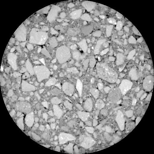
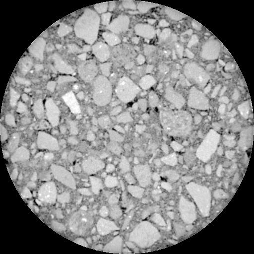
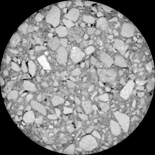
144 FIGURE 7.3 Reconstruction of 3D Specimen from Sectional Images 132

145 FIGURE 7.4 Reconstructed 3D Specimen before and after Testing 133

146 7.5 Methodology The following procedure is developed to evaluate the strain in the mixture Specimen Preparation The size of the specimen is approximately 300 x 125 x 75 mm. The beam specimen was prepared using the conventional rolling compaction. The aggregates are lime stone. Binder used was PG Image Acquisition Due to the energy limitation of the XCT system, the specimen cannot be directly scanned in its original size. The specimen was cut into three pieces and the cutting direction was perpendicular to the long axis of the original specimen as shown in Figure 7.5. Before and after testing, only the centerpiece was scanned. The size of centerpiece is 125 x 75 x 75mm. The image plane is consistent with the 75 x 75 mm cross-section. Before scanning, the centerpiece was marked to keep the specimen in the same position for the next scan after the testing. The specimen was scanned to obtain the first set of images. Then, the specimen was tested using the APA tester. After the testing, the centerpiece was scanned again. The two sets of images were then used to measure the particle displacements for micro and macro strains quantification. The image size is 512x512 pixels. One pixel represents 0.21 mm in the specimen. There are 200 sectional images for one specimen. The spacing between two images is 0.54mm. Scanning was in Y direction as shown in Figure 7.5 Due to the density differences of the mixture s constituents, the aggregates have the lightest color compared with mastics and air voids (Figure 7.6). Density 134

147 differences are the basis for the separation of the mixture phases. Cutting Edge Y Z X 125 FIGURE 7.5 Specimen Cutting Position for the APA test 135

148 Air Voids Aggregate Asphalt Binder FIGURE 7.6 Typical XCT Image APA Test During the testing, the three pieces were appropriately put together with the exact cutting face adjacent to each other in the APA. They were held in the position by the clamping system of the machine. During the test, the specimen was subjected a wheel load (100 lbs) by laying a linear tube along the centerline of its longitudinal edge. The cutting faces 136

149 were perpendicular to the direction of wheel traveling. The resulted rut depth is a function of load cycles, testing temperature, and is also the macro response of the specimen. Parallel to the load direction, the thickness of the specimen is larger than 3 inches, which is a representative size of an asphalt concrete specimen. Therefore, it is anticipated that the test results from the centerpiece can still represent the properties of the materials. The permanent deformations along the wheel path were measured as 6.38 mm after 8000 loading cycles Image Processing For this specific study, the objective of image processing is to separate aggregates from other phases and the boundaries of each aggregate. Imaging processing and analysis software, Image-Pro Plus, was used for processing these images. Each image was subjected to a threshold operation. Different threshold values were assigned to each image. In this study, aggregates were assigned to black in a binary image Image Analysis After the application of load, the aggregates had some rotation and translation within the mixture. In order to study the movement of the particles in the mixture, the particle should be represented in 3D. At first, each 2D particle in each image slice was identified between adjacent slices for reconstructing the 3D particle. In this study, a pattern recognition algorithm, based on the morphological characteristics of the particles, was applied to identify the particles in the images between adjacent slices as well as to identify the reconstructed 3D particles before and after testing. Once the particles are 137

150 tracked, the motions of the particles such as rotation and translation can be quantified and the strains can be further estimated. Since the particles are assumed as rigid bodies, their deformation is negligible under the application of wheel load. Therefore, permanent deformation of asphalt concrete mainly resulted from the rotation and translation of the particles, which was actually induced by the deformation of mastics around the particles. In the deformation process, particle parameters such as volume, surface area, and aspect ratio remain constants. The recognition of algorithm was based on the above assumption. To identify the matching particles in the specimen, a method presented by Wang (2004), which was used to study the granular material, was applied in the study. It involved two identification procedures. One is to identify particles between adjacent slices for reconstructing the 3D particles; the other one is to identify the reconstructed 3D particles before and after testing. For the first procedure, it is implemented through the following steps. The first step is to measure the sectional characteristics such as centroid coordinates X, Y, Z, area, and perimeter of the particle i on the j th slice. Image-Pro Plus software was used to obtain these geometric parameters of the particles. The second step is to find the matching particles between adjacent slices based on comparing the Similarity Index (SI), which was defined as: i i i SI (7.1) = xi, j xm, j+ 1 + yi, j ym, j+ 1 + Ai, j Am, j+ 1 + Pi, j Pm, j+ 1 Where x i j yi, j,, represent the coordinates of the mass center for particle i on j th slice; 138

151 A i, j represents particle cross-sectional area for particle i on the j th slice; i j P, represents particle cross section perimeter for particle i on the j th slice; m is the dummy index representing the top five nearest neighbors for the particle cross sections on (j+1) th slice. The nearest neighbors are defined by the distance between two cross sections shown as: D (7.2) 2 2 = ( xi, j xm, j+ 1) + ( yi, j ym, j+ 1) To find the nearest neighbors (denoted by dummy index m) in (j+1) th slice, distances from particle i in j th slice to all the particles in (j+1) th slice are compared. Only the top five nearest neighbor particles cross sections are used for SI matching. However, in some cases, the differences of the perimeters or areas of the particle cross-sections between two adjacent slices could be relatively large while the mass centers difference is small. The area and perimeter may actually increase noises for particle cross-section identification, and research indicated that mass center was the most important factor for particle detection (Wang, 2004). Therefore, Equation 7.1 was modified as: SI (7.3) = x i, j x m, j y i, j y m, j + 1 The section that has the minimum SI is considered as matching cross sections that belong to the same particle between two image slices. Practically, SI cannot be the only factor that controls the particle cross section identifications. There are some special cases that might confuse the detection. As it was shown in Figure 7.7, particle a in the j th slice disappeared in the (j+1) th slice; and particle b in the (j+1) th slice appears almost the same position as particle c in the j th slice. The above two conditions might also give a minimum 139

152 SI, but the cross-sections detected didn t belong to the same particle in the adjacent slices. Therefore, computer intelligence and human judgment were interactively used to implement the particle recognition decisions. In this study, a FORTRAN program was developed to automatically execute the above steps with the consideration of the above special cases. FIGURE 7.7 Special Cases for Particle Identification 140

153 The second procedure involves finding match particles before and after testing. Since the particles were treated as rigid bodies, the volumes of the particles would keep the same before and after testing. The identification procedure was based on the above assumption. The procedure to identify the particles before and after testing is briefly described as follows: The first step is to compare the mass center coordinates of the reconstructed 3D particles. For bonded material, the displacement inside the mixture is relatively small, which means the mass center of the particle before and after testing will not change much. Therefore, the similarity index (SI) based on the mass center coordinates was used as criterion to identify the particles. The second step is to compare the volumes of the particles before and after testing. The particles, which have the closest locations and volumes, belong to the same particle. The mass center ( X, Y, Z ) and volume (Vi) of particle i are calculated using the following equations: mc mc mc V i A A + 2 j 1 j H j 1 j (7.4) 141

154 X mc + ( A j 1 + A j ) H j 1 j ( x j 1 x j ) / 4 V i Y mc + ( Aj 1 + A j ) H j 1 j ( y j 1 y j ) / 4 V i (7.5) Z mc + ( A j 1 + Aj ) H j 1 j ( z j 1 z j ) / 4 V i Where x, y, z are the center coordinates of the cross-section of particle i on the j th slice; j j j A j is the cross sectional area of particle i on the j th slice; H j 1 j is the spacing between two adjacent slices ( H j 1 j = z j z j 1 ) Strain Computation: Macro Strain Once the particles before and after the testing were identified, the translation of the particles can be calculated from the mass center difference before and after testing, which was shown in the following equation: u = a X mc X b mc a v = Y mc Y b mc (7.6) 142

155 a w = Z mc Z b mc Where b represents before testing; a represents after testing. For each of four closest particles (i, j, k, l), the displacements in the x direction are defined as u, u, u, u, i j k l v, i, v j, vk vl in the y direction, and w i w j, wk, wl, in the z direction. For the simplest case, if a valid displacement field was linear interpolated in a tetrahedron, the displacement can be expressed as the following equation: u = a0 + a1x + a2 y + a3z v = b0 + b1 x + b2 y + b3 z (7.7) w = c0 + c1x + c2 y + c3z Where x, y and z are any coordinates in the tetrahedron before testing. a 0, a1, a2, a3, b 0, b1, b2, b3, and 0, c1, c2, c3 c are constants but vary from tetrahedron to tetrahedron. These constants can be obtained from the following matrix. 143

156 144 = l k j i l l l k k k j j j i i i u u u u a a a a z y x z y x z y x z y x ,, 1,,, 1,,, 1,,, 1, = l k j i l l l k k k j j j i i i v v v v b b b b z y x z y x z y x z y x ,, 1,,, 1,,, 1,,, 1, (7.8) = l k j i l l l k k k j j j i i i w w w w c c c c z y x z y x z y x z y x ,, 1,,, 1,,, 1,,, 1, The macro strain can be calculated as: a 1 x u x = = ε 2 b y v y = = ε 3 c z w z = = ε b 1 a y u x v xy + = + = ε (7.9) a 3 c x w z u xz + = + = ε b 3 c y w z v yz + = + = ε These strains were named as macro strain because they represent the average strain in the

157 tetrahedron. The algorithm of strain measurement was shown in Figure 7.8. Using the above equations, a FORTRAN code was developed to calculate the strain components in the tetrahedron. Results of x, y, z strains and shear strains on one plane are shown in Figure 7.9. Strains in these calculations follow the conventional manner: positive for tensile strain. Y direct strains, in the load direction, are larger than other direct strains. Meanwhile, strains in the area close to the load application zone are apparently larger than those in the zones farther from this zone. Strains in one tetrahedron were also shown in the following table. TABLE 7.1 Marco Strain for One Tetrahedron ε x ε y ε z ε xy ε xz ε yz

158 Center of Tetrahedron Y k l k l y b i i j y a i i j X x b i x a i Z b Before deformation a After deformation FIGURE 7.8 Algorithm of Macro Strain Measurement 146

159 X-Direct Strain Y-Direct Strain Z-Direct Strain XY Shear Strain XZ Shear Strain YZ Shear Strain FIGURE 7.9 Macro Strain Contours of the Specimen 147

160 Figure 7.10 shows the Y direction strain contour of the center section of the rutted area. In the figure, along the Y-axis the specimen from the top to the bottom, obtain the macro strain value ε z in every 10 mm. Then the total deformation in the Y direction can be calculated as Y = ε ydy = 6. 1 mm, which is close to result of macro deformation obtained from APA test, 6.38 mm. the difference might be caused by the image resolution or image processing. Figure 7.11 shows the Y direction strain contour of the edge section of the rutted area. Using the same deformation measurement method as for center-rutted area, the deformation for the edge-rutted area is 0.02 mm. the rutted profile, which obtained from experiment and measurement is compared in Figure FIGURE 7.10 Y-direction Strain of Center Rutted Area 148

161 FIGURE 7.11 Y-direction Strain Contour of Edge Rutted Area 149

162 Rut Depth (mm) Specimen Length (mm) Experimental Data Measured Data FIGURE 7.12 Comparison of Experimental and Measured Rutted Profile 150

163 7.5.7 Strain Computation: Permanent Strain in the Mastic Macro strains described in the previous step were the average strains that could be used to evaluate the overall properties of the mixture. However, it couldn t reflect the microbehavior of the mixture. As previously noted, aggregates in the mixture were treated as rigid bodies. The permanent deformation mainly resulted from the deformation in the mastics. Therefore, the strains in the mastics are important parameters to study the rutting mechanism in the mixture. It was calculated by considering the relative displacements between two particles A and B in Figure 7.13, which was obtained through the mass centers translations of two particles as shown in the following equation: u = u u ) cos α + ( v v ) cos β + ( w w ) cos γ (7.10) n ( A B A B A B Where u, u, v, v, w, w represent the mass center displacements of two particles A A B A B A B and B in the x, y and z directions. α, β, γ are the angles between the x, y and z axis and mass centers connection line. Assuming there is no discontinuity between the particles and the mastics, the normal strain in the mastic can be obtained by the following equation: u ε n n = (7.11) L Where L was expressed as the following equation: L = H r A r B (7.12) Where r A and r B are the radii of the two particles in the direction of the line connecting 151

164 their mass centers (Figure 7.14). Due to the difficulties in measuring the radii in a specific direction of irregular shapes in the 3D space, the particles were assumed as spheres that have the same volumes as the particles of irregular shapes in the above calculation. Therefore, their radii can be calculated from volumes. H is the distance between the mass centers of the two particles. It was defined by the following equation: H = ( xa xb ) + ( y A yb ) + ( z A zb ) (7.13) Y B B Y b A A Y a A A X X b A X a A Z b - before deformation a - after deformation FIGURE 7.13 Algorithm of Micro Strain Measurement 152

165 r B L r A Particle B Particle A Mass Center FIGURE 7.14 Radii of Two Irregular Particles 153

166 The micro strain for the same tetrahedron in the previous step is illustrated in the following table. TABLE 7.2 Strain in the Mastics Node X Y Z U V W Strain No. 1 (B) ε n = (B) ε n = (B) ε n = (B) ε n = (A) ε n = (A) ε n = (A) (A) (Notes: A represents after test; B represents before test) Comparing the results in Table 7.1 with those in Table 7.2, it can be found that the strain in the mastics was much larger. Tensile strain exists in the zone that is closed to the wheel load, which means it occurs in the compression zones. This result is 154

167 consistent with the properties of asphalt concrete. The dilation is due to the aggregate skeleton. In Figure 7.8, the configurations of the particles in one tetrahedron were compared before and after testing. The displacements were not very apparent. However, in Figure 7.15, when the particles were overlapped before and after testing, the displacement were evident in that P*-b represents the particles before the testing while P*-a represents the particles after the testing. FIGURE D Particle Configurations before and after Testing 155