What are we going to do?

Transcription

1 RBC Model Analyzes to what extent growth and business cycles can be generated within the same framework Uses stochastic neoclassical growth model (Brock-Mirman model) as a workhorse, which is augmented by a labor-leisure choice Business cycles reflect optimal response to stochastic movements in the evolution of technological progress. No role for monetary factors in explaining fluctuations ( real business cycles) 2 / 1

2 What are we going to do? We will document several empirical regularities ( stylized facts ) of business cycles We will use the standard neoclassical growth model as a tool to understand the causes of business cycles Using a model as a measurement tool requires 3 steps: Mapping the model s parameters to the data: Calibration Solving the model (we will use log-linearization) Comparing the model s outcome and the stylized facts 3 / 1

3 Real GDP in U.S. Want to understand aggregate economic activity: real GDP Figure: Krüger, Quantitative Macroeconomics: An Introduction 4 / 96

4 Use of Logarithms Assume variable Y grows at a constant rate g It follows that Y t = (1 + g) t Y 0 Taking (natural) logarithms log(y t ) = log[(1 + g) t Y 0 ] = log(y 0 ) + log[(1 + g) t ] = log(y 0 ) + t log[1 + g] If Y grows at a constant rate g, it will be a straight line with slope log[1 + g] g for small g 5 / 1

5 Use of Logarithms: Taylor Expansion The fact that log(1 + g) g is the result of a Taylor series expansion of log(1 + g) around g = 0: log(1 + g) = log(1) + g 0 1 = g 1 2 g g g 1 2 (g 0) (g 0) / 1

6 Isolating Cycles & Removing Trends Business cycles ˆ= deviations from long-run growth trend Let Y t be real GDP. Then log(y t ) = log(y trend ) + log(y cycle ) We are interested in the cyclical component: log(y cycle ) = log(y t ) log(y trend ) How to detrend the data? 7 / 1

7 Isolating Cycles & Removing Trends Different filters that perform this task Detrending First-difference filter Hodrick-Prescott (HP) filter And others (Bandpass,... ) They differ with respect to assumptions about the trend component 8 / 1

8 Removing Trends: Detrending Assume that trend is deterministic: Y t = (1 + g) t Y 0 e ut, u t (mean-zero, stationary) Taking log s (using log(1 + g) g) log(y t ) = log(y 0 ) + gt + u t The cyclical component log(y cycle ) is given by log(y cycle ) = u t = log(y t ) log(y 0 ) gt log(y 0 ) and g can be estimated by OLS Deterministic trend assumption has been challenged in the time-series literature (see e.g. Nelson/Plosser 1982) 9 / 1

9 Removing Trends: Differencing Assume that trend is stochastic: Y t = Y 0 e ɛt ɛ t = g + ɛ t 1 + u t, u t (mean-zero, stationary) Iterative substitution for ɛ t 1, ɛ t 2,... yields t 1 ɛ t = gt + u t j + ɛ 0 j=0 The cyclical component log(y cycle ) is given by log(y cycle ) = u t = log(y t ) log(y t 1 ) g This can be achieved by taking first differences & demeaning the sample average of log(y t ) log(y t 1 ). This implicitly assumes constant average growth rate g 10 / 1

10 Removing Trends: HP-Filter Solve the following minimization problem: +λ t=1 min log(yt trend ) T t=1 (log(y t ) log(y trend t )) 2 T [(log(yt+1 trend ) log(yt trend )) (log(yt trend ) log(yt 1 trend ))] 2 Results depend on λ. One can show that if λ = 0: log(y t ) = log(y trend t ) λ : log(y trend t ) = log(yt 1 trend) + g 11 / 1

11 HP-Filtered Real GDP Figure: λ = 1600,Krüger (2007). Quantitative Macroeconomics: An Introduction 12 / 96

12 Detrended GDP Figure: Solid: Det. Trend, Dots: Diff ed, Dashes: HP (DeJong/Dave (2007).Structural Macroe metrics) 13 / 96

13 Summary: Removing Trends & Isolating Cycles Cyclical component looks very different depending on our assumptions Choice of filter somewhat arbitrary To evaluate model: eliminate trends from the data generated by the model and actual data in the same way When working with quarterly data, be aware of seasonality. Adjust the data before filtering In the following: Look at HP-filtered data 14 / 1

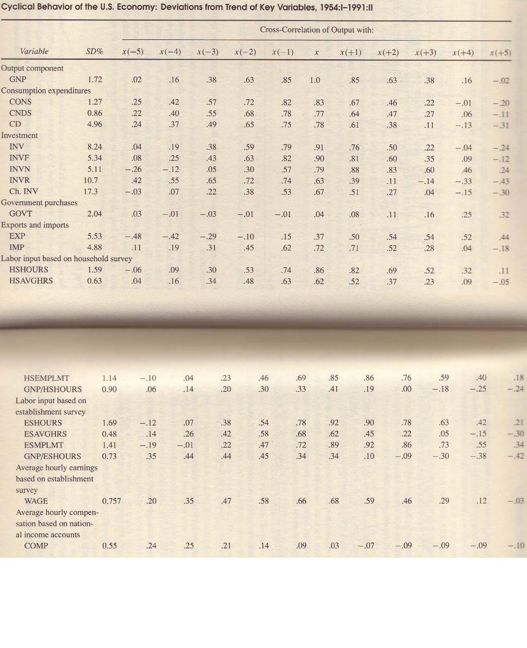
14 Stylized Facts We are interested in the amplitude of fluctuations the degree of comovement with real GNP whether there is a phase shift of a variable relative to the overall business cycle, as defined by cyclical real GNP 15 / 1

15 Stylized Facts Some labels: If the contemporaneous correlation coefficient of a variable with real GNP is positive (negative), we say it is procyclical (countercyclical) A variable leads the cycle if correlation coefficient of the series which is shifted forward w.r.t. real GNP is positive A variable lags the cycle if correlation coefficient of the series which is shifted backward w.r.t. real GNP is positive 16 / 1

16 Some observations: Stylized Facts Fluctuations in consumption and capital are smoother than output fluctuations Investment is much more volatile than output Total hours worked are almost as volatile as output The real wage and the real interest rate are quite smooth Consumption, investment and hours worked are very procyclical Productivity is also procyclical, but much less volatile than output Wages are uncorrelated with output 17 / 1

17 18 / 96

18 The Basic RBC Model: Introduction To what extent can stochastic neoclassical growth model account for these facts? We discipline the model by making it consistent with long-run growth 19 / 1

19 The Basic RBC Model: Introduction Model consists of Households Firms Other sectors (i.e. government) could be added Recall Brock-Mirman economy we discussed in Macro I 20 / 1

20 The Basic RBC Model: Introduction Households (HH) A large number of identical, infinitely lived HH HH maximize utility which they derive from consumption of goods and consumption of leisure (or disutility of work) HH supply labor to firms and rent out capital to firms HH use their income either for consumption or for buying investment goods which they add to their capital stock HH behave competitively taking all prices for given There is a representative household 21 / 1

21 The Basic RBC Model: Introduction Firms A large number of identical firms Firms rent capital and labor from households They produce a single good and take all prices as given Assume that they operate a constant returns to scale technology Perfect competition and constant returns to scale imply that the number of firms is indeterminate: representative firm 22 / 1

22 The Basic RBC Model Representative HH problem: [ ] max E 0 β t u(c t, 1 h t ) c t,h t such that t=0 k t+1 + c t = w t h t + (1 + r t )k t 0 c t 0 k t+1 k 0 given Recall that we could use sequence formulation to make uncertainty more explicit, as we did in Macro I. 23 / 1

23 The Basic RBC Model Remarks Rational expectations imply that household computes expectations using the correct probabilities Notice that there are only aggregate shocks (that affect the whole economy) but no idiosyncratic shocks (that affect the individual households differently) During the course we will also study the opposite case (no aggregate but idiosyncratic shocks) 24 / 1

24 The Basic RBC Model We can make use of the welfare theorems and study the planner s problem: such that max c t,h t E 0 [ ] β t u(c t, 1 h t )N t t=0 C t = c t N t K t+1 + C t = Z t F (K t, A t N t h t ) + (1 δ)k t A t+1 = (1 + g A )A t N t+1 = (1 + g N )N t Z t+1 = Zt ρ e ɛt, ρ (0, 1), ɛ t N(0, σ 2 ) 0 C t 0 K t+1 K 0, Z 0, N 0, A 0 given 25 / 1

25 The Basic RBC Model: Existence of Balanced Growth Path Balanced growth: growth in output, capital and consumption (per capita) grow over long periods of time Balanced growth is characteristic for most industrialized countries Long-run growth occurs at rates that are roughly constant over time (but may differ across countries) We need to impose certain restrictions on functional forms to guarantee existence of balanced growth path 26 / 1

26 The Basic RBC Model: Existence of Balanced Growth Path Where does economic growth come from? We think of increases in output at given levels of input through increase in technological knowledge which we take as exogenous Can be either labor-augmenting or capital augmenting 27 / 1

27 The Basic RBC Model: Existence of Balanced Growth Path Technology: Impose labor-augmenting technological progress A t and a production function that features constant returns to scale: Y t = Z t F (K t, A t N t h t ) where λy t = Z t F (λk t, λa t N t h t ) We will typically work with Cobb-Douglas technology Y t = Z t K α t (A t N t h t ) 1 α Here, technical progress can always be written as purely labor-augmenting 28 / 1

28 The Basic RBC Model: Existence of Balanced Growth Path Some notation: Define growth factor of variable V γ V V t+1 V t = 1 + g V Express variables in per-capita terms: y t Yt N t, k t Kt N t, c t Ct N t 29 / 1

29 The Basic RBC Model: Existence of Balanced Growth Path From resource constraint: γ k = k t+1 k t = y t c t + (1 δ)k t (1 + g N )k t On balanced growth path, γ k is constant This implies that yt k t and ct k t are constant as well Thus γ k = γ y = γ c on balanced growth path 30 / 1

30 The Basic RBC Model: Existence of Balanced Growth Path Verify existence on balanced growth path under the assumption about technology above: γ y = y t+1 F (1, X t+1 ) = γ k y t F (1, X t ) where X t Atht k t From this, we get γ y = γ k γ F and γ X = γ Aγ h γ k Therefore, γ k = γ y γ F = 1 γ X = 1 Hence, γ k = γ A γ h Notice that γ h = 1 (otherwise h 1 which is inconsistent with balanced growth) Therefore γ k = γ y = γ c = γ A on balanced growth path 31 / 1

31 The Basic RBC Model: Existence of Balanced Growth Path Return on labor supply: w A t F 2 ( k A, h) Along the balanced growth path, γ k = γ A Therefore, γ w = γ A How can it be that w is growing but labor supply is constant (γ h = 1)? Need to impose restrictions on preferences s.t. income and substitution effect of permanent increase in w cancel out 32 / 1

32 The Basic RBC Model: Existence of Balanced Growth Path Return on capital: r F 1 ( k A, h) which is constant along the balanced growth path Euler equation implies u 1 (c t, 1 h t ) = β(1 + r δ) u 1 (c t+1, 1 h t+1 ) where the RHS is constant along the balanced growth path Since γ c = γ A, consumption grows at a constant rate It follows that marginal utility of consumption has to change at a constant rate as well intertemporal elasticity of consumption independent of c 33 / 1

33 The Basic RBC Model: Implications of Balanced Growth Path The following utility function are consistent with a balanced growth path: 1. with θ, σ 0 2. and 3. or with θ, κ 0 with θ 0 u(c t, 1 h t ) = (c t(1 h t ) θ ) 1 σ 1 1 σ u(c t, 1 h t ) = log(c t ) θ (h t) 1+κ 1 + κ u(c t, 1 h t ) = log(c t ) + θlog(1 h t ) 34 / 1

34 The Basic RBC Model: Implications of Balanced Growth Path These specifications yield to the following optimality conditions for the intratemporal trade-off between consumption and leisure: θc t 1 h t = w t θh κ t c t = w t θc t 1 h t = w t 35 / 1

35 The Basic RBC Model: Implications of Balanced Growth Path Substitution effect: Increase in w t makes leisure more expensive Income effect: higher wages mean - for unchanged labor supply - higher income 36 / 1

36 The Basic RBC Model: Implications of Balanced Growth Path Consider the budget constraint in a static world (no intertemporal effects): c t = h t w t Plugging this into FOCs above, we find that effect of w t cancels out Income and substitution effects cancel out 37 / 1

37 The Basic RBC Model: Implications of Balanced Growth Path Recall that on balanced growth path, increase in w are permanent and r is constant Households budget constraint is the same as in the static case (see graph golden rule level of capital stock ) Income and substitution effects of wage changes cancel out No effect on labor supply Hence, γ w = γ A = γ c and γ h = 1 38 / 1

38 The Basic RBC Model: Implications of Balanced Growth Path Restriction on preferences has important implications for the ability of the model to generate fluctuations If capital is absent or if wages grow permanently, there is no endogenous response to exogenous productivity (King, Plosser and Rebelo 1988) Intertemporal substitution, stemming from temporary changes in productivity and transmitted through capital are key for generating amplification in the RBC model 39 / 1

39 The Basic RBC Model: Implications of Balanced Growth Path Given these restrictions, it is possible to define new variables that are constant in the long-run: k t = ỹ t = c t = K t (1 + g A ) t (1 + g N ) t = k t (1 + g A ) t Y t (1 + g A ) t (1 + g N ) t = y t (1 + g A ) t C t (1 + g A ) t (1 + g N ) t = c t (1 + g A ) t 40 / 1

40 The Basic RBC Model: Stationary Version such that max c t,h t E 0 [ t=0 ] β t ( c t(1 h t ) θ ) 1 σ 1 N t 1 σ (1 + g A )(1 + g N ) k t+1 + c t = Z t kα t ht 1 α + (1 δ) k t β t = β t (1 + g A ) t(1 σ) Z t+1 = Z ρ t e ɛt, ρ (0, 1), ɛ t N(0, σ 2 ) 41 / 1

41 The Basic RBC Model: First-Order Conditions Euler-Equation: [ ( 1+g A = βe ) ( ) t αz t+1 kα 1 h1 α t δ c σ ( ) ] t 1 θ(1 σ) ht+1 c t+1 1 h t (1) Intra-temporal labor-leisure trade-off: θ c t 1 h t = (1 α)z t kα t h α t (2) 42 / 1

42 Calibration: Introduction We want to know to what extent the model replicates business cycle facts Select parameter values such that model can be used as a measurement tool Select parameters such that deterministic version of model (no productivity shocks) is consistent with empirical facts about long-run growth 43 / 1

43 2 sets of parameter values Calibration: Strategy Direct empirical counterpart: estimated from the data No direct empirical counterpart: calibrated to match long-run averages in the data Some remarks: Distinction not always clear-cut Often disagreement about the correct parameter value Robustness checks to assess sensitivity of results should thus be good practice Alternative: estimate entire model (using for example Bayesian Maximum Likelihood) 44 / 1

44 Calibration: Long-Run Growth Rates Growth rates measure the change from one period to the next Need to decide about the length of a period in model Business Cycle analysis usually done on quarterly data Population growth g N : 1.1% per year. Per Quarter: g N = (1.011) Growth of GDP per capita g A : 2.2% per year. Per Quarter: g A = (1.022) / 1

45 Calibration: Curvature Utility Function Risk aversion is determined by σ: Higher values imply higher degree of risk aversion & stronger incentive for smooth consumption profile Standard estimates based on individual data: σ should be between σ = 1 & σ = 3 σ = 1 common in business cycle literature This implies u(c t, 1 h t ) = log(c t ) + θ log(1 h t ) 46 / 1

46 Calibration: Technology ỹ t = Z t kα t h 1 α t Long-run mean of Z t is Z 1 α is given by the capital share in total output s k rk Y = kα k α 1 h 1 α ỹ = α In the data, s k has (until recently) been constant over time and amounts to percent of total output Exact value depends on the treatment of income from self-employment, of housing and the government sector Here: α = / 1

47 Calibration: Depreciation Rate δ On balanced growth path: k t = k t+1 = k Budget constraint: (1 + g A )(1 + g N ) k t+1 = (1 δ) k t + (ỹ t c t ) }{{} (1 + g A )(1 + g N ) k = (1 δ) k + ĩ δ = ĩ k + 1 (1 + g A)(1 + g N ) ĩ k = on an annual level δ = ( )( ) / 1

48 Calibration: Discount Factor β On balanced growth path: c t = c t+1 = c With σ = 1, β = β The Euler-Equation simplifies to ( ) (1 + g) = β αỹ k + 1 δ k ỹ 3.32 on an annual level. The quarterly ratio is = Using α, δ, g we get β = / 1

49 Calibration: Weight of Leisure θ Rewrite condition?? (1 α)ỹ c = θ h 1 h h = 0.31: households spend 1 3 ỹ c = 1.33 This yields θ = 1.78 of their time working 50 / 1

50 Approximation Methods Model is very complex - in general it is not possible to derive explicit solutions Need to rely on approximation techniques We will learn two approaches: Make use of recursive structure and write down problem as a dynamic programm. Use value function iteration to approximate decision rules Directly work on the model s optimality conditions. Problem: non-linearity. Solution: (Log-)linear approximation of optimality conditions 51 / 1

51 Approximation Methods: Log-Linearization Here, we will log-linearize optimality conditions Approximate solution around steady-state Variables are expressed in % deviation from steady-state unit-free! 52 / 1

52 Log-Linearization Determine Constraints and FOCs Compute steady-state Log-linearize necessary conditions Solve for recursive equilibrium law of motion via the method of undetermined coefficients Analyze the solution via impulse-response analysis and simulation of second moments This follows the Uhlig (1997) procedure closely (also see homework). 53 / 1

53 Example Social Planner Problem: such that max C t E 0 [ t=0 ] β t C (1 σ) t 1 σ K t+1 + C t = Z t Kt α + (1 δ)k t Z t+1 = Zt ρ e ɛt, ρ (0, 1), ɛ t N(0, σ 2 ) 0 C t 0 K t+1 K 0 and Z 0 given 54 / 1

54 Example: Optimality Conditions + transversality condition C t + K t+1 = Z t Kt α + (1 δ)k t R t = αz t Kt α 1 + (1 δ) Ct σ [ = E t βc σ t+1 R ] t+1 Z t+1 = Zt ρ e ɛt, ρ (0, 1) 55 / 1

55 Example: Steady State Z = 1 C + K = K α + (1 δ) K C = Ȳ δ K ( R = α K α 1 + (1 δ) K = α R 1 + δ ) 1 1 α 1 = β R R = 1 β 56 / 1

56 Log-Linearization Each optimality condition can be re-written in terms of an implicit function: f ( x, ȳ) = 0 where x and ȳ are steady state values of x and y. By implicit differentiation or f ( x, ȳ) dx + x f ( x, ȳ) dy = 0 y f ( x, ȳ) x x f ( x, ȳ) + ȳ dx x dȳ y y = 0 (3) 57 / 1

57 Log-Linearization dȳ y = y ȳ ȳ ( log 1 + y ȳ ȳ ) = log ȳ y ŷ ŷ: % deviation from steady-state Re-write (??): [ ] [ ] f ( x, ȳ) f ( x, ȳ) ˆx x + ŷ ȳ 0 (4) x y Linear in ˆx and ŷ Alternatively, take log s first and then perform first-order Taylor expansion around log( x) and log(ȳ) 58 / 1

58 Log-Linearization: Let s Do It! Budget Constraint: K t+1 + C t Z t K α t (1 δ)k t = 0 This is a function in 4 variables: K t+1, C t, Z t and K t Applying (??) gives K ˆk t+1 + Cĉ t Z K α (ẑ t + αˆk t ) (1 δ) K ˆk t 0 59 / 1

59 Log-Linearization: Let s Do It! Euler-Equation: [ βe t C σ t+1 R ] t+1 C σ t = 0 Contains 3 variables: C t+1, R t+1 and C t Applying (??) and using 1 = β R yields βe t [ σ C ( σ 1) Cĉ t+1 R + C σ R ˆr t+1 ] + σ C ( σ 1) Cĉ t 0 E t [ σĉ t+1 + ˆr t+1 ] + σĉ t 0 E t [σ(ĉ t ĉ t+1 ) + ˆr t+1 ] 0 60 / 1

60 Log-Linearization: Let s Do It! Return-Function: 3 variables: R t, Z t and K t Applying (??) yields R t αz t K α 1 t (1 δ) = 0 R ˆr α Z K α 1 (ẑ t + (α 1)ˆk t ) 0 61 / 1

61 Collecting Equations K ˆk t+1 + Cĉ t Z K α (ẑ t + αˆk t ) (1 δ) K ˆk t = 0 E t [σ(ĉ t ĉ t+1 ) + ˆr t+1 ] = 0 R ˆr α Z K α 1 (ẑ t + (α 1)ˆk t ) = 0 ẑ t+1 = ρẑ t + ɛ t 62 / 1

62 Log-Linearization Write down optimality conditions: (resource) constraints and FOCs Compute steady-state Log-linearize optimality conditions Solve for recursive equilibrium law of motion via the method of undetermined coefficients Analyze the solution via impulse-response analysis and simulation of second moments 63 / 1

63 Method of Undetermined Coefficients We want to find policy functions: recursive law of motion We have to solve system of linear differential equations, which is given by the log-linearized equilibrium conditions Use Method of Undetermined Coefficients 64 / 1

64 Method of Undetermined Coefficients We postulate a linear recursive law of motion ˆk t+1 = ν kk ˆk t + ν kz ẑ t ˆr t = ν rk ˆk t + ν rz ẑ t ĉ t = ν ck ˆk t + ν cz ẑ t Solve for the undetermined coefficients ν kk, ν kz, ν rk, ν rz, ν ck, ν cz Similar approach to Guess and Verify 65 / 1

65 Method of Undetermined Coefficients Let s see how it works. The necessary condition for the interest rate is given by which we can re-write to by making use of R ˆr α Z K α 1 (ẑ t + (α 1)ˆk t ) = 0 ˆr (1 β(1 δ))(ẑ t (1 α)ˆk t ) = 0 (5) 1 β = R = α Z K α 1 + (1 δ) (??) depends on parameter values only 66 / 1

66 Method of Undetermined Coefficients We can now determine the coefficients of the policy function for r t : ˆr = (1 β(1 δ))(ẑ t (1 α)ˆk t ) ν rk ˆkt + ν rz ẑ t = (1 β(1 δ))(ẑ t (1 α)ˆk t ) ν rk ˆkt + ν rz ẑ t = (1 β(1 δ))ẑ t (1 β(1 δ))(1 α)ˆk t thus ν rk = (1 β(1 δ))(1 α) ν rz = (1 β(1 δ)) 67 / 1

67 Method of Undetermined Coefficients Proceed in similar manner for the other equations After a while, you ll end up with a quadratic equation in ν kk : 0 = ν 2 kk γν kk + 1 β (6) where γ = (1 β(1 δ))(1 α)(1 β + βδ(1 α)) σαβ β 68 / 1

68 Method of Undetermined Coefficients Equation (??) has two solutions We are looking for ν kk < 1: stable root If ν kk > 1, k keeps growing (falling) which will violate transversality condition (the non-negativity constraint) Use stable root to calculate ν kz, ν rk, ν rz, ν ck, ν cz 69 / 1

69 Log-Linearization Determine Constraints and FOCs Compute steady-state Log-linearize necessary conditions Solve for recursive equilibrium law of motion via the method of undetermined coefficients Analyze the solution via impulse-response analysis and simulation of second moments 70 / 1

70 Log-Linear Approximation: Appraisal Works almost always has become standard procedure in the literature Computationally very fast, but linearization tedious Local method as optimal policies are computed near steady-state: works only for small deviations Implicitly assumes certainty equivalence 71 / 1

71 Log-Linear Approximation: Certainty Equivalence Log-linear version of Euler-Equation: E t [σ(ĉ t ĉ t+1 ) + ˆr t+1 ] 0 σĉ t E t [σĉ t+1 + ˆr t+1 ] Compare this to the deterministic Euler equation: σĉ t σĉ t+1 + ˆr t+1 72 / 1

72 Log-Linear Approximation: Certainty Equivalence The property that the decision rule depends only on the first moment of the distribution that characterize uncertainty is called certainty equivalence Higher moments (e.g. variance) do not matter for the choices This is a problem if true solution depends on higher moments (e.g. if there is precautionary saving) 73 / 1

73 Alternative Methods Alternative local solution methods: Optimal Linear Regulator Excellent alternative for social planner problems, avoids tedious linearization Second-order approximation (Schmitt-Grohé/Uribe 2004) Does not impose certainty equivalence Global solution methods such as successive approximation of the value/policy function Compute optimal choice for all feasible values of the state variables Precise but slow 74 / 1

74 Recursive Law of Motion After this long detour, we return to our model with endogenous labor Using the calibrated parameters, we can compute the policy functions with the help of the procedure outlined before ˆk t = 0.97ˆk t ẑ t ĉ t = 0.63ˆk t ẑ t ĥ t = 0.27ˆk t ẑ t 75 / 1

75 Recursive Law of Motion We can make use of this to trace out the response of our economy to technology shocks: Impulse responses We can shock the economy repeatedly and trace out the responses: Simulation Useful for understanding the qualitative and quantitative properties 76 / 1

76 Technology Shocks Production Function where y t = Z t k α t (1 + g) t h 1 α t Z t+1 = Z ρ t e ɛt, ρ (0, 1), ɛ t N(0, σ 2 ) We want to estimate ρ and σ 2 77 / 1

77 Technology Shocks Taking logs log(y t ) = log(z t ) + αlog(k t ) + (1 α)log(h t ) + (1 α)tlog(1 + g A ) log(z t ) = log(y t ) (αlog(k t ) + (1 α)log(h t ) + (1 α)tlog(1 + g A ) Z t is the Solow-Residual Estimate ρ and σ from log(z t ) = ρlog(z t 1 ) + ɛ t In the data, techn. shocks are quite persistent: ˆρ = / 1

78 Impulse Responses In t = 0, set all variables to 0 In t = 1, technology shock ɛ 1 > 0 In t = 2,..., T, ɛ t = 0. Trace out ˆk t and ẑ t using their recursive law of motion Given ˆk t and ẑ t for t = 2,..., T, trace out all other variables 79 / 1

79 Simulation Given ˆσ, simulate sequence of {ɛ t } T t=0 number generator using a random Pick some initial k 0 and z 0 Calculate recursively ẑ t+1 = ˆρẑ t + ɛ t ˆk t+1 = ν kk ˆkt + ν kz ẑ t With that, obtain all other variables 80 / 1

80 RBC Mechanism How does the economy react to a temporary increase in productivity? Response of labor supply is particularly important: change in h t determines whether the model amplifies or dampens the fluctuations generates by ẑ t 81 / 1

81 RBC Mechanism The FOC s of the representative household in our case are: θc t 1 h t = w t (7) where w t (1 α)z t kt α ht α and Euler-Equation: [ ( )] ct 1 = βe t R t+1 c t+1 (8) 82 / 1

82 RBC Mechanism We can combine (??) and (??) to get [ ] w t 1 h t 1 = βe t R t+1 w t+1 1 h t+1 If there were no uncertainty, this equation could be written β = 1 w t+1 R t+1 w }{{ t } W t 1 h t+1 1 h t (9) where W t is the wage growth in present value terms 83 / 1

83 RBC Mechanism Recall that on a balanced growth path, w t grows at a constant rate, hence w t+1 w t is constant Moreover, R t+1 = R on a balanced growth path Hence, W = W Therefore 1 h t+1 1 h t must be constant By construction, this has to hold for all utility functions consistent with balanced growth path! 84 / 1

84 RBC Mechanism In general, labor supply depends on the relative wage. If w 1 is higher than w 2 (because of a temporary productivity shock), households supply more labor today than tomorrow the interest rate. A higher interest rate induces households to increase their labor supply today as returns are higher The sensitivity of these effects depends on the intertemporal elasticity of substitution (which is 1 in this example) 85 / 1

85 RBC Mechanism The IES of leisure is given by d 1 h t+1 1 h t dw t W t = 1 h t+1 1 h t ( ) dln 1 ht+1 1 h t dln (W t ) = 1 The IES of labor supply is then given by approximately 1 h h... obtain this by a sequence of approximations of the type ln (x + 1) x when x 0 Estimates using micro data suggest that the Frisch elasticity of labor supply is around 0.5. Aggregate data suggests a higher Frisch elasticity (since aggregate data incorporate the extensive margin of labor supply) 86 / 1

86 Baseline 7 Impulse responses to a shock in technology investment 6 Percent deviation from steady state output technology labor interest capital consumption Years after shock 87 / 96

87 Low Peristence (ρ =.8) 8 investment Impulse responses to a shock in technology 7 6 Percent deviation from steady state output labor technology 0 interest capital consumption Years after shock 88 / 96

88 Baseline 20 Simulated data (HP-filtered) Percent deviation from steady state consumption interest labor technology output capital investment Year 89 / 96

89 Baseline Std. Dev output capital cons labor interest investment techno / 96

90 RBC Assessment Kydland and Prescott (1982), Nobel Prize Laureates (2004): A competitive equilibrium model was developed and used to explain the autocovariances of real output and the covariances of cyclical real output with other aggregate economic time series...results indicate a surprisingly good fit in light of the model s simplicity. 91 / 1

91 RBC: Assessment Output fluctuates quite a bit, but less than in the data Consumption, investment and labor input are very procyclical, as in the data Investment is much more volatile, as in the data Factor prices are quite smooth, as in the data However, labor input is less volatile than output Correlation of all variables with output is very high, too high compared to the data Productivity is nearly as volatile as output (low internal propagation of model) 92 / 1

92 RBC: Reasons for Model s Weakness Technology shock is very persistent, therefore wages adjust smoothly, generating little fluctuations in labor As a result, too little fluctuations in labor input and weak internal propagation Critique: the assumed Frisch elasticity of labor supply is much larger than estimates based on micro data The high correlation of all variables with output is due to the fact that there is only one shock 93 / 1

93 Extensions: Labor Markets Generating realistic fluctuations in aggregate labor supply without imposing an IES on the individual level is a big challenge See problem set for a solution that was proposed by Hansen (1985) Moreover, there is no notion of unemployment in the frictionless RBC model Modeling unemployment can be an important mechanism to generate amplification and persistence (see Hall (1998: Labor Market Frictions and Employment Fluctuations) 94 / 1

94 Extensions: TFP Shocks Are they correctly measured? What is their interpretation? (Are deep recessions really periods of technical regress?) Are technical shocks really exogenous with respect to policy? See King and Rebelo (1999): Resuscitating Real Business Cycles and Rebelo (2005): Real Business Cycle Models: Past, Present, and Future 95 / 1

95 Extensions: Asset Prices and Financial Intermediation Counterfactual behavior of asset prices More recently: How to incorporate monetary and financial frictions? Kiyotaki and Moore (2009): Liquidity, Business Cycles, and Monetary Policy and Gertler and Kiyotaki (2009): Financial Intermediation and Credit Policy in Business Cycle Analysis Workhorse model of monetary frictions: the New Keynesian model 96 / 1

96 Micro versus macro elasticities Micro/labor economists often argue that Frisch elasticity is low Macro economists view the (aggregate) Frisch elasticity to be large Key insight: if there exists an extensive margin of labor supply, then the aggregate elasticity will generally be much higher than the micro elasticities 97 / 1

97 Frisch elasticity with intensive margin Let the utility function be given by u (c, h) = v (c) h1+1/φ φ Consider first the Frisch elasticity if labor supply is chosen at the intensive margin, given a wage w 98 / 1

98 Intensive margin Frisch elasticity (cont.) Intra-temporal first-order condition: MU h = w MU c When MU c is held constant (so as to evaluate the Frisch elasticity), the solution is h 1 φ = w MU c log h = φ log w + φ log (MU c ), so the Frisch elasticity is φ 99 / 1

99 Extensive margin (Rogerson, 1988) Suppose now that labor supply is indivisible: h {0, h} Problem: how deal with discrete choice? Solution: assume complete markets and convexify indivisibility using lotteries 100 / 1

100 Convexification using lotteries Assume there exists a lottery which determine if a worker is employed or not If employed, the allocation is h = h c = c e If unemployed, the allocation is h = 0 c = c u Note: due to complete markets and no externalities, we can use the welfare theorems and instead formulate problem as a planner problem 101 / 1

101 Convexification using lotteries (cont.) Planner problem is to choose a probability ξ of employment. Objective function for planner becomes { [ ] h 1+1/φ max ξ v (c e ) 1 + 1/φ subject to ξw h + a = ξc e + (1 ξ) c u First-order conditions w.r.t. c u and c e are ξv (c e ) λξ = 0 (1 ξ) v (c u ) λ (1 ξ) = 0, which implies c e = c u + (1 ξ) [v (c u ) 0] } 102 / 1

102 Convexification using lotteries (cont.) Rewrite the planner problem imposing c e = c u = c, { [ ] max ξ h 1+1/φ v (c) 1 + 1/φ = max {v (c) ξ B} where B = h 1+1/φ / (1 + 1/φ) is a constant + (1 ξ) [v (c) 0] Note that the Frisch elasticity of aggregate labor supply is infinity! The is an example where there is aggregation, although the representative (mongrel) agent has preferences which are fundamentally different from the preferences of the individual households } 103 / 1