Gaussian Mixture Filters in Hybrid Positioning

Transcription

1

2 Tampereen teknillinen yliopisto. Julkaisu 813 Tampere University of Technology. Publication 813 Simo Ali-Löytty Gaussian Mixture Filters in Hybrid Positioning Thesis for the degree of Doctor of Technology to be presented with due permission for public examination and criticism in Tietotalo Building, Auditorium TB109, at Tampere University of Technology, on the 7th of August 2009, at 12 noon. Tampereen teknillinen yliopisto - Tampere University of Technology Tampere 2009

3 ISBN (printed) ISBN (PDF) ISSN

4 Abstract Bayesian filtering is a framework for the computation of an optimal state estimate fusing different types of measurements, both current and past. Positioning, especially in urban and indoor environments, is one example of an application where the powerful mathematical framework is needed to compute as a good position estimate as possible from all kinds of measurements and information. In this work, we consider the Gaussian mixture filter, which is an approximation of the Bayesian filter. Especially, we consider filtering with just a few components, which can be computed in real-time on a mobile device. We have developed and compared different Gaussian mixture filters in different scenarios. One filter uses static solutions, which are possibly ambiguous, another extends the Unscented transformation to the Gaussian mixture framework, and some filters are based on partitioning the state space. It is also possible to use restrictive, inequality constraints, efficiently in Gaussian mixture filters. We show that a new filter called the Efficient Gaussian mixture filter outperforms other known filters, such as Kalman-type filters or particle filter, in a positioning application. We also show that another new filter, the Box Gaussian mixture filter, converges weakly to the correct posterior. All in all we see that the Gaussian mixture is a competitive framework for real-time filtering implementations, especially in positioning applications.

5

6 Preface The work presented in this thesis was carried out in the Department of Mathematics at Tampere University of Technology during the years I want to express my sincere gratitude to my supervisor Prof Robert Piché for his skilful guidance and encouragement during my doctoral studies. I am grateful to my colleagues in the Personal Positioning Algorithms Research group and in the department, especially Dr Niilo Sirola, Dr Kari Heine, Tommi Perälä and Henri Pesonen, for enlightening discussions and constructive feedback. I would like to thank Dr Jari Syrjärinne from Nokia Corporation for different perspectives and encouraging comments, the preexaminers Dr Simon Julier and Dr Oleg Stepanov for their comments and suggestions. The financial support of Tampere Graduate School in Information Science and Engineering, Nokia Corporation and Nokia Foundation are gratefully acknowledged. I am very grateful to my family, especially my dear wife Anna for hers love and support all these years and my wonderful son Onni. I would like to dedicate this thesis in memory of my sons Joonatan and Oiva. To God be the glory for all the things He has done in my life. Tampere, May 2009, Simo Ali-Löytty iii

7

8 Contents List of publications Related publications vi viii Nomenclature ix Abbreviations ix Symbols x 1 Introduction 1 1 Background Problem statement Literature review Kalman filter Kalman-type filters Nonlinear filters Development of the Gaussian mixture filter Restrictive information Approximate the likelihood as GM Approximate the prior as GM Approximate the posterior as GM Convergence result of BGMF Hybrid positioning results Sensitivity analysis of GMFs Summary of hybrid positioning results Some notes for real world implementation Conclusions and future work References 39 Publications 49 v

9 List of publications This thesis consists of an introduction and the following publications, in chronological order: P1. Consistency of three Kalman filter extensions in hybrid navigation (with Niilo Sirola and Robert Piché). European Journal of Navigation, 4(1), P2. A modified Kalman filter for hybrid positioning (with Niilo Sirola) In Proceedings of the 19th International Technical Meeting of the Satellite Division of the Institute of Navigation (ION GNSS 2006), Fort Worth TX, September P3. Gaussian mixture filter in hybrid navigation (with Niilo Sirola) In Proceedings of the European Navigation Conference 2007 (ENC 2007), Geneva, May P4. Gaussian mixture filter and hybrid positioning (with Niilo Sirola) In Proceedings of the 20th International Technical Meeting of the Satellite Division of the Institute of Navigation (ION GNSS 2007), Fort Worth TX, September P5. Efficient Gaussian mixture filter for hybrid positioning In Proceedings of the IEEE/ION Position, Location and Navigation Symposium (PLANS 2008), Monterey CA, May P6. On the convergence of the Gaussian mixture filter Research report 89, Tampere University of Technology, Institute of Mathematics, The author s role in the shared publications: P1: The author developed the general inconsistency test, wrote the filters code, ran the tests and wrote the manuscript. P2: The author developed a method for using restrictive information with Kalman-type filters, wrote the code as well as the manuscript. P3: The author developed the algorithms and part of the code, and wrote the manuscript. P4: The author developed the algorithms and part of the code, and wrote the manuscript. vi

10 The main contributions of the publications are: P1: The general inconsistency test without any assumptions of the shape of the distribution. The publication also shows that nonlinearity is not significant in satellite measurement, but it might be significant in base station range measurement. P2: A method for taking into account restrictive information (inequality constraints) in Kalman-type filters. This method is also applied to hybrid positioning using base station sector and maximum range information (cell-id) with Kalman-type filters. P3: A method for applying static solutions (in our case likelihood peaks) in the filtering framework, that is approximate likelihood as Gaussian mixture. Publication also presents how we can use static solutions to robustify Kalman-type filters. P4: Sigma Point Gaussian Mixture Approximation (SPGMA), which extends sigma-points to the Gaussian mixture filter framework. The publication also presents how to measure nonlinearity, when EKF possibly fails. P5: Box and Efficient Gaussian Mixture Filters (BGMF and EGMF), that split the state space into sets using parallel planes. BGMF and EGMF give better performance in hybrid positioning simulations than the particle filter. P6: The convergence results of BGMF. BGMF increases number of components only to the dimensions where it is necessary and BGMF allows the reduction of the number of components. vii

11 Related publications The following publications relate to the subject, but are either redundant or contain only minor contribution from the author: R1. Simo Ali-Löytty, Niilo Sirola, and Robert Piché. Consistency of three Kalman filter extensions in hybrid navigation. In Proceedings of the European Navigation Conference GNSS 2005 (ENC 2005), Munich, July R2. Niilo Sirola and Simo Ali-Löytty. Local positioning with parallelepiped moving grid. In Proceedings of the 3rd Workshop on Positioning, Navigation and Communications (WPNC 06), March 16, R3. Niilo Sirola and Simo Ali-Löytty. Moving grid filter in hybrid local positioning. In Proceedings of the European Navigation Conference (ENC 2006), Manchester, May 7-10, R4. Niilo Sirola, Simo Ali-Löytty, and Robert Piché. Benchmarking nonlinear filters. In Nonlinear Statistical Signal Processing Workshop (NSSPW 2006), Cambridge, September R5. Matti Raitoharju, Niilo Sirola, Simo Ali-Löytty, and Robert Piché. PNaFF: a modular software platform for testing hybrid positioning estimation algorithms. In Proceedings of the 5th Workshop on Positioning, Navigation and Communication (WPNC 08), Hannover, March 28, R6. Tommi Perälä and Simo Ali-Löytty. Kalman-type positioning filters with floor plan information. In Third International Workshop on Broadband and Wireless Computing, Communication and Applications (BWCCA 2008), Linz, November 24-26, R7. Ville Honkavirta, Tommi Perälä, Simo Ali-Löytty, and Robert Piché. A comparative survey of WLAN location fingerprinting methods. In Proceedings of the 6th Workshop on Positioning, Navigation and Communication (WPNC 09), Hannover, March 19, R8. Simo Ali-Löytty. On the convergence of box mixture filters. In IEEE Transactions on Automatic Control (submitted). viii

12 Nomenclature Abbreviations B BGMA BGMF BLUE cdf CPU EGMF EKF EKF2 GM GMF GML GPS ID IEKF KF LKF PF PNaFF RMS SPGMA SPGMF UKF UT WLAN 2D 3D 6D Byte Box Gaussian Mixture Approximation Box Gaussian Mixture Filter Best Linear Unbiased Estimator cumulative density function Central Processing Unit Efficient Gaussian Mixture Filter Extended Kalman Filter Second Order Extended Kalman Filter Gaussian Mixture Gaussian Mixture Filter Gaussian Mixture Likelihood Global Positioning System Identity Iterated Extended Kalman Filter Kalman Filter Linearized Kalman Filter Particle Filter Personal Navigation Filter Framework Root Mean Squares Sigma Point Gaussian Mixture Approximation Sigma Point Gaussian Mixture Filter Unscented Kalman Filter Unscented Transformation Wireless Local Area Network two dimensional three dimensional six dimensional ix

13 Symbols infinity k lower index k represents time t k α i weight of i th GM component Ȧ novel polyhedron approximation of restrictive area A Square root of symmetric positive semidefinite matrix A, such as A= A A T A<B x T (B A)x> 0 for all x 0 c g parameter of conventional GM approximation d i j distance between mixture components[p3, Page 834] e i vector whose i th component is one and others are zero E(x) expectation value of random variable x Err app error, sup ξ F x (ξ) F x app (ξ) F state transition matrix F x cumulative density function (cdf) of random variable x h measurement function H linear measurement function or Jacobian of h Ḧ ki Hessian of i th component of function h k I identity matrix K Kalman gain l parameter of BGMA[P5] n eff approximation of effective sample size n gm number of GM components n pf number of particles n thr threshold value n x dimension of variable x natural numbers,{0,1,2,3,...} N parameter of BGMA[P6] N n (ˆx,P) Gaussian distribution with parametersˆx n and symmetric positive semidefinite matrix P n n x

14 Nˆx (x) density function of non-singular N P n(ˆx,p) p c (x) continuous density function p gm (x) density function of GM p x (x),p(x) density function of random variable x p(x k x k 1 ) transitional density p(x k y 1:k 1 ) prior (density function) p(x k y 1:k ) posterior (density function) p(y k x k ) likelihood P covariance of posterior P covariance of prior P x y E (x E(x)) y E y T P(A) probability of event A Φ cdf of N 1 (0,1) Q covariance of state model noise real numbers R covariance of measurement noise τ parameter of SPGMA tr(a) trace of matrix A n n, tr(a)= n A i=1 i,i U(a,b] uniform distribution with support(a,b] u prior bs unit vector from prior mean to base station v measurement noise V(x) covariance of random variable x ω i weight of i th sigma point w state model noise w (i) weight of i th particle of PF x prior state ˆx estimate of x, usual mean of x x 2 A weighted squared norm x 2 A = x T Ax χ sigma-point x usually state of the system x (i) i th particle x (i) g i th grid point on conventional GM approximation x y conditional probability distribution of x when condition y is fixed y usually measurement y 1:k set of measurements y 1,...,y k xi

15

16 CHAPTER 1 Introduction This thesis consists of an introduction and six published articles. The purpose of this introductory chapter is to give a short unified background of the problem and summarise the results of publications[p1 P6]. 1 Background Personal positioning has become very popular in recent years. In good signal environments, such as open-sky environments, a satellite based positioning system, e.g. Global Positioning System (GPS, which is also a popular abbreviation for any positioning device), provides accurate and reliable positioning. However, in poor signal environments, such as urban canyons or indoors, satellite based positioning systems do not work satisfactorily or at all. One possible solution for this problem is to also use other possible measurements and information in positioning. There are plenty of possible measurements sources, e.g. local wireless networks such as cellular networks[26, 53, 79, P1] or WLAN[3, 46, 65, R7] and map or floor plan information[18, 20, 40, R6],[51, 76, 83]. We call 1

17 positioning that uses measurements from many different sources hybrid positioning. Many of these possible measurements are so called signals of opportunity, which are not originally intended for positioning, furthermore many of these measurements are highly nonlinear. For these reasons, conventional positioning algorithms such as the extended Kalman filter [P1] or the minimum least squares estimator[r4] do not work satisfactorily in hybrid positioning. More sophisticated measurement fusion methods for hybrid positioning are needed. One possible fusion method is the Bayesian method, which is a probabilistic method[43, 64]. The Bayesian method enable different kinds of measurement and information to be fused. Futhermore, under some conditions it is possible to compute an optimal estimator recursively, which is an important property for real-time implementation. Unfortunately, it is not possible to compute this Bayesian solution analytically. Therefore, plenty of different approximate solutions, called filters, exist for this problem. For the rest of this thesis, we study these filters. 2 Problem statement The problem of estimating the state of a stochastic system from noisy measurement data is considered. We consider the discretetime system with a nonlinear measurement model: Initial state: x 0 (1a) State model: x k = F k 1 x k 1 + w k 1 (1b) Measurement model: y k = h k (x k )+v k (1c) where k \{0}, vectors x k 1 n x and y k n y k represent the state of the system and the measurement, respectively. Matrix F k 1 n x n x is the known state transition matrix, and w k 1 n x is the state model noise with known statistics. Function h k : n x n yk is a known measurement function, and vk n y k is the measurement noise with known statistics. Subscript k represents time t k. The aim of Bayesian filtering is to find the conditional 2

18 probability distribution given all current and past measurements, called the posterior and denoted x k y 1:k, where y 1:k={y1,...,y k }. We consider the Bayesian filtering problem because the knowledge of the posterior enables one to compute an optimal state estimate with respect to any criterion. For example, the minimum mean-square error estimate is the conditional mean of x k [8, 63]. We assume that noises w k and v k are white, mutually independent and independent of the initial state x 0 ; these assumptions allow posteriors to be computed recursively. We use the abbreviation V(w k )=Q k and V(v k )=R k for the covariance of the state model noise and the covariance of the measurement noise, respectively. We assume that initial state x 0 has density function p x 0= px0 y 1:0. If noises w k 1 and v k have density functions p wk 1 and p vk, respectively, then the posterior can be determined according to the following relations[17, 63]. Prediction: p(x k y 1:k 1 )= p(x k x k 1 )p(x k 1 y 1:k 1 )dx k 1 (2a) Update: p(x k y 1:k )= p(y k x k )p(x k y 1:k 1 ) p(yk x k )p(x k y 1:k 1 )dx k (2b) where the transitional density (also referred to as transition equation) p(x k x k 1 ) = p wk 1 (x k F k 1 x k 1 ) and the likelihood p(y k x k )=p vk (y k h k (x k )). We call the distribution x k y 1:k 1 the prior. Usually assumptions that noises w k 1 and v k have density functions are too strict. In some cases, the state model noise or the measurement noise does not have density function; this happens when we know that some components of the state are constant in time or our measurements contain restrictive information[p2], respectively. Throughout the remainder of this work, it is assumed that: Initial state x 0 has density function. Either state noise w k 1 has density function p wk 1, or state transition matrix F k 1 is nonsingular. Measurement noise v k has stricly positive density p vk or v k = 0 and y k =h k (x k ) p(x k y 1:k 1 )dx k > 0. 3

19 These assumptions guarantee that the posterior has a density function p(x k y 1:k ). Because the state transition function is linear, then the prior (prediction step), or at least the mean and covariance of the prior, is usually easy to compute. For example, results for Gaussian mixture case are given in[p6, Theorem 6]. So the biggest challenge in solving this Bayesian filtering problem is how to update the prior to obtain the posterior (update step). An illustration of our problem is in Figure 1, which presents the posterior when the prior 1 is Gaussian and we have two measurements, one linear 2 and one range 3 measurement, with (zero mean independent) Gaussian noise. Figure 1: Posterior density with Gaussian prior, one linear measurement, one range measurement, and Gaussian noise. We see that a crucial question in developing filters is how to store the distribution for the next time step. As we will see in Section 3 this is also one criterion for classifying filters. Note that the illustration in Figure 1, as well as other illustrations in Figures 2-9, are in 2D for practical reasons. 4 The real positioning applications are usually in 6D or higher dimensional state space. However, these illustrations, Figures 1-9, give a quite good idea of our problem and solutions. 1 x N , = 1 1 x+ v linear, v linear N 1 0, = x I + v range, v range N 1 0, These illustrations are computed using MATLAB-software and grid points. 4

20 The goal of this work is to develop an efficient filter with respect to computational and memory requirements. However, more important property than efficiency is that the filter is consistent[p1, R1],[50] and informative. Roughly speaking, a filter is consistent if the true estimation error is smaller than the estimated error, and informative if the difference of these errors is small. 3 Literature review In this section, we give a brief literature review of filtering. We consider the problem that is presented in Section 2 and the filters that we have used in publications[p1 P6]. For further information see e.g.[5, 8, 13, 22, 29, 56, 57, 63, 71, 80]. This section contains different interpretations of the celebrated and well known Kalman Filter (KF)[39] (Section 3.1), Kalman-type filters (Section 3.2) and nonlinear filters (Section 3.3) especially Gaussian mixture filter, which we study also in Section Kalman filter If the measurement function h k (1c) is linear and all the noises and the initial state are Gaussian, then posterior x k y 1:k is Gaussian, and its mean and covariance can be computed exactly using KF[2, 27]. KF considers the system: Initial state: x 0, V(x 0 )=P 0 (3a) State model: x k = F k 1 x k 1 + w k 1, V(w k 1 )=Q k 1 (3b) Meas. model: y k = H k x k + v k, V(v k )=R k (3c) where initial estimate (mean of initial state) isˆx 0, covariance P 0 is non-singular, noises w k 1 and v k have zero mean and covariances R k are non-singular. KF algorithm is given as Algorithm 1. However, this Bayesian interpretation is not the only interpretation of KF. We present other interpretations of KF: the Best Linear Unbiased Estimator (BLUE) interpretation and a deterministic interpretation. 5

21 Algorithm 1: Kalman filter 1. Start with initial estimateˆx 0 and estimate error covariance P 0. Set k= Prior estimate of state at t k isˆx k = F k 1ˆx k 1, and estimate error covariance is P k = F k 1 P k 1 FT k 1 + Q k Posterior estimate of state at t k isˆx k =ˆx k + K k yk H kˆx k, and estimate error covariance is P k =(I K k H k )P k, where Kalman gain K k = P k HT k Hk P k HT k + R 1. k 4. Increment k and repeat from 2. BLUE interpretation of Kalman filter BLUE interpretation drops the assumptions that initial state and noises are Gaussian and seeks unbiased and linear estimator 5 which minimizes the cost function E( x k ˆx k 2 ). It can be shown that the posterior estimate of KF at t k (Algorithm 1) minimizes that cost function, see for example[2, 5, 10, 39]. Deterministic interpretation of Kalman filter Consider the deterministic least-squares problem ˆx k = argmin x k ˆx 0 x 0 2 P k n=1 w n 1 2 Q 1 n 1 + v n 2 R 1 n, where w n 1 = x n F n 1 x n 1 and v n = y n H n x n. Here we assume that all necessary matrices are non-singular. Nowˆx k is the same as the posterior estimate of KF at t k (Algorithm 1) see example[38]. Note that this interpretation is truly deterministic: there are no assumptions of noise statistics or independence. 5 Estimatorˆx k is unbiased if E(x k ˆx k )=0and linear ifˆx k = A ˆxk 1 matrix A is arbitrary. 6 y k, where

22 We conclude that KF is a good choice for the linear system even if we do not know the noise statistic exactly or what the interpretation of the problem is. Unfortunately, in the general, nonlinear measurement function case, these three problems usually produce different solutions. Therefore, in the nonlinear case, it is more important to think about the interpretation of the measurement and the state than in the linear case. In this thesis, as mentioned, we have chosen the Bayesian interpretation of the state and our goal is to compute the posterior, see Section 2. For an example of the frequentist interpretation see[91]. 3.2 Kalman-type filters Because KF works well for linear systems (3) there are many KF extensions to the nonlinear system (1). We call these extensions Kalman-type filters. Kalman-type filters approximate only the mean (estimate) and covariance (error estimate) of the posterior. If necessary, a Kalman-type filter approximates the posterior as Gaussian with those parameters. Many Kalman-type filters are based on BLUE. Let x ˆx x E = and V = y ŷ y Px x P y x P x y P y y (4) then the BLUE of the state x is[8] ˆx=ˆx + P x y P 1 y y y ŷ E (x ˆx)(x ˆx) T = P x x P x y P 1 y y P y x. (5) Kalman-type filters use BLUE recursively, so that at every time instant the Kalman-type filter approximates these expectations (4) based on previous state and error estimates and computes new state and error estimates using (5), e.g. Algorithms 2-4. Naturally, different Kalman-type filters do these approximations using different methods. Next, we present some of these approximations. Maybe the best know KF extension is the Extended Kalman Filter (EKF)[5, 8, 22, 29, 57, 63, 71]. EKF is based on BLUE and it linearizes 7

23 Algorithm 2: Extended Kalman filter 1. Start with the meanˆx 0 = E(x 0 ) and the covariance P 0 = V(x 0 ) of the initial state. Set k = Prior mean of state at t k isˆx k = F k 1ˆx k 1, and prior covariance is P k = F k 1P k 1 F T k 1 + Q k Posterior mean of state at t k isˆx k =ˆx k +P x y k P 1 y y k yk ŷ k and posterior covariance is P k = P k P x y k P 1 y y k P T x y k, where P x y k = P k HT k, H k= h k (ˆx k ), P y y k = H k P k HT k + R k and ŷ k = h k (ˆx k ). 4. Increment k and repeat from 2. the measurement function h k (1c) around the prior mean and uses this linearization to compute the necessary expectations (4)[2, 8]. EKF algorithm for system (1) is given as Algorithm 2. This EKF Algorithm 2 is used in publications[p1 P5, R1 R6]. It is also possible to compute higher order EKF, which takes into account the higher order terms of the Taylor series of the measurement function. For example, Second Order Extended Kalman Filter (EKF2) takes into account the second order terms of the Taylor series[8]. EKF2 algorithm for system (1) is given as Algorithm 3. This EKF2 Algorithm 3 is used in publications[p1 P3, R1, R4 R6]. EKF2 uses the assumption that the posterior is Gaussian, contrary to EKF, which does not use this, usually incorrect, assumption. Modified Gaussian Second Order Filter[29, 57] is the same as EKF2. One big drawback of EKF and the higher order EKF is that the approximation of the measurement function is computed in the prior mean estimate, so if it is incorrect then the approximation of the measurement function is incorrect and the next estimate of the prior mean is incorrect, and so on. One example of a situation where EKF estimate veers away from the true route and gets stuck in an incorrect solution branch is given in[p1]. One approach to avoiding this kind of situation is to use different linearization points that do 8

24 Algorithm 3: Second order extended Kalman filter 1. Start with the meanˆx 0 = E(x 0 ) and the covariance P 0 = V(x 0 ) of the initial state. Set k = Prior mean of state at t k isˆx k = F k 1ˆx k 1, and prior covariance is P k = F k 1P k 1 F T k 1 + Q k Posterior mean of state at t k isˆx k =ˆx k +P x y k P 1 y y k yk ŷ k and posterior covariance is P k = P k P x y k P 1 y y k P T x y k, where P x y k = P k HT k, H k= h k (ˆx k ), ŷ k = h k (ˆx )+ 1 n yk e k i tr Ḧ 2 ki P k, i=1 n yk n yk P y y k = H k P k HT+ R + 1 e k k 2 i e T j i=1 Ḧki = h k i (ˆx k ) and tr Ḧki P k Ḧk j P. k 4. Increment k and repeat from 2. not depend on the prior, if possible. The name of that kind of KF extension is Linearized Kalman Filter (LKF)[22, 71]. One possible choice for the linearization point is likelihood peak(s), see[p3] or the mean of a truncated Gaussian, see[p5]. Of course, if we have more than one linearization point, we usually end up to Gaussian mixture filter, see Section 3.3. Another possibility is to generate linearization points using the state model; this idea is used in[47, 48]. It is also possible to compute EKF (or LKF), use the posterior mean estimate as a linearization point of LKF and iterate this procedure. The name of that kind of filter is Iterated Extended Kalman Filter (IEKF)[8, 29]. Note that IEKF computes the maximum a posterior estimate not the posterior mean estimate[8]. One drawback of EKF and the higher order EKF is that we have to compute the derivative of the measurement function analytically, which is not always possible or practical. Because of this, there are many derivative-free Kalman filter extensions. Note that in some cases, computing derivative analytically is not a problem at 9

25 all[r1]. Central difference filter[68], first-order divided difference filter[60] and Unscented Kalman Filter (UKF)[33, 35, 36, 37] are examples of derivative-free Kalman-type filters. These filters are also referred to as linear regression Kalman filters[49] and sigmapoint Kalman filters[88]. These filters use different numerical integration methods to compute the expectations (4). For example, UKF uses so called Unscented Transformation (UT)[35] that approximates expectation values of x N n (ˆx,P) E(h(x))= h(ξ)p x (ξ)dξ 2n i=0 ω i h(χ i ), (6) whereω i andχ i are so called extended symmetric sigma-point set of distribution N n (ˆx,P), which are given in Table 1.1[36]. Table 1.1: Extended symmetric sigma-point set of N n (ˆx,P) Index (i ) Weight (ω i ) sigma-point (χ i ) 0 ω 0 ˆx 1 ω 1,...,n 0 ˆx+ n Pe 2n 1 ω i 0 1 ω n+ 1,...,2n 0 ˆx n Pe 2n 1 ω i n 0 Approximation (6) is accurate if function h is third order polynomial[33]. In Table 1.1, the weight of the mean pointω 0 < 1 is a freely selectable constant. The choiceω 0 = 1 n is justified because 3 it guarantees that approximation (6) is accurate for some fourth order polynomial[36]. However, if we use negative weightω 0, it is possible to produce non-positive semidefinite posterior covariance P k and usually this causes problems. Ifω 0 = 2 and n = 1 3 then UT coincides with three points Gauss-Hermite rule, which has also been applied to Kalman-type filter framework; Gauss-Hermite filter[28]. UT needs 2n + 1 points and three point Gauss-Hermite rule generalization to higher dimension needs 3 n points, and thus UT and Gauss-Hermite rules coincide only in the one dimensional case[28, 36]. 10

26 UKF algorithm for system (1) is given as Algorithm 4. This UKF Algorithm 4 is used in publications[p3, P4, P5, R4, R6]. The extended symmetric sigma point set used in Algorithm 4 is the conventional choice of sigma points[33, 37], but there are also other possible choices[36] such as the simplex sigma-point set, which use the minimum number of sigma-points (n +1)[31]. It is also possible to scale sigma-points so that the predicted covariance is certainly positive semidefinite[30]. Algorithm 4 assumes that the state model noise w is Gaussian and exploits the linearity of the state model (1b), so it is not precisely the same as the conventional UKF. Publication [P4] extends UKF to Gaussian mixture filter framework, where every sigma point is replaced by a Gaussian distribution. Algorithm 4: Unscented Kalman filter 1. Start with the meanˆx 0 = E(x 0 ) and the covariance P 0 = V(x 0 ) of the initial state. Set k = Prior mean of state at t k isˆx k = F k 1ˆx k 1, and prior covariance is P k = F k 1P k 1 F T k 1 + Q k Posterior mean of state at t k isˆx k =ˆx k +P x y k P 1 y y k yk ŷ k and posterior covariance is P k = P k P x y k P 1 y y k P T x y k, where P x y k = 2n i=0 P y y k = R k + ω i χi ˆx k h k (χ i ) ŷ k T, ŷk = 2n i=0 2n i=0 ω i h k (χ i ) ŷ k h k (χ i ) ŷ k T. ω i h k (χ i ) and Hereω i andχ i are extended symmetric sigma-point set of distribution N n ˆx k k,p given in Table Increment k and repeat from 2. This list of different interpretations, variations and extension of Kalman-type filters is not exhaustive. For example, it is possible to use UKF to maintain and propagate information about the higher order moments[32, 34, 87]. 11

27 3.3 Nonlinear filters If the true posterior has multiple peaks as in Figure 1, it is unlikely that a Kalman-type filter that computes only the mean and covariance achieves good performance. Hence, we have to use more sophisticated nonlinear filters. A sophisticated nonlinear filter is one that has convergence results. Possible filters are e.g. grid mass filters[45, 75, 76, R2, R3], point mass filters[9, 11, 63, 70], particle filters[6, 16, 17, 21, 24, 25, 63] and Gaussian mixture filters[4, 5, 78, 82, P3 P6]. In this section, we consider particle filters and Gaussian mixture filters. Particle filter A particle filter (PF) or the sequential Monte Carlo, or Bayesian bootstrap filter simulates a sample (particles with weights) from the posterior distribution and approximates the posterior and especially the moments of the posterior using these weighted particles. A particle filter algorithm for system (1) is given as Algorithm 5. Algorithm 5: Particle filter Here we denote particles with superscript i= 1,...,n pf : x (i) k the i th particle at time t k. 1. Initialise samples from the initial distribution x (i) and assign all weights to w (i) 0 = 1 2. Simulate particles x (i) k and compute weights of particles w (i) k being 0 p x 0 (x),. Set k= 1. n pf from proposal distribution p(x k x (i) = w(i) k 1 p(y k x (i) k ). k 1 ) 3. Normalize weights and compute posterior mean and covariance using particles. 4. Resample (Algorithm 6) if effective sample size is smaller than some threshold value. 5. increment k and continue from 2. Note that Algorithm 5 is only one special case for system (1), actually quite a narrow case, of particle filters. This particle filter Algorithm 5 is used in publications[p2 P6, R2 R6]. It is well know 12

28 that without the resampling step (Step 4 in Algorithm 5) the degeneracy phenomenon occur, which means that after a certain number of recursive steps, all but one particle will have negligible normalized weights[63]. We use systematic resampling[41] (Algorithm 6) every time when the effective sample size (approximation)[42] n eff = n pf i=1 1 (i) w k is smaller than some threshold value n thr. 2 Algorithm 6: Systematic resampling Here we denote the current particles by x (i) and their weights by w (i). This algorithm simulates n pf particles x (i) with equal weights w (i) = 1 from discrete distribution defined by current particles and n pf weights Simulate the starting point: z 1 U 0, and set i= 1. n pf 2. Compute current comparison point z i = z 1 +(i 1) 1 n pf 3. Set w (i) = 1 and x (i) = x (j), where j is set in such a way that n pf j 1 k=1 w(k) < z i j k=1 w(k) 4. Stop, if i= n pf, otherwise increment i and continue from 2. The particle filter has several convergence results (see e.g.[16, 17, 25]), especially weak convergence results when there are a finite number of measurements and all measurement are fixed. The definition of weak convergence is found for example in[p6, Definition 8]. Even though the particle filter is very flexible, it requires that the likelihood function p(y k x k ) is strictly positive, because otherwise it is possible that all the weights are zero which destroys the particle filter. Unfortunately, all likelihoods of our system (1) are not strictly positive. One heuristic method of handling the situations where all weights are zero is to re-initilize particle filters using, e.g. EKF, which is what we are using in our publications, but after that the convergence results do not hold anymore. It is also possible to use (a bank of) UKF or another Kalman-type filter to compute the proposal distribution (Step 2 in Algorithm 5) 13

29 of PF[89, 90]. Note that if we change the proposal distribution, the equation of weight will also change (Step 2 in Algorithm 5). Gaussian mixture filter Gaussian Mixture Filter (GMF), also called Gaussian sum filter, is a filter whose approximate prior and posterior densities are Gaussian Mixtures (GMs), a convex combination of Gaussian densities. We assume (see Section 2) that the prior and the posterior distributions have density functions, but in general GM does not necessarily have a density function[p6, Definition 4]. GMF is an extension of Kalmantype filters. One motivation to use GMF is that any density function p x may be approximated as density function of GM p gm as closely as we wish in the Lissack-Fu distance sense[14, Chapter 18] 6,[52, 78]: p x (x) p gm (x) dx. (7) The outline of the conventional GMF algorithm for system (1) is given as Algorithm 7 (for detailed algorithm, see e.g.[p5, P6]). Here we assume that the initial state x 0, the state model noise w k 1 and the measurement noise v k are GMs. Because the initial state and the posterior approximations are GMs then also the prior approximations at each step are GMs (Step 2), see[p6, Theorem 6]. Algorithm 7: Gaussian mixture filter 1. Start with initial state x 0. Set k= Compute prior approximation x k. 3. Approximate x k as a new Gaussian mixture if necessary. 4. Compute GM posterior approximation x k. 5. Reduce the number of components. 6. Increment k and repeat from 2. 6 Note that for allε>0there is a continuous density function p c (x) with compact support such that p x (x) p c (x) dx<ε[66, Theorem 3.14]. 14

30 The heart of the GMF is the approximation of an arbitrary density function with a Gaussian mixture (Step 3). There are numerous approaches to do that. We present one conventional method. More methods are in Section 4. The density function of GM approximation p gm of a density function p x is defined as[4] n gm p gm (x) i=1 p x (x (i) g (i) )Nx g c g I (x), (8) where the mean values x (i) g are used to establish a grid in the region of the state space that contains the significant part of the probability mass, n gm is the number of grid points and c g > 0 is determined so that the error in the approximation, e.g. Lissack-Fu distance (7), is minimized. It can be shown that p gm (x) converges almost everywhere uniformly to any density function of practical concern as the number of components n gm increase and c g approaches zero[4, 78]. Moreover, Lissack-Fu distance (7) converges to zero. This Step (Step 3) is executed only when it is necessary. One possible criterion is to check if all prior covariances do not satisfy inequality P i <εi, for some predefinedε, where P i is the covariance of the i th component[5]. A more sophisticated method is to execute Step 3 if nonlinearity is significant[p4]. The update step of Algorithm 7 (Step 4) is usually computed as a bank of EKFs, see detailed algorithm e.g.[p6, Algorithm 2]. It is possible to compute the update step using a bank of another Kalman-type filters[p3] or bank of PFs[44]. There are also other methods of computing the posterior weights than what is in the algorithm given in[p6, Algorithm 2], e.g. methods based on quadratic programming[28]. Furthermore, in some cases, it is possible to combine Step 3 and Step 4, e.g. in EGMF[P5]. The crucial point when applying GMF to real-time implementations is the number of components GMF uses. The number of components easily explodes if we do not use some method to reduce the number of components (Step 5). The possible methods are, e.g. forgetting[78, P3, P6], merging[67, 78, P3, P6], resampling[p3], clustering[67] or minimizing some cost function, see e.g. Step 3 or[55]. One possible method for this problem is taking 15

31 a sample from the posterior and using the weighted expectationmaximization algorithm to fit an m -component GM [89], but usually this method is quite slow. It can be shown that GMF (Algorithm 7) with some assumptions and specific approximations convergences (weakly) to the correct posterior when the number of components increases[5], [P6, Section IV]. Even if we use component reduction, especially in higher dimension, conventional approximations (8) yield GMF which is not applicable in real-time implementation. However it may be possible to derive GMF that works notably better than Kalman-type filters and uses only a few components, see Section 4 and publications[p3 P6]. 4 Development of the Gaussian mixture filter In this section, we summarize the contributions of publications[p2 P6] to the development of GMF. We use the assumptions of Section 2 except that we assume that initial state x 0, state model noise w k 1 and measurement noise v k are GMs. Moreover, we use Gaussian mixture posterior approximation. 4.1 Restrictive information Restrictive information tells that the state is inside some area A. Restrictive information can be modelled with inequality constraints[69, 72, 73]. There are many different methods of taking into account inequality constraints e.g.[23, 62, 69, 72, 73]. However, in our view, the most natural way is to model the restrictive information as a measurement (1c) with zero noise which produces likelihood which is one inside A and zero outside A [P2] 7. An example of using restriction information in such a way is in Figure 2, where on the left hand side is posterior without using restrictive information and the right hand side using it. 7 This approach also independently proposed in [72] and [73], which were published after abstract of[p2] was submitted. 16

32 Figure 2: Left: the same as Figure 1. Right: the same posterior with 120 base station sector information. The left hand side of Figure 2 is the same as Figure 1, where prior is Gaussian and we have two measurements, one linear and one range measurement with Gaussian noise. Restrictive information that is used on the right hand side of Figure 2 is 120 base station sector information. Note that the vertical scales of the left and right plots are different. In this case, we see that sometimes restrictive information notably improves state estimation. Because of this, it is important that we can use that kind of information with Kalmantype filters. This is the focus of publication[p2]. If the area A is restricted by two parallel planes and the distribution of the state is Gaussian (or GM), it is possible to efficiently compute the mean and covariance of the restricted state[69, 72, P2]. In publication[p2], we develop an approximation to extend this method to cases where the area A is a polyhedron and apply it to base station cell-id information[79] (see[p2] and Figure 3). The left hand side of Figure 3 is the same as the right hand side of Figure 2, which presents the optimal way to use 120 base station sector information. The right hand side of Figure 3 uses the method presented in publication[p2] to approximate base station sector information and after that it uses conventional EKF. When we compare the left and right hand sides of Figure 3, we see that this approximate way to use base station sector information is quite good. One advantage of this new approximation method (box- 17

33 Figure 3: Left: the same as the right hand side of Figure 2. Right: posterior approximation using first approximated 120 base station sector information (see[p2]) and then EKF. method) is that it approximates restrictive area as polyhedron Ȧ[P2, Figure 1] so that the mean and covariance of the restricted posterior can be computed using standard one dimensional Gaussian cumulative density function and basic algebra. We use cell-id information as restrictive information also in publications[p4, P5]. It is also possible to construct restrictive information from a digital map or floor plan[r6]. The method of using restrictive information with Kalman-type filter[p2] is a basis and an inspiration of the Box Gaussian mixture approximation of Section 4.3 and publications[p5, P6]. 4.2 Approximate the likelihood as GM In Section 4.1 we allowed the components of the measurement noise to be zero, which means that the measurement noise does not have density function. However, henceforth we assume that the measurement noise is GM with density function p vk. Based on our assumptions, the prior (approximation) is always GM. So it is convenient to consider only Gaussian prior case with Gaussian measurement noise p vk (v)=n 0 R k (v). The generalizations to the GM 18

34 cases are straightforward, see[p3, P6]. Our problem is to approximate/compute the posterior (2b) where the likelihood is and the prior is p(x k y 1:k ) p(y k x k )p(x k y 1:k 1 ), p(y k x k )=N 0 R k yk h k (x k ) p(x k y 1:k 1 )=N x k(x P k ). k As we mentioned in Section 3.3, the usual method of computing the posterior is to linearize the measurement equation around the prior mean (EKF)[P3]: h k (x k ) h k (x k )+h k (x k )(x k x k ). Quite often, when there are enough measurements, this is a good approximation, but when the likelihood has several peaks in the neighbourhood of the prior mean, this approximation fails. One possible way to avoid this problem is to approximate the likelihood as GM[P3] n gm p(y k x k ) N 0 yk R k h k (z j ) h (z k j)(x k z j ), (9) where z j, j= 1,...,n gm are the likelihood peaks 8 (also referred to as static solutions). An example for using this approximation is shown in Figure 4. The left hand side of Figure 4, which is the same as Figure 1, is the posterior when the prior is Gaussian and we have two measurements, one linear and one range measurement with Gaussian noise. z 8 If h k (x) depends only on the first d elements of x n peak and z=, where z rest z peak d, maximizes the likelihood function then z is acceptable likelihood peak if and only if z rest = 0. Furthermore, it is reasonable to consider only clearly distinct likelihood peaks. 19

35 Figure 4: Left: the same as Figure 1. Right: posterior approximation using GM likelihood approximation, Err GML = (10). The right hand side of Figure 4 is the posterior approximation using a two-component likelihood GM approximation (9). The error Err app = sup F x (ξ) F x app (ξ), (10) ξ where F x (ξ)=p(x ξ) is cdf of the correct posterior and F x app (ξ) is cdf of the approximated posterior. Motivation for using that error statistic come from definition of weak convergence[p6, Definition 8]. Usually this error statistic has to be computed using some multidimensional numerical integration method and so it is not very useful for extensive testing of different filters[76, Section 5]. The error of Figure 4 posterior approximation is Err GML = This error is rather small if we compare it with the error of EKF approximation Err EKF = We show that in the hybrid positioning case, using this approximation when likelihood has several peaks outperforms Kalman-type filters such as EKF, EKF2 and UKF (see[p3]). In the hybrid positioning case, it is sometimes possible to compute the likelihood peaks in closed form[7, 74, 77], publication[p3, Appendix B] also presents some new cases where it is possible. Moreover, the method of approximating likelihoods as GM, is one way to apply multiple static position solutions in a filtering framework. Approximating likelihood as GM has also been applied in the radar tracking applications[85, 86]; publication[86] approximates the 20

36 measurement noise v k (1c) as GM and then converts these mixture components to the state space. It is a nice idea, but it does not work with range measurements, because small measurement noise in the range measurement does not generate small likelihood components. It is possible to approximate almost all likelihoods inside a interesting region with sufficient accuracy as GM (see Algorithm 7 Step 3). For example in Figure 5 the likelihood of 2D range measurement with Gaussian noise is approximated as GM with 18 components using the conventional method (8). 9 However, this method usually needs a huge amount of GM components, especially in higher dimension. Furthermore, many of these components are unnecessary because after multiplying the likelihood and the prior, usually, many of these components have almost zero weight. Hence, it is not worthwhile to apply this approximation method to real-time implementations. Figure 5: Left: exact likelihood of 2D range measurement with Gaussian noise. Right: GM 18 components approximation of likelihood using (8). Publication[P3] also presents a non-bayesian approach to robustifying GMF using likelihood peaks: if the measurements are unlikely, we add new component(s) to the posterior with appropriate weights. 9 That kind of approximation is used as initial state GM approximation in rangeonly target tracking application[19]. 21

37 These new components approximate the likelihood function so that the means of the components are likelihood peaks. This method is justified if there is a possibility that our prior is wrong. This method is related to Hough transformation[59] that uses the sum of likelihood functions instead of a product as in Bayesian filtering. 4.3 Approximate the prior as GM In Section 4.2, we computed the posterior (2b) p(x k y 1:k ) p(y k x k )p(x k y 1:k 1 ), by approximating likelihood p(y k x k ) as GM. In this section, we use a bank of EKFs to compute the posterior approximation, but before the update step we approximate the prior p(x k y 1:k 1 ) as GM. It can be shown that if GM approximation of the prior converges to the correct prior, and the covariance of GM approximation becomes smaller, the posterior approximation of the bank of EKFs converges to the correct posterior[5, P6]. More discussion about the convergence results is in Section 4.5. However, the main interest is not in a convergence result but in developing a filter that works well also with a few mixture components. In this section, we consider two ways to approximate the prior as GM with a small number of mixture components: the Sigma Point GM approximation[p4] and the Box GM approximation[p5, P6]. Another possibility to approximate prior as GM is to approximate the state model noise w k 1 (1b) as GM with small covariance[4]. So if the posterior GM components have small covariances, this approximation guarantees that the next prior components have small covariances too. Sigma Point GM approximation The Sigma Point GM approximation (SPGMA) is an extension of sigma-point to GM framework. SPGMA is given in Table 1.2[P4, P5]. In Table 1.2, we use a slightly different parametrization than in publication[p4]. Parameter τ [0, 1] defines the size of the covariances of SPGMA. Special cases areτ=0when SPGMA is actually the 22

38 same as the original Gaussian andτ=1when SPGMA is the same as the extended symmetric sigma-point set of distribution N n (ˆx,P), Table 1.1. Parameterα 0 is the weight of the GM component whose mean is the same as the mean of the original distributionˆx. Table 1.2: Sigma Point GM approximation of distribution N n (ˆx,P) Index (i ) Weight (α i ) Mean (ˆx i ) Covariance (P i ) 0 α 0 ˆx (1 τ 2 )P 1 α 1,...,n 0 ˆx+τ n Pe 2n 1 α i (1 τ 2 )P 0 1 α n+ 1,...,2n 0 ˆx τ n Pe 2n 1 α i n (1 τ 2 )P 0 Publication[P4] shows that SPGMA has the same mean, covariance and third moments as the original distribution N n (ˆx,P)[P4, Appendix B]. An example of using this approximation is presented in Figure 6. Figure 6: Left: the same as Figure 1. Right: posterior approximation using SPGM prior approximation, Err SPGMF = (10). The left hand side of Figure 6, which is the same as Figure 1. The right hand side of Figure 6 is the posterior approximation using the SPGM prior approximation, with parametersα 0 = 0.5 and τ=0.6. This approximation is also called the Sigma Point Gaussian Mixture Filter (SPGMF)[P5]. The error (10) of this approximation is 23

39 Err SPGMF = This error is better than the error of EKF approximation but worse than the error of GM likelihood approximation of Section 4.2. Note that SPGMA does not need the knowledge of likelihood peaks so it can be used in a wider range of situations than the GM likelihood approximation. In publications[p4] and[p5] we show that SPGMA with the bank of EKFs (SPGMF[P5]) gives almost the same results as the particle filter in the hybrid positioning case. Box GM approximation The idea of the Box GM approximation (BGMA) is to partition the state space into sets A i, where i = 1,...,n gm, and approximate the distribution inside every set with one GM component using moment matching, see Table 1.3. Table 1.3: BGMA of n-dimensional distribution, whose density function is p x (ξ). Sets A i, where i= 1,...,n gm, are the partition of n. Weight (α i ) Mean (ˆx i ) Covariance (P i ) p A x (ξ)dξ x p x(ξ) dξ T px (ξ) x ˆxi x ˆxi dξ i A i α i A i α i The moment matching method guarantees that the mean and covariance of BGMA coincide with the original distribution[p6, Theorem 18]. Here we assume that the distribution is non-singular Gaussian but this basic idea is also applicable to other distributions that have a density function. The partition of the state space can be constructed, for example, using parallel planes[p5, Figure 1] or using a (bounded) polyhedron[p6, Figure 1]. One major advantage of BGMA is that we can use current measurements in an intelligent way to construct the partition of the state space. For example, with range measurement[p5] it is reasonable to align the parallel planes such that the normal vector is perpendicular to the vector u prior bs 24

40 from the prior mean to the base station because this minimizes the effect of nonlinearity[p4, Equation (8)]. Vector u prior bs is the eigenvector of the Hessian matrix of the range measurement whose eigenvalue is 0[R1]. An example for using BGMF[P5] is presented in Figure 7. The left hand side of Figure 7 is the same as Figure 1. The right hand side of Figure 7 is the posterior approximation using BGMA of the prior[p5], with parameter l= =Φ Black lines in the Figure 7 illustrate parallel planes 10 which are using for partitioning the state space. The error (10) of this BGMF approximation is Err BGMF = We see that BGMF with three components gives better approximation than SPGMF with five components. So our illustrative example supports the conclusion of publication[p5] that BGMF outperforms SPGMF. Figure 7: Left: the same as Figure 1. Right: posterior approximation using BGMA of prior, Err BGMF = (10). Black lines illustrate parallel planes that are using for partitioning the state space These planes (lines) satisfy equation a T (x ˆx)=±1.04[P5, Section IV-B], where a= n n, n= , P= T Pn andˆx = (see page 4). Note 40 a T Pa= 1 and a T u prior bs = 0 where (see page 24) u prior bs = 0 ˆx. 25

41 4.4 Approximate the posterior as GM In Section 4.2 we computed the posterior (2b) p(x k y 1:k ) p(y k x k )p(x k y 1:k 1 ), by approximating the likelihood p(y k x k ) as GM, and in Section 4.3 we approximated the prior p(x k y 1:k 1 ) as GM. In this section, we directly approximate the posterior as GM. This method is called Efficient Gaussian Mixture Filter (EGMF)[P5] and it is related to BGMF when the partition (sets A i, i= 1,...,n gm ) of the state space is constructed using parallel planes, see Section 4.3. The idea of EGMF is to approximate the posterior inside every set A i with one GM component. The i th GM component is computed using LKF, where the linearization point is the same as the i th linearization point of BGMF x p x(ξ) dξ Table 1.3. The final posterior component is A i α i the moment matching approximation of the truncated (using set A i ) output of LKF (see more details in publication[p5]). 11 Figure 8: Left: the same as Figure 1. Right: posterior approximation using EGMF, Err EGMF = (10). An example of using EGMF[P5] is presented in Figure 8. The left hand side of Figure 8 is the same as Figure 1. The right hand side 11 If the state is constant, that is the state model (1b) is x k = x k 1, then it is possible to use the truncated Gaussian as a prior without approximating it as a Gaussian. Actually it is enough that the nonlinear part of the state is constant, that is the first d dimensions[p6, Equation (8)]. This approach is called the piecewise Gaussian approximation[80, 81]. 26

42 of Figure 8 is the posterior approximation using EGMF[P5] with the same parameters as BGMF in Section 4.3. The error (10) of this EGMF approximation is Err EGMF = We see that EGMF outperforms BGMF (see Section 4.3 and publication[p5]). 4.5 Convergence result of BGMF Not only does BGMA have the same mean and covariance as the original Gaussian distribution[p6, Theorem 18], but it also has convergence results. When we increase the number of GM components, BGMA converges weakly to the original Gaussian[P6, Theorem 21 and Corollary 22]. Note that the sets that form the partitioning of the state space do not have to be bounded. Thus, we can increase the number of components only in the dimensions that contribute to the measurement nonlinearity (d first dimensions, see [P6, Equation (8) and Definition 16]). We use notation BGMF N= for a filter that uses BGMA[P6, Section V]. Here N is the parameter of BGMA[P6, Definition 16]. The number of BGMA components is(2n 2 + 1) d. An example of using BGMF N=4 [P6] is presented in Figure 9. Figure 9: Left: the same as Figure 1. Right: posterior approximation using BGMF N=4, Err BGMF, N=4 = (10). The left hand side of Figure 9 is the same as Figure 1. The right hand side of Figure 9 is the posterior approximation using BGMF N=4. The error (10) of this BGMF N=4 approximation is Err BGMF = More 27

43 results with different values of parameter N are given in Table 1.4 and in Figure 10. Table 1.4 contains also a summary of the previous results. Note that EKF is BGMF N=0. In Table 1.4, we see that it is possible to get much better accuracy than EKF in nonlinear situation with only a few extra Gaussian components. The mean of the error of the particle filter with 10 5 particles (Algorithm 5) in this illustrative example is Err PFnpf =10 5 = In this example, BGMF N=3 having 361 Gaussian components gives better results than PF n pf =105. More results for hybrid positioning application are given in Section 5. Table 1.4: Summary of different filters performance in our illustrative problem in Figure 1. Filter Sec. & Pub. n gm Err Filter (10) EKF 3.2 &[P1] GML 4.2 &[P3] BGMF 4.3 &[P5] EGMF 4.4 &[P5] SPGMF 4.3 &[P4] BGMF N= BGMF N= BGMF N=3 4.5 &[P6] BGMF N= BGMF N= In publication [P6, Section VI] we have shown that BGMF N= converges weakly to the correct posterior. Our illustrative example also supports convergence results (see Table 1.4 and Figure 10). Actually from Figure 10 we can see that the error (10) of BGMF in our illustrative problem approximatively satisfy the power function Err BGMF 1 exp(1) n 0.55 gm. 28

44 BGMF N=0 (EKF) 10 2 Err BGMF BGMF N=1 Err BGMF 1 exp(1) n 0.55 gm BGMF N= BGMF N=3 BGMF N=4 BGMF N= n gm Figure 10: The error (10) of BGMF with different values of parameter N. 5 Hybrid positioning results In this section, we briefly present some simulation results of different filters in hybrid positioning applications and some practical notes for real world implementations. 5.1 Sensitivity analysis of GMFs In this section we study the sensitivity of the new GMF algorithms to variations of parameters. GMFs have plenty of different parameters, most of then are known and common for all GMFs, such as the threshold values for forgetting components. In this section, we consider two new parameters. The first one is SPGMF parameter τ[p4, Section 5] and the second one is parameter l. Both filters BGMF[P5, Section IV-B] and EGMF[P5, Section VI] use this l parameter. 29

45 First we recomputed the one step comparison of EKF, SPGMF, BGMF and EGMF[P5, Section VII] using a wide range of parametersτ and l. This test is also in[p4, Section 5.1]. The results are shown in Figures 11 and Mahalanobis distance EKF SPGMF mean BGMF mean EGMF mean Nonlinearity Distance between prior mean and base station Figure 11: The results of one step comparison of EKF, SPGMF, BGMF and EGMF when the parameter of SPGMF τ [0.3, 0.7] and the parameter of BGMF and EGMFΦ(l 2 ) [0.05,0.25]. In this case, we assume that parameter τ [0.3, 0.7] and parameter l=φ 1 0 Φ(l 2 ) 1 Φ(l 2 ) 1, whereφ(l 2 ) [0.05,0.25]. This means, for example, that BGMA[P5, Section IV-B] splits the original Gaussian to GM with three mixture 12 Often users are only interested in the mean of the posterior so we have computed the Mahalanobis distance between the means. Mahalanobis distance, however, does not tell everything about accuracy so we have computed also the Lissack-Fu distance. 30

46 2 Lissack Fu distance EKF SPGMF mean BGMF mean EGMF mean Nonlinearity Distance between prior mean and base station Figure 12: The results of one step comparison of EKF, SPGMF, BGMF and EGMF when the parameter of SPGMF τ [0.3, 0.7] and the parameter of BGMF and EGMFΦ(l 2 ) [0.05,0.25]. components so that the weights of these components areφ(l 2 ), 1 2Φ(l 2 ) andφ(l 2 ). Figures 11 and 12 show the mean statistics when the parameters are uniformly distributed in the current set. Moreover, the figures show the ranges of variation of different GMFs. Based on these figures we can say that in this case all GMFs are more accurate than EKF. We also recomputed the simulations with base station test bank [P5, Section VIII-A] using parameters τ 0.15, 0.151,, 0.849, 0.85 and l=φ 1 0 Φ(l 2 ) 1 Φ(l 2 ) 1, where Φ(l 2 ) 0.15, 0.151,, 0.449,

47 Table 1.5: The Recomputed hybrid position simulations using a wide range of parameters τ and l. The original simulation is found in[p5, Section VIII-A]. Time Err. Err. Err. Inc. Solver parameter rms 95% ref % EKF SPGMF τ [0.15,0.85] ±12 400±28 65±4 3.2±0.7 BGMF Φ(l 2 ) [0.15,0.45] ±7 375±23 59±4 3.3±0.6 EGMF Φ(l 2 ) [0.15,0.45] ±15 382±33 60±6 2.7±0.8 Ref We use the following threshold parameters: we forget components whose weights are less than 10 6, we merge two components if the distance d i j [P3, Page 834] is less than 10 3, and finally, if necessary, we use resampling so that the number of components is less or equal than 40[P3]. Note that this is much less than the number of components of the conventional GMF (8). These simulations were made using the Personal Navigation Filter Framework (PNaFF)[R5]. The base station test bank contains base station range measurements, altitude measurements and restrictive information which are base station 120 sector and maximum range information. The results of these simulations are given in Table 1.5. Table 1.5 contains the range of variation of different error statistics. The main reason for using these error statistics is that it is possible to compute these error statistics in reasonable time. More discussion about these error statistics is found in publication[76, Section 5]. We see that all new GMFs: SPGMF, BGMF and EGMF give better results (in all listed criteria, except time) than EKF regardless of the values of parametersτand l. We see that BGMF has smaller variations of results than EGMF. However, it is possible to obtain slightly better performance with EGMF than BGMF or SPGMF. More discussion about the sensitivity analysis of BGMF is presented in publication[1]. 32

48 5.2 Summary of hybrid positioning results These simulations were made using the Personal Navigation Filter Framework (PNaFF)[R5], and the test bank used is the same as the base station test bank of publication[p5, Section VIII-A]. See also Sectio 5.1 and[p5, Table II]. 300 PF 280 EKF no res. PF n pf =200 GMF 260 RMS-error 240 EKF PF n pf = EKF2 PF n pf = BGMF EGMF BGMF N= CPU-time BGMF N=1,A,G Figure 13: The RMS-error of the different particle and Gaussian mixture filters in hybrid positioning applications. Figure 13 presents 3D root mean square position error (RMS-error) of different filters versus the relative computational time of our Matlab implementation (CPU-time). The x-axis is set to value 155 (RMS-error for PF n pf =106), which is nearly optimal result for RMS-error statistic[p5, Table II]. Figure 13 shows different GMF variants and the particle filter with different number of particles n = 200,300,400,...,4400,4500. So the number of particle filters (red stars in Figure 13) is 44. EKF no res., EKF, EKF2, BGMF and 33

49 EGMF are explained in the publication[p5, Table II]. The difference between BGMF and BGMF N=1 is that BGMF N=1 uses BGMA with parameter N= 1[P6, Definition 16] when it splits the prior Gaussian component to GM whereas BGMF uses the method of publication[p5]. BGMF N=1,A,G is the same as BGMF N=1 but it adds mixture components that approximate the likelihood when all measurements are unlikely, and approximates the likelihood as a Gaussian mixture when the likelihood has more than one peak (for more details see[p3, P4]). The computational time is scaled so that the computation time of EKF no res. is 1. EKF no res. is the conventional EKF which does not use restrictive information. All other filters use restrictive information. Based on publication[r4], these filters (GMFs and PFs) are the most efficient filters for hybrid positioning applications. Note that publication[r4] does not contain GMFs of publications [P4 P6]. It is also good to keep in mind that Kalman-type filters (Section 3.2) are special cases of GMFs. Positioning methods such as static positioning (positioning which uses only the current measurements), grid mass filters, point mass filters and batch least squares do not achieve the same performance as GMFs or PFs[R4]. PF is a random algorithm 13, and thus different realizations produce different results. This phenomenon can be seen in Figure 13. Because of that, we ran the particle filter 100 times, with 4500 particles using the current test bank, and got the following RMSerror: minimum 178, mean 189 and maximum 206. So, PF n pf =4500 produces almost the same RMS-error results as EGMF, whose RMSerror is 191. However, CPU-time of PF n pf =4500 is about two times the CPU-time of EGMF and the maximum memory requirement of PF n pf =4500 in our implementation is 252 kb whereas EGMF uses only 35 kb. All in all, we see that GMF is a competitive filter for hybrid positioning applications (in our problem statement Section 2). Of course it depends heavily on the application and the comparison 13 Strictly speaking GMFs are also random algorithms if we use resampling method for the reduction of the number of components[p3]. However the variance of GMFs is very small compared to PFs so we do not take this into account. 34

50 criteria which filter is the best and so it is possible to justify the use of some other methods such as the particle filter for some hybrid positioning applications. More hybrid positioning simulation results can be found in publications[p1 P6] and[r1 R8]. 5.3 Some notes for real world implementation In this thesis, we have considered solving the discrete-time system (Equation (1)) and we have assumed that we know the models exactly. However, usually in real world applications, lots of work is needed to find out sufficiently accurate models. It is clear that (one-component) Gaussian error models are no longer adequate for hybrid positioning in urban environments, because of, e.g. the non-line of sight effect. Solutions for these problems are, e.g. better models, robust methods[12, 54, 61] and/or interacting multiple models[58, 84]. Often these methods produce an algorithm which is a special case of GMF. However, the first necessary requirement for a good hybrid position filter is that it works with Gaussian error models. Hence it is reasonable to test filters with Gaussian error models (see Section 5.2) and consider only the filters which do not have a problem with simulated Gaussian errors. Although our problem statement (Section 2) is very wide it does not cover all possible hybrid position applications. In fingerprinting [R7], for example, we do not have an analytic formula of the measurement function h (Equation (1c)) and thus, we do not have the derivative of the measurement function, which is a necessary requirement for many filters of this thesis. Of course it is possible to develop new filters for these applications. For example, we have proposed one method for using fingerprint data in hybrid positioning in publication[3]. 6 Conclusions and future work In this thesis, we have studied Gaussian mixture filters, especially, in the situation where the measurement function is nonlinear but 35

51 otherwise the system is linear and Gaussian. We considered hybrid positioning applications but most of the results are also applicable to other applications. One natural, popular and good question is, which filter is the best? Unfortunately, the answer is not unique. First of all we have to specify what the best means. A good filter gives correct solutions within some tolerance even if there are some blunder measurements and, considering personal positioning application, it is possible to implement in real-time using a mobile device. Secondly, we have seen that it depends heavily on the application and the measurements which filter is good or the best. If we have enough measurements so that a unique static solution is almost always available, then the posterior is usually unimodal. In that case EKF work quite well and it is fast to compute and has small memory requirements. However, if nonlinearity is significant, it is good to use other Kalman-type filter, such as, EKF2, if the Hessian of the measurement function is easy to compute, otherwise UKF. If we do not have enough measurements for a unique static solution, but we have multiple static solution candidates, it is good to approximate the likelihood as GM. In case that we have only a few measurements and we do not have static solution available, these methods do not work satisfactorily. First of all, in this hard case, it is good to use all available measurements and other information with known measurement models. For example, cell-id information improves the performance of the filter. In the hard case, it is good to use some filter that has convergence results and adjusts the number of particles 14 so that the filter works satisfactorily. It is good to keep in mind that when we have only a few measurements, it is not possible to get the same performance as in cases where we have plenty of measurements, even if the filter works correctly. However, the hard case is very challenging for filtering and a Kalman-type filter usually does not work at all, and what is worst, a Kalman-type filter does not even know if it is failing. Because of that, it is practical, in the hard case, to use a filter which 14 In broad sense, the word particle does not only mean the particle of the particle filter. The number of particles is a parameter of the filter so that when number of particles converges to infinity then the filter converges to correct posterior. So in BGMF Gaussian components are particles. 36

52 gives at least a consistent error estimate, or to wait until we have enough measurement for a good state estimate. In this thesis, we have developed a method for using restrictive information (inequality constraints) efficiently with GMF. In the case of multiple static solutions, we have shown how to approximate the likelihood as GM and how to robustify the filter using these static solutions. In some hybrid positioning cases, the new filter, Efficient Gaussian mixture filter, outperforms other filters such as conventional Kalman-type filters as well as the particle filter. EGMF is intended to be used when the computational and memory requirements are crucial and it does not have, in general, convergence result. For the hard case, we have developed the Box Gaussian mixture filter, which is not as efficient as EGMF for a small number of components. However, BGMF converges weakly to the correct posterior at given time instant. All in all, we see that GMF is a competitive filter for hybrid positioning applications. Furthermore EKF, which works well in satellite based positioning solutions, is a special case of GMF. There is a lot of future study left in the current GMF. For example, how to build a more efficient partitioning of the state space in BGMF, how many components are enough for some given accuracy, how to reduce the number of components more efficiently, and how to select what kind of filter to use and to make this selection adaptively. Of course, it is worthwhile to do more tests with BGMF in different scenarios and also in totally different application. Naturally there are lots of interesting aspects in real world implementation that we do not cover in this thesis. In real world applications, it is usually necessary to use some robust method. The example of robust methods are in[12, 54, 61]. Many robust methods have been developed for Kalman-type filters. Often it is quite straightforward to apply these methods to GMF, especially when GMF has the form of the bank of Kalman-type filters. Note that BGMF has the form of the bank of Kalman-type filters but EGMF does not. However, there are still some open questions. Our robustifying method, which is presented in[p3], is quite good if we have the static solution available but it is not enough on its own. Because 37

53 of this, we need these other robustifying methods. Other current research field is how to use micro electro mechanical system inertial sensor[15] measurements in hybrid positioning, especially if we do not have enough sensors for relative position solutions. One possibility is to use the measurements of these sensors to adjust the parameters of the state model. 38

54 References [1] S. Ali-Löytty. The sensitivity analysis of box Gaussian mixture filter. In P. Koivisto, editor, Digest of TISE Seminar 2009, volume 9, (submitted). [2] S. Ali-Löytty, J. Collin, H. Leppäkoski, H. Sairo, and N. Sirola. Mathematics and methods for positioning. Lecture notes, Tampere University of Technology, [3] S. Ali-Löytty, T. Perälä, V. Honkavirta, and R. Piché. Fingerprint Kalman filter in indoor positioning applications. In 3rd IEEE Multi-conference on Systems and Control (MSC 2009), July (accepted). [4] D. L. Alspach and H. W. Sorenson. Nonlinear Bayesian estimation using Gaussian sum approximations. IEEE Transactions on Automatic Control, 17(4): , August [5] B. D. O. Anderson and J. B. Moore. Optimal Filtering. Prentice- Hall information and system sciences. Prentice-Hall, [6] M. S. Arulampalam, S. Maskell, N. Gordon, and T. Clapp. A tutorial on particle filters for online nonlinear/non-gaussian Bayesian tracking. IEEE Transactions on Signal Processing, 50 (2): , [7] S. Bancroft. An algebraic solution of the GPS equations. IEEE Transactions on Aerospace and Electronic Systems, 21(7):56 59,

55 [8] Y. Bar-Shalom, R. X. Li, and T. Kirubarajan. Estimation with Applications to Tracking and Navigation, Theory Algorithms and Software. John Wiley & Sons, [9] N. Bergman. Bayesian Inference in Terrain Navigation. Licenciate thesis, Linköping University, Thesis No [10] R. G. Brown and P. Y. C. Hwang. Introduction to Random Signals and Applied Kalman Filtering with MatLab Exercises and Solutions. John Wiley & Sons, third edition, [11] R. S. Bucy and K. D. Senne. Digital synthesis of non-linear filters. Automatica, 7(3): , May [12] A. Carosio, A. Cina, and M. Piras. The robust statistics method applied to the Kalman filter: theory and application. In ION GNSS 18th International Technical Meeting of the Satellite Division, September [13] Z. Chen. Bayesian filtering: from Kalman filters to particle filters and beyond. Technical report, Adaptive Systems Laboratory, McMasters University, [14] W. Cheney and W. Light. A Course in Approximation Theory. The Brooks/Cole series in advanced mathematics. Brooks/Cole Publishing Company, [15] J. Collin. Investigations of Self-Contained Sensors for Personal Navigation. PhD thesis, Tampere University of Technology, URL pdf/collin.pdf. [16] D. Crisan and A. Doucet. A survey of convergence results on particle filtering methods for practitioners. IEEE Transactions on Signal Processing, 50(3): , March [17] A. Doucet, N. de Freitas, and N. Gordon, editors. Sequential Monte Carlo Methods in Practice. Statistics for Engineering and Information Science. Springer,

56 [18] F. Evennou, F. Marx, and E. Novakov. Map-aided indoor mobile positioning system using particle filter. IEEE Wireless Communications and Networking Conference, 2005, 4: , March [19] B. Fang and S. Wu. Angle-parameterizations range-only target tracking for scalar miss distance measurement system. In 8th International Conference on Signal Processing, 2006, volume 1, [20] U. Forssell, P. Hall, S. Ahlqvist, and F. Gustafsson. Map-aided positioning system. In FISITA 2002 World Automotive Congress, [21] N. Gordon, D. Salmond, and A. Smith. Novel approach to nonlinear/non-gaussian Bayesian state estimation. IEE Proceedings F, 140(2): , April [22] M. S. Grewal and A. P. Andrews. Kalman Filtering Theory and Practice. Information and system sciences series. Prentice-Hall, [23] N. Gupta and R. Hauser. Kalman filtering with equality and inequality state constraints. Technical Report 07/18, Oxford University Computing Laboratory Numerical Analysis Group, Oxford, England, August [24] K. Heine. A survey of sequential Monte Carlo methods. Licenciate thesis, Tampere University of Technology, [25] K. Heine. On the Stability of the Discrete Time Filter and the Uniform Convergence of Its Approximations. PhD thesis, Tampere University of Technology, URL fi/library/tutdiss/pdf/heine.pdf. [26] G. Heinrichs, F. Dovis, M. Gianola, and P. Mulassano. Navigation and communication hybrid positioning with a common receiver architecture. Proceedings of The European Navigation Conference GNSS 2004,

57 [27] Y. Ho and R. Lee. A Bayesian approach to problems in stochastic estimation and control. IEEE Transactions on Automatic Control, 9(4): , October [28] K. Ito and K. Xiong. Gaussian filters for nonlinear filtering problems. IEEE Transactions on Automatic Control, 45(5): , May [29] A. H. Jazwinski. Stochastic Processes and Filtering Theory, volume 64 of Mathematics in Science and Engineering. Academic Press, [30] S. Julier. The scaled unscented transformation. In Proceedings of the American Control Conference, 2002, volume 6, pages , [31] S. Julier and J. Uhlmann. Reduced sigma point filters for the propagation of means and covariances through nonlinear transformations. In Proceedings of the American Control Conference, 2002, volume 2, pages , [32] S. Julier and J. Uhlmann. Comment on "A new method for the nonlinear transformation of means and covariances in filters and estimators"[authors reply]. IEEE Transactions on Automatic Control, 47(8): , August [33] S. Julier, J. Uhlmann, and H. Durrant-Whyte. A new method for the nonlinear transformation of means and covariances in filters and estimators. IEEE Transactions on Automatic Control, 45(3): , March [34] S. J. Julier. A skewed approach to filtering. In SPIE Conference on Signal and Data Processing of Small Targets, volume 3373 of SPIE proceedings series, pages , Orlando, Florida, April [35] S. J. Julier and J. K. Uhlmann. A new extension of the Kalman filter to nonlinear systems. In Proceedings of AeroSense: the 11th international symposium on aerospace/defence sensing, simulation and controls,

58 [36] S. J. Julier and J. K. Uhlmann. Unscented filtering and nonlinear estimation. Proceedings of the IEEE, 92(3): , March [37] S. J. Julier, J. K. Uhlmann, and H. F. Durrant-Whyte. A new approach for filtering nonlinear systems. In American Control Conference, volume 3, pages , [38] T. Kailath, A. H. Sayed, and B. Hassibi. Linear Estimation. Prentice-Hall information and system sciences. Prentice-Hall, [39] R. E. Kalman. A new approach to linear filtering and prediction problems. Transactions of the ASME-Journal of Basic Engineering, 82(Series D):35 45, [40] W. Kim, G.-I. Jee, and J. Lee. Efficient use of digital road map in various positioning for ITS. IEEE Position Location and Navigation Symposium, pages , [41] G. Kitagawa. Monte Carlo filter and smoother for non- Gaussian non-linear state space models. Journal of Computational and Graphical Statistics, 5(1):1 25, [42] A. Kong, J. S. Liu, and W. H. Wong. Sequential imputations and Bayesian missing data problems. Journal of the American Statistical Association, 89(425): , [43] P. Kontkanen, P. Myllymäki, T. Roos, H. Tirri, K. Valtonen, and H. Wettig. Topics in probabilistic location estimation in wireless networks. 15th IEEE International Symposium on Personal, Indoor and Mobile Radio Communications, PIMRC 2004., 2: , September [44] J. Kotecha and P. Djuric. Gaussian sum particle filtering. IEEE Transactions on Signal Processing, 51(10): , October [45] S. C. Kramer and H. W. Sorenson. Recursive Bayesian estimation using piece-wise constant approximations. Automatica, 24(6): ,

59 [46] J. Kwon, B. Dundar, and P. Varaiya. Hybrid algorithm for indoor positioning using wireless LAN. IEEE 60th Vehicular Technology Conference, VTC2004-Fall., 7: , September [47] D. Lainiotis and P. Papaparaskeva. A new class of efficient adaptive nonlinear filters (ANLF). IEEE Transactions on Signal Processing, 46(6): , June [48] D. Lainiotis and P. Papaparaskeva. Efficient algorithms of clustering adaptive nonlinear filters. IEEE Transactions on Automatic Control, 44(7): , July [49] T. Lefebvre, H. Bruyninckx, and J. De Schuller. Comment on "A new method for the nonlinear transformation of means and covariances in filters and estimators"[and authors reply]. IEEE Transactions on Automatic Control, 47(8): , August [50] T. Lefebvre, H. Bruyninckx, and J. De Schutter. Kalman filters for non-linear systems: a comparison of performance. International Journal of Control, 77(7), May [51] H. Liu, H. Darabi, P. Banerjee, and J. Liu. Survey of wireless indoor positioning techniques and systems. IEEE Transactions on Systems, Man, and Cybernetics, Part C: Applications and Reviews, 37(6): , November [52] J. T.-H. Lo. Finite-dimensional sensor orbits and optimal nonlinear filtering. IEEE Transactions on Information Theory, 18(5): , September [53] C. Ma. Integration of GPS and cellular networks to improve wireless location performance. Proceedings of ION GPS/GNSS 2003, pages , [54] C. J. Masreliez and R. D. Martin. Robust Bayesian estimation for the linear model and robustifying the Kalman filter. IEEE Transactions on Automatic Control, 22(3): ,

60 [55] P. Maybeck and B. Smith. Multiple model tracker based on Gaussian mixture reduction for maneuvering targets in clutter th International Conference on Information Fusion, 1:40 47, July [56] P. S. Maybeck. Stochastic Models, Estimation, and Control, volume 141 of Mathematics in Science and Engineering. Academic Press, [57] P. S. Maybeck. Stochastic Models, Estimation, and Control, volume of Mathematics in Science and Engineering. Academic Press, [58] E. Mazor, A. Averbuch, Y. Bar-Shalom, and J. Dayan. Interacting multiple model methods in target tracking: a survey. IEEE Transactions on Aerospace and Electronic Systems, 34(1): , January [59] A. Mikhalev and R. F. Ormondroyd. Comparison of Hough transformation and particle filter methods of emitter geolocation using fusion of TDOA data. In 4th Workshop on Positioning, Navigation and Communication 2007 (WPNC 07), pages , Hannover, Germany, [60] M. Nørgaard, N. Poulsen, and O. Ravn. New developments in state estimation for nonlinear systems. Automatica, 36(11): , [61] T. Perälä and R. Piché. Robust extended Kalman filtering in hybrid positioning applications. In Proceedings of the 4th Workshop on Positioning, Navigation and Communication (WPNC 07), pages 55 64, March [62] P. Richards. Constrained Kalman filtering using pseudomeasurements. IEE Colloquium on Algorithms for Target Tracking, pages 75 79, May [63] B. Ristic, S. Arulampalam, and N. Gordon. Beyond the Kalman Filter, Particle Filters for Tracking Applications. Artech House, Boston, London,

61 [64] T. Roos, P. Myllymäki, and H. Tirri. A statistical modeling approach to location estimation. IEEE Transactions on Mobile Computing, 1(1):59 69, Jan-Mar [65] T. Roos, P. Myllymäki, H. Tirri, P. Misikangas, and J. Sievänen. A probabilistic approach to WLAN user location estimation. International Journal of Wireless Information Networks, 9(3): , July [66] W. Rudin. Real and Complex Analysis. Mathematics Series. McGraw-Hill Book Company, third edition, [67] D. J. Salmond. Mixture reduction algorithms for target tracking. State Estimation in Aerospace and Tracking Applications, IEE Colloquium on, pages 7/1 7/4, [68] T. Schei. A finite-difference method for linearization in nonlinear estimation algorithms. Automatica, 33(11): , [69] N. Shimada, Y. Shirai, Y. Kuno, and J. Miura. Hand gesture estimation and model refinement using monocular cameraambiguity limitation by inequality constraints. Automatic Face and Gesture Recognition, Proceedings. Third IEEE International Conference on, pages , April [70] M. Šimandl, J. Královec, and T. Söderström. Advanced pointmass method for nonlinear state estimation. Automatica, 42 (7): , July [71] D. Simon. Optimal State Estimation Kalman, H and Nonlinear Approaches. John Wiley & Sons, [72] D. Simon and D. L. Simon. Constrained Kalman filtering via density function truncation for turbofan engine health estimation. Technical Report NASA/TM , National Aeronautics and space administration, April [73] D. Simon and D. L. Simon. Kalman filtering with inequality constraints for turbofan engine health estimation. IEE Proceedings of Control Theory and Applications, 153(3): , May

62 [74] N. Sirola. A versatile algorithm for local positioning in closed form. In Proceedings of the 8th European Navigation Conference GNSS 2004, Rotterdam, May [75] N. Sirola. Nonlinear filtering with piecewise probability densities. Research report 87, Tampere University of Technology, [76] N. Sirola. Mathematical Methods in Personal Positioning and Navigation. PhD thesis, Tampere University of Technology, August URL tutdiss/pdf/sirola.pdf. [77] N. Sirola, R. Piché, and J. Syrjärinne. Closed-form solutions for hybrid cellular/gps positioning. In Proceedings of the ION GPS/GNSS 2003, pages , [78] H. W. Sorenson and D. L. Alspach. Recursive Bayesian estimation using Gaussian sums. Automatica, 7(4): , July [79] M. A. Spirito, S. Pöykkö, and O. Knuuttila. Experimental performance of methods to estimate the location of legacy handsets in GSM. IEEE Vehicular Technology Conference, pages , [80] O. Stepanov. Nonlinear Filtering and Its Application in Navigation. CSRI Elektropribor, Saint Petersburg, Russia, in Russian. [81] O. Stepanov. Comparative investigation of two nonlinear filters for navigation problems. IEEE Position Location and Navigation Symposium (PLANS2000), pages , [82] S. Stergiopoulos, editor. Advanced Signal Processing Handbook: Theory and Implementation for Radar, Sonar, and Medical Imaging Real-Time Systems. The electrical engineering and signal processing series. CRC Press, [83] J. Syrjärinne. Studies of modern techniques for personal positioning. PhD thesis, Tampere University of Technology, Tampere, Publications

63 [84] J. Syrjärinne and J. Saarinen. An evaluation of motion model structures within the IMM frame using range-only measurements. In Proceedings of International Conference on Artificial Intelligence, volume I, pages , [85] W. I. Tam and D. Hatzinakos. An adaptive Gaussian sum algorithm for radar tracking. In Proceedings of ICC 97 - International Conference on Communications, pages , [86] W. I. Tam, K. Plataniotis, and D. Hatzinakos. An adaptive Gaussian sum algorithm for radar tracking. Signal Processing, 77: , [87] D. Tenne and T. Singh. The higher order unscented filter. Proceedings of the American Control Conference, 2003., 3: , June [88] R. van der Merwe. Sigma-Point Kalman Filters for Probabilistic Inference in Dynamic State-Space Models. PhD thesis, OGI School of Science & Engineering at Oregon Health & Science University, April [89] R. van der Merwe and E. Wan. Gaussian mixture sigma-point particle filters for sequential probabilistic inference in dynamic state-space models. In IEEE International Conference on Acoustics, Speech, and Signal Processing (ICASSP 03), volume 6, pages VI 701 4, April [90] R. van der Merwe, A. Doucet, J. F. G. de Freitas, and E. Wan. The unscented particle filter. Technical Report CUED/F- INFENG/TR 380, Cambridge University Engineering Department, [91] P. Xu. Biases and accuracy of, and an alternative to, discrete nonlinear filters. Journal of Geodesy, 73:35 46,

64 PUBLICATION 1 Simo Ali-Löytty, Niilo Sirola and Robert Piché: Consistency of three Kalman filter extensions in hybrid navigation. In European Journal of Navigation, Volume 4, Number 1, February Copyright 2006, GITC bv, The Netherlands. Reprinted with permission. 49

65

66

67

68

69

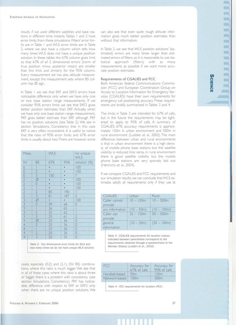
70

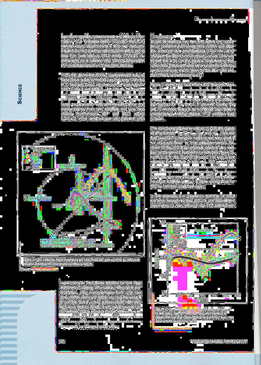
71

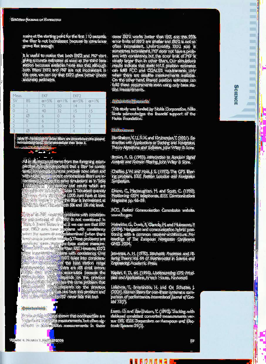
72

73

74 PUBLICATION 2 Simo Ali-Löytty and Niilo Sirola: A modified Kalman filter for hybrid positioning. In Proceedings of the 19th International Technical Meeting of the Satellite Division of the Institute of Navigation (ION GNSS 2006), Fort Worth TX, September 2006, pages

75

76 A Modified Kalman Filter for Hybrid Positioning Simo Ali-Löytty and Niilo Sirola, Institute of Mathematics, Tampere University of Technology, Finland BIOGRAPHY Simo Ali-Löytty is a Ph.D. student at Tampere University of Technology. He received his M.Sc. degree in 2004 from the same university. His research interest is filters in personal positioning. Niilo Sirola received his M.Sc. degree from Tampere University of Technology in He has been studying positioning algorithms since 2000, and is currently working on his Ph.D. thesis on novel mathematical methods for personal positioning and navigation. ABSTRACT This paper presents a new hybrid positioning algorithm whereby restrictive information such as base station sector and maximum range can be used in a Kalman-type filter. This new algorithm is fast to compute and gives almost the same accuracy as the particle filter with millions of particles. Simulations show that in some cases restrictive information such as mobile phone network sector and maximum range information dramatically improve filter accuracy. We also present the mathematical fundamentals of the algorithm. 1 INTRODUCTION Hybrid positioning means that measurements used in positioning come from many different sources e.g. Global Navigation Satellite System (GNSS), Inertial Measurement Unit (IMU), or local wireless networks such as a cellular network, WLAN, or Bluetooth. Range, pseudorange, deltarange, altitude, and compass measurements are typical measurements in hybrid positioning. Restrictive information can be used in positioning. By restrictive information, we mean the knowledge that the state e.g. position, is inside some area, which is the most often a polyhedron. In the simplest case, the area is a half-space. Base station sector and maximum range information (Cell ID) are examples of restrictive information [17]. Filters are used to compute an estimate of the state using current and past measurement data. Filters also give an approximation of the error covariance matrix. Kalmantype filters approximate the probability distribution of the state as a Gaussian or as a mixture of Gaussians. Extended Kalman Filter (EKF) [8, 10], Second Order Extended Kalman Filter (EKF2) [2], Unscented Kalman Filter (UKF) [9] and Gaussian Mixture Filter (GMF) [16, 7] are examples of Kalman-type filters. Maybe the most popular example is EKF, which is very commonly used in satellite-based positioning and has also been applied to hybrid positioning. Unfortunately, EKF has a serious consistency problem in highly nonlinear situations [1], i.e. the error covariance matrix is sometimes grossly underestimated. Contrary to satellite based positioning, highly nonlinear situations are common in hybrid positioning. Because of this, many researchers have investigated the use of general nonlinear Bayesian filter, which is usually implemented as a particle filter (SMC, Sequential Monte Carlo) [6, 13] or a point mass based filter [4, 14]. These filters usually work correctly and give good positioning accuracy but require much computation. An outline of the paper is as follows. After problem formulation in Section 2, the basic idea of the new algorithm is presented in Section 3. Section 4 provides the mathematical fundamentals of the algorithm. In Section 5, we concentrate on hybrid positioning application and illustrate how the new algorithm works in practice with sector and maximum range information. Finally, simulation results are given in Section 6. We show in Section 6 that in some cases the new hybrid positioning algorithm gives almost the same accuracy as a particle filter. In addition, the new algorithm avoids most of the consistency problems that plague the traditional EKF. The biggest advantage of the new algorithm is that it can use restrictive information and still needs notably less computation time than a particle filter. Because of this, it is conceivable that the algorithm can be implemented in a mobile device such as a mobile phone. 1679

77 2 BAYESIAN FILTERING We consider the discrete-time non-linear non-gaussian system x k = f k 1 (x k 1 ) + w k 1, (1) y k = h k (x k ) + v k, (2) where the vectors x k R nx and y k R ny k represent the state of the system and the measurement at time t k, k N, respectively. We assume that errors w k and v k are white, mutually independent and independent of the initial state x 0. The aim of the filtering is to find conditional probability density function (posterior) p(x k y 1:k ), (3) where y 1:k = {y1,..., y k }. Posterior can be determined recursively according to the following relations. Prediction: p(x k y 1:k 1 ) = p(x k x k 1 )p(x k 1 y 1:k 1 )dx k 1 ; Update: p(x k y 1:k ) = (4) p(y k x k )p(x k y 1:k 1 ) p(yk x k )p(x k y 1:k 1 )dx k, (5) where the transition pdf p(x k x k 1 ) can be derived from (1) and the likelihood p(y k x k ) can be derived from (2). The initial condition for the recursion is given by the pdf of the initial state p(x 0 y 1:0 ) = p(x 0 ). Knowledge of the posterior distribution enables one to compute an optimal state estimate with respect to any criterion. For example, the minimum mean-square error (MMSE) estimate is the conditional mean of x k [2, 13]. In general and in our case the conditional probability density function cannot be determined analytically. Because of this, there are many approximative solutions of conditional mean. Some popular Kalman-type approximative solutions of conditional mean include: PKF (Position Kalman Filter) works by filtering a sequence of static position and velocity solutions [1]. The idea is that we first solve position and velocity and then filter them; this idea is called two-stage estimator [5]. When we have enough measurements, we can find position and velocity for example by Weighted Least Squares (WLS) or closed-form methods [15]. WLS also approximates the errors of the solution. At time instants when there are not enough measurements to fix position and velocity, PKF does not use any measurements. 2.1 Restrictive information As we have seen, in the underdetermined case sometimes we have situation that posterior is multimodal and that can inflict inconsistency [1]. However, sometimes we have some extra information which may remove the multimodality. We call this extra information restrictive information. As mentioned previously, it is very common that we have restrictive information in hybrid positioning. For example, a mobile phone network, WLAN and Bluetooth base stations have specific range and if we hear the base station then we are inside the base station range. Of course restrictive information can also restrict other state variables than only position. More formally, restrictive information is measurement with measurement function (2) { 1, if x A h(x) = 0, if x / A, (6) where A R nx. In this paper, we consider only a case where restrictive information does not have error, so then error term v = 0 is constant random variable. The likelihood function of restriction information is characteristic function (5), (6) { 1, if x A p(1 x) = χ A (x) = 0, if x / A, (7) and respectively p(0 x) = χ A (x), where A is the complement of A. Unfortunately, it is not straightforward to use restrictive information with Kalman-type filters because measurement is a dichotomy variable and the measurement function is not linear. EKF (Extended Kalman Filter) Kalman filtering applied to a linearization of system (1), (2). EKF is very commonly used in satellite-based positioning and it has also been applied in hybrid positioning [10]. The EKF algorithm is described for example in [2, 8]. EKF2 (Second Order Extended Kalman Filter) an elaboration of EKF that models nonlinearity better. Modified Gaussian Second Order Filter [8, 12] is the same as EKF2. The EKF2 algorithm is given for example in [2]. 3 NEW ALGORITHM IN A NUTSHELL The main idea of the new algorithm is that we use some Kalman-type filter and extend it to use restrictive information. Here we present the new algorithm in the case where posterior is Gaussian, for example EKF, EKF2, PKF. 1. Compute the posterior without restrictive information using Kalman-type filter. 1680

78 2. If there is new restrictive information, model restrictive information as a likelihood function that is one inside a certain polyhedron and zero outside. 3. Compute new mean and covariance estimates. 4. Approximate the posterior distribution with a Gaussian, with the new mean and covariance. 5. Repeat this every timestep. The heart of this algorithm is stage 3, where we update posterior mean and covariance. Notice that this algorithm does not require any other measurements, so the algorithm works also if there is only restriction information. We can apply this algorithm also when posterior is Gaussian mixture. In this case, we apply this algorithm to every mixture component, and finally compute new mixture weights. 4 DERIVATION OF THE ALGORITHM In this section, we concentrate on the mathematical fundamentals of the new algorithm. First of all, the algorithm changes only the update part (5) so prediction part (4) remains the same as in the ordinary filter. 1. Compute the posterior without restrictive information using Kalman-type filter. Because of the independence, we can write likelihood function as the product p(y k x k ) = χ A (x k )p(y k x k ), (8) where A is the intersection of all new restrictive information, this means that state is inside A at time instant t k and y k are other measurements than restrictive information at time instant t k. Using Eqs. (5) and (8) we find that where p(x k y 1:k) = p(x k y 1:k ) χ A (x k )p(x k y 1:k ), (9) p(y k x k)p(x k y 1:k 1 ) p(y k x k )p(x k y 1:k 1 )dx k (10) is posterior without current restrictive information. This can be computed using the ordinary Kalman-type filter. We use notation that µ old and Σ old represent the approximations of the mean and the covariance matrix of this distribution, respectively. We also approximate p(x k y 1:k ) with a Gaussian. 2. If there is new restrictive information, model restrictive information as a likelihood function that is one inside a certain polyhedron and zero outside. We use the same restrictive information only once within a certain time period, because otherwise our approximation error can accumulate and cause unwanted phenomena. Let the area A be inscribed in the polyhedron (see Fig 1) b T B = x 1. x β = {x Bx β}, (11) b T n where matrix B is organized so that the first inequality reduces probability the most, that is p(x k y 1:k )dx k p(x k y 1:k )dx k b T 1 xk β1 b T n xk βn β 1 b T 1 µ old b T 1 Σ old b 1 β n b T n µ old. b T n Σ old b n (12) We use Gram-Schmidt orthonormalization on {b 1,..., b n } with inner product < x, y >= x T Σ old y, and get matrix A whose row space is same than the row space of matrix B and AΣ old A T = I. Now we approximate the likelihood of restrictive information with one inside the polyhedron (see Fig 1) A = {x Ax Ax mid α} (13) and zero elsewhere. So we replace χ A in Eq. (9) with χ A. Vectors Ax mid and α we select so that B is subset of A and probability that state is inside A is as small as possible. Then also A is subset of A. If X = [ x 1,..., x N ] are vertices of polyhedron B, then and where and α = up low 2 Ax mid = Aµ old (14) (15) up + low, (16) 2 up = Aµ old min (AXe i) (17) i {1,...,N} low = Aµ old max (AXe i). (18) i {1,...,N} Operators min and max are taken separately with every components. We use this same notation through the paper. 3. Compute new mean and covariance estimates. In this stage, we compute the approximation of the mean µ new and the covariance matrix Σ new of the modified posterior p(x k y 1:k ) (9), where A is replaced with A. This approximation is accurate if the old posterior p(x k y 1:k ) 1681

79 is Gaussian and A = A. First we compute probability that state is inside polyhedron A, p new = χ A (x k )p(x k y 1:k)dx k = p z (z)dz (19) z α n = (Φ (up i ) Φ (low i )), i=1 where Φ (x) is cumulative density function (cdf) of x, when x N(0, 1). The idea of the solution is that with the change variables, z = Ax k Ax mid, E(z) = µ z = Aµ old Ax mid, V(z) = Σ z = AΣ old A T = I, (20) we can compute the integral iteratively. We use this same idea also in the following integrals, when computing mean and covariance matrix. If posterior is Gaussian mixture then the new weight is proportional to old weight times the probability p new. The approximation of the mean of the posterior distribution p(x k y 1:k ) is where and ǫ = χ A (x k )p(x k y 1:k µ new = x ) k dx k p new = A 1 zp z (z)dz + x mid p new z α = A 1 zp z (z)dz + x mid (35) = µ old + Σ old A T ǫ (21) p z (z) = χ z α(z)p z (z) p new (22) ) ) n exp ( upi2 2 exp ( lowi2 2 e i. (23) 2π (Φ (upi ) Φ (low i )) i=1 Details of the computation are given in Appendix A, Eq. (35). Here we assumed that A R na ma is square matrix (n A = m A ) and non-singular, so polyhedron A is a bounded box. Now we show that Eq. (21) holds also when we have an unbounded area. If n A < m A we can add more rows to matrix A and elements to vector α, this means that we add more restrictive information. When the added elements α i, i {n A,..., m A } tend to infinity, we get same equation as previously, because ǫ i, i {n A,..., m A } go to zero. The approximation of the covariance matrix of the posterior distribution p(x k y 1:k ) is Σ new = (x k µ new )(x k µ new ) T χ A (x k)p(x k y 1:k ) dx k p new = A 1 (z µ z )(z µ z ) T p z (z)dza T where where (37) = A 1 (I Λ)A T = Σ old Σ old A T ΛAΣ old, (24) µ z = µ z + ǫ = Aµ new Ax mid, (25) Λ = diag(δ) + diag(ǫ) diag(aµ new Ax mid ), (26) δ = ) ( ) n exp 2 + exp lowi2 2 α i e i. (27) 2π (Φ (upi ) Φ (low i )) i=1 ( upi2 Details of the computation are given in Appendix A, Eq. (37). This equation also works when matrix A is not a square matrix. Proof goes similarily than previously. 4. Approximate the posterior distribution with a Gaussian, with the new mean and covariance. This stage usually produces the most approximation errors in this algorithm. This is the reason why we use each restrictive information only once. 5. Repeat this every timestep. 5 EXAMPLE OF THE NEW ALGORITHM In this section, we illustrate how the new algorithm works. In this example, Fig 1, restrictive information consists of two base station Cell IDs, which means that we know the base stations sector and maximum range information. In the figure, dark area (area A in Eq. (9)) is the intersection of these information and so we know that user is inside this area. Black dashed polyhedron represents an polyhedron approximation of the true restrictive area (11). Black solid polyhedron represents the certain polyhedron approximation of the polyhedron approximation of the true restrictive area (13). Red man stands on prior mean and a red dashed ellipse represent prior covariance. The covariances (Σ) are visualized with ellipses that satisfy the equation (x µ) T Σ 1 (x µ) = (28) The constant was chosen so that if the distribution is Gaussian then there is 67% probability mass inside the ellipse. Respectively, blue man stands on posterior mean and a blue solid ellipse represent posterior covariance. 1682

80 Prior Posterior Polyhedron B (11) Polyhedron A dot (13) t k = t k t k 1, and w k 1 is white, zero mean and Gaussian noise, with covariance matrix t 3 k σ2 p t 3 I 0 2 k σ2 p 2 I 0 t Q k 1 = 0 3 k σ2 a t k σ2 a 2 t 2 k σ2 p t kσ 2 I 0 2 p 1 I 0, (31) 0 t 2 k σ2 a 2 0 t kσ 2 a 1 Base station 500 m where σp 2 = 2 m2 s represents the velocity errors on the East- 3 North plane and σa 2 = 0.1 m2 s represents the velocity errors 3 in the vertical direction. [11, 1] In our simulations, we use base station range measurement, altitude measurement, satellite range measurement and satellite deltarange measurement. Figure 1: Red means prior distribution. Dashed black polyhedron represents the first approximation of restrictive area (11). Solid black polyhedron represents the certain approximation of the true restrictive area (13). Blue represents the mean and covariance approximations after applying the restrictive information. It is quite evident that using restrictive information improves estimates notably only when there is much probability mass outside the restrictive area. Usually, this happens two different cases. The first case is that we have only a few measurement, which causes large posterior covariance without restrictive information, but we have quite good restrictive information such as sector information. Other possibly is that Kalman-type filters works totally wrong, this means that filter is inconsistent so that predicted errors are smaller than actual errors [1]. Both of these cases are possible in hybrid positioning, so it is reasonable to use restrictive information in hybrid positioning. In Section 6, we see more specifically how restrictive information improves Kalman-type filter performance in hybrid positioning. 6 SIMULATIONS In the simulations, we use the position-velocity model, so the state x = [ r T u, ] T vt u consists of user position vector ru and user velocity vector v u, which are in East-North-Up (ENU) coordinate system. In this model the user velocity is a random walk process [3]. Now the state-dynamic Eq. (1) is where x k = Φ k 1 x k 1 + w k 1, (29) [ ] I tk I Φ k 1 =, (30) 0 I y b = r b r u + ǫ b, y a = [ ] r u + ǫ a, y s = r s r u + b + ǫ s, ẏ s = (r s r u ) T r s r u (v s v u ) + ḃ + ǫ s, (32) where r b is base station position vector, r s is satellite position vector, b is clock bias, v s is satellite velocity vector, ḃ is clock drift and ǫ:s are error terms. We use satellite measurements only when there is more than one satellite measurement available, so that bias can be eliminated. These are the same measurements equations as in the paper [1]. Restrictive information that we use are base station sector information and maximum range information. From Fig. 2, we get an idea of how the new algorithm works. These simulations use only a few (one or two at the same time instant) base station range measurements with variance (100 m) 2 and altitude measurement with variance (300 m) 2. In this case, restrictive information keeps the filter always consistent (not inconsistent). In this paper, we use the general inconsistency test, with risk level 5% [1]. Restrictive information also decreases the mean error from 442 meters to 93 meters. In Table 1, we have listed a summary of a hundred 300 second simulations. The simulations use only a few (one or two at the same time instant) base station range measurements with variance (80 m) 2 and altitude measurements with variance (300 m) 2. Summary consist of following columns: Time is relative computation time using Matlab and our implementation, so that computation time of EKF is one. This is not entire truth, but gives an idea of complexity of each algorithm. Err. µ is 2D position error mean. Err. 95% tells that 95 % errors are less than this limit. Err. ref. is 2D error to reference posterior mean, which is computed using particle filter with particles. Err. <50 is how many percentage of times 2D position error is less than 50 meter. Inc. % is how many percentage of time filter is inconsistent with respect to the general inconsistency test, with risk level 5% [1]. Solvers are organized so that mean positioning errors are in descending order. We also test 1683

81 500 m True track EKF EKF with restrictive info Start Base station Figure 2: This figure illustrate how the new algorithm, EKF with restrictive information (EKFBOX), improve EKF in mobile phone positioning. In this case EKF and EKFBOX mean of the position errors are 442 m and 93 m, respectively. positioning using only restrictive information, we call this the BOXsolver. We also use BOX suffix when we use the new algorithm for incorporating restrictive information. Table 1: Summary of 100 different simulations with very poor geometry. Simulations only use a few base station range measurements and very inaccurate altitude measurements; an example of this geometry is in Fig. 2. Time Err. Err. Err. Err. Inc. Solver µ 95% ref <50 % EKF EKF BOX EKFBOX EKF2BOX SMC Ref From Table 1, we see that restrictive information improves greatly filters performance. Every statistic, except CPU time, of the Kalman-type filters is improved by the new algorithm. Also, difference between the reference solution (particle filter), which uses all restrictive information, and EKF(2)BOX-solver is quite small. However EKF(2)BOXsolver s computation time is much less than the particle filter (SMC). SMC and reference solvers are the same solver, but SMC solver uses 10 4 particles, when reference solves uses 10 6 particles. Note that the geometry is quite bad and traditional solvers like EKF(2) give even worse results than BOX-solver, which uses only restrictive information and not range measurements or altitude measurements at all. In Table 2 we have listed a summary of a hundred simulations, but now simulations use normal suburban geometry. This means that simulations use few base station range measurements, very inaccurate altitude measurements, some (not more than five) satellite pseurange and delta pseudorange measurements, with variance (20 m) 2 and (2 m s )2 respectively. We see that errors are smaller, of course, than in Table 1. If we concentrate on the error ratio of different filters, we see that results are quite same than previosly. So the new algortihm improves Kalman-type filters much and these EKF(2)BOX-solvers give almost the same accuracy as particle filters. Table 2: Summary of 100 different simulations with normal suburban geometry. Simulations use few base station range measurements, very inaccurate altitude measurements, some satellite pseurange and delta pseudorange measurements. Time Err. Err. Err. Err. Inc. Solver µ 95% ref <50 % BOX EKF EKF EKFBOX EKF2BOX SMC Ref CONCLUSIONS We presented a new hybrid positioning algorithm, which makes possible to use restrictive information with Kalmantype filters. The new algorithm needs clearly less computation time than the general nonlinear Bayesian filters such as the particle filter with 10 4 particles. Simulations show that the new algorithm is very well suited to hybrid positioning application, where we have sector and maximum range restrictive information. In this application, the new algorithm improves EKF and EKF2 much and gives almost same accuracy as reference particle filters. 1684

82 A AUXILIARY INTEGRALS In this section, we compute some auxiliary integrals. Here z is n z -dimensional Gaussian random variable with mean µ z and covariance matrix is identity matrix. So the density function of z is and so n z n z exp p z (z) = p zi (z i ) = i=1 i=1 ( (zi µz i )2 2 ) 2π (33) Σ z = (z µ z )(z µ z ) T p z (z)dz n z = e j e T j (z j µ z j ) 2 p z (z)dz n z = e j e T j (z j µ zj ǫ j ) 2 p z (z)dz n z = e j e T j (z j µ zj ) 2 p z j (z)dz j diag(ǫ) 2 = I diag(δ) diag(ǫ) diag(aµ new Ax mid ) (37) p z (z) = χ z α(z)p z (z) p new ) n z χ zi α i (z i ) exp ( (zi µz i )2 2 = (Φ (up i ) Φ (low i )) 2π i=1 n z = p z i (z i ), i=1 (34) ACKNOWLEDGMENTS This study was partly funded by Nokia Corporation. Simo Ali-Löytty acknowledges the financial support of the Nokia Foundation and the Tampere Graduate School in Information Science and Engineering. The particle filter we used was implemented by Duane Petrovich. which is also a density function. Auxiliary integral of derivation of Eq. (21) µ z = = zp z (z)dz n z (z µ z ) p z i (z i )dz + µ z i=1 n z n z = e j (z j µ zj ) p z i (z i )dz + µ z i=1 n αj z α = e j (z j µ zj )p zj (z j )dz j j + µ z Φ (up j ) Φ (low j ) ( ) ( ) n z exp up2 j 2 exp low2 j 2 = e j + µ z 2π (Φ (upj ) Φ (low j )) = ǫ + µ z, (35) where p new is defined in Eq. (19) and from Eqs. (15), (16) and (20) we get that up = µ z + α and low = µ z α. (36) Auxiliary integral of derivation of Eq. (24) REFERENCES [1] S. Ali-Löytty, N. Sirola, and R. Piché. Consistency of three Kalman filter extensions in hybrid navigation. In Proceedings of The European Navigation Conference GNSS 2005, Munich, Germany, July [2] Y. Bar-Shalom, R. X. Li, and T. Kirubarajan. Estimation with Applications to Tracking and Navigation, Theory Algorithms and Software. John Wiley & Sons, [3] R. G. Brown. Introduction to Random Signal Analysis and Kalman Filtering. John Wiley & Sons, [4] R. S. Bucy and K. D. Senne. Digital synthesis of nonlinear filters. Automatica, 7(3): , May [5] J. W. Chaffee and J. S. Abel. The GPS filtering problem. IEEE Position Location and Navigation Symposium, [6] A. Doucet, N. de Freitas, and N. Gordon, editors. Sequential Monte Carlo Methods in Practice. Statistics for Engineering and Information Science. Springer, [7] K. Ito and K. Xiong. Gaussian filters for nonlinear filtering problems. IEEE Transactions on Automatic Control, 45(5): , May [8] A. H. Jazwinski. Stochastic Processes and Filtering Theory, volume 64 of Mathematics in Science and Engineering. Academic Press,

83 [9] S. J. Julier and J. K. Uhlmann. Unscented filtering and nonlinear estimation. Proceedings of the IEEE, 92(3): , March [10] C. Ma. Integration of GPS and cellular networks to improve wireless location performance. Proceedings of ION GPS/GNSS 2003, pages , [11] P. S. Maybeck. Stochastic Models, Estimation, and Control, volume 141 of Mathematics in Science and Engineering. Academic Press, [12] P. S. Maybeck. Stochastic Models, Estimation, and Control, volume of Mathematics in Science and Engineering. Academic Press, [13] B. Ristic, S. Arulampalam, and N. Gordon. Beyond the Kalman Filter, Particle Filters for Tracking Applications. Artech House, Boston, London, [14] N. Sirola and S. Ali-Löytty. Local positioning with parallelepiped moving grid. In Proceedings of 3rd Workshop on Positioning, Navigation and Communication 2006 (WPNC 06), pages , Hannover, March 16th [15] N. Sirola, R. Piché, and J. Syrjärinne. Closedform solutions for hybrid cellular/gps positioning. Proceedings of ION GPS/GNSS 2003, pages , [16] H. W. Sorenson and D. L. Alspach. Recursive Bayesian estimation using Gaussian sums. Automatica, 7(4): , July [17] M. A. Spirito, S. Pöykkö, and O. Knuuttila. Experimental performance of methods to estimate the location of legacy handsets in GSM. IEEE Vehicular Technology Conference, pages ,

84 PUBLICATION 3 Simo Ali-Löytty and Niilo Sirola: Gaussian mixture filter in hybrid navigation. In Proceedings of the European Navigation Conference 2007 (ENC 2007), Geneva, May 2007, pages

85

86 Gaussian Mixture Filter in Hybrid Navigation Simo Ali-Löytty and Niilo Sirola, Institute of Mathematics, Tampere University of Technology, Finland BIOGRAPHY Simo Ali-Löytty is a Ph.D. student at Tampere University of Technology. He received his M.Sc. degree in 2004 from the same university. His research interest is filters in personal positioning. Niilo Sirola is a Ph.D. student at Tampere University of Technology. He received his M.Sc. degree in 2003 from the same university. He began his research on personal positioning algorithms in ABSTRACT This paper studies the Gaussian Mixture Filter (GMF) in hybrid navigation and is divided into three parts focusing on different problems. The first part deals with approximating the likelihood function as a Gaussian mixture. The second part gives a new way to robustify GMF by adding more components, and the third part concentrates on different ways to reduce the number of mixture components so that the algorithm is fast without losing significant information. Finally, we compare GMF with other filters using simulations. 1 INTRODUCTION Hybrid navigation means navigation using measurements from different sources e.g. Global Navigation Satellite System (e.g. GPS), Inertial Measurement Unit, or local wireless networks such as a cellular network, WLAN, or Bluetooth. Range, pseudorange, deltarange, altitude, restrictive and compass measurements are examples of typical measurements in hybrid navigation. The most popular example of navigation filters is the Extended Kalman Filter (EKF), which linearizes system and measurement models and then applies the traditional Kalman Filter [6, 9]. EKF is commonly used in satellite based positioning and has also been applied to hybrid navigation [11]. Unfortunately, EKF has a serious consistency problem in highly nonlinear situations, which means that EKF does not work correctly [2]. In highly nonlinear situations, we sometimes have multiple static position solutions, which means that likelihood function has multiple peaks with significant weight. In this case, it is more reasonable 831 to approximate the likelihood as a Gaussian mixture and use GMF (section 4) than to approximate with only one Gaussian as the EKF does. We present a new method to robustify the GMF in section 5, which takes into consideration that the prior distribution might be wrong. This is usually the case when the filter has inconsistency problems. In a nutshell, the idea of the new method is following: if measurements are unlikely with respect to the prior, the new method adds mixture components so that the new mixture consists of the prior or posterior distribution plus extra component(s) that are approximately proportional to the likelihood function. This is better than the traditional robust approach which can discard good measurements because an erroneous prior makes them seem unlikely. The proposed method does not replace old methods but rather extends them. One major challenge in using GMF efficiently is keeping the number of components as small as possible without losing significant information. We study in section 6 both the traditional component reduction methods, merging and forgetting, and new resampling algorithms similar to the ones used in particle filters. In the simulations part in section 7, we compare different GMFs with different Kalman type filters such as EKF and the Unscented Kalman Filter (UKF) [10], as well as with a bootstrap particle filter [4]. We compare the mean estimates given by the filters to the true track and to the mean estimate of the nearly optimal particle filter. We also look at the computation times and different inconsistency statistics. It is interesting to notice that none of the filters dominate with respect to all of the criteria, so with suitable weighting of the criteria we could make any of the filters win the comparison. However, generally it is possible to develop GMF which works better than EKF or UKF especially when we consider a robust viewpoint. Naturally GMF needs more computations than EKF or UKF but usually less than the particle filter. 2 BAYESIAN FILTERING We consider the discrete-time non-linear non-gaussian system x k = f k 1 (x k 1 ) + w k 1, (1) y k = h k (x k ) + v k, (2)

87 where the vectors x k R nx and y k R ny k represent the state of the system and the measurement at time t k, k N, respectively. We assume that errors w k and v k are white, mutually independent and independent of the initial state x 0. We denote the density functions of w k and v k by p wk and p vk, respectively. The aim of filtering is to find the conditional probability density function (posterior) p(x k y 1:k ), where y 1:k = {y1,..., y k }. The posterior can be determined recursively according to the following relations. Prediction (prior): p(x k y 1:k 1 ) = p(x k x k 1 )p(x k 1 y 1:k 1 )dx k 1 ; Update (posterior): p(x k y 1:k ) = where the transition pdf is (3) p(y k x k )p(x k y 1:k 1 ) p(yk x k )p(x k y 1:k 1 )dx k, (4) p(x k x k 1 ) = p wk 1 (x k f k 1 (x k 1 )) and the likelihood p(y k x k ) = p vk (y k h k (x k )). (5) The initial condition for the recursion is given by the pdf of the initial state p(x 0 y 1:0 ) = p(x 0 ). Knowledge of the posterior distribution (4) enables one to compute an optimal state estimate with respect to any criterion. For example, the minimum mean-square error (MMSE) estimate is the conditional mean of x k [6, 17]. In general and in our case, the conditional probability density function cannot be determined analytically. 3 GAUSSIAN MIXTURE FILTER We assume that the prior (3) and likelihood (5) are p p(x) = α i N µi Σ i (x) and p(y x) = i=1 m β j N Hjx R (y). Then the posterior is a Gaussian mixture (see appendix A) m p i=1 α iβ j N Hjµi P i,j (y) Nˆxi,j (x) ˆP p(x y) = i,j m p i=1 α, (7) iβ j N Hjµi P i,j (y) where P i,j = H j Σ i H T j + R, ˆx i,j = µ i + K i,j (y H j µ i ), ˆP i,j = (I K i,j H j )Σ i and K i,j = Σ i H T j P 1 i,j. 4 GAUSSIAN MIXTURE APPROXIMATION OF LIKELIHOOD Henceforth we assume that errors w k and v k are zeromean Gaussian with covariance matrix Q k and R k, respectively. Also we assume that the initial state x 0 is a Gaussian mixture and that the state model (1) is linear so f k 1 (x k 1 ) = Φ k 1 x k 1. If the posterior density p(x k y 1:k ) is a Gaussian mixture (6) then the next prior density (3) is (see appendix A (11)) p p(x k+1 y 1:k ) = α i N Φkxk Q k (x k+1 ) N µi Σ i (x k )dx k = i=1 p i=1 α i N Φkµi Φ kσ iφ T k +Qk (x k+1 ), which is also a Gaussian mixture. So the actual problem is how to approximate/compute the new posterior density (4), that is, how to approximate the product The idea of GMF [3] is that both prior density (3) and posterior density (4) are Gaussian mixtures p(x) = p i=1 α i N µi Σ i (x), (6) where N µi Σ i (x) is the normal density function with mean µ i and covariance matrix Σ i. Weights are non-negative and sum to one. The mean of a Gaussian mixture (6) is and the covariance Σ = µ = p α i µ i i=1 p α i (Σ i + (µ i µ)(µ i µ) T ). i=1 832 p(x k y 1:k ) p(y k x k )p(x k y 1:k 1 ), where (see (5)) ( ) exp 1 2 y k h k (x k ) 2 R p(y k x k ) = 1 k det(2πrk ) and y k h k (x k ) 2 R 1 k = (y k h k (x k )) T R 1 k (y k h k (x k )). There are many possibilities to do this. We can use the same methodology that Kalman filter extensions use to get GMF EKF Extended Kalman Filter (EKF) [6, 9], linearize the measurement function around the prior mean ˆx k k 1 h k (x k ) h k (ˆx k k 1 ) + h k (ˆx k k 1)(x k ˆx k k 1 ).

88 GMF EKF2 Second Order Extended Kalman Filter [9] is an elaboration of EKF that models nonlinearity better. Modified Gaussian Second Order Filter [14] is the same as EKF2. GMF UKF Unscented Kalman Filter [10] is based on the numerical integration method called the unscented transformation. Often these are quite good approximations, but sometimes especially when likelihood has several peaks in a neighbourhood of the prior mean, these approximations fail. These are actually situations where the above filters and other unimodal Kalman filter extensions can easily have consistency problems. Because of this, we develop a new approximation that works better in this situation. First we compute (see appendix B) z = argmin xk [ (yk h k (x k )) T R 1 k (y k h k (x k ) ], (8) which is possibly ambiguous, so we denote the minimizers z 1,..., z m. We consider only the situation where there is a finite number of minimum points. Then we approximate ( ) m exp 1 2 ỹ k H kj x k 2 R p(y k x k ) 1 k, (9) det(2πrk ) where H kj = h k (z j) and ỹ k = y k h k (z j ) + H kj z j. This approximation ensures that the posterior is also a Gaussian mixture, and takes into consideration the possibility that the likelihood has multiple peaks. An other benefit is that this approximation is independent of prior mean, so it is quite good even if the prior is totally wrong. This is a very important feature when we study the robustness of the GMF. We use this approximation in two different ways GMF new1 approximate the likelihood as a Gaussian mixture (9) when we find that the likelihood has one or more peaks. When there is an infinite number of peaks or we do not find any peaks, GMF new1 works like GMF EKF. GMF new2 approximate the likelihood as a Gaussian mixture (9) only when we find that the likelihood has a finite number and more than one peak, otherwise GMF new2 works like GMF EKF. approximate likelihood function and thus do not depend on the prior information. If we assume that the prior is possibly wrong, it is justified to add components approximating likelihood function, because likelihood is proportional to posterior if we have constant prior (prior density with very large covariance). Other components might be appropriately scaled posterior components or prior components. Next we elaborate on the unlikeliness of measurements. We know that p(y k y 1:k 1 ) = p(y k x k )p(x k y 1:k 1 )dx k. Now substitute the prior p(x k y 1:k 1 ) = p i=1 α i N µi Σ i (x k ) and the approximate likelihood (9) to obtain (compare to (7)) p(y k y 1:k 1 ) = m p i=1 which is also a Gaussian mixture where α i N µi,j Σ i,j (y k ), µ i,j = h k (z j ) + H kj (µ i z j ) and Σ i,j = H kj Σ i H T k j + R k. Furthermore, ( ) P y k µ i,j 2 > a Σ 1 th, i, j i,j < p ath, (10) where a th χ 2 n yk (x)dx = p ath, χ 2 n yk (x) is density function of χ 2 (n yk )-distribution. So now measurements are unlikely if y k µ i,j 2 > a Σ 1 th, i, j, i,j where a th is some threshold parameter that is a function of the risk level p ath. 6 COMPONENTS REDUCTION 5 NEW WAY TO ROBUSTIFY GMF Many robust filters are based on using innovation y k h k (x k ) such that too big innovations are downweighted or the corresponding measurement discarded [8, 12, 16]. These approaches assume that the prior is correct, which is not always true. We present a new heuristic to robustify GMF. This method does not replace old methods but complements them, because we can use both methods at same time. If measurements are unlikely (see (10)), we will add new components with appropriate weights. These new components 833 One major challenge in using GMF efficiently is keeping the number of components as small as possible without losing significant information. There is many ways to do so. We use three different types of mixture reduction algorithms: forgetting, merging and resampling. Forgetting Give zero weight to mixture components whose weights are lower than some threshold value, for example ( min 0.001, 0.01 max i ) (α i ). After that, normalize weights of the remaining mixture components.

89 Merging Merge two mixture components to one if distance between components is lower than some threshold value. Distance is for example [18] d ij = α iα j α i + α j (µ i µ j ) T Σ 1 (µ i µ j ). Merge components so that merging preserves the overall mean and covariance. This method, collapsing by moments, is optimal in the sense of Kullback-Leibler distance [15]. Resampling If after forgetting and merging there are too many mixture components, we can use a resampling algorithm to choose which mixture components to keep, then normalize the weights of these mixture components. This approach induces less approximation error, using L 1 -norm, than merging two distant components. 7 SIMULATIONS In the simulations, [ we ] use the position-velocity model, so ru the state x = consists of user position vector r v u u and user velocity vector v u, which are in East-North-Up (ENU) coordinate system. In this model the user velocity is a random walk process [7]. Now the state-dynamic Eq. (1) is where x k = Φ k 1 x k 1 + w k 1, [ ] I tk I Φ k 1 =, 0 I vector, ḃ is clock drift and ǫ:s are error terms. We use satellite measurements only when there is more than one satellite measurement available, so that bias can be eliminated. These are the same measurements equations as in the papers [2, 1]. 7.1 Example where GMF beats EKF As mentioned before, EKF has a serious consistency problem in highly nonlinear situations, which means that EKF does not work correctly [2]. One example of highly nonlinear situations is shown in Fig. 1, where we have only range measurements from two base stations. In this case EKF s estimate veers away from the true route and gets stuck in an incorrect solution branch. GMF, which approximates likelihood as a Gaussian mixture (see (9)) finds both peaks of the posterior function. So in this case we can say that GMF works better than EKF. Nevertheless, it is important to notice that before EKF select the incorrect solution branch it gives better estimates than GMF. This is because prior mean, which is the linearization point of EKF, is usually a better state estimate than likelihood peaks, around which GMF is linearized. Thus EKF usually gives smaller 2D root-mean-square position error than the variant of GMF that always uses likelihood peak(s) as linearization points (see section (7.2)). True EKF GMF mean GMF components t k = t k t k 1, and w k 1 is white, zero mean and Gaussian noise, with covariance matrix t 3 k σ2 p t 3 I 0 2 k σ2 p 2 I 0 t Q k 1 = 0 3 k σ2 a t k σ2 a 2 t 2 k σ2 p t kσ 2 I 0 2 p 1 I 0, 0 t 2 k σ2 a 2 0 t kσ 2 a 1 where σp 2 = 2 m2 s represents the velocity errors on the East- 3 North plane and σa 2 = 0.1 m2 s represents the velocity errors 3 in the vertical direction. [13, 2] In our simulations, we use base station range measurements, altitude measurements, satellite range measurements and satellite doppler measurements (see (2)). y b = r b r u + ǫ b, y a = [ ] r u + ǫ a, y s = r s r u + b + ǫ s, ẏ s = (r s r u ) T r s r u (v s v u ) + ḃ + ǫ s, where r b is a base station position vector, r s is a satellite position vector, b is clock bias, v s is a satellite velocity m Start Figure 1: One example where GMF beats EKF. Here true posterior has two peaks and GMF finds them but EKF selects incorrect solution branch. 7.2 Summary of suburban cases In Table 1, we have listed a summary of two hundred 120 second simulations, which use typical suburban geometry. This means that simulations use a few base station range measurements with variance (100 m) 2, inaccurate altitude measurements with variance (75 m) 2, some (not more than five) satellite pseudorange and doppler measurements, with variance (25 m) 2 and (2 m s )2 respectively. Summary consist of following columns: Time is computation time using Matlab in our implementation, scaled so that computation time of EKF is 1. This gives a rough idea of the time complexity of each algorithm. Err. rms

90 is 2D root mean square position error. Err. 95% gives a radius containing 95 % of the 2D errors. Err. ref. is 2D error to reference posterior mean, which is computed using a particle filter with 10 6 particles. Inc. % is percentage of time where filter is inconsistent with respect to the general inconsistency test, with risk level 5% [2]. Solvers are sorted so that rms errors are in descending order. Different GMF subscripts indicate how solvers make the updating step, see section 4. Every GMF variant adds components that approximate the likelihood whenever measurements are unlikely (see section 5). Also, every GMF variant keeps the number of mixture components very small (not more than eight) using component reduction (see section 6). PF 10 3 indicates particle filter with systematic resampling and 10 3 particles [4]. Table 1: Summary of 200 different simulations with typical suburban geometry. Simulations use a few base station range measurements, altitude measurements, some satellite pseudorange and doppler measurements. Time Err. Err. Err. Inc. Solver rms 95% ref % GMF new EKF UKF EKF GMF ekf GMF ukf GMF ekf GMF new PF Ref The following conclusions can be drawn based on simulations and theory. Even if GMF new2 gives better results (especially Err. 95%) than traditional GMFs such as EKF, there are still some inconsistency problems. 8 CONCLUSIONS In this article, we have studied three aspects of the Gaussian Mixture Filter: how to approximate the likelihood function as a Gaussian mixture, a heuristic method to robustify GMF by adding more components, and different ways to reduce the number of mixture components so that the algorithm is fast without losing significant information. We also compared GMFs with different filters using simulations. We test especially two Gaussian mixture filters that use a new way to robustify GMF, use at most eight mixture components and approximate likelihood as Gaussian mixture. GMF new2, which approximates likelihood as Gaussian mixture only when likelihood has more than one peak and otherwise computes updating step like EKF, works much better than EKF. GMF new1 is the same as GMF new2 except that it approximates likelihood as Gaussian mixture always when likelihood has peak(s). Simulations show that the GMF new2 works better than EKF, EKF2 or UKF, with respect to the estimation errors. However, GMF new1 gives larger errors than EKF. So this new method approximates likelihood as a Gaussian mixture, beats EKF actually only when EKF has possible problems e.g. posterior has multiple peaks. Simulations also show that robust GMF gives better results than basic GMF. A POSTERIOR OF GMF We assume that prior (3) is The new GMF robustifying heuristic (section 5) improves results a bit, even if simulated data does not have any outliers. That is, GMF EKF, GMF EKF2 and GMF UKF give better results than EKF, EKF2 and UKF, respectively. One reason for this is that there are some simulations where EKF, EKF2 and UKF are inconsistent and adding components which approximate the likelihood to GMF gives better results. GMF new1 has bigger errors than EKF, which indicates that it is not always reasonable to approximate likelihood as a Gaussian mixture. GMF new2 gives better results than other GMFs, especially GMF new1 and EKF. So it is reasonable to approximate likelihood as Gaussian mixture only when there is risk that posterior has multiple significant peaks, e.g. when likelihood has more than one peak. It seems that PF 10 3 gives better results than the GMFs, with simulated data without outliers. The basic PF 10 3 is not expected to work very well with real data. 835 and likelihood (5) is p(x) = p(y x) = Then the posterior is (4) (11) = p i=1 m α i N µi Σ i (x), β j N Hjx R (y). m p(x y) = β j N Hjx R (y) p i=1 α i N µi Σ i (x) m β j N Hjx R (y) p i=1 α i N µi Σ i (x)dx m p i=1 = α iβ j N Hjx R (y) Nµi Σ i (x) m p i=1 α H iβ j N jx R (y) Nµi Σ i (x)dx m p i=1 α iβ j N Hjµi P i,j (y) Nˆxi,j (x) ˆP i,j m p i=1 α iβ j N Hjµi P i,j (y),

91 where P i,j = H j Σ i H T j + R, ˆx i,j = µ i + K i,j (y H j µ i ), ˆP i,j = (Σ 1 i + H T j R 1 H j ) 1 = (I K i,j H j )Σ i and K i,j = Σ i H T j P 1 i,j. Here we use the fact that N Hjx R (y) Nµi Σ i (x) = exp ( 1 2 a ) 2 (n y+n x) 2π a1 where and = N Hjµi P i,j (y) Nˆxi,j (x), ˆP i,j a 1 = det(r) det(σ i ) ([ ]) Σi 0 = det 0 R ([ ] [ ] [ I 0 Σi 0 I H T = det j H j I 0 R 0 I ([ Σ i Σ i H T j = det ([ I Ki,j = det 0 I H j Σ i H j Σ i H T j + R ]) = det(p i,j ) det(ˆp i,j ) ] [ ˆPi,j 0 H j Σ i P i,j ]) ]) (11) Matrix R 1 is positive definite so (y h(r)) T R 1 (y h(r)) 0, and equality holds only when y = h(r). First, we try to find closed-form solutions z so that y = h(z) [20, 19, 5]. If we have only linear measurements we get z = ( H T R 1 H ) 1 H T R 1 y = argmin r [ (y Hr) T R 1 (y Hr) ], (13) if ( H T R 1 H ) 1 exists, otherwise we have an infinite number of solutions. If there is no closed-form solution and we have at least one range measurement we use iterative weighted least squares (IWLS) to find solution. The initial iterate z 0 for WLS-algorithm can be found, for example, by omitting some measurements and using the closed-form solution, see equation (13), or by one of the following closed-form equations, respectively. One range meas and two linear meas where r line = z = r line + n T line(r 1 r line )n line, [ n T line H ] 1 y, and n line = HT 1,: HT 2,: H T 1,: HT 2,:, a 2 = y H j x 2 R 1 + x µ i 2 Σ 1 i = x 2 H T j R 1 H j+σ 1 i + y 2 R 1 + µ i 2 Σ 1 i = x ˆx i,j 2ˆP 1 i,j + y 2 R 1 + µ i 2 Σ 1 i = x ˆx i,j 2ˆP 1 i,j 2(y T R 1 H j + µ T i Σ 1 i )x... H T j R 1 y + Σ 1 i µ i 2ˆPi,j... 2µ T i Σ 1 i + y 2 + µ P 1 i 2 i,j H T j P 1 i,j Hj = x ˆx i,j 2ˆP 1 i,j + y H j µ i 2. P 1 i,j ˆP i,j H T j R 1 y... where we assume that H T 1,: H T 2,: > 0. Here z is the point on a line r = r line +kn line, for which distance from sphere y 1 = r 1 r is minimum. This straight line does not intersect the sphere because we have assumption that we do not have closed-form solution. Two range meas and one linear meas We select our indices so that y 1 y 2. We assume that matrix R = diag[σ1 2, σ2 2, σ2 3 ]. There are three cases: Separate spheres (y 1 r 1 r 2 < y 2 ) z = r 1 + k r 2 r 1 r 2 r 1, (14) B COMPUTING LIKELIHOOD PEAKS In this section, we give a strategy to compute (8) z = argmin r [ (y h(r)) T R 1 (y h(r)) ], (12) where r is position of mobile station. Assume that we have n r range measurements and n l approximate linear measurements, for example pseudorange difference measurements or altitude measurement. Here we assume that Now dim(y) = n r + n l dim(r) = 3. h(r) = r 1 r. r nr r Hr. 836 where k = σ2 1 σ2 2 σ σ2 2 ( y1 σ r ) 2 r 1 y 2 σ2 2. Intersecting spheres ( y 2 y 1 r 1 r 2 y 2 ) ( H T z = r 0 ± y 21 r 1 r 0 2 1,: (H 1,: n)n ) H T 1,: (H 1,:n)n, where ± = y 3 H 1,: r 0 y 3 H 1,: r 0 r 0 = r 2 + r 1 2 n = r 2 r 1 r 2 r 1. + y2 1 y2 2 2 r 2 r 1 n

92 Sphere inside another (y 2 < y 1 r 1 r 2 ) where k = σ2 1 σ2 2 σ σ2 2 z = r 1 + k r 2 r 1 r 2 r 1, (15) ( y1 σ r ) 2 r 1 + y 2 σ2 2. Three range meas Use only two range measurements and use previous item. If these two spheres intersect then replace H T 1,: = r 0 r 3 and ± = +. One interesting observation is that if we have only two range measurements and they do not intersect, then equations (14) or (15) give analytic solution of (12) regardless of dimension of state r. ACKNOWLEDGMENTS This study was partly funded by Nokia Corporation. Simo Ali-Löytty acknowledges the financial support of the Nokia Foundation and the Tampere Graduate School in Information Science and Engineering. The particle filter we used was implemented by Duane Petrovich. REFERENCES [1] S. Ali-Löytty and N. Sirola. A modified Kalman filter for hybrid positioning. In Proceedings of ION GNSS 2006, September [2] S. Ali-Löytty, N. Sirola, and R. Piché. Consistency of three Kalman filter extensions in hybrid navigation. In Proceedings of The European Navigation Conference GNSS 2005, Munich, Germany, July [3] D. L. Alspach and H. W. Sorenson. Nonlinear bayesian estimation using gaussian sum approximations. IEEE Transactions on Automatic Control, 17(4): , Aug [4] M. S. Arulampalam, S. Maskell, N. Gordon, and T. Clapp. A tutorial on particle filters for online nonlinear/non-gaussian bayesian tracking. IEEE Transactions on Signal Processing, 50(2): , [5] S. Bancroft. An algebraic solution of the GPS equations. IEEE Transactions on Aerospace and Electronic Systems, 21(7):56 59, [6] Y. Bar-Shalom, R. X. Li, and T. Kirubarajan. Estimation with Applications to Tracking and Navigation, Theory Algorithms and Software. John Wiley & Sons, [8] A. Carosio, A. Cina, and M. Piras. The robust statistics method applied to the Kalman filter. In ION GNSS 18th International Technical Meeting of the Satellite Division, September [9] A. H. Jazwinski. Stochastic Processes and Filtering Theory, volume 64 of Mathematics in Science and Engineering. Academic Press, [10] S. J. Julier, J. K. Uhlmann, and H. F. Durrant- Whyte. A new approach for filtering nonlinear systems. In American Control Conference, volume 3, pages , [11] C. Ma. Integration of GPS and cellular networks to improve wireless location performance. Proceedings of ION GPS/GNSS 2003, pages , [12] C. J. Masreliez and R. D. Martin. Robust bayesian estimation for the linear model and robustifying the Kalman filter. IEEE Transactions on Automatic Control, 22(3): , [13] P. S. Maybeck. Stochastic Models, Estimation, and Control, volume 141 of Mathematics in Science and Engineering. Academic Press, [14] P. S. Maybeck. Stochastic Models, Estimation, and Control, volume of Mathematics in Science and Engineering. Academic Press, [15] D. Peña and I. Guttman. Optimal collapsing of mixture distributions in robust recursive estimation. Communications in statistics theory and methods, 18(3): , [16] T. Perälä and R. Piché. Robust extended Kalman filtering in hybrid positioning applications. In 4th Workshop on Positioning, Navigation and Communication 2007 (WPNC 07), [17] B. Ristic, S. Arulampalam, and N. Gordon. Beyond the Kalman Filter, Particle Filters for Tracking Applications. Artech House, Boston, London, [18] D. J. Salmond. Mixture reduction algorithms for target tracking. State Estimation in Aerospace and Tracking Applications, IEE Colloquium on, pages 7/1 7/4, [19] N. Sirola. A versatile algorithm for local positioning in closed form. In Proceedings of the 8th European Navigation Conference GNSS 2004, May 16-19, Rotterdam, [20] N. Sirola, R. Piché, and J. Syrjärinne. Closedform solutions for hybrid cellular/gps positioning. In Proceedings of the ION GPS/GNSS 2003, pages , [7] R. G. Brown. Introduction to Random Signal Analysis and Kalman Filtering. John Wiley & Sons,

93

94 PUBLICATION 4 Simo Ali-Löytty and Niilo Sirola: Gaussian mixture filter and hybrid positioning. In Proceedings of the 20th International Technical Meeting of the Satellite Division of the Institute of Navigation (ION GNSS 2007), Fort Worth TX, September 2007, pages

95

96 Gaussian Mixture Filters and Hybrid Positioning Simo Ali-Löytty and Niilo Sirola, Institute of Mathematics, Tampere University of Technology, Finland BIOGRAPHY Simo Ali-Löytty is a Ph.D. student at Tampere University of Technology. He received his M.Sc. degree in 2004 from the same university. His research interest is filters in personal positioning. Niilo Sirola received his M.Sc. degree from Tampere University of Technology in He has been studying positioning algorithms since 2000, and is currently working on his Ph.D. thesis on novel mathematical methods for personal positioning and navigation. ABSTRACT This paper presents, develops and compares Gaussian Mixture Filter (GMF) methods for hybrid positioning. The key idea of the developed method is to approximate the prior density as a Gaussian mixture with a small number of mixture components. We show why it is sometimes reasonable to approximate a Gaussian prior with a multicomponent Gaussian mixture. We also present both simulated and real data tests of different filters in different scenarios. Simulations show that GMF gives better accuracy than Extended Kalman Filter with lower computational requirements than Particle Filter, making it a reasonable algorithm for the hybrid positioning problem. 1 INTRODUCTION Hybrid positioning means that measurements used in positioning come from many different sources e.g. Global Navigation Satellite System (GNSS), Inertial Measurement Unit (IMU), or local wireless networks such as a cellular network, WLAN, or Bluetooth. Range, pseudorange, delta range, altitude, base station sector and compass measurements are examples of typical measurements in hybrid positioning. current and past measurement data. A consistent filter also provides correct information on the accuracy of its state estimate, e.g. in the form of an estimated error covariance. The Extended Kalman Filter (EKF) [6, 10], which is very commonly used in satellite based positioning, has also been applied to hybrid positioning [12, 9]. Unfortunately, EKF can be badly inconsistent in highly nonlinear situations, and such situations are much more common in hybrid positioning than when using only GNSS measurements [3]. Because of this, many researchers have proposed using a general nonlinear Bayesian filter, which is usually implemented as a particle filter or a point mass filter. If the dynamics and measurement models are correct, these filters usually work and give good positioning accuracy but require much computation time. In this paper, we consider the family of Gaussian Mixture Filters [18, 4]. Generally, GMF is a filter whose approximate prior and posterior densities are Gaussian mixtures, meaning a linear combination of Gaussian densities where weights are between 0 and 1. GMF is an extension of Kalman type filter. In particular, EKF, Unscented Kalman Filter (UKF) [11] and a bank of EKF are special cases of GMF and this is one motivation for considering GMF in hybrid positioning. A second motivation is the fact that any probability density can be approximated as closely as desired with a Gaussian mixture. The third motivation is that the GMF is a very flexible algorithm. It can take into consideration for example multiple static solutions [2], multiple measurement or dynamic models and mixture error models. An outline of the paper is as follows. In section 2, we glance at Bayesian filtering. In section 3, we study basics of the Gaussian Mixture Filter. In section 4, we discuss different possibilities when it is reasonable to use GMF. In section 5 we present a method for splitting (approximating) Gaussian as Gaussian mixture. Finally, we present simulation results where we compare different GMFs and a bootstrap particle filter [5]. Positioning filters are used to compute an estimate of state variables such as position, velocity, attitude using 562

97 2 BAYESIAN FILTERING We consider the discrete-time non-linear non-gaussian system x k = f k 1 (x k 1 ) + w k 1, (1) y k = h k (x k ) + v k, (2) where the vectors x k R nx and y k R ny k represent the state of the system and the measurement at time t k, k N, respectively. We assume that errors w k and v k are white, mutually independent and independent of the initial state x 0. We denote the density functions of w k and v k by p wk and p vk, respectively. The aim of filtering is to find the conditional probability density function (posterior) p(x k y 1:k ), where y 1:k = {y1,..., y k }. The posterior can be determined recursively according to the following relations. Prediction (prior): p(x k y 1:k 1 ) = p(x k x k 1 )p(x k 1 y 1:k 1 )dx k 1 ; Update (posterior): p(x k y 1:k ) = where the transition pdf is (3) p(y k x k )p(x k y 1:k 1 ) p(yk x k )p(x k y 1:k 1 )dx k, (4) p(x k x k 1 ) = p wk 1 (x k f k 1 (x k 1 )) and the likelihood p(y k x k ) = p vk (y k h k (x k )). (5) The initial condition for the recursion is given by the pdf of the initial state p(x 0 y 1:0 ) = p(x 0 ). Knowledge of the posterior distribution (4) enables one to compute an optimal state estimate with respect to any criterion. For example, the minimum mean-square error (MMSE) estimate is the conditional mean of x k [6, 16]. In general and in our case, the conditional probability density function cannot be determined analytically. 3 GAUSSIAN MIXTURE FILTER where N µi Σ i (x) is the normal density function with mean µ i and covariance matrix Σ i. Weights are non-negative and sum to one. The mean of a Gaussian mixture (6) is (see appendix A) µ gm = and the covariance matrix is Σ gm = N α i µ i i=1 N α i (Σ i + (µ i µ)(µ i µ) T ). i=1 3.1 Example of GMF Now we assume that the prior (3) and likelihood (5) are p(x) = p(y x) = N i=1 M α i N µi Σ i (x) β j N Hjx R (y). and Then the posterior is a Gaussian mixture (see [2]) where M N i=1 α iβ j N Hjµi P i,j (y) Nˆxi,j (x) ˆP p(x y) = i,j M N i=1 α, iβ j N Hjµi P i,j (y) P i,j = H j Σ i H T j + R, ˆx i,j = µ i + K i,j (y H j µ i ), ˆP i,j = (I K i,j H j )Σ i, and K i,j = Σ i H T j P 1 i,j. 3.2 Reduction number of components One major challenge in using GMF efficiently is keeping the number of components as small as possible without losing significant information. There are many ways to do so. We use three different types of mixture reduction algorithms: forgetting, merging and resampling. [2, 18, 17]. Reducing the number of components makes it possible that when the situation becomes favourable to a one component filter (e.g. EKF) we can merge mixture components into one, and after which the filter works identically to a one component filter. The idea of GMF [18, 4] (also called Gaussian Sum Filter) is that both prior density (3) and posterior density (4) are Gaussian mixtures p(x) = N i=1 α i N µi Σ i (x), (6) 4 WHERE DO MIXTURE COMPONENTS COME FROM? It is reasonable to ask why to use Gaussian Mixture Filter, rather than a Gaussian Filter e.g. EKF. It is well known 563

98 that in linear-gaussian case the Kalman Filter is an analytic solution for Bayesian filtering and, of course, in a linear- Gaussian case we should use the Kalman Filter. Nevertheless, there are a lot of possible reasons why it is reasonable use GMF. Sometimes Gaussian density function is not a good enough approximation of our exact posterior. Possible reasons to why exact posterior is not Gaussian and how mixture components arise are: Initial state is not Gaussian Usually this kind of problems can be computed using multiple parallel Gaussian filters, this method is also called the bank of Gaussian filters. Banks of Gaussian filters are special cases of GMF. Multiple Models If we use a multiple Gaussian model approach [6] or the error density functions are not Gaussian then we come to GMF. Nonlinearity of models If our state model (1) and/or measurement model (2) are nonlinear then usually posterior is not Gaussian. Here we consider only the nonlinearity of the measurement model. When the measurement model is nonlinear there are at least two ways to use GMF. It is possible to approximate likelihood function (5) as Gaussian Mixture, which is very reasonable when we have multiple static positions/velocity solutions (see paper [2]). Second possibility is to approximate prior density as Gaussian Mixture so that covariance matrices of mixture components are small enough. This method is the main contribution of this paper. We present this method in section 5. This is not a complete list of where mixture components arise, but more like an example of different possibilities. One further example is heuristic (robust) approach, which also leads to GMF, as presented in paper [2]. The idea of this heuristic method is to add more mixture components which approximate likelihood when all measurements are unlikely. 5 SPLITTING A SINGLE GAUSSIAN INTO A GAUSSIAN MIXTURE where measurement error v N(0, σ 2 ), (σ > 0), is independent of the prior state. We consider a scalar measurement case. We say that the nonlinearities are significant if tr(h e PH e P) σ 2, where H e is Hessian matrix of h(x) [3, 10]. This definition comes from comparing EKF and Second Order EKF (EKF2) [6], which is also called Modified Gaussian Second Order Filter [10, 15]. We use function tr(he PH e P) Nonlinearity = 1, (8) σ which gives positive values when nonlinearity is significant. One possibility to overcome nonlinearity is to approximate prior density function p(x) as a Gaussian mixture p(x) N i=0 α i Nˆxi P i (x), (9) so that covariance matrices P i are smaller than the prior covariance matrix P. This approximation (9) can be formed in many ways. Here we present an approximation loosely based on the sigma points [11] and we call this approximation the sigma point Gaussian mixture (SPGM). This SPGM approximation contains 2n + 1 mixture components, whose covariance matrices are P i = (1 τ 2 )P, weights α i and means ˆx i are listed in Table 1. Parameters τ and κ have the restrictions τ (0, 1) and κ > 0. These restrictions ensure that approximation (9) is a proper density function. We find that SPGM has the same mean, covariance matrix, and third moments as the original Gaussian distribution (7) (see Appendix B). Table 1: Weights and means of Gaussian mixture approximation (9) of Gaussian Ind. α i ˆx i 0 κ κ+n 1,..., n 1 2(κ+n) n + 1,..., 2n 1 2(κ+n) ˆx ˆx + τ κ + n Pe i ˆx τ κ + n Pe i n As we know, EKF in hybrid positioning [3] has a consistency problem. The key reason for inconsistency is nonlinearity. Now we consider how we can measure and overcome nonlinearity. We assume that n-dimensional prior state is and measurement model is x N(ˆx, P) (7) y = h(x) + v, 5.1 Example of SPGM This example presents a comparison between SPGM-EKF posterior and EKF posterior, when prior distribution is ([ ] [ ]) d x N, , (10) and we get one base station range measurement (2), where y = 1000, h(x) = x and v N(0, ). 564

99 4 3 Mahalanobis distance EKF SPGM EKF Nonlinearity 2 Lissack Fu distance EKF SPGM EKF Nonlinearity Distance between prior mean and base station Figure 1: Mahalanobis distance between exact mean and mean approximations. Significance of nonlinearity (see equation (8)) is also shown Distance between prior mean and base station Figure 2: Lissack-Fu distance between exact posterior and posterior approximations. Significance of nonlinearity (see equation (8)) is also shown. The base station is located in origin and so d is the distance between prior mean and the base station. Exact posterior density function p exact (x) is computed using a point-mass filter, with points [8]. Approximation of exact density function is computed using EKF and SPGM-EKF. SPGM- EKF first approximates prior (10) using SPGM approximation, with parameters κ = 4 and τ = 1 2 (see section 5). After that SPGM-EKF computes posterior approximation using EKF for each component and finally assigns these components appropriate weights. Comparison between SPGM-EKF and EKF contains two parts. First we compute Mahalanobis distance between exact posterior mean and the approximations means (µ exact µ app ) T Σexact(µ 1 exact µ app ). These results are shown in Figure 1. The value of the Nonlinearity function (8) is also plotted in Figure 1. We see that Mahalanobis distance between EKF mean and exact mean increases rapidly when nonlinearity becomes more significant. In that case SPGM-EKF gives much better results than EKF. Furthermore, SPGM-EKF gives always as good results as EKF even when there is no significant nonlinearity. Second, we compute the first order Lissack-Fu distance p exact (x) p app (x) dx, between exact posterior and the approximations (also called total variation norm). These results are in Figure 2. The value of the Nonlinearity function (8) is also plotted in Figure 2. We see that SPGM-EKF gives smaller Lissack- Fu distance than EKF. Difference between SPGM-EKF Lissack-Fu distance and EKF Lissack-Fu distance increases when nonlinearity becomes more significant. EKF Lissack- Fu distance is almost 2 (maximum value) when d = 100, so the exact posterior and the EKF posterior approximation are almost totally separate. In this example, SPGM-EKF gives much better results than EKF when nonlinearity is significant. One interesting finding is that in this example SPGM-EKF works at least as well as EKF in all cases. This is very important and nice property when we consider cases where we have many measurements at the same time and only some of the measurements have significant nonlinearity. This finding predicts also that in these cases SPGM-EKF works better than EKF. Our simulations also verify this assumption (see section 6). 6 SIMULATIONS In the simulations, [ we ] use the position-velocity model, so ru the state x = consists of user position vector r v u u and user velocity vector v u, which are in East-North-Up (ENU) coordinate system. In this model the user velocity is a random walk process [7]. Now the state-dynamic (1) is where x k = Φ k 1 x k 1 + w k 1, [ ] I tk I Φ k 1 =, 0 I 565

100 t k = t k t k 1, and w k 1 is white, zero mean and Gaussian noise, with covariance matrix t 3 k σ2 p t 3 I 0 2 k σ2 p 2 I 0 t Q k 1 = 0 3 k σ2 a t k σ2 a 2 t 2 k σ2 p t kσp 2 I I 0, 0 t 2 k σ2 a 2 0 t kσ 2 a 1 where σp 2 = 2 m2 s represents the velocity errors on the East- 3 North plane and σa 2 = 0.1 m2 s represents the velocity errors 3 in the vertical direction. [14, 3] In our simulations, we use base station range measurements, altitude measurements, satellite pseudorange measurements and satellite delta range measurements (see (2)). y b = r b r u + ǫ b, y a = [ ] r u + ǫ a, y s = r s r u + b + ǫ s, ẏ s = (r s r u ) T r s r u (v s v u ) + ḃ + ǫ s, where r b is a base station position vector, r s is a satellite position vector, b is clock bias, v s is a satellite velocity vector, ḃ is clock drift and ǫ:s are error terms. We use satellite measurements only when there is more than one satellite measurement available, so that bias can be eliminated. These are the same measurements equations as in the papers [2, 1]. 6.1 Summary of suburban cases On Table 2, we have listed a summary of two hundred 120 second simulations, which use typical suburban geometry. This means that simulations use a few base station range measurements with variance (100 m) 2, inaccurate altitude measurements with variance (75 m) 2, some (not more than five) satellite pseudorange and delta range measurements, with variance (25 m) 2 and (2 m s )2 respectively. Summary consist of following columns: Time is computation time using Matlab in our implementation, scaled so that computation time of EKF is 1. This gives a rough idea of the time complexity of each algorithm. Err. rms is 2D root mean square position error. Err. 95% gives a radius containing 95 % of the 2D errors. Err. ref. is 2D error to reference posterior mean, which is computed using a particle filter with 10 6 particles. Inc. % is a percentage of time where the filter is inconsistent with respect to the general inconsistency test, with risk level 5% [3]. Solvers are sorted so that rms errors are in descending order. These testcases and filters EKF, UKF and GMF new2, are the same as in the paper [2]. GMF new2 approximates the likelihood as a Gaussian mixture only when we find that the likelihood has a finite number and more than one peak, otherwise GMF new2 works like EKF. GMF new2 uses also a robust method, that is it adds components that approximate the likelihood whenever measurements are unlikely. See more details in paper [2]. GMF new2 is the best GMF from the paper [2]. Other GMFs are named in the following way: Superscript tells how GMF makes the updating step. GMF takes one component at the time and uses same updating formula than the superscript filter e.g. EKF. In the update step, GMF update also weight of the component. Updated weight is proportional to w old N 0 R (innovation). Subscript indicates different sources of mixture components so that S: means that we Split prior components to Gaussian mixture if nonlinearities are significant (SPGM, see section 5) A: means that we Add mixture components which approximate likelihood when all measurements are unlikely. (see section 4 and paper [2]) G: means that when likelihood has more than one but finite number of peaks we approximate likelihood as a Gaussian mixture. (see section 4 and paper [2]) PF N indicates particle filter with systematic resampling and N particles [5]. Table 2: A summary of 200 different simulations with typical suburban geometry. Simulations use a few base station range measurements, altitude measurements, some satellite pseudorange and delta range measurements. Time Err. Err. Err. Inc. Solver rms 95% ref % EKF UKF GMF new GMF ukf S,A,G GMF ukf S GMF ekf S PF GMF ekf S,A,G PF Ref These results are the realization of random variables and if we run these simulations again we possibly get a slightly different result. The following conclusions can be drawn based on simulations and theory. The new method of splitting Gaussian as Gaussian Mixture using sigma points when there is significant nonlinearity, (SPGM, see section 5) improves 566

101 results with every criterion (except time) regardless what updating method we use (EKF or UKF). SPGMmethods gives slightly better results than GMF new2. We get as good as or even better results when we use methods A and G proposed in [2]. In this simulated case GMF ekf S,A,G and PF 10 3 give comparable results. Also the computation time is almost equal. We can say that GMF S,A,G is almost always consistent, because inconsistency is only 0.2% 0.4% when the inconsistency of reference solutions is 0.1%. PF 10 4 gives better results than GMF ekf S,A,G, but needs much more computation time. 6.2 Summary of suburban cases with sector and maximum range information On Table 3, we have listed a summary of two hundred 120 second simulations, which use typical suburban geometry. Parameters and notations are the same than Table 2, but in these simulations every base station range measurements contains information of 120 -sector and maximum range. So we know that user is inside this particular area, which is restricted using sector and maximum range information. Here these sector and maximum range information (also called restrictive information) are used in the way proposed in paper [1]. Table 3: A summary of 200 different simulations with typical suburban geometry. Simulations use a few base station range measurements with sector and maximum range information, altitude measurements, some satellite pseudorange and delta range measurements. Time Err. Err. Err. Inc. Solver rms 95% ref % UKF EKF GMF ukf S GMF ekf S GMF ukf S,A,G GMF ekf S,A,G PF PF Ref The following conclusions can be drawn based on simulations with sector and maximum range information. Use sector and maximum range information improves SPGM-methods results a little, because there is only small nonlinearity and EKF and UKF do not have dramatic inconsistency problem. On Table 2, GMF ekf S,A,G is the best GMF and here give comparable results. GMF ekf S,A,G and GMFukf S,A,G Because the UKF update method needs more computation than the EKF update method and results are almost comparable then it is better to use the EKF update method. Also in this case GMF ekf S,A,G and PF 10 3 give comparable results and PF 10 4 which gives a better result needs much more computation time. 6.3 Simulation with real data Start/Finish 50 m True Building GMF EKF PF 5000 Base station Figure 3: Simulation with real data uses on every time step one simulated base station range measurement, and additionally about 5 7 satellite measurements when true route is outside the building. See also Table 4. On Table 4 and Figure 3 we give results on our simulations which contains also real data. This test uses about 5 7 satellite pseudorange and satellite delta range measurements when user is outside the building, measured using the itrax03/16 GPS OEM receiver. This data was measured 16 August 2007 in campus area of the Tampere University of Technology by walking. We use also simulated base station range measurements, so that on every time step we have one base station range measurement. Active base station changes randomly between two possibilities so that the probability that current measurement comes from the same base station as on the previous time step is We simulate the range measurement errors from ǫ b N(0, 10 2 ). As we see in Figure 3, GMF ekf S is the only filter whose estimated track has approximately the same shape as the true track. GMF ekf S also gives much better statistics (except time) than EKF or PF 5000, see Table 4. There is approximately 37 percent of time when the effective sample size of PF 5000 is smaller than 10, this means that almost all particles have approximately zero weight. In this case PF 5000 reverts to EKF and after that re-initializes the samples from EKF posterior. Even though GMF ekf S gives good results 567

102 Table 4: Statistics of simulation with real data. See also Figure 3. Time Err. Err. Inc. Solver rms 95% % EKF PF GMF ekf S there is some inconsistency problem; we think that some of these inconsistency problems are caused by our model mismatch. Model mismatch is the important reason for the re-initializations of the particle filter. In fact, it seems that particle filter is more vulnerable to modeling errors than GMF. 7 CONCLUSIONS Mean of Gaussian mixture z (11) is E(z) = 1 i (φ z(t) t=0 ) T = 1 i = N α j φ xj (0)(iµ j Σ j 0) j=0 N α j µ j = µgm. j=0 Covariance matrix of Gaussian mixture z (11) is V(z) = φ z (t) t=0 E(z) E(z)T N ( = α j Σj + µ j µ T ) j µgm µ T gm = j=0 N ( α j Σj + (µ j µ gm )(µ j µ gm ) T ) j=0 = Σ gm. (12) (13) In this article, we have studied Gaussian Mixture Filter for hybrid positioning application. We have presented a new method for splitting (approximating) a single Gaussian into a Gaussian Mixture so that we get better posterior approximations. Simulations show that GMF (GMF ekf S,A,G to be more specific) gives much better accuracy than Extended Kalman Filter and comparable results with PF 1000, with simulated data. With real data simulation GMF ekf S gives better results than PF In fact PF 5000 works only partially with real data because there is quite often situation that almost all particles have zero weights. So there is a lot of work to improve particle filter performance with real GPS data. In real data cases we find it is important to build good models, because model mismatch causes maybe more inconsistency problems than filter approximations. The third moments E(z i z j z k ) of Gaussian mixture z (11) can be computed as follows E(zz T z k ) = 1 i t k φ z (t) t=0 N = α j (Σ j µ k j + µ jµ T j µk j j=0 + Σ j e k µ T j + µ j e T k Σ j ), (14) where k = 1,..., n, v l is l. component of the vector v and e k is vector whose k. component is one and others are zeros. B SPLITTING A SINGLE GAUSSIAN INTO A GAUSSIAN MIXTURE A BASICS OF GAUSSIAN MIXTURE We call a n-dimensional random variable z a Gaussian mixture if it has the density function of form p z (z) = N α j N µj Σ j (z). (11) The characteristic function of Gaussian x N(µ, Σ) is [13] φ x (t) = exp(it T µ 1 2 tt Σt). So the characteristic function of Gaussian mixture z (11) is φ z (t) = = N α j exp(it T µ j 1 2 tt Σ j t) j=0 N α j φ xj (t). j=0 In this appendix, we show that the mean, covariance matrix and third moments of the approximation given in Table 1 are the same as those of the approximated distribution (7). Mean of the approximation is (12) µ app = 2n j=0 α j ˆx j = κ n κ + n ˆx + 1 2(κ + n) (ˆx + τ κ + n Pe j ) + = ˆx + = ˆx. 2n j=n+1 n n l=1 1 2(κ + n) (ˆx τ κ + n Pe j n ) 1 2(κ + n) τ κ + n Pe j 1 2(κ + n) τ κ + n Pe l 568

103 Covariance matrix of the approximation is (13) Σ app = 2n j=0 α j (P j + (ˆx j µ app )(ˆx j µ app ) T ) = (1 τ 2 )P + 2n j=0 α j (ˆx j ˆx)(ˆx j ˆx) T n = (1 τ 2 )P + τ 2 ( Pe j )( Pe j ) T n = (1 τ 2 )P + τ 2 Pej e T T j P = P. The third moments of the Gaussian (7) are (14) E(xx T x k ) = Pˆx k + Pe k ˆx T + ˆxe T k P + ˆxˆx T ˆx k. Third moments of the approximation are (14) E(x app x T appx k app) = 2n j=0 α j (P j ˆx k j + ˆx j ˆx T j ˆxk j + P je k ˆx T j + ˆx je T k P j = (1 τ 2 ) ( Pˆx k + Pe kˆx T + ˆxe T k P ) + α 0ˆxˆx T ˆx k n + α j (ˆx + Ae j )(ˆx + Ae j ) T e T k (ˆx + Ae j) + n α j (ˆx Ae j )(ˆx Ae j ) T e T k (ˆx Ae j ) j=n = (1 τ 2 ) ( Pˆx k + Pe kˆx T + ˆxe T k P) + ˆxˆx T ˆx k n ( + 2 α j Ae j e T j AT ˆx k + ˆxe T j A T e T k Ae j + Ae j ˆx T e T k Ae j ) = (1 τ 2 ) ( Pˆx k + Pe kˆx T + ˆxe T k P ) + ˆxˆx T ˆx k n + τ 2( Pej e T T j P ˆx k + ˆxe T k Pej e T j P T + Pej e T j P T ekˆx T ) = (1 τ 2 ) ( Pˆx k + Pe kˆx T + ˆxe T k P) + ˆxˆx T ˆx k + τ 2 (Pˆx k + ˆxe T k P + Pe kˆx T ) = Pˆx k + Pe kˆx T + ˆxe T k P + ˆxˆx T ˆx k = E(xx T x k ). where A = τ κ + n P. ACKNOWLEDGMENTS This study was partly funded by Nokia Corporation. Simo Ali-Löytty acknowledges the financial support of the Nokia ) Foundation and the Tampere Graduate School in Information Science and Engineering. The authors would like to thank Ville Honkavirta at Institute of Mathematics, Tampere University of Technology, for collecting the GPS measurements. REFERENCES [1] S. Ali-Löytty and N. Sirola. A modified Kalman filter for hybrid positioning. In Proceedings of ION GNSS 2006, September [2] S. Ali-Löytty and N. Sirola. Gaussian mixture filter in hybrid navigation. In Proceedings of The European Navigation Conference GNSS 2007, 2007 (to be published). [3] S. Ali-Löytty, N. Sirola, and R. Piché. Consistency of three Kalman filter extensions in hybrid navigation. In Proceedings of The European Navigation Conference GNSS 2005, Munich, Germany, July [4] D. L. Alspach and H. W. Sorenson. Nonlinear bayesian estimation using gaussian sum approximations. IEEE Transactions on Automatic Control, 17(4): , Aug [5] M. S. Arulampalam, S. Maskell, N. Gordon, and T. Clapp. A tutorial on particle filters for online nonlinear/non-gaussian bayesian tracking. IEEE Transactions on Signal Processing, 50(2): , [6] Y. Bar-Shalom, R. X. Li, and T. Kirubarajan. Estimation with Applications to Tracking and Navigation, Theory Algorithms and Software. John Wiley & Sons, [7] R. G. Brown. Introduction to Random Signal Analysis and Kalman Filtering. John Wiley & Sons, [8] R. S. Bucy and K. D. Senne. Digital synthesis of nonlinear filters. Automatica, 7(3): , May [9] G. Heinrichs, F. Dovis, M. Gianola, and P. Mulassano. Navigation and communication hybrid positioning with a common receiver architecture. Proceedings of The European Navigation Conference GNSS 2004, [10] A. H. Jazwinski. Stochastic Processes and Filtering Theory, volume 64 of Mathematics in Science and Engineering. Academic Press, [11] S. J. Julier, J. K. Uhlmann, and H. F. Durrant-Whyte. A new approach for filtering nonlinear systems. In American Control Conference, volume 3, pages , [12] C. Ma. Integration of GPS and cellular networks to improve wireless location performance. Proceedings of ION GPS/GNSS 2003, pages ,

104 PUBLICATION 5 Simo Ali-Löytty: Efficient Gaussian mixture filter for hybrid positioning. In Proceedings of the IEEE/ION Position, Location and Navigation Symposium (PLANS 2008), Monterey CA, May 2008, pages Copyright 2008 IEEE. Reprinted with permission from Proceedings of the IEEE/ION Position, Location and Navigation Symposium (PLANS 2008). Tampere University of Technology s products or services. Internal or personal use of this material is permitted. However, permission to reprint/republish this material for advertising or promotional purposes or for creating new collective works for resale or redistribution must be obtained from the IEEE by writing to pubs-permissions@ieee.org. By choosing to view this material, you agree to all provisions of the copyright laws protecting it. 89

105

106 Efficient Gaussian Mixture Filter for Hybrid Positioning Simo Ali-Löytty Department of Mathematics Tampere University of Technology Finland Abstract This paper presents a new way to apply Gaussian Mixture Filter (GMF) to hybrid positioning. The idea of this new GMF (Efficient Gaussian Mixture Filter, EGMF) is to split the state space into pieces using parallel planes and approximate posterior in every piece as Gaussian. EGMF outperforms the traditional single-component positioning filters, for example the Extended Kalman Filter and the Unscented Kalman Filter, in nonlinear hybrid positioning. Furthermore, EGMF has some advantages with respect to other GMF variants, for example EGMF gives the same or better performance than the Sigma Point Gaussian Mixture (SPGM) [1] with a smaller number of mixture components, i.e. smaller computational and memory requirements. If we consider only one time step, EGMF gives optimal results in the linear case, in the sense of mean and covariance, whereas other GMFs gives suboptimal results. I. INTRODUCTION Positioning filters, such as GMF [2] [4], are used to compute an estimate of the state using current and past measurement data. Usually, the mean of the posterior distribution is this estimate. A consistent filter also provides correct information on the accuracy of its state estimate, e.g. in the form of an estimated error covariance. Generally, GMF is a filter whose approximate prior and posterior densities are Gaussian Mixtures (GMs), a linear combination of Gaussian densities where weights are between 0 and 1. GMF is an extension of Kalman type filters. In particular, The Extended Kalman Filter (EKF) [5] [8], Second Order Extended Kalman Filter (EKF2) [5], [6], [9], Unscented Kalman Filters (UKF) [10] and a bank of these filters, are special cases of GMF. Hybrid positioning means that measurements used in positioning come from many different sources e.g. Global Navigation Satellite System, Inertial Measurement Unit, or local wireless networks such as a cellular network. Range, pseudorange, delta range, altitude, base station sector and compass measurements are examples of typical measurements in hybrid positioning. In the hybrid positioning case, it is usual that measurements are nonlinear and because of that posterior density may have multiple peaks (multiple positioning solutions). In these cases, traditional single-component positioning filters, such as EKF, do not give good performance [9]. This is the reason for developing GMF for hybrid positioning [1]. Other possibility is to use a general nonlinear Bayesian filter, which is usually implemented as a particle filter or a point mass filter. These filters usually work correctly and give good positioning accuracy but require much computation time and memory. An outline of the paper is as follows. In Section II, we glance at Bayesian filtering. In Section III, we study the basics of the GM and of the GMF. In Section IV, we present the new method, box GM approximation, to approximate Gaussian as GM. In Section V we apply the box GM approximation to the filtering framework and get the Box Gaussian Mixture Filter (BGMF). In Section V we also present Sigma Point Gaussian Mixture Filter (SPGMF) [1]. In Section VI, we develop BGMF so that it gives exact mean and covariance in one step linear case. We call that new filter the Efficient Gaussian Mixture Filter (EGMF). In Section VII, we compute one step comparison of EKF, SPGMF, BGMF and EGMF. Finally in Section VIII, we present simulation results where we compare different GMFs and a bootstrap particle filter [11]. II. BAYESIAN FILTERING We consider the discrete-time non-linear non-gaussian system x k = f k 1 (x k 1 ) + w k 1, (1) y k = h k (x k ) + v k, (2) where the vectors x k R nx and y k R ny k represent the state of the system and the measurement at time t k, k N, respectively. We assume that errors w k and v k are white, mutually independent and independent of the initial state x 0. We denote the density functions of w k and v k by p wk and p vk, respectively. The aim of filtering is to find the conditional probability density function (posterior) p(x k y 1:k ), where y 1:k = y1,..., y k are past and current measurements. The posterior can be determined recursively according to the following relations. Prediction (prior): p(x k y 1:k 1 ) = p(x k x k 1 )p(x k 1 y 1:k 1 )dx k 1 ; (3) Update (posterior): p(x k y 1:k ) = where the transition pdf is p(y k x k )p(x k y 1:k 1 ) p(yk x k )p(x k y 1:k 1 )dx k, (4) p(x k x k 1 ) = p wk 1 (x k f k 1 (x k 1 )) /08/$ IEEE 60

107 and the likelihood p(y k x k ) = p vk (y k h k (x k )). The initial condition for the recursion is given by the pdf of the initial state p(x 0 y 1:0 ) = p(x 0 ). Knowledge of the posterior distribution (4) enables one to compute an optimal state estimate with respect to any criterion. For example, the minimum mean-square error (MMSE) estimate is the conditional mean of x k [5], [12]. In general and in our case, the conditional probability density function cannot be determined analytically. III. GAUSSIAN MIXTURE FILTER A. Gaussian Mixture Definition 1 (Gaussian Mixture): an n-dimensional random variable x is N-component Gaussian Mixture (GM) if its characteristic function has the form N ϕ x (t) = α j exp ( it T µ j 1 2 tt Σ j t ), (5) where µ j R n, Σ j R n n is symmetric positive semidefinite (Σ j 0), α j 0 and N α j = 1. We use the abbreviation x M(α j, µ j, Σ j ) (j). If random variable x is GM, x M(α j, µ j, Σ j ) (j) and all matrices Σ j are symmetric positive definite (Σ j > 0), then x has a density function N p x (ξ) = α j N µj Σ j (x), (6) where N µj Σ j (x) is the Gaussian density function with mean µ j and covariance Σ j 1 N µj Σ j (x) = e 1 (2π) n 2 (x µj)t Σ 1 j (x µ j). 2 det Σj Theorem 2: Let x M(α j, µ j, Σ j ) (j). Then the mean of x is N E(x) = α j µ j, and the covariance of x is N ( V(x) = α j Σj + (µ j E(x))(µ j E(x)) T ). Proof: Using the properties of characteristic function [13], we get E(x) = 1 N i (ϕ x(t) t=0 ) T = α j µ j and V(x) = ϕ x(t) t=0 E(x) E(x) T N = α j (µ j µ T j + Σ j) E(x) E(x) T = N ( α j Σj + (µ j E(x))(µ j E(x)) T ). Theorem 3: Let random variables x M(α j, µ j, Σ j ) (j) and v N(0, R) be independent. Define y = Hx + v, where H R m n. Then y M(α j, Hµ j, HΣ j H T + R) (j). Proof: Because x and v are independent then Hx and v are also independent. Futhermore, ϕ Hx+v (t) Ind. = ϕ Hx (t)ϕ v (t) = ϕ x (H T t)ϕ v (t) N ( α i exp it T Hµ j 1 ) 2 tt HΣ j H T t exp (5) = = N ( α j exp it T Hµ j 1 ( 2 tt HΣ j H T + R ) ) t. B. Gaussian Mixture Filter ( 1 ) 2 tt Rt GMF is (an approximation of) the Bayesian Filter (see Section II). The idea of GMF [2] [4] (also called Gaussian Sum Filter) is that both prior density (3) and posterior density (4) are GMs. Algorithm 1 Linearized GMF Initial state at time t 0 : x 0 M(α + j,0, x+ j,0, P+ j,0 ) (j) for k = 1 to n do 1) Prediction step, prior at time t k (see Thm. 3): M(α j,k, x j,k, P j,k ) (j), where α j,k = α+ j,k 1 x j,k = F k 1x + j,k 1 P j,k = F k 1P + j,k 1 F k 1 T + Q k 1 2) Approximate selected components as GM (see Section IV) 3) Update step, posterior at time t k [14]: M(α + j,k, x+ j,k, P+ j,k ) (j), where α + j,k Nhk( xj,k)+hj,k(x α j,k xj,k) j,k (y H j,kp k ) j,k HT j,k +Rk x + j,k = x j,k +K j,k(y k h k ( x j,k ) H j,k (x j,k x j,k)) P + j,k = (I K j,kh j,k )P j,k K j,k = P j,k HT j,k (H j,kp j,k HT j,k + R k) 1 Here H j,k = hk(x) x x= xj,k and x j,k are selected linearization points, e.g. in EKF x j,k = x j,k. 4) Reduce number of components: forgetting, merging and resampling [2], [15], [16]. end for Algorithm 1 presents one version of GMF, Linearized GMF. Algorithm 1 uses the following assumptions: 61

108 1) Initial state x 0 is non-singular GM, which means that x 0 has density function (6). 2) State model (1) is linear x k = F k 1 x k 1 + w k 1. 3) Errors w k N(0, Q k ) and v k N(0, R k ) and R k is non-singular. Note that it is straightforward to extend Linearized GMF to cases where also the errors w k and v k are GMs. IV. APPROXIMATE GAUSSIAN AS GAUSSIAN MIXTURE As we know, EKF in hybrid positioning [9] has a consistency problem. The key reason for inconsistency is nonlinearity. Now we assume that we have only one measurement and our prior is Gaussian x N(ˆx, P). The application to the general case is given in Section V. One measure of nonlinearity is [1], [6], [9] tr(he PH e P) Nonlinearity = 1, (7) R where H e is Hessian matrix of scalar measurement h(x), R is a covariance of measurement error and P is a covariance of the state component. One possibility to overcome the nonlinearity problem (i.e. minimize Nonlinearity (7)) is to approximate Gaussian as GM whose components have smaller covariance matrices than the orginal Gaussian. One method for doing so is the Sigma Point Gaussian Mixture (SPGM) [1] (see Section IV-A). One drawback of SPGM is that SPGM splits one Gaussian to 2n x + 1 components GM, regardless of our measurement equation and Hessian matrix H e. Because of this, we present a new method of approximating Gaussian as GM (see Section IV-B). We call this method as a Box GM, because it has connection to the Box -method [17]. A. Sigma Point GM approximation The SPGM is given on Table I. SPGM has the same mean, covariance, and third moments as the original Gaussian distribution x N(ˆx, P) [1]. TABLE I SPGM M(α j, µ j, Σ j ) (j) APPROXIMATION OF GAUSSIAN x N(ˆx, P), PARAMETERS τ (0, 1) AND κ > 0. Index j α j µ j Σ j κ 0 ˆx (1 τ 2 )P κ+n x 1 1,..., n x ˆx + τ κ + n 2(κ+n x Pej (1 τ 2 )P x) 1 n x + 1,..., 2n x ˆx τ κ + n 2(κ+n x Pej n (1 τ 2 )P x) B. Box GM approximation The idea of the Box GM approximation is that we split the state space using parallel planes and approximate the Gaussian inside every piece with one GM component using moment matching method. The Box GM approximation of the Gaussian x N(ˆx, P), with P > 0, is x N M(α j, µ j, Σ j ) (j), (8) where index j = 1,..., n box, and parameters are α j = p x (ξ)dξ = Φ (l j ) Φ (l j 1 ), A j µ j = ξ p l 2 x(ξ) dξ = ˆx + Paǫ j, ǫ j = e j 1 2 e l 2 j 2, A j α j 2παj Σ j = (ξ µ j )(ξ µ j ) T p x(ξ) dξ A j α j = P Pa l je l 2 j 2 l j 1 e l 2 j ǫ 2 j a T P. 2παj where Φ is the standard normal cumulative density function and sets A j have the following form A j = { x lj < a T (x ˆx) l j+1 }, where a T Pa = 1 and vector l is monotonic increasing so that l 1 = and l nbox+1 = so these sets constitute a partition of R nx. 1) Mean and covariance of the Box GM approximation: In this Section, we compute the mean and the covariance of the GM approximation x N Eq. (8). First of all, because Σ j > 0 j, α j > 0 j and n box n box α j = p x (ξ)dξ = p x (ξ)dξ = 1, A j then x N is a valid GM. The mean of x N is E (x N ) T hm. = 2 n box n box α j µ j = ξp x (ξ)dξ = ˆx. A j The covariance of x N is V (x N ) T hm. = 2 n box α j (µ j µ T j + Σ j) ˆxˆx T n box = ξξ T p x (ξ)dξ ˆxˆx T = P. A j So the mean and the covariance of the GM approximation are the same as the mean and the covariance of the ordinary Gaussian. Because of this, we can say that Box GM approximation is a moment matching method. 2) Contour plot of the Box GM approximation: In Fig. 1 we compare the density function of the Gaussian distribution ([ ] [ ]) x N,. (9) and the density function [ of its ] approximation by a Box GM with parameters a and 0 l = [ ] Φ 1 ([ ]). Fig. 1 shows the contour plots of the Gaussian and the Box GM density functions so that 50% of probability is inside the 62

109 Gaussian Box GM where a it P i a i = 1 i, A i j {x = } lj i < ait (x ˆx i ) lj+1 i, vectors l i are monotonic increasing so that l1 i = and ln i i+1 =. So for all i sets A i j constitute a partition of. Rnx BGMF (see Section V) approximates 0.5 χ A i j (x) Nˆxi P i(x) αi j Nµi j (x) and Σ i j ( ) N 0 R (y h(x)) N 0 R y h(µ i j) H µ i j (x µ i j) Planes 0.95 Fig. 1. Contour plot example of the Box GM, when approximating density is Gaussian Eq. (9) innermost curve and 95% of probability is inside the outermost curve. We see that the density function of the Box GM is quite good approximation of the Gaussian density function Eq. (9). V. BOX GAUSSIAN MIXTURE FILTER AND SIGMA POINT GAUSSIAN MIXTURE FILTER Box Gaussian Mixture Filter (BGMF) is a straightforward application of the Box GM approximation to the Gaussian Mixture filtering framework. BGMF is a Linearized GMF (see Alg. 1), where the step 2 is the following. First we compute Nonlinearity (7) statistics for every component and measurement. We select the components that have at least one highly nonlinear measurement with Nonlinearity > 0. Every selected component we replace by its Box GM approximation (Section IV-B). The SPGMF, which is presented in the paper [1] with name GMF ekf S, is also a Linearized GMF (see Alg. 1) and almost the same as BGMF. Only difference between SPGMF and BGMF is that SPGM approximates selected Gaussians using SPGM approximation (see Table I), while BGMF uses the Box GM approximation (Section IV-B). VI. EFFICIENT GAUSSIAN MIXTURE FILTER In this Section, we derive a new GMF, Efficient Gaussian Mixture Filter (EGMF). Prediction step (Eq. (3)) of EGMF is the same as prediction step of Linearized GMF (see Alg. 1). Now we consider update step (Eq. (4)). Assume that prior distribution is a GM x M(β i, ˆx i, P i ) (i) and measurement model is (see (2)) y = h(x) + v, where α i j, µi j and Σ i j are computed using the Box GM algorithm (see Section IV-B) and H µ i j = h (µ i j ). So BGMF approximates both prior and likelihood before multiplying them. EGMF first approximates the likelihood as N 0 R (y h(x)) N 0 R and then multiplies it with the prior: p(x y) n prior β i i=1 n prior = β i i=1 where n i n i ( ) y h(µ i j) H µ i j (x µ i j) ) χ A i j (x) Nˆxi P i(x) N0 R (y h(µ i j ) H µ (x ij µi j ) χ A i j (x)γ i j Nˆxi j P i j (x) γj i h(µ i = N j )+H µ i (ˆx i µ i j ) j (y) H µ i P i H T j µ i +R j ˆx i j = ˆxi + K i j (y h(µi j ) H µ i (ˆxi µ i j j )) P i j = (I Ki j H µ i )Pi j K i j = Pi H T (H µ i µ i j j P i H T + R) 1. µ i j (10) Note that approximation is exact if h(x) is linear. Then we use the Box GM algorithm (see Section IV-B) and get p(x y) n prior n i β i i=1 n prior n i = i=1 n prior n i i=1 χ A i j (x)γ i j Nˆxi j P i j (x) β i γ i jχ B i j (x) Nˆxi j P i j (x) ᾱ i j βi γ i j N µi j Σ i j (x) (11) where v N(0, R). Now the posterior density function is n prior p(x y) β i Nˆxi P i(x) N0 R (y h(x)) i=1 n prior n i = β i i=1 χ A i j (x) Nˆxi P i(x) N0 R (y h(x)), where ᾱ i j, µi j and Σ i j are computed using the Box GM algorithm, when we noted that { Bj i = = x m i j < b it (x ˆx i j) m i j+1 { x l i j < a it (x ˆx i ) lj+1 i } } = A i j, 63

110 4 3 Mahalanobis distance EKF SPGMF BGMF EGMF Nonlinearity 2 Lissack Fu distance EKF SPGMF BGMF EGMF Nonlinearity Distance between prior mean and base station Fig. 2. Mahalanobis distance between exact mean and mean approximations. Significance of nonlinearity (see equation (7)) is also shown Distance between prior mean and base station Fig. 3. Lissack-Fu distance between exact posterior and posterior approximations. Significance of nonlinearity (see equation (7)) is also shown. where b i = a i a it P ij ai b it P i j b i = 1 m i = li + a it (ˆx i ˆx i j ) a it P ij ai m i j < mi j+1 j, m i 1 = and m i n i =. Now we get that the posterior of EGMF is p(x y) nprior ni i=1 ᾱi j βi γj i N µi j nprior i=1 ni ᾱi j βi γ i j (x) Σ i j. If we consider the linear case and only one time step, EGMF gives a correct mean and a correct covariance, because linearity ensures that approximation in Eq. (10) is exact and the Box GM approximation maintains the mean and the covariance in Eq. (11) (see Section IV-B1). SPGMF and BGMF can give a wrong mean and a wrong covariance in one time step linear case. VII. ONE STEP COMPARISON OF EKF, SPGMF, BGMF AND EGMF This is the same example as in paper [1], but we have included BGMF (Section V) and EGMF (Section VI) to this example. This example presents a comparison between EKF posterior, SPGMF (Section V) posterior, BGMF posterior and EGMF posterior, when prior distribution is ([ ] d x N, 0 [ ]) , and we get one base station range measurement (2), where y = 1000, h(x) = x and v N(0, ). The base station is located in origin and so d is the distance between prior mean and the base station. Exact posterior density function p exact (x) is computed using a point-mass filter, with points [18]. Approximation of the exact density function is computed using EKF, SPGMF, BGMF and EGMF. The SPGMF uses parameters κ = [ 4 and ] τ = 1 2 and the BGMF 0 and EGMF uses parameters a = 1 and 300 l = [ ] Φ 1 ([ ]). Note that both BGMF and EGMF have only three GM components whereas SPGMF has five GM components. Comparison between EKF, SPGMF, BGMF and EGMF contains two parts. First we compute the Mahalanobis distance between the mean of the exact posterior mean and means of approximations (µ exact µ app ) T Σ 1 exact(µ exact µ app ). These results are shown in Fig. 2. The value of the Nonlinearity function (7) is also plotted in Fig. 2. We see that Mahalanobis distance between EKF mean and exact mean increases rapidly when nonlinearity becomes more significant. In that case SPGMF, BGMF and EGMF give much better results than EKF. EGMF has the same or smaller Mahalanobis distance than BGMF. Furthermore, SPGMF, BGMF and EGMF give always as good results as EKF even when there is no significant nonlinearity. Second, we compute the first order Lissack-Fu distance p exact (x) p app (x) dx, between exact posterior and the approximations (also called a total variation norm). These results are in Fig. 3. The value of the Nonlinearity function (7) is also plotted. We see that SPGMF, BGMF and EGMF give smaller Lissack-Fu distance than EKF. Difference between EGMF Lissack-Fu distance and EKF Lissack-Fu distance increases when nonlinearity becomes more significant. EKF Lissack-Fu distance is almost 2 (maximum value) when d = 100, so the exact posterior and the EKF posterior approximation are almost totally separate. 64

111 Furthermore, EGMF has Lissack-Fu distance same as or smaller than BGMF. Overall SPGMF, BGMF and EGMF work almost identically although EGMF and BGMF use only three mixture component versus five SPGMF mixture components. In this example, EGMF gives the best results compared to the other filters. Furthermore SPGMF, BGMF and EGMF all give much better results than EKF when nonlinearity is significant. VIII. SIMULATIONS In the simulations, [ ] we use the position-velocity model, so ru the state x = consists of user position vector r v u and u user velocity vector v u, which are in East-North-Up (ENU) coordinate system. In this model the user velocity is a random walk process [19]. Now the state-dynamic (1) is where x k = Φ k 1 x k 1 + w k 1, [ ] I tk I Φ k 1 =, 0 I t k = t k t k 1, and w k 1 is white, zero mean and Gaussian noise, with covariance t 3 k σ2 p t 3 I 0 2 k σ2 p 2 I 0 t Q k 1 = 0 3 k σ2 a t k σ2 a 2 t 2 k σ2 p t kσp 2 I I 0, 0 t 2 k σ2 a 2 0 t kσ 2 a 1 where σp 2 = 2 m2 s represents the velocity errors on the East- 3 North plane and σa 2 m2 = 0.01 s represents the velocity errors in 3 the vertical direction. [9], [20] In our simulations, we use base station range measurements, altitude measurements, satellite pseudorange measurements and satellite delta range measurements (see Eq. (2)). y b = r b r u + ǫ b, y a = [ ] r u + ǫ a, y s = r s r u + b + ǫ s, ẏ s = (r s r u ) T r s r u (v s v u ) + ḃ + ǫ s, where r b is a base station position vector, r s is a satellite position vector, b is clock bias, v s is a satellite velocity vector, ḃ is clock drift and ǫ:s are error terms. We use satellite measurements only when there is more than one satellite measurement available, so that bias can be eliminated. These are the same measurements equations as in the papers [1], [15], [17]. Simulations are made using Personal Navigation Filter Framework (PNaFF) [21]. PNaFF is a comprehensive simulation and filtering test bench that we are developing and using in the Personal Positioning Algorithms Research Group. PNaFF uses Earth Centered Earth Fixed (ECEF) coordinate system so we have converted our models from ENU to ECEF. TABLE II A SUMMARY OF 200 DIFFERENT SIMULATIONS WITH BASE STATION MEASUREMENTS. Time Err. Err. Err. Inc. Solver rms 95% ref % EKF no res EKF EKF UKF SPGMF PF BGMF EGMF Ref A. Summary of base station cases On Table II, we have listed a summary of two hundred 120 second simulations, which use only base station measurements. This means that simulations use base station range measurements with variance (80 m) 2, very inaccurate altitude measurements with variance (300 m) 2 and restrictive information. Restrictive information is in our case base station 120 -sector and maximum range information. So when we have restrictive information we know that user is inside the particular area, which is restricted using sector and maximum range information. Restrictive information are used in the same way as in paper [17]. Summary consist of following columns: Time is computation time using Matlab in our implementation, scaled so that computation time of EKF is 10. This gives a rough idea of the relative time complexity of each algorithm. Err. rms is 3D root mean square position error. Err. 95% gives a radius containing 95 % of the 3D errors. Err. ref. is 3D error to reference posterior mean, which is computed using a particle filter with systematic resampling and 10 6 particles [11]. Inc. % is a percentage of time where the filter is inconsistent with respect to the general inconsistency test, with risk level 5% [9]. Solvers are sorted so that rms errors are in descending order. PF N indicates particle filter with systematic resampling and N particles [11], so reference solution is the same as PF On these simulations BGMF splits, when highly nonlinearity exists, one GM component into four components with equal weights. In that case the parameter l of the Box GM approximation (see Section IV-B) is l = Φ 1 ([ ]). EGMF also uses the same l parameter (see Section VI). In Table II, the results are the realization of random variables and if we run these simulations again we possibly get a slightly different result. The following conclusions can be drawn based on simulations and theory. Both BGMF and EGMF give a better result (in all listed criteria) than SPGMF or PF 2500 Computation time of BGMF and EGMF is approximately half of computation time of SPGMF. EGMF gives much better results than traditional EKF (EKF no res. ). 65

112 TABLE III A SUMMARY OF 1000 DIFFERENT SIMULATIONS WITH BASE STATION AND SATELLITE MEASUREMENTS. Time Err. Err. Err. Inc. Solver rms 95% ref % EKF no res EKF UKF SPGMF PF EKF BGMF EGMF Ref PF 2500 has a serious inconsistency problem, i.e. it under estimates the state covariance. B. Summary of mixed cases In Table III, we have listed a summary of one thousand 120 second simulations, which use both base station and satellite measurements with varying parameters. Parameters are following: variance of base station range measurement = (30 m) 2, variance of satellite pseudorange measurement (3 m) 2 and variance of delta range measurement (0.1 m s )2. We use restrictive information in the same way as simulations on Section VIII-A. Also notations and filters are the same as simulations on Section VIII-A. The following conclusions can be drawn based on simulations. Order of filter in Table III is almost the same as in Table II. Differences between different filters are smaller than in Table II, because there are also satellite measurements (very accurate linear measurements). Computation time of BGMF and EGMF is approximately half of computation time of SPGMF. EGMF gives much better results than traditional EKF (EKF no res. ). IX. CONCLUSION In this article, we have presented two new Gaussian Mixture Filters for the hybrid positioning: the Box GMF and the Efficient GMF. BGMF and EGMF are almost the same filter, because of this their performances are almost the same. Nevertheless EGMF gives slightly better results than BGMF. Both filters outperform the Sigma Point GMF, which outperforms the traditional single-component Kalman type filters such as EKF, UKF and EKF2. EGMF and BGMF also outperform particle filter, when number of particles is selected so that particle filter uses about the same time of computation as EGMF. GMFs and EKF works equivalently if we have only linear measurements, but the more nonlinearity occurs the better result GMFs give compared to EKF. ACKNOWLEDGMENT The author would like to thank Niilo Sirola and Robert Piché for their comments and suggestions. This study was partly funded by Nokia Corporation. The author acknowledges the financial support of the Nokia Foundation and the Tampere Graduate School in Information Science and Engineering. REFERENCES [1] S. Ali-Löytty and N. Sirola, Gaussian mixture filter and hybrid positioning, in Proceedings of ION GNSS 2007, Fort Worth, Texas, Fort Worth, September 2007, pp [2] H. W. Sorenson and D. L. Alspach, Recursive Bayesian estimation using Gaussian sums, Automatica, vol. 7, no. 4, pp , July [3] D. L. Alspach and H. W. Sorenson, Nonlinear Bayesian estimation using Gaussian sum approximations, IEEE Transactions on Automatic Control, vol. 17, no. 4, pp , Aug [4] B. D. O. Anderson and J. B. Moore, Optimal Filtering, ser. Electrical Engineering, T. Kailath, Ed. Prentice-Hall, Inc., [5] Y. Bar-Shalom, R. X. Li, and T. Kirubarajan, Estimation with Applications to Tracking and Navigation, Theory Algorithms and Software. John Wiley & Sons, [6] A. H. Jazwinski, Stochastic Processes and Filtering Theory, ser. Mathematics in Science and Engineering. Academic Press, 1970, vol. 64. [7] C. Ma, Integration of GPS and cellular networks to improve wireless location performance, Proceedings of ION GPS/GNSS 2003, pp , [8] G. Heinrichs, F. Dovis, M. Gianola, and P. Mulassano, Navigation and communication hybrid positioning with a common receiver architecture, Proceedings of The European Navigation Conference GNSS 2004, [9] S. Ali-Löytty, N. Sirola, and R. Piché, Consistency of three Kalman filter extensions in hybrid navigation, in Proceedings of The European Navigation Conference GNSS 2005, Munich, Germany, Jul [10] S. J. Julier, J. K. Uhlmann, and H. F. Durrant-Whyte, A new approach for filtering nonlinear systems, in American Control Conference, vol. 3, 1995, pp [11] M. S. Arulampalam, S. Maskell, N. Gordon, and T. Clapp, A tutorial on particle filters for online nonlinear/non-gaussian Bayesian tracking, IEEE Transactions on Signal Processing, vol. 50, no. 2, pp , [12] B. Ristic, S. Arulampalam, and N. Gordon, Beyond the Kalman Filter, Particle Filters for Tracking Applications. Boston, London: Artech House, [13] K. V. Mardia, J. T. Kent, and J. M. Bibby, Multivariate analysis, ser. Probability and mathematical statistics. London Academic Press, [14] M. S. Grewal and A. P. Andrews, Kalman Filtering, Theory and Practice, ser. Prentice hall information and system sciences. Prentice-Hall, Inc., [15] S. Ali-Löytty and N. Sirola, Gaussian mixture filter in hybrid navigation, in Proceedings of The European Navigation Conference GNSS 2007, [16] D. J. Salmond, Mixture reduction algorithms for target tracking, State Estimation in Aerospace and Tracking Applications, IEE Colloquium on, pp. 7/1 7/4, [17] S. Ali-Löytty and N. Sirola, A modified Kalman filter for hybrid positioning, in Proceedings of ION GNSS 2006, September [18] R. S. Bucy and K. D. Senne, Digital synthesis of non-linear filters, Automatica, vol. 7, no. 3, pp , May [19] R. G. Brown, Introduction to Random Signal Analysis and Kalman Filtering. John Wiley & Sons, [20] P. S. Maybeck, Stochastic Models, Estimation, and Control, ser. Mathematics in Science and Engineering. Academic Press, 1979, vol [21] M. Raitoharju, N. Sirola, S. Ali-Löytty, and R. Piché, PNaFF: a modular software platform for testing hybrid positioning estimation algorithms, in WPNC08 Workshop on Positioning, Navigation and Communication, Hannover, 28 Mar 2008, 2008, (accepted). [Online]. Available: 66

113

114 PUBLICATION 6 Simo Ali-Löytty: On the convergence of the Gaussian mixture filter. Research report 89, Tampere University of Technology, Institute of Mathematics,

115

116 1 On the Convergence of the Gaussian Mixture Filter Simo Ali-Löytty Abstract This paper presents convergence results for the Box Gaussian Mixture Filter (BGMF). BGMF is a Gaussian Mixture Filter (GMF) that is based on a bank of Extended Kalman Filters. The critical part of GMF is the approximation of probability density function (pdf) as pdf of Gaussian mixture such that its components have small enough covariance matrices. Because GMF approximates prior and posterior as Gaussian mixture it is enough if we have a method to approximate arbitrary Gaussian (mixture) as a Gaussian mixture such that the components have small enough covariance matrices. In this paper, we present the Box Gaussian Mixture Approximation (BGMA) that partitions the state space into specific boxes and matches weights, means and covariances of the original Gaussian in each box to a GM approximation. If the original distribution is Gaussian mixture, BGMA does this approximation separately for each component of the Gaussian mixture. We show that BGMA converges weakly to the original Gaussian (mixture). When we apply BGMA in a Gaussian mixture filtering framework we get BGMF. We show that GMF, and also BGMF, converges weakly to the correct/exact posterior distribution. Index Terms Extended Kalman Filter, Filter banks, Filtering techniques, Filtering theory, Gaussian distribution I. INTRODUCTION THE problem of estimating the state of a stochastic system from noisy measurement data is considered. We consider the discrete-time nonlinear non-gaussian system x k = F k 1 x k 1 + w k 1, y k = h k (x k ) + v k, (1a) (1b) where the vectors x k R nx and y k R ny k represent the state of the system and the measurement at time t k, k N\{0}, respectively. The state transition matrix F k 1 is assumed to be non-singular. We assume that errors w k and v k are white, mutually independent and independent of the initial state x 0. The errors as well as the initial state are assumed to have Gaussian mixture distributions. We assume that initial state x 0 and measurement errors v k have density functions p x0 and p vk, respectively. We do not assume that state model errors w k have density functions. These assumptions guarantee that the prior (the conditional probability density function given all past measurements y 1:k 1 = {y1,..., y k 1 }) and the posterior (the conditional probability density function given all current and past measurements y 1:k = {y1,..., y k }) have density functions p(x k y 1:k 1 ) and p(x k y 1:k ), respectively. We use the notation x k,exact for a random variable whose S. Ali-Löytty is with the Department of Mathematics, Tampere University of Technology, Finland simo.ali-loytty@tut.fi. density function is p(x k y 1:k 1 ) (prior) and x + k,exact for a random variable whose density function is p(x k y 1:k ) (posterior). The posterior can be determined recursively according to the following relations [1], [2]. Prediction (prior): p(x k y 1:k 1 ) = p(x k x k 1 )p(x k 1 y 1:k 1 )dx k 1 ; (2) Update (posterior): p(x k y 1:k ) = where the transitional density and the likelihood p(y k x k )p(x k y 1:k 1 ) p(yk x k )p(x k y 1:k 1 )dx k, (3) p(x k x k 1 ) = p wk 1 (x k F k 1 x k 1 ) p(y k x k ) = p vk (y k h k (x k )). The initial condition for the recursion is given by the pdf of the initial state p x0 (x 0 ) = p(x 0 y 1:0 ). Knowledge of the posterior distribution (3) enables one to compute an optimal state estimate with respect to any criterion. For example, the minimum mean-square error (MMSE) estimate is the conditional mean of x k [2], [3]. Unfortunately, in general and in our case, the conditional probability density function cannot be determined analytically. There are many different methods (filters) to compute the approximation of the posterior. One popular approximation is the so-called Extended Kalman Filter [2] [10], that linearizes the measurement function around the prior mean. EKF works quite well in many applications, where the system model is almost linear and the errors Gaussian but there are plenty of examples where EKF does not work satisfactorily. For example, in satellite positioning systems, EKF works quite well, but in a positioning system based on the range measurements of nearby base stations EKF may diverge [11]. There are also other Kalman Filter extensions to the nonlinear problem, which try to compute the mean and covariance of the posterior, for example Second Order Extended Kalman Filter (EKF2) [3], [4], [11], Iterated Extended Kalman Filter (IEKF) [3], [10] and Unscented Kalman Filters (UKF) [12], [13]. These extensions usually (not always) give better performance than the conventional EKF. However, if the true posterior has multiple peaks, one-component filters that compute only the mean and covariance do not achieve good performance, and because of that we have to use more sophisticated nonlinear filters. Here sophisticated nonlinear filter mean filter that has some convergence results. Possible filters are e.g.

117 2 a grid based method (e.g. Point Mass Filter) [2], [14] [17], Particle Filter [1], [2], [18], [19] and Gaussian Mixture Filter (GMF) [6], [20], [21]. Some comparison of different filters may be found for example in [22], [23]. In this paper we consider Gaussian Mixture Filter, also called Gaussian Sum Filter, which is a filter whose approximate prior and posterior densities are Gaussian Mixtures (GMs), a convex combination of Gaussian densities. One motivation to use GMF is that any continuous density function p x may be approximated as a density function of GM p gm as closely as we wish in the Lissack-Fu distance sense, which is also norm in L 1 (R n )-space [21] [24, Chapter 18]: p x (x) p gm (x) dx. (4) Because the set of all continuous functions, with compact support is dense in L 1 (R n ) [25, Theorem 3.14], we can approximate any density function p x as a density function of GM [26]. The outline of the conventional GMF algorithm for the system (1) is given as Algorithm 1. In Algorithm 1 Algorithm 1 Gaussian mixture filter Approximate initial state x 0 as GM x + 0. for k = 1 to n meas do 1) Prediction: Compute prior approximation x k. 2) Approximate x k as a new GM x k if necessary. 3) Update: Compute GM posterior approximation x + k. 4) Reduce the number of components of x + k and get x+ k. end for all random variables x + 0, x k, x k, x+ k, and x+ k are GMs and approximations of the exact random variables x 0 = x + 0,exact, x k,exact, x k,exact, x+ k,exact, and x+ k,exact, respectively. This algorithm stops at time t nmeas. The major contribution of this paper is a new method to approximate a Gaussian mixture as a Gaussian mixture, such that the components have arbitrary small covariance matrices. We call this method the Box Gaussian Mixture Approximation (BGMA) (Section V). We show that BGMA converges weakly to the original GM. One big advantage of BGMA compared to other GM approximations [6], [20], [21] is that BGMA does not require that the norm of the covariance matrices approach zero when the number of mixture components increases. It is sufficient that only parts of the covariance matrices approaches zero when the number of mixture components increases. Thus, BGMA subdivides only those dimensions where we get nonlinear measurements. For example, in positioning applications, nonlinear measurements often depend only on the position. So, using BGMA, it is possible to split only position dimension into boxes instead of the whole state space, which contains usually at least the position vector and the velocity vector. This means that significantly fewer mixture components are needed than in the previous GM approximations. Another major contribution of this paper is the proof that the general version of the Gaussian Mixture Filter converges weakly to the exact posterior distribution. Especially, the Box Gaussian Mixture Filter (BGMF), which is GMF filter (Algorithm 1) that uses BGMA in Step 2, converges weakly to the exact posterior distribution. In this work BGMF is a generalization of the filter having the same name (BGMF) in our earlier work [27]. An outline of the paper is as follows. In Section II, we study the basics of the GM. In Section III, we give the general algorithm of GMF, which is also the algorithm of BGMF. In Section IV, we present the convergence results of GMF. In Section V, we present the BGMA, show some of its properties and that it converges weakly to the original Gaussian (mixture). In Section VI, we combine the previous sections and present BGMF. Finally in Section VII, we present a small one-step simulation where we compare BGMF and a particle filter [18]. II. GAUSSIAN MIXTURE In this section, we define the Gaussian Mixture (GM) distribution and present some of its properties, such as the mean, covariance, linear transformation and sum. Because GM is a convex combination of Gaussians, we first define the Gaussian distribution. Definition 1 (Gaussian): An n-dimensional random variable x j is Gaussian if its characteristic function has the form ( ϕ xj (t) = exp it T µ j 1 ) 2 tt Σ j t, (5) where µ j R n and Σ j R n n is symmetric positive semidefinite (Σ j 0) 1. We use the abbreviation x j N n (µ j, Σ j ) or x j N(µ j, Σ j ). Gaussian random variable is well defined, that is the function (5) is a proper characteristic function [28, p.297]. Theorem 2 (Mean and Covariance of Gaussian): Assume that x j N(µ j, Σ j ). Then E(x j ) = µ j and V(x j ) = Σ j Proof: We use the properties of the characteristic function [29, p.34] to get E(x j ) = 1 ) T (ϕ xj (t) t=0 i = 1 (it i exp T µ j 1 ) 2 tt Σ j t (iµ j Σ j t) and = µ j V(x j ) = E(x j x T j ) E(x j ) E(x j ) T = ϕ x j (t) t=0 µ j µ T j t=0 ((iµj = [ Σ j t)(iµ j Σ j t) T ) Σ j... ( exp it T µ j 1 ] 2 tt Σ j t) µ j µ T j = µ j µ T j + Σ j µ j µ T j = Σ j. t=0 1 If A B then both matrices A and B are symmetric and x T (A B)x 0 for all x.

118 3 Theorem 3 (Density function of non-singular Gaussian): Assume that x j N(µ j, Σ j ), where Σ j > 0 (positive definite matrix) 2. Then the density function of the random variable x is ( ) exp 1 p xj (ξ) = 2 ξ µ j 2 Σ 1 N µj j Σ j (ξ) =, (2π) n 2 det(σj ) where ξ µ j 2 Σ 1 j = (ξ µ j ) T Σ 1 j (ξ µ j ). Proof: We know that the characteristic function ϕ xj (t) is absolutely integrable. Thus using the properties of the characteristic function [29, p.33] we get p xj (ξ) = 1 (2π) n exp ( it T ξ ) ϕ xj (t)dt = 1 ( (2π) n exp it T (µ j ξ) 1 ) 2 tt Σ j t dt det(σj) ( (2π) n 2 exp it T (µ j ξ) 1 2 tt Σ j t ) dt = (2π) n 2 det (Σj ) ( ) exp 1 2 (ξ µ j) T Σ 1 j (ξ µ j ) = (2π) n 2 det (Σj ) see [28, p.297]. Definition 4 (Gaussian Mixture): An n-dimensional random variable x is an N-component Gaussian Mixture if its characteristic function has the form N ( ϕ x (t) = α j exp it T µ j 1 ) 2 tt Σ j t, (6) where µ j R n, Σ j R n n is symmetric positive semidefinite, α j 0, and N α j = 1. We use the abbreviation x M(α j, µ j, Σ j ) (j,n). We show that GM is well defined, which means that function (6) is in fact a characteristic function. First, assume that all matrices Σ j are positive definite. We know that function p(ξ) = N α j N µj Σ j (ξ), (7) is a density function, that is p(ξ)dξ = 1 and p(ξ) 0 for all ξ. Because N exp(it T ξ)p(ξ)dξ = exp(it T ξ) α j N µj Σ j (ξ) dξ = (5) = N α j N exp(it T ξ) N µj Σ j (ξ)dξ ( α j exp it T µ j 1 ) 2 tt Σ j t, 2 If A > B then both matrices A and B are symmetric and x T (A B)x > 0 for all x 0. function (6) is the characteristic function of a continuous n- dimensional Gaussian Mixture. The density function of this distribution is given in equation (7). Now, let at least one of the covariance matrices Σ j be singular. Take ǫ > 0 and consider the positive definite symmetric matrices Σ ǫ j = Σ j + ǫi. Then by what has been proved, N ϕ xǫ (t) = α j exp (it T µ j 12 ) tt Σ ǫj t is a characteristic function. Because function (6) is the limit of characteristic functions N ( lim ϕ x ǫ (t) = α j exp it T µ j 1 ) ǫ 0 2 tt Σ j t, and it is continuous at t = 0, then this function (6) is a characteristic function [28, p.298]. Theorem 5 (Mean and Covariance of mixture): Assume that N ϕ x (t) = α j ϕ xj (t) where E(x j ) = µ j R n, V(x j ) = Σ j R n n, α j 0, and N α j = 1. Then V(x) = E(x) = N α j µ j = µ and N ( α j Σj + (µ j µ)(µ j µ) T ). Proof: We use the properties of the characteristic function [29, p.34] to get and E(x) = 1 i (ϕ x (t) t=0) T = = N 1 ) T α j (ϕ xj (t) t=0 i N α j µ j = µ V(x) = E(x) E(x) T ϕ x(t) t=0 N ( ) = µµ T + α j ϕ x j (t) t=0 = µµ T + = = N ( α j Σj + µ j µ T ) j N ( α j Σj + µ j µ T j µµ T ) N ( α j Σj + (µ j µ)(µ j µ) T ).

119 4 Note that Theorem 5 does not assume that the distribution is a Gaussian mixture, these results are valid for all mixtures. Theorem 6 (Linear transformation and sum of GM): Assume that an n-dimensional random variable x M(α j, µ j, Σ j ) (j,n) and an m-dimensional random variable v M(β k, r k, R k ) (k,m) are independent. Define a random variable y = Hx+ v, where matrix H R m n. Then y M(α j(l) β k(l), Hµ j(l) + r k(l), HΣ j(l) H T + R k(l) ) (l,nm), where j(l) = [(l 1) mod N]+1 and k(l) = l N.3 We also use the abbreviation y M(α j β k, Hµ j + r k, HΣ j H T + R k ) (j k,nm). Proof: Since x and v are independent, also Hx and v are independent. ϕ Hx+v (t) ind. = ϕ Hx (t)ϕ v (t) = E ( exp ( it T (Hx) )) ϕ v (t) ( = E exp (i ( H T t ) )) T x ϕ v (t) = ϕ x (H T t)ϕ v (t) N ( = α j exp it T Hµ j 1 ) 2 tt HΣ j H T t... = M ( β k exp it T r k 1 ) 2 tt R k t k=1 NM l=1 ( α j(l) β k(l) exp it T ( ) Hµ j(l) + r k(l) tt ( HΣ j(l) H T + R k(l) ) t ). Corollary 7: Assume that an n-dimensional random variable x M(α j, µ j, Σ j ) (j,n) and y = Ax + b, where A R m n and b R m. Then y M(α j, Aµ j + b, AΣ j A T ) (j,n). Proof: Now b M(1, b, 0) (k,1). Constant random variable b and x are independent, so using Theorem 6 we get y M(α j, Aµ j + b, AΣ j A T ) (j,n). Note that if x N(µ 1, Σ 1 ) then x M(1, µ j, Σ j ) (j,1). So Theorem 6 and Corollary 7 hold also for Gaussian distributions. 3 Ceiling function x = min {n Z n x} and modulo function (a mod n) = a + n a n. III. ALGORITHM OF GAUSSIAN MIXTURE FILTER In this section, we give the algorithm of Gaussian Mixture Filter for the system (1) (Algorithm 2). The subsections III-A III-D present the details of this algoritm. Algorithm 2 uses the following assumptions: 1) Initial state x 0 M(α + i,0, µ+ i,0, Σ+ i,0 ) (i,n 0) is a continuous Gaussian Mixture, that is, Σ + i,0 > 0 for all i. 2) Errors are GMs w k M(γ j,k, w j,k, Q j,k ) (j,nwk ) v k M(β j,k, v j,k, R j,k ) (j,nvk ), where all R j,k > 0. 3) Measurement functions are of the form and h k (x) = h k (x 1:d ) + H k x. (8) This means that the nonlinear part h k (x 1:d ) only depends on the first d dimensions (d n x ). We assume that functions h k (x 1:d ) are twice continuously differentiable in R d \ {s 1,..., s ns }. 4 Algorithm 2 Gaussian mixture filter Initial state at time t 0 : x + 0 M(α+ i,0, µ+ i,0, Σ+ i,0 ) (i,n 0) for k = 1 to n meas do 1) Prediction (see Sec. III-A): x k M(α i j,k, µ i j,k, Σ i j,k ) (i j,n k ) 2) Approximate x k as a new GM x k if necessary (see Sec. III-B): 3) Update (see Sec. III-C): x k M(ᾱ i,k, µ i,k, Σ i,k ) (i, n k ) x + k M(ᾱ+ i j,k, µ+ i j,k, Σ + i j,k ) (i j, n + k ) 4) Reduce the number of components (see Sec. III-D): end for A. Prediction, Step (1) x + k M(α+ i,k, µ+ i,k, Σ+ i,k ) (i,n k) Prediction is based on Eq. (1a) and Thm. 6 (see also Eq. (2)). where x k M(α i j,k, µ i j,k, Σ i j,k ) (i j,n k ), n k = n k 1n wk 1, α i j,k = α+ i,k 1 γ j,k 1, µ i j,k = F k 1µ + i,k 1 + w j,k 1 and Σ i j,k = F k 1Σ + i,k 1 F k 1 T + Q j,k 1. 4 For example, in positioning applications that are based on range measurements and a constant velocity model n x = 6 (position+velocity), d = 3 (position) and s i is position vector of the ith base station [11], [27]

120 5 B. Approximate GM as a new GM, Step (2) There are different methods to compute Step (2). Here we present one conventional method. Another method, namely, the Box Gaussian Mixture Approximation, is given in Section V. The density function of a new GM approximation p x is [20] k p x k n k,g (ξ) i=1 p x k (ξ (i) g ) N ξ(i) g c (ξ), (9) gi where the mean values ξ g (i) are used to establish a grid in the region of the state space that contains the significant part of the probability mass, n k,g is the number of grid points and c g > 0 is determined such that the error in the approximation, e.g. the Lissack-Fu distance (4), is minimized. So where x k M(ᾱ i,k, µ i,k, Σ i,k ) (i, n k ), n k = n k,g, ᾱ i,k = µ i,k = ξ(i) g Σ i,k = c gi. p x (ξ g (i) ) k, n k,g i=1 p x (ξ g (i) ) k and It can be shown that p x (x) converges almost everywhere k uniformly to the density function of x k as the number of components n k increases and c g approaches zero [20], [21]. Moreover, the Lissack-Fu distance (4) of the approximation converges to zero. Step (2) is executed only when necessary. If it is not necessary then x k = x k. A conventional criterion is to check if some prior covariances do not satisfy inequality P i < ǫi, for some predefined ǫ, where P i is the covariance of the ith component [6, p.216]. Note that finding reasonable grid points ξ g (i) and an optimal constant c g > 0 usually requires some heavy computation. C. Update, Step 3 The update Eq. (3) is usually computed approximately using a bank of EKFs. In this paper we use that approximation. It is possible to compute the update step using a bank of other Kalman-type filters [30] or a bank of PFs [31]. Using the bank of EKFs approximation we get p x + k = (ξ) p vk (y k h k (ξ))p x (ξ) k n vk n k i=1 n vk n k i=1 β j,k N vj,k R j,k (y k h k (ξ)) ᾱ i,k N µ i,k Σ i,k(ξ) ᾱ i,k β j,k N µ i,k Σ i,k(ξ)... N vj,k R j,k ( y k h k ( µ i,k ) H i,k(ξ µ i,k ) ) n vk = n k i=1 ᾱ i,k β j,k N µ i,k Σ i,k(ξ)... N Hi,kξ R j,k (y k h k ( µ i,k ) + H i,k µ i,k v j,k Thm. 25 = n vk n k i=1 ᾱ i,k β j,k N µ+ i j,k Σ + i j,k(ξ)... ( N Hi,k µ i,k y H i,k Σ k h k ( µ i,k HT i,k +Rj,k i,k ) + H i,k µ i,k v j,k where H i,k = hk(ξ) ξ ξ= µ. So i,k where n + k = n v k n k, ) ), (10) x + k M(ᾱ+ i j,k, µ+ i j,k, Σ + i j,k ) (i j, n + ), (11) k ᾱ ᾱ + i j,k = i,k β j,k N hk( µ i,k )+ vj,k (y H i,k Σ k ) i,k HT i,k +Rj,k, nvk n k i=1 ᾱ i,k β j,k N hk( µ i,k )+ vj,k (y H i,k Σ k ) i,k HT i,k +Rj,k µ + i j,k = µ i,k + K i j,k(y k h k ( µ i,k ) v j,k), Σ + i j,k = (I K i j,kh i,k ) Σ i,k and K i j,k = Σ ( 1 i,k HT i,k H i,k Σ i,k HT i,k j,k) + R. D. Reduce the number of components, Step 4 One major challenge when using GMF efficiently is keeping the number of components as small as possible without losing significant information. There are many ways to do so. We use two different types of mixture reduction algorithms: forgetting and merging [21], [30], [32]. 1) Forgetting components: We re-index the posterior approximation x + k Eq. (11) such that x + k M(ᾱ+ i,k, µ+ i,k, Σ + i,k ) (i, n + k ), where ᾱ + i,k ᾱ+ i+1,k. Let ǫ f = 1 2N be the index such that n + k,f n + k,f ᾱ + i,k 1 ǫ f i=1 be the threshold value. Let We forget all mixture components whose index i > n + k,f and after normalization we get x + k,f. Now x + k,f M(ᾱ+ i,k,f, µ+ i,k,f, Σ + i,k,f ) (i, n + k,f ), (12)

121 6 where Theorem 10 (Slutsky Theorems): 1) If ᾱ + i,k,f = ᾱ + i,k n + k,f ᾱ+ j,k, µ + i,k,f = µ+ i,k and Σ + i,k,f = Σ + i,k. 2) Merging components: Our merging procedure is iterative. We merge two components, say the i 1 th component and the i 2 th component, into one component using moment matching method if they are sufficiently similar, that is if (for simplicity we suppress indices k and f) both µ + i 1 µ + i 2 ǫ m1 and (13a) Σ + i 1 Σ + i 2 ǫ m2 (13b) inequalities hold. Here we assume that the threshold values ǫ m1 0 and ǫ m2 0. The new component, which replaces components i 1 and i 2, is a component whose weight, N N mean and covariance matrix are ᾱ + i 1,m = ᾱ+ i 1 + ᾱ + i 2 µ + i = ᾱ+ i 1 1,m ᾱ + µ + i 1 + ᾱ+ i 2 i 1,m ᾱ + µ + i 2 and i 1,m Σ + i = ᾱ+ i 1 ( Σ+ 1,m i 1 + ( µ + i 1 µ + ) + i 1,m ( µ i 1 µ + ) T ) i 1,m +... ᾱ + i 1,m ᾱ + i 2 ᾱ + i 1,m ( Σ+ i 2 + ( µ + i 2 µ + ) + i 1,m ( µ i 2 µ + ) T ) i 1,m, respectively. After re-indexing (forgetting component i 2 ) we merge iteratively more components until there are no sufficiently similar components, components that statisfy inequalities (13). Herewith, after re-indexing, we get x + k M(α+ i,k, µ+ i,k, Σ+ i,k ) (i,n k). IV. CONVERGENCE RESULTS OF GMF In this section, we present the convergence results of GMF. First we present some well know convergence results. Definition 8 (Weak convergence): Let x and x N, where N N, be n-dimensional random variables. We say that x N converges (weakly) to x if F xn (ξ) N F x (ξ), for all points ξ for which the cumulative density function F x (ξ) is continuous. We use the abbreviation w x N x. N Theorem 9: The following conditions are equivalent w 1) x N x. N 2) E(g(x N )) E(g(x)) for all continuous functions g N that vanish outside a compact set. 3) E(g(x N )) E(g(x)) for all continuous bounded N functions g. 4) E(g(x N )) E(g(x)) for all bounded measurable N functions g such that P(x C(g)) = 1, where C(g) is the continuity set of g. Proof: See, for example, the book [33, p.13]. w x N x, N and if f : R n R k is such that P(x C(f)) = 1, where C(f) is the continuity set of f, then w f(x N ) f(x). N 2) If {x N } and {y N } are independent, and if x N w and y N w N y, then [ xn y N ] [ w x N y ], N x where x and y are taken to be independent. Proof: See, for example, the book [33, p.39, p.42]. Now we show the convergence results of GMF (Algorithm 2). The outline of the convergence results of GMF is given in Algorithm 3. The details of the convergence results are given in Sections IV-A IV-D. The initial step of Algorithm 3 is self-evident because we assume that the initial state is a Gaussian mixture. Furthermore if our (exact) initial state has an arbitrary density function it is possible to approximate it as a Gaussian mixture such that the approximation weakly converges to the exact initial state (Sec. III-B). Algorithm 3 Outline of showing the convergence results of the Gaussian mixture filter (Algorithm 2) Initial state: Show that x + w 0 N x+ 0,exact. for k = 1 to n meas show 1) Prediction, Sec. IV-A: w w x + k 1 N x+ k 1,exact = x k N x k,exact. 2) Approximation, Sec. IV-B: x k 3) Update, Sec. IV-C: x k w N x k,exact = x k w N x k,exact = x+ k w N x k,exact. w N x+ k,exact. 4) Reduce the number of components, Sec. IV-D: end for w w x + k N x+ k,exact = x+ k N x+ k,exact. A. Convergence results of Step 1 (prediction) x k Here we show that if x + w k 1 w N x k,exact (Thm. 11). Theorem 11 (Prediction convergence): If w x + k 1 N x+ k 1,exact, N x+ k 1,exact then

122 7 w k 1 and {x + k 1,N N N}5 are independent, and w k 1 and x + k 1,exact are independent then w x k N x k,exact. Proof: Because w k 1 and {x + k 1,N N N} are independent then w k 1 and {F k 1 x + k 1,N N N} are independent. From Thm. 10 we see that and Because it follows that F k 1 x + k 1 [ Fk 1 x + k 1 w k 1 ] w N F k 1x + k 1,exact w N [ Fk 1 x + k 1,exact w k 1 x k = [ I I ] [ F k 1 x + k 1 w k 1 x k,exact = [ I I ] [ F k 1 x + k 1,exact w k 1 w x k N x k,exact. ] and ] ]. B. Convergence results of Step 2 (approximation) Here we show that if x w k N x k,exact then x w k It is enough to show that F x k (ξ) F x (ξ) 0, k N N x k,exact. for all ξ. If we use the conventional approximation method see Sec. III-B and if we use the new method (BGMA) see Thm. 21 and Corollary 22. Furthermore, we require that the most of the covariance matrices Σ k,i,n of the components of our GM approximation x k,n are arbitrary small. That is if ǫ > 0 then there is N 0 such that for all N > N 0 d ) ( Σ k,i,n < ǫ, (14) j,j for almost all i. Both the conventional approximation (Sec. III-B) and BGMA (Sec. V and Corollary 20) satisfy this requirement. C. Convergence results of Step 3 (update) Here we show that if x w k N x k,exact then x+ w k N x+ k,exact. The distribution x + k is computed from the prior approximation x k using the bank of EKF approximations (Sec. III-C). We use the abbreviation x +,Bayes k for the distribution that is obtained from the prior approximation x k using the exact update Eq. (3) (see also Eq. (15)). First we show that if x w k N x k,exact then 5 Usually we suppress the index N (parameter of GMF), that is x + k 1,N x + k 1. = w x +,Bayes k N x+ k,exact that F x +,Bayes k (Thm. 12). After that it is enough to show (ξ) + F x (ξ) 0, k N for all ξ (Thm. 13). Theorem 12 (Correct posterior convergence): Assume that w x k N x k,exact, and the density functions of x k (ξ), respectively. Now p x k,exact w x +,Bayes k N x+ k,exact. and x k,exact are p x (ξ) and k Proof: Using the assumptions and Thm. 9 we get that p(y k ξ)p x (ξ)dξ p(y k ξ)p k,n N x (ξ)dξ, k,exact where the likelihood p(y k ξ) = p vk (y k h k (ξ)). Furthermore, all these integrals are positive because p(y k ξ)p x (ξ) > 0 and p(y k ξ)p x (ξ) > 0, k,n k,exact for all ξ. Respectively, because a set {x x < z} is open 6, we get that z z p(y k ξ)p x (ξ)dξ p(y k ξ)p k,n N x (ξ)dξ, k,exact for all z. Combining these results we get that for all z, where +,Bayes F x (z) = k F x + (z) = k,exact +,Bayes F x (z) F k N x + (z), k,exact z p(y k ξ)p x (ξ)dξ k and p(yk ξ)p x (ξ)dξ k z p(y k ξ)p x (ξ)dξ k,exact p(yk ξ)p x (ξ)dξ. k,exact Theorem 13 (Bank of EKFs convergence): Let z + F x (z) = p EKF(y k ξ)p x (ξ)dξ k and k pekf (y k ξ)p x (ξ)dξ k z +,Bayes F x (z) = p(y k ξ)p x (ξ)dξ k k p(yk ξ)p x (ξ)dξ, k where the likelihood p(y k ξ) = p vk (y k h k (ξ)) (15) and the bank of EKF likelihood approximations 7 (see Eq. (10)) Then p EKF (y k ξ) = p vk (y k h k ( µ i,k ) H i,k(ξ µ i,k )). F x +,Bayes k (ξ) + F x (ξ) 0. k N 6 Here sign < is interpreted elementwise. 7 Note that current approximation is also a function of index i (see Eq. (10)).

123 8 Proof: It is enough to show that p(yk ξ) p EKF(y k ξ) Now p(y k ξ) p EKF (y k ξ) n vk n k i=1 n vk = n k i=1 β j,k ᾱ i,k p x k p x k (ξ)dξ (ξ)dξ N 0. N v j,k R j,k (z) N vj,k R j,k ( z i ) β j,k ᾱ i,k det (2πRj,k )... exp ( 1 2 z 2 R 1 j,k n vk = n k i=1 β j,k ᾱ i,k det (2πRj,k ) ǫ i,j, N µ i,k Σ i,k(ξ)dξ ) ( exp 1 ) 2 z i 2 N µ i,k R 1 j,k Σ i,k(ξ)dξ where z = y k h k (ξ), z i = y k h k ( µ i,k ) H i,k(ξ µ i,k ) and ǫ i,j is ( exp 1 ) ( 2 z 2 exp 1 ) R 1 j,k 2 z i 2 N µ i,k R 1 j,k Σ i,k(ξ)dξ. It is easy to see that ǫ i,j < 1. (16) Based on the assumptions (see p. 4) we know that almost all µ i,k have a neighbourhood C i such that ξ T h k j (x)ξ [ ] ch ξ T Id d 0 ξ, for all ξ R 0 0 nx (17) where c H is some constant, j {1,..., n y }, n y is the number of measurements (length of vector y), d see p. 4 and x C i. We select Ci such that it is as big as possible (union [ of all possible ] sets). Especially we see that if x C i then x1:d x C i, where x R nx d is an arbitrary vector. The index set I 1 contains the index i if both inequalities (14) and (17) hold, the rest of the indices belong to the index set I 2. Now n vk = p(y k ξ) p EKF (y k ξ) p x (ξ)dξ k n k i=1 n (16) vk i I 1 β j,k ᾱ i,k det (2πRj,k ) ǫ i,j, β j,k ᾱ i,k det (2πRj,k ) ǫ i,j + i I 2 ᾱ i,k det ( 2π R k ), where det ( 2π R k ) = minj det (2πR j,k ). Since almost all indices belong to the index set I 1, i I 2 ᾱ i,k det ( 2π R k ) N 0. Appendix C (Lemma 27) shows that ǫ i,j N 0 when i I 1. D. Convergence results of Step 4 (reduce the number of components) Here we show that if x + w k N x+ k,exact then x + w k First we show that if x + w k N x+ k,exact then x + w k,f (Thm. 14), see Eq. (12). Theorem 14 (Forgetting components): If then w x + k N x+ k,exact w x + k,f N x+ k,exact. N x+ k,exact. N x+ k,exact, (See Sec. III-D1.) Proof: Take arbitrary ǫ > 0, then there is an n 1 such that for all ξ when N > n 1. Now F x + (ξ) + F x (ξ) ǫ k,exact k 2, F x + (ξ) + F x (ξ) k,exact k,f = F x + k,exact F x + k,exact (ξ) F x + k (ξ) F x + k ǫ N ǫ, (ξ) + + F x (ξ) + F x (ξ) k k,f (ξ) (ξ) + + F x (ξ) + F x k k,f for all ξ R nx, when N max(n 1, 1 ǫ ). This completes the proof (see Def. 8). Theorem 15 (Merging components): If then w x + k,f N x+ k,exact w x + k N x+ k,exact. (See Sec. III-D2.) Proof: Based on Thm. 14 it is enough to show that F x + k,f (ξ) F x + (ξ) 0, k N for all ξ. Because all cumulative density functions are continuous and then µ + i 1 µ + i 0, 1,m N µ + i 2 µ + i 0, 1,m N Σ + i 1 Σ + i 0 and 1,m N Σ + i 2 Σ + i 0 1,m N F x + k,f (ξ) F x + (ξ) 0. k N This completes the proof (see Def. 8).

124 9 V. BOX GAUSSIAN MIXTURE APPROXIMATION In this section, we define the Box Gaussian Mixture Approximation (BGMA) and present some of its properties. Finally, we show that BGMA converges weakly to the original distribution. Definition 16 (BGMA): The Box Gaussian Mixture Approximation of x N n (µ, Σ), note n = n x, where Σ > 0, is x N M(α i, µ i, Σ i ) (i,(2n 2 +1) d ), where the multi-index i Z d, with d n and i N 2. The parameters are defined as α i = p x (ξ)dξ, A i µ i = ξ p x(ξ) dξ, and (18) A i α i Σ i = (ξ µ i )(ξ µ i ) T p x(ξ) dξ, A i α i where the sets A i = { x l(i) < A(x µ) u(i) }, constitute a partition of R n. We assume that A = [ A 11 0 ], A 11 R d d and AΣA T = I. (19) Here the limits l(i) and u(i) are {, if ij = N 2 l j (i) = i j N 1 2N, otherwise, {, if ij = N 2 u j (i) = i j N + 1 2N, otherwise. Now we show that the assumption Eq. (19) enables feasible computation time for the parameters of BGMA. Theorem 17 (Parameters of BGMA): Let x N M(α i, µ i, Σ i ) (i,(2n 2 +1) d ), be the BGMA of x N n (µ, Σ), where Σ > 0 (see Def. 16). Then the parameters are where α i = d (Φ (u j (i)) Φ (l j (i))), µ i = µ + ΣA T ǫ i, and Σ i = Σ ΣA T Λ i AΣ, x Φ(x) = N1 0 (ξ)dξ, Λ i = diag(δ i + diag(ǫ i ǫ T i )), ǫ i = δ i = d d e j e 1 2 lj(i)2 e 1 2 uj (i)2 2π (Φ (uj (i)) Φ (l j (i))), and u j (i)e 1 2 uj (i)2 l j (i)e 1 2 lj(i)2 e j 2π (Φ (uj (i)) Φ (l j (i))), where e j R d is the jth column of the identity matrix I. The sets A i, and limits l(i) and u(i) are given in Def. 16. Proof: We use the following block matrix notation Σ = [ ] Σ11 Σ 12, Ā = Σ 21 Σ 22 [ A 11 0 DΣ 21 Σ 1 11 D where D = ( Σ 22 Σ 21 Σ 1 11 Σ ) Because Σ > 0 then D > 0. We see that ĀΣĀT = I. We use the variable transformation x = Ā(x µ). Because x N(µ, Σ) then x N(0, I), and if x A i then x B i and vice versa. Here { [ ] [ ] } l(i) u(i) B i = x < x. Now we compute parameters Eq. (18) α i = P( x B i ) = d (Φ (u j (i)) Φ (l j (i))), µ i = µ + Ā 1 η p x(η) dη = µ + ΣA T ǫ i, B i α i Σ i = Ā 1 (η ǫ i )(η ǫ i ) T p x(η) B i α dηā T i = Σ ΣA T Λ i AΣ. Here we have used the knowledge that Ā 1 = ΣĀT. In Fig. 1, we compare the density function of the Gaussian distribution ([ ] [ ]) x N 2, and the density function of its BGMA with parameters d = 2, N = 2 and [ ] A = Fig. 1 shows the contour plots of the Gaussian and the BGMA density functions such that 50% of the probability mass is inside the innermost curve and 95% of the probability mass is inside the outermost curve. Theorem 18 shows that BGMA has the same mean and covariance as the original distribution. Theorem 18 (Mean and Covariance of BGMA): Let x N M(α i, µ i, Σ i ) (i,(2n 2 +1) d ), be the BGMA of x N n (µ, Σ), where Σ > 0 (see Def. 16). Then Proof: Now E(x N ) = µ and V(x N ) = Σ. E(x N ) Thm. = 5 i = i α i µ i Def. 16 = i α i. ξ p x(ξ) A i α i dξ ξp x (ξ)dξ = ξp x (ξ)dξ = µ, A i ],

125 10 Fig. 1. and Gaussian BGMA Example of the BGMA V(x N ) Thm. = 5 i = ( α i Σi + µ i (µ i µ) T ) i Def. 16 = i Def. 16 = i = α i ( α i α i ( Σi + (µ i µ)(µ i µ) T ) ξ(ξ µ i ) T p x(ξ) A i α i ξξ T p x(ξ) A i α i ξξ T p x (ξ)dξ µµ T = Σ. dξ µµ T ) dξ + µ i (µ i µ) T Lemma 19 considers bounded boxes of Def. 16, i.e. boxes with parameters d = n and i < N 2. Lemma 19 shows that a ball with radius r in = 1 2N A fits inside all boxes, and all boxes fit inside a ball whose radius is r out = n 2N A 1. Note that the proportion of these radiuses rin 1 r out = nκ(a) does not depend on the parameter N. Here κ(a) = A A 1 is the condition number of matrix A. Lemma 19: Let { A = x 1 2N 1 < Ax 1 } 2N 1, { } { } R in = x x r in and R out = x x r out, where 1 is a vector allof whose elements are ones, 1 n r in = 2N A, r out = 2N A 1 and A is non-singular. Now R in A R out. Proof: If x R in then Ax A x 1 2N. So R in A. If x A then x Ax A 1 1 2N 1 A 1 So A R out. n 2N A 1. Corollary 20 considers the center boxes ( i < N 2 ) of BGMA (Def. 16) and shows that the covariances of the first d dimensions converge to zero when N approaches infinity. Corollary 20: Covariances Σ i are the same as in Def. 16. Now d Σ ij,j 0, when i < N 2. N Proof: Because d Σ ij,j = ξ 1:d µ i1:d 2 p x(ξ) dξ A i α i Lem. 19 d p x(ξ) N 2 A dξ A i = d N 2 A then d Σ ij,j 0, for all i < N 2. N Theorem 26 (see Appendix B) shows that the BGMA converges weakly to the original distribution when the center boxes are bounded. Theorem 21 uses this result to show that BGMA converges weakly to the original distribution even if all boxes are unbounded. Theorem 21 (BGMA convergence, Gaussian case): Let α i x N M(α i, µ i, Σ i ) (i,(2n 2 +1) d ) be BGMA of x N n (µ, Σ), where Σ > 0 (see Def. 16). Now w x N x. N Proof: First we define new random variables x = Ā(x µ) N(0, I) and x N = Ā(x N µ) M(α i, Ā(µ i µ), ĀΣ iāt ) (i,(2n 2 +1) d ), where Ā is defined in Thm. 17. Note that ĀΣiĀT are diagonal matrices. It is enough to show that (because of Slutsky s Theorem 10) w x N N x. Let F N and F be the cumulative density functions corresponding to the random variables x N and x. We have to show that Because F N ( x) = i F N ( x) N F ( x), x R n. (20) α i x1 = G N ( x 1 ) x2 N ǫi I Λ i (η 1 )dη 1 x 2 N 0 I (η 2)dη 2, x1 x2 F ( x) = N 0 I (η 1)dη 1 = G( x 1 ) x2 N 0 I (η 2 )dη 2, N 0 I (η 2)dη 2 [ ] x1 where x =, it is enough to show that x 2 w N 0 I (η 2 )dη 2 x N x N1:d 1:d (21)

126 11 Based on Thm. 26 (see Appendix B), Eq. (21) is true, which implies the theorem. Corollary 22 (BGMA convergence, GM case): Let x j,n M(ᾱ i, µ i, Σ i ) (i,(2n 2 +1) d ) be the BGMA of x j N n (µ j, Σ j ), where Σ j > 0 (see Def. 16). Let x be the GM whose density function is N x p x (ξ) = α j N µj Σ j (ξ). j=i and x N be the GM whose density function is Now N x p xn (ξ) = α j p xj,n (ξ). j=i w x N x. N Proof: Take arbitrary ǫ > 0, then there are n j, j = 1,..., N x such that (Thm. 21) F xj (ξ) F xj,nj (ξ) ǫ, (22) for all j and ξ, when N j > n j. Now N x ( F x (ξ) F xn (ξ) = α j Fxj (ξ) F xj,n (ξ) ) N x α j F xj (ξ) F xj,n (ξ) (22) N x α j ǫ = ǫ, for all ξ, when N > max j {n j }. VI. BOX GAUSSIAN MIXTURE FILTER The Box Gaussian Mixture Filter (BGMF) is a GMF (Sec. III) that approximates the prior x k as a new GM (Step 2 in Algorithm 2) using BGMA (Sec. V) separately for each component of the prior. Section IV shows that BGMF converges weakly to the exact posterior distribution. VII. SIMULATIONS In the simulations we consider [ ] only the case of a single ru time step. Our state x = consists of the 2D-position v u vector r u and the 2D-velocity vector v u of the user. The prior distribution is x N 10 10, , and the current measurement (see Eq. (8)) is 500 r u = x + v, where v is independent of x and v N 0 0, So now d = 2 and n = 4 (see Def. 16). The current posterior of the 2D-position is shown in Fig. 2. We see that the posterior distribution is multimodal. 200 Fig r r The posterior of the position. Now we compute the posterior approximations using BGMF (Algorithm 2 steps (2) and (3)) and a Particle Filter [18]. BGMF uses BGMA with parameters N {0, 1, 2,..., 9} ; the corresponding numbers of posterior mixture components are (Def. 16) n BGMF {1, 9, 81,..., 26569}. The numbers of particles in the Particle Filter are n PF { , ,..., }. We compute error statistics P (x true C) P (x app. C), { } where the set C = x e T 1 x (see Fig. 2). We know that P (x true C) These error statistics are shown as a function of CPU time in Fig. 3. Thm. 9 shows that these error statistics converge to zero when the posterior approximation converges weakly to the correct posterior. Fig. 3 is consistent with the convergence results. It seems that the error statistics of both BGMF and PF converge to zero when the number of components or particles increase. We also see that in this case e5 particles in PF are definitely too few. However, BGMF gives promising results with only 81 components (N = 2) when CPU time is significantly less than one second, which is good considering real time implementations. VIII. CONCLUSION In this paper, we have presented the Box Gaussian Mixture Filter (BGMF), which is based on Box Gaussian Mixture Approximation (BGMA). We have presented the general form