Chapter 4 Reflection and Transmission of Waves

Size: px

Start display at page:

Download "Chapter 4 Reflection and Transmission of Waves"

Claribel Leonard
5 years ago
Views:

1 4-1 Chapter 4 Reflection and Transmission of Waves ECE 3317 Dr. Stuart Long

2 Boundary Conditions 4- -The convention is that is the outward pointing normal at the boundary pointing into region 1 ^ n H 1 H 3 H 4 1 w H l y (fig. 4.1)

3 Boundary Conditions n ^ H H 3 1 H4 w H l (fig. 4.1) y

Boundary Conditions for H Field ^ n H 1 4-4 H 3

4 Boundary Conditions for H Field ^ n H H 3 1 H 4 w H l y (fig. 4.1)

Boundary Conditions for H Field n ^ H 1 4-5

5 Boundary Conditions for H Field n ^ H H 3 1 H4 w H l y The discontinuity in tangential magnetic field is equal to the surface current. (fig. 4.1) ˆ ( H - H ) = J n 1 s

6 Boundary Conditions For E Field 4-6 A similar derivation for E= jω B yields The tangential electric field is continuous across the boundary n ˆ ( E -E ) = 1 (no magnetic current source)

7 Boundary Conditions 4-7 We can now deduce that : The surface current density J s only eists on a "perfect" conductor. So if both media have finite conductivities then Etan and H tan are both continuous. Since the E-field cannot eist inside a "perfect" conductor then the tangential E-field is ero on the surface (i.e E-field is normal to perfect conductor surface.)

8 Boundary Conditions For D Field n^ A 4-8 w 1 D 1n -Dn The discontinuity of the = ρ s normal D-field is equal to ρ s

9 Boundary Conditions for B Field n^ A 4-9 w 1 The normal B-field is continuous across the boundary B - B 1n n =

10 Boundary Conditions Summary 4-1 Non-Perfect Conductors E, H, B, D tan tan norm norm Are all continuous D1t E 1t = E t = ε D t 1 B1t B H1t = H t = µ µ t 1 D = D ε E = ε E 1n n 1 1n n B = B µ H = µ H 1n n 1 1n n ε D 1 B 1 E 1 B D E H 1 ε 1 1 μ 1 H ε μ

11 Boundary Conditions Summary 4-11 Perfect Conductors E tan = H = B = D = E = D = norm tan 1 1 B = H = norm 1 1 n^ H E σ = E, H, B, D= 1 nˆ D1 = ρs ; D n = ρs En = 1 1 ρs ε nˆ H = J ; H = J ; B = µ J 1 s t s t 1 1 s

12 Boundary Conditions Concepts - E tan is continuous - H tan is discontinuous by J s - B norm is continuous - J s and ρ s eist only on perfect conductors - All fields inside a perfect conductor - D = ε E D norm is discontinuous by ρ s - B = μ H H E B I J s

13 Uniform Plane Wave Propagating in an Arbitrary Direction 4-13 Consider a uniform plane wave propagating in + ˆ and + ˆ direction, and with the electric field in the yˆ direction. [4.7] E k H Surfaces of constant phase k k k (fig. 4.5)

14 4-14 E k H Surfaces of constant phase (fig. 4.5) Once again we see that H is perpendicular to both E and k

15 Plane Wave Impinging on a Dielectric Interface 4-15 [4.13] k r k t [4.15] k r k k r t k t θ r θ t θ k k ε 1 = ε r1 ε ε = ε r ε [4.11] 1 μ 1 ε 1 μ ε (fig. 4.6) Where R Reflection Coefficient T Transmission Coefficient

16 Plane Wave Impinging on a Dielectric Interface 4-16 Incident Wave Vector k r k t ˆk = + ˆ k k r θ r k r k t k t θ t Reflected Wave Vector k r = ˆ k r ˆ k r θ k k 1 μ 1 ε 1 μ ε (fig. 4.6) Transmitted Wave Vector k t = ˆ k + t ˆ k t

17 Plane Wave Impinging on a Dielectric Interface 4-17 Remember that E tan is continuous at the boundary (=) thus we have : jk jk jk jk jk jk e + yˆ Ee + = y ˆ e ˆ r r t t y E R TE - jk - jk jk e + R e r = Te t [4.17] To be true for all values of k = k r = k t [4.19] Phase matching condition The tangential components of the three wave vectors are equal

18 Plane Wave Impinging on a Dielectric Interface k r k t 4-18 Each wave satisfies the appropriate Mawell equations therefore the wave equations become: k r k I θ r θ k r k t k k 1 μ 1 ε 1 μ ε k t θ t (fig. 4.6) + ω µε 11 E i = + ω µε 11 E = r In medium 1 + ω µ ε E t = In medium

19 4-19 k 1 θ k k r k 1 θ r k θ t k t k k r k t k k + = ω µε 11= k1 [4.a] k r kr + = ω µε 11= k1 [4.b] k t + kt = k = ωµε [4.1]

20 4- From geometry and an understanding of k r k t the phase matching condition we obtain : k r θ r k r k t k t θ t θ k k r = k 1 sinθ k1 sin θ k sinθ = k sinθ = k = r 1 1 r sinθ t k I k k 1 μ 1 ε 1 μ ε (fig. 4.6) k t = k sinθ t k r = k Snell s Law (law of refraction) k 1 sin θ = k sinθ t [4.5] θ r = θ angle of incidence is equal to angle of reflection

21 Graphical Representation of Phase Matching Conditions 4-1 For the case where k 1 < k k k Radius=k 1 θ r k r k t Radius=k θ t k k θ Note: wave bent toward normal (fig 4.7a) k 1 <k

22 Graphical Representation of Phase Matching Conditions 4- For the case where k 1 > k k Radius = k 1 k r kt Radius = k k θ r θ t θ Note: wave bent away from normal (fig 4.7b) k 1 >k

23 Graphical Representation of Phase Matching Conditions 4-3 Another case where k 1 > k (θ increased) k Radius = k 1 k r k t Radius = k k θ r θ t θ Note: wave bent away from normal k 1 >k

24 Graphical Representation of Phase Matching Conditions 4-4 For the case where k 1 > k at the critical angle k Radius = k 1 k r k t Radius = k θ r θ t k θ c θ=θ c θ t =9 k 1 >k k = k 1 sinθ

25 4-5 k θ t k k k k k k k + t = t = - k t [4.6] In medium wave propagates in + direction, but is attenuated in the + direction. Non-uniform plane wave also called a surface or effinesant wave ˆ

26 Critical Angle θ c 4-6 If θ = θ ; k = k k = k sin θ c 1 c where sin θ c = k k 1 [4.7] Critical Angle θ c Angle of incidence above which total internal reflection occurs. It can θ c only occur when k 1 >k.

27 Magnitude of Reflected and Transmitted Waves Depends on polariation of E Case I Case II Perpendicularly Polaried Parallel Polaried - The plane of incidence is defined by the plane formed by the unit normal v vector normal to the boundary and the incident wave vector. ˆn

28 Magnitude of Reflected and Transmitted Waves 4-8 Case I: E-field Perpendicular to Plane of Incidence E r E i θ k r Hr k t E t H t H i

29 Magnitude of Reflected and Transmitted Waves 4-9 Case I: E-field Perpendicular to Plane of Incidence The incident wave is given by Er θ k r H r k t E t H t E i H i [4.11] [4.1] of region 1

30 Magnitude of Reflected and Transmitted Waves 4-3 Case I: E-field Perpendicular to Plane of Incidence The reflected wave is given by Er θ k r H r k t E t H t E i H i [4.13] [4.14] of region 1

31 Magnitude of Reflected and Transmitted Waves 4-31 Case I: E-field Perpendicular to Plane of Incidence The transmitted wave is given by Er θ k r H r k t E t H t E i H i [4.15] [4.16] of region

32 Quick Review 4-3 k 1 θ k k t k k θ t k t

33 Magnitude of Reflected and Transmitted Waves Case I: E-field Perpendicular to Plane of Incidence At = 1tan tan i r t y y y y E = E E E + E = E Er E i θ k r H r H i k t E t H t 4-33 E e jk ( ) jk ( ) jk ( ) + REe I = TEe I 1 + R = I T I At = 1tan tan 1 1 i r H = H H H + H = k k RI ktti + = ω µ ωµ ωµ H t NOTE: At = both E tan and H tan must be continuous

34 Magnitude of Reflected and Transmitted Waves Case I: E-field Perpendicular to Plane of Incidence Using the previous equations 1 + R = T I I Er E i θ k r H r H i k t E t H t 4-34 k kr k T + = ωµ ωµ ωµ 1 I t I 1 we can find [4.] R I = µ k µ k 1 µ k + µ k 1 t t Reflection coefficient for perpendicularly polaried wave [4.3] T I = µ k µ k + µ k 1 t Transmission coefficient for perpendicularly polaried wave

35 Magnitude of Reflected and Transmitted Waves Case I: E-field Perpendicular to Plane of Incidence For nonmagnetic materials µ = µ = µ 1 Er E i θ k r H r H i k t E t H t 4-35 equ. 4.3 and 4.3 reduce to: R I = k k k + k t t Reflection coefficient for perpendicularly polaried wave T I = k k + k t Transmission coefficient for perpendicularly polaried wave

36 Magnitude of Reflected and Transmitted Waves 4-36 Case II: E-field Parallel to Plane of Incidence H r E t E r k r k t H t E i θ θ t H i (fig. 4.9)

37 Magnitude of Reflected and Transmitted Waves 4-37 Case II: E-field Parallel to Plane of Incidence E r H r k r k t θ t E t H t E i θ The incident wave is given by H i (fig. 4.9) [4.8] [4.9]

38 Magnitude of Reflected and Transmitted Waves 4-38 Case II: E-field Parallel to Plane of Incidence E r H r k r k t θ t E t H t E i θ The reflected wave is given by H i (fig. 4.9) [4.3] [4.31]

39 Magnitude of Reflected and Transmitted Waves 4-39 Case II: E-field Parallel to Plane of Incidence E r H r k r k t θ t E t H t E i θ The transmitted wave is given by H i (fig. 4.9) [4.3] [4.33]

40 Magnitude of Reflected and Transmitted Waves 4-4 Case II: E-field Parallel to Plane of Incidence E r H r k r k t θ t E t H t Using Boundary Conditions as previously done E i H i θ (fig. 4.9) for Case I we obtain: [4.34] R II = ε k ε k ε k 1 + ε k 1 t t Reflection coefficient for parallel polaried wave [4.35] T II = ε k ε k + ε k 1 t Transmission coefficient for parallel polaried wave

41 Conditions for No Reflection 4-41 Total Transmission R For non-magnetic dielectrics µ = µ = µ 1 R I = k k k + k t t Case I: For perpendicular polaried R = k = k I t Since we already know k = k t, this is only possible if k = k ε = ε 1 1, thus we find that for total transmission to occur both media must be the same ( no interface at all)

42 Conditions for No Reflection R II = ε k 1 ε k ε k + ε k 1 t t 4-4 Case II: For parallel polaried R = ε k = ε k II 1 t along with the phase matching condition we find that for total transmission to occur the the angle of incidence must be [4.36] θ b = tan ε ε 1 1 Brewster Angle Polariation Angle or Angle of incidence at which the wave is totally transmitted. It can eist only when incident wave is parallel polaried for non- θ b magnetic dielectrics.

43 4-43 θ b The material is glass with ε=.5ε The Brewster angle is 56 (fig 4.1)

44 Reflection from a Perfect Conductor 4-44 E r Oblique Incidence H r θ k r Perfect Conductor E i H i (fig 4.16)

45 Reflection from a Perfect Conductor E r H r k r Perfect conductor 4-45 θ E i H i (fig 4.16) [4.] [4.3]

46 Reflection from a Perfect Conductor 4-46 E r H r θ k r Perfect conductor E i H i (fig 4.16) [4.34] [4.35]

47 Normal Incidence of a Plane Wave on a Perfect Conductor 4-47 k r HrE r Perfect Conductor H i E i (fig 4.14a)

48 Normal Incidence of a Plane Wave on a Perfect Conductor k r HrE r Perfect conductor 4-48 E i [4.44a] [4.44b] E i H i = = ˆ Ee yˆ E η jk e jk H i [4.45a] E r = ˆ Ee + jk E total = E i + E r [4.45b] H r = yˆ E e + η jk H total = H i + H r E t t = H =

49 Normal Incidence of a Plane Wave on a Perfect Conductor k r HrE r Perfect conductor 4-49 E i H i [4.46a] [4.46b]

50 Normal Incidence of a Plane Wave on a Perfect Conductor k r HrE r Perfect conductor 4-5 E i H i [4.48] [4.49] [4.47]

51 Normal Incidence of a Plane Wave on a Perfect Conductor Standing-wave pattern of the E field E E fig(4.14b) 4-51 k = π k = π

52 Normal Incidence of a Plane Wave on a Perfect Conductor Standing-wave pattern of the H field H fig(4.14c) 4-5 E η k = 3π k π =

53 Oblique Incidence of a Perpendicularly Polaried Plane Wave on a Perfect Conductor 4-53 E r H r k r Perfect Conductor θ E i H i (fig 4.16) Note: where: ki k r = ˆ k + = ˆ k ˆ k -ˆ k k k = = ksinθ k cosθ

54 Oblique Incidence of a Perpendicularly Polaried Plane Wave on a Perfect Conductor [4.51a] [4.51b] E i H E H i r r = yˆ Ee jk jk i k yˆ = k = yˆ Ee E η jk+ jk r k (-yˆ ) = k e jk jk E e jk + jk η E r E i H r H i θ k r Perfect conductor (fig 4.16) Has magnitude 1 in the direction of H 4-54 E t = H t = Note: 1 R = I

55 Oblique Incidence of a Perpendicularly Polaried Plane Wave on a Perfect Conductor E r H r k r Perfect conductor 4-55 θ E i H i (fig 4.16) Total fields in medium 1 E = ( ) ( θ ) yˆ - je sin k cos e jk sinθ H E { ˆ cosθcos( k cosθ) η + ˆ j sinθsin( k cosθ) } - e = - jk sinθ

56 Oblique Incidence of a Perpendicularly Polaried Plane Wave on a Perfect Conductor fig(4.17) 4-56 Standing-wave pattern of the E y field E y E -π/cosθ -π/cosθ k -λ/cosθ -λ/cosθ

57 Oblique Incidence of a Perpendicularly Polaried Plane Wave on a Perfect Conductor 4-57 Standing-wave pattern of the H field H E cosθ η -3π/cosθ -π/cosθ k -3λ/4cosθ -λ/4cosθ

58 Oblique Incidence of a Perpendicularly Polaried Plane Wave on a Perfect Conductor 4-58 Standing-wave pattern of the H field H E sinθ η -π/cosθ -π/cosθ k -λ/cosθ -λ/cosθ

59 Oblique Incidence of a Perpendicularly Polaried Plane Wave on a Perfect Conductor 4-59 Summary

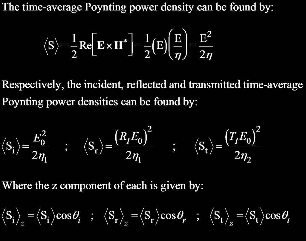
60 Power Conservation 4-6

61 Power Conservation 4-61 P r P t

62 Eample 1 f i E k k [ ] = 1 MH V 1 m = E = = ω µ ε = ω µ ε = π 1 π = = m π f v µ 1 µ ε ε µ µ = = 1 = ε = 4ε Er E i θ i H i k r H r k t E t H t θ = θ = 3 i r 4-6 k π 4π = ω µ ε = ω µ ε εr = 4 = m 3 3 1

63 Eample 1 Cont. f i E [ ] = 1 MH V 1 m = E = µ 1 µ ε ε µ µ = = 1 = ε = 4ε Er E i θ i H i k r H r k t E t H t 4-63 θ = θ = 3 i r k sinθ = k 1 i sinθ t k1 1 sinθt = sinθi = sin 3 =.6 k θ t 1 = sin

64 Eample 1 Cont. k = k sinθ =.5k = k = k 1 i 1 r t k = k cosθ =.866k = k 1 i 1 r µ 1 µ ε ε µ µ = = 1 = ε = 4ε Er E i θ i H i k r H r k t E t H t θ = θ = 3 i r 4-64 t = - = sin θi = k k k k k k you can check by noting that t = cosθt = 4 1cosθt = 1cos14.5 = k k k k k

65 Eample 1 Cont. R R I I = µ k µ k k k = µ k + µ k k + k 1 t t 1 t.866k 1.94k =.866k k t =.38 µ 1 µ ε ε µ µ = = 1 = ε = 4ε Er E i θ i H i k r H r k t E t H t θ = θ = 3 i r 4-65 T I ( k ) µ k k = = = = µ k + µ k k + k.866k k 1 t t Note: T I = 1+ R.618 = 1+ (-. 38) I

66 Eample 1 Cont. R T I E E E S i = 1 = 1 1 η 1 η η I =.38 =.618 µ 1 µ ε ε µ µ = = 1 = ε = 4ε Er E i θ i H i k r H r k t E t H t θ = θ = 3 i r 4-66 E E E E S r = RI = RI RI =.1459 η1 η η η S t = E T I = η E E E TI = TI η η η

67 Eample 1 Cont E E E S i = 1 ; S r =.1459 ; St =.7639 η η η E E Si = Si cos θi = 1 cos3 =.866 η η E E Sr = Sr cos θr =.1459 cos3 =.164 η η E E St = St cosθt =.7639 cos = η η

68 Eample 1 Cont E E E S i =.866 ; S r =.164 ; St.7396 = η η η E.164 η ref. E η tran. E.866 inc. η ( see p.99 for ) general proof

69 Eample 1 Cont. Er θ i k r H r k t E t H t 4-69 E i H i

70 Eample 1 Cont. Im 4-7 Re

71 Eample 1 Cont E y total E 1y E y Standing-wave pattern of the E y field

72 Eample 1 Cont. cosθ =.866 i sinθ =.5 i Er E i k r H r θ i H i k t E t H t 4-7

73 Eample 1 Cont. H total 4-73 H 1 1. η 1 H.54 η Standing-wave pattern of the H field

74 Eample 1 Cont H total H 1.69 η 1 H.31 η Standing-wave pattern of the H field

75 Eample 1 Cont. cosθ ε = 1.94 t r Er θ i k r H r k t E t H t 4-75 E i H i

76 Eample At an Air Seawater boundary, calculate the power density in seawater as compared to that in air for a normally incident wave. air sea water H i E i µ = µ ε = 81 ε µ 1 = µ ε = ε σ mho = 4 m f = 5 [ H]

77 Eample Cont. air H i E i µ 1 = µ ε = ε sea water µ = µ ε σ = 81 ε mho = 4 m f = 5 [ H]

78 Eample Cont. air H i E i µ 1 = µ ε = ε sea water µ = µ ε σ = 81 ε mho = 4 m f = 5 [ H]

79 Direction of Surface Currents E r H r k r 4-79 J = S nˆ H = θ J = (- ˆ ) H S = E i H i E J = ˆ S (- ) η ( k θ) ˆ cos cos cos θ e jk sinθ = o J S = y ˆ E η k cosθ e jk sinθ produces currents only in direction ŷ H E y wire grid

80 Wave Incident on a Good Conductor 4-8 k r k t θ i θ t E

81 Eample 3 ( Prob. 4.1) f = 3 [ MH] parallel polaried µ 1 µ ε ε = µ 1 = ε = ε H r E t E r k r k t θ t H t 4-81 E i θ H i θi = θr = 45 θ = 3 t

82 Eample 3 Cont. E E i i H = ( ˆ k1cosθi ˆ k1sin θi) e ωε = H η ( ˆ ˆ ) e ( ) 1 jk ( + ) jk ( sinθ + kcos θ ) 1 i 1 µ µ Prob ε = µ 1 = ε ε = ε H r E t i E r E i H i θ k r k t θ t θi = θr = 45 θ = 3 t H t 4-8 E r [ ˆ ˆ II jk ( cos ) sin ) 1 θ k k i θ θ 1 ] e = 1 i 1 i R H ωε 1 ( sin kcos θ ) i E r = H η R II ( ˆ ˆ ) e jk ( )

83 Eample 3 Cont. ( Prob. 4.1) µ 1 µ ε ε = µ 1 = ε = ε H r E t E r k r k t θ t H t 4-83 E i θ H i E t T H = ( ˆ k k k sin ) e ˆ II 1 θi ωε 1 θi jk ( sin + k k ) θ = θ = 45 i r θ = 3 t E t.536 = ( 3 ˆ ˆ ) H η e jk ( )

84 Eample 3 Cont. ( Prob. 4.1) 4-84 E H η π k - π k

85 Eample 3 Cont. 1 1 S = Re E H = ηh η1 S i = H 1 = ( Prob. 4.1) R =.718 T = II ; II µ 1 µ ε ε η η H 1 H 1 = µ 1 = ε = ε H r E t E r E i H i θ k r k t θ t θi = θr = 45 θ = 3 t H t 4-85 η1 η η η S r = ( HRII ) = H RII H RII = H.5 TII η TII η H H H η η S t = ( HTII ) = =.813

86 Eample 3 Cont. ( Prob. 4.1) 4-86 η Si 1 ; S r.5 ; St.813 H η H η H = = = S i = η η Si cos θi = H 1 cos45 = H.771 η η Sr = Sr cos θr = H.5 cos 45 = H.36 η η St = St cosθt = H.813 cos3 = H. 735

87 Eample 3 Cont. ( Prob. 4.1) 4-87 η η η Si = H.771 ; Sr H. 36 ; St H.735 = = η H η + H η H.36 ref..735 tran..771 inc.

88 ECE Chapter 4 Reflection and Transmission of Waves 4-88

Reflection/Refraction

$Reflection/Refraction$ Reflection/Refraction Page Reflection/Refraction Boundary Conditions Interfaces between different media imposed special boundary conditions on Maxwell s equations. It is important to understand what restrictions