Ground Motion Prediction Equations in the San Jacinto Fault Zone. Significant Effects of Rupture Directivity and Fault Zone Amplification

Transcription

1 Ground Motion Prediction Equations in the San Jacinto Fault Zone Significant Effects of Rupture Directivity and Fault Zone Amplification I. Kurzon 1, F.L.Vernon 1, Y. Ben-Zion 2 and G. Atkinson 3 1 University of California San Diego, La Jolla, CA, United States. 2 University of Southern California, Los Angeles, CA, United States. 3 University of Western Ontario, London, Ontario, Canada. Submitted to Pure Appl. Geophys. June, 2013 Keywords: Local GMPEs, San Jacinto fault zone, directivity effects, fault zone amplification, regression analysis, engineering seismology 1

2 Abstract We present a new set of Ground Motion Prediction Equations (GMPE s) for horizontal Peak Ground Acceleration (PGA), Peak Ground Velocity (PGV) and 5% damped pseudoacceleration spectra (PSA), developed for the San Jacinto Fault Zone (SJFZ) area. Besides the benefit of these equations to the engineering community in Southern California, the results allow us to examine the physics and local properties controlling ground motions in the SJFZ. The analyzed dataset includes ~ 30,000 observations from ~ 800 events spanning a magnitude range of 1.5 < M < 6.0 and recorded by up to 140 stations at epicentral distances ranging from essentially zero to 150km. The local GMPE is developed for the SJFZ by applying classical regression techniques with predictive variables that include first distance and magnitude, and then site characteristics, rupture directivity, and fault zone amplification. The significance of these effects is determined by measuring the uncertainty-reduction of the GMPE due to each factor. The results show that, in contrast to many regional studies, site characteristic has a relatively minor effect on peak amplitudes in our study area. However, rupture directivity is a significant factor controlling the amplitudes of ground motion even for small events. The dense seismic network and newly developed directivity tool enable us to extract efficiently directivity effects and with statistical significance from the ground-motion dataset during the regression analysis process. The obtained rupture directivities are consistent with the main focal mechanism orientations and surface trace orientations, known from other studies, and predictions for bimaterial ruptures in the trifurcation area of the SJFZ. Fault Zone amplification is a second important factor, showing strong impact on the peak 2

3 ground motion values, with increasing role for the lower frequency range examined in the 5% damped PSA values. We also observe signatures of large amplitude-variances, which indicate additional source-related control on the distribution of amplitudes (besides rupture directivity) for aftershocks close in time and location to the M L 5.1 of March 2013 earthquake. Using the full set of records we present the most complete set of GMPE s for the SJFZ area, including a higher-amplitude prediction for regions in the direction of rupture. 1. Introduction Ground Motion Prediction Equations (GMPE s) provide a fundamental tool for analysis of seismic hazard, by describing the amplitude and attenuation of peak ground motion values from the events to the recording stations. These equations are typically developed by regression of the peak ground motion values to first-order variables such as magnitude and distance, and possibly several other predictive variables. In the past decade there has been extensive work in this field, such as Douglas (2001 and 2003) and the Next Generation Attenuation project (NGA; Abrahamson et al. 2008), in which 5 different groups have developed sets of GMPE s for shallow events in active tectonic regions (Abrahamson and Silva, 2008; Boore and Atkinson, 2008; Campbell and Bozorgnia, 2008; Chiou and Youngs, 2008; Idriss, 2008). These GMPE s were developed on a global or regional scale, combining data from different tectonic settings to enable a larger database to be compiled. However, these large scales tend to generalize and mask some of the local attributes affecting ground motion in specific areas. Moreover, the focus of such GMPEs has tended to be restricted to the upper magnitude range (M>5), 3

4 and they do not always scale well over a broader magnitude range. Recent studies have extended the lower magnitude limit down to M 3 (e.g., Boore et al., 2013; and other GMPEs developed as part of the NGA 2 project) and M 2 (Cua and Heaton 2008), but have retained the global-scale nature of the GMPE s. In this study we develop GMPE s based on data from a single fault system, focusing on a complex region of the San Jacinto Fault Zone (SJFZ) in southern California. The change from a global or regional scale down to a local scale might reduce the role of some effects (such as tectonic settings) on ground-motion variability, while facilitating the identification of other effects not seen in larger scales, some of which might be unique to the study area. We use a rich database of ground motions in the SJFZ to examine: a) what are the main factors controlling amplitudes on a local scale, besides magnitude and distance; b) could these factors shed light on some of the unique characteristics of earthquake physics in the study area and properties of the fault zone; c) what are the differences in the variance of local GMPE s in comparison to that for regional or global GMPE s; and d) what information could we gather on the fault zone and the source from comparing the variance and/or residuals of the GMPE s from different datasets within the same local fault zone (for example different aftershock sequences). The SJFZ provides a great natural laboratory for examining some of the above questions for several reasons: a) it is a highly-active seismic fault, producing a significant number of well-recorded small events ranging up to magnitude 4 along with several larger events; b) it is densely covered by several seismic networks with a recent significant increase in stations due to a SJFZ experiment initiated in 2010 (providing also 4

5 abundant recordings within the immediate vicinity of the fault zone); and c) it encompasses a complex system of faults, with relatively large clusters of seismicity not necessarily aligned with the fault traces or converging to distinct surfaces, and with heterogeneous focal mechanisms of events (Hartse et al., 1994; Bailey et al., 2010). In this study we investigate how the complexity and other characteristics of the fault zone and earthquake processes influence recorded ground motions. By analyzing a highfidelity ground-motion dataset we uncover some of the more dominant amplitudecontrolling factors in the region, clarify their statistical signatures in the data, and apply them to generate fault-zone-specific GMPE s for the SJFZ. 2. Geological Settings The SJFZ is a major component of the strike-slip fault system that accommodates the plate boundary motion in Southern California, branching from the San Andreas Fault at Cajon Pass, crossing the Peninsular Ranges Batholith, and terminating in the desert of the Imperial Valley. The SJFZ has had about 24 km of slip since the latest Pliocene to early Pleistocene (Sharp, 1967; Rockwell et al., 1990; Dorsey and Roering, 2006) and estimated slip rates that vary along strike between 8-20 mm/yr (Rockwell, 2003; Kendrick et al., 2002; Fay and Humphreys, 2005; Fialko, 2006). In this study we analyze data from four major segments of the SJFZ (Figure 1) comprising together the central part of the fault: 1) Clark - Anza (CA), 2) Coyote Creek (CC), 3) Buck Ridge (BR), and 4) Hot Springs (HS). The seismicity in the past 30 years (Hutton el al., 2008; Hauksson et al., 2012) along these segments has been clustered in two main regions (Figure 1): the Hot Springs cluster at a depth range of 15-22km, and the trifurcation (TR) cluster at a 5

6 depth range of 7-17km; between these two clusters there is a distinct gap (Figure 1 topright). The Clark Anza and the Coyote Creek segments are known to have sustained moderate to large earthquakes based on historical and paleoseismic data (e.g. Salisbury et al. 2012; Onderdonk et al. 2013, and references therein). 3. Dataset and data processing We analyze ground motions associated with 800 events in the magnitude range of 1.5 M 6 in a 45km x 125km rectangular area around the SJFZ (Figure 1). The event database consists of the seismicity in the region from February 2010 to May 2012, and three moderate earthquakes (M L 5.6 [M W 5.2] June 2005, M L 5.9 [M W 5.4] July 2010 and M L 5.1 [M W 4.7] March 2013) along with their aftershock sequences. The station distribution includes several networks operating in this region (see Table 1) within a 90km x 275km rectangle around the event epicenters, allowing in most cases good focalsphere coverage of the data. The Peak Ground Acceleration (PGA), Peak Ground Velocity (PGV), and 5% damped Pseudo Acceleration Spectra (PSA) datasets are generated using acceleration and velocity waveforms filtered using a 1-30Hz 4 th order band-pass Butterworth filter (with 4 poles at each corner frequency). The PGA values are mainly used to reveal the factors controlling ground motions, while the PGV and PSA values provide the complete set of GMPE s required for engineering purposes. The relatively high band pass filter of 1 30 Hz used in this study reflects the high frequency content of the data, especially for events in the M < 3 range. The signals for the M > 3 events were chosen preferentially from the acceleration channels due to clipping of the velocity recordings at some of the close- 6

7 range stations, while the signals for the M < 3 events were preferentially taken from the velocity channels due to their higher sensitivity and ability to capture lower magnitude data. Figure 2 displays the magnitude distance distribution of the recordings and the depth distribution of the events used in the PGA analysis. It is shown in two different colors, representing two different datasets: blue for June 2005 and February 2010 to May 2012, and orange for March These two datasets reflect two phases in the evolution of the GMPE s presented here (see section 4). The first phase was done before the aftershock sequence of March 2013, generating GMPE s for 650 events and 20,000 Peak Ground Motion records. In the second phase the March 2013 dataset was merged (addition of 150 events and 15,000 records), providing a new set of GMPE s. There are two main reasons for keeping the results in these two separated phases: a) there are some insights that were observed within the Phase 1 dataset, which were masked by the Phase 2 complete dataset, and b) it demonstrates better the limitations of GMPE s in predicting future motions. These issues are further discussed later in the paper. Note that for the purpose of the GMPE s we use the ML magnitude. Peak values of ground motion were picked automatically using a signal to noise ratio (SNR) algorithm that was tuned to capture the main signal and peak value in each waveform. The tuning was done manually by viewing a significant subset (~ 40%, ~ 2500 records) of the actual peak values of the June 2005 and July 2010 aftershock sequences. A total of 35,000 peak ground records were collected for each one of the datasets (PGA, PGV and for each period of the PSA), from a total of ~ 200 instruments at ~ 140 stations (some stations have a seismometer and an accelerometer). 7

8 4. Data Analysis Procedure We present two different sets of GMPE s, the first set (Phase 1) was generated based on the dataset of June 2005 and February 2010 to May The second set of GMPE s (Phase 2) is based on the merging of the M L 5.1 March 2013 aftershock sequence, which shows very different characteristics from what was predicted by the Phase 1 - GMPE s, and emphasizes additional aspects in the generation of GMPE s. Phase 1 June February 2010 to May 2012 We divide our search for the GMPE s and the factors controlling ground motion values in the SJFZ into several stages. First we consider the two most dominant factors, magnitude and distance, and solve for them using the basic formulation provided by Boore and Atkinson (2008): ( ) + e 3 ( M M h ) 2 + Ln(Y 1 ) = e 1 + e 2 M M h [ c 1 + c 2 ( M M ref )] Ln R 2 2 e + h A [ R ref ] + c 3 R 2 e + h 2 A R ref [ ]. (1) Here M is the local magnitude, R e is the epicentral distance, e 1, e 2, e 3, c 1, c 2, c 3 and h A are regression coefficients, and M h, M ref and R ref are constants. M h, M ref and R ref can be chosen largely for convenience, as long as they are within the range of magnitude and distance of the data (see Boore and Atkinson 2008, for further discussion on this issue). We set M h = 2.5km, R ref = 1km and M ref = 3km. The variable Y 1 gives predicted values based on equation (1) referred to in this study as the basic regression or basic GMPE. We can use the hypocentral distance and regress only for six coefficients, or use the epicentral distance and regress for an additional coefficient, the apparent depth h A. The difference between the two options is minor, but the latter is somewhat advantageous as it 8

9 avoids the addition of depth uncertainties into the total uncertainty, resulting in slightly a smaller uncertainty (~ 0.5%). By using the epicentral distances, h A can be estimated from the maximum amplitude as the epicentral distance approaches zero; deeper apparent depths indicate smaller amplitudes. This is the option chosen in equation (1), where e 1, e 2 and e 3 are magnitude related, c 1, c 2 and c 3, are distance related and h A is the apparent depth of all records. In the second stage we examine additional factors that may affect ground motion peak values using a combination of two main tools. Plotting the observed records together with the basic GMPE, color-coded according to a tentative additional factor, provides a first estimation of the relevance of the examined factor. To quantify that factor we also apply the method used by Thompson et al. (2011) to estimate site response: Ln(Y 2 ) = b 1 + b 2 Ln(X) + b 3 Ln(Y 1 ), (2) where the right side has a linear relation between the examined new factor X, the basic GMPE value Y 1 and the new predicted values Y 2. This equation is an indication of the linearity of Ln(X) with respect to the new GMPE Y 2. Note that when b 3 1 equation (2) approaches a linear relation between the magnitude and distance factors and the additional examined factor. Both equations (1) and (2) provide measures of uncertainties. We use the variance of the models in relation to the observed values, and examine the variance reduction associated with different factors. This allows us to sort different factors according to their relevance and improvements of the GMPE s. Having a current best performing GMPE with the lowest variance, we use the residuals defined as Y observed / Y predicted to search for additional event or station factors that may reduce the variance further. Using the same 9

10 factor-hierarchy we then determine GMPE s for the set of PGV and PSA values, resulting in our estimated GMPE s for the SJFZ area. In the following sections we provide additional details on the main methods used in the data analysis. 4.1 Regression Method Joyner and Boore (1993) introduced two methods for applying regression analysis for finding GMPE coefficients: the one-stage maximum-likelihood method and the two-stage method. In the one-stage method the different uncertainties of the records and events are calculated in one step with a combined uncertainty. In the two-stage method a random record-uncertainty is first calculated, mainly accounting for the event-station distance, and then the event uncertainty is iterated considering the magnitude of each event. Both methods have shown similar success (Joyner and Boore, 1993) and in many of the GMPE studies one of these methods was used as the basic approach (e.g., Boore and Atkinson, 2008). In this work we use the one-stage method to solve equations (1) and (2). The iteration scheme utilizes the golden section search (e.g., Press et al., 1992), allowing a fast convergence to the set of coefficients defining the GMPE s. 4.2 Directivity Method Rupture directivities can produce significant variations of ground motion parameters, with higher frequencies and amplitudes in the direction of rupture propagation compared to the orthogonal and opposite directions (e.g. Douglas et al., 1988; Spudich and Chiou, 2008; Calderoni et al., 2013; Baker et al., 2012, and reference therein, as part of the NGA-West 2 project models). To quantify the effect of rupture directivities on GMPE, 10

11 we use the observed peak ground motion values corrected for geometrical spreading. This is done by multiplying each peak amplitude value, A, by its corresponding hypocentral distance r: A 1/r A corr = A r. (3) The correction (3) is applied up to a distance of km to avoid Pn and Sn phases that can lead to overweighing distant stations. In order to estimate rupture directivity we use 30 wide slices rotated around 360 in 10 increments. For each slice orientation we calculate the average A corr of the A corr values within the slice and search for the slice orientation with the maximum averaged. Since there are other factors that might affect the amplitudes besides distance and directivity (such as radiation pattern or site characteristics), we consider only slices having at least 3 stations and coefficient of variation below The orientation of the slice with A max corr satisfying these requirements is regarded as the rupture direction. Once this direction has been determined, we divide the domain into 12 slices of 30 and use φ to denote the angles between the center of each slice and the assumed rupture direction, i.e., cos(φ) ranges from 1 for the slice of A max corr to -1 for the opposite direction. Finally, we calculate for each slice A corr A max corr = norm A corr where A norm corr ranges from 1 for A max corr to 0 for slices that do not satisfy the forgoing quality criteria. Figure 3 illustrates the directivity tool using data of the M L 5.9 July 7, 2010 event (Figure 3a) and a July 10, 2010 M L 1.6 aftershock (Figure 3b). The waveforms are normalized to the maximum recorded A corr in the stations without applying corrections for geometrical spreading and slice averaging. A close examination shows that the M L 5.9 event has slightly larger amplitudes to the NNE than to the NW, while the M L 1.6 event 11

12 exhibits higher amplitudes to the SE as well as to the NW. The A norm corr vs. cos(φ) plots suggest (see also Figure 4) an approximately unilateral behavior for the M L 5.9 event (Figure 3c) and close to bilateral behavior for the M L 1.6 event (Figure 3d); we note that all slices excluding cos(φ) = 1 or -1 may have two different A norm corr values for the same cos(φ). In Figures 3e and 3f, A norm corr in each slice is assigned back to the stations within that slice and projected onto the map, according to the event-station azimuth θ. The obtained circular map ranges from -1 to 1 on south north and west east axes. The results show the orientation of the stations in relation to the event located in the center of the map, and the event to stations distances reflecting the values of A norm corr in each slice. The orientations of stations with a radius near 1, on the circumference of the circular map, reflect the rupture directivity defined by the azimuth to the middle of the slice containing the stations. This indicates that the M L 5.9 event ruptured to the NE, while the M L 1.6 event ruptured to the southeast, in agreement with the visual characteristics of the waveforms (Figs. 3a, 3b, 3e 3f). Figure 4 presents schematically four end-member cases that can help in understanding the rupture properties: unilateral (Figure 4a) and bilateral (Figure 4b) ruptures, each with weak and strong directivity signals. The strength of the directivity signal is represented by A norm corr defined by the average of A norm corr on all slices. High values of A norm corr reflect a weak directivity signal, since many of the slices besides the one with A max corr have relatively high, possibly reflecting other factors affecting the amplitudes. Low values of A norm corr reflect a strong directivity signal, since the slice of A max corr dominates over other factors affecting the recorded amplitudes. The value of 12

13 A norm corr is also the measure defining the color code in subsequent related figures, with darker blue indicating stronger directivity signal. We define an index of directivity I Dir based on strength of the directivity signal as: I Dir =10 A norm corr A norm corr. (4) The highest I Dir values per event will be for stations that are in the direction of rupture, with stronger signals having higher I Dir values. Events with strong directivity signals will have a wide range of I Dir values, while events with weak directivity signals will show a narrower range of I Dir values. Below we incorporate the variable I Dir in equation (2) to generate directivity-dependent GMPE s. Before applying this tool for the GMPE analysis we demonstrate its utility by translating I Dir to lengths that are plotted with indication of the azimuth of maximum directivity. This is shown in Figure 5 for the M L 5.9 July 2010 event and its aftershocks, along with seismicity from December 2011 at the Hot Springs cluster. The results show that each region has distinct rupture directions that are mainly sub-parallel and subnormal to surface traces within statistical scatter. The waveform observations of the M L 5.9 July 2010 mainshock (Figure 3) indicate a similar NE directivity as the results in Figure 5 in the trifurcation area. We note that a statistical preference of earthquake propagation to the NE in this area is also consistent with observed asymmetry of rock damage (Lewis et al., 2005; Wechsler et al., 2009), combined with theoretical calculations of damage generation during ruptures on a bimaterial fault (Ben-Zion and Shi, 2005; Xu et al., 2012) and recent detailed tomographic images (Allam and Ben-Zion, 2012, Allam et al., 2013). The other Hot Springs cluster of seismicity in Figure 5 is off the main San Jacinto fault and requires additional information to interpret. A more 13

14 detailed analysis of the directivity tool and its possible implications will be given in a follow up paper (Kurzon et al., 2013). 4.3 Obtaining PSA values The response spectra providing the 5% damped Pseudo Spectral Acceleration (PSA) values is calculated using the classical algorithm of Nigam and Jennings (1969) for solving the equation of motion of a simple oscillator: χ + 2βω χ +ω 2 χ = a(t), (5) where t is time, ω is the natural frequency of the oscillator, β is the damping coefficient, and a(t) is the base acceleration the oscillator is subjected to. A segmental linear approximation of a(t) is given by: χ + 2βω χ +ω 2 χ = a i ( t t i ) ( a i+1 a i ) ( t i+1 t i ) t i t t i+1. (6) Since χ and χ are known at t = 0, one can solve (6) analytically and obtain displacement, velocity and acceleration for each examined ω (Nigam and Jennings, 1969), which in this study spans a frequency range of Hz. Phase 2 Merging the M L 5.1 March 2013 aftershock sequence The M L 5.1 March 2013 aftershock sequence was recorded on the complete network of the SJFZ project, providing many more stations within the fault zone, including two additional linear arrays that did not exist in the Phase 1 dataset; altogether 30 more stations within 1 km distance from fault segments. In Phase 2 dataset there are additional 150 new events and 15,000 new records augmenting the 650 events and 20,000 records of 14

15 the Phase 1 dataset. Naturally, this has changed some of the balances within the merged dataset, and with a combination of a very different source behavior (discussed later in the text) we had to modify our approach. The actual method applied in Phase 2 is described in Section 6 Results Phase 2 5. Results Phase 1 We first examine the PGA dataset and by a combination of regression and residual analysis obtain a best-fit basic GMPE for PGA values. We then use the factor hierarchy found during the process of the PGA analysis to develop a complete set of GMPE s for the PGV and PSA values. 5.1 Stage 1 PGA Analysis Basic Regression for magnitude and distance Figure 6 shows results of the basic regression in four magnitude bins, obtained by solving Equation (1) with the one stage algorithm of Joyner and Boore (1993), along with an uncertainty measurement of σ t = The uncertainty is quantified by the standard deviation values σ t, σ e and σ r, where σ t is the total uncertainty of all records given by the sum of variability within the events σ e and random variability of the records σ r. The value σ t = is our basic uncertainty that serves as a reference for analysis of additional factors made in the following regression steps. Figure 6 and Table 2 compare our results with GMPE s generated for other datasets in regions around our study area: Boore et al. (2013) denoted BSSA13 and Cua and Heaton (2008) denoted CH08. The results of BSSA13 were developed for western US 15

16 over a magnitude range of 3 M 8. The results of CH08 are for Southern California over a magnitude range of 2 M 7.3, and have two solutions depending on V s30 value of site characteristics corresponding to soil and rocks, where V s30 denotes the average shear wave velocity in the top 30m of the crust. The amount of events and records examined in our work, BSSA13 and CH08 are different, with total number of records increasing from CH08 to BSSA13 to our work (Table 1). In addition, our analysis includes higher frequencies than the traditional 1 10Hz band. These differences should be considered when comparing the results Factor Analysis We consider three effects that can be significant for recorded ground motion in the SJFZ area. The first is site characteristics, mainly measured by V s30, reflecting the soil conditions at the recording station. The second is fault zone amplification not captured by V s30, reflecting path effects involving rock damage in a region around the fault. The third is the rupture directivity, exhibiting higher amplitudes for stations in the direction of rupture. The analysis is done by applying Equation 2 for each of the above factors, as well as color-coding the records for each factor and looking for a clear color-signature. Site Characteristics The classical characterization of site conditions is done via V s30, with higher values corresponding to rock sites and lower ones related to soil (or highly weathered rock) sites. There are many ways of quantifying V s30, either by measurements, or by spatial estimations, as geological or topographical. For the stations in our study there are only a 16

17 handful of actual V s30 measurements, so we test the following geological and topographical V s30 estimations of the region. 1) Geological estimation according to Wills et al., 2000, (W00), 2) Geological estimation according to Wills and Clahan, 2006, (WC06), 3) Topographical slope estimation according to Wald and Allen, 2007, (WA07) using a) SRTM30 (Shuttle Radar Topography Mission) with 30 arc-sec resolution and b) SRTM3 with 3 arc-sec resolution, and 4) a statistical compilation of measurements and estimations in Southern California (Yong et al., 2012). Our analysis indicates that neither of these estimations has a significant affect on the recorded amplitudes in our SJFZ data set. Figure 7 shows results for estimates based on SRTM30 and Yong et al. (2012). The SRTM30 estimation does not produce a clear observable signal (Figure 7a). The Yong et al. (2012) V s30 estimation has a weak observable signal, indicating as expected that rock sites tend to have higher amplitudes than soil sites (Figure 7b). This signal is seen for the magnitude range of 2 M 4 and is probably masked in the lower range by scattering effects. Applying Equation 2 and regressing for both estimates, we find (Table 3) that the uncertainty reduction in both cases is very small: 0.01% for the SRTM30 and under 0.2% for the Yong et al. (2012) estimation. This is perhaps not very surprising, given that many of the sites are on rocks in an arid and mountainous terrain, where soil development is relatively poor. Fault Zone amplification Our use of a very dense network of stations around the SJFZ (Figure 1) allows us to test for statistical changes in the ground motion amplitudes related to distance from the fault. Starting with the initial deployment of the NSF SJFZ CD project in September 17

18 2010, there has been a progressive significant increase in the number and density of nearfault stations. We therefore do not expect a clear effect prior to that time; specifically the two M L > 5 events in our database are not expected to show this effect. Indeed, Figure 8 shows a clear signature of fault zone amplification in the 2 M 4 range but not in higher magnitudes. The lower range M < 2 might suffer from scattering effects, namely the higher involved frequencies may be masked by scattering which is typically in the same high frequency band. Table 3 shows that fault zone amplification is overall more effective than what was found for the V s30 estimates with an uncertainty reduction of 1%. Rupture Directivity We implement the directivity tool of section 4 within the regression algorithm, assigning index of directivity I Dir for each PGA record corresponding to each station orientation in each event. The color-coded values of I Dir show (Figure 9) a clear signature in the complete range of magnitudes for many of the records satisfying the statistical requirements stated in section 4. Table 3 indicates that the directivity index has the most significant effect among the three examined factors, producing a 7.4% uncertainty reduction. Hierarchical ordering of factors To separate and quantify different factors, we regress each factor in hierarchical order based on their separate significance. Since the site characteristic signature is very small we neglect it and perform sequential regressions first for directivity and then for fault zone amplification. 18

19 5.1.3 The Addition of Directivity to the GMPE Figure 10 displays the original records, along with the basic GMPE and the values calculated by GMPE Dir, providing the new GMPE including the directivity factor. Since for each record we assign an index of directivity, we obtain the same number of points as the original records with vertical spread reflecting how well they cover the original data. The wider the spread of the GMPE Dir results around the basic GMPE, the better they explain the data with a higher variance reduction. As seen, the directivity can explain in our case almost an order of magnitude of the two orders of variability in the dataset, leaving the remaining variability to be explained by other factors Residual Analysis To clarify effects of additional factors affecting the PGA values we perform a residual analysis. We define residuals as the ratio between the observed PGA and values provided by the GMPE Dir : res = PGA / GMPE Dir, and examine the residuals per station in the same magnitude bins as in the previous sections. Figure 11 shows the residuals per station, with a color scale ranging from blue, through green and orange, to red for increasing residuals, which are also scaled by the increasing size of the circles. In each magnitude bin we identify three classes of stations: 1) those showing the whole range of residuals, 2) stations dominated by low residuals, and 3) stations dominated by large residuals. To simplify the pattern we display in Figure 12 stations based on the 3 ranges of minimum and maximum residuals (res min and res max ): 1) stations with res min 0.5 and res max 2 designated as amplifiers and marked in red, 2) stations with res min 0.5 and 19

20 res max 2 designated as dampers and marked in blue, and 3) all the rest considered as good-fit and marked in green. In the magnitude range 1.5 M 4 there are stations showing a clear tendency for being amplifiers, dampers, or good-fit (Figure 12). The M > 5 bin has the smallest amount of data and probably largest statistical fluctuations reflecting detailed factors of individual events not examined here. To highlight the general tendencies of stations, we calculate an average,, where i covers the 3 magnitude bins in the range 1.5 M 4 where we have ample data. Figure 13 shows three station categories based on this calculation: amplifiers with Avg 2/3 (red), dampers with Avg 1/3 (blue) and good-fit with 1/3 < Avg < 2/3 (green). Examination of the amplifiers and dampers reveals two clear effects. One involves 8 dampers associated with boreholes or postholes stations in a depth range of m. This may be since these stations are located below the low shear-velocity surface layer (~ 5-10m depth, e.g., Louie, 2001; Wu and Huang, 2013), in which the benefit of removing high-frequency surface noise is bundled with the drawback of loosing some of the high amplitudes of high-frequency seismic signals, resulting in some cases with lower amplitudes (Al-Shukri et al., 1995; Vernon et al., 1998). The second category involves surface stations that are within 3km normal-to-fault distances including the three linear arrays crossing the Anza/Clark segment. Almost all stations within that distance are amplifiers and reflect probably reduced elastic moduli associated with damaged fault zone rocks (e.g., Ben-Zion and Sammis, 2003, and references therein). These two effects can be treated separately in the process of improving the GMPE, by assigning the following station indices: 100 for amplifiers, 0.1 for dampers and 1 for the rest. Using these station values in the regression process according to Equation 2 leads to: 20

21 Ln(Y 3 ) = b 11 + b 12 Ln(X) + b 13 Ln(Y 2 ), (7) where Y 2 = GMPE Dir, X is the vector of the assigned indices and Y 3 is the resulting GMPE. Figure 14 presents the results where the original PGA values are plotted together with the basic and new GMPE, GMPE Dir+FZBH, accounting for the directivity effect, the Borehole damping (BH) and Fault Zone amplification (FZ). The color code corresponds to the amplifiers, dampers and good-fit stations. The uncertainty is reduced (Table 3) from σ t = for the GMPE Dir solution to σ t = for this new solution GMPE Dir+FZBH, reflecting additional uncertainty reduction of 4.9% and a total reduction of 11.9% relative to the basic GMPE. This is the final result based on the uncorrected database used in our first stage analysis. 5.2 Stage 2 PGV and 5% Damped PSA Analysis The procedure used for the PGA analysis has the following steps: 1) regression for magnitude and distance, 2) regression for rupture directivity, 3) residual analysis for GMPE Dir and identification of amplifiers and dampers, and 4) additional regression for borehole damping and fault zone amplification. Applying the same procedure to the PGV and PSA datasets we obtain a full set of GMPE s presented in Tables 4-6. The different GMPE s presented in these tables have several interesting features outlined below. The Apparent Depth As mentioned, the apparent depth h A reflects the mean depth estimated by the regression. The deeper the value of h A the lower the amplitudes in the close epicentral distances The longer periods of the PSA equations have significantly lower h A values 21

22 than the one of the PGA, indicating that the lower frequency range is amplified in comparison to the PGA equation. This is consistent with basic spectral decay properties. σ t of the Basic Regression The uncertainty of the basic regression also shows that the longer periods of the PSA range is noisier, having larger σ t values. A plausible reason is that the PGA values are dominated by the shorter period range of the spectra, so the PSA values generated by Equation (6) for the short periods represent the dominant frequencies determining the PGA values. The longer periods are not the dominant spectral band, therefore generating a larger scatter of PSA values with corresponding larger σ t values. δσ t of GMPE Dir and GMPE Dir+BHFZ The uncertainty reduction due the addition of directivity, borehole damping and fault zone amplification reveals an interesting effect. The PGA and shorter period PSA show high δσ t in relation to the directivity (Table 5) and lower δσ t in relation to the borehole damping and fault zone amplification (Table 6). For longer periods the tendency flips, with lower values of δσ t in relation to directivity than in relation to BHFZ. This may be explained partially by the fact that the higher frequency range works the best for the directivity tool, and the dominance of fault zone amplification for lower frequencies may reflect trapped waves and other phases in fault damage zones (e.g. Ben-Zion and Aki, 1990; Li et al., 1994; Ben-Zion et al., 2003). 6. Results Phase 2 22

23 The aftershock sequence of the M L 5.1 from March 2013 was recorded by a denser network than the previous events, adding ~ 40 stations to the network, with 20 being part of two linear arrays across the San Jacinto Fault. The initial merging of the data failed the basic regression for magnitude and distance (equation (1)) used in the first phase, and required a different approach. Several subsets excluding stations and/or events were attempted and led to large uncertainties (σ t ~ 1.2) when regression succeeded. The initial efforts indicated that there is something different about this new dataset, and that the additional fault zone stations might also contribute to the diversity of results. This suggested that there is an additional factor (or factors) that should be treated as a firstorder factor like magnitude and distance. Both the directivity and fault zone amplification were examined, using a similar equation as equation (1), only with an additional term, d 1 Ln(X), for the contribution of the examined factor. While the fault zone amplification term failed in the regression, the directivity proved very useful, providing new GMPE s with reduced variance for the different subsets examined. The new formulation used for the regression is: ( ) + e 3 ( M M h ) 2 + Ln(Y 1 ) = e 1 + e 2 M M h [ c 1 + c 2 ( M M ref )] Ln R 2 2 e + h A [ R ref ] + c 3 R 2 e + h 2 A R ref [ ] + (8) d 1 Ln I Dir ( ), where d 1 is the coefficient for the directivity term, and generates GMPE Dir solutions as in Phase 1. We can reverse now and replace the last term in equation (8) with d 1 Ln( I Dir ), in which I Dir is the average of the I Dir values, providing a discreet basic GMPE as was generated in the initial stage of phase 1. Figure 15 shows a comparison between two datasets, the one used for Phase 1 (blue), 23

24 and the additional dataset of March 2013 (orange-red). Figure 15a presents the PGA records together with their corresponding basic GMPE s generated by equation (8), replacing the last term by d 1 Ln( I Dir ), and Figure 15b shows the basic GMPE s together with their corresponding GMPE Dir. Although the spread of PGA values is overlapping for both datasets, there is a larger variance for the March 2013 dataset, seen in the lower magnitude range, especially 1.5 M 2. The basic GMPE for March 2013 shows higher-amplitude attenuation curve than the ones produced for the Phase 1 dataset, especially in the closer epicentral distance Re < 10km. The GMPE Dir seen in Figure 15b accounts for magnitude, distance and rupture directivity, explaining a significant proportion of the variance of the original PGA records: a) for the dataset of March beginning with no conversion when using equation (1), through σ t =1.2 for pre-averaging of the arrays, to σ t =1.044 when using equation (8), and b) for the Phase 1 dataset - from σ t =0.968 when using equation (1) to σ t =0.894 when using equation (8), which is similar to the σ t =0.896 of the Phase 1 - GMPE Dir (see Table 7). Merging the March 2013 with the Phase 1 dataset, we have taken one more measure to improve our GMPE s, setting epicentral distances cutoff for different ranges of magnitudes. We have set the epicentral distances for the new merged dataset (Phase 2) to be M < 3 up to 80km, 3 M < 5 up to 100km, and 5 M < 6 up to 150km (Figure 16a). These settings decrease the weight of small events in large distances, allowing the larger distances to be dominated by the larger events, and reducing some of the noise affecting the generation of the GMPE s. Figure 16b shows a comparison between several different GMPE s for the PGA records of Phase 2, in relation to the Phase 1 - basic GMPE represented by a dashed black line. The GMPE Dir spread (blue color scale) is similar to 24

25 what was seen in phase 1 with a σ t =0.92 (slightly higher than the Phase 1 - GMPE Dir solution) and the bold black curve is the basic GMPE derived from replacing the last term in equation (8) with d 1 Ln( I Dir ). We added another solution here, basic GMPE HighDir (blue curve), obtained by considering only the GMPE Dir values larger than I Dir and averaging them. This provides an amplified GMPE that should be applied for sites that are in the direction of rupture. For hazard assessment this kind of prediction might be more meaningful than the basic GMPE, or the GMPE Dir. In fact, it does something similar to the directivity predictive models implemented in GMPE s (e.g., Spudich et al and references therein), providing an upper attenuation curve estimation for regions within the direction of rupture. Calculating the residuals of the Phase 2 - GMPE Dir in relation to the observed PGA records, we examined whether we see special tendencies in station or events distribution. An initially surprising result was that we could not see any similar station distribution, indicating Fault Zone amplification, as we have seen in the Phase 1 residual analysis (Figure 13). This may stem from two possible reasons. First, the new GMPE curves are amplified in relation to the Phase 1 - GMPE s, partly due to the increasing weight of stations and records within the Fault Zone, so that the GMPE already includes (at least partially) fault zone amplification. Second, there is something different in a significant portion of the March 2013 records, providing PGA values with a larger spread per magnitude-distance, so that any Phase 1 tendencies are masked by the new records; this is suggested by the large uncertainty of the March 2013, which hardly changed, even for different subsets of stations (Table 7). Figure 17 presents a residual analysis for the events, where the variance of the 25

26 residuals per event, res var, is plotted; large res var reflects large variance of the residuals and is associated with amplified events, and small res var reflects small variance of the residuals and is associated with damped events. We use a color scale in which 0.5 res var 2 is a reasonable value per event (green), and beyond these limits res var might indicate a spatial or source signature. Since we are interested in explaining some of the difficulties we had regressing the March 2013 dataset and understanding the large uncertainty associated with it, we examine mainly the large res var (orange to red) values. If a group of events are clustered in space and/or time and show a clear tendency in their res var values, this would indicate that something about the source mechanisms or source region is dominating the amplitudes recorded for the event. Figure 17a shows the complete Phase 2 residual analysis in all magnitude bins. The higher range of magnitudes, 3 M < 6, seem to have small res var values, especially the M L 5.1 of March 2013 (blue), so we should examine closer the lower magnitude range of 1.5 M < 3. Figures 17b - 17e compare results for three subsets: 1) the main shocks, which are events with no clear aftershock sequences within the dataset, 2) the June 2005 and July 2010 aftershock sequences, and 3) the March 2013 aftershock sequence. The main shocks in Figure 17b have low to high res var values, in which possible spatial tendencies could be identified, such as the low res var in the SE of the fault, and in two clusters: to the NW of the Trifurcation, and to the SE of the Hot Springs cluster. The June 2005 and July 2010 (Figure 17c) are mainly dominated by mid-range res var values, which are also reflected by the corresponding low value of uncertainty (Table 7). The March 2013 dataset (Figure 17d) displays the entire range of res var, but events in the main cluster in the close vicinity of the M L 5.1 have relatively high values of res var (orange to red). This indicates that the 26

27 main source region and/or mechanisms are dominating the large res var values and the large uncertainty seen for the March 2013 dataset. Even after considering only the stations that existed also in the Phase 1 dataset (Figure 17e), there is still a clear signature of large res var values, which is especially pronounced for the 1.5 M < 2 range. Removing all the new stations out of the March 2013 dataset leads to uncertainty reduction by less than 1% (from σ t = to σ t = 1.035). 7. Discussion The two phases of this research illuminate different aspects of the development of GMPE s in a local system, and what considerations should be taken to account for the main factors controlling ground motions. The first phase emphasized the roles of rupture directivity, fault zone amplification, posthole damping and site characteristics, in determining the amplitude of ground motions. The second phase showed the effects of a) including different source mechanisms and/or source regions, and b) shifting the station balance towards including more stations from the fault zone. Both phases were essential for the insights presented in this paper discussed further below. Removing the Vs30 for the SJFZ One of the interesting outcomes of this study is the insignificant role of site characteristics for GMPE s in the SJFZ, unlike many other studies (e.g., Cua and Heaton, 2008). Although we have shown that site-characteristics have a signature within the data (Figure 7b), this signature did not translate into a significant factor affecting a large proportion of the data. Furthermore, it could be seen that the majority of records were 27

28 classified as rock sites according to Yong et al. (2012), which might explain the small effect the minority of soil sites had on the overall data. This is not surprising since most of the sites of the Anza and SJFZ project stations were installed in granite or weathered granite (Sharp, 1967) that, while being softer, seems to have similar site characteristics as un-weathered granite. For these reasons we have chosen to remove this factor from our analysis, although it should be considered in a study including minor effects. Perhaps for M > 5 events, some of the soil sites and maybe even the weathered granite would show non-linear amplifications as seen in other works (e.g., Boore and Atkinson, 2008). However, for that range we do not have enough data for analysis. Directivity of Rupture Besides the ability of the directivity tool to identify the rupture directivity (Figure 5), we have seen that implementing the tool within the GMPE regression scheme reduces successfully the uncertainty of the peak ground motion values. This notion, derived initially through the Phase 1 analysis, is implemented in Phase 2, allowing the regression to successfully generate the GMPE s (which without this factor was failing to converge). In addition, as seen in the Phase 2 analysis, the directivity factor is significant enough in the SJFZ to be considered as a first-order factor, similar to magnitude and distance. Deriving the basic GMPE HighDir for the direction of rupture (see Figure 16b) provides a possibly more significant attenuation curve for the use of engineers, estimating an upper limit for the expected ground motions. This upper limit, which is higher by a factor of 2 from the Phase 2 basic GMPE, has a similar effect as the directivity models implemented in the NGA-West 2 GMPE s (e.g., Spudich et al., 2012, and references 28

29 therein), estimating the upper shift of the attenuation curves in the direction of rupture. The advantage in our model is that we do not assume anything about the source; the directivity tool reveals the nature of the seismic events directly from the peak ground motion values. This was shown to be effective for M < 5 ; for the small number of highmagnitude events in the dataset, the directivity tool shows weak directivity signals, which might be a result of masking by other factors (such as non-linear site response or a dominant radiation pattern). For M > 5 events, the source-model-based approach (e,g., Spudich and Chiou, 2008) might provide a more reliable estimation for sites in the direction of rupture. The larger uncertainty seen in the basic GMPE HighDir may originate in the fact that the directivity tool is mainly sensitive to the difference between stations in the direction of rupture, as opposed to stations in other directions. It is not as sensitive to the differences in between the records with high directivity signals. Note that for the PGA and PGV we could set even higher levels of I Dir to generate higher curves of basic GMPE HighDir but for consistency reason we used the minimum I Dir possible so that also the PSA records would converge. The persistent directivity observed for the trifurcation area (Figure 5) is consistent with theoretical predictions for bimaterial ruptures with preferred propagation direction (e.g., Andrews and Ben-Zion, 1997; Ben-Zion and Shi, 2005; Ampuero and Ben-Zion, 2008) associated with the local velocity structure (Allam and Ben-Zion, 2012; Allam et al., 2013) and observed asymmetry of rock damage across the SJFZ (Lewis et al., 2005; Wechsler et al., 2009). A more informative comparison between observed directions of earthquake ruptures in different sections of the SJFZ and theoretical predictions for 29

30 bimaterial ruptures is left for future work. Fault Zone Amplification Fault Zone Amplification shows a very dominant role in the Phase 1 analysis. In fact, as noted above, since many of the new stations (the additional ones of March 2013) are located in the fault zone, the weight of fault zone stations contributes to the higher curves of Phase 2 - GMPE s (Figure 16b). Amplification of ground motions in the fault zone could be the outcome of several reasons. 1) Body wave amplification resulting from the radiation pattern of the source with different orientations for the P and S phases (e.g., Aki and Richards, 2002). 2) Trapped waves and other internal reflections within the damage zone (e.g., Ben-Zion and Aki, 1990; Li et al., 1994; Ben-Zion et al., 2003). 3) Reduction in stiffness within the damage zone might cause amplification on the normal component close to the fault (e.g., Pischiutta et al., 2012, 2013). 4) Rupture directivity, discussed above, is in most cases parallel or sub-parallel to the fault zone orientation (when slip surfaces are also parallel to the fault zone orientation), leading to amplification in the direction of rupture for nearfault stations. The specific factors or combination of factors for fault zone amplification in the SJFZ could be revealed by a careful examination of the normal parallel and radial transversal coordinate systems, under different frequency bands. For example, the directivity tool could be set in different levels of confidence, using the radial transversal vertical coordinate system, and analyzing separately the P and S phases. Such detailed analysis may be done in a follow up work. From the Phase 1 analysis of the PGA and PSA values we observe (Tables 5, 6) an 30

31 interesting trend. The PGA and shorter period PSA values are more affected by the directivity factor than by the fault zone amplification and borehole-damping factor. However, for longer period PSA values the trend reverses showing stronger effects of the fault zone amplification. This provides an estimation of the frequency bands where these effects are dominating, and reflects the lower frequency phases characterizing the fault zone, together with the shift to higher frequencies in the direction of rupture (e.g., Douglas et al. 1988). The Phase 2 - GMPE s for the PSA values support the above insights, showing that the directivity effect is more dominant in the shorter periods than in the longer ones (Tables 8,9). However, the levels of uncertainty are significantly larger than the PGA. The larger uncertainties may reflect a) the larger variation seen in the source region of the March 2013 (Figure 17), and b) the higher weight of fault zone stations, introducing more noise into the directivity signals even at high frequencies (possibly more scattering). 8. Conclusions We have developed two sets of GMPE s for horizontal peak ground motions, for PGA, PGV and 5% damped PSA records, appropriate for the SJFZ. These equations account for magnitude, distance, rupture directivity, fault zone amplification and borehole damping. We have shown that besides the obvious distance and magnitude factors, rupture directivity and fault zone amplification have a significant role in explaining some of the variation seen in the observations. According to the Phase 1 analysis, the overall uncertainty reduction due to both factors ranges from 12 17%, for the PGA and PSA values. In the Phase 2 analysis the fault zone amplification seems to 31

32 shift up the peak ground motion values, showing higher GMPE curves, and rupture directivity explains a significant amount of the data-variation. In Phase 1, there is a shift in the impact of directivity and fault zone amplification, from a more dominant directivity effect, for the PGA and high frequencies PSA, to a more dominant fault zone amplification and borehole damping for the lower frequency range of the PSA (longer periods). A similar tendency is seen in the Phase 2 dataset, in which directivity shows smaller uncertainties for the PGA and short period PSA GMPE s. The directivity tool has been found to be a powerful method, not only for the generation of GMPE s, but also for a closer study of the fault segments and their tendency to rupture in specific directions. Fault zone amplification seem to also play an important role in affecting the peak ground motion, and further work should be done to identify the specific sources of this effect. The roles of both factors is significantly more important in the examined data than the traditional consideration of site characteristics, maybe due to the fact that many of the sites, even in soft ground, should be considered as rock site. The Phase 1 GMPE s, although illuminating nicely the main factors controlling ground motions, is incomplete. We believe that the more statistically robust Phase 2 - GMPE Dir is the most representative of the region, accounting for larger variability in station location, and source mechanisms, and providing a better prediction for the sites in the close field of the events. In fact, by masking fault zone amplification due to the large weight of fault zone stations, the Phase 2 - GMPE Dir reflects the narrow band around the fault segments (~1km wide). The Phase 2 basic GMPE HighDir provides even a higher estimation for sites in the direction of rupture, and should also be considered. Currently 32

33 there are no data that would allow us to extend the analysis of ground motion parameters in the SJFZ environment for larger earthquakes (M>6), which is a significant practical limitation of the present study. However, such events are expected to occur in the nottoo-distant future (Zoeller and Ben-Zion, 2013; Working Group on California Earthquake Probabilities < and could be used to test the generality and extent of our results. The large difference seen in the GMPE s from Phase 1 to Phase 2, should serve as a cautionary note in using GMPE s to predict future motions, comparing different datasets, and applying models to new datasets. It is not necessarily true that in a specific region, a model developed for that region would do a better prediction than a model developed for another dataset and region. Data Sources Seismic data used in this study are gathered and managed by the following networks: 1. The Anza network (AZ) and the SJFZ (YN) network are operated by IGPP, University of California, San Diego < 2. The SCSN network (CI) is the Southern California Seismic Network operated by Caltech and USGS < 3. The PBO network (PB) is the Plate Boundary Observatory operated by UNAVCO < 4. The SB network is operated by University of California, Santa Barbara < 33

34 5. Gaps in data were filled by the IRIS Data Management Center (DMC) < 6. Instrumentation for seismic stations was provided by IRIS PASSCAL < Grids for maps were downloaded from the web-tool: < Acknowledgements Ittai Kurzon thanks Luciana Astiz for her kind guidance and for suggestions on the first draft of this paper, and also Alan Yong from the USGS for the Vs30 estimations per site presented in this paper. The study was supported by the National Science Foundation (grant EAR ) and Ittai Kurzon was partly supported by a post-doctoral fellowship from the Geological Survey of Israel. Bibliography Abrahamson, N. A., G. M. Atkinson, D. M. Boore, Y. Bozorgnia, K. W. Campbell, B. Chiou, I. M. Idriss, W. J. Silva, and R. R. Youngs (2008). Comparisons of the NGA Ground-Motion Relations, Earthquake Spectra, 24(1), Abrahamson, N. A. and W. J. Silva (2008). Summary of the Abrahamson and Silva NGA Ground-Motion Relations, Earthquake Spectra, 24(1), Aki, K., & P. G. Richards (2002). Quantitative Seismology (second edition), University Science Books. 34

35 Allam, A. A. and Y. Ben-Zion (2012). Seismic Velocity Structures in the Southern California Plate-Boundary Environment from Double-Difference Tomography, Geophys. J. Int., 190, , doi: /j X x. Allam, A. A., Y. Ben-Zion, I. Kurzon and F. L. Vernon (2013). Seismic velocity structure in the Hemet Stepover and Trifurcation Areas of the San Jacinto Fault Zone from double-difference tomography, Bull. Seism. Soc. Am., in review. Al-Shukri, H. J., G. L. Pavlis and F. L. Vernon (1995). Site Effects Observations from Broadband Arrays, Bull. Seismol. Soc. Am., 85(6), Andrews, D. J. and Y. Ben-Zion (1997). Wrinkle-like Slip Pulse on a Fault Between Different Materials, J. Geophys. Res., 102, Ampuero, J.-P. and Y. Ben-Zion (2008). Cracks, pulses and macroscopic asymmetry of dynamic rupture on a bimaterial interface with velocity-weakening friction, Geophys. J. Int., 173, , doi: /j X x. Bailey, I. W., Y. Ben-Zion, T. W. Becker, and M. Holschneider (2010). Quantifying Focal Mechanism Heterogeneity for Fault Zones in Central and Southern California, Geophys. J. Int., 183, Baker, J. W., Y. Bozorgnia, C. Di Alessandro, B. Chiou, M. Erdik, P. Somerbille, and W. Silva (2012) GEM-PEER Global GMPEs project Guidance for including Near-Fault Effects in Ground Motion Prediction Models, Proceedings of 15 th World Conference on Earthquake Engineering, Lisbon, Portugal, 10p. Ben-Zion, Y. and Shi, Z. (2005). Dynamic Rupture on a Material Interface with Spontaneous Generation of Plastic Strain in the Bulk, Earth Planet. Sci. Lett., 236, , DOI: /j.epsl

36 Ben-Zion, Y. and K. Aki (1990). Seismic radiation from an SH line source in a laterally heterogeneous planar fault zone, Bull. Seism. Soc. Am., 80, Ben-Zion, Y. and C. G. Sammis (2003). Characterization of Fault Zones, Pure Appl. Geophys., 160, Ben-Zion, Y., Z. Peng, D. Okaya, L. Seeber, J. G. Armbruster, N. Ozer, A. J. Michael, S. Baris and M. Aktar (2003). Shallow fault zone structure illuminated by trapped waves in the Karadere-Duzce branch of the North Anatolian Fault, western Turkey, Geophys. J. Int.,152, Ben-Zion, Y. and Z. Shi (2005). Dynamic rupture on a material interface with spontaneous generation of plastic strain in the bulk, Earth Planet. Sci. Lett., 236, Blisniuk, K., T. Rockwell, L. A. Owen, M. Oskin, C. Lippincott, M. W. Caffee, and J. Dortch (2010). Late Quaternary Slip Rate Gradient defined using High-Resolution Topography and 10Be Dating of Offset Landforms on the Southern San Jacinto Fault Zone, California, J. Geophys. Res., 115, B08401, doi: /2009JB Boore, D. M., and G. M. Atkinson (2008). Ground Motion Prediction Equations for the Average Component of PGA, PGV, and 5%-damped PSA at Spectral Periods between 0.01s and 10.0s, Earthquake Spectra, 24(1), Boore, D. M., J. P. Stewart, E. Seyhan, and G. M. Atkinson (2013). NGA-West 2 Equations for Predicting Response Spectral Accelerations for Shallow Crustal Earthquakes, PEER Report 2013/xx, Pacific Earthquake Engineering Research Center, Berkeley, California. 36

37 Calderoni, G., A. Rovelli, and S. K. Singh (2013). Stress drop and source scaling of the 2009 April L Aquila earthquakes, Geophys. J. Int. (2013) 192, Campbell, K. W. and Y. Bozorgnia (2008). NGA Ground Motion Model for the Geometric Mean Horizontal Component of PGA, PGV, PGD and 5% Damped Linear Elastic Response Spectra for Periods Ranging from 0.01 to 10 s, Earthquake Spectra, 24(1), Chiou, B. S. J. and R. R. Youngs (2008). An NGA Model for the Average Horizontal Component of Peak Ground Motion and Response Spectra, Earthquake Spectra, 24(1), Cua, G. and Heaton, T. H. (2008). Characterizing Average Properties of Southern California Ground Motion Amplitudes and Envelopes, Bull. Seismol. Soc. Am., submitted. Douglas, A., J. A. Hudson and R. G. Pearce (1988). Directivity and the Doppler effect, Bull. Seismol. Soc. Am., 78(3), Douglas, J., (2001). A Critical Reappraisal of Some Problems in Engineering Seismology. PhD thesis, University of London. Douglas, J., (2003). Earthquake Ground Motion Estimation Using Strong-Motion Records: a Review of Equations for the Estimation of Peak Ground Acceleration and Response Spectral Ordinates, Earth-Science Reviews, 61, Dorsey, R. J. and J. J. Roering (2006). Quaternary Landscape Evolution in the San Jacinto Fault Zone, Peninsular Ranges of Southern California: Transient Response to Strike-Slip Fault Initiation, Geomorphology, 73,

38 Fay, N., and G. Humphreys (2005). Fault Slip Rates, Effects of Elastic Heterogeneity on Geodetic Data, and the Strength of the Lower Crust in the Salton Trough region, Southern California, J. Geophys. Res., 110, B09401, doi: /2004jb Fialko, Y. (2006). Interseismic Strain Accumulation and the Earthquake Potential on the Southern San Andreas Fault System, Nature, 441, doi: /nature04797, Hartse, H. E., M. Fehler, R. C. Aster, J. S. Scott and F. L. Vernon (1994). Small-scale heterogeneity in the anza seismic gap, southern California, J. Geophys. Res., 99(B4), Hauksson, E., W. Yang and P. Shearer (2012). Waveform Relocated Earthquake Catalog for Southern California (1981 to June 2011), Bull. Seismol. Soc. Am., 102(5), Hutton, K., J. Woessner and E. Hauksson (2008). Earthquake Monitoring in Southern California for Seventy-Seven Years ( ), Bull. Seismol. Soc. Am., 100(2), , doi: / Idriss, I. M. (2008). An NGA Empirical Model for Estimating the Horizontal Spectral Values Generated by Shallow Crustal Earthquakes, Earthquake Spectra, 24(1), Joyner, W. B. and D. M. Boore (1993). Methods for Regression Analysis of Strong- Motion Data. Bull. Seismol. Soc. Am., 83, Kendrick, K. J., D. M. Morton, S. G. Wells, and R.W. Simpson (2002). Spatial and Temporal Deformation along the Northern San Jacinto Fault, Southern California: Implications for Slip Rates, Bull. Seismol. Soc. Am., 92,

39 Klinger, R. E. and T. K. Rockwell (1989). Flexural-Slip Folding along the Eastern Elmore Ranch Fault in the Superstition Hills Earthquake Sequence of November 1987, Bull. Seismol. Soc. Am., 79(2), Kurzon, I., F. L. Vernon, Y. Ben-Zion and G. M. Atkinson (in preparation), A New Tool for Inferring Rupture Directivity: Implementation for the San Jacinto Fault Zone. Lewis, M. A., Z. Peng, Y. Ben-Zion and F. L. Vernon (2005). Shallow Seismic Trapping Structure in the San Jacinto fault zone near Anza, California, Geophys. J. Int, 162, Lewis, M. A, Y. Ben-Zion and J. McGuire (2007). Imaging the deep structure of the San Andreas Fault south of Hollister with joint analysis of fault-zone head and direct P arrivals, Geophys. J. Int., 169, Li, Y. G., J. E. Vidale, S. M. Day, D. M. Oglesby and the SCEC Field Working Team (2002). Study of the 1999 M 7.1 Hector Mine, California, Earthquake Fault Plane by Trapped Waves, Bull. Seismol. Soc. Am., 92, Louie, J. N. (2001). Faster, Better: Shear-Wave Velocity to 100 Meters Depth from Refraction Microtremor Arrays, Bull. Seismol. Soc. Am., 91(2), Nigam, N. C. and P. C. Jennings (1969) Calculation of Response Spectra from Strong- Motion Earthquake Records, Bull. Seismol. Soc. Am., 59, Onderdonk, N., T. Rockwell, S. McGill and G. Marliyani (2013). Evidence for seven surface ruptures in the past 1600 years on the Claremont fault at Mystic Lake, northern San Jacinto fault zone, California. Bull. Seismol. Soc. Am., 103, Pischiutta, M., F. Salvini, J. Fletcher, A Rovelli and Y. Ben Zion (2012). Horizontal polarization of ground motion in the Hayward fault zone at Fremont, California: 39

40 Dominant fault-high-angle polarization and fault-induced cracks, Geophys. J. Int., 188, , doi: /j X x. Pischiutta, M., A Rovelli, F. Salvini, G. Di Giulio and Y. Ben Zion (2013). Directional resonance variations across the Pernicana fault, Mt. Etna, in relation to brittle deformation fields, Geophys. J. Int., 193, , doi: /gji/ggt031. Press, W. H., S. A. Teukolsky, W. T. Vetterling and B. P. Flannery (1992). Fortran Numerical Recipes, 2 nd Edition, Cambridge University Press, Melbourne, Australia pages. Rockwell, T.K., R. Klinger and J. Goodmacher (1990). Determination of Slip Rates and Dating of Earthquakes for the San Jacinto and Elsinore Fault Zones, in Kooser, M.A., and Reynolds, R.E., eds., Geology around the Margins of the Eastern San Bernardino Mountains, Volume 1: Inland Geological Society, Redlands, p Rockwell, T. K. (2003). 3,000 Years of Ground-Rupturing Earthquakes in the Anza Seismic Gap, San Jacinto Fault, Southern California; Time to Shake it up? Seismol. Res. Lett., 74, Salisbury, J. B., T. K. Rockwell, T. J. Middleton and K. W. Hudnut (2012). LiDAR and Field Observations of Slip Distribution for the Most Recent Surface Ruptures along the Central San Jacinto Fault, Bull. Seismol. Soc. Am., 102, Sanders, C. O. and H. Kanamori (1984). A Seismotectonic Analysis of the Anza Seismic Gap, San Jacinto Fault Zone, Southern California, J. Geophys. Res., 89, Sharp, R. V. (1967). San Jacinto Fault Zone in Peninsular Ranges of Southern California, Geol. Soc. Am. Bull., 78(6),

41 Spudich, P. and B. S. J. Chiou (2008). Directivity in NGA earthquake ground motions: Analysis using isochrone theory, Earthquake Spectra, 24, Spudich, P., J. Watson-Lamprey, P. G. Somerville, J. Bayless, S. K. Shahi, J. W. Baker, B. Rowshandel and B. S. J. Chiou (2012). Direcitivity Models Produced for the Next Generation Attenuation West 2 (NGA-West 2) project, Proceedings of 15 th World Conference on Earthquake Engineering, Lisbon, Portugal, 9p. Thatcher, W., J. A. Hileman and T. C. Hanks (1975). Seismic Slip Distribution along San Jacinto Fault Zone, Southern California, and its Implications, Geol. Soc. Am. Bull., 86(8), Thompson, E. M., L. G. Baise, R. E. Kayen, E. C. Morgan and J. Kaklamanos (2011). Integrated Multiscale Site Response Mapping: A Case Study of Parkfield, California, Bull. Seismol. Soc. Am., 101(3), Vernon, F. L. (1989). Analysis of Data Recorded on the ANZA Seismic Network. PhD thesis, University of California, San Diego. Vernon, F. L., G. L. Pavlis, T. J. Owens, D. E. McNamara and P. N. Anderson (1998). Near-Surface Scattering Effects Observed with a High-Frequency Phased Array at Pinyon Flats, California, Bull. Seismol. Soc. Am., 88(6), Wald, D. J. and T. I. Allen (2007). Topographic Slope as a Proxy for Seismic Site Conditions and Amplification, Bull. Seismol. Soc. Am., 97(5), Wechsler, N., T. K. Rockwell and Y. Ben-Zion, (2009). Analysis of rock damage asymmetry from geomorphic signals along the trifurcation area of the San-Jacinto Fault, Geomorphology, 113,

42 Wills, C. J., M. Petersen, W. A. Bryant, M. Reichle, G. J. Saucedo, S. Tan, G. Taylor and J. Treiman (2000). A Site-Conditions Map for California Based on Geology and Shear-Wave Velocity, Bull. Seismol. Soc. Am., 90(6B), S187 S208 Wills, C. J. and K. B. Clahan (2006). Developing a Map of Geologically Defined Site- Condition Categories for California, Bull. Seismol. Soc. Am., 96(4A), Wu, C. F. and H. C. Huang (2013). Near-Surface Shear-Wave Velocity Structure of the Chiayi Area, Taiwan, Bull. Seismol. Soc. Am., 103(2A), Xu, S., Y. Ben-Zion and J.-P. Ampuero, (2012). Properties of inelastic yielding zones generated by in-plane dynamic ruptures: I. model description and basic results, Geophys. J. Int., 191, , doi: /j X x. Yong, A., S. E. Hough, J. Iwahashi and A. Braverman (2012). A Terrain-Based Site Conditions Map of California with Implications for the Contiguous United States Submitted to Bull. Seismol. Soc. Am., on 25 September 2010, Accepted on August 1, Zöller, G. and Y. Ben-Zion (2013). Large earthquake hazard of the San Jacinto fault zone, CA, from long record of simulated seismicity assimilating the available instrumental and paleoseismic data, Geophys. J. Int., in review. 42

43 Figure Captions Figure 1: Location map of the SJFZ, showing also the stations and events distribution considered in this study. The map indicates four of the main fault segments (CC Coyote Creek, CA Clark Anza, BR Buck Ridge, and HS Hot Springs), the seismicity pattern in the past 30 years according to Hauksson et al (2012), and the major events: M > 6 in the past 100 years, and M > 5 in the past 30 years (Vernon 1989, Salisbury et al. 2012), seen as black-white stars referred to by the event list on the upper right side of the map. The events used for this study are located within the blue event rectangular, and include the three main events (blue-white stars) and aftershock sequences of M L 5.6 (M W 5.2) in June 2005, M L 5.9 (M W 5.4) in July 2010, and M L 5.1 (M W 4.7) in March The stations are located within the orange rectangular and include several networks, including the new SJFZ project. Altogether there are 800 stations recorded on ~ 200 instruments in ~ 140 seismic stations. The side map emphasizes the 4 major fault segments, and the two main seismic clusters, with the Anza gap between them. Figure 2: Distance Magnitude Distribution of the records. Distances are presented by the epicentral distance, and magnitudes are in M L. The complete dataset is split into two subsets: one for the first phase of this study (blue) and the second for the additional records of the M 4.7 March 2013 (orange). Some of the gaps of the Phase 1 distribution are filled by the new data, especially in the close epicentral distances. The depth histogram are showing a shallower distribution of depth records than the one seen in the Phase 1 dataset. 1

44 Figure 3: The directivity tool examples. Here we show two cases: Case 1 - M L 5.9 (a,c,e plots) and Case 2 M L 1.6 (b,d,f plots). The a and b plots are geographical maps, showing the stations recording the event and some of the corresponding waveforms; events are shown as red stars, and stations are marked as grey triangles. The c and d plots show the normalized A corr in each slice, as a function of cos(φ), where φ describes the orientation of the 30 slices in reference to the rupture direction. The e and f plots are a projection of the normalized A corr on a map view, in which θ is the event-station azimuth, and the distances of the stations from the center (location of event) reflect the normalized A corr per slice. These last two plots help to quantify and define in a statistical manner the direction of rupture, showing an unilateral NE solution for Case 1, and a bilateral SE solution for Case 2. See text for further details. Figure 4: End-member rupture solutions reflected by the directivity tool: a) unilateral ruptures, and b) bilateral ruptures, both with strong or alternatively weak directivity options. The strength of the directivity is the reciprocal of the average of the normalized A corr in all slices. Since in the direction of rupture the value is 1, then the lower the values in the other slices, the lower is the average and the signal would be stronger. For a bilateral rupture, the opposite side to the maximum will also show close values to 1. Case 1 in Figure 3 would be classified as an unilateral rupture with weak directivity signal, and Case 2 as close to a bilateral rupture with intermediate directivity signal. 2

45 Figure 5: Analysis of rupture directivity. Here we show two clusters of seismic activity: 1) the M L 5.9 July 2010, and 2) December 2011 in the Hot Springs cluster. Each line represents an event, with the length reflecting the strength of the directivity signal, and the color reflecting the directivity orientation. While the July 2010 shows two main directions, to the NE and to the NW (parallel to the fault), the December 2011 shows a SE trend, parallel and sub-parallel to the fault. The NE trend of the M L 5.9 event fits the focal mechanism of the main shock and reflects the observations seen before in Figure 3. Figure 6: The Phase 1 - basic GMPE for PGA values, and comparison to other models. The results are divided into 4 magnitude bins: 1.5 2, 2 3, 3 4, and 5 6. The different curves show the different models: the black line is our model, and the other three are models generated from other smaller datasets: BSSA13 is for Boore et al. for M 3 8 (2013), and CH08 is for Cua and Heaton (2008), for Rock and Soil sites. Figure 7: Site Characteristics. Two of the site characteristics models are presented: a) topographical slope estimation using SRTM 30, and b) Vs30 estimation according to a combined statistical approach (Yong 2012). Color codes are in general: yellow for rocksites and brown for soil-sites. The SRTM 30 estimation seems to have a very poor signature, while the Yong 2012 solution has clearly an observable signature. Although observable, the actual uncertainty reduction after applying Yong 2012 in equation (2) is only 0.2%. The color codes for all the following attenuation curves will be located in the the 5 <= M <= 6 magnitude bin. 3

46 Figure 8: Fault Zone Amplification. The normal-to-fault distances are categorized and used for color-coding the observations with reference to the Phase 1 - basic GMPE (black line). The end-member colors are: red for close stations (less than 1km from the fault), and yellow indicates stations at distances larger than 10km from the fault. The effect seen as higher amplitudes at closer stations (red), is quite significant for the recordings in the mid-magnitude range of M 2 4 events. Figure 9: Rupture Directivity. Applying the directivity tool we color coded the observations according to their index of directivity. The dark blue end-member represents recordings near the direction of rupture, that have strong directivity signals. The signature of this factor in the data could be seen in the magnitude range of M 1.5 4; higher amplitudes represent in many cases the direction of rupture. It is absent in the M 5 6 range, due the weak signals (as in Case 1 in Figure 3). We suspect that this is due to the fault size of large events and how it compares to the event-station distances, and / or due to non-linear amplification related to site characteristics, which becomes significant for larger events. Figure 10: Phase 1 - GMPE Dir plot. Here we show the original PGA observations (grey dots), the basic GMPE (black line), and the GMPE Dir accounting also for rupture directivity (dark to light blue). Note that the GMPE Dir is spread around the basic GMPE, since it is calculated for each event-station combination: narrow spreads would reflect small uncertainty reduction and wide spreads would reflect significant uncertainty 4

47 reduction. A perfect GMPE would have a similar spread as the observations. In our case the uncertainty reduction is 7.4%. Figure 11: First stage of Residual Analysis in map view showing residuals per station. Each bin reflects a magnitude range and each circle is a residual value based on the Phase 1 - GMPE Dir observations relation. The red and large circles represent higher observed amplitudes than the predicted GMPE Dir, the blue small circles represent smaller observed amplitudes than the predicted GMPE Dir, and there is a whole scale of residuals in between. Note that some stations show mainly lower amplitudes, others show mainly higher amplitudes, and the rest of the stations show the whole range of residuals. This plot serves as the first step in defining the overall classification for each station. Figure 12: Station Classification according to residuals. This step is done still in magnitude range, since we wanted to examine whether we see consistency of stations at all magnitudes. Red are amplified stations, blue are damped and green show good-fit between observations and GMPE Dir. It is evident that in the magnitude range of M station classification tend to show consistency. We use the M range to average the residuals and classify the stations for that magnitude range. Figure 13: Amplifiers and Dampers. Here we show the station classification following the residual analysis (see text for further details). Red triangles are for stations that tend to amplify, blue triangles are for stations that damp the signals and green triangles show good-fit between observations and GMPE Dir. A closer look would reveal that many of the 5

48 stations close to the fault segments are amplifiers (red inverted triangles). The blue dampers close to the fault are borehole or posthole sites buried at least 10m below the surface (blue inverted triangles). Figure 14: The Phase 1- GMPE Dir+BHFZ. Here we show the observations (grey dots), the basic GMPE (black line) and the GMPE Dir+BHFZ color-coded according to the station classification. The overall improvement of this model is reflected by the 11.9% uncertainty reduction and the wider spread of the predicted values. Figure 15: Phase 1 vs. March 2013 datasets: blue for the Phase 1 dataset, and orange-red for the March 2013 dataset. a) observations (diamonds) and the basic GMPE (curves) calculated for both datasets; b) the basic GMPE (curves) and the GMPE Dir (diamonds) calculated for both datasets. The March 2013 dataset shows a clear tendency for higher amplitudes and amplified GMPE curves in comparison with the Phase 1 dataset (see text for further details). The lower curve seen for the M L 5.1 of March 2013, is probably due its significant lower magnitude in comparison with the M L 5.6 of June 2005 and M L 5.9 of July Figure 16: Phase 2 GMPE s. a) Magnitude-distance distribution after merging the Phase 1 and March 2013 datasets, and selecting records according to epicentral distancemagnitude categories: M up to 80km, M 3 5 up to 100km, and M 5-6 up to 150km. b) Phase 2 to Phase 1 GMPE s comparison. Here we show the observations in grey, the Phase 2 - GMPE Dir in the blue scale, the Phase 1 basic GMPE (dashed black 6

49 curve), and the Phase 2 GMPE Dir (the bold black curve). The Phase 2 shows slightly higher curves, and has better fit to the complete Phase 2 dataset. In addition, the blue curve represents the GMPE HighDir appropriate for the direction of rupture, and showing higher estimation of attenuation curves (see text for more details). Figure 17: Phase 2 - Residual analysis for events. The residuals are analyzed for each event and color-coded according to res var, the variance of the residuals. Green dots show moderate variance and associate with events showing good fit to predictions, blue dots show small variance and associate with damped events (those events with overestimation of the predictions), and orange to red dots show large variance, associating with amplified events, in which the GMPE s underestimate the actual observations. a) All events, b e) M 1.5 3: b) main shocks, c) aftershocks June 2005 and July 2010, d) aftershocks March 2013 all stations, and e) aftershocks March 2013 old stations. The main feature of these figures is that the March 2013 shows very high variance in the source region for M 1.5 3, which seems to be a combination of source characteristics and fault zone new stations, and explains the high uncertainty seen in the March 2013 dataset. 7

50 Tables Captions Table 1: The network-station distribution included in this study Table 2: Comparison between our basic model and other models with similar magnitude ranges. BA is for Boore and Atkinson, 2008; BSSA13 is for Boore et al., 2013; and CH08 is for Cua and Heaton, Our GMPE s shows higher variability in amplitudes than the other models, probably due to the higher number of events and records, the extension to lower magnitudes (seen also when comparing BA08 to BSSA13) and possibly additional scattering effects once we get below M 2. Our Phase 2 - GMPE considers rupture directivity as a first-order factor, as magnitude and distance. Table 3: Comparison between the different factors, controlling peak ground motions, examined in Phase 1. The basic regression accounts for magnitude and distance, the SRTM 30 and Yong 2012 account for the addition of site characteristics into the regression, Fault Zone considers the normal-to-fault distance of the stations, and Directivity accounts for the addition of Rupture Directivity into the GMPE s. σ t is the uncertainty quantified by the standard deviation, and δσ t is the reduction due to the addition of each of these factors to the basic regression. GMPE Dir+FZBH represents the final solution (see text for details). Table 4: Distance (c 1, c 2, c 3 ) and Magnitude (e 1, e 2, e 3 ) coefficients of the complete set of Phase 1 - GMPE s, for PGA, PGV and 5% damped PSA. h A is the apparent depth calculated by the regression, and σ t is the uncertainty quantified by the standard deviation.

51 Table 5: Directivity (b 1, b 2, b 3 ) coefficients of the complete set of Phase 1 - GMPE s, for PGA, PGV and 5% damped PSA. σ t is the uncertainty after the addition of the directivity into the GMPE s, and δσ t is the uncertainty reduction corresponding to the improvement due to directivity. Table 6: Borehole Damping and Fault Zone Amplification (a 1, a 2, a 3 ) coefficients of the complete set of Phase 1 - GMPE s, for PGA, PGV and 5% damped PSA. σ t is the corresponding uncertainty, and δσ t is the uncertainty reduction in relation to the basic GMPE (Table 4) and to GMPE Dir (Table 5). Table 7: Regression results for the Phase 1 and Phase 2 datasets, and some of the subsets examined during the process of developing the Phase 2 - GMPE s. The tables shows the equation used for the regression, the number of derived coefficients, N Coeff, the number of records and events used per regression, N records and N events, and the total uncertainty, σ t. The March 2013 showed a significant improvement only when the directivity factor was treated as a first order factor, just as magnitude and distance, using equation (8). The Phase 2 results (bold) are the final outcome of merging the Phase 1 and March 2013 datasets (see text for further details). Table 8: Coefficients of the complete set of Phase 2 - GMPE s, for PGA, PGV and 5% damped PSA. c 1, c 2, c 3 are the distance coefficients, e 1, e 2, e 3 are the magnitude coefficients, h A is the apparent depth, and σ t is the uncertainty; d 1 is the directivity coefficient seen in equation (8). The uncertainty of PGA is significantly smaller than what is seen for the PSA, and the apparent depths reflect higher amplitudes, especially in the closer distances to the fault. These features are discussed in detail in the text.

52 Table 9: Same as Table 8, only that the regression was done for stations in the direction of rupture (those having higher A corr values). This GMPE HighDir shows higher amplitude curves than the GMPE Dir of Table 8 and larger uncertainties; however, it provides a good estimation of the upper bound of peak ground motions in the direction of rupture (see text for further details).

53 Figure 1: Location map of the SJFZ, showing also the stations and events distribution considered in this study. The map indicates four of the main fault segments (CC Coyote Creek, CA Clark Anza, BR Buck Ridge, and HS Hot Springs), the seismicity pattern in the past 30 years according to Hauksson et al (2012), and the major events: M > 6 in the past 100 years, and M > 5 in the past 30 years (Vernon 1989, Salisbury et al. 2012), seen as black-white stars referred to by the event list on the upper right side of the map. The events used for this study are located within the blue event rectangular, and include the three main events (blue-white stars) and aftershock sequences of M L 5.6 (M W 5.2) in June 2005, M L 5.9 (M W 5.4) in July 2010, and M L 5.1 (M W 4.7) in March The stations are located within the orange rectangular and include several networks, including the new SJFZ project. Altogether there are 800 stations recorded on ~ 200 instruments in ~ 140 seismic stations. The side map emphasizes the 4 major fault segments, and the two main seismic clusters, with the Anza gap between them.

54 Figure 2: Distance Magnitude Distribution of the records. Distances are presented by the epicentral distance, and magnitudes are in M L. The complete dataset is split into two subsets: one for the first phase of this study (blue) and the second for the additional records of the M 4.7 March 2013 (orange). Some of the gaps of the Phase 1 distribution are filled by the new data, especially in the close epicentral distances. The depth histogram are showing a shallower distribution of depth records than the one seen in the Phase 1 dataset.

55

56

57

58

59 Figure 3: The directivity tool examples. Here we show two cases: Case 1 - M L 5.9 (a,c,e plots) and Case 2 M L 1.6 (b,d,f plots). The a and b plots are geographical maps, showing the stations recording the event and some of the corresponding waveforms; events are shown as red stars, and stations are marked as grey triangles. The c and d plots show the normalized A corr in each slice, as a function of cos(φ), where φ describes the orientation of the 30 slices in reference to the rupture direction. The e and f plots are a projection of the normalized A corr on a map view, in which θ is the event-station azimuth, and the distances of the stations from the center (location of event) reflect the normalized A corr per slice. These last two plots help to quantify and define in a statistical manner the direction of rupture, showing an unilateral NE solution for Case 1, and a bilateral SE solution for Case 2. See text for further details.

60 Figure 4: End-member rupture solutions reflected by the directivity tool: a) unilateral ruptures, and b) bilateral ruptures, both with strong or alternatively weak directivity options. The strength of the directivity is the reciprocal of the average of the normalized A corr in all slices. Since in the direction of rupture the value is 1, then the lower the values in the other slices, the lower is the average and the signal would be stronger. For a bilateral rupture, the opposite side to the maximum will also show close values to 1. Case 1 in Figure 3 would be classified as an unilateral rupture with weak directivity signal, and Case 2 as close to a bilateral rupture with intermediate directivity signal.

61 M July 2010 Figure 5: Analysis of rupture directivity. Here we show two clusters of seismic activity: 1) the M L 5.9 July 2010, and 2) December 2011 in the Hot Springs cluster. Each line represents an event, with the length reflecting the strength of the directivity signal, and the color reflecting the directivity orientation. While the July 2010 shows two main directions, to the NE and to the NW (parallel to the fault), the December 2011 shows a SE trend, parallel and sub-parallel to the fault. The NE trend of the M L 5.9 event fits the focal mechanism of the main shock and reflects the observations seen before in Figure 3.

62 Amplitude (m/s 2 /g) Amplitude (m/s 2 /g) Amplitude (m/s 2 /g) Amplitude (m/s 2 /g) Epicentral Distance (km) Epicentral Distance (km) σ t =0.968 σ t =0.78 σ t =0.31 σ t =0.33 Epicentral Distance (km) Epicentral Distance (km) Figure 6: The Phase 1 - basic GMPE for PGA values, and comparison to other models. The results are divided into 4 magnitude bins: 1.5 2, 2 3, 3 4, and 5 6. The different curves show the different models: the black line is our model, and the other three are models generated from other smaller datasets: BSSA13 is for Boore et al. for M 3 8 (2013), and CH08 is for Cua and Heaton (2008), for Rock and Soil sites.

63 Figure 7: Site Characteristics. Two of the site characteristics models are presented: a) topographical slope estimation using SRTM 30, and b) Vs30 estimation according to a combined statistical approach (Yong 2012). Color codes are in general: yellow for rock-sites and brown for soil-sites. The SRTM 30 estimation seems to have a very poor signature, while the Yong 2012 solution has clearly an observable signature. Although observable, the actual uncertainty reduction after applying Yong 2012 in equation (2) is only 0.2%. The color codes for all the following attenuation curves will be located in the the 5 <= M <= 6 magnitude bin.

64 Figure 8: Fault Zone Amplification. The normal-to-fault distances are categorized and used for color-coding the observations with reference to the Phase 1 - basic GMPE (black line). The end-member colors are: red for close stations (less than 1km from the fault), and yellow indicates stations at distances larger than 10km from the fault. The effect seen as higher amplitudes at closer stations (red), is quite significant for the recordings in the midmagnitude range of M 2 4 events.

65 Figure 9: Rupture Directivity. Applying the directivity tool we color coded the observations according to their index of directivity. The dark blue end-member represents recordings near the direction of rupture, that have strong directivity signals. The signature of this factor in the data could be seen in the magnitude range of M 1.5 4; higher amplitudes represent in many cases the direction of rupture. It is absent in the M 5 6 range, due the weak signals (as in Case 1 in Figure 3). We suspect that this is due to the fault size of large events and how it compares to the event-station distances, and / or due to non-linear amplification related to site characteristics, which becomes significant for larger events.

66 Figure 10: Phase 1 - GMPE Dir plot. Here we show the original PGA observations (grey dots), the basic GMPE (black line), and the GMPE Dir accounting also for rupture directivity (dark to light blue). Note that the GMPE Dir is spread around the basic GMPE, since it is calculated for each event-station combination: narrow spreads would reflect small uncertainty reduction and wide spreads would reflect significant uncertainty reduction. A perfect GMPE would have a similar spread as the observations. In our case the uncertainty reduction is 7.4%.

67 Figure 11: First stage of Residual Analysis in map view showing residuals per station. Each bin reflects a magnitude range and each circle is a residual value based on the Phase 1 - GMPE Dir observations relation. The red and large circles represent higher observed amplitudes than the predicted GMPE Dir, the blue small circles represent smaller observed amplitudes than the predicted GMPE Dir, and there is a whole scale of residuals in between. Note that some stations show mainly lower amplitudes, others show mainly higher amplitudes, and the rest of the stations show the whole range of residuals. This plot serves as the first step in defining the overall classification for each station.

68 Figure 12: Station Classification according to residuals. This step is done still in magnitude range, since we wanted to examine whether we see consistency of stations at all magnitudes. Red are amplified stations, blue are damped and green show good-fit between observations and GMPE Dir. It is evident that in the magnitude range of M station classification tend to show consistency. We use the M range to average the residuals and classify the stations for that magnitude range.

69 Figure 13: Amplifiers and Dampers. Here we show the station classification following the residual analysis (see text for further details). Red triangles are for stations that tend to amplify, blue triangles are for stations that damp the signals and green triangles show goodfit between observations and GMPE Dir. A closer look would reveal that many of the stations close to the fault segments are amplifiers (red inverted triangles). The blue dampers close to the fault are borehole or posthole sites buried at least 10m below the surface (blue inverted triangles).

70 Figure 14: The Phase 1- GMPE Dir+BHFZ. Here we show the observations (grey dots), the basic GMPE (black line) and the GMPE Dir+BHFZ color-coded according to the station classification. The overall improvement of this model is reflected by the 11.9% uncertainty reduction and the wider spread of the predicted values.

71 Amplitude (m/s2/g) Amplitude (m/s2/g) a) Epicentral Distance (km) Amplitude (m/s2/g) Amplitude (m/s2/g) Epicentral Distance (km) Epicentral Distance (km) Epicentral Distance (km) Amplitude (m/s2/g) Amplitude (m/s2/g) b) Epicentral Distance (km) Amplitude (m/s2/g) Amplitude (m/s2/g) Epicentral Distance (km) Epicentral Distance (km) Epicentral Distance (km) Figure 15: Phase 1 vs. March 2013 datasets: blue for the Phase 1 dataset, and orange-red for the March 2013 dataset. a) observations (diamonds) and the basic GMPE (curves) calculated for both datasets; b) the basic GMPE (curves) and the GMPEDir (diamonds) calculated for both datasets. The March 2013 dataset shows a clear tendency for higher amplitudes and amplified GMPE curves in comparison with the Phase 1 dataset (see text for further details). The lower curve seen for the ML 5.1 of March 2013, is probably due its significant lower magnitude in comparison with the ML 5.6 of June 2005 and ML 5.9 of July 2010.

72

73 Figure 16: Phase 2 GMPE s. a) Magnitude-distance distribution after merging the Phase 1 and March 2013 datasets, and selecting records according to epicentral distance-magnitude categories: M up to 80km, M 3 5 up to 100km, and M 5-6 up to 150km. b) Phase 2 to Phase 1 GMPE s comparison. Here we show the observations in grey, the Phase 2 - GMPE Dir in the blue scale, the Phase 1 basic GMPE (dashed black curve), and the Phase 2 GMPE Dir (the bold black curve). The Phase 2 shows slightly higher curves, and has better fit to the complete Phase 2 dataset. In addition, the blue curve represents the GMPE HighDir appropriate for the direction of rupture, and showing higher estimation of attenuation curves (see text for more details).

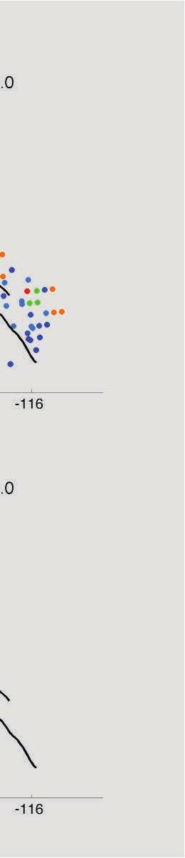
74

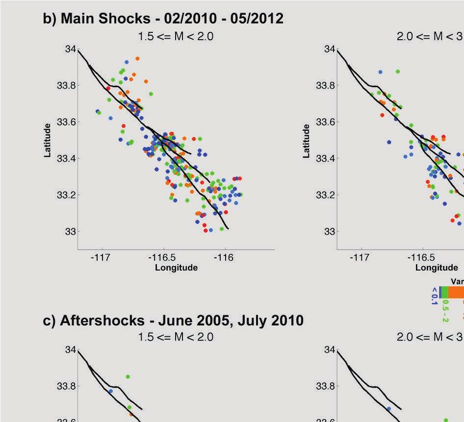
75

76 Figure 17: Phase 2 - Residual analysis for events. The residuals are analyzed for each event and color-coded according to res var, the variance of the residuals. Green dots show moderate variance and associate with events showing good fit to predictions, blue dots show small variance and associate with damped events (those events with overestimation of the predictions), and orange to red dots show large variance, associating with amplified events, in which the GMPE s underestimate the actual observations. a) All events, b e) M 1.5 3: b) main shocks, c) aftershocks June 2005 and July 2010, d) aftershocks March 2013 all stations, and e) aftershocks March 2013 old stations. The main feature of these figures is that the March 2013 shows very high variance in the source region for M 1.5 3, which seems to be a combination of source characteristics and fault zone new stations, and explains the high uncertainty seen in the March 2013 dataset.