ABSTRACT. Dissertation directed By: Professors William F. McDonough & Roberta L. Rudnick, Department of Geology

Transcription

1 ABSTRACT Title of Dissertation: GLOBAL AND REGIONAL REFERENCE MODELS FOR PREDICTING THE GEONEUTRINO FLUX AT SNO+, SUDBURY, CANADA Yu Huang, Doctor of Philosophy, 2013 Dissertation directed By: Professors William F. McDonough & Roberta L. Rudnick, Department of Geology Determining the radiogenic heat power that is driving plate tectonics and mantle convection is fundamentally important to understanding the Earth s heat budget and its thermal and chemical evolution. The radiogenic heat power is coupled to the chemical composition of the Bulk Silicate Earth (BSE), which has been debated for decades. Geoneutrinos produced by beta-minus decays in U, Th and K decay systems are correlated to the radiogenic heat power in the Earth. Measured geoneutrino signals at different locations can be used to investigate the distributions and abundances of U and Th, given appropriate reference Earth models. Here I construct both a global and regional scale reference model to predict the geoneutrino signal at the SNO+ detector in Sudbury, Canada. The primary objective of this dissertation is to predict the geoneutrino detection rate for this soon to be operational geoneutrino detector and evaluate its asymmetric uncertainty caused by the log-normal distributions of U and Th in the crust. The focus of both models are on the geoneutrino signal from the continental crust, which determines

2 SNO+ s sensitivity to the mantle geoneutrino signal, which is key to testing different BSE compositional models. The total geoneutrino signal at SNO+ is predicted to be TNU by combining the global and regional reference model predictions and assuming the contribution from continental lithospheric mantle and convecting mantle is 9 TNU. It is not feasible for SNO+, on its own, to provide experimental result that will determine the mantle geoneutrino signal and refine different BSE compositional models because of the large uncertainty associated with the crustal contribution. The regional crust study presented here lowers the uncertainty on the geoneutrino signal that originates from bulk crust when compared to the global reference model prediction ( TNU vs TNU). A future goal is to increase the resolution of the model in proximal area to the detector (e.g., 50 km by 50 km), which will further reduce the uncertainty. To obtain useful data on the mantle geoneutrino signal, detections of geoneutrinos carried out on the oceans, such as the proposed ocean-bottom Hanohano experiment, will be of significant scientific value.

3 GLOBAL AND REGIONAL REFERENCE MODELS FOR PREDICTING THE GEONEUTRINO FLUX AT SNO+, SUDBURY, CANADA By Yu Huang Dissertation submitted to the Faculty of the Graduate School of the University of Maryland, College Park, in partial fulfillment of the requirements for the degree of Doctor of Philosophy 2013 Advisory Committee: Professor William F. McDonough, Chair Professor Roberta L. Rudnick Professor Stephen T. Dye Professor Steven Shirey Professor Laurent G. J. Montesi Dean s Representative Professor Carter Hall

4 Copyright by Yu Huang 2013

5 Preface Some work reported in this dissertation was previously published, submitted, or is in preparation for peer-reviewed journals. The contributions of my collaborators, as well as reviewers and editors, are acknowledged in this thesis. ii

6 Dedication This dissertation is dedicated to my family, who has continuously provided courage to me from the beginning. In particular, to my wife, Tingting, and the greatest project of my life, my son Eric, today I dedicate them this dissertation, because without their support and love I would have not achieved my goal. I owe a great deal of debt and gratitude to my mom and dad. They were supportive of my decision to get a doctoral degree in geoscience overseas. Without their spiritual support, I would not be here today. I am very sorry for not being able to accompany them during their most difficult time, but just making this dedication of my dissertation. I also appreciate all the love and support from my sisters and parents-in-law. The important thing is not to stop questioning. -- Albert Einstein iii

7 Acknowledgements First and foremost, I must acknowledge all the effort that my advisors, Bill McDonough and Roberta Rudnick, have poured out to me during my Ph.D. study. They hold my hands and led me into this quite young neutrino geoscience field. I have enjoyed from the first touch of geoneutrinos until the completion of this dissertation. Beyond appreciating their effort to fly me up to a Star Alliance Gold member, I must thank them for teaching me how to be a good and successful scientist, from attitude and ethics of research. Their advice to think big and critically will benefit my entire life. I also owe a great deal of gratitude to Fabio Mantovani at University of Ferrara and INFN, who, with his students, Viacheslav Chubakov and Virginia Strati, served as my collaborators, co-authors, and friends. Without their work, I would not be able to achieve this stage today. I have enjoyed all the visits to Ferrara and the espresso coffee there. I thank Steve Shirey and Steve Dye for their collaboration to generate Chapter five and serving on my PhD examination committee. I appreciate the field trip to Sudbury led by Steve Shirey and John Ayer. I have enjoyed all scientific discussions with Steve Dye, which have encouraged me to understand geoneutrino physics deeper. I appreciate the willingness of Laurent Montesi to serve on my committee as well. I would also like to thanks Professor Carter Hall for taking interest in my research and joining my committee as the Dean s representative. I would like to acknowledge fruitful and insightful discussions with Vedran Lekic, Michael Evans, Eligio Lisi and Gerti Xhixha during my research. I am grateful to so many people for providing data for geoneutrino prediction: Mirko Reguzzoni and iv

8 Daniele Sampietro for sharing the GEMMA data, Andrew Kerr for providing a geochemical database for basaltic oceanic plateaus, John Ayer and Mike Easton for sharing their chemical composition data in the Canadian Shield, Richard Gaschnig for providing the tillite data, Trond Slagstad for sending the chemical data in Grenville Province, and Valentina Puchtel for her help during the dataset compilations. I am grateful for the help of Geology faculty and staff members, who made my life joyful at Maryland! Especially, thanks to Sandy Romeo, Michelle Montero and Todd Karwoski for their great support. I would like to thank various postdocs and graduate colleagues that overlapped with me at Maryland, who provided tremendous help academically and personally (in alphabetical order by last name): Rick Arevalo, Hailong Bai, Dana Borg, Huan Cui, Richard Gaschnig, Nick Gava, Jill Gribbin, Brain Harms, Su Li, Harry Lisabeth, Jingao Liu, Xiao-Ming Liu, Kristy Long, Yongbo Peng, Lin Qiu, N & M Sharps, Rose Smith, Lauren Stevens, Ming Tang, Lisa Walsh, Emily Worsham and the rest of the department. v

9 Table of Contents Preface... ii Dedication... iii Acknowledgements... iv Table of Contents... vi List of Tables... viii List of Figures... x Chapter 1: Introduction... 1 Chapter 2: Geoneutrino physics Introduction Geoneutrino production Geoneutrino oscillation Geoneutrino detection Detection Detectors and detection results Geoneutrino flux Chapter 3: A reference Earth model for the heat producing elements and associated geoneutrino flux Abstract Introduction Heat producing elements and Earth differentiation Geoneutrino Modeling the Earth's heat producing elements Methodology and reference states Selection of flux calculation sites Structure and mass of the crust The lithospheric mantle The sublithospheric mantle Compositions of Earth reservoirs The core BSE models and uncertainties Sublithospheric mantle (DM and EM) Continental lithospheric mantle (CLM) Crustal components, compositions and uncertainties Refined estimates for the composition of the deep continental crust and continental lithospheric mantle General considerations In situ velocity to rock type Rock type to chemistry Deep crust composition Average composition of peridotites and uncertainties vi

10 5. Methods of analysis and propagation of uncertainties Discussion Physical and chemical structure of the reference crustal model Geoneutrino flux and radiogenic heat power Conclusions Supplement material Chapter 4: Propagation of uncertainties by Monte Carlo simulation Abstract Introduction Derivative approximation method Monte Carlo simulation Examples Complicated non-linear combination function Non-Gaussian data distributions Conclusions Chapter 5: Regional study of the Archean to Proterozoic crust at the Sudbury Neutrino Observatory (SNO+), Ontario: Predicting the geoneutrino signal Introduction Motivation Building the model Geology framework of the regional crust Superior Province Grenville Province Southern Province and Sudbury Igneous Complex Paleozoic sedimentary units Simplified surface geology Geophysical 3-D model of the regional crust Geophysical model of boundary surfaces Geophysical model of regional upper crust Cross-checking the 3-D model Chemical composition of reservoirs Geoneutrino signal Discussion Heat production Mantle geoneutrino signal Conclusions Chapter 6: Summary and future work Bibliography vii

11 List of Tables Table 1.1: Different models of K, Th and U abundances and radiogenic power in the Bulk Silicate Earth (BSE)... 3 Table 2.1: Properties of 238 U, 235 U, 232 Th, and 40 K for atomic parameters, radiogenic heating and geoneutrino luminosity Table 3.1: Geoneutrino flux (no oscillation) at 16 geographic sites Table 3.2: Geoneutrino signal at four sites from each reservoir as in the global reference model Table 3.3: Global average physical and chemical properties of each reservoir as in the global reference model Table 3.4: Average seismic velocities and SiO 2 of amphibolite and granulite facies rocks Table 3.5: Average HPE abundances in amphibolite facies, granulite facies and peridotite rocks Table 3.6: Comparison of crustal thickness and mass between previous models and global reference model Table 3.7: Comparison of HPE abundances in continental crust between previous models and global reference model Table 3.8: Comparion of HPE abundances, K/U, Th/U and radiogenic heat power in bulk continental crust between previous models and global reference model Table 4.1: Sensitivity test for Monte Carlo simulation in Excel and MatLAB Table 5.1: Seismic lines used for modeling the regional crust viii

12 Table 5.2: Descriptive statistics of depth-controlling data points for boundary surfaces (TMC, TLC and MD) Table 5.3: Physical properties of three crustal reservoirs within the 3-D regional crustal model Table 5.4: Physical properties of seven sub-reservoirs in the upper crust within the 3-D regional crustal model Table 5.5: U and Th abundances in seven sub-reservoirs in the regional upper crust Table 5.6: Heat production and geoneutrino signal at SNO+ from each reservoir in the 3- D regional model ix

13 List of Figures Figure 2.1: 238 U decay chain Figure 2.2: 232 Th decay chain Figure 2.3: Geoneutrino intensity energy spectra Figure 3.1: Schematic structure of the global reference Earth model Figure 3.2: Distribution of continental crust thickness in three global crustal models and new reference model Figure 3.3: Seismic velocity vs. SiO 2 of amphobolite and granulite facies rocks Figure 3.4: Histogram of seismic velocity of amphibolite and granulite facies rocks Figure 3.5: Frequency distribution of U abundances of amphibolite facies rocks Figure 3.6: Box-and-Whisker diagram for HPE abundance of amphibolite and granulite facies rocks Figure 3.7: Thickness of crust and its uncertainty of global reference model Figure 3.8: Abundance of U and Th in middle and lower continental crust Figure 3.9: Geoneutrino signal at Earth's surface Figure 3.10: Predicted geoneutrino signals from the mantle and lithosphere Figure 4.1: Schematic illustration of Monte Carlo simulation Figure 4.2: Frequency distribution of output variable in example # Figure 4.3: Frequency distribution of output variable in example # Figure 5.1: Geophysical constraints on the 3-D regional model Figure 5.2: Simplified geological map of regional crust Figure 5.3: Maps of depth and associated uncertainty for inter-crustal boundaries: TMC, TLC and MD x

14 Figure 5.4: Six schematic crustal cross section in the regional crust Figure 6.1: Experimentally determined and theoritical predicted geoneutrino signals at KamLAND and Borexino xi

15 Chapter 1: Introduction Geoscientists aim to understand how the Earth operates, including the sources of its power for driving mantle convection, global plate tectonics, and the geodynamo. The prerequisite to understanding these fundamental questions associated with the Earth s heat engine is determining the Earth s energy budget, which is roughly a balance between secular cooling and radiogenic heat production. Determining the relative contribution of these two energy sources is fundamentally important for understanding Earth s dynamics and evolution history (e.g., Jaupart et al., 2007; Korenaga, 2008; Mareschal et al., 2012). The Earth s total surface heat flow is estimated to be between 42 and 47 TeraWatts (TW) (e.g., Sclater et al., 1980; Pollack et al., 1993; Jaupart et al., 2007; Davies and Davies, 2010). A significant fraction of the surface heat flow comes from radiogenic heat produced by the decay of radionuclides. Long-lived radionuclides, particularly 40 K, 232 Th and 235, 238 U, contribute more than 98% of the total radiogenic heat power within the planet and are therefore referred to as the heat producing elements (HPEs, namely U, Th and K) (e.g., Van Schmus, 1995; Fiorentini et al., 2007). While the surface heat flow is well characterized, estimates of how much radiogenic heat is generated in the Earth are associated with larger variations, reflecting the intensive debates regarding the chemical composition of bulk silicate Earth (BSE). The BSE is defined as the Earth s mantle immediately after segregation of the core, but before extraction of continental crust, which corresponds to the combined present-day crust and mantle. Methods used to estimate the chemical composition of the BSE are principally based on cosmochemical, geochemical, and/or geodynamical data or modeling (e.g., McDonough and Sun, 1995; Turcotte and Schubert, 2002; Javoy et al., 1

16 2010). However, radiogenic heat power generated in the Earth s interior based on different BSE compositional models varies by a factor of three (Table 1.1). Estimates of HPE abundances in the Earth are made via two approaches: 1) the geochemicalcosmochemical approach is based on a scenario for the origin of the Earth that entails the accretion of chondritic meteorites; and 2) a balance between the Earth s heat dissipation and production (geophysical model). Enrichment of U and Th in the BSE relative to that in chondritic meteorites is due to core formation and loss of volatile elements, assuming they do not significantly enter the core (e.g., Wheeler et al., 2006). The model of Javoy et al. (2010) envisages that the Earth accreted from enstatite chondrites, and suggests that the Earth s enrichment factor for the refractory lithophile elements (e.g., U and Th) is ~1.5. This enrichment factor reflects strictly the influence of core formation, as enstatite chondrites have low volatile element contents, like the Earth. The abundance of U in enstatite chondrite model is ~12 ng/g (or ppb) and the corresponding radiogenic heat power is ~11 TW, of which ~7 TW is coming from the continental crust (Huang et al., 2013, and references therein). For primordial Earth models built from carbonaceous chondrites (specifically CI chondrites, which has ~8 ppb of U), the enrichment factors range from ~2.2 (Lyubetskaya and Korenaga, 2007a) up to ~2.8 (Palme and O'Neill, 2003). These conventional geochemical estimates of the radiogenic heat power are ~20 TW (e.g., Hart and Zindler, 1986; McDonough and Sun, 1995; Palme and O'Neill, 2003). O'Neill and Palme (2008) proposed a depleted BSE compositional model, which has only 10 TW radiogenic heat power, based on a collisional erosion scenario, where an incompatible element enriched early crust was preferentially lost via early collisions. Parameterized mantle convection models (e.g., Turcotte and Schubert, 2002) relate 2

17 convection with heat loss by refining the mantle viscosity to describe the thermal evolution of the Earth. These models generally require higher abundances of HPEs in the Earth, which can release ~30 TW of radiogenic heat (Table 1.1). Table 1.1: Different models of K, Th and U abundances and radiogenic power in the bulk silicate Earth (BSE). Bulk Silicate Earth Models a O&P b J L&K AN M&S AL H&Z P&O T&S K c d Th U Th/U Enrichment e P (TW) a BSE mass is kg (Huang et al., 2013). b O&P (O'Neill and Palme, 2008); J (Javoy et al., 2010); L&K (Lyubetskaya and Korenaga, 2007a, b); AN (Anderson, 2007); M&S (McDonough and Sun, 1995); AL (Allègre et al., 1995); H&Z (Hart and Zindler, 1986); P&O (Palme and O'Neill, 2003); T&S (Turcotte and Schubert, 2002). c K is reported as µg/g; Th and U are reported as ng/g; Power is in TW (10 12 Watt). d Updated by Arevalo et al. (2009). e Enrichment refers to the enrichment factor of U and Th in the BSE relative to CI chondrites. Another parameter that describes the contribution of radiogenic heat to total heat flow is the Urey ratio (hereafter Ur), which is defined in two distinct ways. Geophysical models often refer to a convective Ur (or mantle Ur), defined as the ratio of radiogenic heat power in the modern mantle to the total mantle heat flow (i.e., total surface heat loss (47 TW) minus the radiogenic heat power in the crust (7 TW)). Geochemical studies focus on the bulk Earth Ur, or the ratio of Earth s radiogenic heat power over surface heat 3

18 loss. Current estimates of the convective Ur range from 0.2 to 0.7 (Korenaga, 2008). Determining the radiogenic heat power in the Earth or the convective Ur is needed in order to understand the dynamics and evolution of the convecting mantle. The abundances and distributions of HPEs in the crust, especially the continental crust, are not completely resolved. The continental crust, which constitutes only ~0.5 % (by mass) of the BSE, contains about one third of the Earth s total HPEs (e.g., Rudnick and Gao, 2003; Jaupart et al., 2007; Huang et al., 2013). The different models have roughly the same composition for the upper continental crust. However, for the deep crust, uncertainty about its composition (felsic or mafic) and radioactivity increases due to the limited amount of available samples and higher sampling bias. The abundances of HPEs in the deep crust correlate with its silicon content, which is a fundamental parameter to access the evolution of the continental crust (e.g., Rudnick and Gao, 2003; Hacker et al., 2011). If we can reduce the uncertainties on the abundances and distributions of the HPEs in the BSE, we will in turn be able to provide answers or new constraints on many long-lasting questions: 1) What is (or are) the right compositional model(s) for the BSE? 2) What type of chondrites is most likely to be the parent material of the Earth? 3) What are the chemical and thermodynamic processes that brought the Earth to its present state? 4) Is the mantle chemically or physically layered and is there a hidden reservoir of incompatible elements (including U and Th) in the deep mantle? 4

19 5) Given that primary melts of Earth s mantle must be basalt-like, how did the continental crust evolve to have an average andesite composition? Is the relamination model by Hacker et al. (2011) able to explain its chemical evolution? 6) Is there a significant amount of HPEs in the Earth s core? This list is only a few of the fundamental questions that can be asked about the Earth s interior. All involve the need to understand the concentration and distributions of HPE in the Earth. The new field of geoneutrino science (Dye, 2010, 2012; McDonough et al., 2012) holds the potential to address the above questions and to measure the Earth s radiogenic heat power. Geoneutrinos are electron antineutrinos naturally emitted in beta-minus decays ( n p + e + v e ) of terrestrial radionuclides and their daughter nuclides in the Earth. The main contributing nuclides to beta-minus decays include the HPEs, such as 238 U and 232 Th, and their decay products. Therefore, the geoneutrino signal is strictly dependent on the abundances and distributions of U and Th (as well as K), and consequently, on natural radioactivity. The possibility of remote sensing of HPEs in Earth s interior through geoneutrino at the Earth s surface was suggested nearly 50 years ago (e.g., Eder, 1966; Marx, 1969; Marx and Lux, 1970; Avilez et al., 1981; Krauss et al., 1984; Kobayashi and Fukao, 1991a; Raghavan et al., 1998; Rothschild et al., 1998). Particle physicists have recently demonstrated the detection of geoneutrinos at the Kamioka liquid scintillator antineutrino detector (KamLAND) (Araki et al., 2005; Abe et al., 2008; Gando et al., 2011; Gando et al., 2013) and the Boron Solar Neutrino Experiment (Borexino) detector (Bellini et al., 2010; Bellini et al., 2013a). SNO+, making use of the facility at the former Sudbury Neutrino Observatory (SNO) experiment at SNOLAB, is an antineutrino 5

20 detector that will become operational in 2014 and will have a significant signal-to-noise ratio for geoneutrino detection (Chen, 2006). As these three detectors are accumulating more and more geoneutrino event data, an updated reference model is highly desired that will assist in interpretation of the geoneutrino detection results (or counting rate), specifically, to place constraints on the abundances and distributions of HPEs in the Earth s interior. Previous reference models (e.g., Mantovani et al., 2004; Enomoto, 2005; Fogli et al., 2006; Dye, 2010) used the geophysical 2 2 crustal model (CRUST 2.0; Bassin et al., 2000; Laske et al., 2001), the preliminary reference earth model (PREM; Dziewonski and Anderson, 1981), and compositional models for the crust and mantle. The shared weakness of these earlier reference models is that no evaluation of uncertainties was carried out. This is particularly important for the crustal model, since the continental crust is estimated to contribute % of the total signals at the three detectors. Most compositional models for the crust and mantle lack uncertainties (e.g., lower crust composition estimated by Rudnick and Gao (2003); BSE compositional models). Therefore, the reference model used to interpret the future geoneutrino detection results should incorporate better evaluations of uncertainties associated with both the physical and chemical Earth models. Geoneutino measurements can be used to resolve different estimates of total radiogenic heat power (and in turn evaluating BSE compositional models), while the mantle s contribution to the total geoneutrino signal can be determined by subtracting the crustal contribution from the total signal (e.g, Dye, 2010). Whether the SNO+ detector has the sensitivity to determine the mantle geoneutrio signal depends on how accurate and precise the estimates of crustal contributions can be made. As highlighted by Araki et 6

21 al. (2005) and Chen (2006), geoneutrinos from sources within 500 km of a continental based detector contribute approximately 50% of the signal. Likewise, the local continental crust in the Canadian Shield is the dominant source for the geoneutrino signal at SNO+, and its geoneutrino contribution should be addressed carefully. Therefore, it is necessary to construct a detailed regional crustal model to characterize the abundances and distributions of U and Th around the SNO+ detector. The geoneutrino flux, and especially its uncertainty, can be predicted and then be used to extract the mantle signal. In this dissertation, I present new global and regional reference model for predicting the geoneutrino signal, and its uncertainty, at the SNO+ detector. The following four chapters address how the geoneutrino measurements are linked to the radiogenic heat power in the Earth, and how to construct both global and regional reference models for the coming SNO+ detector. Some chapters are papers that have either been published, have been submitted for publication, or are anticipated to be published. Chapter two reviews the properties and productions of geoneutrinos, their propagation through the Earth, the detection mechanism, recent experimental results, and approaches to predict the geoneutrino flux at Earth s surface based on geophysical and geochemical models. This chapter reviews how the geoneutrinos can serve as an independent probe into the deep Earth and provide an estimate of the Earth s radiogenic heat power. Chapter three presents an updated global reference Earth model for HPEs and the associated geoneutrino flux at various locations at the Earth s surface. The structure and composition of the outermost portion of the Earth, the crust and underlying lithospheric 7

22 mantle, is detailed in the reference model as this portion of the Earth has the greatest influence on the geoneutrino fluxes. Three existing geophysical models of the global crust are combined to reach an evaluation of the uncertainty of crustal thickness. In situ seismic velocities are used to estimate the composition of deep continental crust, employing new and updated compositional databases for amphibolite and granulite facies rocks in combination with laboratory ultrasonic velocities measurements. An updated xenolithic peridotite database is used to represent the average composition of continental lithospheric mantle. The asymmetrical uncertainties for radiogenic heat power and geoneutrino flux at the Earth s surfaces are calculated using by Monte Carlo simulations. This work has been published as an article entitled as A reference Earth model for the heat-producing elements and associated geoneutrino flux in Geochemistry, Geophysics and Geosystems by Huang, Chubakov, Mantovani, Rudnick and McDonough. Chapter four introduces a new method of using Monte Carlo simulation to determine the uncertainties of geochemical data populations with non-gaussian distributions. The commonly adopted approach to combine uncertainties is the derivative approximation, which is limited by its associated requirements that the linear approximation of the combination function is valid and the input variables have Gaussian distributions. In contrast to the traditional approach, the Monte Carlo simulation does not have such requirements, and provides a comprehensive and powerful method to propagate uncertainties with known distributions (not limited to Gaussian) and correlations. This chapter provides two simple cases (geochronology and ratio of incompatible elements) in which the Monte Carlo simulation demonstrates its advantage over the derivative approximation approach. 8

23 Chapter five describes a regional study of the Archean to Proterozoic crust around the SNO+ detector in order to predict the regional contribution to the geoneutrino signal. The most important goal of this study is to evaluate the possibility of extracting the mantle geoneutrino signal from the future experimental results in order to resolve different BSE compositional models. A 3-D regional crustal model for six 2 2 tiles centered at SNO+ is constructed. Available geological, geophysical, and geochemical information in this area is integrated into the model to describe the abundances and distributions of U and Th in the continental crust near SNO+. The geoneutrino flux from this regional crust is predicted by using the Monte Carlo simulation described in Chapter four to propagate asymmetrical uncertainties on U and Th abundances. Conclusions and future work directions are presented in Chapter six. 9

24 Chapter 2: Geoneutrino physics and radiogenic heat power 1 [1] Y. Huang created/wrote all the material in this chapter. 1. Introduction Geoneutrinos are electron antineutrinos emitted by beta-minus decays of naturally occurring radionuclides (e.g., U, Th, K and Rb). These long-lived radioactive elements also contribute a significant amount of radiogenic heat power to the Earth s energy budget. The inherent connection between geoneutrinos and radiogenic heat power in the Earth provides an independent approach to constrain the thermal and chemical evolution of this planet by counting geoneutrinos. Detection of geoneutrinos is now feasible due to two advances made by physicists in the last decade: 1) development of large (anti)neutrino detectors with low background and 2) understanding the oscillation phenomenon of these lightest of the known massive particles. To date, two different experiments at KamLAND and Borexino have provided constraints on the available radiogenic power to drive mantle convection and plate tectonics (Bellini et al., 2013a and references therein; Gando et al., 2013). A new detector, SNO+ at Sudbury, Canada, is scheduled to come online in late 2013 or early Some other experiments capable of detecting geoneutrinos have also been proposed. Compared to other emissions (e.g., noble gases, heat flow) from the Earth s interior, geoneutrinos provide information regarding global properties of the Earth instantaneously. This chapter reviews the properties of geoneutrino. It begins with a description of the production of these messengers from within the planet and the evaluation of radiogenic heat power and geoneutrino luminosity (section 2). Following 10

25 this are descriptions of geoneutrino oscillation (section 3) and current detection techniques (section 4). The final section describes how to predict geoneutrino flux arriving at the detectors. 2. Geoneutrino production Electron antineutrinos ( ν e ) are generated from the decay of neutron-rich nuclei, which are formed by nuclear fission processes and naturally synthesized in supernovae. Geoneutrinos are electron antineutrinos produced within the Earth by beta-minus decay when a neutron decays to a proton via the weak interaction, accompanied by emission of an electron ( e ) and release of decay energy ( Q β ), A A Z Z+ 1 ' ν e X X + e + + Q β (Eq. 2.1) where A is the mass number of nuclide X, and Z is the atomic number. Terrestrial isotopes of uranium (U), thorium (Th) and potassium (K) are the dominant sources of radiogenic power within the Earth, which drives mantle convection and plate tectonics. All three of these decay systems generate geoneutrinos (e.g., Van Schmus, 1995; Fiorentini et al., 2007; Dye, 2012; Šrámek et al., 2012): U Pb + 8α + 6e + 6ν MeV, U Pb + 7α + 4e + 4ν MeV, Th Pb + 6α + 4e + 4ν MeV, K Ca + e + ν MeV (89.3%), K + e Ar + ν MeV (10.7%) e e e e e (Eq. 2.2) The radiogenic heat generated per decay ( Q = Q Q ) is the energy difference between decay energy ( Q β ) and the energy that is carried away by antineutrinos ( Q ν ). h β ν 11

26 The production rate of radiogenic heat ( H ) and geoneutrino luminosity ( L ), per unit mass of each parent nuclide, can be calculated from (e.g., Dye, 2012) R where N A NAλQh H R =, µ (Eq. 2.3) NAλnν L =, µ (Eq. 2.4) is Avogadro s number, λ is decay constant, µ is molar mass, and n ν is number of geoneutrinos produced per decay chain. Table 2.1 presents the these quantities for 238 U, 235 U, 232 Th, and 40 K, as reported by Šrámek et al. (2012) and Dye (2012). Table 2.1: Properties of 238 U, 235 U, 232 Th, and 40 K for atomic parameters, radiogenic heating and geoneutrino luminosity. From Šrámek et al. (2012) and Dye (2012). 238 U 235 U 232 Th 40 K Natural isotopic fraction Molar mass µ (g mol -1 ) Decay constant λ (10-18 s -1 ) Decay energy Q β (10 12 J) Geonu energy Q ν (10 12 J) Radiogenic heating Q h (10 12 J) Radiogenic heat generation H R (µw kg -1 ) Geonu per chain n ν Geonu luminosity L (kg -1 µs -1 ) The total radiogenic heat production (µw) and geoneutrino luminosity (µs -1 ) of the Earth is directly tied to the mass of all these parent radionuclides: 12

27 H = m U + m U + m Th + m K (Eq. 2.5) R, ( ) ( ) ( ) ( ), L m U m U m Th m K = 74.6 ( ) ( ) ( ) ( ). (Eq. 2.6) By considering the natural isotopic fractions of the parent radionuclides, the above two equations can be rewritten in terms of the total masses of three elements (U, Th, and K, referred to as the heat producing elements): H R, = 98.5 m( U ) m( Th) m( K), (Eq. 2.7) L = 76.4 m( U ) m( Th) m( K). (Eq. 2.8) Considering the fact that, in the Earth, m(th)/m(u) 4, one expects approximately similar radiogenic heat power and geoneutrino luminosity (or flux) from U and Th. Current geoneutrino detection technology, which is based on the inverse beta reaction on a free proton (section 4), is only able to detect geoneutrinos emitted from the 238 U and 232 Th decay chains. Although 40 K is another plentiful geoneutrino source, the maximum energy of its geoneutrino is less than the energy threshold of the inverse beta reaction (1.806 MeV). The geoneutrinos from 235 U are only about 3% of those from 238 U (considering m( 238 U)/m( 235 U) = and plugging into Eq. 2.6), and they are normally ignored (the maximum energy is also below the detection threshold). The decay chain of 238 U to stable 206 Pb, which includes eight alpha decays and six beta decays, is shown in Fig Only three nuclides ( 234 Pa, 214 Bi and 206 Tl) in the chain yield geoneutrinos with energy larger than MeV and these three contribute to the detectable geoneutrino signal. However, the contribution of 206 Tl is negligible due to the very small occurrence probability. Th-232 decays to 208 Pb through six alpha decays and 13

28 four beta decays (Fig. 2.2). The only two parent nuclides with detectable geoneutrinos are 228 Ac and 212 Bi. The energy spectra of geoneutrinos from different decays or decay chains are determined by integrating energy spectra of all beta decays with information on branching ratios, decay constants and fractional intensities (Enomoto, 2005; Fiorentini et al., 2007). Dye (2012) recalculated geoneutrino intensity energy spectra per decay for 238 U, 235 U, 232 Th, and 40 K (Fig. 2.3). On average, approximately 2/3 of the decay energy of the corresponding beta decay is carried away by the geoneutrino (Van Schmus, 1995). 3. Geoneutrino oscillation Neutrinos and geoneutrinos are associated with three different lepton flavors (eigen-state of weak interaction), namely, electron, mu, and tau (e, µ, τ). Neutrino oscillation is a quantum mechanical phenomenon first hypothesized by Bruno Pontecorvo (Pontecorvo, 1957), which describes the possibility that a neutrino created with a specific lepton flavor will later be observed to have a different flavor. This oscillation phenomenon arises from the mixture between the three flavors and mass eigenstates, and has now been observed for solar, atmospheric, reactor, and accelerator-produced neutrinos. The formalism for neutrino oscillation is beyond the scope of this chapter, and for a review see Kuo and Pantaleone (1989). Geoneutrinos are generated in the Earth as electron antineutrinos, but the detector receives a flux of mixed electron, mu, and tau antineutrinos after their propagation in the Earth. As only electron antineutrinos are detectable by inverse beta reaction, neutrino oscillation diminishes the observable geoneutrino signal, depending on the geoneutrino energy and distance travelled (Araki et al., 2005). The three-flavor survival probability of 14

29 an electron antineutrino of energy E ν after a traveling distance L is (Dye, 2012; Šrámek et al., 2012): 3ν Pee ( Eν, L) = 1 {cos θ13 sin (2 θ12)sin 21 + sin (2 θ13)[cos (2 θ12)sin 31 + sin (2 θ12)sin 32]} (Eq. 2.9) where θ 12 and θ 13 are mixing angles, δ mij [ev ] L[m] ij ( Eν, L) =, (Eq. 2.10) E [MeV] ν and δ m = m m is the mass-squared difference between two mass eigenstates. Given ij i j the determined δm δm δm (Nakamura, 2010; Dye, 2012), the three-flavor survival probability for electron antineutrinos (Eq. 2.9) can be simplified to 3ν Pee ( Eν, L) = 1 [cos θ13 sin (2 θ12)sin 21 + sin (2 θ13)], (Eq. 2.11) 2 and reorganized to (Gando et al., 2013) P ( E, L) = cos θ P ( E, L) + sin θ, (Eq. 2.12) 3ν 4 2ν 4 ee ν 13 ee ν 13 where P ( E, L) = 1 sin (2 θ )sin, (Eq. 2.13) 2ν 2 2 ee ν which is the two neutrino survival probability. The oscillation length for geoneutrinos with energies between 1.8 MeV to 3.3 MeV is only about 60 to 110 km (Šrámek et al., 2012), which is only about 1-2% of the Earth s radius. For this reason, the average two-flavor survival probability for geoneutrinos is usually simplified, introducing only minimal error, to 15

30 2ν 1 2 Pee ( Eν, L) = 1 sin (2 θ12), (Eq. 2.14) 2 and the corresponding simplification to three-flavor survival probability to 3ν Pee ( Eν, L) = cos θ13(1 sin (2 θ12)) + sin θ13. (Eq. 2.15) 2 The most recent experimental determination for the θ 12 and θ13 mixing angles is by Gando et al. (2013). They reported tan θ = and sin θ = 0.023, the latter of which is in agreement with Daya Bay (An et al., 2012) and RENO (Ahn et al., 2012) experiments. Plugging these mixing angles into Eq. 2.15, the average three-flavor survival probability of geoneutrinos is 0.551± (Gando et al., 2013). The less than 3% uncertainty on the average survival probability is completely negligible comparing to the uncertainty associated with global reference modeling of geoneutrino flux or geoneutrino signal measurements. However, when determining the contribution to total geoneutrino flux at detectors from surrounding local crust within oscillation length, the error introduced by taking the average survival probability could be significant. For locally-derived geoneutrinos, Eq or 2.12 should be used in combination of an estimate of the energy and flight distance of geoneutrinos. The above discussions regarding neutrino oscillation or survival probability of geoneutrinos are based on the assumption that they are propagating through a uniform medium, which is not exactly true for the Earth, as the density is not constant. The MSW (Mikheyev Smirnov Wolfenstein) effect (Wolfenstein, 1978; Kuo and Pantaleone, 1989) describes the effect of non-uniform matter on the behavior of neutrinos. Enomoto (2005) numerically tracked such an effect, and discovered that the influence on the average 16

31 survival probability is about 2%. Thus, in geoneutrino flux predictions presented here (Chapter 3 and 5), I do not take this negligible matter effect into account. 4. Geoneutrino detection 4.1. Detection Although the geoneutrino flux at the Earth surface is at the level of 10 6 cm -2 s -1, the first experimental observation of geoneutrinos was not made until 2005 (Araki et al., 2005). The challenge is due to the fact that antineutrinos only interact with matter through the weak interaction, which has a very small probability. Currently, only two operating (anti)neutrino detectors, KamLAND and Borexino, are capable of counting geoneutrinos and have successfully measured the geoneutrino flux at Earth surface (Araki et al., 2005; Bellini et al., 2010; Gando et al., 2011; Bellini et al., 2013a; Gando et al., 2013). Both experiments employ the same detection mechanism as that employed by Reines and Cowan (1953) in their pioneering experiment, referred to as the inverse beta decay reaction. During this process, an electron antineutrino scatters on a free proton in organic scintillating liquid, and produces a positron and a neutron, + ν e + p e + n. (Eq. 2.16) The kinematic threshold of this interaction is MeV, which is determined by the mass difference between neutron plus electron and proton. Thus, only a small fraction of geoneutrinos produced within 238 U and 232 Th decay chains, and none from 235 U or 40 K decay, can be detected via this reaction. The positron then annihilates with an electron within few nanoseconds, and emits two MeV gamma-rays. The kinetic energy of the positron and the energy of the two gamma rays are detected by the surrounding PMTs (photomultiplier tubes) as a 17

32 prompt signal. The visible energy of the prompt signal E prompt scales with the energy of incident antineutrino, Eprompt = 0.784MeV. The momentum of the incident E ν antineutrino transfers primarily to the neutron, which is thermalized and captured by another proton to form deuterium within scintillating liquid, within a mean lifetime of µs. The neutron capture is characterized by the emission of a 2.2 MeV deexcitation gamma ray, which is the delayed signal. The spatial and temporal coincidence of the prompt and delay signal provides a strong selection criterion for electron antineutrino candidates and allows them to be distinguished from most background sources. The background signal for geoneutrino observations includes nuclear reactor antineutrinos, fast neutrons produced by cosmic muons, interactions from neutron-rich nuclides ( 9 Li and 8 He, 13 C(α, n) 16 O), and other accidental coincidences. Among these background sources, the nuclear reactor antineutrino signal can be predicted and subtracted from total electron antineutrino events. This is achieved by calculating the expected number of events and corresponding energy spectra of electron antineutrinos from all running nuclear reactors. The energy spectrum of reactor antineutrinos overlaps that of geoneutrinos and extends up to about 8 MeV. Therefore, any antineutrino candidates with energy above the geoneutrino end point provide more constraints on the nuclear reactor antineutrino background. Cosmogenic background sources, such as fast neutrons or 9 Li and 8 He, are largely eliminated by the overburden of rocks above the detectors, which serve as an attenuation to reduce the muon flux. Careful calibration of the contribution from cosmogenic background must be modeled by Monte Carlo simulations. 18

33 Other background sources associated with the radioactive contaminants in the detector system (including scintillator, construction materials, PMTs, etc.) can be determined by measurement of the radioactivity in the system, and further reduced by purification of detector components. A more complete discussion of background sources is presented in Dye (2012) and in a new review by Bellini et al. (2013b). During the neutron thermalization process, the emitted neutron, which has received a low energy nudge from the geoneutrino, loses its directional information, and consequently carries next to no directionality data. The cross section of the inverse beta decay reaction is estimated to be ~10-43 cm 2, corresponding to the energy range of geoneutrinos (Dye, 2012). Given that the surface geoneutrino flux above the threshold energy is ~10 4 cm -2 s -1, a large detector is required to provide free protons (~10 32 ; 1 kiloton size of liquid scintillator) to realize a modest counting rate (~10 y -1 ). Future efforts on geoneutrino detection include, but are not limited to, accumulation of more geoneutrino counts to increase the statistics, creation of a network of geoneutrino observatories, development of new detection mechanisms to retrieve directionality of incident geoneutrinos, and detection of geoneutrinos from 40 K and 235 U. It will be of great value to have SNO+, the third scintillator detector capable of geoneutrino measurement in Canada, on line. This detector will have a higher geoneutrino counting rate due to its size and surrounding thick continental crust, and will provide information regarding the radioactivity of the Canadian Shield Detectors and detection results KamLAND (Kamioka Liquid-scintillator ANtineutrino Detector) in Japan and Borexino in Italy are the only two operating detectors making geoneutrino measurements 19

34 right now. Both contain large volumes of liquid scintillator, are monitored by surrounding inward facing PMTs, and are operated underground to reduce the incoming cosmogenic muon flux. Other scientific objectives are carried out at these two detectors while counting geoneutrinos, such as investigation of neutrino oscillation, nucleon decay, astrophysics, etc. In this section, the very basic geometrical structures of the two detectors and the coming SNO+ detector will be reviewed first, and the most recent geoneutrino detection results will be summarized. KamLAND, located in the Kamiokande-Mozumi mine in central west Japan, was designed to study reactor antineutrinos. It contains 1 kiloton liquid scintillator composed of 80% of dodecane (diluent), 20% of pseudocumene and 1.36 g liter -1 of diphenyloxazole (PPO, scintillating fluorophore molecule). All the liquid scintillator is contained in a 6.5 m radius spherical balloon monitored by ~1900 PMTs installed on the wall of a 9 m radius spherical stainless-steel tank. Between the inner balloon and the spherical tank, a fluid composed of 57% isoparaffin and 43% dodecane oils acts as a buffer. Coverage area of PMTs is ~34% of the total surface area of the tank. Further description of KamLAND experiment can be found in Enomoto (2005). Borexino is a 278-ton liquid scintillator detector located in the underground laboratory of Gran Sasso, central Italy. The scintillator is made of pseudocumene and PPO at a concentration of 1.5 g liter -1. A 6.85 m radius stainless steel sphere supports ~2200 PMTs to monitor the 4.2 m radius inner vessel, which is surrounded by 1050 m 3 pseudocumene. The optical coverage at Borexino is ~30% (Alimonti et al., 2009). Due to its smaller volume of liquid scintillator compared to KamLAND, the Borexino detector 20

35 has a lower geoneutrino counting rate, as the surface geoneutrino flux is similar at the two sites. SNO+ (Sudbury Neutrino Observatory+) is a follow-up experiment to SNO (Sudbury Neutrino Observatory) at SNOLAB near Sudbury, Ontario, Canada. Replacing the ~1 kiloton heavy water in SNO, SNO+ is filled with ~780 tons of liquid scintillator, which consists of CH 2 -based linear alkylbenzene doped with PPO, in a 6 m radius acrylic sphere. The inner active volume is shielded by ultra-pure water and monitored by ~9000 PMTs. Because SNO+ is located in thick continental crust, the expected geoneutrino counting rate is high, in principle 20 counts per year. The first geoneutrino experimental measurement was provided by KamLAND in 2005 (Araki et al., 2005). Later, Abe et al. (2008) and Gando et al. (2011) reported more geoneutrino observations at KamLAND. One of the most important discoveries is that the null hypothesis for geoneutrino is disfavored at the % confidence level. Further summary of the previous datasets is presented by Šrámek et al. (2012). In 2013, new data from KamLAND (Gando et al., 2013) encompassed a period (351 days) with reactor-off activity following the Fukushima nuclear accident in March The data are based on a total live-time of 2991 days from March 9, 2002 to November 20, Using a fiducial scintillator volume with 6.0 m radius, the total exposure is (4.90±0.10) target-proton-year. The total number of antineutrino candidates, after passing all selection criteria, is The overall background for electron antineutrinos in the energy range between 0.9 MeV and 8.5 MeV is determined to be 364.1±30.5. The 13 C(α,n) 16 O background was reduced by a factor of 10 after the purification of the liquid scintillator. The reactor antineutrino background is expected to 21

36 be 3564±145 (without oscillation). By assuming a Th/U mass ratio of 3.9, the total number of geoneutrino events from U and Th is , which corresponds to a flux of (3.4±0.8) 10 6 cm -2 s -1. The null hypothesis for geoneutrino has a probability of With the Earth model proposed by Gando et al. (2013), the new KamLAND geoneutrino flux translates into a radiogenic power of TW from U and Th. Examining all four data releases of geoneutrino measurement, there is a decreasing trend for the central value of the determined geoneutrino flux or radiogenic heat power in the Earth. However, considering uncertainty, the results all overlap. The Borexino collaboration provided their first geoneutrino observation at 4σ in 2010 (Bellini et al., 2010). Compared to KamLAND, Borexino benefits from cleaner detector components and greater distance to nuclear reactors, while its smaller size is the primary factor that limits accumulation of geoneutrino events. An update from 2013 (Bellini et al., 2013a) is based on data from December 2007 to August 2012, increasing the exposure from ton-year (or proton-year) to (613±26) ton-year (or (3.69±0.16) proton-year) after the selection cuts. After passing all selection criteria for electron antineutrinos, they identified 46 electron antineutrino candidates (25 in the geoneutrino energy window). Antineutrinos from nuclear reactors are the main background to geoneutrinos. The number of expected reactor antineutrinos is 33.3 ±2.4 events for the determined total exposure. Other background sources are reduced to almost negligible levels, and, in total, are 0.70±0.18 events for the whole period (for details, see Bellini et al., 2013a). By fixing Th/U mass ratio at 3.9, and applying unbinned maximal likelihood fit for the geoneutrino events and reactor antineutrino events, the best fit value 22

37 is 14.3±4.4 events for geoneutrinos. The null hypothesis for geoneutrino has a probability of Geoneutrino flux The fully oscillated differential geoneutrino flux dφi de ν from source radionuclide I at the detector is given by the following integration (Enomoto, 2005) dφi dn( Eν ) ai( L) ρ( L) = Ai P ( E, L ) dv deν de ν 4π L 3ν 2 ee ν, (Eq. 2.17) where Ai is the activity of the source I per unit mass, dn( Eν ) de ν is the intensity energy spectrum of source I, ai ( L) is the concentration of source I at position L from the detector, ρ( L) is the density at position L from the detector, and 3 ν P ( E, L) is the threeflavor electron (anti)neutrino survival probability as described in section 3, with energy E ν and distance between source and detector L. The integration is made over all entire ee ν volume of Earth. The total flux is an integration of the differential flux over the full energy spectrum, dφ max i φ i = de 0 ν. (Eq. 2.18) deν When dealing with a spatial integration that has a much larger scale than geoneutrino oscillation length (~100 km), the survival probability can be well averaged without introducing significant error. Under this assumption, Eq could be simplified to 23

38 3ν ai ( L) ρ( L) φi = Ai ni Pee dv, (Eq. 2.19) 2 4π L where n i is the total number of geoneutrinos per day of source I and three-flavor survival probability for geoneutrinos. 3 P ν ee is the average To predict the geoneutrino flux from a domain with uniform composition, Eq is further simplified to 3ν ρ( L) φi = Ai ni Pee a dv. (Eq. 2.20) 2 4π L For a uniform density spherical shell bounded by radii r 1 and r 2, which are both smaller than the detector s point radius R (Earth s radius), the integral in Eq can be calculated exactly in this simplified scenario 2 ρ( L) dv ρ r2 2 sin dr π d π d r ϑ = ϑ ϕ r π L π R + r 2 Rr cosϑ ρr r r r R+ r r R+ r = [2 (1 ) ln( ) + (1 ) ln( )]. 4π R 2 2 R R r2 R R r1 (Eq. 2.21) When trying to estimate the geoneutrino flux from non-uniform domains with scales larger than oscillation length, it is desirable that the domain is divided into a set of spatially defined small voxels, and assigned information, such as abundance for source radionuclide, density, distance to detector and volume of each voxel. Chapter 3 describes a global reference model for geoneutrino flux at Earth s surface with a focus on the contribution from bulk continental crust. The contribution to the geoneutrino flux at SNO+ from local continental crust is estimated in chapter 5. Due to the heterogeneous 24

39 structure of continental crust, Eq is utilized to perform the prediction of geoneutrino flux by integrating the contribution from each small voxel. 25

40 Fig. 2.1: The 238 U decay chain. Decay energy is listed in kev. The two gray boxes highlight the two parent nuclides ( 234 Pa and 214 Bi) that generate currently detectable geoneutrinos from this decay chain. Adopted from Fiorentini et al. (2007), with updates based on the Chart of the provided by the National Nuclear Data Center. 26

41 Fig. 2.2: The 232 Th decay chain. Decay energy is listed in kev. The two gray boxes highlight the two parent nuclides ( 228 Ac and 212 Bi) that generate currently detectable geoneutrinos from this decay chain. Adopted from Fiorentini et al. (2007), with updates based on the Chart of the provided by the National Nuclear Data Center. 27

42 Fig. 2.3: Geoneutrino intensity energy spectra per decay for 238 U, 235 U, 232 Th, and 40 K. The area below each curve integrates to the number of geoneutrinos emitted per decay. The dashed line is the 1.8 MeV energy threshold of the inverse beta decay reaction used in current detectors. Figure from Dye (2012). 28

43 Chapter 3: A reference Earth model for the heat producing elements and associated geoneutrino flux 1,2 [1] This chapter has been published as: Huang, Y., Chubakov, V., Mantovani, F., Rudnick, R.L., McDonough, W.F., A reference Earth model for the heat-producing elements and associated geoneutrino flux. Geochemistry, Geophysics, Geosystems 14, , doi: /ggge [2] R.L. Rudnick, W.F.McDonough, F. Mantovani developed the motivation and fundamental idea; Y. Huang compiled all the databases used in the study with the help of V. Puchtel; Y. Huang, V. Chubakov, and F. Mantovani constructed the physical model and performed all calculations; all coauthors contributed to the text, tables and figures; Y. Huang managed the editing and submission. Abstract The recent geoneutrino experimental results from KamLAND and Borexino detectors reveal the usefulness of analyzing the Earth s geoneutrino flux, as it provides a constraint on the strength of the radiogenic heat power and this, in turn, provides a test of compositional models of the bulk silicate Earth (BSE). This flux is dependent on the amount and distribution of heat producing elements (HPEs: U, Th and K) in the Earth s interior. We have developed a geophysically-based, three-dimensional global reference model for the abundances and distributions of HPEs in the BSE. The structure and composition of the outermost portion of the Earth, the crust and underlying lithospheric mantle, is detailed in the reference model, this portion of the Earth has the greatest 29

44 influence on the geoneutrino fluxes. The reference model combines three existing geophysical models of the global crust and yields an average crustal thickness of 34.4±4.1 km in the continents and 8.0±2.7 km in the oceans, and a total mass (in kg) of oceanic, continental and bulk crust is 0.67±0.23, 2.06±0.25 and 2.73±0.48, respectively. In situ seismic velocity provided by CRUST 2.0 allows us to estimate the average composition of the deep continental crust by using new and updated compositional databases for amphibolite and granulite facies rocks in combination with laboratory ultrasonic velocities measurements. An updated xenolithic peridotite database is used to represent the average composition of continental lithospheric mantle. Monte Carlo simulation is used to predict the geoneutrino flux at 16 selected locations and to track the asymmetrical uncertainties of radiogenic heat power due to the log-normal distributions of HPE concentrations in crustal rocks. 1. Introduction Determining the Earth s heat budget and heat production is critical for understanding plate tectonics and the thermal evolution of the Earth. Recent detection of geoneutrinos (electron anti-neutrinos generated during beta decay) offers a means to determine the U and Th concentrations in the Earth that is complementary to traditional cosmochemical or geochemical arguments (Dye, 2010). However, since all three existing geoneutrino detectors are currently located within the continental crust (two in operation, another coming on line in 2014), the crustal contribution, which dominates the geoneutrino signal, must be subtracted in order to determine the signal from the mantle and core (Dye, 2012; Fiorentini et al., 2012; Šrámek et al., 2013). 30

45 Here we develop a three-dimensional global reference model that describes the inventory and distribution of the heat producing elements (HPEs: U, Th and K) in the bulk silicate Earth (BSE), along with uncertainties. The greatest resolution of the model resides in the outermost portions of the Earth the crust and underlying lithospheric mantle, from whence the largest portion of the surface flux originates Heat producing elements and Earth differentiation Radioactivities of U, Th and K contribute about 99%, with a relative contribution of approximately 2:2:1, of the total radiogenic heat power of the Earth. Although the heat production rate for unit mass of Rb at natural isotopic abundance is higher than K, the contribution of Rb to the total radiogenic heat power is expected to be less than 1% (Fiorentini et al., 2007), given the relative decay rates, and a K/Rb ratio of ~400 in the BSE (McDonough and Sun, 1995). The other elements, such as La, Sm, etc., make negligible contributions to the total radiogenic power. Uranium and Th are refractory lithophile elements, while K is a volatile lithophile element. The lithophile classification means that HPEs are expected to reside in the rocky portion of the Earth (Goldschmidt, 1933), though some have speculated that U and K may become slightly siderophile or chalcophile at high temperatures and pressures, and thus, may enter the Earth s core (e.g., Lewis, 1971; Murrell and Burnett, 1986; Murthy et al., 2003). The refractory nature of U and Th means that the Earth should have accreted with the full solar complement of these elements, whereas the volatility of K has led to its depletion in the Earth relative to the Sun and primitive chondritic meteorites (e.g., McDonough, 2003). Thus, the concentration of K in the Earth is inferred from analyses of geological samples and its behavior relative to refractory elements. 31

46 Uranium, Th and K are all highly incompatible elements (defined as having crystal/melt partition coefficients much less than one), and, thus, are concentrated in melts relative to residues during partial melting. The Earth has experienced irreversible differentiation via melting and the ascent of these melts towards the surface, leading to the concentration of these elements in the outermost-layers of the planet. Thus, although the continental crust comprises only ~0.5% of the mass of the BSE, it contributes almost one third of the total radiogenic heat power, and refining the composition of the continental crust is an essential prerequisite to using geoneutrinos to see into the deeper levels of the Earth. Compositional models for the BSE vary by nearly a factor of three in their U content (i.e., ~10 ng/g (O'Neill and Palme, 2008; Javoy et al., 2010), ~20 ng/g (Hart and Zindler, 1986; Allègre et al., 1995; McDonough and Sun, 1995; Palme and O'Neill, 2003; Lyubetskaya and Korenaga, 2007a, b), and ~30 ng/g (Turcotte et al., 2001; Turcotte and Schubert, 2002; Anderson, 2007)). These models generally agree on a Th/U of 3.9 and a K/U of 14,000 (Arevalo et al., 2009). Compositional models for the continental crust (see summary in Rudnick and Gao (2003)) predict a U content of 1100 to 2700 ng/g, implying that anywhere between 30 and 45% of the budget of HPEs is stored in this thin skin of crust and that it is more than ~100-fold enriched over the modern mantle (i.e., ~13 ng/g of U), assuming a geochemical model for the BSE of McDonough and Sun (1995). Geoneutrino data, when available for several sites on the Earth, should be able to define permissible models for the BSE and the continental crust Geoneutrinos 32

47 The Earth is an electron antineutrino star that emits these nearly massless particles at a rate of ~10 6 cm -2 s -1 (e.g., Kobayashi and Fukao, 1991b; Mantovani et al., 2004; Enomoto et al., 2007; Fiorentini et al., 2007). Geoneutrinos are electron antineutrinos produced within the Earth by beta-minus decay when a neutron decays to a proton via the weak interaction. This decay process, in which a down quark transforms to an up quark, is mediated by the emission of a W - boson along with an electron, and a charge neutral electron anti-neutrino. Because of their vanishingly small cross-section for interaction, ~10-44 cm 2, matter is virtually transparent to these particles and they have about a 50% chance of passing through a light-year of lead without interaction. By comparison, the fusion processes inside the core of the Sun produce neutrinos, the anti-matter lepton counterpart of antineutrinos, which bathe the Earth s surface with a flux that is ~10 4 greater than the geoneutrino flux (Bahcall et al., 2005). The term geoneutrino distinguishes natural emissions of electron antineutrinos from those radiated from nuclear reactors. To date, geoneutrino flux measurements have been made at two detectors, KamLAND, at the Kamioka mine in Japan (Araki et al., 2005; Gando et al., 2011; Gando et al., 2013), and Borexino, at the Gran Sasso underground laboratories in Italy (Bellini et al., 2010; Bellini et al., 2013a), and provide constraints on the quantities of U and Th inside the Earth. The SNO+ detector at the Sudbury Neutrino Observatory, Canada (Chen, 2006), will come on-line in 2014 and will deliver significant new data on the geoneutrino flux from the Archean Superior Craton and surrounding North American plate. 33

48 Geoneutrinos originating from U and Th can be distinguished based on their energy spectra, e.g., geoneutrinos with E > 2.25 MeV are produced only in the 238 U chain (e.g., Araki et al., 2005). Liquid scintillator detectors work by sensing light generated during antineutrino-proton interactions: v e + p e + + n, when the v e has MeV energy, which is the energy needed to transform the proton, p, to a positron e + and a neutron, n. Of the total geoneutrino flux, only small portions of antineutrinos generated in the 238 U and 232 Th decay chains can be detected by this mechanism. The hydrogen nuclei, which are in abundant supply in hydrocarbon (C n H 2n ) based liquid scintillator detectors, act as the target for transiting antineutrinos. The directionality of antineutrinos is presently undetectable and, thus, the detectors are sensitive only to the integrated flux. Fortunately, because the geoneutrino flux at a detector decreases with distance from the source via the inverse square law, geoneutrinos can be used to detect regional differences in the distribution of U and Th in the continents, and, in principle, large-scale features in the mantle (Dye, 2010; Šrámek et al., 2013). Thus, accurate and precise detection of the surface flux of geoneutrinos, coupled with geochemical and geophysical models of local and global crust, will enable quantitative tests of compositional models of the planet Modeling the Earth s heat producing elements We can model the Earth s geoneutrino flux by assigning physical and chemical data to a set of spatially defined voxels (a volume element, comparable to a threedimensional pixel). Such a model can be compared to surface heat flow measurements and various mass balance models for the composition of the Earth and its internal reservoirs (i.e., crust, mantle, and core). Towards this goal, an enormous amount of geophysical and geochemical data have been collected and shared on line in the past few 34

49 decades. This information can be integrated into a broader framework in order to evaluate the nature and or existence of planetary features, such as chemical compositions of thermochemical piles in the mantle (Šrámek et al., 2013), the characteristics of a residual layer from a basal magma ocean (Labrosse et al., 2007; Lee et al., 2010), and/or the presence of an early Earth enriched reservoir that was sequestered at the core-mantle boundary (Boyet and Carlson, 2005). Future geoneutrino observations will bring clarity to the debates regarding the mantle Urey ratio (the ratio of radiogenic heat in the mantle to total mantle heat flux) and the forces driving plate tectonics and mantle convection (e.g., Labrosse and Jaupart, 2007; Korenaga, 2008). These data will also define aspects of the Earth s thermal evolution. To build the reference crustal model, we combine (1) geophysical information from seismic refraction measurements (Laske and Masters, 1997; Bassin et al., 2000), surface wave dispersion data (Shapiro and Ritzwoller, 2002) and gravity anomalies observations (Reguzzoni and Tselfes, 2009; Negretti et al., 2012), (2) estimates of the average compositions of the upper continental crust(rudnick and Gao, 2003), global sediments (Plank, 2013) and oceanic crust (White and Klein, 2013), (3) laboratory ultrasonic measurements of deep-crustal rock types, and (4) new and updated geochemical compilations for deep crustal rocks and lithospheric peridotites to provide new insights on the composition of the deep crust and continental lithospheric mantle (CLM). In order to make more accurate predictions of the geoneutrino flux at current detectors and possible future detector sites, we define the mass and geometry of continental crust, quantify the amount and distribution of the HPEs and characterize their lateral and vertical variations in the crust. We also provide uncertainties for all estimates. 35

50 For the first time, the geoneutrino flux originating from the CLM is estimated. Collectively, this model allows the geoneutrino flux from the deep Earth to be defined more accurately, given that a large proportion of total signal at any given detector located in the continental crust is derived from this thin outer crustal layer. 2. Methodology and reference states Here we describe the Earth as the sum of its metallic, silicate, and hydrospheric shells. The silicate shell of the Earth (equivalent to the BSE) is considered to be the main repository of HPEs, and we focus on understanding internal differentiation of this region (Fig. 3.1). The BSE is composed of five dominant domains, or reservoirs: the DM (Depleted Mantle, which is the source of mid-ocean-ridge-basalts -- MORB), the EM (Enriched Mantle, which is the source of Ocean Island Basalts -- OIB), the CC (continental crust), the OC (oceanic crust), and the lithospheric mantle (LM). It follows that BSE = DM + EM + CC + OC + LM. The modern convecting mantle is composed of the DM and the EM. We do not include a term for a hidden reservoir, which may or may not exist in the BSE; its potential existence is not a consideration of this paper Selection of flux calculation sites Although geoneutrinos can be measured, in principle, anywhere on the Earth, the experiments need to be carried out in underground (or underwater) laboratories in order to shield detectors from cosmic radiation; only a few locations therefore have particular experimental interest. We have calculated the fluxes at 16 sites where the exploration of the Earth through geoneutrinos is either currently underway (Kamioka, Japan, with the KamLAND experiment (Araki et al., 2005; Gando et al., 2011); Gran Sasso, Italy, with 36

51 the Borexino experiment (Alvarez Sanchez et al., 2012); Sudbury, Ontario, Canada, with the SNO+ experiment (Chen, 2006)), or where such experiments have been proposed or could be planned (Table 3.1). Hawaii (Hanohano (Dye, 2010)), Baksan (Baksan Neutrino Observatory (Buklerskii et al., 1995)), Homestake (Deep Underground Science and Engineering Laboratory (Tolich et al., 2006)), Curacao (Earth AntineutRino TomograpHy (De Meijer et al., 2006)) and Daya Bay (Daya Bay II (Wang, 2011)) are all sites that have been proposed for constructing liquid scintillator detectors capable of detecting geoneutrinos. LAGUNA (Large Apparatus studying Grand Unification and Neutrino Astrophysics) is looking for the best site in Europe where the LENA (Low Energy Neutrino Astronomy) experiment (Wurm et al., 2012) could be built: seven prospective underground sites in Europe (Pyhasalmi, Boulby, Canfranc, Fréjus, Slanic and SUNLAB (see LAGUNA website)) are being investigated. Finally, we also include the sites where the maximum and minimum geoneutrinos signal on the Earth s surface is expected: the Himalaya and Rurutu Island (Pacific Ocean), respectively Structure and mass of the crust In 1998, the CRUST 5.1 model (Mooney et al., 1998) was published as a refinement of the previous 3SMAC model (Nataf and Richard, 1996). The model included 2592 voxels on a 5 5 grid, and reported the thickness and physical properties of all ice and sediment accumulations and of normal and anomalous oceanic crust. Vast continental regions (large portions of Africa, South America, Antarctica and Greenland) lacked direct observations, and the predictions for these areas were obtained by extrapolation based on the crustal structure. Taking advantage of a compilation of new reflection and refraction seismic data, a global crustal model at 2 2 resolution (CRUST 37

52 Fig. 3.1: Schematic drawing of the structure of the reference model (not to scale). Under the continental crust (CC), we distinguish the lithospheric mantle (LM) from depleted mantle (DM), as discussed in Section 2.3. The DM under the CC and the oceanic crust (OC) is assumed to be chemically homogeneous, but with variable thickness because of the depth variation of the Moho discontinuity as well as the continental lithospheric mantle. The boundary between DM and enriched mantle (EM) is determined by assuming that the mass of the enriched reservoir is 17% of the total mantle. The EM is a homogeneous symmetrical shell between the DM and core mantle boundary (CMB). 2.0) by Bassin et al. (2000) provided an update to CRUST 5.1. This model incorporates 16,200 crustal voxels and 360 key profiles that contain the thickness, density and velocity of compressional (Vp) and shear waves (Vs) for seven layers (ice, water, soft sediments, hard sediments, upper, middle and lower crust) in each voxel. The Vp values are based on field measurements, while Vs and density are estimated by using empirical Vp-Vs and 38

53 Vp-density relationships, respectively (Mooney et al., 1998). For regions lacking field measurements, the seismic velocity structure of the crust is extrapolated from the average crustal structure for regions with similar crustal age and tectonic setting (Bassin et al., 2000). Topography and bathymetry are adopted from a standard database (ETOPO-5). The same physical and elastic parameters are reported in a global sediment map digitized on a 1 1 grid (Laske and Masters, 1997). The accuracies of these models are not specified and they must vary with location and data coverage. The crust in our reference Earth model is composed of 64,800 voxels at a resolution of 1 1, and is divided into two main reservoirs: oceanic crust (OC) and continental crust (CC). In the OC we include the oceanic plateaus and the melt-affected oceanic crust of Bassin et al. (2000). The other crustal types identified in CRUST 2.0 are considered to be CC, including oceanic plateaus comprised of continental crust (the socalled "W" tiles of Bassin et al. (2000)), which are mainly found in the north of the Scotia Plate, in the Seychelles Plate, in the plateaus around New Zealand (Campbell Plateau, Challenger Plateau, Lord Howe Rise and Chatham Rise), and on the northwest European continental shelf. For each voxel, we adopt the physical information (density and relative thickness) of three sediment layers from the global sediment map (Laske and Masters, 1997); for upper, middle and lower crust we adopt the physical and elastic parameters (Vp and Vs) from CRUST 2.0 (Bassin et al., 2000). Evaluation of the uncertainties of the crustal structure is complex, as the physical parameters (thickness, density, Vp and Vs) are correlated, and their direct measurements are inhomogeneous over the globe (Mooney et al., 1998). Seismic velocities generally have smaller relative uncertainties than thickness (Christensen and Mooney, 1995), since 39

54 seismic velocities (Vp) are measured directly in the refraction method, while the depths of refracting horizons are successively calculated from the uppermost to the deepest layer measured. The uncertainties of seismic velocities in some previous global crustal models were estimated to be 3-4% (Holbrook et al., 1992; Mooney et al., 1998). To be conservative, we adopt 5% (1-sigma) uncertainties for both Vp and Vs in our reference crustal model. The accuracy of the crustal thickness model is crucial to our calculations, as the uncertainties of all boundary depths affect the global crustal mass, the radiogenic heat power and the geoneutrino flux. In particular, uncertainties in Moho depths are a major source of uncertainty in the global crustal model. Although CRUST 2.0 does not provide uncertainties for global crustal thickness, the previous 3SMAC topographic model (Nataf and Richard, 1996) included the analysis of crust-mantle boundary developed by Čadek and Martinec (1991), in which the average uncertainties of continental and oceanic crustal thickness are 5 km and 3 km (1-sigma), respectively. Fig. 3.2a shows the dispersion of the thickness of all CC voxels in CRUST 2.0. The surface area weighted continental and oceanic crustal thickness (ice and water excluded, sediment included) in CRUST 2.0 is 35.7 km and 7.5 km, respectively. Gravity data can be used to constrain the crustal thickness and is especially important in areas that lack seismic observations and crustal density (Mooney et al., 1998; Tenzer et al., 2009). The GOCE satellite (Gravity field and steady-state Ocean Circulation Explorer), launched in March, 2009, is the first gravity gradiometry satellite mission dedicated to providing an accurate and detailed global model of the Earth s 40

55 Table 3.1: Geoneutrino flux (no oscillation) from U, Th, K in the lithosphere (LS; crust+clm), upper depleted mantle (DM) and lower enriched mantle (EM) for 16 geographic sites. The unit of flux is 10 6 cm -2 s -1. Uncertainties are 1 sigma. Site LS Kamioka, JP* Gran Sasso, IT Sudbury, CA Hawaii, US N, E a N, E b N, W c N, W d Φ(U) Φ(Th) Φ(K) Φ(U) Φ(Th) Φ(K) Φ(U) Φ(Th) Φ(K) Φ(U) Φ(Th) Φ(K) DM EM Total Site LS Baksan, RU Homestake, US Pyhasalmi, FI Curacao, NA N, E e N, W f N, E g N, W h Φ(U) Φ(Th) Φ(K) Φ(U) Φ(Th) Φ(K) Φ(U) Φ(Th) Φ(K) Φ(U) Φ(Th) Φ(K) DM EM Total Site LS Canfranc, SP Fréjus, FR Slanic, RO SUNLAB, PL N, 0.52 W i N, 6.68 E i N, E i N, E i Φ(U) Φ(Th) Φ(K) Φ(U) Φ(Th) Φ(K) Φ(U) Φ(Th) Φ(K) Φ(U) Φ(Th) Φ(K) DM EM Total Site LS Boulby, UK Daya Bay, CH Himalaya, CH N, 0.82 W i N, E j N, E Rurutu, FP S, W Φ(U) Φ(Th) Φ(K) Φ(U) Φ(Th) Φ(K) Φ(U) Φ(Th) Φ(K) Φ(U) Φ(Th) Φ(K) DM EM Total *JP: Japan; IT: Italy; CA: Canada; US: United States of America; RU: Russia; FI: Finland; NA: Netherlands Antilles; SP: Spain; FR: France; RO: Romania; PL: Poland; UK: United Kingdom; CH: China; FP: French Polynesia. a Araki et al., 2005; b Alvarez Sanchez et al., 2012; c Chen, 2006; d Dye, 2010;

56 e Buklerskii et al., 1995; f Tolich et al., 2006; g Wurm et al., 20012; h De Meijer et al., 2006; i LAGUNA project website; j Wang, 2011 gravity field with a resolution of about 80 km and an accuracy of 1-2 cm in terms of geoid (Pail et al., 2011). The GEMMA project (GOCE Exploitation for Moho Modeling and Applications) has developed the first global high-resolution map ( ) of Moho depth by applying regularized spherical harmonic inversion to gravity field data collected by GOCE and preprocessed using the space-wise approach (Reguzzoni and Tselfes, 2009; Reguzzoni and Sampietro, 2012). This global crustal model is obtained by dividing the crust into different geological provinces and defining a characteristic density profile for each of them. Using the database of GEMMA (Negretti et al., 2012), we calculate the surface area weighted average thicknesses of CC and OC to be 32.7 km and 8.8 km, respectively (Fig. 3.2b). Another way to evaluate the global crustal thickness is by utilizing the phase and group velocity measurements of the fundamental mode of Rayleigh and Love waves. Shapiro and Ritzwoller (2002) used a Monte Carlo method to invert surface wave dispersion data for a global shear-velocity model of the crust and upper mantle on a 2 2 grid (CUB 2.0), with a priori constraints (including density) from the CRUST 5.1 model (Mooney et al., 1998). With the dataset of this model (courtesy of V. Lekic), the surface area weighted average thicknesses of the CC and OC are 34.8 km and 7.6 km, respectively (Fig. 3.2c). The three global crustal models described above were obtained by different approaches and the constraints on the models are slightly dependent. Ideally, the best solution for a geophysical global crustal model is to combine data from different 42

57 approaches: reflection and refraction seismic body wave, surface wave dispersion, and gravimetric anomalies. In our reference model the thickness and its associated uncertainty Fig. 3.2: Distributions of continental crustal thickness (without ice or water) in three global crustal models and our reference model. The average thicknesses of the four models, as shown by the dots lines, are calculated from surface area weighted averaging, and so do not coincide with the mean of the distribution. CRUST 2.0: Laske et al. (2001); CUB2.0: Shapiro and Ritzwoller (2002); GEMMA: Negretti et al. (2012); RM: our reference model. of each 1 1 crustal voxel is obtained as the mean and the half-range of the three models. The surface area weighted average thicknesses of CC and OC are 34.4 ±4.1 km (Fig. 3.2d) and 8.0±2.7 km (1-sigma) for our reference crustal model, respectively. The uncertainties reported here are not based on the dispersions of thicknesses of CC and OC 43

58 voxels, but are the surface area weighted average of uncertainties of each voxel s thickness. Our estimated average CC thickness is about 16% less than 41 km determined previously by Christensen and Mooney (1995) (see their Fig. 2) on the basis of available seismic refraction data at that time and assignment of crustal type sections for areas that were not sampled seismically. However, their compilation did not include continental margins, nor submerged continental platforms, which are included in the three global crustal models used here. Inclusion of these areas will make the CC thinner, on average, than that based solely on exposed continents. Adopting from CRUST 2.0 the well-established thicknesses of water and ice, and the densities and relative proportions of each crustal layer, we calculate the masses of all crustal layers, including the bulk CC and OC (Table 3.3). Summing the masses of sediment, upper, middle and lower crust, the total masses of CC and OC are estimated to be M CC = (20.6±2.5) kg and M OC = (6.7±2.3) kg (1-sigma). Thus, the fractional mass contribution to the BSE of the CC is 0.51% and the contribution of the OC is 0.17%. The uncertainty of crustal thickness of each voxel is dependent on that of other voxels, but with undeterminable correlation, due to the fact that the three crustal models are mutually dependent, and the estimates of crustal thicknesses for some voxels are extrapolated from the others. Considering these complexities, we make the conservative assumption that the uncertainty of Moho depth in each voxel is totally dependent on that of all the others. Compared to the total crustal mass (i.e., CC + OC) derived directly from CRUST 2.0 ( kg) (Dye, 2010), the total crustal mass in our reference model ((27.3±4.8) kg) is ~2% lower, but within uncertainty. Although the CC covers only ~40% of the Earth s surface, it represents ~75% of the 44

59 crustal mass; it is also the reservoir with the highest concentration of HPEs. Uncertainties in the concentrations of HPEs play a prominent role in constraining the crustal radiogenic heat power and geoneutrino flux, as discussed in Section The lithospheric mantle Previous models of geoneutrino flux (Mantovani et al., 2004; Fogli et al., 2006; Enomoto et al., 2007; Dye, 2010) have relied on CRUST 2.0 and the density profile of the mantle, as given by PREM (Preliminary Earth Reference Model, a 1-D seismologically based global model; (Dziewonski and Anderson, 1981)). In these models the crust and the mantle were treated as two separate geophysical and geochemical reservoirs. In particular, the mantle was conventionally described as a shell between the crust and the core, and considered compositionally homogeneous (Enomoto et al., 2007; Dye, 2010). These models didn t consider the heterogeneous topography of the base of the crust, or the likely differences in composition of the lithospheric mantle underlying the oceanic and continental crusts. We treat the LM beneath the continents as a distinct geophysical and geochemical reservoir that is coupled to the crust in our reference Earth model (Fig. 3.1). We assume that the LM beneath the oceans is compositionally identical to DM, and therefore we make no attempt to constrain its thickness. The thickness of the CLM is variable under each crustal voxel, with the top corresponding to the Moho surface and the bottom being difficult to constrain (Gung et al., 2003; Artemieva, 2006; Conrad and Lithgow- Bertelloni, 2006; Pasyanos, 2010). The seismically, thermally and rheologically-defined depth to 45

60 Table 3.2: Geoneutrino signal at four selected sites from each reservoir as described in our reference Earth model. The unit of signal is TNU as defined in Section 4.5. KamLAND N, E Borexino N, E SNO N, W Hanohano N, W S(U) S(Th) S(U+Th) a S(U) S(Th) S(U+Th) S(U) S(Th) S(U+Th) S(U) S(Th) S(U+Th) Sed_CC UC MC LC CLM Sed_OC OC Bulk Crust FFC b Total LS c DM EM Grand Total a The sum of signals from U and Th is obtained by Monte Carlo simulation; all the reported uncertainties are 1 sigma. b FFC is defined as Far Field Crust with the geoneutrino signal originated from the 24 closest 1 1 crustal voxels excluded from the bulk crustal signal (see Section 6.2). c LS: lithosphere; defined as CC+OC+CLM

61 Table 3.3: Global average physical (density, thickness, mass and radiogenic heat power) and chemical (abundance and mass of HPEs) properties of each reservoir as described in the reference model. ρ, g/cm 3 d, km M, kg Abundance Mass U, μg/g Th, μg/g K, % U, kg Th, kg K, kg H, TW Sed 2.25 a 1.5± ± ± ± ±0.12 UC ± ± ± ± ± CC MC ± ±0.9 LC ± ±0.7 LM ±71 97± OC Sed ± ± ± ± ±0.12 C ± ± ± ± ± DM b EM c BSE d a The uncertainty in density is about the same as that of Vp (3-4%) (Mooney et al., 1998). All other reported uncertainties are 1 sigma. b The physical structure of the mantle is based on PREM; HPE abundances in DM are derived from Arevalo and McDonough (2010). c HPE abundances in EM are calculated through a mass balance of HPEs in the mantle, with EM has a mass ~18% of the total mass of the convecting mantle. d BSE composition of McDonough and Sun (1995). 47

62 the base of the lithosphere may not be the same (Jordan, 1975; Jaupart et al., 1998; Jaupart and Mareschal, 1999; Rudnick and Nyblade, 1999), and the thickness of the lithosphere can vary significantly across tectonic provinces, ranging from about 100 km in areas affected by Phanerozoic tectonism, to 250 km in stable cratonic regions (Artemieva, 2006; Pasyanos, 2010). Here, we adopt 175±75 km (half-range uncertainty; 1-sigma) as representative of the average depth to the base of CLM. The composition of the CLM is taken from an updated database of xenolithic peridotite compositions (McDonough, 1990) (Appendix D, DOI: /IEDA/00247). The density profile of CLM under each crustal voxel is calculated using the linear parameterization described in PREM. The mass of CLM is reported in Table 3.3; the main source of uncertainty comes from the average depth of the base of CLM, while the uncertainty on Moho depth gives a negligible contribution The sublithospheric mantle Deeper in the Earth, direct observations decrease dramatically, particularly, direct sampling of rocks for which geochemical data may be obtained. On the other hand, geoneutrinos are an extraordinary probe of the deep Earth. These particles carry to the surface information about the chemical composition of the whole planet and, in comparison with other emissions of the planet (e.g., heat or noble gases), they escape freely and instantaneously from the Earth s interior. The structure of mantle between the base of lithosphere and the core-mantle boundary (CMB) has been a topic of great debate. Tomographic images of subducting slabs suggest deep mantle convection (e.g., van der Hilst et al., 1997), while some geochemical observations favor a physically and chemically distinct upper and lower 48

63 mantle, separated by the transition zone at the 660 km seismic discontinuity (e.g., Kramers and Tolstikhin, 1997; Turcotte et al., 2001). Within the geochemical community, there is considerable disagreement regarding the composition of the upper and lower mantle (McDonough and Sun, 1995; Allègre et al., 1996; Boyet and Carlson, 2005; Javoy et al., 2010; Murakami et al., 2012). Evaluation of the detailed structure of the mantle is not a priority of this paper, and in our model we divide the sublithospheric mantle into two reservoirs that are considered homogeneous. For simplicity, we assume these to be the depleted mantle (DM), which is on the top, and the underlying spherically symmetrical enriched mantle (EM) (Fig. 3.1). The DM is the source region for MORB, which provide constraints on its chemical composition (Arevalo et al., 2009; Arevalo and McDonough, 2010). The DM under CC and OC is variable in thickness due to the variable lithospheric thicknesses (Fig. 3.1). The EM is an enriched reservoir beneath the DM, and the boundary between the two reservoirs, extending up to 710 km above the CMB, is estimated by assuming that EM accounts 18% of the total mass of the mantle (Arevalo et al., 2009; Arevalo et al., 2012). The abundances of HPEs in the DM is ten times less than the global average MORB abundances (Arevalo and McDonough, 2010); the enrichment factor of EM over DM is estimated through a mass balance of HPEs in the mantle, assuming a BSE composition of McDonough and Sun (1995). The compositions of the DM and EM (without any associated uncertainties) are reported in Table 3.3. Šrámek et al. (2013) provide a detailed assessment of how different geophysical and geochemical mantle models influence the calculated geoneutrino fluxes from Earth s mantle. 49

64 The masses of DM and EM in our reference model (Table 3.3) are calculated by modeling the mantle density profile using the coefficients of the polynomials reported in PREM in spherical symmetry. The total mantle mass is well-known, based on the terrestrial moment of inertia and the density-depth profile of the Earth (Yoder, 1995). The total mass of the mantle in our model (CLM+DM+EM) is kg, in good agreement with the values reported by Anderson (2007) and Yoder (1995). These results, combined with assumed abundances of HPEs in different reservoirs, will be used in the following sections to predict the geoneutrino flux and the global radiogenic heat power of the Earth. 3. Compositions of Earth reservoirs Here we review assumptions, definitions and uncertainties in modeling the structure and composition of all reservoirs in the reference model except for the deep CC and CLM, for which we derive new estimates based on several new and updated databases, as described in Section 4. First-order constraints on the Earth s structure are taken from PREM, and a model for the composition of the Earth (McDonough and Sun, 1995; McDonough, 2003). Beyond that, we consider other input models and their associated uncertainties (Table 3.3) The core Following the discussion in McDonough (2003), the Earth s core is considered to have negligible amounts of K, Th and U BSE models and uncertainties A first step in determining the compositions of DM and EM in the reference model is to determine the composition of the BSE. Methods used to estimate the amount 50

65 of K, Th and U in the BSE are principally based on cosmochemical, geochemical, and/or geodynamical data. Estimates based on U, a proxy for the total heat production in the planet, given planetary ratios of Th/U ~4 and K/U ~10 4, differ by almost a factor of three in the absolute HPE masses in the BSE, i.e., between and kg (Šrámek et al., 2013). A cosmochemical estimate for the BSE, which yields the lowest U concentration, matches the Earth s composition to a certain class of chondritic meteorites, the enstatite chondrites. Javoy et al. (2010) and Warren (2011) noted the similarity in chemical and isotopic composition between enstatite chondrites and the Earth. Javoy et al. (2010) constructed an Earth model from these chondritic building blocks and concluded that the BSE has a markedly low U content (i.e., 12 ng/g or kg) and a total radiogenic heat production of 11 TW, using their preferred Th/U of 3.6 and K/U of 11,000. This model requires that the lower two thirds of the mantle is enriched in silica, has a markedly lower Mg/Si value and different mineralogical composition than that of the upper mantle (e.g., Murakami et al., 2012), and that the bulk of the HPEs is concentrated in the CC. However, large scale, vertical differences in the upper and lower mantle composition are seemingly inconsistent with seismological evidence for subducting oceanic plates plunging into the deep mantle and stirring the entire convecting mantle. A BSE model with similarly low HPEs was proposed by O'Neill and Palme (2008). This model has only about 10 ng/g (i.e., kg) of U based on the budget balance argument for the 142 Nd and 4 He flux, and it invokes the loss of up to half of the planetary budget of Th and U (and other highly incompatible elements) due to collisional erosion processes shortly following Earth accretion. The major concern with models that 51

66 predict the BSE as having low overall HPE abundances is that this requires low radiogenic heat production in the mantle; the modern mantle is expected to have only ~3 ng/g of U and ~3 TW of radiogenic power, with the remaining fraction concentrated in the CC. A geochemical method for modeling the BSE uses a combined approach of geochemical, petrologic and cosmochemical data to deconvolve the compositional data from the mantle and crustal samples (e.g., McDonough and Sun, 1995; Palme and O'Neill, 2003). These models predict about ~ kg U (i.e., ~20 ng/g) in the BSE, have a relatively homogeneous major element composition throughout the mantle, and are consistent with elasticity models of the mantle and broader chondritic compositional models of the planet. Being based on samples, this method suffers from the fact that we may not sample the entire BSE and thus may not identify all components in the mantle. The third approach to estimating the HPEs in the BSE is based on the surface heat flux, and derives solutions to the thermal evolution of the planet by examining the relative contributions of primordial heat and heat production needed to maintain a reasonable fit to the secular cooling record (e.g., Turcotte and Schubert, 2002; Anderson, 2007); the compositions derived using this method are referred to here as geodynamical models. Such geodynamical models predict up to ~ kg U (~30 ng/g) in the BSE and require that more than 50% of the present heat flow is produced by radioactive decay. Defining the convective state of the mantle in terms of Rayleigh convection, these models compare the force balance between buoyancy and viscosity, versus that between thermal and momentum diffusivities, and conclude that conditions in the mantle greatly exceed the critical Rayleigh number for the body, which marks the onset of convection. These 52

67 models, however, also require marked differences in the chemical and mineralogical composition of the upper and lower mantle, but differ from that of the cosmochemical models. A higher U content for the mantle translates into higher Ca and Al contents (i.e., higher clinopyroxene and garnet in the upper mantle or higher Ca-perovskite in the lower mantle), along with the rest of the refractory elements (McDonough and Sun, 1995), which, in turn, requires that the lower mantle has a higher basaltic component than envisaged for the upper mantle Sublithospheric mantle (DM and EM) Here we adopt the model of McDonough and Sun (1995) for the BSE, with updates for the absolute HPE contents given in Arevalo et al. (2009). In addition, we use the definitions given by Arevalo et al. (2009) for the modern mantle, which is composed of two domains: a depleted mantle, DM, and a lower enriched mantle, EM. We envisage no gross compositional differences in major elements between the two domains, although the lowermost portion of the mantle is assumed to be the source for OIB magmas and is consequently enriched in incompatible elements (including HPEs) due to recycling of oceanic crust (Hofmann and White, 1983) Continental lithospheric mantle (CLM) The composition of the CLM adopted here stems from the earlier studies of McDonough (1990) and Rudnick et al. (1998), updated with newer literature data (see Section 4). As described above, the CLM is taken as the region below the Moho to 175±75 km depth under the CC. These limits are set arbitrarily to cover the full range of variation seen in different locations, ~100 km in orogens and extensional regions and reaching ~250 km beneath cratons, but it allows for the inclusion of a CLM that is likely 53

68 to have a slight enrichment in HPEs due to secondary processes (e.g., mantle metasomatism). A future goal of related studies is the incorporation of gravimetric anomaly data and regional tomographic models, which may provide better geographical resolution regarding the depth to the lithosphere-asthenosphere boundary Crustal components, compositions and uncertainties Compositional estimates for some portions of the crust are adopted from previous work, whereas the composition of the deep continental crust is re-evaluated in Section Sediments: We adopt the average composition of sediments and reported uncertainties in the GLOSS II model (GLObal Subducting Sediments) (Plank, 2013) Oceanic Crust: Areas in CRUST 2.0 labeled A and B are here considered oceanic crust. We assume an average oceanic crust composition as reported by White and Klein (2013), and adopt a conservative uncertainty of 30%. Seawater alteration can lead to enrichment of K and U in altered oceanic crust (Staudigel, 2003). However, the oceanic crust makes negligible contributions to the geoneutrino flux and radiogenic heat power in the crust (Tables 3.2 and 3.3), and increasing the U and K contents in the oceanic crust by a factor of 1.6, as suggested by Porter and White (2009), has no influence on the outcomes of this study. We treat the three seismically defined layers of basaltic oceanic crust reported by Mooney et al. (1998) as having the same composition as average oceanic crust Upper Continental Crust: We adopt the compositional model reported by Rudnick and Gao (2003) for the upper continental crust and the uncertainties reported therein. Following Mooney et al. (1998), the upper continental crust is defined 54

69 seismically as the uppermost crystalline region in CRUST 2.0, having an average Vp of between 5.3 and 6.5 km s Refined estimates for the composition of the deep continental crust and continental lithospheric mantle 4.1. General considerations Given the large number of high-quality geochemical analyses now available for medium- to high-grade crustal metamorphic rocks, peridotites, ultrasonic laboratory velocity measurements and, especially, the large numbers of seismic refraction data for the crust (and their incorporation into CRUST 2.0), we re-evaluate here the composition of the deep CC and lithospheric mantle. For the lithospheric mantle, we have updated the geochemical database for both massif and xenolithic peridotites of McDonough (1990) and Rudnick et al. (1998), as detailed in Section For the deep CC, we follow the approach used by Rudnick and Fountain (1995) and Christensen and Mooney (1995), who linked laboratory ultrasonic velocity measurements to the geochemistry of various meta-igneous rocks. Laboratory measurements of Vp and Vs of both amphibolite and granulite facies rocks are negatively correlated with their SiO 2 contents (Fig. 3.3). This correlation allows one to estimate the bulk chemical composition of the lower and middle CC using seismic velocity data (Christensen and Mooney, 1995; Rudnick and Fountain, 1995). Behn and Kelemen (2003), following Sobolev and Babeyko (1994), examined the relationship between Vp and major elements abundances of anhydrous igneous and meta-igneous rocks by making thermodynamic calculations of stable mineral assemblages for a variety of igneous rock compositions at deep crustal conditions, and 55

70 then calculating their seismic velocities. They found a correlation between composition and seismic velocities, but also found very broad compositional bounds for a specific Vp in the deep CC, and concluded that P-wave velocities alone are insufficient to provide constraints on the deep crustal composition. In particular, they noted that in situ P-wave velocities in the lower crust of up to 7.0 km/s (corresponding to room temperature and 600 MPa Vp of 7.14 km/s calculated for an average crustal geotherm of 60 mw/m 2, using the temperature derivative given below) may reflect granulite-facies rocks having dacitic (~60 wt.% SiO 2 ) compositions. However, such broad compositional bounds are not observed in the laboratory data plotted in Fig For example, the SiO 2 content of rocks with Vp of ~7.1 km/s ranges from 42 to 52 wt.% SiO 2 for both amphibolite and granulitefacies lithologies. We conclude that the correlation between seismic velocities and SiO 2, and the range in velocities at a given SiO 2 (Fig. 3.3), allow quantitative estimates of deep crustal composition and associated uncertainties. In the next three sections, we describe, in detail, the methodology employed here In Situ velocity to rock type Ultrasonic compressional and shear wave velocities have been determined for a variety of crustal rocks at different pressures and temperatures (e.g., Birch, 1960). We have compiled published laboratory seismic velocity data for deep crustal rock types and summarize their average seismic properties at a confining pressure of 0.6 GPa and room temperature (Appendix A, DOI: /IEDA/100238; Fig. 3.4; Table 3.4). 56

71 (a) (b) Fig. 3.3: Laboratory ultrasonic measurements of Vp and Vs for amphibolite facies (open symbols) and granulite facies (closed symbols) meta-igneous rocks versus their SiO 2 contents. Felsic rocks are represented by blue diamonds, intermediate rocks by red squares, and mafic rocks by green triangles. Large symbols represent the means of Vp and Vs for felsic, intermediate and mafic rocks, and error bars represent the 1-sigma uncertainties. Vp and Vs generally decrease with increasing SiO 2 contents for both amphibolite and granulite facies rocks. This relationship inspires us to estimate the abundances of HPEs in the middle and lower CC using seismic velocity argument. 57

72 (a) (b) Fig. 3.4: Overlapping histograms of laboratory-measured Vp and Vs of felsic (blue) and mafic (red) amphibolite facies (open bars) and granulite facies (filled bars) rocks. The frequency distributions of Vp (a) and Vs (b) of various rock types are generally similar to a Gaussian distribution in character, and the best-fit curves are shown with the histograms. 58

73 Table 3.4: Average properties of amphibolite and granulite facies rocks for density, SiO 2 contents and Vp and Vs at 600 MPa and room temperature. All Samples Samples for which Vs is available Density g/cm 3 SiO 2 wt. % Vp Density SiO 2 km/s g/cm 3 wt. % Amphibolite Facies Vp km/s Vs km/s Felsic N a mean b standard deviation median Intermediate N mean standard deviation median Mafic N mean standard deviation median Metapelite N mean standard deviation median Granulite Facies Felsic N mean standard deviation median Intermediate N mean standard deviation median Mafic N mean standard deviation median Metapelite N mean standard deviation median a N is the number of samples compiled in the dataset. b Bold numbers are the Vp of felsic and mafic end members in middle and lower CC used in the reference model. 59

74 Several selection criteria are applied to the dataset. The compilation includes only data for grain-boundary-fluid free and unaltered rocks whose laboratory measurements were made in at least three orthogonal directions. We limit our compilation to measurements made at pressures 0.6 GPa in order to simulate pressures appropriate for the deep crust. Complete or near-complete closure of microcracks in the samples included in the compilation was ascertained by examining whether the seismic velocities increase linearly with pressure after reaching 0.4 GPa. Physical properties of xenoliths are usually significantly influenced by irreversible grain boundary alteration that occurs during entrainment (Parsons et al., 1995; Rudnick and Jackson, 1995). Since such alteration is not likely to be a feature of in situ deep crust, xenolith data are excluded from our compilation. Metamorphosed igneous rocks are subdivided into felsic, intermediate, and mafic groups according to their SiO 2 contents, following the International Union of Geological Sciences (IUGS) classification of igneous rocks (Le Bas and Streckeisen, 1991) (i.e., SiO 2 = wt.% for mafic, wt.% for intermediate and >63 wt.% for felsic). Each group of meta-igneous samples is further subdivided into two sub-groups based on metamorphic facies and/or mineralogy: amphibolite facies and granulite facies, which are taken to represent the main rock types in the middle and lower CC, respectively. Amphibolite facies meta-igneous rocks normally contain no orthopyroxene, while granulite facies rocks contain orthopyroxene and/or clinopyroxene. Pelitic rocks (metamorphosed shales) have also been subdivided into amphibolite facies and granulite facies groups: muscovite and biotite are abundant phases in amphibolite facies metapelite and absent or minor phases in granulite facies metapelite. In some cases we revised the 60

75 published classification of samples based on the reported mineralogy and/or chemical composition in order to be consistent with the classifications described above. The frequency distributions of Vp and Vs are generally Gaussian for the different deep crustal rock types (Fig. 3.4); we therefore adopt the mean and 1-sigma standard deviation as being representative of a given population (Table 3.4, Fig. 3.3). Because seismic velocities of rocks in the deep crust are strongly influenced by pressure and temperature, we correct the compiled laboratory-measured velocities for all rock groups (which were attained at 0.6 GPa and room temperature) to seismic velocities appropriate for pressure-temperature conditions in the deep crust. To compare our compiled laboratory ultrasonic velocities to the velocities in the crustal reference model, we apply pressure and temperature derivatives of km s -1 MPa -1 and km s -1 ºC -1, respectively, for both Vp and Vs (Christensen and Mooney, 1995; Rudnick and Fountain, 1995), and assume a typical conductive geotherm equivalent to a surface heat flow of 60 mw m -2 (Pollack and Chapman, 1977). Using the in situ Vp and Vs profiles for the middle (or lower) CC of each voxel given in CRUST 2.0, we estimate the fractions of felsic and mafic amphibolite facies (or granulite facies) rocks by comparing the in situ seismic velocities with the temperature- and pressure-corrected laboratorymeasured velocities under the assumption that the middle (or lower) CC is a binary mixture of felsic and mafic end members as defined by: f + m = 1 (Eq. 3.1) f vf + m vm = vcrust (Eq. 3.2) 61

76 where f and m are the mass fractions of felsic and mafic end members in the middle (or lower) CC; v f, v m and v crust are Vp or Vs of the felsic and mafic end members (pressureand temperature-corrected) and in the crustal layer, respectively. We use only Vp to constrain the felsic fraction (f) in the middle or lower CC for three main reasons: using Vs gives results for (f) in the deep crust that are in good agreement with those derived from the Vp data, the larger overlap of Vs distributions for the felsic and mafic endmembers in the deep crust (Fig. 3.4b) limits its usefulness in distinguishing the two endmembers, and Vs data in the crust are deduced directly from measured Vp data in CRUST 2.0. Intermediate composition meta-igneous rocks have intermediate seismic velocities compared to those of felsic and mafic rocks, therefore, they are not considered as a separate entity here. As pointed out by Rudnick and Fountain (1995), the very large range in velocities for metapelitic sedimentary rocks (metapelites) makes determination of their deep crustal abundances using seismic velocities impossible. Here, we assume that metapelites are a negligible component in the deep crust. Since they have higher abundances of HPEs than mafic rocks and similar HPE contents to felsic rocks, ignoring their presence may lead to an underestimation of HPEs in the deep continental crust. Thus, our estimates should be regarded as minima. For room temperature and 600 MPa pressure, amphibolite-facies felsic rocks have an average Vp of 6.34±0.16 km/s (1-sigma) and a Vs of 3.65±0.12 km/s, while average mafic amphibolites have a Vp of 6.98±0.20 km/s and a Vs of 3.93±0.15 km/s. Granulitefacies felsic rocks have average Vp of 6.52±0.19 km/s and Vs of 3.70±0.11 km/s, while mafic granulites have average Vp of 7.21±0.20 km/s and Vs of 3.96±0.14 km/s. Our new 62

77 compilation yields average velocities that are consistent with previous estimates for similar rock types considered by Christensen and Mooney (1995) and Rudnick and Fountain (1995), but provides a larger sample size than the latter study, due to more recently published laboratory investigations. The sample size considered here is not as large as that reported by Christensen and Mooney (1995), who incorporated many unpublished results that are not available to this study Rock type to chemistry New and updated compositional databases for amphibolite and granulite facies crustal rocks and mantle peridotites are used here (Appendices B (DOI: /IEDA/100245), C (DOI: /IEDA/100246) and D) to derive a sampledriven estimate of the average composition of different regions of the continental lithosphere (e.g., amphibolite facies for middle CC, granulite facies for lower CC and xenolithic peridotites for CLM). As with the ultrasonic data compilation, several selection criteria were also applied to the geochemical data compilation. Only data for whole rock samples that were accompanied by appropriate lithological descriptions were used, so that the metamorphic facies of the sample could be properly assigned. X-ray fluorescence determinations of U and Th were excluded due to generally poor data quality, and samples described as being weathered were excluded from the compilation. Finally, major element compositions of all rocks were normalized to 100 wt. % anhydrous, and the log-normal averages of HPEs were adopted, following the recommendation of Ahrens (1954), with uncertainties for the average compositions representing the 1-sigma limits. 63

78 In addition to the above considerations, intrinsic problems associated with amassing such databases, particularly for peridotites, include (McDonough, 1990; Rudnick et al., 1998): - Overabundance of data from an individual study, region or laboratory - Under-representation of some sample types because of their intrinsically lower trace element concentrations (e.g., dunites), presenting a significant analytical challenge (lower limit of detection problems) - Geological processes (e.g., magmatic entrainment) are potentially non-random processes that may bias our overall view of the deeper portion of the lithosphere - Weathering can significantly affect the abundances of the mobile elements, particularly K and U Deep crust composition The compositional databases for amphibolite and granulite facies crustal rocks are both subdivided into felsic, intermediate and mafic meta-igneous rocks based on the normalized SiO 2 content, and metasedimentary rocks. For each category, the frequency distributions of HPE abundances show ranges that span nearly four orders of magnitude and are strongly positively skewed, rather than Gaussian (Fig. 3.5; also see data fitting to metasedimentary rocks in Appendices B and C); they generally fit a log-normal distribution (Ahrens, 1954). In order to decrease the influence of rare enriched or depleted samples on the log-normal average chemical composition for each category, we apply a 1.15-sigma filter that removes ~25% of the data that fall beyond these bounds, and then calculate the central values and associated 1-sigma uncertainties of HPE abundances based on the filtered data for each category (see Supplement Material). 64

79 The distributions of the HPE abundances in felsic and mafic amphibolite and granulite facies rocks after such filtering are illustrated in Fig. 3.6, and the results are reported in Table 3.5, along with associated 1-sigma uncertainties. These values are adopted in the reference model to estimate the HPE abundances in the heterogeneous middle and lower CC, as described in Section Average composition of peridotites and uncertainties The peridotite database is subdivided into three categories: spinel, garnet and massif peridotites (Appendix D). Spinel and garnet xenolithic peridotites are assumed to represent the major rock types in the CLM, while massif peridotites are assumed to represent lithospheric mantle under oceanic crust. Due to the analytical challenge of measuring low U and Th concentrations in the lithospheric mantle, there are only several tens of reliable measurements available for statistical analyses of garnet and massif peridotites. We apply the same data treatment (1.15-sigma filtering) to the peridotite database, since distributions of HPEs of all the three types of peridotites are positively skewed and fit the log-normal distribution better than normal distribution. The lognormal mean values adopted in the reference model are close to the median values of the database, and provide robust and coherent estimates to the composition of lithospheric mantle (McDonough, 1990; Rudnick et al., 1998) (Table 3.5). 5. Methods of analysis and propagation of uncertainties We calculate the amount and distribution of HPEs in the Earth (Table 3.3), which determines the radiogenic heat power and geoneutrino signal of this planet, from the physical (density and thickness) and chemical (abundance of HPEs) characteristics of each reservoir in the reference model. For the middle and lower CC, we use Vp and 65

80 composition of amphibolite and granulite facies rocks to determine the average abundance of HPEs, as discussed in Sections 4.1 and 4.2 following: a = f a + m a f m (Eq. 3.3) where a f and a m is the abundance of HPEs in the felsic and mafic end member, respectively; a is the average abundance in the reservoir. Equations 3.1 and 3.2 define the mass fractions of felsic and mafic end members (f and m) in the MC and LC reservoirs. In the rare circumstance when the calculated average abundance is more (or less) than the felsic (or mafic) end member, we assume that the average abundance should be the same as the felsic (or mafic) end member. The calculated radiogenic heat power is a direct function of the masses of HPEs and their heat production rates: , and W/kg for U, Th and K, respectively (Dye, 2012). The distribution of HPEs in these different reservoirs affects the geoneutrino flux on the Earth s surface. Summing the antineutrino flux produced by HPEs in each volume of our terrestrial model, we calculate the unoscillated geoneutrino flux Φ (unosc.) expected at the 16 selected sites (Table 3.1). The flux from U and Th arriving at detectors is smaller than that produced, due to neutrino oscillations, Φ (osc.) U, Th = <Pee> Φ (unosc.) U, Th, where <Pee> = 0.55 is the average survival probability (Fiorentini et al., 2012). The geoneutrino event rate in a liquid scintillator detector depends on the number of free protons in the detector, the detection efficiency, the cross section of the inverse beta reaction, and the differential flux of antineutrinos from 238 U and 232 Th decay arriving at the detector. Taking into account the U and Th distribution in the Earth, the energy distribution of antineutrinos (Fiorentini et al., 2010), the cross section of inverse beta 66

81 Table 3.5: Average HPE abundances in amphibolite facies, granulite facies and peridotite rocks. + represents the upper uncertainty and - represents the lower uncertainty. K 2 O 1 sigma Th 1 sigma U 1 sigma Mean a + - Median n Mean + - Median n Mean + - Median n Amphibolite Facies (MC) Felsic All b Felsic 1.15 c 2.89 d Intermediate All Intermediate Metapelitic All Metapelitic Mafic All Mafic Granulite Facies (LC) Felsic All Felsic Intermediate All Intermediate Metapelitic All Metapelitic Mafic All Mafic Peridotite (LM) Peridotite All Peridotite a log-normal mean, K 2 O concentration is in wt.%, Th and U concentrations are in µg/g. b "All" results are from all compiled data. c "1.15" results are from filtered data within 1.15 sigma of the log-normal distribution. d Bold numbers are used for determining the amount and distribution of HPEs in the middle and lower CC and CLM. 67

82 Fig. 3.5: Frequency distributions of U abundances of felsic and mafic amphibolite facies rocks, after applying the 1.15 sigma filter as discussed in Section 4.3.1, are strongly positively skewed. Taking the logarithm of the abundances converts the distributions to a more Gaussian geometry. Th and K abundances in both amphibolite and granulite facies rocks show the same characteristics. 68

83 Fig. 3.6: Box-and-whisker diagram showing the HPE abundance dispersion in the amphibolite and granulite facies rocks after filtering. The numbers of samples are shown above or below the whiskers. The lines near the center of each box represent the median values. The bottom and top edges of the box are the 25th and 75th percentile, respectively (also known as the lower and upper quartiles). The difference between the lower and upper quartile is referred to as the interquartile range (IQR). The high whisker represents the boundary within 1.5 IQR above the upper quartile; the lower whisker represents either the minimum value of the data distribution or the boundary within 1.5 IQR below the lower quartile. Any data that are not included within the whiskers are plotted as outliers (crosses). 69

84 reaction (Bemporad et al., 2002), and the mass-mixing oscillation parameters (Fogli et al., 2011), we compute the geoneutrino event rate from the decay chain of 238 U and 232 Th at four selected sites (Table 3.2). For simplicity, we neglect the finite energy resolution of the detector, and assume 100% detection efficiency. The expected signal is expressed in TNU (Terrestrial Neutrino Unit), which corresponds to one event per target nuclei per year. This unit is commonly used since one kiloton of liquid scintillator contains about free protons, and data accumulation takes on the order of several years. Estimating the uncertainties in the reference model is not straightforward. The commonly used quadratic error propagation method (Bevington and Robinson, 2003) is only applicable for linear combinations (addition and subtraction) of errors of normally distributed variables. For non-linear combinations (such as multiplication and division) of uncertainties, the equation provides an approximation when dealing with small uncertainties, and it is derived from the first-order Taylor series expansion applied to the output. Moreover, the error propagation equation cannot be applied when combining asymmetrical uncertainties (non-normal distributions). To trace the error propagation in our reference model, we used MATLAB to perform a Monte Carlo simulation (e.g., Robert and Casella, 2004; Rubinstein and Kroese, 2008). Monte Carlo simulation is suitable for detailed assessment of uncertainty, particularly when dealing with larger uncertainties, non-normal distributions, and/or complex algorithms. The only requirement for performing Monte Carlo simulation is that the probability functions of all input variables (for example, the abundance of HPEs, seismic velocity, thickness of each layer in the reference model) are determined either from statistical analysis or empirical assumption (see also Supplement Material). Monte 70

85 Carlo analysis can be performed for any possible shape probability functions, as well as varying degrees of correlation. The Monte Carlo approach consists of three clearly defined steps. The first step is generating large matrices (i.e., 10 4 random numbers) with pseudorandom samples of input variables according to the specified individual probability functions. Then the matrix of output variable (such as mass of HPEs, radiogenic heat power and geoneutrino flux) with equal size is calculated from the matrixes that are generated following the specified algorithms. The final step is to do statistical analysis of the calculated matrix for the output variable (evaluation of the distribution, central value and uncertainty). The robustness of our results is evaluated by performing iterations to monitor the variation of the output s distribution. The relative variations of the central value and 1-sigma uncertainty for the results in this study after performing 100 repeat run with 10 4 random numbers are about 0.2% and 2%, respectively. In Chapter 4, we will fully discuss the rationale of using Monte Carlo simulation for uncertainty propagation and how people can easily use this technique in the future. 6. Discussion 6.1. Physical and chemical structure of the reference crustal model The thickness of our reference crustal model is obtained by averaging the three geophysical global crustal models obtained from different approaches, as described in Section 2.2. The distributions of crustal thickness and associated relative uncertainty in our model are shown in Figs. 3.7a and 3.7b, respectively. The uncertainties of the continental crustal thickness are not homogeneous: platforms, Archean and Proterozoic shields, the main crustal types composing the interior of stable continents and covering 71

86 ~50% surface area of the whole CC, have thickness uncertainties ~10%, while the thickness of continental margin crust is more elusive. Larger uncertainties for the thickness estimates occur in the OC, especially for the mid ocean ridges (Fig. 3.7b). The average crustal thicknesses (including the bulk CC, bulk OC and different continental crustal types) and masses of our reference model are compared with the three geophysical models in Table 3.6. The global average thicknesses of platforms, and Archean and Proterozoic shields were previously estimated to be km (Christensen and Mooney, 1995; Rudnick and Fountain, 1995). Although GEMMA yields the thinnest thicknesses for shields and platforms, considering that the typical uncertainty in estimating global average CC thickness is more than 10% (Čadek and Martinec, 1991), our reference model, as well as the other three crustal input models, are within uncertainty and equal to that estimated by Christensen and Mooney (1995) at the 1-sigma level. Extended crust and orogens in the three input models and in the reference model show average thicknesses higher than, but within 1-sigma of the estimations made by Christensen and Mooney (1995). The surface area weighted average thicknesses of bulk CC for the three input models and our reference model are smaller than the ~41 km estimated by Christensen and Mooney (1995), which is likely due to the fact that they did not include continental margins, submerged continental platforms and other thinner crustal types in their compilation. The thickness of OC is generally about 7-8 km, with the exception of the GEMMA model, which yields 8.8 km thick average OC. The possible reason for the thick OC in the GEMMA model is due to the poorly global density distribution under the oceans. However, considering that the average uncertainty in determining the crustal 72

87 thickness in the oceans is about 2-3 km (Čadek and Martinec, 1991), the three input models yield comparable results. As shown in Fig. 3.8, the middle and lower CC of our reference model are compositionally heterogeneous on a global scale. The average middle CC derived here has µg/g U, µg/g Th and wt.% K, while the average abundances of U, Th and K in the lower CC are µg/g, µg/g and wt.%, respectively (Table 3.7; Fig. 3.8). The uncertainties reported for our new estimates of the HPE abundances in the deep crust are significantly larger than reported in previous global crustal geochemical models (e.g., Rudnick and Fountain, 1995; Rudnick and Gao, 2003), due to the large dispersions of HPE abundances in amphibolite and granulite facies rocks. Because of these large uncertainties, all of the estimates for HPEs in the crust of our reference model agree with most previous studies at the 1-sigma level (Table 3.7). For the middle CC, the central values of our estimates for HPEs are generally only ~10% to 30% lower than those made by Rudnick and Fountain (1995) and Rudnick and Gao (2003). For the lower CC, the difference in HPEs between our model and several previous studies is significantly larger than that of the middle CC. Our reference model has lower U and Th, but higher K concentrations, agreeing at the 1-sigma level, than the previous estimates of the lower CC by Rudnick and Fountain (1995) and Rudnick and Gao (2003). Taylor and McLennan (1995), McLennan (2001), Wedepohl (1995) and Hacker et al. (2011) constructed two-layer crustal models with the top layer being average upper CC (from either their own studies, or Rudnick and Gao (2003) in the case 73

88 Table 3.6: Comparison of crustal thickness and mass between the three global crustal models (CRUST 2.0, CUB 2.0 and GEMMA) and our reference model (RM). Thickness (km) Area a (%) CRUST 2.0 CUB 2.0 GEMMA RM b CM 95 c Platform ± Archean Shield ± Proterozoic Shield ± Extended crust ± Orogen ± Bulk CC ± Bulk OC ± Bulk CC ± Mass (10 21 Bulk OC ± kg) Total Crust ± a The areal percent relative to the total surface of CC based on CRUST 2.0. b The crustal thickness of our RM is the average of three models, and the uncertainty is the surface area weighted average of the half-range uncertainties of all voxels. c CM 95: An study about the average thicknesses of different crustal types by Christensen and Mooney (1995). Table 3.7: Comparison of HPE concentrations in the continental crust between previous studies and our reference model (RM). K, Th and U concentrations are listed as wt. %, µg/g, and µg/g, respectively. Upper Crust Middle Crust Lower Crust TM a M W H RF RG RM K ± ±0.19 Th ± ±1.0 U ± ±0.6 K Th U K Th U a Keys to models: TM (Taylor and McLennan, 1995); M (McLennan, 2001); W (Wedepohl, 1995); H (Hacker et al., 2011); RF (Rudnick and Fountain, 1995); RG (Rudnick and Gao, 2003); RM (Reference Model, this study). 74

89 (a) (b) Fig.3.7: Thickness of crust (a) and its relative uncertainty (b) of our reference model. 75

90 (a) (b) Fig. 3.8: The abundance of U in the middle (a) and lower CC (b) using seismic velocity argument. 76

91 of Hacker et al. (2011)) and the bottom layer equal to the average of the middle and lower CC in our reference model (see Fig. 3 in Hacker et al. (2011)). The abundances of U, Th and K in the combined middle and lower CC of our model are µg/g, and µg/g, wt.%, respectively, which agrees within 1-sigma uncertainty of the estimates of Hacker et al. (2011) and within uncertainty of the Th and U abundances of McLennan (2001) and of K abundance of Wedepohl (1995), but are significantly higher than the abundance estimates of Taylor and McLennan (1995) for all elements, and the K abundance estimate of McLennan (2001), while lower than the Th and U abundances of (Wedepohl, 1995). Table 3.8: Comparison of average HPE concentrations, K/U, Th/U and radiogenic heat power in bulk CC between previous studies and our reference model (RM). Bulk CC c TM a M W H RF RG RM K b Th U K/U 10,030 10,027 12,497 11,619 10,759 11,215 Th/U P d ,512 11, , a Keys to models are the same as Table 3.7. b Units for HPE concentrations are same as Table 3.7. c The average HPE concentrations are recalculated based on the same geophysical crustal structure in RM. d P is the radiogenic heat power in TW (10 12 W) in the bulk CC assuming it has a mass of kg as RM In order to compare our estimates of HPE abundance in the bulk CC with previous studies, we recalculate the bulk CC compositions of the other models with the same geophysical crustal structure in our reference model (Table 3.8). Our estimates of HPE abundances in the bulk CC are close to those determined by Rudnick and Fountain 77

92 (1995), and Rudnick and Gao (2003). Our results also agree with those of Hacker et al. (2011), though their Th concentration is at the 1-sigma upper bound of our model. By contrast, our reference model has higher concentrations of K and Th, beyond the 1-sigma level, than estimates by Taylor and McLennan (1995), higher K abundance than estimate by McLennan (2001), and lower Th abundance than estimate by Wedepohl (1995); the estimates of others are comparable. The fractional masses of U, Th and K concentrated in the bulk CC of our reference model are about 33%, 36% and 28%, respectively, of their total amount in the BSE (McDonough and Sun, 1995). Our estimates of the K/U ( 11,621 + ) and Th/U ( ) in the bulk CC agree with all previous studies at the 1-3,512 2, sigma level, due to the large uncertainties associated these two ratios derived from large uncertainties of HPE abundance in the CC Geoneutrino flux and radiogenic heat power In the past decade different authors have presented models for geoneutrino production from the crust, and associated uncertainties. Mantovani et al. (2004) adopted minimal and maximal HPE abundances in the literature for each crustal layer of CRUST 2.0 in order to obtain a range of acceptable geoneutrino fluxes. Based on the same CRUST 2.0 model, Fogli et al. (2006) and Dye (2010) estimated the uncertainties of fluxes based on uncertainties of the HPE abundances reported by Rudnick and Gao (2003). Fig. 3.9 shows the map of geoneutrino signal at Earth s surface (maps of geoneutrino signal at Earth s surface from different reservoirs are included in Appendix E) and Fig illustrates the relative contributions from the convecting mantle 78

93 (DM+EM) and lithosphere (crust+clm) to the total surface geoneutrino signals at 16 geographic locations listed in Table 3.1. In our reference model we estimate the 1-sigma uncertainties of geoneutrino fluxes and radiogenic heat power taking into account two main sources of uncertainties: the physical structure (geophysical uncertainty) and the abundances of HPEs in the reservoirs (geochemical uncertainty). This approach allows us to evaluate the geophysical and geochemical contributions to the uncertainties of our model. With respect to the previous estimates we increase the quality of the predicted geoneutrino signals, pointing out the asymmetrical distributions of the uncertainties as a consequence of the non-gaussian distributions of HPE abundances in the deep CC and CLM. Within 1-sigma uncertainties, our results for U and Th geoneutrino signals from the crust (Table 3.2) are comparable to those reported by Mantovani et al. (2004) and Dye (2010), for which symmetrical and homogeneous uncertainties were adopted. For several locations in Table 3.2 we report 1-sigma uncertainties of the geoneutrino signal: different relative uncertainties are a consequence of the detailed characterization of the crustal structure and its radioactivity content. From the perspective of deep-earth exploration based on detection of geoneutrinos from many detectors, our predictions for the lithosphere provide constraints on the signal from the mantle. The total crustal geoneutrino signal at KamLAND, Borexino and SNO+ are estimated to be TNU, TNU and TNU, respectively, in the reference model. The contributions to the quoted 1-sigma uncertainties from geophysical and geochemical uncertainties can be assessed. By holding the HPE abundances in all crustal reservoirs constant at their central values, the uncertainties associated with the geophysical model are ±1.5 TNU, ±2.7 TNU and ±2.1 TNU, respectively. By fixing the 79

94 crustal thickness of all voxels as being constant, the geochemical uncertainties contribute TNU, TNU and TNU, respectively. Thus, the geochemical uncertainties clearly dominate the total uncertainty of the crustal geoneutrino signals at all of the three detectors. Geoneutrino experiments carried on at three existing detectors allow estimation of the geoneutrino flux from the mantle, which, in turn, provides constraints on permissible BSE compositional models (Dye, 2010; Fiorentini et al., 2012; Šrámek et al., 2013). In particular, by subtracting the predicted crustal signal (S crust ) from the total measured signal (S tot, meas ) at the three detectors, we can infer the mantle contributions (S mantle ) for each location (Fiorentini et al., 2012). These three independently determined mantle signals can be combined to critically evaluate the radiogenic power of the mantle. Furthermore, detailed models of the crustal structure and composition in the region close to the detector show that the uncertainty of the signal from LOcal Crust (S LOC, which is dominantly contributed by the voxels surrounding the detector) can be reduced when compared to that of a global crustal signal (Fiorentini et al., 2005; Enomoto et al., 2007; Coltorti et al., 2011). Since S crust in this study is the sum of S LOC and S FFC (the signal from Far Field Crust after excluding local crust), we report in Table 3.2 the geoneutrino signal S FFC (expected from the Far Field Crust) on the base of our reference model. Thus, at the three existing detectors, one can subtract the S FFC and S LOC from the experimentally measured signal (S tot, meas ) to define the mantle geoneutrino signals: S mantle = S tot, meas S FFC S LOC (Eq. 3.4). The CC in the reference model contributes TW radiogenic heat power to 80

95 Fig. 3.9: Geoneutrino signal at Earth s surface. The unit is Terrestrial Neutrino Unit (TNU) as discussed in Section 5. Fig. 3.10: Predicted geoneutrino signals from the mantle (DM+EM; blue) and overlaying lithosphere (crust+clm; yellow to red) for 16 geographic locations. 81

96 the total 20.1 TW radiogenic power generated in the BSE, which agrees with previous estimates by Hacker et al. (2011), McLennan (2001), Rudnick and Fountain (1995), and Rudnick and Gao (2003) at the 1-sigma level, but is higher than estimate by Taylor and McLennan (1995), and lower than estimate by Wedepohl (1995) (Table 3.7). We estimate a 1-sigma uncertainty of ±0.8 TW and TW of the radiogenic heat power of the CC corresponding to geophysical and geochemical uncertainty in our reference model, respectively. Although the mass of OC (excluding the overlying sediment) is poorly known, its contribution to the anticipated geoneutrino signals at the three existing detectors is less than 0.2 TNU at the 1-sgima level. By contrast, we calculate that the CLM contributes 1.6 TNU, 2.2 TNU and 2.1 TNU to the geoneutrino signal at KamLAND, Borexino and SNO+, respectively (Table 3.2). The uncertainties associated with the signal coming from this portion of lithosphere are large, and an increase in signal by a factor three is permitted at the 1-sigma level. Determining the distribution of U and Th in the lithospheric mantle sections underlying the detectors would thus be desirable in the future. Despite the fact that the mass of the CLM is about five times the crustal mass, it contains approximately 10% of the total mass of HPEs in the crust. The radiogenic heat power of CLM is TW: the main contribution to the uncertainty comes from the large 1-sigma uncertainty of HPE abundances in peridotites. 7. Conclusions In this paper we provide a reference model for the geoneutrino flux and radiogenic heat power from the main reservoirs of our planet. A particular effort has been 82

97 dedicated to estimating uncertainties derived from the geophysical constrains and from the geochemical data. We summarize here the main results reached in this study. 1. Three geophysical global crustal models based on reflection and refraction seismic body wave (CRUST 2.0), surface wave dispersion (CUB 2.0), and gravimetric anomalies (GEMMA) are studied with the aim to estimate the geophysical uncertainties of our reference crustal model. It yields an average crustal thickness of 34.4±4.1 km in the continents and 8.0±2.7 km in the oceans. Moreover a global map of the uncertainties associated to the crustal thickness has been produced with a grid of 1 1 voxel. 2. The average continental crust derived here contains µg/g U, µg/g Th and wt. % K, has Th/U = 4.3 +, K/U = 11,621 + and produces ,512 2, TW of heat. These asymmetrical uncertainties are propagated from the non-gaussian distributions of HPE abundances in the deep continental crust and continental lithospheric mantle using Monte Carlo simulation. 3. The radiogenic heat power in different Earth reservoirs and the geoneutrino flux at 16 geographic locations are calculated with consideration of two main sources of uncertainties: the physical structure (geophysical uncertainty) and the abundances of HPEs in the reservoirs (geochemical uncertainty). Contributions from the two different sources of uncertainty to the global uncertainties are estimated for the first time, and we show that the geochemical uncertainty exerts the greatest control on the overall uncertainties. 4. The geoneutrino flux from the continental lithospheric mantle (CLM) is calculated here for the first-time based on an updated xenolithic peridotite database. The 83

98 calculated geoneutrino signal from the CLM exceeds that from the oceanic crust (OC) at all three existing detectors. 5. The combination of this global crust model, detailed local crust models, and the measured signal for each detector, provide the critical inputs needed to assess the global mantle signal and its uncertainty. Thus, the mantle signal at each detector and its uncertainty can be independently combined to place limits on acceptable models for the mantle s radiogenic power. 84

99 Supplement Material 1. Descriptive statistics Descriptive statistics is the discipline of quantitatively describing the main characteristics of a data set. The measures involved in describing a collection of data are measures of central tendency and measures of variability or dispersion. Statistically, the central tendency describes the way in which quantitative data tend to cluster around some central value. 1.1 Central limit theorem for independent samples Let (X 1,..., X n ) be a random sample of size n that is a sequence of independent and identically distributed random variables drawn from a population of expected value µ and finite variances σ 2. The sample average (arithmetic mean): S n X + X +...X n 1 2 n = (Eq. S1) of these random variables converges to the expected value µ as n. As n gets larger, the distribution of the difference between the sample average S n and the expected value µ of the population: ( ) lim n S 0 n n + µ = (Eq. S2) approximates the normal distribution, with mean 0 and variance σ 2. The central limit theorem is the statistical basis for using arithmetic mean of the samples to represent the expected value of a normally distributed population from which these samples are randomly drawn. However, arithmetic mean is not a robust statistic, meaning that it is greatly influenced by outliers. Notably, for skewed distributions, more 85

100 robust statistics such as the median, rather than arithmetic mean, may be a better description of central tendency. Despite the fact that there are many different measures of the central tendency of samples, the arithmetic mean is equal to the median, mode, and other measures of the central tendency of a normal (Gaussian) distribution. 1.2 Log-normal (geometric) mean and log-normal distribution A log-normal distribution is a continuous probability distribution of a random variable whose natural logarithm is normally distributed (N (µ, σ 2 )). Therefore, the arithmetic mean of the natural logarithm of a log-normal distribution best describes its central tendency, and the log-normal mean (geometric mean) of the log-normal distribution is e μ. Because the natural logarithim of a log-normal variable is symmetric and quantiles are preserved under monotonic transformations, the geometric mean of a log-normal distribution is equal to its median. The 1-sigma uncertainty for the geometric mean of a log-normal distribution is µ + σ µ + ( e e ) µ µ σ ( e e ). 1.3 HPE abundances in this study The distributions of U, Th and K abundances in the rocks are best-fit by a lognormal, but not normal, distribution (see Fig. 5 and 6 in the text). In this case the central limit theorem is not valid, and the arithmetic mean of compiled samples loses its property of best measure of central tendency because it is greatly influenced by outliers. Therefore, geometric means and associated uncertainties are employed to describe the measures of central tendency and dispersion of the collected data. 2. Beyond descriptive statistics 86

101 The reported average abundances of HPEs in the deep crust and continental lithospheric mantle in this paper are the log-normal (geometric) means of the distributions, and they serve the purpose of measuring the central tendencies (most probable HPE abundances) of these distributions. A potential confusion may be present when treating geometric mean in the same way as arithmetic mean beyond the descriptive statistics. Arithmetic mean always maintains the feature that the sum of collected data is the product of arithmetic mean and the size of the data set. Other measures of central tendency, such as geometric mean, of a distribution are not defined by eq. S1, and thus do not simply yield information about the sum of the data as arithmetic mean. When dealing with significantly skewed distributions, their probability density functions can be described through Monte Carlo simulation (see Chapter 4 of this dissertation), in preference to measures of central tendency, such as the log-normal mean. The basic idea of MC simulation is to generate a large number of random samples that follow the characteristics (central tendency and dispersion) of input distributions, and the distribution of output is obtained for further statistical description. An example of calculating the mass of U in the middle continental crust is helpful for understanding the MC simulation. We assume that the mass of middle continental crust is m ± σ (Gaussian distribution) and that the abundance of U in this reservoir is m 2 exp( N ( µσ, )) (log-normal distribution). To calculate the mass of U, simply multiplying the abundance of U ( e µ ) by the mass of the reservoir (m) is not the right approach. In a MC simulation, a large number of random samples are generated that follow the two 87

102 distributions, and the skewed distribution of the mass of U is obtained by multiplying the generated samples for mass of middle continental crust and abundance of U. Further descriptive statistics are required to analyse the resulting skewed distribution (median value and 68% population are recommended for describing the central value and 1-sigma uncertainty of such a skewed distribution). Appendices This chapter contains four appendices (Appendix A, B, C and D) that are available online at 88

103 Appendix E Geoneutrino signals at the Earth s surface from different crustal layers: (a) sediment; (b) upper crust; (c) middle crust; and (d) lower crust. (a) 89

104 (b) (c) (d) 90

105 Chapter 4: Propagation of uncertainties by Monte Carlo simulation 1,2 [1] This chapter is a paper to be submitted. [2] Y.Huang, F. Mantovani and W.F. McDonough developed the idea; Y. Huang prepared all the text and carried out the calculations. Abstract Uncertainties are essential in any quantitative science in order to interpret the results. The derivative approximation approach is commonly adopted by the geochemical community to combine uncertainties (e.g., when calculating the uncertainty on an element/element ratio). However, the application of this approach is limited by its associated requirements that the linear approximation of the Taylor expansion for the combination function is valid and the input variables are Gaussian in distribution with a known or estimated mean (µ) and standard deviation (σ) of the population. By contrast, the Monte Carlo simulation approach does not have such requirements, and it provides a comprehensive and powerful method with which to propagate uncertainties with known or estimated distributions (not limited to Gaussian) and correlations. This study illustrates the advantage of the Monte Carlo approach to error estimation for two simple cases (i.e., isochron and ratios of incompatible elements) in which the derivative approach fails to accurately combine the uncertainties. We provide the excel files and MatLAB codes for both examples, allowing readers to perform their own Monte Carlo simulation in the future by simply modifying the input variables and combination functions. 91

106 1. Introduction Uncertainties are an intrinsic part of any quantitative science and must be part of generating a robust estimation of the magnitude and distribution of permissible solutions needed for interpreting results (JCGM, 2008). Estimation of random and systematic uncertainties in quantities calculated from measurements and their observational errors has been thoroughly discussed in the Earth Science literature (Baird, 1988; Taylor, 1997; Bevington and Robinson, 2003; Zou, 2007). However, most quantities of interest, such as those to needed test a hypothesis of an experiment, generally cannot be estimated using a single direct measurement, but instead must be calculated from several other directly measured variables. In this case, the estimation of uncertainties involves two steps: first, estimating the uncertainties of the directly measured variables, and second, propagating through a function that combines these uncertainties to produce the uncertainties of interest. The derivative approximation method (Bevington and Robinson, 2003) is the commonly accepted method by which the geochemical community propagates uncertainties. In this study, we review key assumptions, advantages and disadvantages of the derivative approximation method, and give some examples in geochemical studies where this method fails. We recommend the Monte Carlo simulation method to handle uncertainties when the derivative approximation method is not valid due to either non- Gaussian input variables or complex combination functions. Two simple examples (i.e., isochron and ratios of incompatible elements) are employed in this paper to compare the two methods of uncertainty propagation. The excel files and MatLAB codes for the 92

107 Monte Carlo simulation of both examples are provided to serve as a starting guide for uncertainty propagation that geochemists can use to track uncertainties in future research. 2. Derivative approximation method Most geochemical quantities of interest (u) have to be indirectly determined by several directly measured variables (x, y ) whose statistical properties have been estimated from observations. The combination function of input variables is given as: u= f( xy, ). (1) This equation can be generalized for more variables. Uncertainty propagation refers to the estimation of the uncertainties on the interested quantities from the known uncertainties in the measured variables using the uncertainty propagation equation (Bevington and Robinson, 2003): ( f ) ( f u x ) y 2( f σ = σ + σ + )( f ) ρσ xσ y, (2) x y x y where ρ is the correlation coefficient between variables x and y; σ µ, σ x and σ y are the standard deviations of variables µ, x and y. Most commonly the uncertainty of a directly measured variable in geochemistry is given as the standard deviation, such as σ x and σ y. When the input variables are independent (non-correlated; i.e., the correlation coefficient ρ is 0), the equation reduces to: σ ( f f u ) x ( ) y x σ = + y σ. (3) The advantage of the derivative method for combining uncertainty is the ease with which the uncertainty can be tracked at each error propagation step, and the ease with which one can evaluate which input variables or steps make the largest contributions to the overall 93

108 uncertainty. Thus, this approach is potentially helpful for use in redesigning the experiment to reduce the sensitivity to noise. Despite the advantages described above, two key assumptions limit the application of the derivative approach. First, all measured errors are assumed to be Gaussian; if all measurement uncertainties are Gaussian, then the total error variance should also be Gaussian. However, if any of the measurement uncertainties are not Gaussian, then the total uncertainty may also be non-gaussian. In the latter case, the derivative approach may provide a biased approximation to the true distribution and error structure. Second, if Eq(1) is linearized about values of x and y when the combination function f is non-linear, then the equation provides biased uncertainty estimates, which are associated with the relative amplitude of the Taylor-series expansion of the partial derivative of the function relative to the first-order term. The linearization is acceptable only when the uncertainties of input variables are relative small. An additional limitation of the derivative approach is that Eq(2) cannot be applied to combine asymmetric or other non-gaussian distributions. Despite that, the most commonly used procedure for combining asymmetric uncertainties is to separately combine the negative and positive uncertainties following the derivative approach. This has no statistical justification and may give the wrong approximation. 3. Monte Carlo simulation When an algorithm is mathematically complex, with many input variables that require a detailed assessment of their uncertainties, and it has variables with non- Gaussian distributions, then Monte Carlo simulation may be easier to use, as demonstrated by previous geochemical modeling studies (Cabaniss, 1999; Denison and 94

109 Garnier-Laplace, 2005; Leavitt et al., 2011; Aronica et al., 2012; Deletic et al., 2012; Ye et al., 2012). The only requirement for applying the Monte Carlo simulation is that the probability density functions (PDFs) of all input variables can be estimated either from observations, statistical modeling, or expert elicitation. The Monte Carlo simulation can be performed for any estimated PDFs with varying degrees of correlation between input variables. The accuracy of the Monte Carlo approach depends on whether the estimated PDFs and correlations between them are good estimates of the true population PDFs for the input variables. The Monte Carlo approach consists of three clearly defined steps (Fig. 4.1). The first step is specifying PDFs (Gaussian, log-normal, Poisson, uniform, etc.) for all the input variables, and their combination functions. Next, random samples of all inputs are generated according to their specified PDFs. Generally, the random samples are produced on a computer by a pseudo-random number generator (PRNG). When there are physical constraints that should be placed on the distributions of input variables, they can be employed to reject a priori part of the generated random samples before the propagation to the output quantity. If some of the inputs are not independent, they should be generated as a joint PDF. This second step involves propagating the PDFs of all input variables through the combination functions to obtain the PDF of the output quantity. For each iteration, an arbitrary value is selected from the randomly generated samples in order to calculate the corresponding value of the output variable. This process is repeated over a large number of iterations to generate an output PDF. The precision of Monte Carlo simulation improves as the number of iterations increases (Morgan and Henrion, 1990) (see also Table 4.1), whereas the accuracy is dependent on the accuracy of the input 95

110 Fig. 4.1: Simple illustration of Monte Carlo method for error propagation. As described in Section 3, Monte Carlo simulation includes three steps: generate random samples that follow the observed probability density functions of the data for the inputs, calculate corresponding output, and perform the final statistical analysis. 96

111 PDFs. The third step is to evaluate the PDF of the output quantity and summarize its statistics in order to obtain an appropriate central value and describe its associated uncertainty. How to perform this final statistical analysis depends on the shape of the output s PDF. The skewness of the output PDF is an important parameter that determines whether the mean value of the multiple estimates, which is frequently used, is a suitable central value. When the skewness is significantly positive or negative, the mean value and the variance of the PDF are strongly influenced by the tails, and the median value may instead provide a more robust description of the characteristic of the central value of the distribution. If the distribution shows a significant peak, the mode (or the bin with maximum probability) is a better parameter for describing its most representative value. Here we provide a simple tool to perform the Monte Carlo simulation using Excel 2003 (PC version) and MatLAB. In Excel, only uniformly distributed pseudo-random samples in the interval (0, 1) can be generated by its built-in function rand. However, even though some geological parameters can have Gaussian distributions, other variables, such as concentrations of incompatible elements in a given rock type (Ahrens, 1954; Krige, 1966), grain-size distribution of sediments (Krumbein and Pettijohn, 1938), precipitation distribution (Biondini, 1976; Limpert et al., 2001), daily temperature variation (Koscielny-Bunde et al., 1998), earthquake magnitude and frequency, do not follow normal or uniform distributions. Therefore, the uniform random generator in Excel is incapable of performing accurate Monte Carlo simulation unless one employs some transformations. The basic form of a Box-Muller transform (Box and Muller, 1958) is a PRNG for generating pairs of independent, standard, normally distributed random numbers from uniformly distributed random numbers. 97

112 Suppose X 1 and X 2 are two independent, random variables that are uniformly distributed in the interval (0, 1) and are generated in Excel using the rand function. To get a pair of independent variables with a standard normal distribution, we take the transformation in Excel following: Y = 2ln X cos(2 π X ); Y = 2ln X sin(2 π X ) (4) MatLAB provides powerful and straightforward built-in functions to generate pseudo-random numbers for different PDFs, such as uniform, normal, binomial and other distributions. The advantage of performing the Monte Carlo simulation with MatLAB is that it can produce a very large number of iterations (so long as it has enough physical memory) to stabilize the PDF of output quantity, while Excel can only be used to run a limited number of iterations (65,536 for Excel , and 1,048,576 for Excel ). However, when several percent precision of the output quantity is sufficient for some problems, it may be easier to use Excel to perform the Monte Carlo simulation, given its more widespread use than MatLAB within the geochemical community. 4. Examples 4.1. Complicated non-linear combination function A limitation of the derivative uncertainty propagation approach is the first-order Taylor-series expansion to a non-linear combination function. Moreover, the derivative approach is laborious when dealing with complicated functions. A very common geochemical problem is using radiometric isotopic systems to estimate the age of a geological unit or event. The isochron equation normally consists of a logarithmic calculation, where the bias of the derivation approach can be significant. 98

113 The hafnium-tungsten (Hf-W) radiometric isotopic system in chondritic meteorites has been used to estimate the timing of core formation in planetary bodies (Kleine et al., 2002; Yin et al., 2002; Kleine, 2008). Based on Hf-W chronometry, a single-stage growth equation for the timing of Earth s core-mantle differentiation event, which followed the formation of the solar system, is (Kleine, 2008): Hf Hf Hf Hf W W log ISS BSE CHUR t = λ 182 o 182 o W W W W BSE CHUR (5) where λ is the decay constant for the 182 Hf- 182 W isotopic system, which is My -1 ± 0.5%, [ 182 Hf/ 180 Hf] ISS is the initial solar system Hf isotopic ratio, [1.07 ± 0.05] 10-4, estimated from the Ca-Al-rich inclusions (commonly called CAIs) in chondritic meteorites, [ 180 Hf/ 184 W] BSE is the isotopic ratio for the bulk silicate Earth (present day crust and mantle), [ 180 Hf/ 184 W] CHUR is the isotopic ratio for the chondritic uniform reservoir, which are estimated to be 21.4 ± 1.8 and 10.6 ± 0.35, respectively, and [ 182 W/ 184 W] o BSE and [ 182 W/ 184 W] o CHUR is the initial W isotopic ratio for the two reservoirs determined to be ± 0.002% (relative uncertainty) and ± 0.002%. All of the above uncertainties are 1-sigma. The accuracy of these isotopic ratio estimates is beyond the scope of this study. Assuming that all of the parameters are independent of each other, the derivative approach, as described above, yields an age of core-mantle differentiation in the Earth of 25.0 ± 3.0 Ma after the formation of the solar system (Appendix A). The Monte Carlo simulation of propagating the uncertainties for this example is done using Excel (Appendix B, worksheet complicated function ), and we test the variations of mean 99

114 value and standard deviation for multiple estimates of output quantity by changing the number of iterations from 10 2 to 10 4 (10 5 and 10 6 iterations cannot be performed due to the maximum row limitation of Excel 2003) and by running the program (press F9 button to rerun) 100 times. The stability of the Monte Carlo run is evaluated by using the relative standard deviation (ratio between standard deviation and average value) of the 100 results (Table 4.1). When the number of iterations is increased to 10 4 (the default iteration number in Appendix B), the variation of the mean value (~25.0 Ma) is less than 0.5%, and its uncertainty (~3.0 Ma) is less than 2%. The precision of Monte Carlo simulation increases as the number of iterations increases. The skewness of the multiple estimates about the age is not significantly different from zero (~ -0.1 with 10 4 iterations). MatLAB can perform a significantly larger number of iterations (Appendix C) compared to Excel, making the statistical analysis of the output quantity more stable. After performing 10 6 Monte Carlo iterations in MatLAB, the variation of the mean value is reduced to the order of 0.02%, and the relative variation of standard deviation is reduced to the order of 0.1%, after running the program 100 times. The distribution of 10 6 multiple estimates using MatLAB for the age is negatively skewed (Fig. 4.2), where, in this case, the skewness is about The median value is less influenced by the skewed tails on the interpretation of the location of a PDF, and the 1-sigma uncertainty of the median value covers 68% of the total population (34% of the total sorted population is calculated from the median value in opposite directions). The confidence level of the uncertainty can be modified, as required by practical problems, by changing the percentage of the counted population. Using this MatLAB Monte Carlo simulation 100

115 Table 4.1: The relative variations of estimated central values and associated 1-sigma uncertainties for the example in Section 4.1 from Monte Carlo simulation by Excel and MatLAB due to the change of iteration numbers after performing 100 runs. For Excel 2003, the maximum number of iterations that can be performed is 65,536; we did not test the variation when the iteration numbers are increased to 10 5 and 10 6, which are expected to be smaller than 0.5% for the mean and 2% for the standard deviation. Excel MatLAB Iterations Mean Uncert.. Median Uncert < 5 % < 20% ~2% ~15% 10 3 < 1.5 % < 7% ~0.5% ~5% 10 4 < 0.5 % < 2% ~0.2% ~2% ~0.05% ~0.5% ~0.02% ~0.1% 101

116 Fig. 4.2: Frequency distribution of 10 6 Monte Carlo iterations that estimate the age of Earth s core formation from Hf-W isotopic data. The Monte Carlo simulation produces a similar average value and non-significantly different uncertainty range as the derivative approach because of the relatively small uncertainties of the input variables. The skewness of the distribution is -0.5, and correspondingly the 1-sigma uncertainty is larger in the negative half of the distribution than in the positive half. 5 x Frequency Age (Ma) 102

117 method, the age of Earth s core formation is estimated to be uncertainty is due to the skewed distribution Non-Gaussian data distributions Ma; the asymmetric The derivative approximation approach may be applied if the bias due to linearization is not significant compared to the required accuracy of the uncertainty estimation; however, when the input variables have non-gaussian distributions, the derivative approach is not applicable. Therefore, when dealing with geochemical data that have non-gaussian distributions, one should instead employ the Monte Carlo simulation approach. Highly incompatible trace elements normally follow a log-normal distribution (Ahrens, 1954; McDonough, 1990; Rudnick et al., 1998). The Th/U ratio is an important parameter used to estimate the chemical and thermal evolution history of a geological reservoir, such as the middle continental crust. A recent study of the U and Th concentrations in the middle continental crust, using a compilation of data for amphibolite facies rocks, was used to determine the flux of geoneutrinos from this portion of the crust (Huang et al., 2013). The abundances of U and Th in felsic amphibolite facies rocks is statistically determined to be µg/g and µg/g, respectively, based on the assumption that their distributions are approximately following log-normal distributions. The variation of the average Th/U ratio using Excel (Appendix B, worksheet non-gaussian distribution ) falls in the range ~ when pressing F9 to rerun the program. The distribution of the output value has a significantly positive skew. The small number of iterations (10 4 in the provided file) using Excel to perform the Monte Carlo 103

118 simulation limits its capacity to solve uncertainty propagation (the standard deviation of the 10 4 iterations results in Th/U ranging from ~ ) when the uncertainties of input variables are relatively large. After 10 6 Monte Carlo iterations using MatLAB (Appendix D), the Th/U ratio estimates display a significantly skewed frequency distribution (Fig. 4.3). We use the median value to represent the central value of the PDF, and obtain a Th/U ratio of within 68% confidence level (the same approach as described in Section 4.1). After repeating the Monte Carlo simulation with MatLAB 100 times, the variation of the central value and 1-sigma uncertainty is ~0.1% and ~0.2%, respectively. The result of Monte Carlo simulation can be evaluated by converting the division (Th/U) to subtraction (log (Th) log (U)) with the logarithmic function: log( Th / U ) = log( Th) log( U ). (6) Since Th and U concentrations are log-normally distributed, the derivative approach can be used to obtain the mean and standard deviation of log (Th/U) following Eq. 6. In this case, log (Th) and log (U) are 2.11 ± 0.68 and 0.32 ± 0.56, respectively. Therefore, log (Th/U) follows the Gaussian distribution, and the value is 1.80 ± Taking the exponent of log (Th/U), the Th/U ratio is log-normal distributed, and the value is the same result as provided by the Monte Carlo simulation using MatLAB , Although the log transformation in the above example would make the derivative approach succeed in propagating the uncertainties, geochemists often need to deal with more complicated combination functions other than the division of two variables, in which case the transformation is not applicable. In such cases, Monte Carlo simulation should be employed. For example, the radiogenic heat production is another important 104

119 parameter to understand the geodynamical properties of the Earth, and it is dependent on the amount of U, Th and K in the planet (Fiorentini et al., 2007): 4 H = 9.85 m(u) m(th) m(k) (7) where units for H and m are W and kg, respectively. As discussed above, the masses or abundance of U, Th and K show non-gaussian distributions, and no transformation allows Eq(7) to be converted to a function of Gaussian distributions. In this case, Monte Carlo simulation is the appropriate approach for propagating uncertainties. 5. Conclusions Monte Carlo simulation may be a superior way in which to propagate uncertainties when dealing with geochemical data that have non-gaussian distributions, complicated uncertainty combination functions, and especially in the cases where both conditions hold. The examples provided in Excel (10 4 iterations) and MatLAB codes (10 6 iterations) demonstrate the robustness of the Monte Carlo approach. To propagate uncertainties using Monte Carlo simulations one needs to modify the input variables, the combination functions, and/or the confidence level of uncertainty of the output quantity. 105

120 Fig. 4.3: Frequency distribution of Th/U ratio in felsic amphibolite facies rocks after 10 6 Monte Carlo iterations. The skewness of the distribution is 4.7. To avoid the influence of the long tail on the interpretation of the location of the distribution, the median value is used to represent the central value. The random output estimates of Th/U beyond 50 (~8500 data) are not included in this histogram. 6 x Frequency Th/U 106

121 Appendix A Derivative approach for example #1 in section 4.1: The age of of Earth s core-mantle differentiation since the formation of the solar system based on Hf-W chronometry is given as (Kleine, 2008): Hf Hf Hf Hf W W log ISS BSE CHUR t = λ 182 o 182 o W W W W BSE CHUR First, we calculate the central value using the values of all input variables: Hf Hf Hf Hf W W log ISS BSE CHUR t = λ 182 o 182 o W W W W BSE CHUR ( ) = log 25.0My 1 = My ( ) Now consider the uncertainty step by step: Hf Hf ( ) ( ) 184 = ± ± 184 W W BSE CHUR = ± + = ± = ± % 182 o 182 o W W = ( ± 0.002% ) ( ± 0.002%) W W BSE CHUR = ± ( ) + ( ) 2 2 = ± = ± 14.9% 182 Hf = ( 1.07 ± 0.05) 10 = ± 4.67% Hf ISS 107

122 Hf Hf Hf Hf W W 4 ISS BSE CHUR Let A = = = 7.05, 182 o 182 o W W W W BSE CHUR da % 14.9% 4.67% 23.1% A = + + = Then ( ) ( ) ( ) Thus, A = 7.05 ± da d(log A) = = A log A = ± Therefore, log A t = λ And 2 2 dt d log A dλ = + t log A λ = + = so the uncertainty for the age is dt = = 3.0My and t = 25.0 ± 3.0My. The assumption made in the case that all input variables are independent makes this uncertainty estimate the minimum. Appendix B is a spreadsheet, and it is uploaded in the library as a supplement to this dissertation. 108

123 Appendix C % Hf/W age of core formation following Kleine et al (2002), Kleine (2008) clear %% all uncertainties described in text are 1-sigma level, %% assume they are independent normal distributed % Define all the input variables (including the mean value and absolute 1-sigma uncertainty); Readers should modify these variables accordingly based their need lambda=0.078; % My^-1 decay constant for 182Hf-to-182W e_lambda=0.005*lambda; % absolute uncertainty in lambda hf20_iss=1.07e-4; %182Hf/180Hf_iss e_hf20_iss=0.05e-4; %uncertainty in 182Hf/180Hf_iss hfw04_bse=21.4; %180Hf/184W_bse e_hfw04_bse=1.8; %uncertainty in 180Hf/184W_bse hfw04_chur=10.6;%180hf/184w_chur e_hfw04_chur=0.35;%uncertainty in 180Hf/184W_chur w24_bse= ; %182W/184W_bse e_w24_bse= *w24_bse; %uncertainty in 182W/184W_bse 109

124 w24_chur= ; %182W/184W_chur e_w24_chur= *w24_chur; %uncertainty in 182W/184W_chur % Define the uncertainty combination function %% to be modified by readers t=(1/lambda)*log((hf20_iss*(hfw04_bse-hfw04_chur))/(w24_bse-w24_chur)); %% Monte Carlo simulation n=100000; % number of iterations: more iterations==more stable output's PDF==more running time; readers can modify this number to observe the consequence mc_lambda=zeros(n,1); %create empty matrices for all variables (inputs and outputs) to save calculation time mc_hf20_iss=zeros(n,1); mc_hfw04_bse=zeros(n,1); mc_hfw04_chur=zeros(n,1); mc_w24_bse=zeros(n,1); mc_w24_chur=zeros(n,1); mc_t=zeros(n,1); i=1; while i<=n 110

125 % generate pesudo-random samples for all input variables; % function 'randn' is to generate normally distributed random numbers; % MatLAB provides a lot built-in function to generate random numbers with different PDFs: for instance, 'rand' to generate uniformly distributed random numbers mc_lambda(i)=lambda+randn(1,1).*e_lambda; mc_hf20_iss(i)=hf20_iss+randn(1,1).*e_hf20_iss; mc_hfw04_bse(i)=hfw04_bse+randn(1,1).*e_hfw04_bse; mc_hfw04_chur(i)=hfw04_chur+randn(1,1).*e_hfw04_bse; mc_w24_bse(i)=w24_bse+randn(1,1).*e_w24_bse; mc_w24_chur(i)=w24_chur+randn(1,1).*e_w24_chur; %calculate the output quantity from the generated random samples of input variables following combination function A=(mc_hf20_iss(i)*(mc_hfw04_bse(i)-mc_hfw04_chur(i)))/(mc_w24_bse(i)- mc_w24_chur(i)); if A<1 %the term after the logarithmic function should be no less than 1, since the age of the core formation cannot be negative i=i; %when this term is less than 1, the previous randomly numbers are rejected and the Monte Carlo simulation is restarted else mc_t(i)=(1/mc_lambda(i))*log((mc_hf20_iss(i)*(mc_hfw04_bse(i)- mc_hfw04_chur(i)))/(mc_w24_bse(i)-mc_w24_chur(i))); 111

126 i=i+1; end end hist(mc_t,100); % evaluate the distribution of multiple estimates of output quantity average=mean(mc_t); %find the average value of multiple estimates of output quantity med=median(mc_t); %find the median value of multiple estimates of output quantity skw=skewness(mc_t); %find the skewness of multiple estimates of output quantity sigma=std(mc_t); %find the standard deviation of multiple estimates of output quantity %One approach to derive the 1-sigma uncertainty for skewed distributions n_mc_t=sort(mc_t); upper_error_t=n_mc_t(n/2+0.34*n)-n_mc_t(n/2); %the parameter 0.34 here can be modified to other percentage to statistically analyze uncertainty at other confidence level lower_error_t=n_mc_t(n/2)-n_mc_t(n/2-0.34*n); 112

127 Appendix D % Th/U ratio in the felsic amphibolite facies rocks following Huang et al. (2013) clear %% all uncertainties described in text are 1-sigma level, %% assume they are independent normal distributed % Define all the input variables (including the mean value and absolute 1-sigma uncertainty) % Readers should modify these variables accordingly based their need U=1.37; %central value of U abundance U_upper=1.03; %upper 1-sigma error limit U_lower=0.59; %lower 1-sigma error limit Th=8.27; %central value of Th abundance Th_upper=8.12; %upper 1-sigma error limit Th_lower=4.10; %lower 1-sigma error limit % Define the uncertainty combination function % to be modified by readers R=Th/U; % Convert the log-normal distributions to normal distributions U_norm_mean=log(U); 113

128 U_norm_sigma=log(U+U_upper)-log(U); Th_norm_mean=log(Th); Th_norm_sigma=log(Th+Th_upper)-log(Th); %% Monte Carlo simulation n=100000; % number of iterations: more iterations==more stable output's PDF==more running time; readers can modify this number to observe the consequence mc_u=zeros(n,1); %creat empty matrixe for all variables (inputs and outputs) to save calculation time mc_th=zeros(n,1); mc_r=zeros(n,1); i=1; for i=1:n % generate pesudo-random samples for all input variables; % function 'randn' is to generate normally distributed random numbers; % MatLAB provides a lot built-in function to generate random numbers with different PDFs: for instance, 'rand' to generate uniformly distributed random numbers mc_u(i)=exp(u_norm_mean+randn(1,1).*u_norm_sigma); mc_th(i)=exp(th_norm_mean+randn(1,1).*th_norm_sigma); 114

129 %calculate the output quantity from the generated random samples of input variables following combination function mc_r(i)=mc_th(i)/mc_u(i); end hist(mc_r,100); % evaluate the distribution of multiple estimates of output quantity average=mean(mc_r); %find the average value of multiple estimates of output quantity med=median(mc_r); %find the median value of multiple estimates of output quantity skw=skewness(mc_r); %find the skewness of multiple estimates of output quantity sigma=std(mc_r); %find the standard deviation of multiple estimates of output quantity %One approach to derive the 1-sigma uncertainty for skewed distributions n_mc_r=sort(mc_r); upper_error_r=n_mc_r(n/2+0.34*n)-n_mc_r(n/2); %the parameter 0.34 here can be modified to other percentage to statistically analyze uncertainty at other confidence level lower_error_r=n_mc_r(n/2)-n_mc_r(n/2-0.34*n); 115

130 Chapter 5: A regional study of Archean to Proterozoic crust at the Sudbury Neutrino Observatory (SNO+), Ontario: Predicting the geoneutrino signal 1,2,3 [1] This chapter will be submitted as a paper with the authorship: Huang, Y., Strati, V., Mantovani, F., Shirey, S., Rudnick, R.L., McDonough, W.F., and Dye, S.T.. [2] R.L. Rudnick, W.F.McDonough, S. Shirey, and S.T. Dye developed the motivation and got the project funded by NSF; Y. Huang compiled the geochemical data; V. Strati, F. Mantovani and Y. Huang constructed the physical model; Y. Huang and F. Mantovani performed all calculations; V. Strati and F. Mantovani prepared all figures; Y. Huang wrote/created all the text and tables with help of V.Strati and F. Mantovani; R.L. Rudnick and W.F. McDonough helped improving the quality of the chapter. 1. Introduction 1.1. Motivation Geoneutrinos, electron antineutrinos generated during beta decays of radioactive nuclides in the Earth, offer a means to determine the concentrations of heat-producing elements (HPEs, namely U, Th, and K), and hence the total radiogenic heat power of the whole Earth (e.g., Dye, 2010, 2012; Šrámek et al., 2012; Šrámek et al., 2013). A better constraint on the total radiogenic heat power is critical for determining the Earth s heat budget, understanding the power driving plate tectonics, and the thermal and chemical evolution of the planet. Compositional models for the bulk silicate Earth (BSE) predict a factor of three variation in U concentration and total radiogenic heat power (e.g., 116

131 McDonough and Sun, 1995; Turcotte and Schubert, 2002; Javoy et al., 2010). Geoneutrino data, when available for several sites on the Earth, should be able to help define permissible BSE compositional models. The physical properties of geoneutrinos have been reviewed in the literature (e.g., Fiorentini et al., 2007; Dye, 2012; Šrámek et al., 2012). The current detection mechanism is the inverse beta reaction, where an anti-neutrino combines with a free proton to produce a positron and a neutron. This reaction is only sensitive to geoneutrinos produced from four beta decay steps: two each in the 238 U and 232 Th chains, as all other geoneutrinos have energies lower than the threshold level (1.806 MeV) that is required to initiate the reaction. Geoneutrinos originating from U and Th can be distinguished based on their different energy spectra, e.g., only the 238 U chain can produce geoneutrinos with energy >2.25 MeV. KamLAND (Kamioka Liquid scintillator ANtineutrino Detector) in Japan (Araki et al., 2005; Gando et al., 2011; Gando et al., 2013) and Borexino in Italy (Bellini et al., 2010; Bellini et al., 2013a) are the two detectors that are currently accumulating geoneutrino events, and the experimental results have provided some constraints on the radiogenic heat power from U and Th in the Earth. The SNO+ detector will come on-line in This kiloton scale detector, a redeployment of the former Sudbury Neutrino Observatory (SNO) at SNOLAB, is located in Ontario, Canada, and will have a significant signal-to-noise ratio for geoneutrino events (Chen, 2006). SNO+ will provide significant new data on the geoneutrino signal originating from the surrounding Archean to Proterozoic continental crust. The reference model of Huang et al. (2013) predicted the geoneutrino signal from the lithosphere at SNO+ to be TNU (a Terrestrial Neutrino Unit is one 117

132 geoneutrino event per target proton per year), of which TNU originates from the crust. The far field crust (FFC; defined as the rest of crust after removing the closest six 2 2 crustal tiles) contributes ~15 TNU to the total geoneutrino signal at SNO+, and the regional continental crust (closest six tiles) is the dominant geoneutrino source, contributing ~19 TNU, having an approximate 18% uncertainty. The geoneutrino signal from the mantle at SNO+ is predicted to be between 2 to 16 TNU, given the assumed BSE compositional model and mantle structure (Šrámek et al., 2013). Since SNO+ will accumulate statistically significant amounts of geoneutrino data in the coming years, the calculated signal that is predicted to derive from the lithosphere can be subtracted from the experimentally determined total geoneutrino signal to estimate the mantle contribution. Such a calculation is key to resolving different BSE compositional models (Dye, 2010). The global reference model for geoneutrino signal (Huang et al., 2013) employed a global crustal thickness model with a resolution of 1 1 and worldwide averages for the chemical composition of the upper continental crust. The prediction of the regional crustal contribution to the geoneutrino signal based on the global reference model is only a rough approximation, and it is therefore necessary to construct a regional scale reference model based on detailed geological, geochemical and geophysical studies in order to describe the crust surrounding SNO+. The construction of such a regional reference model is the aim of this study Building the model We use the published 1: 5,000,000 scale Geological Map of North America (Reed et al., 2005) to describe the surface geological characteristics in the six 2 2 crustal tiles centered at SNO+ (outlined in Fig. 5.1), including lithologies, boundaries between 118

133 different geological terranes/provinces, and their relative proportions. Refraction seismic surveys carried on in this region are employed to obtain the crustal velocity structure and thickness. Reflection seismic surveys and receiver function analysis results provide additional constraints on the Moho depth in the study area. All the above information is integrated into a 3-D regional crust model. In this model, the layer with P-wave velocity (Vp) between 6.6 and 6.8 km/s is defined as the middle crust, and the underlying layer having Vp between 6.8 and 8.0 km/s is the lower crust. The upper crust is subdivided into seven different sub-reservoirs based on exposed lithologies: 1) tonalite to tonalite gneiss in the Wawa-Atibiti sub-provinces, 2) felsic intrusive rocks (granite, granodiorite, etc.), 3) gneissic rocks in the Central Gneiss Belt of the Grenville province, 4) Huronian Supergroup sedimentary to metasedimentary rocks, 5) volcanic/metavolcanic rocks in the Abitibi sub-province, 6) the Sudbury Igneous Complex, and 7) Paleozoic sediments in the south of the region. Published databases of litho-geochemical studies performed by the Ontario Geological Survey (OGS) provide high quality U and Th abundance data, determined by ICP-MS or INAA, for most of the major lithologies in the region. The chemical composition of volcanic/metavolcanic rocks in Abitibi is compiled mostly from data in GEOROC ( The lake sediments in the Ontario area are assumed to have the same U and Th abundances as the Paleozoic sediments that cover the Great Lakes regiona. Data from the published literature for the chemical compositions of major lithologies in the study area that are not compiled by GEOROC are included, in order to enhance the evaluation of U and Th abundances and their uncertainties. For the deep crust, accessible direct samples are limited in the region 119

134 (granulite facies rocks are only exposed in the Kapuskasing Structural Zone (KSZ), which is at the northwest corner of the six tiles). Therefore, we follow the approach described by Huang et al. (2013) that links the seismic velocity data from refraction seismic surveys with the chemical composition of global amphibolite and granulite facies rocks, in order to infer the U and Th abundances in the middle and lower crust in the region. The 3-D model is defined from the physical and chemical (U and Th abundances) properties of the regional crust. From these data, the geoneutrino signal at SNO+ and heat production is calculated using Monte Carlo simulation to propagate the uncertainties (see Chapter 4). The geoneutrino signal from the regional model is compared with previous estimates for SNO+ (Huang et al., 2013). Heat production and heat flow in our model are calculated and compared with the heat flow measurements made by Mareschal, Jaupart and their colleagues (e.g., Perry et al., 2006) in this area. We also evaluate SNO+ s sensitivity to the mantle geoneutrino signal in order to shed light on Earth s chemical composition. 2. Geologic framework of the regional crust The six 2 2 crustal tiles centered at SNO+ (approximately 440 km 460 km), outlined in Fig. 5.1A, comprise the study area used to construct the 3-D regional reference model for geoneutrino signal. Due to their abundance and proximity to the detector, local U and Th atoms contribute significantly to the geoneutrino signal. The SNO+ regional crust includes Precambrian rocks of the southeastern Canadian Shield and Paleozoic sediments of the Great Lakes and Michigan basin. The distribution of the Paleozoic sediments (green line in Fig. 5.1A) separates the study area into two distinctly 120

135 different portions. The northern portion of the region consists of crystalline rocks of the Neoarchean southeastern Superior Province and the Mesoproterozoic Grenville Province, which borders the southeastern part of the Canadian Shield. The boundary between the Superior Province and Grenville Province is referred to as the Grenville Front Tectonic Zone (GFTZ). The Sudbury Igneous Complex (SIC) and Southern Province are distributed along the GFTZ in the study area (Fig. 5.1A). Extensive geological, geochemical and geophysical surveys have been undertaken in the Canadian Shield primarily by the OGS (e.g., Fig. 5.1B). The southern portion of the study area is covered by Paleozoic sediments with thickness increasing in a southerly direction down to the Michigan basin up to ~5 km (e.g., Howell and van der Pluijm, 1999). The crystalline basement in the southern region is obscured by this sediment cover. In the following sections, the geology of each of these regions is reviewed Superior Province The Superior Province is one of the world s largest Archean cratons and has rock ages ranging from 2.7 to 3.7 Ga. On the basis of lithology, structure, metamorphism, rock ages, and tectonic events, the Superior Province can be subdivided into several subprovinces. The Wawa, Abitibi, and Pontiac sub-provinces are included in the six 2 2 crustal section (e.g., Card, 1990; Percival, 2007; Benn and Moyen, 2008; Pease et al., 2008). The following geological descriptions are taken from Card (1990). The Wawa sub-province has an east-west extent of about 600 km, extending east towards the Kapuskasing structure zone (KSZ). This sub-province is bounded on the southeast by the Early to Middle Proterozoic Southern Province, on the southwest by the Mid-Continent Rift (MCR), and on the north by the Quetico and Opatica sub-provinces. 121

136 The southern extent of the Wawa sub-province is obscured by Lake Superior and Paleozoic sediments cover. The boundaries between different sub-provinces are commonly structural, lithological, and metamorphic transition zones in which faulting and igneous activity are usually present. The eastern Wawa sub-province consists of upper amphibolite facies gneiss that continues gradationally into granulite facies in the KSZ (e.g., Card, 1990). The Wawa sub-province is composed of Neoarchean juvenile crustal additions of submarine volcanic successions of komatiites, tholeiites and andesites that are intruded by tonalite, granodiorite and granite. Foliated to gneissic tonalitic to granodioritic rocks with zircon ages around 2.7 Ga are dominant in the eastern border near the KSZ. The gneiss is cut by relatively younger granodioritic to granitic plutons. The Abitibi sub-province is the world s largest, low-grade, Archean granitegreenstone terrane. The sub-province is bounded on the west by the KSZ and on the east by the GFTZ, a zone of faulting that separates the Superior and Grenville provinces. The southern boundary of Abitibi is the Great Lake Tectonic Zone (GLTZ), separating the Precambrian Canadian Shield from the Paleozoic sediment cover of the Great Lakes region. The Abitibi region comprises mafic to felsic volcanic/metavolcanic rocks concentrated in the central Abitibi greenstone belt. Tonalite gneiss formed batholithic complexes in and around greenstone belts and are intruded by granitic to granodioritic plutonic rocks. The small Pontiac sub-province is bounded on the south and east by the GFTZ and on the north by the Abitibi sub-province. It is a Late Archean terrane comprised of lesser exposures of metasediments intruded by tonalite, granodiorite, quartz syenite and granite. 122

137 The main lithologies of the Superior Province in the regional model are the tonalite to tonalite gneiss in the Wawa and Abitibi sub-provinces, volcanic/metavolcanic rocks in the Abitibi greenstone belt, and scattered distributed granitic to granodioritic intrusions. The metasedimentary rocks in the Pontiac sub-province are obscured by intrusions. The Superior Province is a remnant of a larger Archean continent that was assembled in the Late Archean and later modified by subsequent collisional events during the Proterozoic Grenville Province The Grenville Province, located to the southeast of the GFTZ, is the primary exposure of the Grenville orogen, which extends from Lake Huron northeastward to the coast of Labrador. In the western Grenville of Ontario, seismic refraction and reflection surveys (e.g., Mereu et al., 1986; White et al., 2000) suggest a tectonic construct involving northwestward stacking of crustal segments to produce the Grenville orogen and an over-thickened crust. The Grenville orogen seems to have been the result of continental-continental and/or continental-arc collisions. The Grenville Province consists of Neoarchean, Paleoproterozoic, and Mesoproterozoic crustal sections that were stacked by the continental collision occurred at ~1100 Ma (e.g., Carr et al., 2000; Ludden and Hynes, 2000). The Grenville Province comprises a complex assemblage of polymetamorphosed crustal rocks including plutonic rocks, migmatites, ortho- and paragneiss, metasedimentary rocks, and metavolcanic rocks. The rocks present in the regional study area range in age from 1.8 to 1.0 Ga. Of the two major belts in the Grenville Province, the Central Gneiss Belt (CGB) and the Central Metasedimentary Belt (CMB) (e.g., Wynne-Edwards, 1972), only the former belt is located in the area of interest. The 123

138 GFTZ is a crustal-scale shear zone marking the northwestern edge of the Grenville orogeny. The CGB is the oldest part of the Grenville Province, and dominantly comprised of rocks from the Laurentian craton (pre-1.4 Ga) and younger supra-crustal rocks deposited along the craton margin. The rocks have been subjected to high pressure and high temperature metamorphism during Grenvillian orogenesis. These high-grade metamorphic rocks (e.g., gray gneisses) are exposures of deep sections of Earth s crust to depths of km. The CMB is a lower grade metasedimentary belt that also corresponds to a lower crustal section. Since the CMB does not fall within the regional study area, we do not consider this terrane further. Most of the CGB and GFTZ fall into the six tiles of the regional crustal model. Because the seismic surveys coverage in the CGB is insufficient, we cannot identify all the smaller domains within the CGB in the 3-D model. Consequently, we simplify the regional reference model by treating the GFTZ and CGB as a single crustal type and assume the high-grade gneiss as the dominant lithology Southern Province and Sudbury Igneous Complex The Southern Province comprises a passive margin sedimentary sequence deposited between 2.5 and 2.2 Ga on the southern margin of the Superior Province (e.g., Long, 2004; Long, 2009). It has two main parts: the Penokean fold belt in the west and the Cobalt embayment in the east. In the Sudbury region, strata of the Huronian Supergroup crop out extensively in the Southern Province. The main lithologies in the Huronian Supergroup are clastic sedimentary rocks, such as sandstones, mudstones, and conglomerates (with minor volcanic rocks) that have been locally metamorphosed at low 124

139 grades. These sedimentary units crop out along the northern shore of Lake Huron and continue along the GFTZ to the Cobalt Embayment in the northeast. The thickness of the Huronian Supergroup can reach up to ~12 km to the south of the Sudbury Igneous Complex (SIC) (e.g., Long, 2009). Some granitic intrusions with ages 2.1 to 2.3 Ga, including the Skead, Murray and Creighton plutons were emplaced into the Huronian Supergroup. The Sudbury Structure is a unique geological feature that straddles the southern margin of the Superior Province and Southern Province immediately north of the Murray Fault. About 15 km southeast of the Sudbury Structure, the Proterozoic GFTZ truncates the Archean sub-provinces. The Sudbury structure is famous for its ore deposits of nickel, copper, cobalt and platinum group elements. Current thought regarding the formation of this structure is that it is due to a meteorite impact event some 1.85 Ga ago (e.g., Rousell et al., 1997; Therriault et al., 2002). The three major components of the structure include the Sudbury Basin, the SIC surrounding the basin in the form of an elliptical collar, and an outer zone of Sudbury Breccia (e.g., Long, 2009). Sedimentary rocks of the Whitewater Group, which is approximately 3 km thick and consists of breccias of the Onaping formation, pelagic metasedimentary rocks of the Onwatin formation, and metagraywackes of the Chelmsford formation, infill the Sudbury Basin. The SIC consists of four units: the contact sublayer, norite, quartz gabbro, and granophyre (e.g., Naldrett and Hewins, 1984; Lightfoot et al., 1997b). The latter three units comprise the so-called Main Mass (Naldrett and Hewins, 1984). The relative portions of the three units are approximately 40%, 10% and 50%. Footwall rocks consist of Archean granitic and mafic igneous rocks, including granulite facies rocks of the 125

140 Levack gneiss complex to the north of the Structure, and metavolcanic and metasedimentary rocks of the Huronian Supergroup to the south Paleozoic sedimentary units Approximately 25% of the surface of the regional crustal model is covered by Paleozoic sediments, obscuring the underlying basement. The thickness of this sedimentary coverage increases from the north shore of Lake Huron towards the center of the Michigan Basin, where it reaches a thickness of about 5 km (e.g., Howell and van der Pluijm, 1999). Yavapai, Mazatzal, and Grenville boundaries under the Paleozoic cover are extrapolated from Holm et al. (2007) and Van Schmus et al. (2007). Only one refraction seismic survey is available for the study area, the GLIMPCE GLJ line (Epili and Mereu, 1991). For this reason, we simplify the model and interpret the deep crust underlying this Paleozoic cover as the extensions of Archean Superior Province and Proterozoic Grenville Province Simplified surface geology The spatial resolution of existing seismic surveys for determining the crustal structure in our regional model is much smaller than the resolution of the geological map of North America. Therefore, we have to simplify the geological map on the basis of characteristics of lithology, metamorphism, tectonic events and U and Th abundances. For the upper crust in the 3-D model, we have seven colors representing different subreservoirs (Fig. 5.2, Table 5.4): 1. Pink is tonalite and tonalite gneiss in Wawa and Abitibi sub-provinces; 2. Green is the CGB of the Grenville Province; 3. Red is granitic to granodioritic intrusions of the Abitibi sub-province; 126

141 (A) (B) 127

142 Fig 5.1: (A) Schematic map of the region around Sudbury, where SNO+ is located. The six 2 2 tiles (outlined by orange) centered at SNO+ are chosen as the site of the 3D regional crustal model. Red lines show the major terrane boundaries in the Superior and the Grenville Provinces, separated by the Grenville Front Tectonic Zone (GFTZ; blue line). The extent of Paleozoic sediments is shown by the green line. Prominent structural boundaries (black solid lines) include the Great Lakes Tectonic Zone (GLTZ) and the Kapuskasing Structural Zone (KSZ). Black dashed lines show the Mid-Continent Rift (MCR). The Yavapai, Mazatzal, and Grenville boundaries (red dashed lines) underlying the Paleozoic cover are taken from Holm et al. (2007) and Van Schmus et al. (2007). (B) Geophysical constraints in the 3D model are from local refraction surveys (dark red lines), reflection surveys (purple lines), interpreted crustal cross sections (gray dotted lines) and teleseismic receivers (green triangles; Eaton et al. (2006)). Fig. 5.2: Simplified geological map of the six tiles centered at SNO+. Each color represents a single sub-reservoir in the upper crust that is assumed to be chemically uniform. The dashed black line is the extension of GFTZ under the Paleozoic sedimentary cover in the Great Lakes. Color legends: pink tonalite/tonalite gneiss in the Wawa and Abitibi sub-provinces; green gneissic rocks in the CGB of the Grenville Province; orange (meta)volcanic rocks in the Abitibi greenstone belt; gray Paleozoic sedimentary cover in the Great Lakes; red granitic to granodioritic intrusion in Wawa-Abitibi; brown Huronian Supergroup sedimentary rocks and the sedimentary rocks of the Sudbury Basin; blue the Sudbury Igneous Complex (SIC). 128

143 4. Gray is the Paleozoic sedimentary cover in Great Lakes area; 5. Orange is volcanic/metavolcanic rocks in the Abitibi greenstone belt; 6. Blue is the Sudbury Igneous Complex (SIC); 7. Brown is the Huronian Supergroup sedimentary rocks. To construct the 3-D physical model of the study area, the simplified surface geology is combined with the vertical crustal structure information obtained from refraction and reflection seismic surveys. Receiver function analyses of the Grenville Province provided extra constraints on the crustal thickness in this area. The details of the geophysical inputs into the 3-D model are provided in the next section. 3. Geophysical 3-D model of the regional crust Here we develop the 3-D geophysical model of the main reservoirs of U and Th in the regional crust centered at SNO+, including estimates of the volumes and masses of upper, middle and lower crust, together with their uncertainties. The seismic velocity data from deep crustal refraction surveys are used to distinguish the three crustal layers. In this way, three boundary surfaces are defined in the 3-D model: the top of middle crust (TMC), the top of lower crust (TLC) and the Moho depth (MD). The P-wave velocities 6.6 km/s, 6.8 km/s and 8.0 km/s are adopted as contours to identify these surfaces. The upper crust is further modeled in detail for the seven sub-reservoirs as defined in the previous section by combining the simplified geological map and vertical crustal cross sections. The surface geology of the upper crust is assumed to extend to the top of the middle crustal layer Geophysical model of boundary surfaces 129

144 The geophysical inputs used for estimating the depth of the TMC, TLC and MD come from seismic surveys and receiver function analyses. In Table 5.1 we list the references reporting data for seismic profiles that were used to construct the 3-D regional crust model in an extended area including the six tiles as shown in Figure 5.1B. Collectively, five main reflection and refraction seismic experiments, performed over the last 30 years, are used to construct this model. The Lithoprobe Abitibi-Grenville Seismic Refraction Experiment, which began in 1992, aimed to explore the main tectonic features of the Grenville and Superior provinces in the southeastern Canadian Shield (Winardhi and Mereu, 1997). This project includes the acquisition of about 1250 km seismic profiles along four long refraction lines. The profiles XY and AB, forming a cross-arm array few kilometers away from SNO+, are particularly important for modeling the crustal structure beneath the detector. Profile EF provides seismic discontinuities of the deep crustal layers beneath the Abitibi greenstone belt. The Central Metasedimentary Belt (CMB), the Central Gneiss Belt (CGB), the Grenville Front Tectonic Zone (GFTZ), the Pontiac sub-province and the Abitibi greenstone belt are investigated by the long refraction line MG. The five refraction profiles across the Kapuskasing Structural Zone (Percival and West, 1994) and the GLJ line in Lake Huron (Epili and Mereu, 1991) are used for constraining the crustal structure of the northern and southern region, respectively. To increase the quality of the 3D model around the borders of the regional crust, we adopt information from four other external seismic experiments. The Ontario-New York-New England (O-NYNEX) refraction profile SP in the Appalachian Province (Musacchio et al., 1997) and four refraction surveys made by Canadian Consortium for 130

145 Crustal Reconnaissance (COCRUST) (Mereu et al., 1986) across the Ottawa Graben are used as constraints on the eastern external region. Three reflection lines, GLA (Spence et al., 2010), MIC1 and MIC2 (Brown et al., 1982), located in the marginal western and southern area (Lake Superior and Michigan Basin) provide data on Moho depth in the southwestern region of the study area, but with no refraction investigations. The crustal thickness in the Grenville Province is obtained from receiver function analyses of 537 seismic events registered by 32 broadband seismograph stations (green triangles in Fig. 5.1B) (Eaton et al., 2006). The average uncertainty for the Moho depth obtained by the receiver function technique is ± 0.8 km, which is negligible and is not included in our model. The Moho depth at the 32 teleseismic stations are combined with 343 and 22 data points digitized on 15 refraction and 3 reflection sections, respectively. The average interval of digitalization along the 4552 km of refraction and reflection lines is 12.5 km. For refraction tomography 343 depth points were digitized following the velocity contours of 6.6 and 6.8 km/s, which define the TMC and TLC surfaces. In Table 5.2 we report the descriptive statistics of depth-controlling points along each of the three boundary surfaces. The depth maps for TLC, TMC and MD surfaces are obtained by applying a geostatistical estimator (ordinary kriging) that infers the depths of these surfaces for locations without direct observations by interpolating these depth-controlling data points. The main advantages of this method are that it takes into account the spatial continuity of the depths and it provides the uncertainties of the estimated depths of three surfaces for each grid cell. The continuous depth maps for the TMC, TLC and MD surfaces (Fig. 131

146 5.3a, c, e) are obtained using this method. We also report the Normalized Estimation Errors (NEE) maps (Fig. 5.3b, d, f) that provide estimated uncertainties in terms of variance, normalized with respect to depth and expressed in percentage. The average Moho depth in the six tiles is 42.3 ± 2.6 (6.1%) km, while the average TMC and TLC depths are 20.3 ± 1.1 (5.9%) km and 26.7 ± 1.5 (5.2%) km, respectively. The uncertainties associated with the average depths of TMC and TLC are correlated, and their sum corresponds to average uncertainty in the MD. Table 5.3 reports the average thickness and volumes of upper, middle and lower crust within the six tiles. The new updated regional model yields a very similar estimate of average crustal thickness (42.3 ± 2.6 km) as the global crustal reference model of Huang et al. (2013) for the same region (42.6 ± 2.8 km). These two crustal thickness estimates are larger than the estimate provided in the new global crustal model CRUST 1.0, which yields an average crustal thickness of only 39.2 km without uncertainty (Laske et al., 2013). The regional crustal model is based on in situ seismic surveys, which were carried out to understand the deep crustal structure, and thus have a more accurate and precise evaluation of the crustal thickness and its uncertainty than any global scale crustal model. Another obvious difference between the regional model and previous global models is the relative thickness of middle crust, which is very thin in the new 3-D regional crust model. This occurs because of our selection of the Vp interval from 6.6 to 6.8 km/s as the velocity range of the middle crust, which results in the thin middle crust. Some parts of refraction profiles have Vp values greater than 6.4 km/s in the upper crust and for this reason the top of the middle crust is pushed downward to the 6.6 km/s contour surface, which is commonly shown in used refraction profiles. 132

147 Table 5.1: The five seismic experiments that provide the 18 seismic lines used to model the crust in the region surrounding SNO+. Experiment Main investigated areas Number of lines Type Labels in Fig. 5.1B Reference Sudbury Basin 2 RF XY; AB Winardhi and Mereu (1997) LITHOPROBE Superior Province 2 RF EF; MG Winardhi and Mereu (1997) Kapuskasing Structural PW1; PW2; PW3; 5 RF Percival and West (1994) Zone PW4; PW5 COCRUST Grenville Province 4 RF AO; OB; BC; CD Mereu et al. (1986) O-NYNEX Appalachian Province 1 RF SP Musacchio et al. (1997) GLIMPCE Great Lakes 1 RF GLJ Epili and Mereu (1991) 1 RL GLA Spence et al. (2010) COCORP Michigan Basin 2 RL MIC1; MIC2 Brown et al. (1982) Table 5.2: Descriptive statistics of depth-controlling data points from refraction and reflection seismic profiles and receiver function analyses that are used to produce the TMC, TLC and MD depth maps. The minimum, mean and maximum values of the data points along each boundary surface are reported. N point input Variance (km 2 ) Depth (km) Min Mean Max TMC TLC MD

148 (a) (b) Fig. 5.3: Maps (1 km 1 km resolution) for the depth of inter-crustal boundary surfaces in the 3-D regional crust model: (a, c, e) depth (km) of TMC, TLC and MD, respectively; (b, d, f) normalized estimation errors (%) for the estimated depth of TMC, TLC and MD, respectively. 134

149 (c) Fig. 5.3: continued. (d) 135

150 (e) Fig. 5.3: continued. (f) 136

151 The densities of the middle and lower regional crust are estimated using the functional relationship between Vp and density provided by Christensen and Mooney (1995) (see their Table 8). Since the center of the middle crust in the study area is about 25 km, we use the average densities obtained using the functions (ρ = a + b/vp) applied to 20 km, and 30 km depths, respectively, with average middle crust Vp as 6.7 ± 0.1 km/s. The center of the lower crust in the study area is about 35 km, and most of the layer has Vp of 7.0 ± 0.2 km/s. Thus, we use the functions for 30 km and 40 km depth. The average density of middle crust and lower crust is estimated to be 2.96 ± 0.03 and 3.08 ± 0.06 g/cm 3. The model of Huang et al. (2013) adopted the density information provided in CRUST 2.0 (Bassin et al., 2000), and the updated CRUST 1.0 (Laske et al., 2013) provides an even lower density crust (Table 5.3). The average densities for the same region in previous two global crust models are both lower than what we obtain here. It is perhaps due to the fact that the middle crust in the regional model is deeper and thinner, and the lower crust is thicker than that of CRUST 1.0. The density of lower crust in Huang et al. (2013) is the same as that in regional model, given the 1-sigma uncertainty Geophysical model of regional upper crust As described previously the geological map of the regional upper crust has been simplified into seven sub-reservoirs on the basis of lithology, metamorphism, tectonic events and U and Th abundances (Fig. 5.2). The contacts between the seven subreservoirs are combined with interpreted crustal cross sections to construct the physical upper crust model. The physical properties (thickness, volume, density and mass) of each sub-reservoir are reported in Table

152 The tonalite or tonalite gneiss in the Wawa and Abitibi sub-provinces (pink) is the dominant sub-reservoir, accounting for 60% of the total volume of the regional upper crust. The top of this unit corresponds to the bottom of some minor sub-reservoirs (orange, part of gray, red, brown and blue) or a flat Earth s surface, while its bottom is the TMC surface underneath the Superior Province, as revealed by interpreted crustal cross sections. The gneissic rock in the CGB of the Grenville Province (green) encompasses some 30% of the total volume of the regional upper crust, and its surface exposure is not obscured by any other minor colors except part of the gray. All other five sub-reservoirs/colors account for the remaining 10% of upper crustal volume. The positions of the bottoms of these units are constrained from interpreted crustal cross sections based on reflection seismic surveys, and the superficial distribution of these reservoirs. For the Paleozoic sedimentary cover in the Great Lakes, additional constraints beyond the GLJ line are the contours of thicknesses of sedimentary rocks in the Michigan Basin (Howell and van der Pluijm, 1999). The thickness of the Huronian Supergroup can reach up to 12 km to the south of the SIC (e.g., Long, 2009) and, thus, some virtual points with depths of 12 km are added to the 3-D model for the purpose of constraining the thickness of the brown unit better. There is a scattered distribution of granitic to granodioritic intrusions in the region; therefore, extrapolations regarding their thickness are based on results from reflection seismic surveys. The structure of the SIC (blue) has been extensively explored (e.g., Milkereit et al., 1994; Boerner et al., 2000; Snyder et al., 2002) and existing seismic surveys are sufficient to constrain the SIC precisely. Some extrapolations based on existing geological cross-sections regarding the thickness of the 138

153 orange unit (volcanic to metavolcanic rocks) in the Abitibi greenstone belt are made to estimate the thickness in areas lacking direct observations. The density of each sub-reservoir is obtained from the literature. Fountain et al. (1990), Salisbury and Fountain (1994) and Fountain and Salisbury (1996) provide laboratory density measurements for samples from the Canadian Shield. The samples are reclassified into pink, red and orange colored units and the average and standard deviation of the density are used for these sub-reservoirs. The green unit of the CGB (gneisses) is assumed to have similar density to the tonalite gneiss of comparable metamorphic grade. Hinze et al. (1978) provide drill core density information for sedimentary rocks in the Michigan Basin and we adopt this density for the gray unit. Densities of sedimentary rocks in the Huronian Supergroup are obtained from Ontario Geological Survey published preliminary map The density of the SIC is obtained from drill core information published by Snyder et al. (2002) and Milkereit et al. (1994). Since 90% of the regional upper crust has a density of 2.73 ± 0.08 g/cm 3, the average upper crust is assumed to have the same density. With the volume and density information, the mass of each sub-reservoir can be calculated Cross-checking the 3-D model In order to check and visualize the results of the numerical 3-D model, we constructed six schematic E-W and N-S cross-sections of the region (Fig. 5.4). These schematic cross-sections show the correct positions and shapes of major tectonic features, such as the GFTZ in cross sections A-A, C-C and D-D, and the SIC in cross sections A-A and B-B. The thickness of each minor sub-reservoir in the upper crust agrees with the interpreted cross-sections based on seismic surveys. 139

154 Table 5.3: Physical properties (thickness, volume, volume fraction, density) of upper, middle and lower crust within the 3-D regional model, and comparisons with previous models. Thickness (km) ρ (g/cm 3 ) Volume Volume (10 6 km 3 ) (%) C 1.0 a H 13 b This study C 1.0 H 13 This study UC ± ± ± ± 0.08 MC ± ± ± ± 0.03 LC ± ± ± ± 0.06 Total ± ± ± == == == a No uncertainty is provided in CRUST 1.0 for the thickness of crustal layers b Average of individual uncertainties for the voxels in the reference model of Huang et al. (2013) Table 5.4: Physical properties (geology feature, thickness, volume, volume fraction, density and mass) of the seven sub-reservoirs in the upper crust within the 3-D regional model. UNIT PINK GREEN ORANGE Lithology/Geology Tonalite/Tonalite gneiss (Wawa-Abitibi) Central Gneiss Belt (Grenville Province) (Meta)volcanic rocks (Abitibi sub-province) Average Thickness (km) Volume (10 6 km 3 ) Volume (%) ρ (g/cm 3 ) Mass (10 18 kg) ± 0.08 a 6.9 ± ± 0.08 b 3.4 ± ± 0.14 a 0.34 ± 0.01 GRAY Paleozoic sediments ± 0.19 c 0.16 ± 0.01 RED BROWN Granite or granodiorite (Wawa-Abitibi) Huronian Supergroup, Sudbury Basin ± 0.02 a 0.24 ± ± 0.04 d 0.30 ± 0.01 Sudbury Igneous BLUE ± 0.1 e 0.02 ± 0.00 Complex a Average values of data from Fountain & Salisbury (1996), Fountain et al. (1990) and Salisbury & Fountain (1994). b Density of green unit is assumed equal to the density of the pink unit. c Average values from data taken by Hinze et al d Ontario Geological Survey - Geophysical Series - Preliminary map North Bay Marten River Area Districts of Nipissing and Sudbury. Scale 1: (1980). e Snyder et al. 2002, Milkereit et al

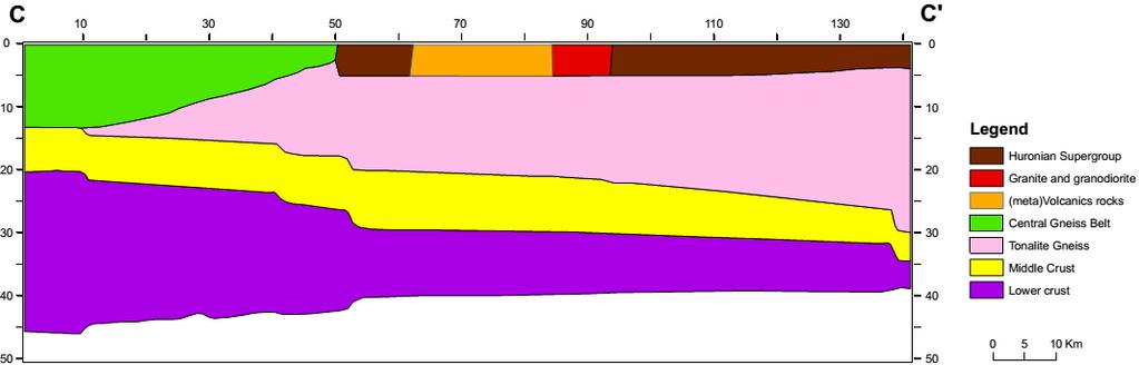
155 141

156 Fig. 5.4: Six schematic E-W and N-S cross sections of the main reservoirs in the region around SNO+ based on the 3-D model. 142

157 Following construction of the 3-D regional crustal model, we divided it into cells of1 km 1 km 0.1 km dimension. The grid has about such cells. Geophysical information for the cells, such as latitude, longitude, depth to the surface, and reservoir type, are to be combined with estimates of the U and Th abundances in each reservoir in order to predict the geoneutrino signal with precise oscillation parameter values. 4. Chemical composition of reservoirs The abundances of U and Th in the seven sub-reservoirs in the upper crust are evaluated from analyses of representative outcrop samples (Appendix A). The OGS has published litho-geochemical databases that provide high quality U and Th abundance data (usually ICP-MS, sometimes INAA) for some of the sub-reservoirs, such as the SIC, the Huronian Supergroup, granitic to granodioritic intrusions, and tonalite/tonalite gneiss. In addition, new unpublished compositional data for glacial tillites in the Huronian Supergroup were provided by Dr. Richard Gaschnig (UMD; personal communication). Data for the Abitibi greenstone belt comes from GEOROC, a web-based geochemical database, which contains a compilation of compositional data for volcanic to metavolcanic rocks from the belt. We use these data to estimate the U and Th abundance of the orange sub-reservoir. This compilation has also been supplemented with OGS data. For the CGB of the Grenville Province, there is limited U data, but abundant Th data provided by Dr. Trond Slagstad (NGU, Norway). The lake sediment is assumed to be sourced by Paleozoic sedimentary rocks. We use the composition of lake sediments in Ontario to represent the composition of the gray unit. The quality of the dataset is improved by excluding all U and Th data determined by XRF. The coordinates and rock types of samples used are matched with the geological 143

158 map. Some sub-reservoirs are further subdivided into more end members according to lithology/composition, such as Abitibi volcanic rock (orange unit), the SIC (blue unit), and felsic intrusions (red unit). The volcanic rocks of the Abitibi greenstone belt are a mixture of felsic, intermediate, and mafic rocks with relative proportions of 5%, 40% and 55%, respectively (Card, 1990). The Main Mass of the SIC is composed of norite (40%), quartz gabbro (10%), and granophyre (50%) (e.g., Lightfoot et al., 1997c). Granite (60%) and granodiorite (40%) are the two dominant types of intrusive rocks that make up the red unit. These proportions are obtained from the geological map by comparing the surface exposure areas of the two rock types in the red unit. For these three subreservoirs, the weighted average composition is obtained using a Monte Carlo simulation (Huang et al., 2013) to predict the geoneutrino signals from these units. After constructing the databases, average U and Th abundances for each of the sub-reservoirs can be evaluated, along with uncertainties. It has long been known that the frequency distributions of the abundances of highly incompatible elements, such as U and Th abundances, in typical crustal reservoirs are strongly skewed and fit a log-normal distribution, rather than a Gaussian distribution (e.g., Ahrens, 1954; Huang et al., 2013). To reduce the influence of rare enriched or depleted samples on the log-normal average, we apply a 1.15-sigma filter that removes about 25% of the data. Then the median value of the distribution is used to represent the central tendency of the distribution, and 1- sigma uncertainty covers 68.3% of the data population. The abundances of U and Th in each sub-reservoir in the regional upper crust are reported in Table 5.5. The U abundances in the pink and green units, which together account for 90% of the upper crustal volume in the 3-D model, are µg/g (ppm) and 2.6 ± 0.4 µg/g 144

159 (ppm), and the Th abundances of these two units are µg/g (ppm) and µg/g (ppm). The number of high quality measurements of U abundances in the CGB gray gneiss is only five, which is the key limitation of the statistics. This is also the reason why the U abundance in the green unit has a symmetric uncertainty. The Wawa-Abitibi sub-provinces are depleted in HPEs, probably due to the fact that the Superior Province is Archean, as Archean crust tend to have lower HPE contents (Taylor and McLennan, 1985). The Huronian Supergroup metasedimentary rocks are the closest unit to the SNO+ detector and are enriched in U ppm and Th ppm relative to the greenstone belt rocks; therefore, this sub-reservoir could be the dominant source of the geoneutrino signal at SNO+. The composition of the middle and lower crust in the 3-D model is inferred from seismic velocity data from the refraction seismic surveys, using the same approach as that adopted by Huang et al. (2013). The seismic velocity in the middle crust is 6.7 ± 0.1 (1- sigma) km/s, and for the top 70% of the lower crust is 7.0 ± 0.2 (1-sigma) km/s while the rest 30% has velocity >7.2 km/s. At room temperature and 600 MPa pressure, felsic amphibolite-facies rocks have an average Vp of 6.34 ± 0.16 (1-sigma) km/s, while the mafic amphibolites have a Vp of 6.98 ± 0.20 km/s. Granulite-facies felsic rocks have an average Vp of 6.52 ± 0.19 km/s, while mafic granulites have an average Vp of 7.21 ± 0.20 km/s. The temperature and pressure correction derivatives are km s -1 C -1 and km s -1 MPa -1 (Rudnick and Fountain, 1995). Assuming a typical conductive geotherm (Pollack and Chapman, 1977) corresponding to a surface heat flow of 50 mw m -2 (the observed average surface heat flow in the Sudbury region (Perry et al., 2009)), the temperature in 145

160 the crust increases linearly to 600 C at 50 km depth. The average depth of middle crust in the regional model is about 25 km, corresponding to a pressure of ~700 MPa and a temperature of ~300 C. Therefore, the pressure-temperature corrected felsic amphibolites have a Vp of 6.25 ± 0.16 km/s and mafic amphibolites have a Vp of 6.89 ± 0.20 km/s. For the lower crust, the pressure is ~1000 MPa and the temperature is ~400 C; therefore, the corrected felsic granulites have 6.45 ± 0.19 km/s and mafic ones have 7.14 ± 0.20 km/s. Given the Vp in middle and top layer of lower crust is set to be 6.7 ± 0.1 km/s and 7.0 ± 0.2 km/s in the model, the fractions of felsic end member in the two reservoirs are 0.3 ± 0.4 and 0.2 ±0.4, which are combined with the compositions of felsic and mafic end members from Huang et al. (2013) to calculate the U and Th abundances in the deep crust. The abundances of U and Th in any single reservoir (except the green unit, as only five data for U abundance are existing) in the regional model are significantly correlated. Table 5.5 reports the correlation between logarithmic values of U and Th abundance in each reservoir. This correlation introduces a non-negligible effect on the uncertainties of geoneutrino signal and radiogenic heat power. Previous reference models (global scale or regional scale) for the geoneutrino signal (e.g., Dye, 2010; Coltorti et al., 2011; Huang et al., 2013) ignored the correlation between U and Th abundances. Here we use Monte Carlo simulation to incorporate fully the variation in U and Th abundances and the influence of the correlation between them in estimating uncertainties. 5. Geoneutrino signal Using the abundances and distributions of U and Th in the 3-D regional crustal model given above, the geoneutrino signal at SNO+ is calculated by summing the 146

161 geoneutrino signal produced by U and Th in each of the cells (see Chapter 2). The geoneutrino production rates from U and Th are and kg -1 s -1, respectively. The oscillated geoneutrino flux at SNO+ from the center of each cell is calculated by taking into account three-flavor survival probability P ee and the geoneutrino energy spectrum (Fiorentini et al., 2012; Fogli et al., 2012). The 1σ uncertainty associated with the survival probability introduces an uncertainty of a few percent to the geoneutrino signal, and is negligible when compared to the other uncertainties (e.g., U abundance). The conversion factor from geoneutrino flux to reported geoneutrino signal is calculated by integrating the geoneutrino energy spectrum and inverse beta decay reaction cross section, and is (TNU cm 2 s) and (TNU cm 2 s) for U and Th, respectively (Fiorentini et al., 2007; Fiorentini et al., 2012). Monte Carlo simulation, as described by Huang et al. (2013), is employed to predict the uncertainty of the geoneutrino signal at SNO+. The uncertainties for thickness and density of each reservoir, correlated abundances of U and Th, and fractions of felsic end members in middle and lower crust are expressed by distributions of generated random number matrices. These input matrices are propagated through the geoneutrino signal calculation to obtain the distribution of the geoneutrino signal. The median value is chosen to describe the central tendency of the skewed output distribution, which is due to the propagation of log-normal distributions of U and Th abundances. The 1-sigma uncertainty covers 68.3% of the population. The predicted geoneutrino signals from U and Th and associated uncertainties (1- sigma) are reported in Table 5.6 for seven sub-reservoirs in the upper crust, middle and lower crust. The uncertainties on the geoneutrino signals are apparently dominated by the 147

162 uncertainties of U and Th abundances. For the upper crust, the Huronian Supergroup is the major geoneutrino source ( TNU; 55% of the total contribution of the upper crust) because of its proximity to SNO+ and its high U and Th abundances. The tonalite/tonalite gneiss in Wawa-Abitibi sub-provinces and CGB gneissic rocks contribute comparable geoneutrino signals (~2 TNU) at SNO+. The felsic intrusions and the SIC both contribute less than 1 TNU. The other two sub-reservoirs (volcanic rocks in Abitibi and Paleozoic sediments) add negligible contributions. The total geoneutrino signal at SNO+ from the regional crust is predicted to be originates from the upper crust. 6. Discussion 6.1. Heat production TNU, 85% of which The estimates of U and Th abundances in different upper crustal sub-reservoirs are based on measurements of outcrops of representative rock types. The heat flow measurements carried out in the Canadian Shield (e.g., Perry et al., 2006) provide a test of the 3-D regional crustal model. We calculate the heat production in each of the reservoirs in the regional crust model (Table 5.6). The heat production and its uncertainty strictly depend on the U and Th abundance. We do not include K in this model, as geoneutrino generated during its decay cannot be detected using current technology. Assuming the K/U in the crust is about 10 4 (e.g., Rudnick and Fountain, 1995; Rudnick and Gao, 2003), the heat production of K is 1/3 of that of U. 148

163 Table 5.5: U and Th abundances in seven sub-reservoirs in the regional upper crust in the 3-D model. UNIT U mean a 1-sigma 1-sigma median n Th mean median n Correlation b PINK all filtered GREEN all filtered Felsic (5%) all filtered ORANGE Intermediate (40%) all filtered Mafic (55%) all filtered GRAY all filtered RED Granite (60%) all filtered Granodiorite (40%) all filtered BROWN all filtered Norite (40%) all filtered BLUE Quartz Gabbro (10%) all filtered Granophyre (50%) all filtered a Log-normal mean, see Huang et al. (2013). b Correlation between logarithmic values of the U and Th abundances 149

164 Table 5.6:Heat production (µw m -3 ) and geoneutrino signal (TNU) at SNO+ from all reservoirs in the 3-D regional model. UNIT Lithology/Geology H(U) H(Th) S(U) S(Th) S(U+Th) PINK Tonalite/Tonalite gneiss (Wawa-Abitibi) GREEN Central Gneiss Belt (Grenville Province) ORANGE (Meta)volcanic rocks (Abitibi sub-province) GRAY Paleozoic sediments RED Granite or granodiorite (Wawa-Abitibi) BROWN Hurionan Supergroup, Sudbury Basin BLUE Sudbury Igneous Complex UC Upper crust MC Middle crust LC Lower crust Total

165 For the Superior Province, the heat production in the upper crust is dominated by the tonalite/tonalite gneiss in the Wawa and Abitibi sub-provinces. From the heat production and the thickness of different reservoirs, we further calculate the heat flow contribution from the crust. The average heat production in the upper crust of the Superior Province is 0.62 µw m -3 (the contributions from U, Th and K are 0.25, 0.29 and 0.08 µw m -3, respectively), with an average thickness of 20.3 km; the middle crust has a heat production of 0.54 µw m -3 and an average thickness of 6.4 km, and the lower crust s heat production is 0.18 µw m -3 and an average thickness is 15.6 km. Therefore, the heat flow contribution from the bulk crust in the Superior Province (Wawa and Abitibi subprovinces region) is 19 mw m -2. If the mantle heat flow in this area is between mw m -2 (e.g., Perry et al., 2006), the average surface heat flow in Superior Province is between mw m -2, which is lower than the measured heat flow of 41 mw m -2 (Perry et al., 2006). However, the uncertainty on the estimate of crustal heat flow contribution is greater than 25% (5 mw m -2 ) or even higher considering the variations of U and Th abundances. Considering uncertainty, the heat flow measurements and the 3-D regional model agree. The upper crust of the CGB of the Grenville Province is relatively enriched in U and Th with a heat production of 1.29 µw m -3 compared to the Superior Province. If the thickness of upper, middle and lower crust in Grenville Province is 14.5, 6.4 and 15.6 km, the crustal contribution to surface heat flow is 25 mw m -2. The Grenville Province also has an average surface heat flow of 41 mw m -2 (Mareschal and Jaupart, 2004). Assuming the mantle heat flow is mw m -2, the total surface heat flow is predicted 151

166 to be mw m -2. Thus, the 3-D regional crustal model predicts a surface heat flow that agrees with surface measurements for the Grenville Province. Heat flow measurements made near the SIC yield an average of 53 mw m -2 (Perry et al., 2009). The locally enhanced heat flow is interpreted as being due to the thick Huronian Supergroup and granitic intrusions that are present around the SIC. The 3- D model has a maximum thickness of Huronian Supergroup to the south of the SIC of 12 km, which can itself contribute a heat flow of 27 mw m -2. If the rest of the upper crust is high-grade gneissic rock such as tonalite gneiss (Lightfoot et al., 1997c), this unit can generate 4 mw m -2. With 6 mw m -2 from deep crust and mw m -2 mantle flow, the surface heat flow near the SIC is calculated to be mw m -2 for the 3-D model presented here. This range agrees with the surface heat flow measurements. However, the 3-D regional model does not have sufficiently high resolution to enable one to determine the variation of surface heat flow in the local area near the SIC due to the lack of dense seismic survey coverage Mantle geoneutrino signal The motivation for undertaking this regional crustal study in the Sudbury area is to determine whether the SNO+ detector, on its own, has the sensitivity to discriminate the mantle geoneutrino signal, which can be obtained by subtracting the crustal signal from future experimentally measured signal (S tot, meas ): S mantle = S tot;meas - S FFC - S LOC. The crustal signal is divided into two components FFC (Far Field Crust) and LOC (LOcal Crust). Huang et al. (2013) predicted the FFC signal at SNO+ to be LOC to be TNU TNU and the 152

167 5.3 Our regional crustal study predicts an updated LOC signal of TNU, which is within 1-sigma uncertainty of the prediction obtained by using the global reference model. The uncertainty for the LOC signal from the regional crustal study is larger than the uncertainty from the global reference model. The main reason for the larger uncertainty is the large variations in U and Th abundances in each sub-reservoir, especially the Huronian Supergroup, of the upper crust (Table 5.5). The only exception is the SIC, for which only a single dataset from an OGS Open File Report 5959 (Lightfoot et al., 1997a) is used to estimate the U and Th abundance. Considering the much larger surface exposures of other sub-reservoirs, the variations of rock type and chemical composition become larger. The bulk crustal geoneutrino signal at SNO+ is estimated to be TNU, by summing the FFC signal (Huang et al., 2013) with LOC signal from this study. This regional crustal study for Sudbury slightly reduces the uncertainty on the predicted bulk crustal geoneutrino signal compared to the prediction based on global reference model (Chapter 3; Huang et al., 2013), which is TNU. The continental lithospheric mantle is predicted to produce about 2 TNU at SNO+ (Huang et al., 2013). Assuming a BSE compositional model of McDonough and Sun (1995), the predicted mantle signal at SNO+ is 7 TNU (Šrámek et al., 2013). Without taking into account the uncertainties on the signal from continental lithospheric mantle and convecting mantle, the total geoneutrino signal at SNO+ is predicted to be TNU. 4 For the sake of simplicity, we adopt an uncertainty on the bulk crustal signal at SNO+ as 5.1 TNU in the discussion below. Following the equations defined by Dye (2010), the mantle signal determination at SNO+ has a systematic uncertainty of

168 TNU, assuming the systematic uncertainty for nuclear reactor events is 0.9 TNU and for detection exposure determination is 1.9 TNU. The counting uncertainty for geoneutrino detection decreases with accumulation of geoneutrino events, following Poisson s law. Assuming SNO+ can see 30 geoneutrino events per year, the counting uncertainty to geoneutrino detection rate drops to 11% of 40 TNU after three years. By summing the counting and systematic uncertainty for the geoneutrino event rate at SNO+, the total uncertainty of 4.7 TNU. Therefore, the mantle signal determination at SNO+ has a total uncertainty of 6.9 TNU after three years of full operation after subtracting the crustal signal from the measured total signal. Šrámek et al. (2013) predicted the mantle geoneutrino signal at SNO+ using different BSE compositional models and mantle structure to range between 2 to 16 TNU. To resolve these different mantle signals, the uncertainty for determining the mantle signal should be, at most, 7 TNU, which is the same as SNO+ s sensitivity to the mantle signal as described above. Unfortunately, the current constraints on the abundances and distributions of U and Th in the regional crust, especially in the Huronian Supergroup, are not good enough to make this goal feasible. There are three possible ways to change this situation: 1) improve our knowledge of the distribution of the Huronian Supergroup by undertaking higher density seismic surveys, as well as performing a systematic study of the U and Th abundances in different representative metasedimentary/sedimentary rocks; 2) combing the experimental results at the three operating detectors to determine the mantle signal, rather than relying on any single detector; 3) conducting a geoneutrino experiment, such as the proposed Hanohano detector (Learned et al., 2008), which is carried out in the oceans in order to minimize the signal from continental crust. 154

169 Performing high density seismic surveys within the Huronian Supergroup would allow better estimation of its physical structure with smaller uncertainty (~10 %). The geophysical uncertainty will contribute ~±1 TNU on the geoneutrino signal originating from the Huronian Supergroup. The relatively large variations of U and Th abundances in the Huronian Supergroup are the dominant source of uncertainty on the geoneutrino signal from this sub-reservoir. Ideally, detailed geochemical mapping of U and Th abundance variations in the area will improve the geoneutrino signal prediction significantly. If the geochemical uncertainties on the Huronian Supergroup (e.g., U and Th abundances) can be reduced to 10 to 20 %, they would contribute ~±1 to ±2 TNU uncertainty on the geoneutrino signal. Combining the geophysical and geochemical uncertainty contributions, higher resolution studies of the Huronian Supergroup is likely to reduce the uncertainty on the geoneutrino signal from this reservoir to ~±2 TNU, + smaller than the TNU obtained in this study. Given that this task is feasible in the near future, the LOC geoneutrino signal at SNO+ could have a reduced uncertainty of ~±2.5 TNU, and the bulk crust signal would have an uncertainty ~±3 TNU. Following this approach, the extracted mantle signal from future experimental results at SNO+ will have an uncertainty ~±5.6 TNU, which would allow better resolution of the various BSE compositional models. 7. Conclusions We have constructed a 3-D regional crustal reference model aimed at predicting the geoneutrino signal at SNO+, the third geoneutrino detector located in Sudbury, Ontario, Canada, which is scheduled to come on-line in The uncertainty of the predicted geoneutrino signal is estimated through Monte Carlo simulation, and stems 155

170 mainly from the large uncertainties on U and Th abundances in the upper crust. The main results reached in this study are as follows: 1. Surface geological map, refraction and reflection seismic surveys, receiver function analyses, and interpreted vertical crustal cross sections in the Sudbury region are integrated to a 3-D model for the six 2 2 tiles centered at SNO+. The average thickness of the regional crust is estimated to be 42.3 ± 2.6 km, which is in good agreement with the results obtained in the previous global crustal reference model (Huang et al., 2013). The thickness of upper crust reaches 20.3 ± 1.1 km, which accounts for about half of the bulk regional crust. 2. The upper crust is subdivided into seven sub-reservoirs in order to increase the resolution for predicting the geoneutrino signal. The tonalite/tonalite gneiss in the Wawa and Abitibi sub-provinces is the dominant rock type (60% of upper crust), and it has µg/g U and µg/g Th. The depletion of HPEs relative to global average upper continental crust is probably due to the fact that Superior Province is a remnant of an Archean continent. The high grade gnessic rock, with 2.6 ± 0.4 µg/g U and µg/g Th, in the Central Gneiss Belt (CGB) of Grenville Province is the second dominant rock type in the 3-D model (30% of upper crust). The Huronian Supergroup metasedimentary rocks are the closest unit to the SNO+ detector and are enriched in U µg/g and Th µg/g relative to the other units. All of the uncertainties are propagated through Monte Carlo simulation to the geoneutrino signal prediction. 156

171 3. The total regional crust contribution of the geoneutrino signal at SNO+ is predicted to be TNU. This signal is somewhat lower than the prediction made using the global reference model (Huang et al., 2013), which is TNU. This difference is likely to be due to the lower HPEs in Archean to Proterzoic rocks of the Canadian Shield relative to the global average bulk upper continental crust. Considering the uncertainty, the two predictions of geoneutrino signal are consistent with each other. The Huronian Supergroup is predicted to be the dominant source of the geoneutrino signal and its uncertainty at SNO+. The natural variation in U and Th abundances within the Huronian Supergroup is the primary source of the large uncertainty on the predicted geoneutrino signal. 4. Assuming that the continental lithospheric mantle and convecting mantle together contribute 9 TNU signal to SNO+, the total geoneutrino signal at SNO+ is estimated to be TNU The large uncertainty in the crustal geoneutrino signal indicates that SNO+, on its own, is unlikely to provide sensitivity to the mantle geoneutrino signal, and therefore the debate regarding BSE compositional models. Several future approaches to improve the determination of mantle geoneutrino signal are: improving the 3-D regional model for predicting the regional crustal contribution by increasing the resolution of the distribution of the Huronian Supergroup with a higher density of local seismic surveys and geochemical analyses; combining experimental results at the three operating detectors to place better constraints on the mantle signal; and conducting geoneutrino 157

172 detection in the oceans, such as the proposed Hanohano detector, in order to minimize the crustal signal. 158

173 Chapter 6: Summary and future work Detection of geoneutrinos provides the possibility to constrain the total radiogenic heat power in the Earth and distinguish between different Bulk Silicate Earth (BSE) compositional models by comparing the experimental results with model predictions (Fig. 6.1). The SNO+ detector, located in Sudbury, Canada, will degin counting geoneutrino events from To interpret the measured geoneutrino signal at SNO+, we constructed both a global and a regional scale reference model to predict the geoneutrino signal at this site. The global reference model presents a spatially refined crustal reference state of the deep continental crust by coupling seismic velocity data with bulk compositional data (i.e., SiO 2 content) for amphibolite and granulite facies rocks, and from this relationship (i.e., SiO 2 vs. Vp) determining a geospatial 3-D estimate, with uncertainties, of the crustal U and Th contents. The goal of the SNO+ specific regional crustal study (which focuses on six 2 2 tiles centered at SNO+) is to improve the estimate of the uncertainty of geoneutrino signal from the local crust, which can be subtracted from the experimentally measured total signal at SNO+ to estimate the mantle geoneutrino signal. The main conclusions drawn from this dissertation are: 1. The total geoneutrino signal at SNO+ is predicted to be the sum of the regional crustal signal ( TNU, which is TNU) from the regional reference model, the far field crust signal ( TNU) from the global reference model, 2 TNU from continental lithospheric mantle, and 7 TNU from the convecting mantle that has an assumed BSE composition of that

174 reported in McDonough and Sun (1995). The uncertainties are only precisely determined for the crustal signal. 2. The continental crust is the dominant geoneutrino source, as it contributes ~75 % of the total geoneutrino signal at SNO+. This reservoir produces TW of radiogenic heat, approximately one third of the total radiogenic power in the Earth assuming a model that has 20 ng/g of U, Th/U of 3.9 and K/U of ~10 4 (McDonough and Sun, 1995). 3. The asymmetric uncertainties on the predicted geoneutrino signal and radiogenic heat power are due to the log-normal distributions of U and Th in the crust. Monte Carlo simulation was employed to incorporate all sources of uncertainties. In both the global and regional reference models, the large variations in U and Th abundances are the dominant source of uncertainty on the predicted geoneutrino signal at SNO+. 4. Different BSE compositional models produce variable radiogenic heat power, ranging from 10 TW to 30 TW, with the geoneutrino signal at SNO+ ranging from 2 to 16 TNU. The uncertainty of the experimentally determined mantle geoneutrino signal at SNO+ will be about 7 TNU after three years of full operation, which is not enough to delineate permissible BSE compositional models. Although this dissertation does not positively support the hypothesis that SNO+ will, after several years of counting, be capable of providing geoneutrino data needed to delineate the different BSE compositional models, additional studies can be carried out in order to understand how geoneutrino measurements can benefit geoscience. Three main 160

175 further study directions will serve to enhance our effort to determine the mantle geoneutrino signal and are described as below. The uncertainty on the geoneutrino signal at SNO+ produced in the continental crust can be better characterized by improving both the global and regional reference models. The global reference model predicts the geoneutrino signal by using the average upper continental crustal composition of Rudnick and Gao (2003) and assumes that the U and Th abundances are independent from each other in a single reservoir. Refinement of the upper continental crustal compositional model can be had from compiling chemical composition datasets for shale, graywacke, loess and tillite samples, all of which are likely to provide an the average for the upper continental crust of their respective provenances. The well documented correlation between U and Th abundances in rocks must be incorporated into the geoneutrino signal calculation, which has not been done in any of the previous global reference models. The most updated global crustal model, CRUST 1.0, by Laske et al. (2013) can also be implemented in the reference model described in Chapter 3. This higher resolution global crustal model incorporates more seismic data and should be an improvement over the older CRUST 2.0. From the regional crust study, we know that the Huronian Supergroup, the closest unit to SNO+, is the dominant source of geoneutrinos (and also the uncertainty) at the detector. Conducting additional seismic surveys, coupled with additional geochemical analyses of representative samples having a higher sample density in the local area (e.g., 50 km by 50 km) within the Huronian Supergroup should improve the resolution of the regional reference model and determination of the uncertainty on regional crustal geoneutrino 161

176 signal. Further reducing the uncertainty on the regional crustal signal by ~2 TNU will allow the determination of the mantle geoneutrino signal at SNO+. All the three geoneutrino detectors are located in continental crust, which acts as a significant background for the mantle geoneutrino signal. It is difficult for any single detector to accumulate significant amount of geoneutrino events to refine the mantle signal. However, combined analyses of experimental results at the different locations can provide joint constraints on the mantle signal (Fiorentini et al., 2012). The ideal location to measure a mantle geoneutrino signal is in the oceans, where the contribution from continental crust is reduced by more than an order of magnitude. The proposed 10 kiloton scale Hanohano experiment, which could be carried out in the Pacific Ocean, will receive less than 3 TNU signal (~25% of the total signal) from the bulk crust, which will make the direct measurement of the mantle geoneutrino signal feasible. 162

177 Fig. 6.1: Comparison between experimental geoneutrino results and model predictions at KamLAND and Borexino sites. Red dots and blue squares are the experimentally determined geoneutrino signals at KamLAND and Borexino, respectively (Araki et al., 2005; Bellini et al., 2010; Gando et al., 2011; Bellini et al., 2013; Gando et al., 2013). The associated uncertainties are 1-sigma. Dark brown represents the near field crustal geoneutrino signal (LOC signal) determined by local crust studies (Enomoto et al., 2007; Coltorti et al., 2011); light brown represents the far field crustal geoneutrino signal (FFC) based on the global reference model of Huang et al. (2013). Different BSE compositional models yield variable geoneutrino signals from the mantle (various green colors). Considering the uncertainty associated with geoneutrino detection, neither detector can now distinguish different BSE models at the 1-sigma confidence level. 163