NUMERICAL MODELLING OF LANDSLIDE RUNOUT A continuum mechanics approach

Transcription

1 Marina Pirulli NUMERICAL MODELLING OF LANDSLIDE RUNOUT A continuum mechanics approach Ph.D. Degree in Geotechnical Engineering POLITECNICO DI TORINO Department of Structural and Geotechnical Engineering

2 Front cover: The rock avalanche of Goldau, 1806 (Switzerland)

3 POLITECNICO DI TORINO Department of Structural and Geotechnical Engineering NUMERICAL MODELLING OF LANDSLIDE RUNOUT A continuum mechanics approach Ph. D. Degree in Geotechnical Engineering (17 th Cycle) April 2005 Author Marina Pirulli Supervisor Prof. Claudio Scavia Co-Supervisors Prof. Oldrich Hungr Dr. Anne Mangeney Politecnico di Torino University of British Columbia Institut de Physique du Globe de Paris Head of the Ph.D. Programme in Geotechnical Engineering Prof. Renato Lancellotta Politecnico di Torino Board of Examiners Prof. Leonardo Cascini Prof. Renato Ribacchi Prof. Luigi Sambuelli Università di Salerno Università di Roma La Sapienza Politecnico di Torino

4

5 Qual è quella ruina che nel fianco di qua da Trento l Adice percosse, o per tremoto o per sostegno manco, che da cima del monte, onde si mosse, al piano è sì la roccia discoscesa, ch alcuna via darebbe a chi sù fosse (da Divina Commedia Inferno Canto XII, Dante Alighieri)

6

7 I wish to express special thanks to Prof. Claudio Scavia, who has always pushed me to go ahead and has always restored the right determination in me when problems look insurmountable and preliminary results disappointing. Please excuse me for whenever I interrupted your work with my doubts, but each discussion has been very precious. Three years ago we had a common purpose; it has not been easy but I think that many goals have been attained. On the 28th of January 2002, km away from Torino, I met Prof. Oldrich Hungr for the first time. His infinite experience and his precious suggestions have helped me to better know and understand how to face the problems that I have worked on. I feel gratitude not only for all his help but also for having introduced me to the wonderful world of the opera. Scott McDougall has given me the opportunity to work on some of the cases that he has also analysed. I have greatly appreciated all his help. An important turning point in my work was due to Prof. Renato Lancellotta. Thanks to him, I had the opportunity to meet Prof. Kolumban Hutter, whose complex continuum mechanical theory induced me to pass many sleepless nights but helped me to attain some fundamental results. Prof. Hutter gave me the opportunity to visit the Institut de Physique du Globe de Paris, where Dr. Anne Mangeney put their code at my disposal. She followed my progress day by day with deep interest. She helped me not only to understand the source code but also to solve some of the neverending problems. I also wish to thank Dr. Marie-Odile Bristeau, whose detailed knowledge of each routine in the code helped me solve some fundamental problems. In Paris I had the opportunity to compare my knowledge and my education as an engineer to those of mathematicians and physicians; to my great satisfaction this synergy has produced good results. The experience of a geologist has also been necessary. I thank Dr. Ferruccio Forlati, who has given a few precious hints on how to deal with some topics. To all the members of my family, a warm embrace for having always supported my decisions, even when these took me away from home. I cannot forget any of my friends from Condove, Cels and Rivoli. Special thoughts go to: Roberta, the best friend that can be desired; Massi, who promptly came to my aid when I was quarrelling with the computer and put a whole staff of experts on informatics at my disposal; Andrea, Danilo XL, Gian, Marcello, Marco, Ombri, Roberto and Sabrina.

8

9 Contents Chapter 1 Introduction Chapter 2 Landslide classifications and rock avalanche features Introduction Landslide classifications To understand each other Rock avalanche Avalanche dynamics Entrainment of substrate material Excessive mobility of rock avalanches Chapter 3 Run out models of rock slope failure Introduction Experimental approach Empirical approach Analytical approach Lumped mass Continuum mechanics Kinetic theory Discontinuum mechanics Dynamic equations of equilibrium Contact law

10 Chapter 4 Continuum mechanics approach: DAN and SHWCIN codes, theoretical aspects Introduction Field equations Reference frame Rheological constitutive laws The three-dimensional model, SHWCIN Approximation Numerical Model Finite Volume Method Kinetic formulation Friction The two-dimensional model, DAN Numerical model The flow resistance term, T The pressure term, P Chapter 5 From SHWCIN to RASH 3D. Numerical model upgrade Introduction Structured vs. Unstructured Original vs. modified version of the Code Gravitational acceleration effects Original vs. modified version of the Code Validation Earth pressure coefficients Theoretical analysis Original vs. modified version of the Code Validation and observations Rheology Theorical analysis Original vs. modified version of the Code Pore water pressure Original vs. modified version of the Code Validation of the final version of RASH 3D Deflected run out experiment Frank slide (Canada) Six des Eaux Froides (Switzerland)

11 Contents Chapter 6 DAN. Back analyses of case histories Introduction Collection and cataloguing of case histories General characteristics Back analysis procedure Validation of the coupled methodology Results of back analyses Observations Chapter 7 Conclusions and further developments Appendix A Analysed case histories... I Avalanche Creek... I Avalanche Lake... IV Charmonetier... VII Claps de Luc... IX Conturrana... XI Dusty Creek... XIII Eagle Pass... XV Elm... XVII Felik... XIX Flims (1939)... XXI Flims Pleistocene... XXIII La Madeleine... XXV Mt. Ontake... XXVII Nomash River... XXX Pandemonium Creek... XXXII Rubble Creek... XXXV Scanno... XXXVII Six des Eaux Froides... XL Vajont... XLII Val Pola... XLV Appendix B Earth pressure coefficients... XLVII Bibliography... XLIX

12

13 Chapter 1 Introduction p Increasing population density and development of mountainous terrains bring human settlements within reach of landslide hazards. Perhaps the most serious threat arises from small, high frequency landslides such as debris flows and debris avalanches. On the other hand, large and relatively rare rock avalanches also constitute a significant hazard, due to their prodigious capacity for destruction. Such landslides involve the spontaneous failure of entire mountain slopes, involving volumes measured in tens or hundreds million m 3 and travel distances of several kilometres. Stability analysis of entire mountain slopes is exceedingly difficult. Thus, concern about the possible occurrence of a rock avalanche usually arises only once certain precursory signs of impending failure appear. When such signs are identified, monitoring of displacements, strains, piezometric pressures or rock noise can be used to gauge deterioration in stability and signal the onset of failure (e.g. Schuster and Krizek, 1978). Flow-like movements of rocks can then be identified among the most dangerous and damaging of all landslide phenomena. Since it often proves impossible to mitigate their destructive potential by stabilising the area of origin, risk analyses, including predictions of runout, have to be performed. With these predictions losses can be reduced, as they provide means to define the hazardous areas, estimate the intensity of the hazard (which will serve as input for risk studies), and work out the parameters for the identification of appropriate protective measures. At the same time, reliable predictions of runout can help to avoid exceedingly conservative decisions regarding the development of hazardous areas.

14 1.2 Risk evaluation of these events requires the comprehension of two fundamental problems: the initiation and the runout. Even though the specification of the initial conditions is also a primarily problem, which is not yet resolved, the runout, that is the flowing and stopping phases of the mass, is here analysed. Numerical simulation should provide a useful tool for investigating, within realistic geological contexts, the dynamics of these flows and of their arrest phase. In the 1970 s the most widely used and perhaps earliest model proposed for the analysis of rockslides and similar phenomena was that of a rigid block on an inclined plane (e.g. Koerner 1976, McLellan and Kaiser 1984, Huchinson 1986, Sassa 1988). Few laboratory experiments were then done, but first qualitative and quantitative observations on the obtained results became fundamental for a better understanding of movement runout behaviour and motivated the introduction of more and more sophisticated apparatus. In recent years lumped mass models have been shelved. Simple empirical correlations among historical data (e.g. Scheidegger 1973, Hsu 1975, Li 1983, Davies 1982, Nicoletti and Sorriso Valvo 1991) have then been put beside new and more sophisticated models based on a continuum mechanics approach (e.g. Hungr 1995, Chen and Lee 2000, Denlinger and Iverson 2004). Together with continuum mechanics models, a noteworthy type of modelling is that based on a discontinuum mechanics approach (e.g. Strack and Cundall 1984, Cundall 1988, Walton et al. 1988, Will and Konietzky 1998), in which the run out mass is modelled as an assembly of particles moving down along a surface. Nowadays this last approach still presents some macroscopic limitations that in some way compromise a satisfactory application to large movement analysis. It is probably fair to state that Savage and Hutter in 1989 developed the first continuum mechanical theory capable of describing the evolving geometry of a finite mass of a granular material and the associated velocity distribution as an avalanche slides down inclined surfaces. Their model provided a more complete analysis of such flows than previous models had done, and its extension as well as comparison with laboratory experiments demonstrated it to be largely successful. A continuum mechanics approach assumes that during an avalanche, the characteristic length in the flowing direction is generally much larger than the vertical one, e.g. the avalanche thickness. Such a long-wave scaling argument has been widely used in derivation of continuum flow models. This leads to depth-averaged models governed by generalized Saint Venant equations. Nowadays, these models provide a fruitful tool for investigating the dynamics and extent of avalanches. Anyway, whatever the applied analytical model, results of a numerical simulation depend on the value assigned to the constitutive parameter of the assumed rheology.

15 Chapter 1: Introduction 1.3 The aim of the dissertation is the development and validation of a three dimensional numerical model able to run analyses of propagation on a complex topography and the setting of a procedure direct to define some reference values for characteristic parameters of an assumed rheology. Case histories having a different runout path and material type are analysed and compared, the obtained values could be considered useful guidelines to study a potential landslide (before the event). The choice of a certain approach rather than another is the result of a careful analysis of advantages and disadvantages of each existing method. All choices are made never forgetting to remain focused on real problems and real behaviour of a mass. By consequence, each problem tackled and solved is directed to guarantee more realistic results. Whatever the chosen numerical approach, it is fundamental to know in detail the type of phenomenon that will be studied. In this sense, it is important to learn from past events and to always have on mind that each analysed problem is not abstract but it is linked to a real site. In the present work, a continuum mechanics approach has been followed. The original version (SHWCIN) of the implemented three dimensional code was developed at the Institut de Physique du Globe de Paris but before using it to run analysis of propagation on a complex topography many fundamental changes are necessary. Trying to reduce the uncertainty range of values to be assigned in prediction to rheological parameters, the numerical code DAN (Hungr, 1995) is applied to back analyse a set of case histories of landslides selected from literature. For prediction, the main limitation of DAN is due to the fact that it reduces a complex and heterogeneous three dimensional problem into an extremely simple formulation and the width of propagation is a part of the input data. But, when a back analysis is run, the geometry of propagation is already known. Therefore, the limits of DAN in some way disappear. Also, cases for which a DEM (Digital Elevation Model) is not available can be analysed. Moreover, advantages in using this code are mainly due to its simplicity, it makes possible an immediate and rapid numerical simulation of many real cases. It also allows the choice among different rheologies, some of which are particularly simple, reducing the number of mechanical parameters that have to be defined. The methodology here proposed consists in using DAN to run back analyses of as many case histories as possible and the new three dimensional code to predict propagation of a mass on a complex topography. It is important to underline that when values obtained from back analyses are used to simulate a potential landslide, only cases having similar characteristics (e.g. run out area shape, material type, glacier along the path) can be compared.

16 1.4 To guarantee correctness of this approach it is necessary to verify that DAN results, if used as input data in a three dimensional numerical code, give approximately the same solution. Cases for which a DEM pre-collapse is available are analysed with both DAN and the new code. After a critic overview of landslide classifications and a detailed description of those phenomena known as rock avalanches (Chapter 2), a description of existing propagation methods has been done, underlining advantages and disadvantages of each considered approach (Chapter 3). On the basis of possibility of application on analysis of real cases a continuum mechanics approach has then been followed, two numerical codes have been analysed: SHWCIN and DAN (Chapter 4). The SHWCIN code was originally used to carry out simple numerical simulations of a mass released from a gate or from a hemi-spherical cap on an inclined plane and results were analysed considering the centre line section. To simulate the movement on a complex three dimensional topography, the code has been numerically implemented allowing to: reduce mesh-dependency effects on results of propagation by using an irregular mesh, change gravity components as a function of the considered topography, change earth pressure coefficients in a condition of anisotropy of normal stresses, take into account both different constitutive laws and pore water effects. Each of these changes has been carefully validated. Once the final version of the code was obtained it has been tested through numerical analysis of laboratory tests and back analysis of case histories obtained from literature (Chapter 5). In order to create a database of well described phenomena and rheological parameters, that can be useful guidelines when prediction is the aim of an analysis, case histories have been analysed with DAN following a procedure that gives the possibility of calibrating the model in order to obtain the best value for each of the parameters required by the assumed rheology (Chapter 6).

17 Chapter 2 Landslide classifications and rock avalanche features 2.1 Introduction As a result of the widespread use of the landslide classifications, certain terms describing common types of mass movements have become entrenched in the language of engineering geology. The landslide classifications of Varnes (1954, 1978) and Hutchinson (1968, 1988) are today the most widely accepted systems. Nevertheless, literature on engineering geology of landslides continues to be plagued by inconsistent terminology and ambiguous definitions of various landslides types. In this frame fundamental is the work performed by Hungr et al. in 2001, in which an effort is made in giving a more precise definition of the used terms. The aim is to guarantee the preservation of the original meaning of each term and to make the application less ambiguous. Phenomena such as as rock avalanches are rare but are considered among the most destructive and dangerous natural calamities. Catastrophic failures at a given site are difficult to estimate. Thus, concern about the possible occurrence of a rock avalanche usually arises only once certain precursory signs of impending failure appear. The frequency of occurrence and amplitudes of these disastrous events appear to have increased in recent years, possibly due to increase in land use and development activities, anticipated warming of the Earth s atmosphere, the associated increase of extreme storms, poor forestry practices and land misuse in the mountainous areas. This implies an increase in damage of properties and infra-structures and a further endangering of public life.

18 2.2 Reliable methods for the prevention and/or reduction of the effects of such disasters are therefore in great need. Evidently, concerned authorities who are responsible for the planning and development in these regions have considerable interest in it and these justify a more detailed analysis of rock avalanches phenomena. 2.2 Landslide classifications The term landslide denotes the movement of a mass of rock, debris or earth down a slope (Cruden, 1991). The phenomena described as landslides are not limited either to the land or to sliding, the word has a much more extensive meaning than its component parts suggest. Phenomena like falls, topples, slides, spreads and flows (Figure 2.1) are encompassed. Figura 2.1. Slope movement types

19 Chapter 2: Landslide classifications and rock avalanche features 2.3 Landslides can be initiated by rainfall, earthquakes, volcanic activity, changes in groundwater, disturbance and change of a slope by man-made construction activities, or any combination of these factors. Landslides can also occur underwater, causing tidal waves and damage to coastal areas. These types of events are called submarine landslides. The most widely accepted landslide classifications are by Hutchinson (1968) and by Varnes (1978). Both classifications are based on earlier systems (Sharpe, 1938) and have tended to converge over recent years, particularly in terminology. The synthesis of these two classifications has continued. Huchinson (1988) springs from Hutchinson (1968) and Skempton and Hutchinson (1969) and draws heavily on the work of others, particularly that of Varnes (1978). The suggested classification pays regard primarily to the morphology of slope movements, with some consideration being given also to mechanism, material and rate of movement. It is primarily applied to sub-aerial mass movements, on natural or man-made slopes. It excludes the very large-scale movements involved in gravity tectonics, mass movements involving subsidence and other forms of sinking of the ground surface, all mass transport phenomena and avalanches of snow or ice. The criteria used in the classification of landslides presented by Cruden and Varnes (1996) follow Varnes (1978) in presuming the knowledge of movement mechanisms and emphasizing type of movement and type of material (Table 2.1). TYPE OF MOVEMENT Falls Topples Slides Spreads Flows Complex TYPE OF MATERIAL Rock Debris (coarse soil) Rotational Earth (fine soil) Translational Table 2.1. Slope movement classification after Varnes (1978) Any landslide can be then classified and described by two nouns: the first describes the material and the second describes the type of movement (e.g. rock fall, debris flow). In Cruden and Varnes (1996) the names for the types of material are unchanged from Varnes classification (1978): rock (a hard or firm mass that was intact and in its natural place before the initiation of movement), earth (describes material in which 80 percent or more of the particles are smaller than 2 mm) and debris (contains a significant proportion of coarse material, 20 to 80 percent of the particles are larger than 2 mm and the remainder are less than 2 mm). Movements have again been

20 2.4 divided into five types: falls, topples, slides, spreads and flows. The sixth type proposed by Varnes (1978), complex landslides, has been dropped from the formal classification, although the term complex has been retained as a description of the style of activity of a landslide indicating the sequence of movement in the landslide and distinguishes this landslide from a composite one, in which different movements occur simultaneously on different parts of the displaced mass (Table 2.2). ACTIVITY STATE (what is known about the timing of movements) DISTRIBUTION (where the landslide is moving) Active Advancing Complex Reactivated Retrogressive Composite Suspended Widening Multiple Inactive Enlarging Successive Dormant Confined Single Abandoned Diminishing Stabilized Moving Relict STYLE (the manner in which different movements contribute to the landslide) DESCRIPTION OF MOVEMENT RATE WATER CONTENT MATERIAL TYPE Extremely rapid Dry Rock Fall Very rapid Moist Earth Topple Rapid Wet Debris Slide Moderate Very wet Spread Slow Flow Very slow Extremely slow Table 2.2. Slope movement classification after Cruden and Varnes (1996) The name of a landslide can become more elaborate as more information about the movement becomes available. To build up the complete identification of the movement, descriptions are added in front of the two-noun classification using a preferred sequence of terms. The suggested sequence provides a progressive narrowing of the focus of the descriptors, first by time and then by spatial location, beginning with a view of the whole landslide, continuing with parts of the movement, and finally defining the materials involved. The recommended sequence describes

21 Chapter 2: Landslide classifications and rock avalanche features 2.5 activity (including state, distribution, and style) followed by descriptions of all movements (including rate, water content, material, and type). For instance, the very large and rapid slope movement that occurred near the town of Frank, Alberta, Canada, in 1903 (McConnell and Brock, 1904) was a complex, extremely rapid, dry rock fall-debris flow (Figure 2.2). Figura 2.2. Frank slide, 1903 Alberta (Canada). 2.3 To understand each other Landslides exhibit an initial failure stage followed by a runout. A central problem in classification is what weight to give to each of these two, often contrasting stages. In Varnes classification a complex landslide is described considering that the type of movement and the type of material change as it progresses. A landslide is then described at the beginning of each successive phase (i.e. rock fall-debris flow). Unlike Varnes, Hutchinson s classification appears to be related more closely to the conditions of failure (Crozier, 1986). A classification system can be taxonomic, employing a hierarchy of descriptors to form a branching structure. Alternatively, it can be a filing system, which places items into classes on the basis of various attributes. Hutchinson s classification is essentially non-taxonomic, Varnes classification is weakly taxonomic.

22 2.6 The different approach followed by the two considered classifications can be well emphasized if the status of flow is considered. In the scheme of Varnes (1978) the mechanism of the movement assumes a fundamental value. Following this approach, all slope movements involving significant internal distortion of a moving mass would be classed as flows. Morphology is the principal factor in Hutchinson s classification; phenomena with different mechanism are classed together as a function of their overall behaviour. From this point of view, mudslides, flowslides, debris flows, and sturzstroms (rock avalanches) are all defined flow-like movements, and any commitment to a specific kinematic model is avoided. In a way Varnes scheme is perhaps easier to apply and requires less expertise to use, Hutchinson s classification has particular appeal to the engineer contemplating stability analysis. On the other way, it is sometimes difficult to easily estimate aspects like the average grain-size distribution of a deposit, because of lateral and vertical nonhomogeneity of many landslides together with the possibility that a poorly-sorted material can be fully supported by a clayey matrix with high coarse-grain content. The term flow itself can induce a lack of understanding. Which is the real difference between a slide and a flow? The definition of slide by the Oxford Concise Dictionary, is progress along smooth surface with continuous friction on the same part of object progressing. The very fact that a rigid block was converted into a debris tongue should be sufficient argument that the fallen block did not simply slide; there was not a continuous friction on the same part of object progressing; instead, more and more new surfaces on freshly broken debris came into contact with the valley floor. In contrast, flow has been defined as glide along a stream. The mass moulded itself to fit the geometry of the valley floor and glided along as a debris stream, is thus not a slide but a flow. A second question originates if the difference between fall and flow is considered. Heim (1932) describes the movement of Elm (Switzwerland, 1881) as a large mass broken into thousand pieces, falling at the same time along the same course, whose debris had to flow as a single stream. The uppermost block at the very rear of the stream would attempt to get ahead. It hurried but struck the block slightly ahead, which was in the way. Cruden and Varnes (1996) define fall a material that descends by falling, bouncing, or rolling. Explanatory is the definition introduced by Sander (1948) where a flow is described as a continuously arranged relative movement, carried out by sufficiently small (compared to the system under consideration) parts. The type of movements does not only depend on the materials in which it takes place, but also on the scale of the movement.

23 Chapter 2: Landslide classifications and rock avalanche features 2.7 In accordance with this consideration the landslide classification introduced by Rochet (1987) assumes the volume as the parameter that allows the organization of the movements as a function of the system under consideration. But the interpretation of the attribute sufficiently small is left to everyone personal discretion. As a result of the widespread use of the landslide classifications certain terms describing mass movements have become entrenched in the language of engineering geology. Since conservativism is a very important attribute of classification and language is to be an effective communication tool, Hungr et al. (2001) explore the three taxonomic dimensions (movement mechanism, material type and velocity of movement) as used in Varnes classification in order to review the main characteristics of flows-type movements as defined by Hutchinson. Fundamental in Hungr s work is the attempt of making a translation matrix between the terms used in Varnes classification and those contained in Hutchinson s classification (Table 2.3). If attention is focused on Table 2.3 a new doubt can be aroused by the presence of phenomena like debris avalanche and rock avalanche. A rock avalanche is usually defined as an extremely rapid flow of dry debris (Hsu, 1975). The presence of the ambiguous term debris avalanche is clarified if a detailed analysis of the existing classifications is run. A debris avalanche originates in debris and the movement is assumed as partly or fully saturated, while a rock avalanche originates in rock and is mainly dry (Hungr et al., 2001). VARNES (1978) HUTCHINSON (1988) HUNGR et al. (2001) Wet sand, silt flow Flow slide Sand, silt flow slide Rapid earth flow Flow slide (clay) Clay flow slide Loess flow Flow slide (loess) Loess flow slide Dry sand flow - Dry sand slide Earth flow Mudslide Earth flow - Mudflow Mud flow Debris avalanche Hillslope debris flow Debris avalanche Debris flow Debris flow Debris flow - Hyperconcentrated flow Debris flood Rock avalanche Sturzstrom Rock avalanche Table 2.3. Translation matrix for landslides of the flow type after Hungr et al. (2001). A universal classification does not exist. All the existing classifications can generate doubts both in terminology and in attributes to be assigned to each type of movement, especially if the analysis is carried out by a non-expert. A text-book case is difficult to be found, the influence of geological and topographic conditions very

24 2.8 frequently cause the real phenomenon to be a combination of two or more types produced either in a simultaneous process or in successive and interconnected processes. Fundamental is to have a huge and clear knowledge of the possible behaviour that a mass can assume, knowledge that can be enriched through field trips and analyses of as many case histories as possible. Once that familiarity is attained, analysis of existing classifications becomes easier. 2.4 Rock avalanche Large landslides affect many mountain valleys. They are characterised by a low probability of evolution into a catastrophic event but can have large impacts on population, infrastructures and the environment. This impact is becoming more and more pronounced due to increasing tourism and the construction of new roads and railways in mountainous areas (Bonnard et al., 2004). Rock avalanches are among the most dangerous and damaging of all landslide phenomena. They can release enough energy to cause large amount of human losses and destruction of developed areas. The term rock avalanche was first used by McConnell and Brock (1904) to describe the Frank slide in Alberta and is now well established in the geological literature (e.g. Bock, 1977; Eisbacher and Clague, 1984; Melosh, 1987; Evans et al., 1989; Hungr et al., 2001). A rock avalanche is defined by Crandell (1968) as a very rapid downslope flowage of segments of bedrock that become shattered and pulverised during movement... [which] typically results from a very large rockfall or rockslide..., a definition that is the basis for the description given in Bates and Jackson (1987). Rock avalanche is also preferred to the more complex terms of Varnes (1978) (e.g. rockfall-avalanche, rockfall-debris flow) on the grounds of brevity and simplicity. Furthermore, it is taken to be synonymous with the German word sturzstrom, which has also gained currency in the literature (e.g. Hsu. 1975; Eisbacher, 1979; Hutchinson, 1988). In the following, the term rock avalanche will be adopted. A rock avalanche can be defined as a stream of very rapidly moving debris derived from the disintegration of a fallen rock mass of very large size (e.g. rockslides, rockfalls), the gained speed often exceeds 100 km/h, and the involved volume is commonly greater than m 3. The source material of a rock avalanche may be any kind of rock, sedimentary, metamorphic or igneous, including pyroclastic deposits. Weak rock masses appear to be more likely to produce slow moving rock slides than strong, brittle rocks (Hungr et al., 2001). When a rock slide mass disintegrates and fragments in the process of becoming a rock avalanche, an initial volume increase occurs. A few estimates of the volume

25 Chapter 2: Landslide classifications and rock avalanche features 2.9 increase exists in the literature, Hungr and Evans (2004b) assume that fragmentation produces a volume increase of approximately 25%. This is consistent with the centre of the typical range of porosities of loosely placed well-graded crushed rock, which is 18-35% (Sherard et al., 1963). It is of interest to note that such a volume increase negates all possibility of a fluid pore pressure existing in the fragmented rock during this phase. The newly created pore space must be essentially dry. Considering that the propagation of a mass is characterized by different phases, an increase of volume could be followed by a decrease (due for example to an impact) with collapse of the pores and consequent high pore-water pressure (Hutchinson, 1988). This last concept is also used to face the hypothesis of Hsu (1975) that m 3 is the lower limit of the volume of significant rock avalanches. Hutchinson (1988) demonstrated that, due to pore-water pressure, falls in high-porosity, weak European chalk rocks with volumes two orders of magnitude smaller can have the same exceptional mobility of larger movements. During or following fragmentation, an increase of volume can also occur by entrainment of substrate material, partly or completely liquefied by rapid undrained loading (Hutchinson and Bhandari, 1971). In case of rock avalanches occurring in temperate climates, the substrate is generally saturated, as proven by the oftenobserved presence of liquid mud in or near rock avalanche debris. Given the rapid motion and large volume of rock avalanches, one can speculate that even incompletely saturated and moderately fine-grained soil can liquefy under the high intensity undrained loading imparted by masses of fragmented rock (e.g. Sassa,1985; Dawson et al., 1998). As mentioned in section 2.3, it is important to underline that the term rock fall, by contrast, is reserved for talus forming independent rolling, fall and bouncing of discrete rigid fragments, individually or in swarms (fragmental rock fall, Evans and Hungr 1993). The type of behaviour depends both on the volume of the event and on the mechanism of failure. Rock fall typically involves relatively small volumes (< m 3, Whalley 1984), or piecemeal failures involving sequential detachment of smaller blocks. It is recognized that the largest rock avalanches tend to exhibit much greater mobility than could be predicted using frictional models appropriate for dry broken rock, a unique relationship between volume and mobility cannot be established. Interest has centred on the high-speed streaming movements of the essentially dry debris discussed, for example, by Skermer (1985) and Voight et al. (1985). As urged by Hsu (1975, 1978), following Heim (1882, 1932) and Bagnold (1954, 1956), it seems likely that the motion of rock avalanches depends on turbulent grain flow with dispersive stresses arising from momentum transfer between colliding grains. This mechanism would not require the presence of a liquid or gaseous pore fluid. The motion is generally described as massive, in that the bulk of the rock fragments moves as a semi-coherent flowing mass.

26 Avalanche dynamics How does an avalanche move, how fast, how far and with how much destructive powder? The answer to these, and similar, questions are contained in the topic avalanche dynamics. The science of avalanche dynamics was not well advanced till the middle of the 20 th century. Perhaps, the main reason could be a lack of measured data for avalanche velocity and the complicated geometric features on which the flow takes place. Methods to predict avalanche velocity and runout zones were first developed in Switzerland in 1950s due to the availability of historical and initial experimental data of their own. Here some important aspects of avalanche dynamic are addressed. With respects to its dynamic, an avalanche can be divided into three parts. The starting zone is usually the steepest part of the entire path. Here the avalanche breaks away, accelerates down the slope and picks up additional material as it moves. From the starting zone the avalanche moves into the track, where the velocity generally remains more or less constant and little material is added to the moving avalanche and the average slope angle becomes less steep. This is where small avalanches stop, because they do not have enough inertia to flow further. After travelling down the track it reaches the runout zone where the avalanche motion ends, either abruptly as it crashes into the bottom of a gorge of deep narrow valley with deep sides. Or it can stop slowly as it decelerates across a gradual slope. As a general rule, the slope angle of starting zones is in the range of 30 to 45 or more, the track is 20 to 30 and the runout zones are less than 20. In most cases the avalanche simply flows a path down the steepest route on the slope while being guided or channelled by terrain features, such as the side walls of a gully, which normally direct the flow of avalanche to the bed. One of the most complicated and practical relevant aspect of avalanche dynamics is the effort to predict how far an avalanche will continue to flow or travel after it has reached the runout zone. An equally important question for avalanche practitioners is how much area it will hit and how the deposition profile looks like. These areas are important from infrastructure point of view Entrainment of substrate material The 1939 landslide at Fidaz, Switzerland (Figure 2.3), began as a 0.1*10 6 m 3 rock failure from the head scarp of the pre-historic Flims landslide, but grew to a total volume of 0.4*10 6 m 3 by expanding during fragmentation and entraining a part of the colluvial apron surrounding the source cliff (Niederer, 1941).

27 Chapter 2: Landslide classifications and rock avalanche features 2.11 Figura 2.3. Flims slide, 1939 Switzerland. Many rock avalanches liquefy and entrain saturated soil from their path. Observational evidence for this includes liquid mud displaced from the lateral and distal margins of rock avalanche deposits, substrate material smeared along the base of deposits, extrusion of liquefied soil upward through the deposits and increases of landslide volume (Hungr and Evans, 2004b). A hypothesis first suggested in 1881 and since reinforced by several authors, suggests that entrainment of substrate material on the slide path is an important process, contributing to the mobility of many large landslides. Although the process of material entrainment has been discussed in the literature for more than 100 years few detailed and quantitative descriptions exist. One possible reason for this is that rock avalanche volumes are difficult to estimate in the field and fractional volume increases are often missed in case history descriptions. The mechanism of material entrainment and displacement is discussed by Hungr and Evans (2004b). A suggestion is made that rapid rock failures entraining very large quantities of saturated substrate material represent a special type of landslide, transitional between rock avalanche and debris avalanche. Rock avalanches can thus be seen as an end member of a continuum of phenomena involving rock failure followed by interaction with saturated substrate. As shown in flume experiments, once the slope of the channel increases beyond approximately 10, the bed itself may become unstable under the combination of gravity and drag forces imposed by the over-riding water flow (Bagnold, 1966). If the

28 2.12 surface fluid is saturated debris instead of water, even greater drag forces result and the bed material can be massively mobilized and entrained into the flow. One of the main mechanisms causing material entrainment is bed destabilization and erosion. Destabilization of bed material is the result of drag forces acting at the base of the flow, but may be aided by strength loss due to rapid loading (Hutchinson and Bhandari, 1971). Some of the existing empirical algorithms attempt to correlate potential entrainment magnitude with the involved area, but the results tend to be widely scattered. Other methods concentrate on erosion of material along the length of channels. Ikeya (1981) suggested that potential magnitude can be calculated as a product of the channel length, L, mean width, B and mean erosion depth, D. He used estimated D as ranging between 0.5 and 3.2 m. A more direct method was developed by Thurber Consultants (1983) and Hungr et al. (1984), based on the concept of yield rate, Y i. The yield rate is defined as the volume eroded per metre of channel length (see section 3.3). The ability to determine entrainment is a crucial step in prediction of avalanche magnitude and behaviour. Analytical techniques are unlikely to be useful in the foreseeable future. Empirical relations must be developed, but this task is made complex by the wide scatter in the available data sets, combined with the difficulty of acquiring such data and their generally low level of reliability. Although difficult, the approach of collecting data on entrainment depth and yield rate, then correlating these data with well-chosen descriptive parameters in a statistical treatment seems to be the only course available Excessive mobility of rock avalanches It has long been noted that many rock avalanches are excessively mobile, if considered as shearing masses of dry broken rock (Heim, 1932). For many years, researchers have been looking for an explanation of this phenomenon. The main hypotheses advanced for this purpose include (Hungr and Evans, 2004b): 1. Mobilization by an air cushion, overridden and trapped beneath the mass of the rock avalanche (Shreve, 1968). 2. Fluidization by similarly air or by steam generated by vaporization of ground water (Goguel and Pachoud, 1972). 3. Fluidization by dust dispersions (Hsu, 1975). 4. Rock melting or dissociation by the heat of friction (Erismann, 1979).

29 Chapter 2: Landslide classifications and rock avalanche features Mechanical fluidization, understood as a process of spontaneous reduction of friction angle at high rates of shearing (e.g. Scheidegger 1975, Campbell 1990). 6. Acoustic fluidization reduction of friction angle resulting from acousticfrequency vibrations at the base of the flowing mass (Melosh, 1979). 7. Increase in areal dispersion of debris as a result of fragmentations (Davies and McSaveney, 1999). 8. Lubrication by liquefied saturated soil entrained from the slide path (Buss and Heim 1881, Abele 1974, 1997, Sassa 1988 and Voight and Sousa (1994) are among its later proponents.). The 1903 Frank Slide of southern Alberta, a rock avalanche of m 3, destroyed a part of the town of Frank, with 73 fatalities (Figure 2.2). Most of the damage in Frank was not due to impact or burial by rock debris. Homes and other buildings were impacted by a lateral outflow of mud, the liquefied alluvium from the floodplain of the Old Man River, expelled from the western margin of the landslide (McConnell and Brock, 1904). This is one example where liquefaction and displacement of saturated substrate soil from the path of a rock avalanche was documented. Many critical reviews and discussions of these various mechanisms have appeared in the literature (e.g. Hsu 1975, Hungr and Morgenstern 1984b, Hungr 1990, Legros 2002). Liquefied substrate can play a dominant role in rock avalanche motion (Hypothesis 8). Its entrainment serves to increase the volume of the landslide, but may also lead to a change in the rheological character of material forming the basal part of the moving mass. Thus, the mobility of the landslide may be enhanced. This is the oldest among numerous hypotheses that attempt to explain excessive mobility of rock avalanches; it was first proposed and supported by direct field evidence by Buss and Heim (1881) following their examination of the Elm slide in Switzerland. In 1968 Shreve proposed that the sole of the rock avalanche is lubricated by a cushion of trapped air (Hypotheses 1-2). If this were the case and air pressure was sufficient to provide significant uplift of the average column of debris, then parts of the debris sheet which are thinner than average would be completely fluidized. This would result in normal grading with the coarsest particles falling to the base. No such features have been observed (Cruden and Hungr, 1986). The mechanical fluidisation theory (Hypotheses 3-5) anticipates that the friction will decrease with increasing velocity. However, no one has so far been successful in demonstrating this effect in the laboratory where the measured dynamic friction increases with velocity (Hungr and Morgenstern, 1984b).

30 2.14 The acoustic fluidization (Hypothesis 6) of Melosh (1979) relies on energy input from external vibrations, set up by the boundary of the moving mass. It is not known whether such vibrations are sufficiently regular to cause a loosening effect. Davies and McSaveney (1999) proposed that mobility is the result of gradual fragmentation of the moving mass (Hypothesis 7). However, fragmentation is an energy-consuming process. Abele was one of the first workers to suggest a link between long travel distance of rock avalanches and interaction with valley fills, on the basis of detailed field mapping of prehistoric rock avalanche deposits in the Alps. He proposed a mechanism whereby a combined movement of a rockslide mass riding on water-saturated silt, sand and gravel can increase both runout distance and spreading of the debris. However, few quantitative descriptions of relevant case histories exist to substantiate this theory for rock avalanches. In general, it is difficult to assess the role of basal liquefaction in field studies, as the surface of rock avalanche deposits typically consists of dry coarse rock fragments. However, abundant displaced saturated fine soil is often observed around the deposit margins (e.g. Buss and Heim, 1881; Cruden and Hungr, 1986) and a lubricating layer of such material may well remain concealed beneath the coarse debris. The situation is more transparent where the amount of debris entrained along the path is very large, relative to the volume of rock in the initial failure. In such cases, the flow of liquefied soil unquestionably adds to the mobility of the event as a whole. Such landslides have a transitional character and deserve special identity both in name and in terms of descriptive and analytical treatment. In Hungr s opinion, mud lubrication is the most likely explanation for the great mobility of many, if not all, rock avalanches. Some of the other mechanisms, such as fragmentation spreading and acoustic fluidization may also simultaneously play a role.

31 Chapter 3 Run out models of rock slope failures p 3.1 Introduction In 1979 Pariseau and Voight wrote Even if the type of information necessary to forecast the motion of all material particles in a geological mass were known, the volume of information would be astronomical; calculations would be impossible with even the largest and fastest electronic computers. Of necessity, the elaboration of physical principles towards predictive schemes must involve a great sacrifice of detail. Predictive schemes are further constrained by practical considerations of purpose and availability of data. Consequently, mathematical representations of mass movements of geologic materials are largely conceptual and rather primitive, but occasionally useful. At that time the most widely used and perhaps earliest model proposed for the analysis of rockslides and similar phenomena was that of a rigid block on an inclined plane (lumped mass models). Laboratory experiments were still at dawn but first qualitative and quantitative observations on the obtained results became fundamental for a better understanding of movement run out behaviour and stirred the introduction of more and more sophisticated apparatus. In the last years lumped mass models have been shelved. The numerical modelling based on simple empirical correlations among historical data (empirical models) has been then put beside new and more sophisticated models based on a continuum mechanics approach. It is probably fair to state that Savage and Hutter in 1989 developed the first continuum mechanical theory capable of describing the evolving geometry of a finite

32 3.2 mass of a granular material and the associated velocity distribution as an avalanche slides down inclined surfaces. Their model provided a more complete analysis of such flows than previous models had done, and its extension as well as comparison with laboratory experiments demonstrated it to be largely successful. Together with continuum mechanics models, a noteworthy type of modelling is that based on a discontinuum mechanics approach in which the run out mass is modelled as an assembly of particles moving down a surface. Nowadays this last approach still presents some macroscopic limitations that in some way compromise a satisfactory application to large movement analysis. 3.2 Experimental approach Direct field observations of catastrophic motion of avalanches are extremely difficult to make; in fact there is only a limited number of field observations that would permit a partial verification of theoretical models. Laboratory experiments permit a control of both material properties and bed geometries, and thus facilitate comparison of theory with experiment. A satisfactory fit of a model computation with laboratory data still does not imply that the theory is adequate to describe large scale processes in nature. Apart from the idealisations of the laboratory experiment, scale effects might falsify the conclusions. However, finding satisfactory agreement between theory and experimental results in the small scale is still superior to none and it constitutes a step into the direction of treating the full problem. In 1954 Bagnold described a series of tests in which the stresses developed in a shearing grain mass were measured. In order to overcome centrifugal and gravitational effects, neutrally-buoyant grains in a fluid were sheared in an annular space, the outer wall of which revolved while direct and shear stresses were measured at the inner wall. Although this physical situation seems some way removed from that of a mass of rocks moving under gravity in air or in a vacuum, Bagnold (1956, 1966) showed that his results apply to the transport of sand grains by water and to the avalanching of sand in air. The results thus appear to be of wide applicability. In his tests with clay suspensions, Hsu (1975) found that the retention, in the final deposit, of the original sequence of material types is characteristic of fluid spreading. A series of laboratory flume experiments were conducted by Hungr and Morgestern (1984a) to investigate the flow behaviour of dry sand at high velocities. The first incentive for this experimental programme was an attempt to explain the high mobility of apparently dry masses of rapidly moving broken rock during rock avalanches. The research programme also included rapid ring shear experiments conducted at high normal stresses, which are reported in Hungr and Morgestern (1984b) and whose results are similar to those obtained by Sassa (1988).

33 Chapter 3:Run out models of rock slope failures 3.3 In general, it emerged that ring shear apparatus (Figure 3.1) are useful to measure the internal friction angle during motion. Figure 3.1. Example of ring shear device (Image courtesy of N.R.Iverson, Iova State University). In the hope of isolating the simplicities inherent in the response behaviour of rapidly flowing granular materials, Hutter and his co-workers have performed welldefined laboratory experiments. Three classes of problems have been analysed with increasing complexity: 1. Flows of a finite mass of granular material within a narrow straight or curved chute that is situated in a vertical plane. Experiments were performed for chutes with flat beds by Huber (1980); exponentially curved beds by Koch (1989), Hutter and Koch (1991); chutes consisting of a straight inclined portion, a curved part and a horizontal part by Hutter et al. (1988), Savage and Hutter (1991), Hutter et al. (1995), and chutes whose bed was concavely and convexly curved by Greve (1991), Greve and Hutter (1993). 2. Flows of a finite mass of granular material down a surface in threedimensional space, providing no or at most limited sidewise confinement to the moving granular mass were considered in the second stage. These surfaces are either inclined planes or rolled surfaces which are curved in the direction of steepest descent but flat perpendicular to this direction. Experiments were performed for inclined planes and surfaces consisting of an inclined plane in the upper part, a cylindrically curved transition zone and a horizontal plane in the runout and deposition zone by Koch et al. (1994) and

34 3.4 Greve et al. (1994). The conceivably next complication is to replace the inclined plane by a weakly parabolic channel (Figure 3.2) with straight talweg in the direction of steepest descent (Gray et al., 1999; Wieland et al., 1999). Figure 3.2. Experiment using a weakly parabolic channel (Image courtesy of S. McDougall, University of British Columbia). 3. Flows that disclose the hyperbolic nature of the governing equations, i.e. for which internal shocks are formed. These for instance comprise parallel flows of a granular material down an inclined plane encountering obstructions. In the course of the years, some of the performed experiments have demonstrated that applicability of the Coulomb equation extends beyond the quasistatic flow regime, in which grains interact exclusively through enduring frictional contacts, because even rapid granular flows exhibit a Coulomb-like proportionality between shear and normal stresses [e.g. Bagnold, 1954; Hungr and Morgenstern, 1984b; Savage and Hutter, 1989; Iverson and Denlinger, 2001; Hunt et al., 2002] To clarify the long run out problem, Davies et al. (1999) carried out a series of experiments in which volumes of sand ranging from 0.1 to 1000 l were allowed to fall from similar initial conditions down a plane inclined at 35 or 45 and to run out across a horizontal surface (Figure 3.3). They found that the longitudinal extent of the deposits, representing the spreading of the material during motion, was consistent at about times the cube root of the volume of material and was largely independent of the fall height and fall slope. Experiments with about 10 m 3 of water-satured sand and gravel were conducted at the U.S. Geological Survey debris flow flume (located in H.J. Andrews Experimental Forest, Oregon), a rectangular concrete chute 95m long and 2m wide that slopes 31 throughout most of its length and flattens at its base to adjoin an unconfined runout

35 Chapter 3:Run out models of rock slope failures 3.5 surface (Figure 3.4). Details of the flume facility and experimental methods are reported in Iverson et al. (1992), Iverson (1997a) and Major and Iverson (1999). Figure 3.3. Experiment in which a volume of 0.4 l of sand is allowed to fall from a plane inclined 45 and to run across a horizontal surface (Image courtesy of I.Manzella, EPFL, Switzerland). Figure 3.4. a. A debris flow discharging from the gate at the head of the flume. b. Debris flow passing instrumented cross section, 22 meters downslope from headgate (Images courtesy of U.S. Geological Survey).

36 Empirical approach Empirical methods useful for estimating landslide runout have been reviewed by Hungr (2002). These methods can roughly predict the overall travel distance of the landslide mass, or its areal extent, but they can give no indication of the distribution of debris in the deposition area, information that is needed for planning protective measures. Detailed descriptions of numerous known major rockfalls in the Alps were given by Heim (1932) and Abele (1974). From empirical observations, Heim ascertained the dependence of the distance travelled by the rock mass upon the initial height, the regularity of terrain and the volume of rockfall. He defined fahrboschung ( travel angle ) as the slope of a line connecting the crest of the source area with the distal tip of deposits, measured on a straightened profile of the path (Figure3.5): ( H / L ) α = a tan (3.1) Figure 3.5. Profile of a rock avalanche showing the definition of fahrboschung (α) due to Heim, Heim and Mueller noted that the friction coefficient would theoretically equals tan α. Fahboschung is therefore sometimes called the mean friction angle of the slide. The statistical comparison made by Abele demonstrated that the distance travelled and the morphology of deposits of a major rockfall are influenced mainly by the volume, the vertical drop and the relief of the deposit area. Scheidegger (1973) formalised the Heim s relationship by defining a correlation between landslide volume and the ratio of the total fall height, H, to the total runout distance, L, based on data from 33 prehistoric and historic rock avalanches (Figure 3.6). The ratio of H/L, termed the effective friction angle, has been considered by many authors as a measure of mobility.

37 Chapter 3:Run out models of rock slope failures 3.7 Hungr (1981) repeated Scheidegger s plot, expressing travel angle as the vertical angle between the centres of gravity of the source and deposit. The trend is similar and the scatter is undiminished. In addition, estimation of the position of the gravity centres is difficult and unreliable in most cases. Li (1983) and Okuda (1984) found a correlation between volume and H/L, as well as between the landslide volume and the spreading area. Correlations have also been made between volume and total length of deposit (Li, 1983; Davies, 1982). Figure 3.6. Correlation between rock avalanche volume and the tangent of the fahrboschung angle (from Scheidegger, 1973). Hsu (1975) presented evidence to support Heim s contention that rock avalanches flow rather than slide, resulting in spreading of the debris lobe during deposition. Based on this theory, he introduced the excessive travel distance, L e, as an alternative measure of mobility. He defined this term as: H L e = L (3.2) tan 32 If it is assumed that 32 is the average angle of the source/travel segment of the path, then L e must simply equal the length of the deposit, measured in the direction of motion. Nicoletti and Sorriso-Valvo (1991) presented a modified version of the Hsu model and studied the local geomorphic controls on the shape and motion of rock avalanches, in addition to providing a comparative review of empirical methods of prediction. Some authors noted that the fahrboschung of large rock avalanches is much less than 30 to 35, which is the typical dynamic friction angle of dry broken rock. Further,

38 3.8 the angle apparently decreases with increasing magnitude of the event. With regard to this topic, Corominas (1996) showed a linear correlation between volume and angle of reach for all types of failures. He found that all kinds of mass movement show a continuous decrease in angle of reach with increasing volume starting from magnitudes as small as 10 m 3. This correlation contained a great deal of scatter, which he attributed mainly to path obstructions. A characteristic of some landslides is that most, if not all, of their volume develops by gradual entrainment of material from the slide path. Hungr et al. (1984) introduced the concepts of yield rate and erosion depth. In some channels and gullies it is possible to estimate the amount of debris removable by a debris flow by a direct visual inspection. The resulting yield rate, Y i, is expressed in m 3 per m of path length. The total volume, M, of the debris flow event can then be estimated by multiplying the lengths of channel segments L i, with the corresponding yield rates: M = n i = 1 Y i L i (3.3) The yield rate approach is difficult to use for unchanellized debris avalanches, where the yield rate depends strongly on the width of the path. In this case, the erosion depth parameter is a more suitable index for estimating volumes, provided that the width of the path is known. The relationship between yield rate (Y i ), erosion depth (d i ) and path width (W i ) is: Y i = d iwi (3.4) The use of the yield rate concept was extended to the simulation of the deposition behaviour of debris flow and avalanches by Cannon (1993). She assumed that each event begins by a discrete slide, the volume of which can be estimated beforehand by independent means. A constant lag rate is then assumed, being the equivalent if the yield rate but negative as the material is gradually discarded along the path in levees and sheets. The runout distance is determined by dividing the slide volume by the lag rate. Using multiple regression analysis, Cannon (1993) found an empirical relationship connecting the lag rate with slope and width of the path. This approach was then elaborated by Fannin and Wise (2001) combining the yield rate and lag rate approaches. Useful empirical relationship between magnitude and peak discharge of debris flows was presented by Rickenman (1999) and others. The empirical methods suffer from great scatter of data, making even the limited prediction very unreliable. It is difficult in this method to take account of the influences of the ground condition, the degree of saturation of the landslide mass, and the micro-topography.

39 Chapter 3:Run out models of rock slope failures Analytical approach Lumped mass The lumped mass models idealize the motion of a slide as a single block, by consequence they have an obvious limitation in being unable to account for internal deformation. The block represents the mass of the potential slide. Friction between the block and plane prevents sliding below some critical angle of inclination; above the critical angle the mass accelerates according to Newtons s secon law. Once the mass is in motion, deceleration occurs at angles of inclination below the critical angle. When a mass having the potential energy h moves by a distance x, the energy loss during motion (E f ) is, E f x dx = mg cosψ tanδ a = mgx tanδ a (3.5) cosψ 0 m: mass; g: acceleration of gravity; ψ: slope angle; δ a : friction angle. In Figure 3.7 the energy is shown by height (dividing the energy by mg), the energy line shows the total energy (potential energy + kinetic energy). The kinetic energy (v 2 /2g) is shown by the height between the energy line and the center of gravity of the moving mass. The angle δ a corresponds to the gradient of energy line. Then, if the angle δ a is known, the moving distance and the velocity can be estimated by drawing the energy line. Figure 3.7. Energy analysis (from Sassa, 1988).

40 3.10 A variety of lumped mass models have been proposed, differing in the definition of the resisting forces as functions of velocity, distance, or both. Banks & Strohm (1974) assumed the resisting force to be a purely frictional term, dependent on the normal component of the slide weight. This approach is probably correct for small scale rockslides and falls of limited displacement. It severely overpredicts the velocity of movement for larger rock avalanches (Koerner, 1976). The most widely used and applied lumped mass models utilised a centre of mass approach and were based on the ideas first suggested by Voellmy (1955), who related the shear traction at the base of the flow to the square of the velocity and postulated an additional Coulomb friction contribution to it. On the one hand, Voellmy assumed uniform and steady conditions; whilst, on the other hand, a number of subjective parameters must be predetermined in order to obtain results which match observed data. Koerner (1976) adapted to rock avalanches the resistance equations developed by Voellmy (1955) for snow avalanches and Evans et al. (1989) applied the Koerner model to the highly channelized Pandemonium Creek slide in British Columbia. Many successful attempts were undertaken to improve Voellmy s model (e.g. Perla et al., 1980 and Salm, 1966). Unfortunately, none of these extensions could be advanced beyond the centre of mass approach. McLellan and Kaiser (1984) presented a modified version of Koerner s (1976) flow model in which velocities are predicted in an iterative manner along a postulated travel path. Individual pairs of frictional and dynamic resistance parameter are used to simulate these velocities. Moriwaki et al. (1985) used a two parameters model with a fractional term, decreasing exponentially with distance. Huchinson (1986) and Sassa (1988) made efforts in the same direction. They considered that friction during motion is determined by the internal friction angle of soil and the pore pressure during motion. Eventually many others models were proposed but noteworthy are in particular those models in which authors tried to extend analyses in three dimensions, using digital representation of the path. On the one hand we can mention the Rochet (1987) model, in which blocks are released sequentially and upon deposition the path is modified for the next block, whilst on the other hand, Kobayashy and Kagawa (1987) model that is derived from the Koerner model and in which blocks are released simultaneously and interact by lateral collisions. Even though the lumped mass models may provide reasonable approximations to the movement of the centre of gravity of the landslide, they are not able to provide information as to the spatial and temporal properties of an avalanche such as the velocity distribution and the evolution of the avalanche height and spread. Aspects that are certainly not constant throughout the dimensions of the flowing mass and the time.

41 Chapter 3:Run out models of rock slope failures Continuum mechanics Continuum mechanics models for rapid landslides use techniques developed for analysis of the flow of fluids in open channels. There are, however, important differences between fluids and earth materials, even if the latter are saturated and highly disturbed. In addition, landslide paths are often much steeper and more varied than channels considered in most hydraulic calculations and landslide motion is highly unsteady. These characteristics make the analysis of landslide motion exceedingly complex. Although granular material is a large assemblage of discrete particles, it is here treated as a continuum. This implies that the depth and length of the flowing mass are large compared to the dimensions of a typical particle. In this framework it becomes fundamental to find an apparent fluid whose rheological properties are such that the bulk behaviour of the flowing body simulates the expected bulk behaviour of the prototype landslide (Figure 3.8). The properties of the equivalent fluid do not correspond to those of any of the slide components. Figure 3.8. (a) Prototype of a heterogeneous and complex moving mass; (b) A homogeneous apparent fluid replaces the slide mass (from Hungr, 1995). A promising approach for describing unsteady and non-uniform flow on complex geometry is the depth averaged Saint Venant approach, in which the avalanche thickness (H) is very much smaller than its extent parallel to the bed (L), which is often the case for geophysical flows (Figure 3.9). The material is assumed to be incompressible and the mass and momentum equations are written in a depthaveraged form. Depth averaging allows us to avoid a complete three dimensional description of the flow: the complex rheology of the granular material is incorporated in a single term describing the frictional stress that develops at the interface between the flowing material and the rough surface. (Pouliquen and Forterre, 2002). Depth-averaged equations have been introduced in the context of granular flows by Savage and Hutter (1989). In their model, the moving mass is supposed to be volume preserving, is cohesionless and obeys a Mohr-Coulomb yield criterion both inside the deforming mass as well as at the sliding basal surface, but with different internal, φ, and bed, δ, friction angles.

42 3.12 The avalanching motion consists of shearing within the deforming mass and sliding along the basal surface. Key elements of the work by Savage and Hutter (1989) included: 1. derivation and scaling of depth-averaged momentum and mass conservation equations to obtain one-dimensional shallow flow equations appropriately normalized to account for the finite size of avalanching masses; 2. formulation of shallow flow equations using the Coulomb equation for basal shear resistance and an earth pressure equation for the influence of Coulomb friction on longitudinal normal stresses; 3. numerical solution of the one-dimensional shallow flow equations using a Lagrangian finite difference scheme suitable for tracking propagation and deformation of an avalanching mass; and 4. experimental testing that demonstrate the veracity of the model. Figure 3.9. Depth-averaged approximation. Savage, Hutter and coworkers were able to predict the motion and spreading of a granular mass on steep slopes in two and three dimensions (Savage and Hutter, 1989: Gray et al., 1999; Wieland et al., 1999). Experiments have been carried out also on curved beds (Greve and Hutter, 1993; Greve et al., 1994; Koch et al., 1994) and the measurements agree relatively well with the prediction of the depth-averaged model. Hungr (1995) developed, starting from the approach of Savage and Hutter (1989), a model based on a lagrangian solution of the equations of motion in which a selection of a variety of material rheologies is possible. These rheologies can be varied along the slide path or within the slide mass. Furthermore, this model allows for the internal rigidity of relatively coherent slide material and takes into consideration the effects of lateral confinement along the path. Successively, Chen and Lee (2000) used the combination of a Lagrangian frame and a finite element method for running a three-dimensional analysis of the

43 Chapter 3:Run out models of rock slope failures 3.13 propagation phase. Their model makes use of a number of columns in contact to each other and with averaged properties with depth. For a typical column, the unit net force F acting on the column consists of the weight component force of the column W, intercolumn force P, and basal resistance force T (Figure 3.10). The columns are free to deform but are fixed in volume when sliding down a slope and a constant bulk density is assumed. Figure Diagram of the forces acting on a column (from Chen and Lee, 2000). Subsequent generalizations of Savage-Hutter approach have included extensioon to multidimensional avalanches (Hutter et al., 1993; Gray et al., 1999; Denlinger and Iverson, 2001; Pudasaini and Hutter, 2003), extension to flows containing viscous intergranular fluid (Iverson, 1997a; Iverson and Denlinger, 2001; Savage and Iverson, 2003; Jenkins and Askari, 1999; Denlinger and Iverson, 2004), and a variety of numerical implementations and experimental tests (e.g. Hutter and Koch, 1991; Wieland et al., 1999; Denlinger and Iverson, 2001; Gray et al., 1999). The models differ primarily in their representation of basal resistance forces and the constitutive relations describing the mechanical behaviour of the considered material. Uncertainties persist about the most appropriate flow law (viscous, Coulomb-type, Bagnold behaviour) and basal friction law, both depending on the concentration of fluid, solid and gas within the flowing material (Hunt, 1985; Laigle and Coussot, 1997; Arattano and Savage, 1994; Macedonio and Pareschi, 1992; Whipple, 1997). Therefore, depth-averaged models (i.e. hydraulic type models) provide a good way of assessing gravitational flow dynamics as they do not need a precise knowledge of the mechanical behaviour within the flow. Also, depth-averaged models do not require

44 3.14 large numerical resources and can be easily applied to real three-dimensional topography Kinetic theory Many investigators (e.g. Haff, 1983; Jenkins and Savage, 1983; Jenkins and Richman, 1985; Lun et al., 1984; Campbell, 1990; Hwang and Hutter, 1995; Iverson et al., 1997) speak about a phenomenon, known as granular temperature, important when soil deformation rates exceed quasistatic limits. Granular temperature, T, is a measure of the degree of agitation of solid grains which is also directly related with changes in the mixture bulk density and in the particle interlocking and mobility. Granular temperature derives its name from the analogy between grain fluctuation kinetic energy and the molecular kinetic energy that determines the thermodynamic temperature of a gas. The main difference between gas and granular temperature consists in the impossibility to maintain granular temperature in the absence of energy exchange with the environment, because grain velocity fluctuations cause energy dissipation due to grain interactions and pore fluid flow. Granular temperature can be generated and maintained only by a continual conversion of bulk translational energy to grain fluctuation energy. Bulk translational energy in landslides is supplied by downslope travel of the moving mass, and conversion of bulk translational energy to grain fluctuation energy occurs as grains shear along irregular surfaces (Iverson et al., 1997). Granular temperature has been defined by Campbell (1990) and Iverson et al. (1997) as the ensemble average of grains velocity fluctuations, v, about their mean velocities: ' 2 r T = v = v v (3.6) ( ) 2 x wherev r is the instantaneous velocity of a solid grain, v x is its average downslope velocity, and denotes the ensemble average of all grains. According to this definition the granular temperature may be interpreted as twice the fluctuation kinetic energy per unit mass of grains. A kinetic theory would involve the solution of an additional energy equation for the granular temperature, velocity and density variations. The model developed by Iverson and Denlinger (2001) is a generalization of the depth averaged, two-dimensional grain-fluid mixture model of Iverson (1997a, 1997b), who in turn generalized the flow model of Savage and Hutter (1989). In particular, to describe flowing mass and linear momentum balances are adopted, while separate energy balance equations are unnecessary because the mixture is considered isothermal.

45 Chapter 3:Run out models of rock slope failures Discontinuum mechanics Discontinuum mechanics modelling is based on the relatively new science of discontinua introduced in geomechanics almost forty years ago (Goodman et al., 1968). The runout mass is modelled as an assembly of particles moving down a surface. Its structure is often called a "fabric" referring to the microstructure of the particle mass collection, space between particles within the mass (pore space), arrangement of particles, and their static and dynamic motion interaction contact laws (Mitchell, 1976). Loose soils, concrete, and rock with fracture planes are all examples of discrete grain structures forming a discontinuum fabric formation. Early applications of discontinuum mechanics centred on rock mechanics (including ice), soil mechanics, flow of fine and large particles, and molecular dynamics (Cundall, 1988). The Discrete (Distinct) Element Method (DEM) is the term given to the numerical analysis procedure that simulates the behaviour within discontinuum mechanics. Formulation of discontinua by the Discrete (Distinct) Element Method (DEM) was originally developed by Cundall, in 1971, and named by him and Strack in later 1979 publications (see Cundall and Strack, 1979). DEM treats particles as an assemblage of individual or distinct bodies. By applying their known individual constitutive properties, contact laws, velocities, displacements, and body forces, their dynamic behaviour can be studied over a selected period in time. Cundall (1988) proposed the term DEM to be applied only to the class of computer based programs that: - allows finite displacements and rotations of discrete bodies, including complete detachment between bodies; - recognizes new body contacts automatically as the analysis progresses. As the dimension of discontinuum mechanics extends beyond the solid body phase either the definition will need to be expanded or a more general description found. A more appropriate term, maybe Multi-Element Method (MEM). Each particle is followed exactly as it moves and interacts with the surface and with its neighbours. Two dimensional studies of circular disks were conducted in the late 1970's and early l980's. Three dimensional spheres were published in the mid and late 1980's (Strack and Cundall, 1984; Cundall, 1988; Walton et al., 1988). Higher order shapes are very recent: two dimensional ellipses in 1992 (e.g. Ng), three dimensional ellipses in 1993 and 1995 (e.g. Lin), two dimensional clustered spheres in 1997 (e.g. Jensen et al.), and three dimensional clustered spheres in 1997 (e.g. Qiu and Kruse).

46 3.16 Circular disks and mono-spheres are most frequently studied due to the simplified particle contact detecting mathematical algorithms and available computer power. Much research has been published on the limitations of circular disks and spherical shaped particles. Most soils and fragmented rock particles are more angular and blocky which: - increases voids within the fabric of the granular mass, - increases interlocking between particles, and - inhibits rolling. Disks and spheres, unlike fragmented particles, produce a low shear resistance and induce rolling that dominates deformation of the fabric. Therefore, disk or spherical shapes do not provide realistic behaviour of most mined or processed rock. Furthermore, modelling in two dimensions implies a complete consolidation in the third dimension, which is obviously not possible, thereby altering or skewing the outcome. Polygonal and hyperquadric shapes have also been studied, but are impractical for large numbered particle models due to the complexity of the contact patterns and large penalty in computational time. Higher order shapes are proposed (Barr, 1981) but still have a large computational time penalty. Ellipses and dusters of spheres, in proper size distributions and aspect ratios, do provide more realistic interlocking and consolidation properties which yield behaviour that mimics natural materials (Jensen et al., 1997). For most real-world problems, three-dimensional models of non-circular shapes will be required. Through the implementation of DEM in the PFC 2D code (by Itasca) it has been demonstrated the great interest of this approach for the study of fast slope movements (Calvetti et al., 2000; Barla G. and Barla M., 2001; Gonzales et al., 2003). It should be recognised however that further work is needed before the DEM can be used reliably as a predictive tool. Will and Konietzky (1998) used the Particle Flow Code PFC 2D by Itasca to analyse rock fall and rock avalanches problems. PFC models the movements and interactions of stressed assemblies of spherical particles being in or getting into contact with wall elements. The particles may be bonded together at their contact points to represent a block that may fracture during its movements, due to progressive bond breakage. Every particle is checked on contacts with every other particle in every time step. With reference to the calibration of the material parameters necessary to run an analysis with PFC, Valentino et al. (2004) derive a method for relating the numerical parameters to the mechanical and geometrical characteristics of landslides. A series of tests have been performed on dry sand which is intended to simulate the granular flow (Figure 3.11). During each test the geometry of the mass profile has been recorded; the displacements, velocities and impact forces against an obstacle, positioned along

47 Chapter 3:Run out models of rock slope failures 3.17 the runout, have been measured. The observations made and the data derived are shown to be useful for a direct quantitative comparison between an ideal experiment and the numerical simulation by the DEM. Figure Comparison between geometrical configurations in the physical laboratory test (a) and in the numerical simulation (b) (from Valentino et al., 2004). Roth (2003) adapted the contact management in PFC 3D in simulating rock avalanches in three dimensions. After finding the detached rock mass, the slope surface is modelled by triangular wall elements and the detached rock mass by spheres (Figure 3.12a). After detachment of the particles, by reducing the friction at the failure surface and by deleting artificial walls holding back the particles, the run out calculation starts. As the particles may be bonded together at their contact points, PFC can also simulate massive rock that may fracture due to progressive bond breakage. Thus, failure mechanisms of rock slopes and detachment of a mass of particles can be simulated (Figure 3.12b). Figure Example of PFC application. a) Ball-Wall, detached rock mass modelled by balls while bedrock simulated by linear and planar elements. b) All-Ball, detached mass and bedrock modelled by balls.

48 3.18 The problem, however, at the moment, is the maximum number of particles (about ) building up the slope, including the detached rock mass. In general, this number is not sufficient to simulate every failure mechanism in detail and the particles may be too large in diameter to simulate the runout exactly Dynamic equations of equilibrium The main governing equations must include for the six degrees of particle motion freedom in three-dimension (rectilinear displacement and rotation). Rectilinear motion, or translational position in the x, y and z planes of an arbitrary element includes acceleration (x",y"z"), velocity (x',y',z'),and displacement (x, y, z). For a given element mass (m) equilibrium is established by tile second order differential equation: mx" + cx' + kx F = 0 my" + cy' + ky F = 0 (3.7) mz" + cz' + kz F = 0 where c is the contact damping coefficient, k the element elastic non-linear stiffness and F is the applied external force. Angular momentum of the arbitrary element in equilibrium, is governed by Euler's equation: angular acceleration (ω 1,ω 2,ω 3 ), spin velocity (ω 1,ω 2,ω 3 ) and external moments (M 1,M 2,M 3,), (where the three-dimensional axes 1,2,3 are the principal normal axes with regards to the element). For the element mass moment of inertia (I 1, I 2, I 3 ), the Euler equilibrium differential equations about the element's principal normal axes 1, 2, and 3 are: I ( I I ) ω ω 0 1 ω ' M 1 = ( I I ) ω ω 0 I ω (3.8) I 2 ' M 2 = ( I I ) ω ω 0 3 ω ' M 3 = The method for solving the system or equations follows the finite difference iteration schemes such as found in Walton et al., Contact law Accurate constitutive equations, describing the dynamic particle contact laws between particles and with containment surfaces, are essential for useful model prediction. The contact laws must relate the distances between particles, interactions of particle structure (i.e. disks and spheres use Hertzian linear elastic solid law; Hertz, 1992), shape, size, distribution, moisture, elasticity, viscoelasticity, viscoplasticity, and time dependent consolidation and relaxation properties. Disk and sphere shapes are most often used due to the simple test for contact and known surface deformation

49 Chapter 3:Run out models of rock slope failures 3.19 theory. Contact stiffness between particles must also incorporate both normal and tangential contact relationships with respect to their normal deformation and rotational displacement. Variations of Mindlin's solution given in Mindlin, 1949 are often used to describe the non-linear hysteresis of normal and tangential coupled loads (e.g Thornton and Randall, 1968; Seridie and Dobry, 1984). Constitutive tuning of particle-to-particle friction, particle-to-wall friction, cohesive forces, adhesive forces, asperite of particles and wall surfaces, moisture and related constitutive properties are well presented by Roberts tome (1982) on bins, chutes, and feeders.

50

51 Chapter 4 Continuum mechanics approach: DAN and SHWCIN codes, theoretical aspects 4.1 Introduction In 1989 Savage and Hutter applied for the first time the depth averaged Saint Venant equations to the analysis of propagation of a granular mass. This was the first step to the development of some numerical models of runout having a different solver but all based on a continuum mechanics approach and on Saint Venant equations. The three dimensional numerical model RASH 3D, used in the present work, is part of this set of models. The original version of the code (SHWCIN) was developed by the Institut de Recherche en Informatique et en Automatique (INRIA, France) in cooperation with the Institut de Physique du Globe de Paris (IPGP, France). Before using SHWCIN to run analysis of propagation on a complex topography many fundamental changes have been necessary. Their numerical integration in the source code has improved obtained results. Whatever the numerical model is, more or less complex, a still unsolved problem is the choice of the value to be assigned to the characteristic parameters of the assumed rheology. To study this problem, some case histories have been selected from literature. Each case is carefully analysed and all the available information is collected in a filing table. Through back analyses, values that better fit the real behaviour of the mass are obtained as a function of the assumed rheology and are considered representative of the considered case.

52 4.2 The values assigned to rheological parameters in case of back analysis can be useful guidelines in choosing values to use when a potential landslide is analysed, provided its characteristics are similar to those of the considered case histories. The back analysis of a considerable number of events is then necessary. Back analyses have been carried out using the two dimensional numerical code DAN, developed by Hungr in It is based, as RASH 3D, on a continuum mechanics approach and it was especially developed to simulate the motion of flows, flow-like slides and avalanches. The main limitation of DAN is due to the fact that it reduces a complex and heterogeneous three dimensional problem into an extremely simple formulation. The path width is an input data of the code but if a back analysis is the aim of DAN application this information is already known. The simplicity of the model and the possibility of choice among different rheologies, some of which are particularly simple, make of DAN an interesting tool to be applied. As will be discussed in Chapter 6, if back analyses are run with DAN and the obtained rheological values are used to simulate the same cases with RASH 3D, by using a complex topography (i.e. DEM), it emerges that the results of propagation are still correct. This justifies the proposed coupled methodology: DAN, to run many back analyses in a few time, and RASH 3D, to predict propagation of a potential landslide on a complex topography. 4.2 Field equations Movements are described here within a continuum theoretical framework as a single-phase, incompressible material with constant density (e.g. Savage and Hutter. 1989; Iverson and Denlinger, 2001). A free surface flow of a granular material along a varying bottom profile is considered. The granular material is treated as a continuum which implies that the thickness H (Figure 4.1) of the sliding and deforming body extends over several particle diameters. Figure 4.1. Shallow flow assumption hypothesizes that H << L.

53 Chapter 4: Continuum mechanics approach: DAN and SHWCIN codes, theoretical aspects 4.3 Under these conditions an incompressible model, consisting of the balances of mass and momentum, namely u = 0 (4.1) u ρ + u u = σ + ρg (4.2) t is used to describe the motion of the avalanching mass. In these equations u(x, y, z, t)=(u(x, y, z, t), v(x, y, z, t), w(x, y, z, t)) denotes the three-dimensional velocity vector inside the avalanche in a (x, y, z) coordinate system that will be discussed later, σ(x, y, z, t) is the Cauchy stress tensor, ρ the mass density, and g the vector of gravitational acceleration. The basal topography, or bed, over which the avalanche is assumed to slide is described by a surface ω b (x, y, z, t) = z b(x, y) = 0 and the free surface of the flow by ω s (x, y, z, t) = z s(x, y, t) z (b(x, y) + h(x, y, t)) = 0, where h(x, y, t) is the depth of the avalanche layer, s(x, y, t) is the free surface elevation and b(x, y) is the basal surface. Boundary conditions at the free surface may be expressed in terms of a function ω s which is zero for a particle there, i.e. ωs + u ωs = 0 t σ n = 0 at ω = 0 s (4.3) The first equation is the kinematic statement that the free surface is material; the second expresses stress-free conditions at the surface, neglecting the atmospheric pressure. Similarly, for a particle at the base the boundary conditions become u T t = u u n = 0 s s T n tan δ at ω = 0 b (4.4) The first equation introduces a solid friction law, which relates shear traction T t to the local friction angle δ and the normal stress T n, where the sign is given by the direction of the sliding velocity (u s ), the second express the tangency of the flow to the bed. During the flow, the avalanche thickness is much smaller than the avalanche extent parallel to the bed; by consequence, the shallow flow assumption, that hypothesizes that H<<L (Figure 4.1), can be assumed. Depth averaged equations and shallow flow assumption require the choice of an appropriate coordinate system. In case of significant slopes, the shallow flow

54 4.4 assumption is more significant in a reference frame linked to the topography and the classical shallow water approximation relating fixed horizontal and vertical directions is not appropriate. As in Denlinger and Iverson (2001) work, the equations have to be written in an orthogonal Cartesian coordinate system in which the z coordinate is normal to the local topography and a local x axis, in the local tangent plane to the topography, and y = x z are defined. Note that the choice of an appropriate reference frame is not straightforward. The equations developed in a coordinate system linked to the topography are not directly applicable in a fixed reference frame as was performed by Naaim et al. (1997): appropriate rotation has to be used to transform properly topography-linked equations in a fixed frame and vice versa [see, e.g., Douady et al. (1999)]. The plane Cartesian coordinates x and z (see Figure 4.1) is now introduced. In this coordinate system the field equations (4.1)-(4.2) become u x v + z = 0 (4.5) u u u σ σ xx xz ρ + u + v = g t x z ρ sin ψ (4.6) x z v v v σ xz σ zz ρ + u + v = g t x z ρ cos ψ (4.7) x z In order to obtain the depth averaged equations two steps are necessary. The first originates from shallow hypothesis that allows to neglect some terms in equations (4.5)-(4.7). The second is the z -integration of the equations. It is before advantageous to non-dimensionalize the equations by scaling variables accordingly. To this end: σ xx x u = x [ L] z = z [ H] t t [ L g ] = u [ gl ] v = v [ ε gl ] h h [ H] = (4.8) = (4.9) = σ [ ρgh cosψ ] ; σ = σ [ ρgh cosψ ] ; σ σ [ ρgh sinψ ] xx zz zz xz = (4.10) In which, as previously mentioned, H is a typical depth while L is a typical span or spread of the slide and ψ is the dip of the slope. Observations indicate that the aspect ratio ε = H L is small. With these assumptions the non-dimensionalized field equations become: u x v + z = 0 xz (4.11)

55 Chapter 4: Continuum mechanics approach: DAN and SHWCIN codes, theoretical aspects 4.5 u u u σ σ xx xz + u + v = t x z sin ψ ε cosψ sinψ (4.12) x z v v v σ xz σ zz ε + u + v = t x z cos ψ ε sinψ cosψ (4.13) x z In which for brevity asterisks have been omitted; subsequently this will always be done. In the limit asε 0, (4.13) reduces to the hydrostatic equilibrium equation, yielding σ zz = 1 (4.14) z After integration and taking account of the zero pressure condition at the free surface it is obtained: σ = ρg cos ψ s z (4.15) zz ( ) In which, as previously mentioned, s is the free surface elevation. At this point, to obtain final equations it is necessary a z integration. It is possible to proceed in two directions. For a detailed description of the first procedure it is referred to Savage and Hutter (1989). The final system of equations is obtained in this case as follows. The x momentum equation is depth averaged through integration from z=b to z=s and after simplification will eventually contains terms involving the bed shear stress and the integral over the depth of the normal stress σ xx. σ xx and σ zz are related to one another throughout the use of an earth pressure coefficient, k. σ xz and σ zz are related at the bed through the use of constitutive assumptions (Coulomb sliding law). Thus it is consistent to 1) obtain an order-unity expression for σ zz (equation 4.15), 2) determine σ xx from it, and finally 3) use this expression for σ xx in the term of order ε in equation (4.12). This yields a final set of equations. Provided the internal angle of friction, φ, the basal friction angle, δ, and the basal geometry are known, the evolution in time of both h (=s-b) and u (mean velocity) can be determined. For the motion of an avalanche in a reference system linked to the topography it is possible to set b=0. The resulting equations which will be called system (I) result:

56 4.6 h + t x u u + u t x ( hu) = 0 = sinψ tanδ sgn ( u) h cosψ k cosψ x The overbars are omitted for simplicity. The second procedure is based on the balance of forces acting on a narrow column dx of material (Figure 4.1). 1 h Mean velocity on depth is indicated as u = u( x, z, t ) dz. h 0 The mass conservation law indicates that the change in volume of the element dx in a time step dt is obtained subtracting the outflow from the inflow as quoted in equation (4.16). dxdh = h udtdz x udtdz x + 0 h 0 dx The mass conservation law is then obtained dividing by dx and dt : () I (4.16) h hu + = 0 (4.17) t x As a function of the forces acting ( F ), the change of momentum of the element dx in a time step dt is defined as follows: h 2 2 ρ dxd ( hu ) = ρu dtdz x ρu dtdz x + dx + Fdt (4.18) Inflow h Outflow from which 2 hu hu ρ + = F t x dx (4.19) h In which u = u ( x, z, t ) dz, assuming that u = αu. Values of α which h 0 deviate from unity give information about the deviation of the velocity profile from uniformity. Since it is likely that sliding is present, the active shear zone is confined to a thin basal layer and the velocity profile is blunt (Melosh, 1986), without introducing a large error it can be considered α=1. Forces acting on the element dx are indicated in Figure 4.1. h h F = ρ ghdx sinψ { τdx + σ xx dz x σ xx dz x dx Basal shear stress (4.20) Gravity Pressure in x Forces Pressure in x+ dx

57 Chapter 4: Continuum mechanics approach: DAN and SHWCIN codes, theoretical aspects 4.7 In which τ is the basal resisting force. σ xx is defined, as in the previous procedure, assuming σ = kσ. Equation (4.20) can be written as follows: xx zz h F = dx ρgh sin ψ + τ kρgh cosψ (4.21) x The resulting equations which will be called system (II) are quoted below: h hu + = 0 t x 2 ( II ) hu hu τ h ρ gh cos tan k + = t x ρ ψ ψ gh cos x ρ ψ The overbars, as in system (I), are omitted. 4.3 Reference frame The Eulerian reference framework, widely used in hydraulics, relates the calculations to a reference frame fixed in the space. A moving Lagrangian reference framework considers a moving origin, attached to the moving mass. The advantage of the numerical implementation in form of a Lagrangian scheme is given by the fact that the mesh stretches. This makes it possible to keep track of internal strain in the sliding body, which could help to determine the magnitude of the longitudinal pressure coefficient k (Hungr, 1995). Given the highly unsteady nature of landslide motion, some authors consider more advantageous to use a moving Lagrangian reference framework but the fronttracking system, introduced in the last Eulerian models, allows to follow in detail the displacement and the general behaviour of the mass. On the other hand, the disadvantage of a Lagrangian scheme could be the liability to numerical instabilities. Concerning CPU-time and memory, compared to the Eulerian approach, where the entire avalanche track has to be covered by the mesh all the time, in a Lagrangian scheme the mesh can stretch only over the interested portion of the track, by consequence the needed amount of memory can be reduced. 4.4 Rheological constitutive laws The basal resisting force is a function of mean velocity, flow density and depth, derived by an integration of the rheological constitutive relationship of the equivalent fluid.

58 4.8 Any given total displacement of a landslide can be simulated by choosing the appropriate values of the resistance coefficients for the assumed model. The obtained behaviour of the landslide, e.g. its velocity, degree of longitudinal spreading and distribution of deposits along the path, can change as a function of the considered rheology. Constitutive relationships with fewer parameters are to be preferred wherever possible, as they can be more easily calibrated. In the literature of landslide dynamics several different rheologies are considered (Figure 4.2). Figure 4.2. Definition of some common rheological constitutive relationship (from Hungr, 2002). As a function of viscosity (µ) it is possible to classify fluids as follows: a. Newtonian, for which viscosity is constant, independently from temperature and pressure values; b. Non Newtonian, for which viscosity is connected to some characteristic quantities that change as a function of shear stress (τ) (or squared velocity) and time. In this hypothesis two classes are identified: b1. Pseudo-plastic, µ decreases as shear strain rate increases. A stress decrease is due to a velocity increase. b2. Dilatant, µ increases as shear strain rate increases. A stress increase is due to a velocity increase. Assuming as A i the basal area and H i the depth of a considered i-element in which the mass can be discretized (Hungr 1995, 2002), some of the existing rheologies can be defined as follows: Plastic rheology : according to this, the resisting term T is a constant, uninfluenced by either velocity or flow depth.

59 Chapter 4: Continuum mechanics approach: DAN and SHWCIN codes, theoretical aspects 4.9 T = c A i (4.22) Frictional rheology : the resisting shear forces at the base of the flowing mass are assumed to depend on the effective normal stress, but not on velocity. a c T = Ai γ H i cosψ + ( 1 ru ) tanδ (4.23) g 2 Here, ac = v i R is the centrifugal acceleration, dependent on the vertical curvature radius of the path R, and r u is the pore-pressure coefficient (ratio of pore pressure, u, to the total normal stress, σ, at the base of the element). u r u = (4.24) σ Newtonian laminar flow : where T is a linear function of velocity with a viscosity µ. 3Ai viµ The flow resistance term is determined by the Poiseuille equation: T = H i Turbulent flow : this is the principal model for analysis of fluid flow in rivers and channels, based on Manning s equation. The resisting stress is a function of the squared mean velocity and the one-third power of the inverse of the flow depth, with the roughness coefficient n: = Ai v i n H i T γ (4.25) Dilatant flow : it occurs when a concentrated mixture of granular material and fluid is sheared rapidly at constant volume. Based on experiments by Bagnold (1954) the resisting force at the base of such a flow in a laminar regime depends on the square of the mean velocity, divided by the square of the flow depth. The velocity profile varies with 3/2 power of depth and is therefore fairly similar to that of a Newtonian viscous fluid. Bingham model : fluids initially assume a behaviour typical of solids (shape and volume defined) only in a second phase they reveal their fluid characteristics. The resisting shear stress is assumed to depend on a constant strength and a viscous term dependent on the velocity and the inverse of the debris sheet thickness. There are two material constants, a yield shear strength (τ) and a Bingham viscosity (µ). With zero shear strength, the flow becomes Newtonian. The mean flow velocity is derived from an assumption of a linear increase of shear stress with depth: v i 3 H i 2 T τ A i 3 τ + 6 µ Ai T = 2 2 (4.26)

60 4.10 The determination of the resistance term, T, requires a solution of the cubic equation The velocity profile associated with this formulation contains a rigid plug, riding on a zone of distributed shear. The thickness of the plug equals τ H i / T. Voellmy rheology : this two-parameter model was developed by Voellmy (1955) for use in lumped-mass modelling of snow avalanches. It contains a friction coefficient, µ, which is equivalent to tanδ. Added to this is a turbulent term, ξ, dependent only on the square of the flow velocity and the density of the debris. 2 a c v i T = Ai γ H i cosα + tanδ + γ (4.27) g ξ The use of Voellmy s model for rock avalanches was suggested by Koerner (1976). 4.5 The three-dimensional model, SHWCIN In the reference frame linked to the topography, equations of mass and momentum in the x and y direction read ( hu) 0 h + div = t t t ( hu) + ( hu ) + ( huv) = γ x gh + ( hσ xx ) + ( hσ xy ) + Tx x y ρ x ρ y ( hv ) + ( huv) + ( hv ) = γ y gh + ( hσ xy ) + ( hσ yy ) + T y x where = ( u, v ) y ρ x ρ y ρ ρ (4.28) (4.29) (4.30) u denotes the depth-averaged flow velocity in the reference frame (x, y, z) defined below, h the fluid depth, and γ i are coefficients, function of the local slope, defining the projection of the gravity vector along the i direction. The traction vector T = (T x, T y, T z ), read b b σ xx + σ xy σ xz x y b b T = σ xy + σ yy σ yz (4.31) x y b b σ xz + σ yz σ zz x y b

61 Chapter 4: Continuum mechanics approach: DAN and SHWCIN codes, theoretical aspects 4.11 where the notation f b indicates the value of f at the base (at z=0). In the following, the assumptions long-wave approximation and the specifications of a friction law, leading to simplify and close the equations (4.28) - (4.30), are introduced Approximation A small aspect ratio ε = H/L (Figure 4.1), where H and L are the two characteristic dimension along the z axis and in the plane xoy, respectively is introduced in the depth-averaged x and y equations (equations (4.29) and (4.30)) and in nondepthaveraged z equation obtained from the z projection of equation (4.2). An asymptotic analysis with respect to ε [e.g. Gray et al. (1999)] leads to neglect the acceleration normal to the topography and the horizontal gradients of the stresses in the z equation, leading to equation (4.15), with ψ defined as the angle between the vertical axis and the normal to the topography. Note that neglecting the horizontal gradients σ x for i = x,y in the z equation do not allows to neglect σ iz b (at the base) in T x and T y [Gray et al. (1999)]. From the scale analysis with respect to ε, the normal traction reduced to = σ and ( x )( hσ xy ) i can be neglected in the x and y depth-averaged momentum equations. The shape of the vertical profile of the horizontal velocity in debris avalanche flow is still an open question. As previously mentioned, the conservation of the initial stratigraphy sometimes observed in the deposits of a debris avalanche has led to the assumption that all the deformation is essentially located in a narrow boundary layer near the bed surface, so that the horizontal velocity is approximately constant over the depth [e.g. Savage and Hutter (1989)]. It is here assumed a vertically constant velocity so that u i u j = u i u j. In the following, the overbar will be dropped and (u,v) will represent the mean velocity field. A relation deduced from the mechanical behaviour of the material has to be imposed between the tangential stress T t = (T x, T y ), u and h in order to close equations (4.28), (4.29), (4.30). Dissipation in granular materials is generally described by a Coulomb-type friction law relating the norm of the tangent traction T at the bed to the norm of the normal traction dynamic friction angle δ t c n = Tz = σ zz b t iz i Tz zz b T at the bed, through a factor µ = tanδ involving the T σ = µ T = µ σ (4.32) n zz b

62 4.12 and acting opposite to the velocity. The value of σ c defines the upper bound of the admissible stresses. In the considered coordinate system, using equation (4.15), σ c read σ = µρ γ h (4.33) c g z The resulting Coulomb-type behaviour can be summarized ui Tt σ c Ti = σ c (4.34) u Tt < σ c u = 0 (4.35) where i = x,y. The application of this behaviour poses the problem of the evaluation of T t as will be described in section It is considered here the minimal model by assuming isotropy of normal stresses, i.e. σ xx = σ yy =σ zz contrary to Savage and Hutter (1989) where earth pressure coefficients are defined as the ratio of the longitudinal stresses to the normal stress. The depth-averaged stress tensor and the traction vector involved in the x and y depth-averaged equations reduce to h ρgγ z h σ = 0 ρgγ 0 z (4.36) 2 h 0 0 ρgγ z 2 with u x µρgγ zh u u y T = µρgγ zh if T t σ c (4.37) u µρgγ h z The resulting set of equations reads h + div ( hu) = 0 (4.38) t and if T σ, the granular mass is flowing following the dynamical equations t c

63 Chapter 4: Continuum mechanics approach: DAN and SHWCIN codes, theoretical aspects 4.13 ( ) ( ) ( ) u x z z x u h g h g x gh huv y hu x hu t γ µ γ γ + = (4.39) ( ) ( ) ( ) u y z z y u h g h g y gh hv y huv x hv t γ µ γ γ + = (4.40) or if c t σ < T, the granular mass stops and the momentum equations are replaces by u = 0. The evaluation of T t is achieved by using a classical resolution method for nonsmooth mechanics and will be developed in section Numerical model Finite Volume Method The model developed here is based on the classical finite volume approach for solving hyperbolic systems using the concept of cell centred conservative quantities. This type of methods requires the formulation of the equation in terms of conservation laws. The system of equations (4.38), (4.39) and (4.40) can be written ( ) ( ) B U U F U = + div t (4.41) with = y x q q h U, ( ) + + = h g q h q q h q q h g q q q y y x y x x y x U F (4.42) ( ) + + = y y x x T gh T gh ρ γ ρ γ U B (4.43) where q=hu is the material flux.

64 4.14 The equations are discretized here on general triangular grids with a finite element data structure using a particular control volume which is the median based dual cell (Figure 4.3a). Figure 4.3. Triangular finite element mesh for (a) dual inner cell C i and (b) dual boundary cell C i (from Mangeney et al., 2003). The finite element grid is appropriate to describe variable topography and refinement is performed when strong topographic gradients occur. Dual cells C i are obtained by joining the centres of mass of the triangles surrounding each vertex Pi. The following notations are used: K i set of nodes P j surrounding P i, A i area of C i, Γ ij boundary edge belonging to cells C i and C j, L ij length of Γ ij, n ij unit normal to Γ ij outward to C i. If P i is a node belonging to the boundary Γ of the numerical domain, the centres of mass of the triangles adjacent to the boundary to the middle of the edge belonging to n Γ are joined (Figure 4.3b). Let t denote the time step, U i the approximation of the cell average of the exact solution at time t n n ( t, x ) n 1 U i U dx (4.44) A C i n and ( ) B i i B U the approximation of the cell average of the exact source term at time t n n 1 n ( U i ) B( U i )dx A i C i (4.45)

65 Chapter 4: Continuum mechanics approach: DAN and SHWCIN codes, theoretical aspects 4.15 Then the finite volume scheme writes n+ 1 i n i j K i n n n ( U, U n ) + tb( U ) U = U α F, (4.46) i ij i j ij with tl ij α ij = A (4.47) n n and where F ( U U, n ) flux ( U) n ij i j ij i, denotes an interpolation of the normal component of the F along the edge Γ ij. The treatment of the boundary conditions (i.e. the calculation of the boundary fluxes) using a Riemann invariant is addressed by Bristeau et al. (2001). The main difficulty is to compute fluxes at the control volumes interfaces Γ ij and to guarantee the overall stability of the method. The computation of these fluxes constitutes the major difference between the kinetic scheme used here and Godunovtype methods which are very accurate for shock capturing, but not well suited to deal with vacuum front at the margins of the avalanche where the system looses hyperbolicity (h=0 corresponding here to dry soils). Many shock capturing schemes produce negative heights at these points and subsequently break down or become unstable. An artificial small height of fluid in the whole domain was imposed to stabilize the scheme by Mangeney et al. (2000). Denliger and Iverson (2001) calculate the theoretical speed of a flow front using the Riemann invariant of the wave emanating from the front directed in the inner part of the mass. An alternative approach to solve the Saint-Venant equations by using a kinetic solver is here followed, it is intrinsically able to treat vacuum and is also appropriate to handle discontinuous solutions. These properties are of highest importance for gravitational flow modelling. To the authors knowledge, this type of schemes has never been applied to avalanche flow modelling over slopping topography Kinetic formulation The kinetic approach consists in using a fictitious description of the microscopic behaviour of the system to define numerical fluxes. The main concept of the kinetic scheme used in this model is here introduced. A complete description of this scheme and its numerical implementations are done by Audusse et al. (2000) and Bristeau et al. (2001). The scheme will be discussed by omitting the friction term which is further introduced using a semi-implicit scheme (see section ). A distribution function of fictitious particles M(t, x, y, ξ) with velocity ξ is introduced in order to obtain a linear microscopic kinetic equation equivalent to the macroscopic equations (4.41),

66 4.16 (4.42) and (4.43). The microscopic density M of particle present at time t in the vicinity x y of the position (x, y) and with a velocity ξ is defined as ( t, x, y) ξ u( t, x, y) h M( t, x, y, ξ) = χ (4.48) 2 c c with a fluid density h, a fluid temperature proportional to 2 gh c = (4.49) 2 and χ(ω) a positive, even function defined on R 2 and satisfying χ ( ω) dω = 1, ωiω j χ( ω) dω = δij (4.50) 2 2 R R with δ ij the Kronecker symbol and ω = (ω x, ω y ). This function χ is assumed to be compactly supported, i.e. M ( ω) = 0 for ω ω M ω R such that χ (4.51) where the rectangular function χ given by Bristeau et al. (2001) read 1 for ω 3, i = x, y χ ( ω) = i 12 (4.52) 0 otherwise Note that the rectangular shape of the distribution function χ imposed for the fictitious particles would change in time if real particles where considered. Simple calculations show that the macroscopic quantities are linked to the microscopic density function by the relations 1 U M ( t, x, y, ξ) dξ R 2 ξ = (4.53) F ξ R 2 ξ ξ = (4.54) ( U) M ( t, x, y, ξ) dξ 1 B( U) = g γ ξ M( t, x, y, ξ) dξ 2 fξ (4.55) R These relations imply that the nonlinear system (4.38), (4.39), (4.40) is equivalent to the linear transport equation for the quantity M, for which it is easier to find a simple numerical scheme with good properties

67 Chapter 4: Continuum mechanics approach: DAN and SHWCIN codes, theoretical aspects 4.17 M + ξ x M gγ ξ M = Q( t, x, y, ξ) (4.56) t for some collision term Q(t, x, y, ξ) which satisfies 1 (,,, ) = 0 2 Q t x y ξ dξ (4.57) R ξ As usual, the collision term Q(t, x, y, ξ) in this kinetic representation of the Saint Venant equations is neglected in the numerical scheme, i.e. in each time step it is projected the kinetic density on M, which is a way to perform all collisions at once. Finally, the discretization of the obtained kinetic equation allows to deduce an appropriate discretization of the macroscopic system. From the microscopic equation (4.56) the formulation of the fluxes defined in equation (4.46) are obtained as follow: F F F + ( U, U, n ) F ( U, n ) + F ( U, n ) i j ij = (4.58) ( U, n ) ξ n ()ξ ξ d + 1 i ij = ij ξ nij 0 i ij ξ M i ( U, n ) ξ n ()ξ ξ d 1 j ij = ij ξ nij 0 ξ M j j ij (4.59) (4.60) The simple form of the density function (here a rectangular function Π) allows analytical resolution of integrals (4.59), (4.60) and gives the possibility to write directly a finite volume formula, which therefore avoids using the extra variable ξ in the implementation of the code. The resulting numerical scheme is consistent and conservative. Furthermore, it is proved that the water height positivity is preserved under the Courant Friedrichs Levy condition [Audusse et al. (2000)] n n ( u + ω c ) Ai t max i M i (4.61) L j K i ij In comparison with flood modelling, avalanche modelling introduces a further difficulty relating to the property of granular media able to remain static (solid) even with an inclined free surface. This equilibrium is not intrinsically preserved by the finite volume scheme and specific processing has to be introduced in the numerical scheme for the particular case of kinetic scheme, as will be developed in section

68 Friction The friction is introduced here by using a projection method on the domain of admissible stresses defined by the Coulomb friction law. The implicit treatment of the friction is done by using the discretized set of equation (4.46) h q n+ 1 i = h n i j K i ij h n n ( U, U, n ) α F (4.62) i j ij n n n+ 1 n+ 1 ( U, U, n ) + gh γ t + T t n+ 1 n i = q i 1 j K i α ij Fq i j ij i t ti (4.63) ρ where γ t = (γ x, γ y ), with the complementary inequality T T n+ 1 ti n+ 1 n+ 1 n+ 1 u µρ gγ z hi Tti = µρgγ z hi (4.64) u n+ 1 n+ 1 n+ 1 ti z i i < µρ gγ h u = 0 (4.65) Equation (4.63) shows the linear variation of the traction as a function of T where ~ n q ρ t ρ t n+ 1 n+ 1 ~ n+ 1 ti = q i q i + 1 i = q n i j Ki α F ij q n+ 1 i n+ 1 i n n n+ 1 ( U, U, n ) + gh γ t i j ij i t n+1 q i (4.66) (4.67) (i.e. the solution of equation (4.63) without any friction term). As the Coulomb n+1 friction does not change the direction of the velocity the flux q i has the same direction of the trial ~ n+1 q i. Furthermore, T t acts in the opposite direction of the velocity. Equation (4.66) reduces in the direction of the flow to a scalar equation n+ 1 ρ n+ 1 ρ ~ n+ 1 Tti = q i qi (4.68) t t

69 Chapter 4: Continuum mechanics approach: DAN and SHWCIN codes, theoretical aspects 4.19 Figure 4.4. Resolution of the tangential traction by projection on the admissible state imposed by the Coulomb friction law. Solid lines represent the domain of admissible state of the traction, dashed lines represent the family of straight lines obtained from the momentum conservation equation. Circles represent the solution of the problem (three possibilities depending on the relative value of (ρ/ t) ~ n+1 qi and σ c ) (from Mangeney et al., 2003). Figure 4.4. shows 1) the admissible state of the traction T ti defined by equations (4.64) and (4.65) and 2) the family of straight lines (equation (4.68)) with slope ρ/ t n+1 defining the relation between the traction and the algebraic value of the flux q i. 1 Note that ( ) ~ n+ ρ t q i is the value of T ti at q n+1 i = 0. It appears from Figure that if the norm of the driving force ( ) ~ n+ ρ t q i is lower than the Coulomb threshold n+1 σ c = µρgγ z hi, the admissible traction T ti is also lower than σ c and the mass stops, i.e. ~ n+ 1 q i n+ 1 n+ 1 < µ gγ z hi q i = 0 (4.69) t 1 On the other hand, if the driving force ( ) ~ n+ ρ t q i is higher than the Coulomb threshold then the admissible value of the traction is equal to σ c and equation (4.63) read ~ n+ 1 n ( ~ n+ n+ q i q i = q i µ gγ z hi t ) (4.70) ~ n+ 1 q i

70 4.20 Note that, numerically, the resolution process leads to take the positive part on the right hand side of equation (4.70). Classical kinetic schemes do not allow the mass stopping when h gradients are nonequal though its velocity is equal to zero. In fact, for the kinetic scheme based on a rectangle-type distribution function χ (see equation (4.48)), perturbations propagate at velocity ~ c = gh even though the fluid is at rest because the temperature is non equal to zero. Perturbation linked to the h gradient of a nonflat free surface generates fluxes and the fluid never stops if its free surface is not horizontal. In the opposite, the Coulomb criterion imposes that under a given threshold, a perturbation (e.g. a perturbation of the surface elevation) does not propagate. It can be represented by a fluid at a temperature equal to zero, so that the local speed of propagation of disturbance relative to the moving stream is equal to zero. It can be obtained by using a Dirac distribution for the function χ. The idea of the present scheme is to introduce a zero temperature fluid with Dirac-type density of particles M when the fluid is under the Coulomb threshold and a nonzero temperature fluid using a rectangular type density of particles when the fluid is over the Coulomb threshold ~ n+ 1 n+ 1 (, x, y, ξ) = h( t, x, y) δ ( ξ u( t, x y) ) q i µ gγ z h t < 0 M t, (4.71) ~ q ( t, x, y) ξ ( t, x, y) n+ 1 h µ gγ z h t 0 M( t, x, y, ξ) = χ (4.72) 2 c c n+ 1 u i where χ is the rectangular function Π (equation (4.52)). The expression of the flux related to the edge Γ ij in the mass conservation equation using equation (4.59) read then n+ 1 i ( U, n ) h u Y ( u ) ~ q µ = (4.73) n+ 1 + g γ z h t < 0 Fh i ij i i, n i, n ( U, n ) ~ u n+ 1 n q i µ gγ z h t 0 Fh i ij = hi u i, n + hi c i hi (4.74) 4 3 c i where Y is the Heaviside distribution and u, is the velocity in the normal direction of the edge Γ ij. Similar expression is obtained for F (, ) U j n ij. In the situation of equation (4.73) (i.e. under the Coulomb threshold), implicit resolution is performed by using the velocity u i, n at time n+1 so that u i, n = 0 and F + (, ) = h U i n ij Fh ( U i, n ij ) = 0. The momentum equation become the following: ~ n+ 1 n+ 1 i z i n q µ gγ h t < 0 q = 0 (4.75) 2 i, n

71 Chapter 4: Continuum mechanics approach: DAN and SHWCIN codes, theoretical aspects 4.21 ( U, n ) 2 n+ 1 i i ~ n hi c q µ g γ z h t 0 Fq i ij = hi u i, n + hi c i u i, n + u i, n (4.76) As quoted in equation 4.77, the Dirac distribution, without the pressure gradient due to the zero temperature fluid, does not allow to recover the momentum equation: + q 2 ( U, n ) = u Y ( u ) F (4.77) i ij h i i, n i, n By consequence, when the fluid is under the Coulomb threshold, the momentum equation is replaced by equation 4.75 so that the Dirac-type function is only used in the calculation of the fluxes in the mass conservation equation. The first step of the numerical scheme is to evaluate the grid points that are under the Coulomb threshold using ~ n+1 q i. In Figure 4.5 a simple one-dimensional (1-D) case where (Figure 4.5) the points P 0, P 1 and P 2 are under the Coulomb threshold (solid circles) and the points P 3 and P 4 are above this threshold (stars) is presented. In order + to obtain the flux Fh, i = Fh ( Pi 1 ) + Fh ( Pi ) at the interface M i allowing to satisfy conservation laws, the same distribution function has to be used in both side of the interface: a rectangular distribution is imposed if one of the two points P i or P i-1 is above the Coulomb threshold and a Dirac distribution elsewhere. As a result, the flux through the interface M 3 is calculated using a rectangular function whereas the flux through the interface M 2 is calculated using the Dirac function. The solid/fluid-like transition is then exactly at the point P 2. At this point, the propagation of the h gradient is allowed to the right where the fluid is above the Coulomb threshold and forbidden to the left where the fluid is under the Coulomb threshold. Numerical test show that this method is mass conservative. Figure 4.5. One-dimensional mesh and dual cell C i with center P i. Circles denotes the points under the Coulomb threshold, mad stars denote the points above the Coulomb threshold (from Mangeney et al., 2003).

72 4.22 The resulting 2-D scheme consists in evaluating at time t the points under the Coulomb threshold, and at time t+dt in calculating the flux F h through an interface M ij of a cell C i (1) using the rectangular distribution if one of the two point P i, P j situated on both sides of this interface is above the Coulomb threshold, and (2) using a Dirac distribution if the two points P i, P j are under the Coulomb threshold. The numerical method can be illustrated on the 2-D mesh presented in Figure 4.6 where the points M 1, M 2, M 3, P 2, M 10, M 11 surrounding the point P 1 are under the Coulomb threshold. The fluxes F h through the interfaces of the cell C 1 is then calculated using the Dirac distribution whereas in the cell C 4, all the fluxes are calculated using the rectangular distribution. For the cell C 2, the surrounding points P 3 and M 8 being above the Coulomb threshold, the fluxes F h through the edges cutting P 2 M 8, P 2 P 3 are calculated using the rectangular distribution while the fluxes F h through the edges cutting P 2 P 1, P 2 M 3, P 2 M 9, P 2 M 10 are calculated using the Dirac distribution. With this scheme preserving mass conservation at the machine accuracy, the fluid is able to stop. Figure 4.6. Triangular mesh and dual cell C 1, C 2, C 3, C 4. Circles denote the points under the Coulomb threshold, and stars denote the points above the Coulomb threshold (from Mangeney et al., 2003).

73 Chapter 4: Continuum mechanics approach: DAN and SHWCIN codes, theoretical aspects The two-dimensional model, DAN Numerical model The slide mass is represented by a number of blocks contacting each other, free to deform and retaining fixed volumes of material in their descent down a vertically curving path. A lagrangian finite difference solution of the hydrodynamic equations is referenced to curvilinear coordinates and a moving mesh, as illustrated in Figure 4.7. Figure 4.7. The lagrangian mesh in curvilinear coordinates (from Hungr, 1995). The vertically integrated momentum equation (as obtained in section 4.2, second procedure) is applied to narrow columns of the flow ( boundary blocks ), numbered i = 1 to n. The continuity equation is applied to mass blocks of fixed volume numbered j = 1 to n-1 separating the boundary blocks. The heights of the boundary blocks are designated as H i and widths as B i, both measured perpendicular to the flow direction. Figure 4.8. Forces acting on a boundary block (from Hungr, 1995).

74 4.24 The net driving force, F, acting on each boundary block (Fig. 4.8) (as explained in section 4.2 equation 4.20) consists of the tangential component of weight, the basal resisting force, T, and the pressure resultant, P (the nominal length ds of the boundary block, measured in the direction of the curvilinear co-ordinates, cancels out in the equations, once all the forces are evaluated): F = γ H i Bi sin ψ + P T (4.78) Deposition or entrainment of material at the base or sides of the flow can be simulated by changing the volume of each boundary and mass block in each time step by a prescribed amount, proportional to the distance travelled. The erosion or deposition rates can be assumed as constant percentages of the cross-sectional area per unit displacement. The momentum flux term must be set to reflect momentum changes resulting from the mass changes. Newton s second law in terms of momentum is: ( mv) = F (4.79) t where m and v are the mass and velocity of the boundary block under consideration and signifies change in a time step. Any material lost or gained during a time step crosses the boundary of the streamline, bearing with it the momentum that it possessed at the start. The momentum of a block equals mv. After a time step, both the velocity and the mass have changed. Neglecting a second order term, the new momentum is then: ( mv) = ( m + m)( v + v ) = mv + mv + vm mv + (4.80) from which ( mv) = mv + vm. (4.81) If picking up (eroding) material that is stationary, no momentum is added to the system and the momentum changes is given simply by equation (4.81). Substituting this into equation (4.79) and rearranging, we have F t mv v = (4.82) m where m is the increment of mass picked up during the time step. If a quantity m of material is deposited during a time step, it is removed from the reference frame at the mean velocity v, and removes with it its share of momentum, equal to mv in equation (4.81). In this case the equation equivalent to (4.82) is:

75 Chapter 4: Continuum mechanics approach: DAN and SHWCIN codes, theoretical aspects 4.25 F t v = (4.83) m The new velocity of each boundary block at the end of a time step is then obtained ' from the old velocity v i : v i ( F t M ) g = v ' i + (4.84) γh B ds i i γh B ds where i i is the mass of a boundary block, t is the time step interval, g is the g gravity acceleration, and M is the momentum flux terrm (= mv erosion; =0 entrainment). A second integration, a centered explicit finite difference formula, is used to obtain the curvilinear displacements, S i of the boundary blocks following the time step (the old displacements are primed): ' ( v v ) ' t S i = Si + i + i (4.85) 2 The new positions of the boundary blocks are now known, as are the volumes of material between them. The average depth of the flow in the mass blocks, h j, is determined so as to maintain their constant volume, V j assuming the basal area as a trapezium having B i+1, B i as sides and ( S ) h j = 2V ( S S )( B + B ) i + 1 i i + 1 j i +1 as height i S i (4.86) The new height of each boundary block is calculated as the mean of the depths of the adjacent mass blocks: h j 1 + h j H i = (4.87) 2 The end mass blocks are assumed to be triangular so that: h1 h H 1 = H = n 1 n (4.88) The flow resistance term, T The basal flow resistance force, T, depends on the rheology of the material and is a function of several different known parameters of the flow. The functional relationship between T and the other parameters is based on the assumption that the shear stress on tangential planes increases linearly with normal depth.

76 4.26 This, together with a given rheological constitutive equation, determines a velocitydepth distribution profile and an equation for T. Different alternative rheological functions are available in DAN code (Table 4.1) and the type of material can vary either along the path or within the sliding mass. Plastic T i = c A Frictional T A γ H ψ ( r ) δ Bingham Newtonin laminar v i i i a c = i i cos + 1 u g 3 2 H i 2 T τ A = i 3 τ µ Ai T 1 i = 3Aiγ i f v i H i T µ Turbulent Ti = Aiγ i n v i H i Dilatant Ti = Aiγ iζ v i H i Voellmy fluid a c T i = Ai γ H i cosα + g tan 2 v i tanδ + γ ξ Table 4.1. Comparison of flow resistance laws. The following notation is used: T i = resisting forces, A i = base area of the ith element, H i = height of the ith element, ψ i = bed slope angle, δ = bed friction angle, µ B = Bingham viscosity, τ B = Bingham yield stress, γ i = bulk unit weight, µ f = fluid dynamic viscosity, v i = velocity, n = Manning roughness coefficient, ζ = lumped coefficient accounting for grain and concentration properties in granular flow, ξ = C 2 (C = Chézy roughness coefficient) The pressure term, P The pressure differential on each boundary block is determined based on the assumption that the flow lines are approximately parallel with the bed and that the pressure parallel with the path increases linearly with depth: dh a c P = k γ H i Bi ds ds 1 + g cosα (4.89) The pressure gradient k ( dh ds ) at each boundary block is obtained as the average for the two adjacent mass blocks using the following equation: (s j values are the curvilinear displacements of the mass block centres):

77 Chapter 4: Continuum mechanics approach: DAN and SHWCIN codes, theoretical aspects 4.27 ( h H ) k ( H h ) dh 1 k j j i j 1 i j 1 k i = + (4.90) ds 2 s j Si Si s j 1 The incremental tangential strain in each mass block is calculated from the displacements of the adjacent boundary blocks ( means a change in a time step): = ( S S ) ( S' S' ) i + 1 i i + 1 i ε j (4.91) S' i + 1 S' i The lateral pressure coefficient, k, is defined as the ratio between the tangential and normal stress in the flowing mass. It is determined both for the boundary blocks (with a subscript i) and for mass blocks (subscript j). The value of k j is assigned based on tangential strain prevailing at each mass block. Initially, all blocks start with a k equal to an intermediate at reast condition, usually 1.0. After each time step, the incremental strain, ε j, is determined by equation (4.91). The coefficient k j is is then increased or decreased by a value equal to the incremental strain times a stiffness coefficient, as shown in Figure 4.9: k = ' ε (4.92) j k j j Figure 4.9. Method of calculating the lateral pressure coeffficient k in a mass elelment as a funciton of changing tangential strain (from Hungr, 1995).

78 4.28 S u The stiffness coefficient S c is taken as ( p k a ) ( k k ) p a k for compression, or = for unloading. The minimum and maximum values that k j can reach correspond to the active and passive states. The quantitative influence of the magnitude of the stiffness coefficients is not great.

79 Chapter 5 From SHWCIN to RASH 3D. Numerical model upgrade 5.1 Introduction In order to run three dimensional analyses of propagation on a complex topography it has been necessary to introduce some fundamental changes in the source version (SHWCIN) of RASH 3D. Firstly it is pointed out that some numerical problems can occur in topology optimization and it is emphasized why they appear and what can be done to prevent them. Some of these problems depend on element type, number of elements, optimization algorithm and so on. This is the mesh-dependency problem. In order to get a better finite element solution and a better resolution of existing problems a higher discretization can be made, but this can increase the CPU-time unacceptably. It is then underlined that the runout of a mass is deeply conditioned by changes in the slope pattern. It has to be considered that the gravity vector components change along the path as a function of dip and dip direction and a component having negligible effect in a certain portion of the slope can become predominant in another one. In every realistic analysis this aspect has been necessarily taken into account. To model the mass deformation in a correct way, the earth pressure coefficients are also important. In this case, it is necessary to distinguish between convergence and divergence of the mass and to be able to split the behaviour along x and y direction. Deposit shape and mass distribution can change as a function of the considered rheology and of the value assigned to each of the required mechanical parameters.

80 5.2 In a continuum approach an equivalent fluid substitutes the real mobilized material. To take into account water effect a pore pressure coefficient has been introduced. As described in the following, the new version of the Code (RASH 3D ) takes into account each of the above mentioned aspects. Each change has been validated through simulation of experimental laboratory tests. 5.2 Structured vs. Unstructured A numerical problem that can occur when solving topology optimization is the fact that different solutions can be obtained just by choosing different element types and/or element numbers. This is the mesh-dependency problem. Ignorance of mesh dependency can sometimes be an embarrassment in numerical calculations. Mesh structures need to be developed to eradicate mesh dependency without compromising the finite computing resource and/or incurring large computational expense. To understand mesh influences, simple analyses of propagation on a horizontal surface have been run using various mesh regimes and the obtained results have been compared. In the following, it is explained what numerical problems can occur in topology optimization, why they appear and what can be done to prevent them Original vs. modified version of the Code The original version of the applied Code assumed a triangular regular mesh (Figure 5.1), which in the following will be called structured mesh. Figure 5.1. Structured mesh. In this hypothesis, if numerical results are analysed considering only the centre line section of the movement in the direction of propagation observations can be wrong.

81 Chapter 5: From SHWCIN to RASH 3D. Numerical model upgrade 5.3 A simple three-dimensional analysis of a hemi-spherical mass flowing on a plane whose slope ψ is equal zero has been in fact carried out as test. (Figure 5.2). Figure 5.2. Hemi-spherical mass on a horizontal plane. The expected result is a symmetric propagation of the mass in all the directions. A recorded frame at t=0.3s with a structured mesh is shown in Figure 5.5a, an evident mesh-dependency is made clear. This effect is due to the existence of elements having all the same orientation. One way of reducing this mesh dependency is to give a more detailed structure by increasing the number of elements through a higher discretization. Results obtained in this manner underline a considerable increase of the cpu-time without a complete removal of the problem. An important result in the prevention of the mesh dependency effect was obtained turning to unstructured mesh (Figure 5.3). Figure 5.3. Unstructured mesh. This type of mesh is built using a simple numerical code based on a Delaunay triangulation technique. A triangulation is a subdivision of an area (volume) into triangles (tetrahedrons).

82 5.4 The Delaunay triangulation is the geometric dual of the Voronoi diagram (Figure 5.4). If one draws a line between any two points whose Voronoi domains touch a set of triangles is obtained, known as the Delaunay triangulation. Generally, this triangulation is unique. Voronoi diagram Delaunay triangulation Figure 5.4. Voronoi diagram vs. Delaunay triangulation The Voronoi diagram consists in the partitioning of a plane with n points into n convex polygons such that each polygon gives an area containing exactly one point of the n defined points and hedging the portion of the plane that is closer to its point than to any other (Figure 5.4a). Figure 5.4a. Voronoi diagram step by step. The Delaunay triangulation has the property that the circumcircle (circumsphere) of every triangle (tetrahedron) does not contain any points of the triangulation (Figure 5.4b). It is in some sense the most natural way to triangulate a set of points. Figure 5.4b. Each circumcircle does not contain any points of the triangulation. It is seen that even though the initial conditions are the same, an unstructured mesh is able to reduce the asymmetric effect obtained with a structured mesh (Figure

83 Chapter 5: From SHWCIN to RASH 3D. Numerical model upgrade b) and, since a huge increment of elements is not necessary, the cpu-time remains approximately the same. Figure 5.5. Propagation of hemi-spherical mass on horizontal plane at t = 0.3s using (a) a structured mesh and (b) an unstructured mesh. 5.3 Gravitational acceleration effects In physics, acceleration (symbol: a) is defined as the rate of change (or time derivative) of velocity. It is thus a vector quantity with dimension length/time². In SI units, this is metre/second². Acceleration is a vector quantity - that is, it has both a magnitude and a direction. Acceleration describes both the magnitude of an object s change in velocity, and the direction in which it is accelerating. Acceleration can thus involve changes of speed, changes of direction, or both. Objects do not speed up, slow down, or change direction unless they are pushed in some way.

84 5.6 The first mathematical formulation of the theory of gravitation was made by Isaac Newton, Newton s Second Law (see Mechanics: The Second Law) sums up this idea, stating that the acceleration of an object results from the application of a force. The acceleration (a) of an object with mass (m) produced by a given force (F) may be calculated using the equation F = ma. A larger force produces a greater acceleration; a larger mass results in a smaller acceleration given the same force. A constant acceleration (a) over a given time interval ( t), results in a change in velocity ( v) that can be calculated using the equation v = a t m/s. Gravitation is the force of attraction between all masses in the universe; especially the attraction of the earth's mass for bodies near its surface. The force of gravity near Earth s surface results in a very familiar form of straight-line acceleration. The strength of Earth s gravitational field near the surface (g) is an acceleration equal to 9.8 m/s 2 (at sea level at 45 latitude). So every second that an object falls, its speed increases by 9.8 m/s. The effect of gravity on a simple topography (e.g. a plane) was already considered in the Code. Since the aim of the present work is to analyse the behaviour of a mass moving on a complex topography it has been necessary to modify and generalize the components of gravity vector so that they automatically change in value as a function of the considered topography Original vs. modified version of the Code The original version of the applied Code gave the possibility of choosing the value of gravity vector components for a simple plane topography considering a fixed reference system (x, y, z) or a reference system linked to the topography (x, y, z ) (Figure 5.6). Considering the reference system (x, y, z) the value to be assigned to gravity vector components are indicated in equations (5.1) as (g x, g y, g z ), while in case of a reference system linked to the topography (x, y, z ) they are made explicit in equation (5.2) as (g x, g y, g z ): g g g x z y = 0 = 0 (5.1) = g g g g x ' where ψ is the dip of the considered plane. y' z ' = g sinψ = 0 = g cosψ (5.2)

85 Chapter 5: From SHWCIN to RASH 3D. Numerical model upgrade 5.7 Figure 5.6. Representation of fixed reference system (x, y, z) and of reference system linked to the topography (x, y, z ). A careful analysis of the finite volume method and of the numerical solver used in the Code (see section 4.3) has been necessary to evaluate the components of gravity in case of a complex topography. A variable topography can be well discretized using an unstructured mesh. Each of the obtained triangles is characterized by a certain value of dip (ψ) and a certain value of dip direction (α). The variable (α) was not taken into account in the previous version of the Code and an only value (ψ) was considered independently from the complexity of the topography. If n is the number of triangles that converge on a knot of the mesh, it emerges that there are n values of dip and n values of dip direction (Figure 5.7b) to be assigned to the considered knot. The order of each dual cell (see section 4.3) is the same of the used mesh (i.e the precision of a digital elevation model is held) by consequence it is correct to get an only couple of values (ψ,α) for each knot resorting to a simplification of the dual cell as explained in the following.

86 5.8 Figure 5.7. (a) Dual cell. (b) Possible behaviour of triangles converging on a knot. The whole explanation is carried out considering the dual cell of knot A (Figure 5.7a) and in particular the boundary edge labelled 12 (Figure 5.8). It goes that the analysis concerns all the boundary edges and all the dual cells of the mesh. Points 1 and 2 are the centre of mass of triangle BAG and BAC, respectively. They are also considered vertex of an average triangle of which the third vertex is knot A (Figure 5.8). Figure 5.8. Definition of average triangle 1A2 The first step in the resolution of the problem consists in simplifying the considered dual cell with an only average plane. This aim is achieved introducing a fixed reference system (x, y, z) on which are projected the components (s x, s y, s z ) of the line of maximum dip (s) for each average triangle converging on knot A

87 Chapter 5: From SHWCIN to RASH 3D. Numerical model upgrade 5.9 (i.e. 1A2, 2A3, 3A4, 4A5, 5A6, 6A1 ). Successively, the obtained components for each direction are summarized and assigned to knot A. The procedure is made clear in case of the average triangle 1A2. Since points A, B, C, G usually belong to a digital elevation model their coordinates are known. By consequence, it is possible to define the coordinates of points 1 and 2 taking into account that they belong to the plane that get through BAG and new plane κ. BAC, respectively (Figure 5.8). The average triangle 1A2 is then part of a The intersection between κ and the horizontal plane π is a line whose normal, t, is the projection on the horizontal plane of the line of maximum dip s, that belongs to the plane κ (Figure 5.9). Figure 5.9. Representation of the angles ψ and α. The angle between t and s is defined as ψ, while the angle between t and x is defined as α. Now, (s x, s y, s z ) can be defined as followed:

88 5.10 s x = ± s cosψ cosα s y = ± s cosψ sinα (5.3) s z = s sinψ where s is assumed as unit vector. It is important to underline that, independently from the orientation of the plane κ, the angle ψ, obtained from the intersection between t and s, is always 90. By consequence, in case of doubt it is always the lower angle that has to be taken into account (Figure 5.10). Figure Definition of the angle ψ. The same reasoning is correct if the angle α is considered. In this case it is also necessary to choose correctly the plus or minus sign of s x and s y. Since the equation of κ is known, it is sufficient to choose a point A that belongs to the positive side of the x axis and to project it on the κ plane, if the obtained elevation (z) is lower of that on the x axis than a plus sign is assigned to s x else a minus sign is assigned. In case of s y the same reasoning is followed (Figure 5.11). Figure Definition of the plus or minus sign of s x and s y. Once that (s x, s y, s z ) are defined for all the average triangles converging on knot A, the components are separately summarized and the obtained resultant (s x, s y, s z )

89 Chapter 5: From SHWCIN to RASH 3D. Numerical model upgrade 5.11 represents a new plane κ and is assigned to the knot. The first step is then considered as completed. The second and last step consists in rotating the (x, y, z) reference system in order to have a reference system (x, y, z ) linked to the new plane κ. This aim is achieved through a double rotation, the first of an angle γ round the y axis and the second of an angle θ round the x axis (Figure 5.12). Figure From a fixed reference system (x, y, z) to a reference system linked to the topography (x, y, z ). The local projection x on κ is obtained intersecting the resultant plane κ and a vertical plane that get through x. The angle between x and x is γ (Figure 5.13). The angle θ is instead determined as the angle between the normal to the plane κ (z ) and the normal (z ) to the plane η (Figure 5.14). This last plane has dip equal to γ and θ=0. Both the necessary vectors are known because the equation of κ and η are both known. For the same reason explained in the analysis of the angle ψ, the condition γ 90 and θ 90 are verified. It is now possible to determine a value of (g x, g y, g z ) as a function of the orientation of the plane κ. The new obtained components (g x, g y, g z ) are the extension of equations (5.2) to a reference system linked to a complex topography.

90 5.12 It is now important to underline that (g x, g y, g z ) change as a function of the type of rotation (clockwise or anticlockwise) round to x and y. It is for this reason that the ε, ε, ε : final value (equation 5.4) is linked to a variable part ( ) g g g x " y" z " = gε = gε = gε x z y In Table 5.1 there is indication of the way in which ( ε ε, ε ) x y x z y z (5.4), are determined. In particular it emerges that the obtained values change if a clockwise or a anticlockwise rotation is considered. γ γ = 0 y y θ θ = 0 ε = 0 x ε = 0 ε = 1 ε z y ε = sin γ x = 0 ε = cosγ ε z y ε = sinγ x = 0 ε = cosγ Table 5.1. Definition of ( ε ε, ε ) z y x, values. y z ε x = 0 ε = sinθ ε = cosθ z y ε = sinγ x ε = sinθ cosγ ε = cosθ cosγ z y ε = sinγ x ε = sinθ cosγ ε = cosθ cosγ z y ε x = 0 ε = sinθ ε = cosθ z y ε = sin γ x ε = sinθ cosγ ε = cosθ cosγ z y ε = sin γ x ε = sinθ cosγ ε = cosθ cosγ Obviously this type of analysis is run for the whole mesh and each of the knot will have a certain value of (g x, g y, g z ) as a function of the topography behaviour. x z y x

91 Chapter 5: From SHWCIN to RASH 3D. Numerical model upgrade 5.13 Figure Representation of the angle γ obtained through rotation round the y axis. Figure Representation of the angle θ obtained through rotation round the x axis.

92 Validation The modified version of the Code has been tested verifying the value assumed by (g x, g y, g z ) on a simple inclined plane in the following conditions: - ψ = 45 - α = 0 g x 0; g y= 0; g z 0 - ψ = 45 - α = 90 g x =0; g y 0; g z 0 - ψ = 45 - α = 180 g x 0; g y= 0; g z 0 - ψ = 45 - α = 270 g x =0; g y 0; g z 0 To verify the correct distribution of the three gravity components analyses are also run in intermediate conditions as: - ψ = 45 - α = 45 g x 0; g y 0; g z 0 - ψ = 45 - α = 135 g x 0; g y 0; g z 0 - ψ = 45 - α = 225 g x 0; g y 0; g z 0 - ψ = 45 - α = 315 g x 0; g y 0; g z Earth pressure coefficients Theoretical analysis The Savage and Hutter theory (1989) that assumes that a very simple state of stress prevails within an avalanche is here considered. It hypothesizes that, at the base and at the stress free surface of the flowing mass, the normal stresses σ xx and σ yy can be expressed in terms of the overburden normal stress σ zz through Mohr-circle considerations. Its validity through depth is justified by the continuity requirement. The hypothesis that the predominant shearing takes place in surfaces normal to the x- z plane allows, as a rough approximation, to assume that the lateral confinement normal stress σ yy is close to a principal stress σ 1 say, see Figure 5.15.

93 Chapter 5: From SHWCIN to RASH 3D. Numerical model upgrade 5.15 Figure Infinitesimal cubic element cut out of the avalanche with surface perpendicular to the coordinates. It is assumed that the motion predominantly is in the direction of steepest descent and the dominant shearing is parallel to the xz-plane. This gives rise to the dominant shear stresses τ xz and normal pressures σ xx, σ yy, σ zz. Shear stresses τ yz and τ xy also arise but much smaller than τ xz. Thus σ yy equals approximately to σ 1, one of the principal stresses. (When τ yz and τ xy vanish exactly then σ yy is exactly σ 1 ). The other two principal stresses, σ 2 and σ 3, act on surface elements of which the surface normals lie in the xz-plane (from Savage and Hutter, 1989). Furthermore, it shall be assumed that one of the other principal stresses acting in the (x,z)-surface, σ 2 and σ 3, equals σ 1. This is an ad-hoc assumption that is not guaranteed by any physical reason, but it reduces the three Mohr-circles that describe all possible combinations of normal stresses and shear stresses to only one Mohrcircle as in the case in two dimensions. Thus, to a given stress state ( σ, τ b xx b xz ) at the base, two Mohr stress circles can be constructed to satisfy both the basal sliding law and the internal yield criterion simultaneously. Their construction is shown in Figure 5.16.

94 5.16 Figure Mohr-circle-diagram representing the stress state within the avalanche. The yield criterion corresponds to the two straight lines at angles ±φ to the horizontal. Similarly, the Coulomb basal dry friction is indicated by the line at an angle -δ to the horizontal. The passive basal stress state is indicated by the solid circle of centre a. The circle is both tangent to the yield curves and passes through the point (σ zz, -σ zz tanδ). The circle of centre b represents a second active stress state that also satisfies these conditions. indicate the possible stress states in the xzplane, show possible stress states for σ yy (from Savage and Hutter, 1989). The principal stresses, σ 2 and σ 3 in the xz-plane are given by 1 1 = (5.5) ( σ σ ) ( σ + σ ) ± ( σ σ ) + τ 2, 3 xx zz xx zz 4 xz and the cross-slope principal stress σ yy (=σ 1 ) σ 2 or σ 3 depending on the nature of deformation. Two Mohr stress circles can be constructed that satisfy both the basal sliding law and the internal angle of friction at the same time. In the original works of b Savage and Hutter (1991) the basal normal pressure equals σ zz and the shear stress equals b τ xz. The basal downslope pressure b b b σ xx can therefore assume two values, one on the smaller circle, σ xx σ zz, and one on the larger circle σ xx > σ zz, that are related to active and passive stress states, respectively. Since there are four possible b b values for the principal stresses, σ 2 and σ 3, there are four values for the basal crossslope pressure σ yy. The earth pressure coefficients K x and K y are defined as b b b follows: b b

95 Chapter 5: From SHWCIN to RASH 3D. Numerical model upgrade 5.17 b b b σ σ xx b yy K x =, K b y = (5.6) b σ zz σ zz Savage and Hutter (1989) used elementary geometrical arguments to determine the b value of K x and Hutter et al. (1993) used the Mohr-circle representation (see Appendix b B) to define K y as a function of the internal (φ)and basal angle (δ) of friction, to derive ( 1 m 1 cos φ sec ) 1 K = 2sec φ δ (5.7) x act / pas x 1 2 = + ( ) + 2 K y K tan δ / x m K x (5.8) act pas 2 which are real for δ φ. To uniquely determine the value of the earth pressure coefficient associated with a particular deformation the earth pressure coefficient K x is defined to be active or passive according to whether the downslope motion is dilatational or compressional as given by the following equation (Savage and Hutter, 1989): K, u x 0 b x act K x = (5.9) K, u x < 0 x pas Analogously, the earth pressure coefficients in the lateral direction are computed by considering whether the downslope and cross-slope deformation are dilatational or compressional: x act K, u x 0, v y 0 y act x act K, u x 0, v y < 0 y pas b K y = (5.10) x pas K, u x < 0, v y 0 y act x pas K, u x < 0, v y < 0 y pas At the traction free surface of the avalanche the downslope and cross-slope normal surface pressures are s xx s yy σ = 0, σ = 0 (5.11) Given the values of σ xx and σ zz at the base and the free surface, intermediate values can be now interpolated accordingly. The Savage and Hutter theory assumes

96 5.18 that the downslope and cross-slope stresses vary linearly with normal stress through the avalanche depth. This is achieved by the following expression b b σ xx = K xσ zz, yy K yσ zz σ = (5.12) Substituting the normal pressure σ zz with equation (4.15) and integrating through the avalanche depth the depth-integrated pressures in the downslope and cross-slope direction are, respectively, given by b x σ = ρgk γ z h /2, σ = ρgk γ z h / 2 (5.13) xx yy b y in which, in comparison with terms written in equation 4.36 the K coefficient is included. According to Hutter et al. (1993), these relations are valid only when the motion is chiefly downhill and the shearing in the (x,y) plane is small in comparison with the shearing in the (x,z) and (y,z) planes. When the sidewise motion is large or when there is strong lateral confinement between rough walls these assumptions, of course, break down. The approximation that the downslope motion dominates over most of the avalanche track destroys the rotational invariance of the earth pressure coefficients, but yield a relatively simple system of equations that is favoured at this stage. The magnitude of these terms plays and important role in the development of the avalanche shape, as they control how much spreading and contraction occur Original vs. modified version of the Code Unlike Hutter et al. (1993), where earth pressure coefficients are defined as the ratio of the longitudinal stresses to the normal stress (see equation 5.6), the SHWCIN code assumed isotropy of normal stresses, i.e. σ xx = σ yy = σ zz. The depth-averaged stress tensor and the traction vector involved in the x and y depth-averaged equations reduce, as explained in chapter 4, to h ρgγ z h σ = 0 ρgγ 0 z (5.14) 2 h 0 0 ρgγ z 2 The flowing dynamic equations used in the SHWCIN are the following (see section 4.5): t x y 2 ( hu) + ( hu ) + ( huv) = γ x gh + gγ z x 2 h 2 u x µ gγ z h u (5.15)

97 Chapter 5: From SHWCIN to RASH 3D. Numerical model upgrade 5.19 t 2 ( hv ) + ( huv) + ( hv ) x y = γ y gh + gγ z y 2 h 2 u y µ gγ z h u (5.16) where isotropy of normal stresses is assumed. As in Iverson and Denlinger (2001), in RASH 3D K coefficient is implemented which applies in the x and y directions simultaneously. Use of a scalar coefficient ensures frame invariance in the x-y plane and preserves the stress symmetry. The earth pressure coefficient K is in the active or passive state, depending on whether the downslope and cross-slope flows are expanding or contracting. The possibility of simultaneous longitudinal contraction and lateral elongation is neglected. The K coefficient values are given by: 2 [ 1+ tan δ ] 2 1m 1 cos φ K act / pass = 2 1 (5.17) 2 cos φ where the + (passive state) applies when flow is converging that is, if x u + yv < 0 and the (active state) applies if x u + yv > 0. Earth pressure coefficients, as here defined, modify equations (5.15)-(5.16) as follows: t x y 2 ( hu) + ( hu ) + ( huv) 2 h = γ x gh + Kgγ z x 2 u x µ gγ z h u (5.18) t 2 ( hv ) + ( huv) + ( hv ) x y = γ y gh + Kgγ z y 2 h 2 u y µ gγ z h u (5.19) Validation and observations A laboratory experiment on a chute with a complex basal topography performed by Gray et al. (1999) has been used to test the effect of the earth pressure coefficients. In the experiment a simple reference surface is defined, which consists of an inclined plane (ψ=40 ) that is connected to a horizontal runout zone (ψ=0 ) by a cylindrical zone. Superposed on the inclined section of the chute is a shallow parabolic cross-slope topography, y 2 /2R with R=110cm, which forms a channel that partly confines the avalanche motion (Figure 5.17).

98 5.20 Figure Experiment using a weakly parabolic channel (Image courtesy of S. McDougall, University of British Columbia). The inclined parabolic chute lies in x<215 cm, the plane run out zone lies in the range x>255 cm and a transition zone smoothly joins the two regions. The experiment is performed with quartz chips of mean diameter 2-4 mm, internal angle of friction φ=40 and basal angle of friction δ=30. The granular material is released from rest on the parabolic inclined section of the chute by means of a perspex cap that opens rapidly at t=0 seconds. The cap has a spherical free surface, which is fitted to the basal chute topography. The projection of this line of intersection onto the reference surface is approximately elliptical in shape. The major axis of the ellipse is of length 32 cm and the maximum height of the cap above the reference surface is 22 cm. Numerical results obtained by Gray et al. (1999) with a constant bed-friction angle gave results showing that the avalanche tail moved only a few centimetres from its initial position and therefore the shape assumed by the material was more elongated than in the experiments. Results presented in Figure 5.18 show a sequence of pictures assuming a condition of anisotropy of normal stresses (Figure 5.18a) and a condition of isotropy (Figure 5.18b) at approximately 0.25 s intervals, obtained by Gray et al. (1999) using a variable bed-friction angle: in the front quarter of the avalanche the bed-friction angle is assumed constant but reduces linearly in the rear three quarters. In Figures 5.18 all units are in centimetres. The vertical lines at x = 215 cm and x = 255 cm indicate the beginning and end of the transition zone, respectively. The inclined plane is on the left of each panel and the horizontal run out zone is on the right. The top panel shows the initial configuration of the avalanche and in the subsequent panels an additional thick solid line indicates the position of the

99 Chapter 5: From SHWCIN to RASH 3D. Numerical model upgrade 5.21 experimental avalanche boundary, which provides a direct comparison with the computed boundary of the edge of the shaded domains. Figure 5.18a. The computed avalanche thickness is illustrated at five time intervals. The thick solid line indicates the position of the avalanche edge in the laboratory experiment assuming anisotropy of normal stresses. (modified from Gray et al., 1999).

100 5.22 Figure 5.18b. The computed avalanche thickness is illustrated at five time intervals. The thick solid line indicates the position of the avalanche edge in the laboratory experiment assuming isotropy of normal stresses. (modified from Gray et al., 1999).

101 Chapter 5: From SHWCIN to RASH 3D. Numerical model upgrade 5.23 All the analyses carried out with RASH 3D assume a constant bed-friction angle. It is preferred to obtain a more detailed correspondence between numerical and experimental results by increasing or decreasing the constant value assigned to the bed-friction angle for each analysis instead of introducing an ad-hoc variation of the bed-friction angle. RASH 3D numerical analyses were initially carried out assuming isotropy of normal stresses and a basal friction angle δ=30 (Figure 5.19). At t = 0.51 s the numerical and the experimental results are acceptable even though a difference exists between the real and evaluated position of the front of the mass. The simulated avalanche behaviour is satisfacory along the confined inclined channel but when the horizontal plane is reached some problems are pointed out. At t = 1.00 s the maximum run out distance is underpredicted and at t = 1.51 s results become unacceptable, the deposit becoming too compact (Figure 5.19). A set of analyses assuming δ=27 are also run. The obtained results are encouraging up to t = 1.00 s, but at t = 1.51 s the problem of a deposit too compact is again pointed out (Figure 5.19). Figure Analyses carried out with RASH 3D assuming isotropy of normal stresses.

102 5.24 Figure (Cont.) If these results are compared to those obtained by Gray et al. (1999) an interesting agreement emerges. In fact, when the avalanche is in divergence the model gives the same behaviour as in the experiment. While, as soon as the avalanche begins to converge in the run out zone a much more compact deposit is obtained, and the maximum run out distance is underpredicted. In this frame the analysis of earth pressure coefficients becomes fundamental. In Table 5.2 are summarized the K values as a function of the model hypotheses considering an internal friction angle φ = 40 and a basal friction angle δ = 27 and δ = 30, respectively. As previously mentioned, the Iverson and Denlinger (2001) approach is followed in RASH 3D. Two values for K are defined to introduce the anisotropy hypothesis (Table 5.2 hypothesis 2.a). δ = 27 - φ = 40 Earth pressure coefficients 1. Isotropy K = 1 a K a = 0.67 K p = 4.15 K y,act = 0.30 K x,act = Anisotropy K y,pass = 1.37 b K y,act = 0.92 K x,pass = 4.15 K y,pass = 4.23

103 Chapter 5: From SHWCIN to RASH 3D. Numerical model upgrade 5.25 δ = 30 - φ = 40 Earth pressure coefficients 1. Isotropy K = 1 a. K a = 0.82 K p = 4.00 K y,act = 0.32 K x,act = Anisotropy K y,pass = 1.49 b. K y,act = 0.89 K x,pass = 4.00 K y,pass = 4.10 Table 5.2. Earth pressure coefficients. Values of K defined as a function of the model hypotheses: 1. Isotropy of normal stresses; 2. Anisotropy of normal stresses, (a) see equation 5.17 (b) see equations In this hypothesis, some interesting aspects emerge comparing results obtained in isotropy (δ = 30 ) and anisotropy (δ = 30 - φ = 40 ) conditions (Figure 5.20). At t = 0.51 s and t = 1.00 s the results underline that the general behaviour of the mass remains approximately the same independently from the assumed hypothesis of isotropy or anisotropy, the front position is overpredicted along the chute and underpredicted when the horizontal plane is gained. However, it is important to underline that a different trend of the mass behaviour can be pointed out. Along the chute the overprediction is higher assuming K=1 than K 1 and on the horizontal plane the underprediction is higher assuming K=1 than K 1. Figure Comparison between analyses carried out with RASH 3D assuming isotropy and anisotropy of normal stresses.

104 5.26 Figure (Cont.) From results obtained at t = 1.51 s and t = 1.79 it emerges that the difference in the front positions on the horizontal plane becomes large. Assuming K 1 the longitudinal position of the distal point approximates in a better way the experimental results but some problems emerge on the deposit width. A good approximation of the propagation phase was numerically obtained by McDougall and Hungr (2004) using a rheology with δ = 27 and φ = 40 and 4 values of K parameter (Table 5.2 hypothesis 2.b). The predicted distribution of the final deposit is reasonably accurate, with slightly more radial spreading (Figure 5.21).

105 Chapter 5: From SHWCIN to RASH 3D. Numerical model upgrade 5.27 Figure Analyses of run out experiment carried out by McDougall and Hungr (2004) with anisotropy of normal stresses. In order to compare results obtainable with RASH 3D to those obtained by McDougall and Hungr (2004), analyses have been carried out assuming the isotropy condition with δ = 27 and an anisotropy condition with δ = 27 and φ = 40 (Figure 5.22). It emerges that at t = 0.51 s a large difference exists in the position reached by the front of the mass in the two hypotheses, even though an overprediction still exists it is higher in case of K=1. At t = 1.00 s it seems that in both cases the mass assumes the same behaviour but an important difference is underlined at t = 1.51 where by assuming K 1 a satisfactory approximation of the longitudinal position assumed by the mass during the experiment is numerically reached. The same is if t = 1.79 s is considered. Figure Comparison between analyses carried out with RASH 3D assuming isotropy and anisotropy of normal stresses.

106 5.28 Figure (Cont.) In order to try to explain these results, the spatial variation of the earth pressure coefficient K during the propagation phase, obtained by Gray et al. (1999). Is quoted in Figure The state of stress in down and cross slope directions is illustrated in the hypothesis of 4 values of the K parameter (as assumed by McDougall and Hungr, 2004). Cells are shaded to show which value of the earth pressure coefficient is activated at any given time.

107 Chapter 5: From SHWCIN to RASH 3D. Numerical model upgrade 5.29 Figure The value of the downslope earth pressure coefficient (Gray et al., 1999).

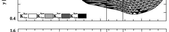
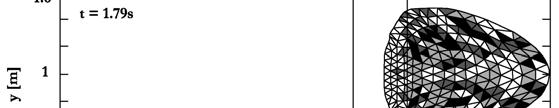
108 5.30 Figure The value of the cross-slope earth pressure coefficient (Gray et al., 1999).

109 Chapter 5: From SHWCIN to RASH 3D. Numerical model upgrade 5.31 The highest velocities are attained at the front of the avalanche and this predominantly divergent motion gives rise to active downslope earth pressures at t = 0.51 s while in the cross slope the transition from expansion to compression originates some active and passive cells. After 1 s has elapsed the avalanche spans all three sections of the chute and all the earth pressure states in the downslope and cross slope directions are activated. The front of the avalanche lies on the horizontal plane and diverges in the downslope direction, as does the granular material on the inclined section of the chute. In the run out zone, the lateral confinement ceases, the avalanche is free to expand laterally and the earth pressure coefficients change accordingly. At 1.51 s the front of the avalanche has virtually come to rest and the whole avalanche is in down slope convergence. In addition, since lateral confinement ceases on the run out plane there is strong cross slope divergence throughout most of the avalanche, with only the tip of the tail being compressed (Gray et al., 1999). The model here applied with variation of the earth pressure coefficients considers two values for K. The approach can be considered at least qualitatively correct, limits are probably due to the hypothesis that where x u + yv < 0 the flow is considered converging and the passive state applies both in x and y directions, if x u + yv > 0 the active state applies. As presented in Figure 5.25 this approach can originates only two types of mass behaviours: divergence in both directions or convergence in both directions. Figure Simultaneous longitudinal and lateral elongation (a) and longitudinal and lateral contraction (b). At the contrary, if 4 values of K had considered (see equation ) it would have been possible to have also divergence in a direction and convergence in the other one (Figure 5.26).

110 5.32 Figure Simultaneous longitudinal elongation and lateral contraction (a) and longitudinal contraction and lateral elongation (b). The obtained results are considered encouraging and qualitatively corrects. Differences as to experimental results can be explained, for example in case of δ = 30 and φ = 40, as follows. At t = 0.51 s the mass accelerates in down slope direction and the following conditions can be assumed: u v u > ; > 0 (5.20) x y x Considering the hypothesis 2a (Table 5.2, anisotropy with 2 values of K) x u + yv > 0 is obtained and K act = 0.82 is applied in down slope and cross slope directions. If the hypothesis 2b (Table 5.2, anisotropy with 4 values of K) is considered the K value in down slope direction is the same than in case 2a, and approximately the same used in case of isotropy, but in cross slope direction it is possible to have K=K a = 0.32 or K=K pass = This can modify the width of the mass along the chute. At t = 1.00 s three phases can be considered: Chute u x > v y u ; > 0 x v y < 0 ; x u + yv > 0 (5.21) Transition zone u x > v y u ; < 0 x v y > 0 ; x u + yv < 0 (5.22) u Horizontal plane > 0 x u y > 0 ; x u + yv > 0 (5.23)

111 Chapter 5: From SHWCIN to RASH 3D. Numerical model upgrade 5.33 Along the chute, as at t = 0.51 s, in cross slope direction there are both active and passive cells but elements passive in y and active in x are in prevalence. To consider only one K value in both x and y directions doesn t allow to underline distinction between convergence and divergence. On the horizontal plane the hypothesis 2a gives a K=0.82 while in the hypothesis 2b K=0.82 defines the propagation only in the down slope direction while in the cross slope K=0.32 is assumed and in fact the width is correctly reduced. At t = 1.51 s the mass decelerates in down slope direction and the following conditions can be assumed: u v u > ; < 0 (5.24) x y x Considering the hypothesis 2a x u + yv < 0 is obtained and K pass = 4.00 is applied in down slope and cross slope directions. If the hypothesis 2b is considered the K value in down slope direction is the same than in case 2a but in cross slope direction it is K=K act = 0.79 and the width becomes correctly reduced. The condition t = 1.79 s is complex, there are active and passive cells but the general behaviour determine a prevalence of active values in cross slope direction that reduces spreading of the mass. The graphic comparison between isotropy and anisotropy results helps to underline that it is useful to split the K value in x and y directions. In fact, values as K 4 allow reproducing the position of the front but in the cross slope direction becomes fundamental to use K Rheology Theoretical analysis Rheology aim is to characterize the mechanical behaviour of a material during its movement. This characterisation is usually obtained through a mathematical relation between stresses and strains of the considered material. A rheological law is made out. Several mathematical models describing the mechanics of motion of landslides have been presented in the literature (see Table 4.1). Rheological constitutive relationships applied to mass movement modelling in the past have usually been one of either Newtonian flow (e.g. Curry, 1966), Bingham flow (e.g. Sousa and Voight, 1991) or dilatant grain-flow (e.g. Takahashi, 1991). Perhaps the most well-developed group of models dealing with the flow of earth materials is based on the Bingham rheology. Jeyapalan (1981) concentrated on the special case of unsteady flow from a sudden breach of a dam and derived solutions in terms of linearly viscous (Newtonian) laminar flow and visco-plastic (Bingham) flow.

112 5.34 Dent (1982) modified an existing Newtonian unsteady flow program to accept a bilinear rheology similar to the Bingham model. The frictional rheology, where the resisting basal stress depends only on the normal stress has long been favoured in lumped mass models (see section 3.4.1). In the three dimensional frictional model developed by Sassa (1988) a two-parameter friction model for landslides, which includes the apparent sliding friction and a porepressure ratio within the moving mass, was proposed. A three dimensional model using a quadratic rheological formula containing plastic, viscous and turbulent terms was proposed by O Brien et al. (1993). A two-parameter model was developed for snow avalanche modelling by Voellmy (1955) combining Coulomb frictional and Chèzy formulas. The turbulence term, ξ, which is similar although not exactly equivalent, to the Manning n, was intended to cover all velocity-dependent factors in snow avalanche motion, including turbulence of the air-snow dispersion and air drag on the top surface of the avalanche. Koerner (1976) showed that the model offers a good simulation of velocities for rock avalanches. The applicability of the Voellmy rheology (Voellmy, 1955) has been tested by Rickenmann and Koch (1997), who found that models using a Newtonian turbulent or Voellmy fluid yielded the best simulations of channelised flows. Good empirical results obtained by Koerner (1976), Rickenmann and Koch (1997) and Hungr and Evans (1996) justify the use of the simple Voellmy model at least in the interim, until further experiments and back analyses are completed. In particular, the model developed by Hungr (1995) allows the selection of a variety of material rheologies, which can vary along the slide path or within the slide mass (see section 4.6). Some of the most recent solution methods involve the application of a more complex combination of rheologies. Iverson (1997a) describes the physics of debris flows based on the equations of motion for the flow of dry granular masses. The model is essentially a frictional one, which includes longitudinally varying internal and boundary forces as well as pore pressure Original vs. modified version of the Code Hungr and Evans (1996) applied a general dynamic model to back-analyse 23 case histories of rock avalanches. Three rheologies were tried: Frictional, Voellmy (frictional/turbulent) and Bingham. Results to date indicate that most avalanches on open slopes can be simulated satisfactorily using a friction model with pore pressure conditions that are intermediate between fully drained and liquefied. Channelised flows involving the dilution of debris by water and/or entrainment of liquefied saturated material appear to conform best to a friction-turbulent (Voellmy) mode.

113 Chapter 5: From SHWCIN to RASH 3D. Numerical model upgrade 5.35 The first criterion used to evaluate the influence of rheology was to compare the calculated and the actual length of the deposit. The friction model tends to predict deposits having the bulk of the debris proximally with excessive thinning in the distal part (Figure 5.27a). The Voellmy model generally results in uniformly distributed deposits, and moderately long deposit area with accumulation on the flatter parts of the slope (Figure 5.27b), while the Bingham model consistently overestimates the debris length. Figure A comparison of the cross-sectional distribution using (a) the friction rheology, and (b) the Voellmy rheology. A second criterion for comparing results of modelling with actual observations is in terms of velocity and flow duration. In this case the Voellmy model gives excellent correspondence between the calculated and observed velocities. Both the Frictional and Bingham models overestimate the velocities (Figure 5.28). A comparison in terms of flow duration produced a similar result. Figure Flow velocity predictions (from Hungr and Evans, 1996).

114 5.36 Of the three rheologies considered the Voellmy model produced the most consistent results in terms of debris spreading and distribution as well as velocity data. This analysis justifies the integration within the applied Code of a Voellmy rheology. It is primary to underline that the turbulent term in the Voellmy rheology assumes an importance when the velocity of the mass is high, on the contrary this term vanishes and the rheological behaviour becomes as in Frictional case. As described in section 4.5, in the applied Code dissipation is described by a Coulomb-type friction law relating the norm of the tangent traction T at the bed to the norm of the normal traction T at the bed, through a factor µ = n = Tz = σ zz b tanδ involving the dynamic friction angle δ. Having the necessity of introducing a Voellmy rheology, it is the termσ c = µ Tn that has to be modified. The original equation of σ c ( = µρgγ z h, see section 4.5.1) becomes the following: 2 v i σ c = µρg γ z h + ρg where (i = x,y) (5.25) ξ Due to the fact that with low velocity the turbulent term vanishes, the effect of a Voellmy rheology is not evident if a laboratory test is considered while in case of analysis of a real case results change. 5.6 Pore water pressure Even though lumped mass modelling is no longer useful. It is instructive to use this model to introduce the concept of energy line, as proposed by Koerner (1976). As described by Hungr, the energy line is a line raised above the movement path by an elevation equal to the kinetic energy head H k =v 2 /2g, where v is the velocity. For a block sliding on a dry frictional surface, where the resisting force is proportional to the normal force, the energy line is a straight line, inclined at the friction angle, δ (Figure 5.29). t

115 Chapter 5: From SHWCIN to RASH 3D. Numerical model upgrade 5.37 Figure Energy line (Hungr and Evans, 1996). Should pore pressure be present, the energy line will remain straight, provided that it is assumed the pore pressure, u, to be proportional to the normal stress, σ n : u=r u σ n (5.26) where r u is a proportionality constant, similar to the pore pressure ratio used in soil mechanic. The magnitude of r u is about 0.5 for full saturation and more if excess pore pressure exists. The slope of the energy line will equal to the angle, δ b : δ b = arctan[ ( 1 ru ) tanδ ] (5.27) In case of non-frictional rheology, where either the friction angle or the pore pressure ratio is not constant along the path, the energy line will be curved. If δ increases or r u decreases as a function of velocity, a concave line will result (dotted line). Koerner (1976) showed that the frictional model over-estimates the velocity in most cases of rock avalanches and snow avalanches. He adopted Voellmy s (1955) frictional/turbulent rheology, where the resisting forces are assumed to depend on the effective normal stress and the square of velocity. Presented in the same form as equation (5.27), the Voellmy relationship can be written as: 2 v δ b = arctan[ ( 1 r u ) tanδ ] + (5.28) H ξ cosψ i A concave shape of the energy line can also be obtained by allowing δ b to decrease with displacement (e.g. Sassa, 1988). A long dashed line in Figure 5.29 shows the opposite effect where the energy line is convex, predicting higher velocities for a given displacement. Such an effect could result from decrease in δ b with increasing velocity. Production of steam by means of frictional heating, or controversial mechanical fluidization phenomenon would both generate a convex energy line. Alternatively, a convex shape could result from resisting

116 5.38 forces increasing with displacement (or time), as would be the case if gradual consolidation and dissipation of pore pressure were coupled with movement (e.g. Hutchinson 1986, DeMatos 1987, Iverson and Denlinger 2001, Denlinger and Iverson 2001). All such approaches are likely to lead to an unrealistic overestimation of avalanche velocities Original vs. modified version of the Code The presence of water in the running mass is taken into account by introducing a distribution of water pressures (u) at the base of the moving mass. The values of the pressures are an input data and are given through the ratio, r u, of pore pressure to the total normal stresses at the base of the mass. The authors are aware that this is a preliminary and rough approach to the modelling of water effect on the runout. Even though this approach needs to be improved, it is considered acceptable by many authors (i.e. Hungr, 1995) for the analysis of real cases of rock avalanches. To run analyses taking into account pore pressure effects it is necessary to substitute δ b to δ in the resisting force equation of the considered rheology. If the equation T = A γ H cosψ tanδ is considered, the new equation will be i i i i i Ti = Aiγ i H i cosψ i tanδ b with δ b defined as in equation 5.27 in case of a frictional rheology and in 5.28 in case of a Voellmy rheology. As described in section 5.5.2, in the applied Code it is the termσ c = µ Tn that is modified. 5.7 Validation of the final version of RASH 3D The final version of the obtained code has been validated through numerical analysis of laboratory tests and back analysis of case histories obtained from literature. A deflected run out experiment, carried out at the University of British Columbia, has allowed verify the precision of the code in simulating the behaviour assumed by the mass on bend and in case of run up. Cases quoted in the following show as the code has also simulated in a correct way the propagation and the arrest phase of a real mass. Frank Slide and Six des Eaux Froides are two phenomena whose propagation has been characterized by a very different behaviour. In particular, in Six des Eaux Froides case the run up on the opposite slope and the wide spread of the mass induce to consider it as an interesting and complex case to be numerically analysed Deflected run out experiment A laboratory experiment was conducted at the University of British Columbia with dry polystyrene beads by McDougall and Hungr (2004). The material was released

117 Chapter 5: From SHWCIN to RASH 3D. Numerical model upgrade 5.39 from a box onto a chute with variable slope (to control the approach velocity), ran out onto a 20 approach slope and was deflected by a dike oriented obliquely to the flow direction. The deflection angle, λ (plan angle between the initial direction of motion and the intersection of the dyke and approach planes), and the dike dip angle, ψ d, were variable. A photograph of the laboratory apparatus is shown in Figure The box used to contain and release the material at start up could not be replicated by a digital 3-D sliding surface, due to its infinitely sloping sidewalls. Therefore, an imaginary release chute and initial distribution of material were used by McDougall. By trial and error, the position, width and velocity of the simulated flow front were synchronized with the experiment at the start of the 20 approach slope. Figure Photograph of laboratory apparatus used for deflected runout experiments (Image courtesy of S. McDougall, University of British Columbia). A simulation of an experiment configured with λ = 60 and ψ d = 33 is shown in Figure 5.31, were laboratory results and McDougall numerical analyses are compared to the results obtained using RASH 3D. As in McDougall s analyses a frictional rheology with δ =20 and φ=25 has been applied. These friction angles are within a small range of values measured in separate laboratory tests by McDougall, placing a conical pile of beads on a sheet metal plane and, respectively: 1) measuring the tilt angle that initiates basal sliding, and 2) measuring the angle of repose of the material itself. With rheological parameters calibrated on the basis of the previous test (δ =20 and φ=25 ) the model RASH 3D produces accurate predictions of maximum runup distance, as well as the position and distribution of slide material at that instant. A comparison of observed and predicted maximum runup distances is shown in Figure 5.31.

118 5.40 t= 0.0 s A B t= 0.2 s t= 0.4 s t= 0.6 s Figure Analysis of a deflected runout experiment using λ=60 and α d =33. Column A, RASH 3D results. Column B, McDougall results. The planes are marked with a 10cm square grid (Photographs courtesy of S. McDougall, University of British Columbia).

119 Chapter 5: From SHWCIN to RASH 3D. Numerical model upgrade Frank slide (Canada) On April 29, 1903 approximately 30 million m 3 of rock descended Turtle Mountain into the Crowsnest River valley, partially burying the town of Frank, Alberta and killing 70 people. It was Canada s worst landslide disaster. Figure 5.32 Frank Slide event. The original sliding surface and the starting position of the 30 million m 3 slide mass have been approximated using detailed digital elevation data provided by the Geological Survey of Canada as well as historical photographs and maps (Figure 5.33). t =0 s Figure 5.33 Frank Slide digital elevation model. The model has been applied using a frictional rheology with a basal friction angle δ = 14 and an internal friction angle φ =40.

120 5.42 t = 20 s t = 40 s t = 60 s t = 80 s Figure 5.34 Numerical analysis with RASH 3D. Dash line represents the boundaries of the real runout area.

121 Chapter 5: From SHWCIN to RASH 3D. Numerical model upgrade Six des Eaux Froides (Switzerland) In 1946 approximately 6 million m 3 of rock descended the Andin valley (near Rawyl, Valais, Switzerland), burying the Luchet Lake located in the bottom of the valley (Figure 5.36). Figure 5.35 Six des Eaux Froides landslide (Image courtesy of CREALP, Sion Switzerland). The original sliding surface and the starting position of the mass have been approximated using detailed digital elevation data provided by the CREALP (Switzerland) as well as historical photographs and maps. Figure 5.36 Luchet Lake before and after the landslide (Images courtesy of CREALP, Sion Switzerland). The model has been applied using a frictional rheology with a basal friction angle δ = 17 and an internal friction angle φ =40 (Figure 5.37).

122 5.44 t=0s t=10s Figure 5.37 Numerical analysis with RASH 3D. Dash line represents the boundaries of the real runout area

123 Chapter 5: From SHWCIN to RASH 3D. Numerical model upgrade 5.45 t=20s t=30s Figure 5.37 (Cont.)

124 5.46 t=40s t=50s Figure 5.37 (Cont.)

125 Chapter 5: From SHWCIN to RASH 3D. Numerical model upgrade 5.47 t=60s t=70s Figure 5.37 (Cont.)

126

127 Chapter 6 DAN. Back analyses of case histories 6.1 Introduction Whatever the applied analytical model, results of a numerical simulation depend on the value assigned to each constitutive parameter of the assumed rheology before running the analysis. To define a range of typical values for these parameters, the numerical code DAN (Hungr, 1995) has been applied to back analyse a set of case histories of rock avalanches selected from literature. Before creating the geometrical model, to be used to run numerical analyses, each case has been carefully analysed and all the available information have been collected in a filing table. Some data are fundamental to characterize the general behaviour of each considered case and have to be taken into account when values obtained from back analyses are used to simulate a potential landslide, only cases having similar characteristics (e.g. run out area shape, material type, glacier along the path) can be compared. Some other data are important to calibrate the model. For this purpose information concerning the position of the proximal and distal points and the depth of the mass in the deposit, the mean or maximum velocity reached along the path, the presence of run up on bend or on an opposite slope and so on are fundamentals. A back analysis procedure gives the possibility of calibrating the model in order to obtain the best value that has to be assigned to each of the required rheological parameters.

128 6.2 As previously mentioned, the obtained results could be useful in run out prediction of a potential landslide. To proceed in this direction, it is beforehand necessary to verify that DAN results can be used as input data in a different numerical code, like RASH 3D. Cases for which a DEM pre-collapse was available have been analysed with both DAN and RASH 3D. Results have been encouraging and have justified the use of a coupled methodology in which DAN is applied to run back analyses while RASH 3D is useful for prediction of propagation on a complex topography. 6.2 Collection and cataloguing of case histories Numerical simulations should provide a useful tool for investigating case histories if some geometrical data and some characteristic information of the analysed case are known. Cases selected from literature are well documented for the purposes of the present work if available geometrical data consist at least of a simple topography, containing information about the shape of the run out area and the boundary of the unstable area, and a profile along the path of the movement, from which it emerges the position of the deposit and of the initial volume (Figure 6.1). Figure 6.1. Val Pola rock slide (Erismann and Abele, 2001). An advantage in using DAN is due to the fact that, among the required input data to run a back analysis, a DEM (Digital Elevation Model) is unnecessary. In fact, the above listed information is exhaustive enough to generate the geometrical model. This

129 Chapter 6: DAN. Back analyses of case histories 6.3 allows the back analysis of many of the cases obtained from literature, whose analysis would be impossible with a code in which a digital elevation model is required. For each case, collected data can be subdivided in two main groups: - Classification parameters, containing information known before the event (e.g. material type, average slope angle, bedrock of the area, vegetation); - Control parameters, containing information known only after the event (e.g.. run up, velocity, final front and rear positions, run out area shape). To organize all the available information in an organic way and to guarantee that the main aspects of each case could immediately emerge, a filing table has been prepared (Figure 6.2). This table contains different sections, some of which collect data necessary to compare the characteristics of a back analysed case to those of a potential landslide (only cases having similar characteristics can be compared): - General aspects, in which information on type (e.g. rock avalanche, debris flow... ) and the geographical location of the event is quoted together with details concerning causes and consequences of the propagation (if known). In particular, sites not far one from the other or having similar triggering mechanism could have a similar behaviour. - Geometry, containing data from which it eventually emerges a different behaviour of the mass along different portions of the path and it is possible to determine the run out area shape and to obtain the geometrical model to be used as input in DAN (e.g. profile and topography before and after the event). It could be interesting and useful to compare cases having a similar propagation and a similar run out area shape (see section 6.2.1). - Morphology, in which are summarized all the information concerning the type of material existing along the path and within the mass, together with indication of any further entrainment of material during propagation. Comparing cases it could be important to know if the involved material is, for example, pyroclastic or gneissic. These could be one of the aspects that modify the behaviour of the mass. It is also important to underline if there is a glacier along the path and if water is clearly involved or not. Some others collect information necessary to compare the reconstructed geometry and the back analysis results to the real configuration of the slope and to the shape assumed by the deposit: - Geometrical details, aspects concerning the volume involved, the average slope angle along the path or in correspondence of the failure sector (obtained connecting the uppermost point from which the rock mass broke away and the toe of the surface

130 6.4 of rupture). Useful can also be information concerning the orientation of the sliding surface. - Run out details, data characterising the propagation phase. To calibrate the model during back analysis it is fundamental to know the final position reached by the mass (proximal and distal point of the deposit), further information concerning the velocity reached along the path and the existence of run up in bend or on the opposite slope can help to determine the real behaviour during propagation in a more detailed way. Finally, the last section (Bibliography) is devoted to list the source of the information concerning the described case. Figure 6.2. Example of filing table containing information about each analysed case.

131 Chapter 6: DAN. Back analyses of case histories General characteristics Cases having different characteristics are probably characterized by a different behaviour during the run out phase. It is important to focus on those aspects that seem to influence more than others the propagation phase of the unstable mass. When a potential event has to be simulated, this distinction can help in the choice of those back analysed cases that can be compared to the analysed event and should reduce the range of values to be assigned to the rheological parameters. The aim of this type of approach is to obtain the results as more realistic as possible. The main aspects on which attention has been focused on are the following: - Landslide volume (V). In a landslide phenomenon mobility seems to increase with volume. Compared to a rock fall event (V<10000 m 3 ), the motion of rock avalanches is more massive and the bulk of rock fragments moves as a semicoherent flowing mass. - Run out area shape (Figure 6.3). It introduces three different sub-classes as a function of the shape assumed by the run out area. The considered categories are the following (Nicoletti and Sorriso-Valvo, 1991): - Elongated shape (A). This generally occurs when there is a narrow valley down which the debris is channelized. - Tongue shape (B). This occurs when the moving debris is free from lateral constraints and is able to stop spontaneously when it comes to a wide valley or plan. - T shape (C). This shape results from the crossing of a narrow valley followed by a perpendicular impact against the opposite slope. Run up and partition of the debris are common features. Figure 6.3. Run out area shape.

132 6.6 - Material type. For the intact rock pieces, the generalised Hoek-Brown failure criterion for rock jointed masses (Hoek & Brown, 1980) is simplified to: 0.5 ' ' ' σ3 1 = σ3 + σci mi + 1 σ ci σ (6.1) where σ 1 and σ 3 are the maximum and minimum effective stresses at failure respectively, m i is the value of the Hoek-Brown constant m for the intact rock, 1 and 0.5 are the characteristic constants of the rock mass in case of intact rock, and σ ci is the uniaxial compressive strength of the intact rock pieces. In order to use the above mentioned criterion for estimating the strength and deformability of jointed rock mass, σ ci and m i have to be estimated (Hoek & Brown, 1997). When laboratory tests are not possible, Table 6.1 can be used to obtain estimate of σ ci and m i of the intact rock pieces in the rock mass. On the base of this criterion, the material type classification can subdivide the cases as a function of UCS as indicated in Table 6.1. Table 6.1. Field estimates of uniaxial compressive strength (Hoek and Brown, 1997).

133 Chapter 6: DAN. Back analyses of case histories 6.7 The behaviour of a rock mass probably changes as a function of the type of material involved, fragmentation and desegregation could be more rapid in a weak material than in a strong one. - Slope characteristics. The path followed by a mass during propagation can be characterized by presence of vegetation (e.g. forest), debris or intact rock. Probably events with a reduced volume are more influenced from differences in slope characteristics respect phenomena involving a large volume. The existence of water (e.g. superficial or due to infiltration) can determine saturation of the material and deeply modify the final configuration of the deposit. Ice (e.g. glacier) along all or part of the travel path reduces or vanishes the basal resistance term increasing velocity of propagation and changing the final distribution assumed by the debris. It is then important to distinguish cases in which ice or water have played an important role from those cases in which propagation was in dry conditions. 6.3 Back analysis procedure The back analysis procedure can be subdivided into 6 steps (Figure 6.5): 1. Digital reconstruction of the topography. The slope profile geometry, the profile of the top of the initial mass and the path width are described by a series of x (distance), y (elevation) and z (width) points, respectively (Figure 6.4). 2. Choice of the values to be assigned to the characteristic parameters of the assumed rheology. 3. Run of the analysis. 4. Comparison between the results obtained through the simulation (B in Fig 6.5) and the actual characteristics of the deposit (A in Fig.6.5). 5. If B is too different from A: Change of the value assigned to the rheological parameters 6. Report of the obtained results.

134 Elevation [m] Width [m] Distance [m] Figure 6.4. Digital reconstruction of the topography using DAN. The material rheology has been assumed as frictional (see section 4.4 and 5.5). Friction angle (δ) and pore water pressure (r u ) are the only rheological parameters that have to be calibrated. The remaining variables, held constant in all the analyses. In a first hypothesis a dry condition (r u =0) is assumed and only the value of δ is varied to better simulate the real behaviour of the mass. A second hypothesis considers the mass as saturated (r u =0.5). Finally, if there are some portions of the path covered by a glacier r u =0 and two values of friction angle: δ 1 where there is no ice, δ 2 =0.6 where there is ice. In this case, δ 1 corresponds to δ b are assumed. The aim of this double analysis is to guarantee that water content is not neglected. A friction angle value too low is probably an index that no water assumption is unrealistic for the examined case. The main results of each analysis were systematically recorded. Each trial run was assessed by matching the following parameters to the actual values as determined from maps or from the reports of the case histories: total horizontal run out distance, length of the main deposit, mean thickness of debris, flow velocities and flow duration (where available).

135 Chapter 6: DAN. Back analyses of case histories 6.9 The above parameters could not always be obtained from the case history record, by consequence the comparisons were carried out opportunistically wherever data was available (Hungr and Evans, 1996). Figure 6.5. Back analysis procedure. The best match parameters were sought to produce mainly the correct run out, while at the same time obtaining the best possible match in term of velocities and duration (e.g. Table 6.2). Madison Canyon Data Literature Analysis Volume 10 6 [m 3 ] Rear final position [m] Front final position [m] Fahrböschung [ ] Velocity [m/s] Table 6.2. Madison Canyon rock avalanche. Example of analysis results.

136 Validation of the coupled methodology Trying to reduce the uncertainty range of values to be assigned to rheological parameters, a methodology in which DAN is used to run back analyses of case histories and RASH 3D is applied to predict propagation of a mass on a complex topography is proposed. To consider rheological values obtained with DAN as guidelines in assigning values to rheological parameters in RASH 3D it is beforehand necessary to verify that DAN results can be used as input data in a different numerical code, like RASH 3D. Cases for which a DEM pre-collapse was available have been analysed with both DAN and RASH 3D. Results have been encouraging and have justified the use of the proposed coupled methodology. Frank Slide (Canada) and Six des Eaux Froides (Switzerland) are two examples having run out with a very different configuration. Analyses shown in Section 5.7 have been carried out assuming a frictional rheology in which values assigned to rheological parameters are those previously obtained with DAN. Both cases are simulated in a satisfactory way. 6.5 Results of back analyses After validation of the proposed methodology (see section 6.4), DAN has been widely applied to the back analysis of as many case histories as possible. The back analysis procedure has been more accurate when detailed data, characterising the propagation phase, were supplied (e.g. proximal and distal points and the depth of the mass in the deposit, mean and/or maximum velocity reached along the path, presence of run up on bend or on an opposite slope). Some of this information has been fundamental to guarantee a more accurate analysis and more reliable results. In Table 6.3 are summarized the best match parameters for the analysed cases, some of which were also analysed by Hungr in the past (Hungr & Evans, 1996). As described in section 6.3 each case has been analysed assuming r u = 0 and r u = 0.5, respectively and introducing a second value of friction angle where the path was covered by ice (e.g. Felik and Pandemonium Creek). Even though both Felik and Pandemonium Creek have a portion of the path covered by glacier, for each case the variation of δ 1 value respect the obtained δ b value is deeply different. To think that these two cases are similar and by consequence to compare their behaviour it would be wrong. Analysing available information it emerges that in Felik case the mass run on ice in about the entire path, in Pandemonium Creek case, at the contrary, only a short portion of the whole path is covered by ice. This is an example of the attention that has to be put in the analysis of each considered case.

137 Chapter 6: DAN. Back analyses of case histories 6.11 Frictional rheology Country Site Material type r u = 0 r u = 0.5 Glacier (r u = 0) δ [ ] δ [ ] δ 1 [ ] δ 2 [ ] Conturrana Sedimentary Scanno Sedimentary ITALY Vajont Sec E-E Sedimentary Vajont SecF-F Sedimentary Val Pola Metamorphic Felik Metamorphic Charmonetier Metamorphic 39 FRANCE La Madeleine Metamorphic Claps de Luc Sedimentary Flims(pleistocene) Sedimentary 9 20 SWITZERLAND Flims(1939) Sedimentary Six Eaux Froides Elm Metamorphic Avalanche Creek Volcanic Dusty Creek Volcanic Avalanche Lake N. Sedimentary 7 (1) 14 Avalanche Lake S. Sedimentary 8 (1) 15 CANADA Eagle Pass Metamorphic 30/38 ( Nomash River Sedimentary Pandemonium Creek Metamorphic Rubble Creek Volcanic JAPAN Mt. Ontake Volcanic 8 17 Table 6.3. Results of the back analyses. (1) back analyses are carried out assuming the Hungr s hypothesis of absence of glacier filing the bottom of the valley this requires a run up of about 650m on the opposite slope justifying a so low friction angle (see Annex - Avalanche Creek), (2) there are two hypotheses on Eagle Pass run out (see Annex Eagle Pass) in the first hypothesis the mass reaches the bottom of the valley in one phase (30 ), in the second one two phases characterise the movement, the mass initially stops along the slope (38 ). Mt. Ontake (Japan) represents a very particular case, a mass changing from 15 million m 3 to 30 million m 3 ran for about 12 km along a river and the involved material is totally saturated. Since some cases originated long time ago (e.g. Conturrana, Flims(Pleistocene), La Madeleine, Scanno) a certain degree of uncertainty on the available information is probable. When results obtained through back analyses of these cases are used as guidelines this aspect does not have to be neglected. 2)

138 6.12 Cases as Avalanche Lake and Eagle Pass have contrasting interpretations. In the present work, back analysis of these cases has been realized following Hungr s hypothesis (see Appendix A). Main difficulties, on which it has been run into carrying out the analyses, have induced to deeply reflect on the influence that the presence of water can determine on the obtainable results. Indeed water assumes a particular effect not only in the triggering phase but also along the path of propagation. The presence of a river, crossed by the mass or along which the mass is channelized, can deeply modify the shape of the deposit, the distance of propagation and the reached velocity. Similar behaviour can be obtained with the entrainment of a large quantity of saturated material. If the three classes, introduced by Nicoletti and Sorriso-Valvo in 1991, about the runout area shape are considered (see Figure 6.3), it emerges that the rheological values obtained with the frictional rheology increase changing from elongated to tongue shapes, passing through T shape. Detailed results are quoted in Table , respectively. Frictional rheology Site Date r u = 0 r u = 0.5 δ [ ] δ [ ] Nomash River Pandemonium Creek (3) Rubble Creek Table 6.4. Results of the back analyses on cases having elongated shape run out area. (3) the case of Pandemonium Creek has a portion of the path covered by glacier but the limited extension could justify that it is compared to results in which ice is absent. Frictional rheology Site Date r u = 0 r u = 0.5 δ [ ] δ [ ] Claps de Luc Charmonetier Flims(1939) Eagle Pass /38 Conturrana 4th century 16 (4) 30 Table 6.5. Results of the back analyses on cases having tongue shape run out area. (4) the case of Conturrana originated in the 4 th century, results could be affected by a certain degree of uncertainty.

139 Chapter 6: DAN. Back analyses of case histories 6.13 Frictional rheology Site Date r u = 0 r u = 0.5 δ [ ] δ [ ] La Madeleine post glacial Vajont Sez. E-E Vajont Sez. F-F Val Pola Scanno 217 B.C.? (5) Elm Table 6.6. Results of the back analyses on cases having T shape run out area. (5) the case of Scanno originated probably in 217 B.C., results could be affected by a certain degree of uncertainty. In Table 6.7 it further emerges as all the considered parameters assume a mean value that increases changing from Elongated shape to Tongue shape. δ [ ] Elongated T shape Tongue min mean max Table 6.7. Distribution of resistance parameters as a function of the run out area shape. In this sense the classification introduced by Nicoletti seems to be respected in the carried out analyses. However, it has to be taken into account that the shape assumed by the deposit is influenced both by the topography and by the characteristic of the moving mass (e.g. presence of water). An elongated deposit (A) probably derives by a saturated material, mass is channelized along a narrow valley where a river is probably present. At the contrary, a tongue deposit (B) could be obtained with a dry material, the mass could not be able to reach the bottom of the valley and in this case less water or saturated material is probably involved in the movement. Finally, a T shape deposit (C) can be considered in some way intermediate between (A) and (B). A portion of the whole path can be considered as in situation (A) while the other more similar to situation (B). This could justify intermediate values of friction angle. Any way it has to be underlined that empirical methods, as those considered by Nicoletti, are unable to take into account the water effect. The code DAN used to run back analyses in the present work is able to consider the real width of the channel of propagation of the mass and can incorporate in the bulk friction angle the water effect.

140 6.14 Trying to subtract the water effect from the friction angle, a pore pressure different from zero can be introduced. But it is difficult to define which had really been the influence assumed by the water in each case. What can be suggested could be to use lower values of r u in case of tongue shape and higher values in case of elongated shape. More work is needed to better characterize the influence of water in the back analysed cases. In fact, once subtracted the water effect by the friction angle: 1) the runout area shape effect could be reduced; 2) a certain influence of material type could emerge. Furthermore, before trying to obtain possible correlations among friction angle, volume, shape, material type and slope characteristics the back analysis of a higher number of cases is required in future. 6.6 Observations The DAN code allows to simulate the main features of all the considered case histories. To reduce a complex and heterogeneous three dimensional problem into an extremely simple formulation allows to run simulation on many case histories obtained from literature, cases for which a DEM is not available. The path width is an input data but working on back analyses and not on prediction this data is always known if a simple topography is given. The simplicity of the model is an advantage in making possible an immediate and rapid numerical simulation of real cases. To obtain useful guidelines to the choice of values to assign to resistance parameters of a potential landslide it is important to increase the number of back analysed cases.

141 Chapter 7 Conclusions and further developments p Flow-like landslides are among the most destructive and difficult to prevent types of landslide phenomena. Their impact is becoming stronger and stronger due to increasing tourism and the construction of new roads and railways in mountainous areas (Bonnard et al., 2004). With prediction losses could be reduced, as they could provide means to define the hazardous areas, estimate the intensity of the hazard and work out the parameters for the identification of appropriate protective measures. At the same time, reliable predictions of run out could help to avoid exceedingly conservative decisions regarding the development of hazardous areas. Dealing with the run out problem, it has been observed that a continuum mechanics approach is flexible enough to allow that many of the aspects characterising propagation of a mass on a complex topography can be taken into account. Any way, a numerical code is never finished. It develops and when a problem is solved a new one originates. The SHWCIN code, which is at the base of the present work, has been thoroughly modified and now the new version, RASH 3D, is able to answer in a correct way different analysed conditions. First three dimensional analyses carried out with SHWCIN gave asymmetric results also when symmetric conditions were imposed. A change of the type of adopted mesh solved this problem without increasing of CPU-time. Afterward the analysis of a real topography was introduced. To take into account its effect on the behaviour of a mass during propagation, it was necessary to introduce variation of the gravity vector components as a function of the slope local trend has.

142 7.2 Satisfactory results have been obtained, the behaviour assumed by the mass on complex surfaces looks correct both in case of laboratory tests and of real sites analyses. To further validate the gravity effect, analyses of run up have been carried out, results are again corrects both in case of run up on bend and on opposite slope with respect to the slope from which mass detached. It could seem strange but major problems have been observed not analysing a complex topography but considering a simple inclined or horizontal plane. In this condition the mass is not obliged to follow a certain path, not being influenced by a particular trend of the slope it will mainly assume its natural behaviour and degree of spread. To reduce mistakes in obtained results it has been fundamental to understand the real influence of earth pressure coefficients and introduce anisotropy of normal stresses. Simulations carried out on laboratory tests have been valuable to underline the necessity of separating the behaviour of the mass along the direction of propagation with respect the direction transversal to it. To approximate the real behaviour of a mass, a constitutive law has to be assumed. Each law is characterised by a certain number of parameters. Value to be assigned to each parameter has to be defined before running the analysis. Difficulties in choosing these values are due to the absence of a mass with a standard behaviour. To consider simple rheologies, characterized by a little number of parameters, becomes fundamental. The original version of the code used a frictional rheology in which the only required parameter is the basal friction angle. To better simulate the propagation phase the possibility of taking into account the eventual pore water effects has been introduced. To compare the obtained results to those obtainable with a different rheology, a Voellmy rheology has been numerically implemented. It emerges that deposited mass changes its distribution and maximum velocity is lower than that touched assuming a frictional rheology. Before going on with a new step, each change has been carefully tested and validated through numerical simulation of laboratory tests and back analysis of case histories. The carried out analyses underline as whatever the applied analytical model, more or less complex, results depend on the value that is assigned to the characteristic parameters of the assumed rheology. To define a range of typical values for these parameters, the numerical code DAN has been applied to back analyse a set of case histories of rock avalanches selected from literature. Some data characterising the general behaviour of each considered case have to be taken into account when values obtained from back analyses are used to simulate a potential landslide it is important to keep in mind that only cases having similar

143 Chapter 7: Conclusions and further developments 7.3 characteristics (e.g. run out area shape, material type, glacier along the path) can be compared. Before employing energies on the analysis of as many cases as possible and on the creation of a database collecting them, it has been necessary to verify that DAN results can be used as input data in a different numerical code, like RASH 3D. Cases for which a DEM pre-collapse was available have been analysed with both DAN (with a simplified topography) and RASH 3D (with the real topography). Results have been encouraging and have justified the use of a coupled methodology in which DAN is applied to run back analyses while RASH 3D is useful for prediction of propagation on a complex topography. Further developments of the research work undertaken are needed. These have to be done by keeping in mind the final objective, which is to provide a tool whose application could give useful information for investigating, within realistic geological contexts, the dynamics of flows and of their arrest phase. As regards the RASH 3D code the main aspects that have to be further investigated concern the entrainment of material along the path of propagation, the possibility of having at the same time a multiple detachment of mass from different places of the slope and a condition of anisotropy of normal stresses that compared with the actual formulation guarantees all the possible combinations of divergence and convergence along two normal directions (i.e. K x K y ). Concerning DAN, it is fundamental to increase the number of carried out back analyses. A wide database should guarantee a higher possibility that cases having similar characteristics are contained. Similar events can be compared each other and obtained information can be more attainable when used as guideline for the analysis of an equivalent potential landslide.

144

145 Appendix A Analysed case histories Name: AVALANCHE CREEK (MT CAYLEY) Origin: Volcanic site Classification: Rock avalanche Debris Flow Where: Mount Cayley, British Columbia, Canada When: 1984 The slope had undergone substantial deformations for at least Triggering: Yes 10 years before failure. The debris flow was associated with the largest rainstorm of the summer No The rock avalanche destroyed vegetation along the path. A part of the Consequences: mass travelled over the 1963 debris into Dusty Creek probably blocking it. The debris flow swept away a logging road bridge at the mouth of Turbid Creek and temporarily dammed the Squamish River. GEOMETRY

146 II (modified from Evans et al., 2001) 1 phase: rock avalanche 2 phase: debris flow Bedrock of the area: MORPHOLOGY Rock avalanche Avalanche Source Creek Subvolcanic, pyroclastic rock Dacite, tuff and pyroclastic breccia Colluvial material, snow, ice Turbid Creek Material entrained along the path: Mantle: Forest Forest Debris The melting snow and ice could have saturated the Water: small volume of debris. Travelled on a main track covered by metres of snow and ice. Debris flow Landslide debris Chunks of ice Volume [m3]: Slope angle [ ] GEOMETRICAL DETAILS V initial 0.88*10 6 (0.74* %) Rock avalanche V final 1.08*10 6 Debris flow Path: Source: 40 1*10 6 (most of the rock avalanche debris transformed into a distal debris flow) See figure

147 Annex A III Failure surface slope [ ] Run out area shape: Velocity [m/s] Time [s] Deposit Thickness [m]: 5 A Max: RUN OUT PHASE Debris flow Average: 10 Upper-path 70 Rock Avalanche Creek/ avalanche Turbid Creek Point R in the figure ore (debris flow) xfront [m]: See figure xrear [m]: See figure Run up [m]: On bend Fahrboschung [ ]: 19 (rock avalanche) In the opinion of Evans et al. (2001) the rock avalanche did not come to a halt in the upper part of its path as suggested by Note: Cruden and Lu (1992) but travelled to its distal limit in one uninterrupted movement. BIBLIOGRAPHY Evans, S. G., Hungr, O., Clague, J. J., Dynamics of the 1984 rock avalanche and associated distal debris flow on Mount Cayley, British Columbia, Canada; implication for landslide hazard assessment on dissected volcanoes. Engineering Geology, 61, pp Evans, S.G., Jordan, P., A hyper-mobile debris avalanche from the western flank of Mount Cayley volcano, British Columbia and associated debris flows. (Manuscript in preparation). Cruden, D. M., Lu, Z. Y., The rockslide and debris flow from Mount Cayley, B. C., in June Can. Geotech. J., 29, pp Lu Z. Y., Cruden D. M., Two debris flow modes on Mount Cayley, British Columbia. Can. Geotech. J., 33, pp

148 IV Name: Origin: Classification: Where: When: Triggering: Consequences: Glacial site Rock avalanche AVALANCHE LAKE Mackenzie Mountains, Backbone Ranges, Canada - Late Pleistocene (Kaiser and Simmons, 1990) - Holocene sometime after 1450 (Evans et al., 1994) Yes No Unknown Lakes have formed where drainage has been impedded by debris. (e.g. south lobe has dammed drainage to form South Lake) GEOMETRY (modified from Evans et al., 1994)

149 Annex A V Source MORPHOLOGY Main deposit Devonian carbonate dolomite Bedrock of the area: Lower devonian Middle carbonate devonian dolomite dolomite Material entrained along the path: Mantle: Water: Shelf lobe (reverse slope) Limestone and shale Alluvial deposits and conifer fragments Vegetation South lobe (reverse slope) Limestone and shale Vegetation absent Forested at that time absent Vegetation absent The mobility exhibited by debris on the Shelf may have been assisted by snow on the ground or by the presence of saturated ground due to thawed permfrost Volume [m3]: Slope angle [ ] Failure surface slope [ ] GEOMETRICAL DETAILS Vinitial 200*10 6 Shelf above Avalanche 5*10 Lake (Shelf lobe) 6 Vfinal Avalanche Lake valley 155*10 (Main deposit) 6 South valley (South lobe) 40*10 6 Path: Source: 30 Run out area shape: Velocity [m/s] Time [s] C RUN OUT PHASE Max: 80 Average: Deposit Thickness [m]: 50 (Main deposit) xfront [m]: Run up [m]: On the opposite valley side and in the reversing direction again xrear [m]: Fahrboschung [ ]: 8 (Shelf lobe); 10 (South lobe)

150 VI Note: In the opinion of Kaiser and Simmons (1990) a glacier ice partially filled the valley while Evans et al. (1994) think that the avalanche occurred in an ice-free environment BIBLIOGRAPHY Kaiser, P. K., Simmons, J. V., A reassessment of transport mechanisms of some rock avalanches in the Mackenzie Mountains, Yukon and Northwest Territories, Canada. Canadian Geotechnical Journal, Vol. 27, pp Evans, S. G., Hungr, O., Enegren, E. G., The Avalanche Lake rock avalanche, Mackenzie Mountains, Northwest Territories, Canada: description, dating, and dynamics. Canadian Geotechnical Journal, Vol. 31, pp

151 Annex A VII Name: Origin: Glacial site CHARMONETIER Classification: Rock avalanche Where: Taillefer Mountain, Romance Valley, Charmonetier (Lyon), France When: August 24 th, 1987 Triggering: Consequences: Yes Rain + Existence of abandoned quarry No Breakage of the road. The debris stripped away vegetation. (Couture et al., 1997) GEOMETRY MORPHOLOGY Source Path Deposit Bedrock of the area: Amphibolites Amphibolites/Granite Alluvial soil Material entrained along the path: Weathered amphibolites and trees Mantle: Forest Forest Forest

152 VIII Water: Rain in the days before probably the debris wasn t dry GEOMETRICAL DETAILS Volume [m3]: 0.13*10 6 Slope angle [ ] Failure surface slope [ ] Run out area shape: Velocity [m/s] - Time [s] - Deposit Thickness [m]: B Path: Source: RUN OUT PHASE Higher near the later boundary of the corridor, lower in the central part xfront [m]: 600 xrear [m]: 200 Run up [m]: No Fahrboschung [ ]: 41 Existence of intermittent streams and water infiltrations in the Note: detachment area BIBLIOGRAPHY Couture, R., Antoine, P., Locat, J., Hadjigeorgiou, J., Evans, S. G. and Brugnot, G., Quatre cas d avalanches rocheuses dans les Alpes francaises. Can. Geotech. J., 34, pp

153 Annex A IX Name: Origin: Classification: Where: When: 1442 Triggering: Consequences: Glacial site Rock avalanche Luc-en-Diois, Drome, France Yes CLAPS DE LUC No Blockage of the Drome river with formation of a little and a big lakes now disappeared GEOMETRY (Couture et al., 1997) MORPHOLOGY Source Path Deposit Limestone, marne Bedrock of the area: Limestones alternate with marne Material entrained along the path: Mantle: Forest Forest Forest Water: In a dry condition probably triggering would have been impossible

154 X Volume [m 3 ]: 2*10 6 Slope angle [ ] Failure surface slope [ ] Run out area shape: B GEOMETRICAL DETAILS Path: 30 Source: RUN OUT PHASE Velocity [m/s] Max: Average: Time [s] - Deposit Thickness [m]: xfront [m]: 800 xrear [m]: Run up [m]: no Fahrboschung [ ]: Note: Initial mass slided as a slab BIBLIOGRAPHY Couture, R., Antoine, P., Locat, J., Hadjigeorgiou, J., Evans, S. G. and Brugnot, G., Quatre cas d avalanches rocheuses dans les Alpes francaises. Can. Geotech. J., 34, pp Ramirez, A., Fabre, D., Antoine, P, Enseignements tires de deux ecroulements par glissement couche sur couche en terrain calcaire. Compte rendu, 5 e Symposium International sur led glissement de terrain, Lausanne. A.A. Balkema, Rotterdam. pp

155 Annex A XI Name: Origin: Classification: Where: When: Triggering: Consequences: (Nicoletti and Parise, 1996) Rockslide Debris flow CONTURRANA Capo San Vito (peninsula of NW Sicily) 4 th century Yes Earthquake and presumably groundwater pressures No GEOMETRY Bedrock of the area: Material entrained along the path: Mantle: Water: MORPHOLOGY Source/Rock slide Carbonate rock Indurated breccia of limestone fragments with a plastic complex (clayey-silty, sandy material) in the basal part There are some springs Debris flow The succession of formations involved, plastic complex surmounted by breccia is preserved in the deposit

156 XII Volume [m 3 ]: 22*10 6 Slope angle [ ] Failure surface slope [ ] Run out area shape: B Velocity [m/s] Time [s] - Deposit Thickness [m]: Path: GEOMETRICAL DETAILS Source: 20 Deposit: 11 2 (debris flow) RUN OUT PHASE Max: - Average: - - x front [m]: 1590 x rear [m]: 300 Run up [m]: No Fahrboschung [ ]: - The landslide deposit consists of 2 parts: the remnants of the Note: rockslide mass, still resting upon the rupture surface above the cliff, and the debris flow deposit, extending in front of and below the cliff. BIBLIOGRAPHY Nicoletti, P. G., Parise, M., Geomorphology and kinematics of the Conturrana Rockslide-Debris Flow. Earth surface processes and landforms, Vol. 21, pp

157 Annex A XIII Name: Origin: Classification: Where: Volcanic site Rock slide - Debris flow DUSTY CREEK (MT CAYLEY) Mount Cayley, British Columbia, Canada When: July 1963 Geological setting + Deterioration of the slope over a Yes long period of time until a triggering due to earthquake Triggering: or storm No Turbid Creek and Dusty Creek were blocked and lakes formed behind the debris. Debris dam soon overtopped Consequences: causing floods and probably debris flow. The debris stripped away vegetation. GEOMETRY (modified from Evans et al., 2001) Bedrock of the area: MORPHOLOGY Source Along Dusty Creek Along Turbid Creek Subvolcanic, Pyroclastic rock Poorly consolidated Dacite, lapilli tuff, Granodiorite, quartz tuff breccia and breccia, granodiorite, diorite, gneiss dacite, lapilli tuff gneiss Involved material: Material entrained Vegetation, granodiorite, lapilli, ash along the path: Mantle: Heavely forested Forest Forest

158 XIV Water: Little water was involved in the flow. It is unlikely that there was snow or ice on the main track. Volume [m3]: 5*10 6 Slope angle [ ] Failure surface slope [ ] Run out area shape: A Velocity [m/s] Path: GEOMETRICAL DETAILS Source: Max: Time [s] RUN OUT PHASE Average: Along Dusty Creek (Dusty Creek); 12 (Turbid Creek) Along Dusty Creek up to 70 Deposit Thickness [m]: Along Turbid up to 65 Creek xfront [m]: 2400 xrear [m]: - Run up [m]: On bend Fahrboschung [ ]: 17 It exist deposit only along Turbid Creek (about 1km long). Total path about 2500 m. Note: Quick fragmentation generates angular to subrounded clasts in a matrix of silt and sand BIBLIOGRAPHY Clague, J. J., Souther, J. G., The Dusty Creek landslide on Mount Cayley, British Columbia. Canadian J. of Earh Sciences, 19, pp Lu Z. Y., Cruden D. M., Two debris flow modes on Mount Cayley, British Columbia. Can. Geotech. J., 33, pp

159 Annex A XV Name: EAGLE PASS Origin: Glacial site Classification: Rockslide - Debris avalanche Where: Monashee Mountains, British Columbia, Canada When: May 1999 Triggering: Yes Snowmelt No Consequences: Material landed in Clanwilliam Lake that was iced GEOMETRY (Hungr et al., 2002) Bedrock of the area: Material entrained along the path: Mantle: Water: MORPHOLOGY Cliff Bench Main slope Gneiss Gneiss Silty sand, glacial and colluvial material Forest Forest and glacial drift consisting of silty sand Snowmelt season Silty sand, glacial and colluvial material Thin forest

160 XVI Volume [m3]: Slope angle [ ] Failure surface slope [ ] GEOMETRICAL DETAILS Cliff Bench 0,094*10 6 Bench Slope 0,020*10 6 Slope Lake 0,035*10 6 Path: 26 (bench); 37 (main slope) Source: 60 Run out area shape: B RUN OUT PHASE Max: - Velocity [m/s] Average: - 500m from the crown: 8 m/s Time [s] - Deposit Thickness On the Bench: 2.5 (proximal) 1.0 (distal) [m]: In the Lake: 2.2 xfront [m]: --- xrear [m]: --- Run up [m]: No Fahrboschung [ ]: 31 Note: BIBLIOGRAPHY Hungr, O., Evans, S. G., Entrainment of debris in rock avalanches; an analysis of a long run-out mechanism (Manuscript in preparation).

161 Annex A XVII Name: Origin: Classification: Where: When: 1881 Triggering: Consequences: Glacial site Rock fall Debris avalanche Switzerland Yes No ELM Failure was precipitated by the extraction of slate from the Plattenberg quarry GEOMETRY (Heim, 1932)

162 XVIII MORPHOLOGY Source Path Deposit Bedrock of the area: Slates (?) Material entrained along the path: Mantle: Forest Forest Forest Water: GEOMETRICAL DETAILS Volume [m 3 ]: 10*10 6 Slope angle [ ] Failure surface slope [ ] Run out area shape: B Velocity [m/s] Path: Source: Max: Average: RUN OUT PHASE >80m/s Time [s] 40 Deposit Thickness Proximal end 50 [m]: Distal end 5 x front [m]: 2000 x rear [m]: Run up [m]: 100 (at half path) Fahrboschung [ ]: 16 Note: BIBLIOGRAPHY Zaruba, Q., Mencl, V., Landslides and their control. Elsevier, Amsterdam, pp Hsü, K. J., Albert Heim: observation on landslides and relevance to modern interpretations. In B. Voight (ed.), Rockslides and Avalanches, 1, Natural Phenomena, pp Amsterdam: Elsevier. Gassen, W. V., Cruden, D. M., Momentum transfer and friction in the debris of rock avalanches. Canadian Geotechnical Journal, Vol. 26, pp

163 Annex A XIX Name: FELIK Origin: Classification: Rock (-ice) avalanche Where: Mount Rosa Massif, Aosta Valley, Italy When: August 4 th, 1936 Triggering: Yes No Avalanche developed during snow melting Consequences: The mass overran a small hamlet GEOMETRY (Bottino et al., 2002)

164 XX Bedrock of the area: Material entrained along the path: Slope characteristics: Water: MORPHOLOGY Source Metamorphic rock Gneiss and meta-granite Glacier Path Snow, glacier ice and glacial deposits Part of the distance was covered on snow/glacier ice (see figure) Volume [m 3 ]: 0.2*10 6 Slope angle [ ] Failure surface slope [ ] Run out area shape: A Velocity [m/s] Time [s] - Deposit Thickness [m]: GEOMETRICAL DETAILS Path: - Source: - Deposit: - - RUN OUT PHASE Max: - Average: - 30 x front [m]: 2345 m asl x rear [m]: Run up [m]: No Fahrboschung [ ]: - Note: Source area: toe 3490m, crest 3585m BIBLIOGRAPHY Bottino G., Chiarle M., Joly A., Mortara G., Modelling Rock Avalanches and Their Relation to Permafrost Degradation in Glacial Environments. Permafrost Periglac. Process, Vol. 13, pp Monterin U., La frana di Felik sul Monte Rosa del 4 agosto Natura, Vol. 28, pp

165 Annex A XXI Name: FLIMS (1939) Origin: Glacial site Classification: Rock avalanche Graubunden Canton, Flims, Switzerland Where: (the mass detached from the vertical back scarp of the prehistoric Flims landslide) When: April 10 th, 1939 Triggering: Consequences: Yes No The mass engulfed a childrens sanatorium, causing 18 deaths. GEOMETRY (Hungr and Evans, 1997) Bedrock of the area: Material entrained along the path: Mantle: Water: MORPHOLOGY Source Apron Deposit Limestone Limestone Free of vegetation Talus deposits Mainly free of vegetation Talus deposits Forest

166 XXII GEOMETRICAL DETAILS Volume [m3]: Slope angle [ ] Failure surface slope [ ] Vinitial 0.1*10 6 Vfinal 0.4*10 6 Path: Source: Run out area shape: B Velocity [m/s] Max: Average: Time [s] Deposit Thickness [m]: 5 RUN OUT PHASE xfront [m]: 1300 xrear [m]: Run up [m]: Fahrboschung [ ]: 28 Note: BIBLIOGRAPHY Hungr, O., Evans, S. G., A dynamic model for landslides with changing mass. Engineering Geology and thr Environment, Marinos, P. G., Koukis, G. C., Tsiambaos, G. C. and Stournaras, G. C. Editors, pp

167 Annex A XXIII Name: Origin: Classification: Where: When: Triggering: Consequences: Glacial site Rock slide FLIMS (Pleistocene) Graubunden Canton, Flims, Switzerland Pleistocene Yes No The Rhine was blocked to a length of nearly 15 km and a lake formed upstream (a lake that gradually dwindled away). GEOMETRY (Zaruba and Mencl, 1969) Bedrock of the area: Entrained volume: MORPHOLOGY Source Path Deposit Marmorean limestone Limestone debris Mantle: Free of vegetation Water: Limestone debris Mainly free of vegetation Mainly free of vegetation

168 XXIV Volume [m 3 ]: 12000*10 6 Slope angle [ ] Failure surface slope [ ] Run out area shape: C Velocity [m/s] GEOMETRICAL DETAILS Path: 8 Source: Max: Average: RUN OUT PHASE Time [s] - Deposit Thickness [m]: xfront [m]: xrear [m]: Run up [m]: On the opposite slope (about 150m) Fahrboschung [ ]: 8 Note: Deposit has a preserved stratified aspect as the scar BIBLIOGRAPHY Zaruba, Q., Mencl, V., Landslides and their control. Elsevier, Amsterdam, pp

169 Annex A XXV Name: Origin: Classification: Where: When: Triggering: Consequences: LA MADELEINE Glacial site Rockavalanche Haute Maurienne Valley, France Postglacial Yes Existence of water infiltrations in the detachment area that No increase the pore pressure Blockage of the river and formation of a lake behind the debris GEOMETRY (Couture et al., 1997) Bedrock of the area: Material entrained along the path: Mantle: MORPHOLOGY Source Path Deposit Metamorphic calcoschists Schists No vegetation at that time No vegetation at that time No vegetation at that time

170 XXVI Water: Water infiltration from the glaciers located in the upper part of the slope GEOMETRICAL DETAILS Volume [m 3 ]: 100*10 6 Slope angle [ ] Failure surface slope [ ] Run out area shape: C Velocity [m/s] Path: Source: Max: Average: RUN OUT PHASE Time [s] - Deposit Thickness [m]: xfront [m]: 4500 xrear [m]: Run up [m]: On the opposing slope (hp.130m) Fahrboschung [ ]: 19 Angular blocks with variable size in a finer matrix are part of the Note: deposit. Not in a single phase but further detachment after the river blockage and fluvial debris flowage. BIBLIOGRAPHY Couture, R., Antoine, P., Locat, J., Hadjigeorgiou, J., Evans, S. G. and Brugnot, G., Quatre cas d avalanches rocheuses dans les Alpes francaises. Can. Geotech. J., 34, pp

171 Annex A XXVII Name: Origin: Classification: Where: Volcanic site Rockslide - Debris avalanche When: 14 September 1984 Triggering: Consequences: Mt. ONTAKE Holy Mountains, Otaki Mura (Nagano), Japan Yes Earthquake + Rain + Erosion at the foot by the river No 15 killed persons, formation of a lake by damming the Otaki-gawa river, roads cut by the avalanche, damage to forestry GEOMETRY Bedrock of the area: MORPHOLOGY Source/Ridge Denjogawa Nigorikawa Otakigawa Pyroclastic rock Tuff breccia and lava alternating with tuff, andesite (originate from andesitic Volcanic rock Volcanic rock Volcanic rock magma eruption). Rupture surface along a pumice layer

172 XXVIII Material entrained along the path: Mantle: Forest Soil, volcanic rock fragments, roots, wood chips, river water, saturated sediment Water: Saturated Run along the rivers filled with water Volume [m 3 ]: Slope angle [ ] Failure surface slope [ ] GEOMETRICAL DETAILS Ridge Denjogawa 32-36*10 6 Denjogawa Nigorikawa 32-36*10 6 Nigorikawa Otakigawa 15-20*10 6 Path: 7 (Denjogawa), 4 (Nigorikawa), 1-2 (Otakigawa) Source: 30 (60 scarp) Run out area shape: A Velocity [m/s] Max: Time [s] 600 Deposit Thickness [m]: RUN OUT PHASE Average: Point Point Point Point Denjogawa 35 (2000m from the centre of the source area) NO Nigorikawa 30 Otakigawa 50 xfront [m]: xrear [m]: --- Run up [m]: On bend Fahrboschung [ ]: Note: Rupture surface developed in the pumice layer.

173 Annex A XXIX BIBLIOGRAPHY Inokuchi, T., The Ontake Rock Slide and Debris Avalanche Caused by the Naganoken-Seibu Earthquake, Proc. Ivth International Conference and Field Workshop on Landslides Tokyo. Moriwaki, H., Yazaki, S., Oyagi, N., A Gigant Debris Avalanche and Its Dynamics at Mount Ontake Caused by the Naganoken-Seibu Earthquake, Proc. Ivth International Conference and Field Workshop on Landslides Tokyo. Yanese, H., Ochiai, H., Matsuura, S., A Large-Scale Landslide on Mt. Ontake due to the Naganoken-Seibu Earthquake, Proc. Ivth International Conference and Field Workshop on Landslides Tokyo. Voight, B., Sousa, J., Lessons from Ontake-san: A comparative analysis of debris avalanche dynamics. Engineering Geology, Vol. 38, pp Sassa, K., Geotechnical model for the motion of landslides. Proc. VI Int.Symp.Landslides, Lausanne, Balkema, Rotterdam, pp

174 XXX Name: NOMASH RIVER Origin: Glacial site Classification: Rockslide - Debris avalanche Where: Insular Mountains, Vancouver Island, Canada When: April 1999 Triggering: Yes Snowmelt No Consequences: Lack of damming of the Nomash river (Hungr et al., 2002) GEOMETRY

175 Annex A XXXI Bedrock of the area: MORPHOLOGY Source/Crest Apron Valley floor Crystalline limestone with basaltic intrusion White marble interbedded with basaltic sills Glacial till, finegrained colluvial apron Material entrained along the path Clay, silt, sand, gravel Mantle: Forest Forest Water: Shallow sand, gravel deposit, organic matter, ground moraine consisting of silty sand Run along the rivers filled with water Volume [m3]: Slope angle [ ] Failure surface slope [ ] GEOMETRICAL DETAILS Crest Apron 0,375*10 6 Apron Valley floor 0,735*10 6 Path: 30 (apron) Source: 50 Run out area shape: A Velocity [m/s] RUN OUT PHASE Max: - Average: - Point B: Point C: Point D: 22.5 m/s 12 m/s 2 m/s Time [s] - Deposit Thickness [m]: Whole deposit Thin veneer xfront [m]: --- xrear [m]: --- Run up [m]: In bend Fahrboschung [ ]: 13.8 Note: BIBLIOGRAPHY Hungr, O., Evans, S. G., Entrainment of debris in rock avalanches; an analysis of a long run-out mechanism (Manuscript in preparation).

176 XXXII Name: Origin: Classification: Where: When: 1959 Triggering: Consequences: Glacial site Rock avalanche PANDEMONIUM CREEK Coast Mountains, Vancouver B.C., Canada Yes No No anomalous event can be identified as a trigger Material entered in Knot Lakes and generated waves that destroyed trees along the shore (Erismann and Abele, 2001) GEOMETRY

177 Annex A XXXIII Bedrock of the area: Material entrained along the path: MORPHOLOGY Source 1 phase 2 phase Plutonic and metamorphic rock Gravelly and Gravelly and bouldery Jointed, gneissic bouldery alluvium alluvium and debris quartz diorite and debris flow flow deposits deposits Colluvial, alluvial and glacial sediments Mantle: Unvegetated On glacier Water: Colluvial, alluvial and glacial sediments Poor vegetation, some conifers but especially naked rock Volume [m3]: Slope angle [ ] Failure surface slope [ ] GEOMETRICAL DETAILS 5*10 6 (deposited on the fan) m m 7 Fan 4 Source: 48 Run out area shape: A Velocity [m/s] Time [s] Deposit Thickness [m]: RUN OUT PHASE Before run up After run up Max: Average: 5-10 On the Glacier 4 On the Fan 20 xfront [m]: 9000 xrear [m]: Run up [m]: On a opposing slope and on bend Fahrboschung [ ]:

178 XXXIV Note: The debris was constricted between two prominent lateral moraines The deposit is poorly sorted and comprises angular to subrounded blocks, boulders, and gravel, with only small amounts of sand and silt BIBLIOGRAPHY Erismann, T. H., Abele, G., Dynamics of Rockslides and Rockfalls. Springer Editor. Evans, S. G., Clague, J. J., Woodsworth, G. J., and Hungr, O., The Pandemonium Creek rock avalanche, British Columbia. Canadian Geotechnical Journal, Vol. 26, No. 3, pp

179 Annex A XXXV Name: RUBBLE CREEK Origin: Volcanic/glacial site Classification: Rock avalanche Where: Coast Mountains, Vancouver B.C,, Canada When: Triggering: Yes No Unknown. Consequences: The course of the river was changed. (Moore and Mathews, 1978) GEOMETRY

180 XXXVI MORPHOLOGY Source Path Deposit Bedrock of the area Late glacial dacitic lava and green See figure See figure sandstone Material entrained along the path: Fluvioglacial debris, trees Mantle: Forest Forest Forest Water: Along the course of the Rubble Creek GEOMETRICAL DETAILS Volume [m 3 ]: 25*10 6 Slope angle [ ] Failure surface slope [ ] Run out area shape: A Velocity [m/s] at 4600m 10 at 6900m 8.5 Source: Time [s] 600 RUN OUT PHASE Max: 30 Average: 20 Deposit Thickness Max: 100 [m]: Average: xfront [m]: xrear [m]: Run up [m]: On bend Fahrboschung [ ]: 8.5 Note: Sector II does not contain debris deposit. BIBLIOGRAPHY Moore, D. P., Mathews, W. H., The Rubble Creek landslide, southwestern British Columbia. Can. J. Earth Sci., Vol. 15, No. 7, pp

181 Annex A XXXVII Name: Origin: Classification: Where: Glacial site When: 217 B.C. (?) Triggering: Consequences: Rock slide- rock avalanche SCANNO Mt. Rava, Scanno, Abruzzo (Italy) Yes Earthquake (?) No Crossed and completely dammed the valley of the Tasso Creek, thus causing the impoundment of the Scanno Lake GEOMETRY (1) Limit of debris accumulation (2) Crown of main scarp (3) Crown of secondary landslide (4) Crest line of transverse ridge (5) Filling of ephermeral lake (6) Lake (7) Hummock (8) Depression in the accumulation (9) Site of interest (10) Village (Nicoletti et al., 1993)

182 XXXVIII Bedrock of the area: Material entrained along the path: Mantle: Water: MORPHOLOGY Source/Rock slide Rock avalanche/deposit Calcareous rock /Carbonate shelf Limestone with minor flysch Calcareous debris with small consisting of alternating clays flysch masses and sandstones Flysch Volume [m 3 ]: 87*10 6 Slope angle [ ] Failure surface slope [ ] GEOMETRICAL DETAILS Path: - Source: 23 Deposit: - - RUN OUT PHASE Run out area shape: C Max: 51 (182 km/h) Velocity [m/s] Average: - Time [s] -

183 Annex A XXXIX Deposit Thickness Max: 120 [m]: Average: 46 x front [m]: 3200 x rear [m]: 1540 Run up [m]: about 130 m Fahrboschung [ ]: - The toe of the rupture surface was probably located at about Note: 1200 m BIBLIOGRAPHY Nicoletti, P. G., Parise, M., Miccadei E., The Scanno rock avalanche. Boll. Soc. Geol. It., Vol. 112, pp

184 XL Name: SIX des EAUX FROIDES Origin: Glacial site Classification: Rock slide Rock avalanche Where: Vallon des Andins, Switzerland When: 1946 Triggering: Yes No Earthquake? Consequences: GEOMETRY (Courtesy of CREALP, Sion, Switzerland) Bedrock of the area: MORPHOLOGY Source Path Deposit Material entrained along the path: Mantle: Water: Snowfall between January and February Luchet Lake in the valley bottom

185 Annex A XLI Volume [m 3 ]: 6-9*10 6 Slope angle [ ] Failure surface slope [ ] Run out area shape: C Velocity [m/s] Path: Source: Max: Average: GEOMETRICAL DETAILS RUN OUT PHASE Time [s] - Deposit Thickness [m]: x front [m]: 2500 x rear [m]: 880 Run up [m]: Fahrboschung [ ]: Note: - BIBLIOGRAPHY

186 XLII Name: Origin: Classification: Where: Glacial site Rock slide VAJONT Mount Toc, Valley of Vajont, North Italy When: October 9 th, 1963 Erosion of the gorge and filling of the reservoir Yes Triggering: reduced the slope stability No The rock mass filled the reservoir. The water wave Consequences: overflowing the dam destroyed the town of Longarone and devastated the valley of the river Piave downstream. GEOMETRY (Erismann and Abele, 2001)