Basic and Advanced Processing. Tim Carney

Transcription

1 Basic and Advanced Processing Tim Carney

2 Contents Overview of talk Basic Processing Spectrum Identification Basic Processing Quantification Basic Processing Chemical State Basic Processing Depth Profiles Advanced Processing Peak Fitting Advanced Processing TFA, NLLSF (and PCA) Other tools Comparison, Concatenate Depth Profiles, Energy Deconvolution, Combine Multiple Points into MultiPoint, New Tool ESP enhanced Survey ID Questions 2

3 Introduction to Avantage Avantage is the Software package supplied with Surface Analysis Instruments from ThermoFisher Scientific It not only controls the instruments, but has many processing tools Avantage has evolved over many years so new functions are available which are often improvements over earlier similar functions for example: Light Box Compare essentially has combined the functions of Overlay, Compare, and Overlay Manager We do not remove old tools as some customers prefer them to the newer version 3

4 Avantage Analysis Tools Analysis Tools What are the basic processes? Determining i peaks identification in a spectrum, (overlap, chemical state, t other features on spectral shape) Defining Peaks for quantification Assessment of Chemical State 4

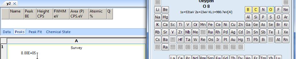
5 Peak Identification SurveyID - Auto Peak Identification The SurveyID provides automatic XPS peak identification and quantification from monochromatic survey spectra. This option is designed to operate on survey spectra including a range of at least ev Binding Energy (XPS spectra) with a step size of 1eV. A smaller energy range or different step size may be used but are not recommended, since certain elements may not be correctly identified. The spectrum will be analysed and only the major peak of each element added. An optimum background position for the peak is also determined. There may be peaks visible ibl on the spectrum which h are not labeled l but all peaks in the spectrum are included in the identification process. The user may choose to use the Manual Peak ID to see the positions of all peaks for a particular element. The background start and end positions are optimized and the selection of a Smart background is recommended. 5

6 Survey ID - Preferences Preferences The recommended Peak database library is ChemState.mdb and use of ALSCOF library. There are two preferences found in Processing Preferences...Analysis...Survey ID. Exclude Highly Radioactive Elements This should usually be checked ON and this reduces the probability of incorrect peak identification. Only users working with radioactive materials should need to change this preference. Show other peaks This option determines if all peaks are labeled on the spectra. This can be preferable if users are less familiar in interpreting XPS spectra as it will avoid unlabeled peaks. However, on a complex spectrum it may result in many labels 6

7 Survey ID Limitations Survey Spectra are not as well resolved as narrow scan data so Peak Area will have uncertainty Quantification from Survey and from narrow scans will probably be different: The current algorithm may not correctly identify peaks when overlaps occur see ESP! If survey range not large enough, algorithm may not find high binding energy peaks (As2p1=1381eV) Name Atomic % Atomic % Survey Narrow Scan N1s O1s C1s B1s

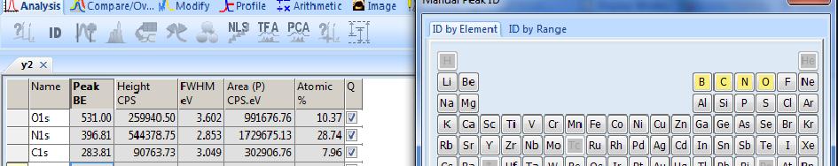
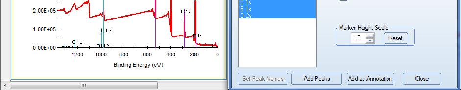
8 Manual Peak ID ID by Element The Periodic Table is used to select elements and show the position of peaks. This can be used to see if there is a good match between the observed spectrum and expected elements. Elements can be selected and deselected using left mouse click. The Peak List shows the details of the peaks displayed for the selected element. Multiple elements may be selected and the Peak List is populated for a given element by click right on the element. The height of the markers in the spectrum display is proportional to the relative sensitivity factors. Filtering of the displayed peaks is possible to remove Auger and Chemical States and select which doublet components are displayed. 8

9 9 Manual Peak ID Typical Procedure

10 PEAK ID By Range Manual Peak ID ID by Range 10

11 Notes on Peak ID Element Probability % To remove some of the more unlikely elements from the search, each element has been assigned probability weighting. Elements which it is common to observe in an XPS spectrum (e.g. C, O) have high h weighting factor, while those unlikely l to be observed (e.g. Pu, Cm) have low probability. By changing the Element Probability the number of possible transitions can be reduced. Show Auger Peaks XPS spectra also have X-ray induced Auger peaks. This option allows the library entries to be displayed or removed to reduce the number of transitions. Approximate relative intensity values are included for Auger peaks but the observed spectra may differ depending upon chemical state, X-ray excitation conditions and other factors. Doublet Peak Options XPS peaks from p,d and f orbitals have two components creating a doublet. The option is provided to display both components, or only the major or larger component of the doublet (p3/2, d5/2, f7/2). Some library entries also have a single combined peak without a suffix e.g. Al2p. These are often used when the doublet separation is very small and may not be apparent, especially on survey spectra. 11

12 Notes on Peak ID Show Chemical State Some libraries have chemical state binding energy shift information. This information can be included in the display or excluded. When manually identifying which elements are present can be easier if the chemical state peaks are excluded. This information is usually more useful when analysing spectra acquired at higher energy resolution. (More on Chemical State later!) 12

13 Peak Add - Introduction Although peaks can be added automatically, usually it is better to add manually (or from an existing peak table) 13

14 Peak Add Notes on Backgrounds Linear Background This is a simple subtraction method based on the assumption that the background corresponds to a straight line, between the start and end points of the background. This method is generally acceptable where there is not a large change in the background height, however, when there is a large change in background heights this can lead to relatively large variations in measured peak area as shown below 14

15 Peak Add Notes on Backgrounds Shirley Background The Shirley background is an approximation method for determining the background under an XPS peak One advantage of using the Shirley type background is that the positioning of start and end points is not as critical as for a Linear background. 15

16 Peak Add Notes on Backgrounds Smart Background The Smart background option is the recommended choice for most general use. The Smart background option is based on the Shirley background with the additional constraint that the background should not be of a greater intensity than the actual data at any point in the region. The calculated background is less sensitive to the selection of the background start and end positions. In the case of multilevel data, the effect of changes in chemistry and shifts in peaks positions can make selection of a fixed background position o difficult. This problem is avoided when using the Smart background. 16

17 Peak Add Notes on Backgrounds Tougaard The Tougaard background option is intended to provide an empirical model of the electron energy loss process which is a more accurate description of the physical processes. It is most applicable to removing a background from a wide energy range spectra, such as survey spectra and it is not widely used for general quantification or background subtraction from spectrum regions. The B, C and D values are defined in Tougaard original publications. These typically vary with the general type of material and predefined sets of these constants may be selected from the Mode list. The values may also be edited manually to obtain the required background shape. Y Offset adjusts the low BE / high KE baseline position. This may be used if another peak contributes to the background intensity at that position but that peak is not included in the full Tougaard background calculation. 17

18 Peak Add Notes on Backgrounds Simple The Simple background option measures the complete area between the start and end of the region and below the spectrum. It has limited use as the intensity from other peaks may affect the total intensity measured. As a greater absolute intensity is measured and hence the statistical variability is lowered, it may have some use when repeatability or precision measurements are required, where the elemental composition is not changing significantly. 18

19 Peak Add Notes on Backgrounds Background Average At Start & End This control defines the range of data used to define the start and end intensities of the background. Applying ppy a range at the start and end of peak definition will improve the accuracy of the peak area measurement. This is particularly important when using multilevel data where the peak definition maybe defined on a single level, but other levels in the data space may have a higher noise level and cause the background to be calculated from a single noise spike. The typical recommended value is 0.5 to 1eV. 19

20 Quantification As indicated earlier Peak Area definition is important to ensure reliable quantification. Uncertainties in peak area have a direct influence on the accuracy of any quantification data. When data is quantified, the peak areas are measured, suitable sensitivity factors are applied to the data and corrections for the instrument transmission function and energy compensation factor (ECF) are made. The standard quantification library data provide a good first approximation quantification but in some cases more accurate ate results may be obtained with the use of standards, relevant to the particular analysis being performed. It is assumed that the depth distribution of all the elements is homogenous. This is often not true (e.g. an overlayer of carbon is often present) but this method provides a simple and consistent first approximation. Quantification of XPS data is a complex subject and to calculate the composition in more detail typically requires a number of assumptions to be made about the sample; effectively you need to know what the sample is before you quantify and this is where standards have an important function 20

21 Quantification The intensity of a peak is related in some way to the number of atoms that generate that peak e.g. I A N A Where I A is the intensity of a peak and N A is the number of atoms of element A Each transition (e.g. C1s, Al2p, Si2s) has it s own probability of occurring - referred to a sensitivity factor and are obtained from libraries. These are generally referred to the Scofield or Wagner libraries e.g. I A = NF.N A (N A =I A /NF) where NF is some kind of normalisation factor, which includes terms for the efficiency (transmission) of the analyser at different kinetic energies, electron mean free path ( ) and the Sensitivity factor 21

22 Quantification Although people use the numbers there are several sources of uncertainty in the result - These can be due to: Determination of the peak intensity? How do you measure a peak area, where do you start from and to, what do you include, what shape background etc Accuracy of Sensitivity Peak Libraries? Different libraries give different results - which is right? Accuracy of the Transmission Function? How well defined is the function for a particular instrument Other Factors include determination of, structure of the surface (layers, islands etc) XPS is good for quantification on a relative scale - comparing similar samples, consistent tmeasurement and ddata treatment t tand dlooking for trends But absolute numbers have a great deal of uncertainty due to above 22

23 Quantification Name Start Peak End Area (P) Area (N) Atomic Peak Q SF TXFN Backgnd BE BE BE CPS.eV % Type (Scofield) B1s Standard Smart C1s Standard Smart N1s Standard Smart O1s Standard Smart Typical Spectra defined Peak Area calculated by software after removal of background (Smart) Effect of peak definition? How is Area (N) calculated? 23

24 Quantification Peak Definition Name Start Peak End Area (P) Area (N) Atomic Peak Q SF TXFN Backgnd BE BE BE CPS.eV % Type (Scofield) B1s Standard Smart C1s Standard Smart N1s Standard Smart O1s Standard Smart Name Start Peak End Area (P) Area (N) Atomic Peak Q SF TXFN Backgnd BE BE BE CPS.eV % Type (Scofield) B1s Standard Smart C1s Standard Smart N1s Standard Smart O1s Standard Smart Small changes in peak definition can effect quantification 24

25 Quantification Area Normalization Name Start Peak End Area (P) Area (N) Atomic Peak Q SF TXFN Backgnd BE BE BE CPS.eV % Type (Scofield) B1s Standard Smart C1s Standard Smart N1s Standard Smart O1s Standard Smart Peak karea Normalization The Peak Area is corrected for the total dwell time per channel, number of scans and energy channel width. Normalised Peak Area = Peak Area / (SF * TXFN * ECF) SF = sensitivity factor TXFN = transmission function ECF = energy compensation factor 25

26 Quantification Sensitivity Factors Name Start Peak End Area (P) Area (N) Atomic Peak Q SF TXFN Backgnd BE BE BE CPS.eV % Type (Scofield) B1s Standard Smart C1s Standard Smart N1s Standard Smart O1s Standard Smart Quantification Libraries i A number of libraries are supplied as standard with the Avantage data system. These are derived from sensitivity factors generated by Wagner and Scofield. The Scofield sensitivity factors are theoretically derived from the photo-ionisation probabilities The Wagner values were determined empirically from a large number of compounds in the early 1980s. The actual libraries have been optimised for the appropriate X-ray anode, e.g. MGWAGNER, ALSCOF etc. 26

27 Quantification Sensitivity Factors Name Start Peak End Area (P) Area (N) Atomic Peak Q SF TXFN Backgnd BE BE BE CPS.eV % Type (Scofield) B1s Standard Smart C1s Standard Smart N1s Standard Smart O1s Standard Smart Two libraries are used but they have to be used in slightly different ways Scofield -A theoretical sensitivity factor data base, based on C1s = 1 (i.e. A calculation which gives a number relating to the number of photoelectrons generated by a number of photons hitting the sample) For this we need to add in a term to account for the depth of analysis (i.e. and is generally KE 0.6 or using the TPP-2M method) Wagner -An empirical sensitivity factor data base, based on F1s = 1 (i.e. Real measurements done on an instrument on a large number of known compounds and working out relative sensitivity factors). For this we need to add in a term to correct for the fact this was generated on a different type of analyser (A CMA rather than our HSA). This is done by multiplying by the KE of the peak used. (The term is already included in the analysis) Both libraries can be used - but different results on the same set of data may be obtained!! 27

28 Quantification ECF - energy compensation factor Name Peak BE Area (P) CPS.eV Area (N) Atomic % B1s C1s N1s O1s The energy compensation factor is applied depending on library being used. The Wagner factors have assumed an instrument transmission function of KE -1. The inelastic mean free path (IMFP) term is effectively included within the sensitivity factor. For Scofield a choice of a simple KE n where generally n=0.6, or the TPP-2M method is required. In the Peak Table the Area (N) indicates which method has been used The selection is set in the Peak Table Property page. 28

29 Quantification TPP-2M energy compensation factor Name Peak BE Area (P) CPS.eV Area (N) Atomic % B1s C1s N1s O1s What is TPP-2M? An alternative to using the KE 0.6 value is to use an average value as derived from the Tanuma, Powell, Penn 2 Method (TPP-2M) [S.Tanuma, C.J.Powell and D.R.Penn - Surface and Interface Analysis, Vol 21, (1993)]. This is a more detailed approach to calculating Inelastic Mean Free Paths (IMFP) 29

30 Quantification TPP-2M energy compensation factor The full expression contains several terms associated with the physical properties of the surface many of which cannot be determined by XPS analysis. The above expression can be simplified to a more general approach using average matrix values: (Briggs & Grant, p363, eqns 53-55) and assuming E g = 0 Where N V = 4.684, = and M =

31 Quantification TPP-2M energy compensation factor 3.5 Comparison of KE 0.6 and TPP- 2M methods Electron Mean Free Pa ath (nm) Note slight difference in compensation at different kinetic energies This would lead to slight TPP differences in quantification KE Pownumbers Thus care required that a consistent approach is used for any quantification Kinetic Energy i.e. Scofield and TPP-2m (recommended) Or Scofield and KE

32 Quantification Summary Name Peak BE Area (N) TPP 2M Atomic % B1s C1s N1s O1s Name Peak BE Area (N) KE 0.6 Atomic % B1s C1s N1s O1s Comparison of KE 0.6 and TPP-2M methods using the same data Thus care required that a consistent approach is used for any quantification including survey/narrow scan, peak definition and choice of library i.e. Scofield and TPP-2M (recommended) Or Scofield and KE Narrow TPP-2M (full N range) Narrow TPP-2M Narrow KE 0.6 Survey TPP-2M B1s C1s N1s O1s

33 Chemical State One of the major advantages of XPS analysis is the ability to determine the chemical state of elements found on the surface. Avantage can provide an estimate of possible chemical state using the database and the Chemical State Assessment tool Chemical Composition of Sample Spectral Region Details C-O-C C1s *C-O-C* O1s C-O*-C carbon C1s C-C or C-H O-C=O C1s O-C*=O O1s O-C=O* O 33

34 Chemical State Knowledge Base Using the Knowledge base will also provide useful information associated with elements 34

35 Chemical State Knowledge Base Using the Knowledge base will also provide standard data associated with chemical state 35

36 Charge Shift Charge shift is used to set the correct energy scale for a series of spectra, based on setting the peak position to a defined position. The most common calibration peak used is C1s = 284.8eV, although other values may also be preferred. In normal operation, all of the data should be shifted by the same amount. The simplest way to do this is to select all of the data before opening the Charge Shift dialog. Select the grid cells containing the spectra to be shifted. If only spectra are displayed and they all have the same axes (other than energy), you may also use the cell heading at the upper left corner of the processing grid. Alternatively use <Ctrl>(left mouse click) to select / deselect grid cells. 36

37 Charge Shift Here the C1s peak is at 280eV 37

38 Charge Shift Shift to peak from database 284.8eV 38

39 Peak Fitting There is a certain amount of confusion in what parameters are acceptable or otherwise when undertaking the peak fitting. Peak fitting is a very complex subject and frequently there is no correct answer, and sometimes the approach is the least wrong rather than the most right! To start with: What are we doing with peak fitting? We are applying synthetic ti peaks using a mixture of Gaussian and Lorentzian shapes to try to fit as close as possible the data obtained from an XPS experiment. Without going into the details too much, the XPS peak can be described as a convolution (or mixture) of Gaussian and Lorentzian functions, or the L/G mix. The Gaussian describes the measurement process (instrumental and source) while the Lorentzian models the natural or intrinsic broadening 39

40 Peak Fitting The classic approach (i.e. simplified) of how the width ( E) or shape of a photoelectron peak is determined is shown below: E 2 E 2 source+ E 2 intrinsic+ E 2 instrument E 2 source is the width and shape of the x-ray source so will be relatively narrow when using a monochromator but somewhat broader if using unmonochromated x-ray sources. E 2 intrinsic is the width and shape of the natural transition being examined. For the first approximation the shape (L/G mix) can be regarded as constant, while the widths should be similar, but will vary according to chemical state (e.g. oxide peaks are generally wider than metallic peaks) E 2 instrument is the width and shape induced by the instrument and the biggest factor here would be the effect of pass energy. 40

41 Peak Fitting What this means in practice is that over a narrow range of energies (i.e. a narrow scan spectrum) the L/G mix should be the same for the same transition in this case the C1s transition. However the widths can vary according to the chemical state. It is important t to note that t the * *bonding (or Sat in the example) is not a C1s transition but is an energy loss feature from the C-C C peak so would not have the same L/G mixture. 41

42 Peak Fitting Example The C1s region from a PET sample is shown. Firstly define the peak as normal. Using the Peak Fit icon peaks can be defined on the spectrum. 42

43 Peak Fitting The mathematical process is using defined model peak shapes The shape parameters for the peak (height, width, G/L function etc.) are automatically varied until the best fit to the observed spectrum is achieved. Constraints and linking of peaks can be applied so that t the results of the fitting process remain physically and CHEMICALLY realistic. Adding single peaks allow the population of Peak Fit table. Clicking on the Fit Peaks tab, the first pass fitting can be undertaken by clicking on the Fit This Level. 43

44 Peak Fitting Adding single peaks allow the population of Peak Fit table. Clicking on the Fit Peaks tab, the first pass fitting can be undertaken by clicking on the Fit This Level. 44

45 Peak Fitting At the moment the default peak fit parameters have been used. This means that for example the L/G mix is fixed at 30%. At this point it is worth labelling the peaks as shown. Although this first pass fit looks OK, on closer inspection there is a mis-match match on the C-C peak leading edge. This is due to the mixing of the Gaussian and Lorentzian shapes previously discussed 45

46 Peak Fitting To solve this issue the constraints need to be altered so that the L/G mixture is allowed to vary to obtain the best fit. The existing constraint needs to be removed and then new constraints applied. This constraint should be applied to the other photoelectron peaks in the region (The C-O and O-C=O peaks but not the Sat peak). In this case simply typing in A will result in the constraints shown. After the second peak fit the result is as shown. The fitting of the leading edge of the C-C peak is better as shown. 46

47 Peak Fitting Additional Functionality Doublet peaks may be added using the Add Doublet button, which is enabled when the region name is one where a doublet may be expected - a p, d or f core level. For example a region named as Cu2p will allow addition of a doublet but a region named Si2s will not. The separation is calculated l from the peak library and the relative intensities of the two doublets are set from the relative sensitivity factors in the peak library. Constraints are also set for these parameters. 47

48 Peak Fitting Asymmetric Peaks Asymmetric peak shapes may sometimes be useful for fitting spectra of electrical conductors (metals, carbon fibres, some nitrides and carbides). This is applying an exponent to the lower binding edge of the peak Using symmetric peaks on iron produces an unsatisfactory t result Allowing Tail mix, and tail exponents to vary a better fit can be obtained. Peak fitting asymmetric peaks are difficult and there are many different approaches that can be used 48

49 Peak Fitting Constraints Peak Fitting Constraints The peak fit parameters for each peak may be constrained to restrict the range in which the parameter may be adjusted during the automatic peak fitting process. This can prevent the peaks becoming unreasonably narrow or wide or to input known chemical information e.g. spin orbit doublet separation or intensity ratio. The symbols used in the Peak Fit Table are Vl Value is constrained din a range Value is linked to the value of another peak. The Reference of the linked peak is used to define the link. 49

50 Peak Fitting Constraints Constraint A+2.3 Details Link position relative to another peak Use Ref. of other peak, arithmetic operator and value. A*1.5 Use Ref. of other peak, arithmetic operator and value. link the width of peaks to be related to another peak A Sets the value to the current value of the Ref. peak A? Link a peak to the current value of another peak and automatically calculate the parameter A (+ 0.1) Linked Range Link a peak to the current value of another peak with a Range of the link value A (+ 0.1) 1)will set the position to be the value of A +1.5eV but will allow the parameter to vary between 1.4 and 1.6eV A * 1.5 (+ 10%) will set the value to be the value of A * 1.5 but will allow the parameter to vary between 1.35 and Fix a peak at its current value Click on the Fix Constraint icon Enter the word fixed or f in the constraint for the peak The following methods may be used to set the absolute range of a parameter whatever method is used to enter the values, the absolute values are always displayed :2.5 value1 : value2 Fix a parameter between two values Fix a parameter within a range of the current value + value will constrain the parameter to move within a range of +0.2 to 0.2 of the start value. +0.1, 0.2 +value1, value2 Fix a parameter within a range of the current value +0.1, 0.2 will constrain the parameter to move within a range of +0.1 to 0.2 of the start value. Remove a Constraint Select the constraint to be cleared and press the Remove Constraint icon or Click in the constraint cell and delete the text entry All constraints in one or more columns or rows may be removed by selecting multiple columns or rows andpressing the icon. 50

51 Peak Fitting Other Terms Peak Fitting Algorithm A selection of two fitting algorithms is provided - the Simplex and the Powell optimisation. The Simplex algorithm can find false minima and restarting a fit can then result in a better fit. The Powell method appears to be more robust and less likely to find a false minimum but can be slower. Other Peak Shape Functions In addition to the usual recommended default option of Gaussian Lorentzian (G-L) product function, it is also possible to select either G-L LSum function or a GL G-L Convolution function. The Convolution function involves more calculations and is slightly slower. In some cases, an alternative function may give an improved peak fit but there is no generally consistent physical or empirical model. Abbe Criterion The Abbe Criterion examines the residuals - the difference between the actual data and the fitted data - to determine the statistical "randomness". A good fit model should have residuals that only show statistical noise. 51

52 Peak Fitting Multilevel & Propagate Constraints Peak Fit at every level of multilevel data such as depth profiles is possible. The constraints may be copied or propagated to every level. l In most cases, the constraints will be the same for every level in the profile although it is possible to manually edit the constraints for any level within the profile. To propagate the constraints, click right in the peak table and select Propagate Selected Values / Constraints The dialog allows selection of the range of levels for propagation of the constraints. Buttons allow propagation of either Values in the Peak Fit Table Constraints in the Peak Fit Table Both Values and Constraints 52

53 Peak Table Profile The Peak Table Profile processing plug-in will quantify data across the whole of a multidimensional dataspace. This may be a depth profile, angle profile, iteration, ti linescan, area scan. A Peak Table must have been defined A dialog is displayed allowing selection of the profile type to be produced If more than one profile is selected, then the profiles are added to a single dataspace After pressing OK, a new dataspace is created. The NavBar can be used to step through each of the selected profiles. 53

54 Peak Table Profile The example is aluminium foil 8.00E+04 o1s 6.00E+04 c1s In some cases, the output data may be displayed d in an unfamiliar form, particularly l with multidimensional data but it may changed using the Display Properties and Axis Properties. Cou unts / s 6.00E E E E+00 AR Normalised Area is used for some angle 4.00E+04 resolved ARXPS processing. This is calculated 3.00E+04 in the same way as atomic % except that the 2.00E+04 attenuation length term is not included in the 1.00E+04 calculations. This is important for use with the Multiple Overlayer Calculator and ARProcess 0.00E+00 programs where the attenuation lengths are explicitly calculated. Counts / s O1s Binding Energy (ev) al2p Binding Energy (ev) Cou unts / s Peak Area CPS.eV 4.00E E E E E E Binding Energy (ev) Profiles O1s C1s Al2p 0.00E Etch Level Profiles = Peak Area CPS.eV Name Peak Height FWHM Area (P) Atomic Q BE CPS ev CPS.eV % O1s Y C1s Y Al2p Y 54

55 Peak Table Profile Use the Axis Properties to set the range of data to view and use the Display Mode to choose the way to display the data. Time to Depth Conversion Depth profile data is acquired and stored with an axis measured in etch time. If the sputter rate is known, then as a first approximation, the etch depth may be calculated. The Time to Depth conversion may be applied either to the raw spectra data, or more usually to the generated Peak Table Profile. This is usually better because it allows all of the peaks in the profile to have the same depth scale applied.. 55

56 Peak Table Profile The previous data was acquired using only elemental data, i.e. Al, C and O Using peak fitting the peak table can be generated with fitting at every level of the Al2p region providing quantified data for Al metal and Al oxide. 56

57 Peak Table Profile The fitted Al2p3 and Al2p1 from the metallic portion can be combined using Combine Selected peak tool and the profile generated as before. This profile shows good agreement with expected profile i.e. Oxygen and Al Oxide follow the same profile. 57

58 Target Factor Analysis - TFA The ideal situation would be to peak fit at every level in a multi-level data set to obtain more accurate quantification data. However, pure metallic components are often not a simple G-L peak shape but will have asymmetry which is difficult to fit. The situation is mirrored in Auger spectra where the peak shapes are complex. The two tools TFA and NLLSF enable the user to obtain useful information from multilevel data especially where complex peak shapes are obtained. These are mathematical techniques that extract common factors from a set of data, and then apply these components to extract information about the samples composition. This is usually depth profile data but could also be an multilevel data. TFA assumes that the profile data is composed of a linear sum of common spectral components. TFA can only determine the number of components but cannot identify them. 58

59 Target Factor Analysis - TFA The most significant levels in the profile are chosen by the TFA and then each level of the profile is fitted with these spectra using a linear combination of these components. The goodness of fit is then calculated at each level and is compared with the user defined Signal:Noise (S:N) limit. If any level is not fitted satisfactorily then that level is added as a component and the process continues with additional spectra being added until every level is fitted to better than the S:N Limit. The number of spectra required reflects the number of significant components in the profile. Note that the spectra used as components may not be a pure reference spectra. TFA provides a Best Guess at the principal components in multi-level data and if the principal components are pure references the result will accurately reflect the change of these components in multi-level data. When the TFA has determined the principal components it automatically runs a Linear Least Squares Fitting (LLSF) of the data with the components.. 59

60 Target Factor Analysis TFA, LLSF and NLLSF Linear Least Squares Fitting (LLSF) makes the assumption that the profile data are composed of a linear sum of component spectra and the peak positions do not change These component spectra may be defined by TFA or by the user. The user defined options include previously acquired spectra, synthetic peaks from a peak fitting or levels within the profile data. For example in sputtering through silicon oxide on silicon, a reference spectrum for the silicon oxide may be taken from the oxide layer and a reference spectrum for the elemental silicon from one of the levels in the substrate after sputtering. Non-Linear Least Squares Fitting (NLLSF) assumes that the profile data is composed of a sum of component spectra but that the peak positions may vary in the depth profile e.g. due to charging. In NLLSF, the reference spectra are determined as before, but at every level in the profile, the peak positions are adjusted to give the mathematical best fit. 60

61 Target Factor Analysis TFA Clicking on the TFA icon will open the TFA dialog Select the Signal to noise ratio A good default value is 3. A lower number will find more components; a higher number will find fewer components Press Start TFA The dialog displays a progress bar and the output data is displayed in a new process grid document. 61

62 Target Factor Analysis TFA TFA Levels Principal factors determined using the S:N. Pure metallic Al (level 34) and aluminium with a thin oxide (level 4). Level 4 is not a pure factor, but TFA has provided the most significant factors TFA Profiles This is an intensity profile of each of the TFA Levels. The oxide rises at the start then drops. The metallic component is low at the start t but rises as the etching continues TFA Residual The TFA residual display shows the difference between sum of factors at each level and original data. A good fit, would be random noise. TFA Chi-square Profile This goodness of fit at each level, 62

63 Target Factor Analysis TFA TFA Eigen Spectra This display shows the result of a matrix analysis of the data from which the effects of noise can be discounted from the final result. As can be noted in the display, this analysis approximated well to two components that are similar to a pure metallic Al state and a pure Al oxide state. 63

64 Target Factor Analysis TFA The Accept button will write the TFA peaks /TFA Levels back to the original processing document as LS Fitted peaks. Peaks can be renamed in the Peak Table using more descriptive names. A Peak Table Profile can then be used to generate a profile for all included elements and factors. The TFA data and sum of TFA factors at each level may then be viewed in the original processing document. 64

65 Linear and Non-Linear Least Squares Fitting In many ways NLLSF is an extension of Peak Fitting and TFA. The advantage that NLLSF has over normal peak fitting is that real peak shapes compared with G/L mixtures can be applied to sets of data. TFA supplies only a linear combination of real peak shapes, so peaks that move during the analysis will not be accurately determined. Reference components can be obtained from various sources, and in comination References within the Multi-Level Data Set The easiest method is to use reference spectra from within the multi level l data set. References from Standard Data If a pure component spectrum exists it is possible to define this as a reference component. References from Derived Data In this case synthetic components that have been obtained by peak fitting can be used. 65

66 Linear and Non-Linear Least Squares Fitting Example using Synthetic (Al oxide) and Pure Reference (Al metal) The Synthetic Peak is from the peak fit done previously, the metallic from level 43 of the profile. These spectra are opened in a separate processing document compared to the original data. 66

67 Linear and Non-Linear Least Squares Fitting Select the Al2p depth profile region in the original processing document, then click on the NLS button to open up the dialog. If there are references already present in the dialog these should be deleted using the delete button. Select the processing document containing the external reference spectra Select the reference spectra and click Add button in the NLLSF dialog. This will add each reference spectrum to the dialog. The name can be changed for reference. 67

68 Linear and Non-Linear Least Squares Fitting Select the processing document containing the synthetic reference spectra Select the reference spectra in the peak table and click Add button in the NLLSF dialog. This will add this reference spectrum to the dialog and again the name can be changed for reference. 68

69 Linear and Non-Linear Least Squares Fitting Shifts parameters are set to the correct values (1eV and not linked) (if set to 0, this will be LLSF!) Clicking on the Start NLLSF button will open the NLLSF processing grid document. Clicking on the Accept button will transfer the data to the original Processing view. 69

70 Linear and Non-Linear Least Squares Fitting The original processing view will now show in the peak table two components for the Al2p region: Al2p Oxide which is derived from the peak fit of the region and Al2p Metallic which is a pure metallic component from within the multilevel l set. The profile can be generated using the Peak Table Profile 70

71 Spectrum Comparison - Lightbox Light Box Compare The recommended way to compare spectra is to use the Light Box Compare feature. Light Box Compare allows similar spectra to be overlaid and then rescaled and shifted to obtain a visual comparison. The tool is intended to provide a visual comparison and because spectra may be scaled or shifted, the scales on the axes should be treated only as arbitrary values. Select the spectra to be overlayed using <Ctrl> left click in a grid cell. For multilevel data, first select the level you want using the NavBar. If spectra from more than one processing document are required, select a spectrum from the first processing document and then add other spectra using the Light Box Compare dialog. The same method can be used to select more than one spectrum from a multilevel dataspace. The spectra to be compared should have the same energy step size. A new processing grid titled Compare #1 is created. 71

72 72 Spectrum Comparison - Lightbox

73 Energy Deconvolution Energy Deconvolution removes the effect of analyser broadening. This enables use of a data acquired at a high pass energy to be transformed to appear as though it had been acquired at a lower pass energy. This enables higher energy resolution data to be obtained in a shorter acquisition time because of the higher sensitivity at higher pass energy. This can be particularly useful when using snapshot spectra on K-Alpha and Theta Probe instruments. This is achieved by use of a point spread function (PSF) to represent the broadening that a single zero width energy peak would experience. For K-Alpha, the PSF is acquired and calibrated using the Spectrum PSF procedure, however for ESCALABS and ThetaProbes a calibration procedure is required usually on silver. It is important that the instrument is correctly set up and it is recommended that the calibration procedure be repeated after maintenance activities. 73

74 Energy Deconvolution Deconvolution of an Acquired Spectrum After calibration has been performed, the PSF values can be used to correct a spectrum. Load the spectrum and select Energy Deconvolution Select Old Registry Select the Pass Energy to Deconvolve from and to from the list of available PSF calibration values Select the Effective Pass Energy for Deconvolution and press Apply. Select either Deconvolve Display Level or Deconvolve All Levels for multi level data. The effect can be seen in the process grid but the changes are not finalised until the Accept button is pressed, allowing selection of different parameters. 74

75 Energy Deconvolution To protect samples from prolonged exposure to X- rays, data can be collected initially at high PE. C1s Scan 150eV deconvoluted 2 Scans, 19.1 s, 400µm, 0.10 ev 1.00E+05 C1s Scan 20eV 20 Scans, 3 m 11.0 s, 400µm, 0.10 ev 4000 This results in data with good S/N, but poorer resolution. Deconvolution can then be applied to give high resolution spectra. Data collected at 150eV PE and 20eV PE are compared here Counts / s 8.00E E E E E Binding Energy (ev) Counts / s Binding Energy (ev)

76 Energy Deconvolution Further reductions in collection time can be achieved using snapshot acquisition mode C1s Snap Frames, 5.0 s, 400µm, 128 chans Here 150eV pass energy was used to give ~20eV dispersion across the detector 300 Counts / s A 128 point (one point per channel) snapshot spectrum can then be collected without the need to change the analyser energy. The acquisition time for a typical snapshot spectrum is 1s. 700 This is ideal for mapping and depth profiling 600 applications where large numbers of spectra are 500 being acquired Binding Energy (ev) C1s Snap Frames, 5.0 s, 400µm, 128 chans. 900 Counts / s Decon volution Binding Energy (ev) 76

77 Concatenate Depth Profile Introduction This is a separate utility that allows data acquired in multiple depth profiles to be combined into a single depth profile. C:\Program Files\Thermo\Avantage\bin\ConcatenateDepthProfiles.exe. This may be useful if a profile was stopped or had too few etch levels to reach the required interface. Although it may also be used if different etch conditions are used, the user should be aware that the sputter rate in different operating modes may be significantly different, especially if using Cluster modes for MAGCIS ion gun. Restrictions All data must have the same region name, data acquisition ranges, pass energy, step size and acquisition times and there must be only the same set of regions in each section of the depth profile. 77

78 Combine Points Introduction This is a separate utility that allows data acquired as separate points to be combined into a single set of dataspaces. This allows use of multi-level features such as Peak Table Profile, Peak Fitting at every level, Non-linear least squares fitting (NLLSF). Restrictions All points must have the same region name, data acquisition ranges, pass energy, step size and acquisition times and there must be only the same set of regions at each point. Operation Ensure that all of the data to be combined is located under the same parent folder. Data may have been acquired in the same experiment as shown. Alternatively, ti l the individual id data folders could have been manually copied from multiple experiments into a new folder. 78

79 Combine Points Operation Open Windows Explorer and select the C:\Program Files\Thermo\Avantage\bin folder and run the CombineMultiplePointsIntoMultiPoint.exe program. Select the parent folder that contains the sub-folders with data from the separate points and Press OK A second folder dialog is displayed to allow selection of the location of the output data. This defaults to the original folder. 79

80 Combine Points A dialog identifies the number of.vgd files and the main window displays the original filenames. A set of new.vgd files are created with the suffix _Combined in the selected folder. The data can then be loaded normally in Avantage. Data can be navigated using the NavBar and the original X and Y coordinates will be displayed. Peaks may be added, peak fitting or other multilevel processing (PCA, TFA, NLLSF) and Peak Table Profiles generated as for any multilevel l data set. 80

81 ESP The New and Improved Survey ID The current Survey ID sometimes does not find peaks so an improved version will shortly be available The example here is as received Boron with an oxide layer Note the peak at about 190eV has not been labelled after using Survey ID The minor peaks are shown and the annotation is complicated To improve this a new tool (ESP) has been developed with added functionality 81

82 ESP The New and Improved Survey ID The tool undertakes a more rigorous treatment of the data, and will produce more accurate identification 82

83 ESP The New and Improved Survey ID Data is classified Green high confidence, Yellow medium confidence, Pink low confidence and blank if not found 83

84 ESP The New and Improved Survey ID Extra peak labels can be active or not active 84

85 ESP The New and Improved Survey ID Confidence factor enables educated decisions whether a peak is really present e.g. Boron high confidence 85

86 ESP The New and Improved Survey ID Confidence factor enables educated decisions whether a peak is really present e.g. Magnesium medium confidence but is it really there? 86

87 ESP The New and Improved Survey ID Confidence factor enables educated decisions whether a peak is really present e.g. Aluminium low confidence but maybe it really there use show markers 87

88 ESP The New and Improved Survey ID Simple click and medium confidence peaks can be removed 88

89 ESP The New and Improved Survey ID Magnesium in this case was B KL1 Auger transition Once ID has proceeded the peaks determined can be added to the experiment tree automatically ti using the Add Regions to Experiment function 89

90 Questions? 90