Laser-induced plasma on polymeric materials and applications for the discrimination and identification of plastics

Transcription

1 Laser-induced plasma on polymeric materials and applications for the discrimination and identification of plastics Myriam Boueri To cite this version: Myriam Boueri. Laser-induced plasma on polymeric materials and applications for the discrimination and identification of plastics. Other [cond-mat.other]. Université Claude Bernard - Lyon I, English. <NNT : 2010LYO10207>. <tel > HAL Id: tel Submitted on 19 Sep 2012 HAL is a multi-disciplinary open access archive for the deposit and dissemination of scientific research documents, whether they are published or not. The documents may come from teaching and research institutions in France or abroad, or from public or private research centers. L archive ouverte pluridisciplinaire HAL, est destinée au dépôt et à la diffusion de documents scientifiques de niveau recherche, publiés ou non, émanant des établissements d enseignement et de recherche français ou étrangers, des laboratoires publics ou privés.

2 N d ordre Année 2010 THESE DE L UNIVERSITE DE LYON Délivrée par L UNIVERSITE CLAUDE BERNARD LYON 1 ECOLE DOCTORALE DIPLOME DE DOCTORAT (arrêté du 7 août 2006) soutenue publiquement le 18 octobre 2010 par Myriam BOUERI TITRE: Laser-induced plasma on polymeric materials and applications for the discrimination and identification of plastics Directeur de thèse : Professeur Jin YU JURY : M. Bruno BOUSQUET Rapporteur M. Alexandre SEMEROK Rapporteur Mme. Nicole GILON-DELEPINE Examinateur M. Jörg HERMANN Examinateur M. Frédéric PELASCINI Examinateur M. Pierre TOULHOAT Examinateur M. Vincent MOTTO-ROS Examinateur M. Jin YU Directeur

3

4 N d ordre Année 2010 THESE DE L UNIVERSITE DE LYON Délivrée par L UNIVERSITE CLAUDE BERNARD LYON 1 ECOLE DOCTORALE DIPLOME DE DOCTORAT (arrêté du 7 août 2006) soutenue publiquement le 18 octobre 2010 par Myriam BOUERI TITRE: Laser-induced plasma on polymeric materials and applications for the discrimination and identification of plastics Directeur de thèse : Professeur Jin YU JURY : M. Bruno BOUSQUET Rapporteur M. Alexandre SEMEROK Rapporteur Mme. Nicole GILON-DELEPINE Examinateur M. Jörg HERMANN Examinateur M. Frédéric PELASCINI Examinateur M. Pierre TOULHOAT Examinateur M. Vincent MOTTO-ROS Examinateur M. Jin YU Directeur

5

6

7

8 Résumé La spectrométrie de plasma induit par laser, plus connue sous le nom de LIBS (l acronyme du terme en anglais Laser-Induced Breakdown Spectroscopy) est une technique analytique qui permet la détection de l ensemble des éléments du tableau périodique avec des limites de détection de l ordre du ppm et ceci sur tous types d échantillons qu ils soient liquides, solides ou gazeux. Sa simplicité de mise en œuvre, sa rapidité et sa versatilité en font une technique très attractive avec un fort potentiel en termes d applications que ce soit pour le contrôle en ligne, l environnement ou l exploration spatiale. Son point faible reste cependant son manque de fiabilité dans l analyse quantitative, en particulier lors de l étude d échantillons hétérogènes ou de matrices complexes telles que les matrices organiques. Ce travail de thèse propose une étude des propriétés des plasmas induit par laser sur différentes familles de polymères. Une étude du plasma au temps court (~ns) par ombroscopie est tout d abord présentée, ceci pour différents paramètres expérimentaux (énergie laser, durée d impulsion, longueur d onde). Un diagnostic complet du plasma par spectrométrie d émission est ensuite détaillé pour différents délais de détection et montre que la mesure des températures des différentes espèces du plasma (atomique, ionique et moléculaire) permet de vérifier, dans certaines conditions, les hypothèses d homogénéité et de l équilibre thermodynamique local. Ceci permet alors la mise en place de procédures quantitatives telles que la méthode dite sans calibration (calibration free LIBS) tout en optimisant le rapport signal sur bruit de la mesure LIBS. Dans nos expériences cette optimisation est mise à profit pour l identification de différentes familles de polymères en utilisant, pour le traitement des données de la spectroscopie LIBS, la méthode chimiométrique des réseaux de neurones artificiels. Les résultats obtenus, très prometteurs, permettent d envisager l utilisation de la LIBS pour l identification en temps réel des matières plastiques sur chaine de tri. Par ailleurs et de manière plus générale, ce travail pourrait constituer une base solide pour aller étudier d autres matériaux organiques plus complexes tels que des tissus biologiques.

9

10 Abstract Laser-Induced Breakdown Spectroscopy (LIBS) is an analytical technique that has the potential to detect all the elements present in the periodic table. The limit of detection can go below a few ppm and this regardless of the physical phase of the analyzed sample (solid, liquid or gas). Its simplicity of use, its rapidity to get results and its versatility provide this technique with attractive features. The technique is currently developed for applications in a large number of domains such as online control, spatial explorations and the environment. However the weakness of the LIBS technique, compared to other more conventional ones, is still its difficulty in providing reliable quantitative results, especially for inhomogeneous and complex matrix such as organic or biological materials. The work presented in this thesis includes a study of the properties of plasma induced from different organic materials. First, a study of the plasma induced on the surface of a Nylon sample at short time delays (~ns) was carried out using the time-resolved shadowgraph technique for different experimental parameters (laser energy, pulse duration, wavelength). Then, a complete diagnostics of the plasma was performed using the plasma emission spectroscopy. A detailed analysis of the emission spectra at different detection delays allowed us to determine the evolution of the temperatures of the different species in the plasma (atoms, ions and molecules). The homogeneity and the local thermodynamic equilibrium within the plasma was then experimentally checked and validated. We demonstrated that the optimisation of the signalto-noise ratio and a quantitative procedure, such as the calibration-free LIBS, can be put in place within a properly chosen detection window. In our experiments, such optimised detection configuration was further employed to record LIBS spectra from different families of polymer in order to identify and classify them. For this purpose, the chemometrics procedure of artificial neural networks (ANN) was used to process the recorded LIBS spectroscopic data. The promising results obtained in this thesis makes LIBS stand out as a potentially useful tool for real time identification of plastic materials. Finally, this work can also be considered as a base for the further studies of more complex materials such as biological tissues with LIBS.

11

12 Logic will get you from A to B. Imagination will take you everywhere. Albert Einstein For Momsis, Daddie and little Soussie

13

14 Acknowledgement Wow it s over and there are so many people that need to be thanked and to be honest, these few pages gave me the biggest writers block possible. How to thank ALLLL the people that made this possible? It goes without saying that, even though this thesis was written by me, it would have never been possible to write without the moral support and scientific enrichment that it bathed in. REALLY! So here goes my attempt to put into words what cannot be expressed in words, so please bear with me (and my humour). I would first like to thank my thesis supervisor Jin Yu for giving me the chance to surpass my every limit. You gave me the opportunity to create special memories of all the places visited and people encountered all along this thesis. Thank you for also keeping your sanity during the long nights of corrections when I was surely losing mine. In fact, during the whole period, I watched as you sacrificed countless hours of sleep and put your maximal efforts to get the potential of LIBS out of the lab into the world! No potato or carrot or milk and even plastic sample would be safe! It only comes natural to thank Vincent Motto-Ros for his valuable implication during this thesis. Your energy boosts were not only beneficial for me, but to our whole team. Your patience and teaching methods helped me beyond words, especially during those times when I could see no light at the end of the tunnel. Jin and Vincent, you both make an excellent team, and with your motivation and passion, you will attain the heights and merits of your work. This thesis took place in 3 different laboratories around the world. I thank Christian Bordas, LASIM director for his support and help during difficult situations. It was also a pleasure to meet Rick Russo and Sam Mao during our collaboration with the Berkeley team. Rick, it was a little unreal to have met you in person and I would like to thank you for everything you have made possible for me. Thank you for your constant faith in me. I cannot begin to explain to you how fulfilling it was to work there! Jhanis, Erin, Vassilia, Travis and Dayana: I know I don t stay in touch as much as I would like because I m just really bad at that. I hope you all know how much I enjoyed working with you and even more how privileged I feel to count you as my friends. Thanks to Xianglei, who took time away from his hectic schedule to help me setup my shadowgraph experiments. Lastly, I would like to thank Heping Zeng for his warm welcome in Shanghai. Working with Bai was a great pleasure and I am sure that her hard work will get her very far in life! My most sincere thanks go out to Bruno Bousquet and Alexandre Semerok. Every conference was always in highest of spirits thanks to you two. I still laugh when I think about the night we had dinner and made origami swans in Rome! Alexandre, you witnessed the evolution of my thesis from almost

15 day one, and it was an honour to have you at my jury table. Then there is Jörg! You were there as well from the very beginning. Nothing was too much for you! You were able to juggle science and intellect by day and fun and dancing by night like a pro. Frédéric, you were always such great company and full of lots of useful advice. I hope you can finally see the man in the moon! Thank you Mme. Gilon for allowing us to use your lab for our endless potato experiments. A big thank you to M. Pierre Toulhoat for being the president of my Jury. In fact, it goes without saying, that I had the best jury members one could ever ask for! I think every PhD student can tell you how long 3 years can be. Before it starts you do whatever you can and work however hard you can to finally get that allocation de recherche to be able to do the thesis. Then when you do get it, you start the customary why in the world did I want to do a thesis that bad in the first place?? Everyone around you realises you have become obsessed with your thesis but you well until the last year where you admit this after you work endless hours writing the manuscript up AND even dream about writing it up EVERY night! For the newbies reading this HA HA good luck!! You ll soon understand what awaits you I have no idea how you are going to cope but this is how I did. First, I kept the number to the nearest asylum on speed dial and made sure I was surrounded with people (lots) that enjoy grabbing a pint (or pints depending on the day or week you ve had) of beer nearby. Please note that they cannot just be any kind of people! They need to posses the rare gift of being able to listen to you go on and on (and on and on and on) about how insane your week has been and how you are drowning in work. At LASIM I had a number of very patient and magnificent people that filled out that role better than I could have every wished for. The service informatique Francisco, Sad and Xavier were my secret asylum. Since day one they dealt with my freak outs, break down, rambling, crazy hysterical laughter and eccentricities so bravely that they should be awarded some kind of Purple Heart for surviving the whole ordeal. I love you guys! I have to tell you that the years were filled with doctorate students of very high calibre (please insert the cliché joke not just because I was there here). We created our own little circle of concentrated madness and delirious moments. I hope the Christmas traditional meal and those runs around the parks to help get rid of extra stress (or love handles, whatever excuse you want to use is ok) we worked so hard is still going on. For the more daring ones all I have to say is: Mardi Gras, Monte Cristo and Poker nights!! Thanks to every student and very extra special thanks to Amandine, Bruno (ah Bruno. Je resume toute dans une phrase juste pour toi: Je suis passée par Charpennes pour te dire que ma sœur te kiffe Cecilia, Claire, Cyril, Laure, Marion, Maya, Rami, Vincent and Yara. Ok even more special thanks need to go to Cecilia and Cyril how unfortunately had to share an

16 office with me. Those of you who know me will understand what I m talking about (ne te vexe pas Cyril, je sais que tu mérites encore plus de remerciements vu que tu as été mon mari de boulot. Mais bon, là je suis à la bourre et cette thèse a besoin d être imprimée rapidement donc j'ai dû faire court! Je ne peux plus me cacher dans mes obligations :p). Thanks to Marcus, Framboise, Laurie, Pierre, Julie for the good times especially our lunch special conversations. You cannot come through LASIM without meeting Aurelie, who always made sure I was OK. We were able to share moments of giggles and old fashion girly gossip in a very mature fashion of course n est-ce-pas Aurelie ;) Then one day, out of the blue, came Veronique (a.k.a mon ange gardien) whose presence alone made everything always better. I cannot begin to tell you how important she became to me That s what was always good with us; we understood things without always having to say them out loud. Je sais que tout le monde remercie toujours les femmes de ménages (car sincèrement il faut voir l état de certains bureaux de thesard!!). Mais je tenais à vraiment remercier Marie-Louise pour ses petites surprises de bon matins (si vous avez la chance de les recevoir, vous saurez qu elles ont la magie de garantir que ca va être une très bonne journée!). Thanks to Heather (loved talking to you), Véronique (tes conseils m ont fait beaucoup de bien), Christophe et Jérome. My internship could not have been possible without the help of Estelle (aka Tetelle) and Matthieu. You know when you arrive in a new city and everything just looks the same and you can find your marks and just don t understand how things work and you just desperately need some guidance. Well, Estelle was that for me. Thank you for explaining things over and over again, teaching me ropes, giving me a heads up on what to do (and many times what not to do!). You helped me survive my introduction to LIBS. Matthieu, who became a brilliant scientist and I m sure will continue to excel in everything he does, was Jin s first thesis student. It was not always easy coming after someone that was so talented but it did challenge me and allowed me to give the best that I could. Un grand merci également à Marc N., pour les échanges culturelles ainsi que pour ta patience et ton aide pour faire avancer mes manips. Thanks to Wenqi and Ma Qianli for their good humour and for always keeping a smile on their face no matter what was going on! And Josette wa hen! You re internship with our team was a fresh of breath air! You re hard work and motivation was contagious! You were there until the very last second, coaching me for hours and hours!!! Now, I really believe that I had some kind of favour left over from my past lives, because the gods (or how Josette prefers to say the God) above blessed me with the perfect (not the best or anything close to the best) but the PERFECT little gifts that life can give you; my friends and family. Sissi, ma bella Sissi! Come posso iniziare a ringraziarti quando sei così lontano!! E 'difficile pensare a tutti quei

17 momenti che abbiamo trascorso insieme senza avere le lacrime bloccato in gola. What I remember most are how we would meet up with our worlds falling apart (sometimes for real reasons even though most of the time they were just the ones we paranoiacally made up in our head) and were convinced that we could never see sunshine again, and then somehow, god knows how, everything would be just fine. Fine by fine of course you understand pathological and hysterical laughter combined with martini, kit kat, hamburgers, puzzles (je te l avais dit qu il y avait une pièce qui manquait! Peut être que Tom Waits l a gardée en souvenir) les concerts (NUDO), une danse de pluie un peu spéciale (claro que si berylliums, nymphomanes, la recherche des torros pour retrouver des veaux, les bitch blond girls (pas toujours blonde d ailleurs) les passages à Charpennes qui sont surement plus rapide. Bref ti adoro! Merci à Laurent (tu as été un élément clé dans cette thèse et dieu sait que tu as enduré des moments difficiles aussi avec elle). Un merci du fond de Cœur à des personnes qui suivent mon parcours depuis de longues années (J espère que vous allez me supporter encore pendant de nombreuses années); Ludi, Maudus, Popo, Thierry, Samia, Catherine et Michel (mes premiers amis à Lyon). Merci à Delphine et Bruno pour votre écoute (des très longues heuressssssss d écoute et d analyse!). And finally, the last but definitely not the least, thank you my family! Please let me start by excusing myself for making you go crazy at times with this thesis. But you know sharing is caring! Merci Gael pour ta patience qui m a aidée à surmonter cette fin de thèse et surtout d avoir eu le courage de rester avec moi pendant cette période baignée de stresse. Thank you my perfect (see message above) parents. I couldn t do this without you. By this I mean my whole life in general. The support you both have given me, the way you ve taught me to fight for what I wanted and never give up, the way you were always there to pick up the pieces when things just fell apart, and most of all, thank you for the greatest gift of all, making sure that I never never felt alone no matter where I was in the world and whatever happened. My little Soussie how to thank such an important part of my life. I always hope that I can live up to the person, not just to the one you see in me, but mostly to the one I see in you. Thanks to my Tata, mon Tonton and Noushie it s been a crazy ride and I m so happy to be able to share it with you. Thank you to my Teta, you have always been an inspiration to me. We have a bond that has always been so strong. I love your optimism and the grace you portray despite your khetyara age, you are still one of the most elegant women I know. Thanks to Gramps for always having eyes that shine with pride and having to go through hours of French for me. Thanks to Khalo Elie, Iso and Dido for their constant support. Thanks to Meme, who always makes the moon smile at night and remind that no matter what, everything has a way of working out for the best. I would never be the person I am today without you. I sincerely, from every bit and inch of my heart and soul, love you all

18

19

20 GENERAL INTRODUCTION 1 CHAPTER I: THEORETICAL BASIS 9 1. Introduction 9 2. Plasma Generation Laser-Matter Interaction Nanosecond ablation Femtosecond ablation Plasma Formation LIP EMISSION SPECTROSCOPY LIP Emission Plasma Diagnostics Electronic Density Calculation Temperature Calculation Local thermodynamic Equilibrium Electron Density Criterion Temperature Criterion Introduction to CF-LIBS CONCLUSION 47 References 48 CHAPTER II: EARLY STAGE EXPANSION OF A LASER-INDUCED PLASMA FROM A POLYMERIC MATERIAL BY TIME-RESOLVED SHADOWGRAPHY Optical Shadowgraphy Technique Experimental Setup Probe and Camera Nanosecond Ablation Setup Femtosecond Ablation Setup Early Stage Plasma Expansion: Observation and Interpretation Nanosecond ablation regime Infrared regime Ultraviolet regime Femtosecond ablation regime Shockwave Discussion CONCLUSION 85 References 86 CHAPTER III: TIME-RESOLVED LIBS FOR CHARACTERISATION OF THE PLASMA INDUCED FROM POLYMERIC MATERIALS INTRODUCTION EXPERIMENTAL SETUP 88

21 3. PRE-SPECTRA ACQUISITION Instrumental broadening Delay and Gate Width EXPERIMENTAL RESULTS Statistical Spectral Accumulation Temperature Comparison Electronic density Temperature Calculations Local Thermodynamic Equilibrium Signal to Noise Ratio CONCLUSION 107 References 108 CHAPTER IV: DISCRIMINATION AND IDENTIFICATION OF POLYMERS USING LASER-INDUCED BREAKDOWN SPECTROSCOPY INTRODUCTION Polymers Thermoplastics and Thermoset Plastics Plastic Consumption and Production Resin Identification Code Sorting Techniques Manuel sorting Automated Systems Sample Presentation and Spectral Results Sample Presentation Experimental Spectra SPECTRA ANALYSIS Stoichiometric Ratio Principle Component Analysis Data Processing (PCA) PCA procedure PCA Polymer Results ANN Data Processing Evolution and Principle of the ANN Optimisation of ANN parameters Summary Validation Phase and Discussions Single spectrum identification The Final Phase: Testing PVC identification CONCLUSION 157 References 159 GENERAL CONCLUSION 163

22 GENERAL INTRODUCTION Since the invention of the laser 50 years ago, one of its primary uses was laser ablation coupled shortly after with optical emission of the ablated matter [1-4]. An intense laser beam is focalised on a sample and the optical emission from the induced plasma is collected by a spectrometer. The analysis of such spectra indicates the elements present in the plasma. This technique is now commonly known as Laser-induced Breakdown Spectroscopy (LIBS). Before 1980, LIBS was more of a laboratory curiosity that fascinated people due to its ease in creating a spark (plasma) in various media (gas [5, 6], liquid, [7-9] and of course solid [10]) providing an intense optical emission from the laser spark. Shortly after, the spectrochemical applications of LIBS, driven by its unique advantages (easy or reduced sample preparation, no contact and remote measurement, instantaneous response and precisely localised (micro) surface analysis), started to develop. The first applications of LIBS were investigated at Los Alamos for the detection of hazardous gases and vapours in air, [11, 12] and small amounts of beryllium in air or on filters [13, 14]. Further development of the technique turned to very practical problems, such as monitoring environmental contamination, [15-18] industrial applications for material processing control, [19-21], and sorting of materials to put them in proper scrap bins. [22-24] New LIBS applications stimulated by a large range of demands in various domains are still being developed today. A few examples are the analysis of art works and cultural heritages (limited micro destruction) [25-29], homeland security for the investigations on the detection and analysis of bacteria [30-36] and explosives [37-40]. The capability of LIBS to perform remote detection enables its application in nuclear industry [41-43]. A LIBS module has been integrated by the NASA and the ESA for their planetary exploration rovers to analyse the soil on Mars [44-50]. Today LIBS is an elemental analysis technique that provides unique features compared to other analytical techniques. However, despite these unique features, LIBS remains to this day, still a technique that has not yet found a widespread of applications. This is not the case for other more established analytical techniques such as inductively coupled plasma (ICP). One of the 1

23 main reasons behind this comes from the difficulty of LIBS to provide accurate quantitative measurements. The high complexity associated to the laser-matter interaction attracts efforts of some research groups to investigate the fundamental aspects of the laser-induced plasma in order to find a convenient solution to significantly improve the quantitative analysis performance of the LIBS technique. Such efforts include the understanding of different phenomenon involved in the plasma generation and its evolution, as well as the determination of the parameters such as the electronic density and the temperature with time and space resolutions. In this thesis, we are specifically interested in applying the LIBS technique to organic materials, namely polymers. Compared to the laser ablation of metals, the plasma induced on polymeric materials is much less documented and therefore their properties are still not well established. The difference between the laser ablations of metallic and polymeric materials is due to the differences in absorption and ionisation potentials of these two types of materials. In the case of polymeric materials containing metallic trace elements, the mixture of such different properties can complicate the understanding of the phenomenon. They exhibit discrepancies in their optical, thermal and mechanical properties, which greatly influences the properties of the resulted plasma. Another complication is the chemical reactions within the plasma and those with the background gas, which changes the plasma stoichiometry during its expansion. The purpose of our study is to better understand the laser ablation of organic materials in order to reach a better master of the application of LIBS to such materials. There is an actual need of improving the performance of LIBS for such materials. In this thesis more specifically, our purpose is to demonstrate the potential of LIBS for the identification and classification of plastic materials. An application of this nature is particularly important for industries that use automated sorting of plastic wastes. Our approach consisted first of a detailed study of the properties of the laser-induced plasma on the surface of polymeric materials. By studying these properties for a relatively simple and homogenous polymer sample, we are able to infer on the interaction between the laser pulse and the sample, paving the way to understanding such plasma. We used this knowledge to optimise the experimental configuration and spectral data acquisition parameters in order to record the plasma emission in the best conditions. The data 2

24 treatment strategy was then developed to get the most significant information for sample classification and identification. Once the ensemble of the experimental procedure was optimised, including spectrum acquisition and data treatment, a range of plastic materials with practical application interests was analysed. The obtained results indicate the actual performance of the method and the further development directions needed to meet the needs of real industrial standards. The presentation of this thesis is structured in the following way. The first chapter is dedicated to recalling the theoretical basis of laser-induced plasma and that of its diagnostics with the emission spectroscopy. In chapter 2, the early stage expansion of the plasma has been investigated using the technique of time-resolved shadowgraph. This study allowed us to justify our wavelength and laser choices for further analytical application of laser ablation of polymeric materials. Chapter 3 presents the time-resolved spectroscopic measurements that allowed us to observe the evolution of the plasma as a function of the time delay after laser impact on the sample surface. The plasma parameters such as the electron density and temperature are extracted for the assessment of the local thermodynamic equilibrium (LTE) of the plasma. They are also used to define a suitable detection window with an optimal signal-to-noise ratio. Chapter 4 represents an important part of this thesis. A classification and identification procedure was developed for polymeric materials by combining LIBS and data treatment with the artificial neural networks (ANN). Our results put forth the potential of the LIBS technique to provide fast and reliable classification and identification of plastics. The industry of plastics waste sorting and recycling could use this technique to complement and improve the already existing near infra-red spectroscopy technique for such applications. After a general conclusion, we shall finish this manuscript by underlining the perspectives opened by the results obtained during the course of this work. 3

25 [1] T.H. Maiman, Stimulated optical radiation in ruby, Nature 187 (1960) [2] L.J. Radziemski, From LASER to LIBS, the path of technology development, Spectrochim. Acta Part B 57 (2002) [3] F. Brech, L. Cross, Opticalmicroemission stimulated by a ruby laser, Appl. Spectrosc. 16 (1962) 59. [4] J. Debras-Guédon, N. Liodec, De l utilisation du faisceau d un amplificateur à ondes lumineuses par émission induite de rayonnement (laser à rubis), comme source énergétique pour l excitation des spectres d émission des éléments, C.R. Acad. Sci. 257 (1963) [5] P.D. Maker, R.W. Terhune, C.M. Savage, Optical third harmonic generation, Proceedings of Third International Conference on Quantum Electronics, Paris, Columbia University Press, New York, Vol. 2 (1964) [6] M. Young, M. Hercher, C.-Y. Yu, Some characteristics of laser-induced air sparks, J. Appl. Phys. 37 (1966) [7] David A. Cremers, Leon J. Radziemski, and Thomas R. Loree, Spectrochemical Analysis of Liquids Using the Laser Spark, Applied Spectroscopy, 38 (1984) [8] J. R. Wachter, D. A. Cremers, Determination of Uranium in Solution Using Laser- Induced Breakdown Spectroscopy, Applied Spectroscopy, 41 (1987) [9] H. A. Archontaki and S. R. Crouch, Evaluation of an Isolated Droplet Sample Introduction System for Laser-Induced Breakdown Spectroscopy, Applied Spectroscopy, 42 (1988) [10] A. Felske, W.-D. Hagenah, K. Laqua, Uber einige Erfahrungen bei der Makrospektralanalyse mit Laserlichtquellen: I. Durchschnittanalyse metallischer Proben, Spectrochim. Acta Part B 27 (1972) 1. [11] L.J. Radziemski, T.R. Loree, Laser-induced breakdown spectroscopy: time-resolved applications, J. Plasma Chem. Plasma Proc. 1 (1981) [12] D.A. Cremers, L.J. Radziemski, Detection of chlorine and fluorine in air by laserinduced breakdown spectrometry, Anal. Chem. 55 (1983) [13] L.J. Radziemski, D.A. Cremers, T.R. Loree, Detection of beryllium by laser-induced breakdown spectroscopy, Spectrochim. Acta Part B 38 (1983) [14] D.A. Cremers, L.J. Radziemski, Direct detection of beryllium on filters using the laser spark, Appl. Spectrosc. 39 (1985) [15] R. Wisbrun, I. Schechter, R. Niessner, H. Schroeder, and K. L. Kompa, Detector for trace elemental analysis of solid environmental samples by laser plasma spectroscopy, Anal. Chem., 66 (1994) [16] A. Ciucci, V. Palleschi, S. Rastelli et al., Trace pollutions analysis in a soil by a time-resolved laser-induced breakdown spectroscopy technique, Appl. Phys. B Las. Opt. 63 (1996) [17] I. B. Gornushikin, J. I. Kim, B. W. Smith, S. A. Baker and Winefordner, Determination of cobalt in soil, steel, and graphite using excited-state laser fluorescence induced in a laser spark, Appl. Spectrosc. 51 (1997)

26 [18] F. Hilbk-Kortenbruck, R. Noll, P. Wintjens, H. Falk, and C. Becker, Analysis of heavy metals in soils using laser-induced breakdown spectroscopy combined with laser-induced fluorescence, Spectrochem. Acta B, 56 (2001) [19] C. Aragon, J.A. Aguilera, J. Campos, Determination of carbon content in molten steel using laser-induced breakdown spectroscopy, Appl. Spectrosc. 47 (1993) [20] J.A. Aguilera, C. Aragon, J. Campos, Determination of carbon content in steel using laser-induced breakdown spectroscopy, Appl. Spectrosc. 46 (1992) [21] M. Sabsabi, P. Cielo, Quantitative analysis of aluminium alloys by laser-induced breakdown spectroscopy and plasma characterization, Appl. Spectrosc. 49 (1995) [22] R. Sattmann, I. Mönch, H. Krause, R. Noll, S. Couris, A. Hatziapostolou, A. Mavromanolakis, C. Fotakis, E. Larrauri, and R. Miguel, Laser-induced breakdown spectroscopy for polymer identification, Appl. Spectroscopy, 52 (1998) [23] I. Mönch, R. Noll, R. Buchholz, and J. Worringer, Laser identifies steel grades, Stainless Steel World, 12 (2000) [24] H. Fink, U. Panne and R. Niessner, Analysis of recycled thermoplastics from consumer electronics by laser-induced plasma spectroscopy, Anal. Chem. Acta, 440 (2001) [25] D. Anglos, Laser-Induced Breakdown Spectroscopy in Art and Archaeology, Applied Spectroscopy, 55 (2001) 186A-205A. [26] L. Burgio, K. Melessanaki, M. Doulgeridis, R. J. H. Clark and D. Anglos, Pigment identification in paintings employing laser induced breakdown spectroscopy and Raman microscopy, Spectrochimica Acta Part B56 (2001) [27] M. Bicchieri, M. Nardone, P.A. Russo, A. Sodo, M. Corsi, G. Cristoforetti, V. Palleschi, A. Salvetti, E. Tognoni, Characterization of azurite and lazurite based pigments by laser induced breakdown spectroscopy and micro-raman spectroscopy, Spectrochimica Acta Part B56 (2001) [28] F. Colao, R. Fantoni, V. Lazic and V. Spizzichino, Laser-induced breakdown spectroscopy for semi-quantitative and quantitative analyses of artworks-application on multi-layered ceramics and copper based alloys, Spectrochim. Acta Part B, 31 (2002) [29] V. Detalle, Q. Glorieux, R. Bruder, D. L'Hermite, A. Semerok, La spectroscopie d'émission optique sur plasma induit par laser (LIBS) : Un nouvel outil analytique pour l'étude in situ de la peinture murale et des polychromies = Laser induced breakdown spectroscopy (LIBS) : a new analytical technique for in situ study of painted artworks, L' Actualité chimique, n o (2007) [30] J. Hybl, G. Lithgow, and S. G. Buckley, Appl. Spectrosc., Laser-Induced Breakdown Spectroscopy Detection and Classification of Biological Aerosols, 57 (2003) [31] A. C. Samuels, F. C. De Lucia, Jr., K. L. McNesby, and A. W. Miziolek, Appl. Opt., Laser-induced breakdown spectroscopy of bacterial spores, molds, pollens, and protein: initial studies of discrimination potential, 42 (2003)

27 [32] S. Morel, N. Leon, P. Adam, and J. Amouroux, Appl. Opt., Detection of bacteria by time-resolved laser-induced breakdown spectroscopy 42 (2003) [33] C. A. Munson, F. C. De Lucia Jr., T. Piehler, K. L. McNesby, and A. W. Miziolek, Investigation of statistics strategies for improving the discriminating power of laserinduced breakdown spectroscopy for chemical and biological warfare agent simulants, Spectrochim. Acta, Part B 60 (2005) [34] Matthieu Baudelet, Laurent Guyon, Jin Yu, Jean-Pierre Wolf, Tanguy Amodeo, Emeric Fréjafon, Patrick Laloi, Spectral signature of native CN bonds for bacterium detection and identification using femtosecond laser-induced breakdown spectroscopy, Appl. Phys. Lett. 88 (2006) [35] Matthieu Baudelet, Laurent Guyon, Jin Yu, Jean-Pierre Wolf, Tanguy Amodeo, Emeric Fréjafon, Patrick Laloi, Femtosecond time resolved laser-induced breakdown spectroscopy for detection and identification of bacteria : a comparison to the nanosecond regime, J. Appl. Phys. 99 (2006) [36] Matthieu Baudelet, Jin Yu, Myriam Bossu, Julien Jovelet, and Jean-Pierre Wolf, Tanguy Amodeo and Emeric Fréjafon, Patrick Laloi, Discrimination of microbiological samples using femtosecond laser-induced breakdown spectroscopy, Appl. Phys. Lett. 89 (2006) [37] Russell S.Harmon, FrankC.DeLucia Jr., Aaron LaPointe, Raymond J.Winkel Jr., Andrzej W. Miziolek, LIBS for landmine detection and discrimination, Anal. Bioanal. Chem. 385 (2006) [38] Frank C. De Lucia Jr., Russell S. Harmon, Kevin L. McNesby, Raymon J. Wonkel Jr., Andrzej W. Miziolek, Laser-induced breakdown spectroscopy analysis of energetic materials, Appl. Opt. 42 (2003) [39] Alexander Portnov, Salman Rosenwaks, Ilana Bar, Emission following laserinduced breakdown spectroscopy of organic compounds in ambient air, Appl. Opt. 42 (2003) [40] Cristina Lopez-Moreno, Sandiago Palanco, J. Javier Laserna, Frank DeLucia Jr., Andrzej Miziolek, Jeremy Rose, Roy A. Walter, Andrew I. Whitehouse, Test of stand-off laser-induced breakdown spectroscopy sensor for the detection of explosive residual on solid surface, J. Anal. At. Spectrom. 21 (2006) [41] C. M. Davies, H. H. Telle and A. W. Williams, Remote in situ analytical spectroscopy and its applications in the nuclear industry, Fresenius' Journal of Analytical Chemistry, 355 (1996). [42] A. I. Whitehouse, J. Young, I. M. Botheroyd, S. Lawson, C. P. Evans and J. Wright, Remote material analysis of nuclear power station steam generator tubes by laserinduced breakdown spectroscopy, Spectrochimica Acta B 56 (2001) [43] Laurent Salmon, Analyse LIBS en milieu nucléaire, talk in Journées LIBS, Mai 18-19, 2009, Bordeaux, France. [44] C.B. Dreyer, G. S. Mungas, P. Thanh, and J.G. Radziszewski, Study of Sub-mJ- Excited Laser Induced Plasma Combined with Raman Spectroscopy under Mars Atmosphere-Simulated Conditions, Spectrochimica Acta B 62 (2007) 19. 6

28 [45] G.S. Mungas, C.B. Dreyer, A.J. Bauer, Elemental Abundance Measurement using Micro-LIBS for Space Exploration, Lunar and Planetary Science Conference XXXX #2264 (2009). [46] Andrew K. Knight, Nancy L. Scherbarth, David A. Cremers, and Monty J. Ferris, Characterization of Laser-Induced Breakdown Spectroscopy (LIBS) for Application to Space Exploration, Appl. Spectrosc. 54 (2000) [47] F. Colao, R. Fantoni, V. Lazic, A. Paolini, F. Fabbri, G.G. Ori, L. Marinangeli, A. Baliva, Investigation of LIBS feasibility for in situ planetary exploration: An analysis on Martian rock analogues, Planetary and Space Science 52 (2004) [48] Béatrice Sallé, David A. Cremer, Sylvestre Maurice, Roger C. Wens, Laser-induced breakdown spectroscopy for space exploration applications : Influence of the ambient pressure on the calibration curves prepared from soil and clay samples, Spectrochimica Acta B, 60 (2005) [49] Jean-Baptiste Sirven, Béatrice Sallé, Patrick Mauchien, Jean-Luc Lacour, Sylvestre Maurice and Gérard Manhès, Feasibility study of rock identification at the surface of Mars by remote laser-induced breakdown spectroscopy and three chemometric methods, J. Anal. At. Spectrom., 22 (2007) [50] Patrick Mauchien, Jean-luc Lacour, Béatrice Sallé, Laurent Salmon, L'analyse chimique des roches martiennes, Clefs C.E.A. n o 54 (2006)

29 8

30 CHAPTER I THEORETICAL BASIS 1. INTRODUCTION Laser ablation of metals has been the subject of a large number of studies leading to a lot of published results when compared with organic samples [1]. The ablation of metals remains easier to understand when compared to organic substances, which add more complications to the mechanism of plasma generation. This is especially true when we consider metallic elements in an organic matrix. Due to different absorption properties, the laser interaction with organic and with metallic samples differs, putting forth even further discrepancies of the plasma properties i.e. non stoichiometric ablation because of the large difference between their ionisation potentials. To improve the understanding of the laser ablation of polymers, we decided to study simple polymer samples such as Nylon or PVC. 9

31 In this chapter we wish to recall briefly the basic fundamentals that we used in our understanding of the laser-induced plasma and the spectroscopy of plasmas induced from polymeric materials. Many parameters can influence the plasma properties but we shall first begin with the main differences between the plasma generations with femtosecond or nanosecond laser pulses. A further emphasis will be made between UV and IR nanosecond laser pulses. After briefly discussing the plasma formation, we shall evoke our methods for plasma diagnostics (electronic density and temperature calculations). The spectral emission is used to calculate the electronic density (mainly Stark broadening) and the different plasma temperatures (atomic, ionic and molecular). These measurements will allow us to assess the local thermal equilibrium (LTE) of the plasma. An introduction of calibration free LIBS (CF-LIBS) finishes off this chapter even if we still have not used this method of analysis in this thesis. The advantages associated with this technique have greatly attracted us and we would like to implement it in our further works. 2. PLASMA GENERATION The mechanisms involved in the ablation depend on a number of variables that effect the interaction between the laser pulse and the sample target. Firstly, the properties of laser pulses can lead to different interaction regimes with regards to the pulse duration, the wavelength and the fluence of the pulses. Secondly, the target (can be in a solid, liquid or gas form) and its properties also influence the ablation due to its specific laser absorption mechanism and matrix effects. Lastly, the surrounding atmosphere during ablation such as the pressure and the ambient gas (inert, air, vacuum etc) will also influence the plasma generation and its expansion. The main differences between nanosecond and femtosecond laser ablation will be evoked here followed by the main mechanisms in which a plasma is formed. Laser ablation consists of focalising an intense laser emission on a sample and removing matter from the surface. For a LIBS measurement, a focalising lens directs and concentrates the laser pulse energy on the surface of the material of interest. For this reason, we shall often talk in terms of the pertinent factors, which are the fluence (often expressed in ²) or the irradiance (often expressed in ² ). They allow us to take into account the size of the section of the focalised beam and the laser pulse duration 10

32 respectively. In order to generate a plasma, the irradiance must be greater than what is called the ablation threshold (or a fluence greater than ). As a consequence, the locally removed mass exhibits rapid melting and evaporation to form a vapour. This vaporised mass is exploded out of the material at a supersonic velocity. However, only when the vapour is sufficiently ionised can it be then called a plasma [2]. We can note at this point that our experimental research was conducted so that the laser fluence was always above the threshold value to ensure the plasma generation. 2.1 LASER-MATTER INTERACTION The practical reason, for which we would like to go into the further detail of the fundamentals of the laser-matter interaction, is because it will enable us to define the appropriate optimisation of our LIBS experimental parameters. For us, this means finding the parameters where we are able to acquire the most significant results. As already discussed, the pulse duration has a significant impact on the ablation process. In the nanosecond regime, there is a significant interaction between the laser emission and the ablated material. In the femtosecond regime, the laser pulse does not directly interact with the generated plasma. This laser-plasma interaction therefore drastically influences the plasma properties. We shall start by discussing the nanosecond regime (in UV and IR) then the femtosecond regime Nanosecond Ablation The most common type of laser used in LIBS is the nanosecond Nd:YAG, which can provide pulse in different wavelengths ranging from UV to IR. Nanosecond lasers emit pulses long enough (around 5 ns FWHM in our case); their tail remains present during plasma formation and expansion. This leads to a significant post-ablation interaction between them, i.e. the laser energy continues to be absorbed by the vapour. The laser energy can be absorbed by atoms or molecules leading to their excitation or even their ionisation [3]. The laser energy can also be absorbed by free electrons leading to their heating and the cascade ionisations due to subsequent collisions between electrons and atoms or molecules. The initial temperatures can be very high (6,000 20,000 K) with high electron densities (10 10 cm ) [4]. The energy loss and cooling of the 11

33 electrons is mainly due to the thermal propagation into the target [5]. The heat propagation diffuses a few microns into the target causing it to melt in a nonhomogenous way creating craters with messy borders. Depending on the irradiance and the wavelength of the pulse, the ablation mechanisms can be either dominated by thermal (melting, sublimation, and vaporisation) or nonthermal (direct molecular bond breaking) processes. We will focus on laser irradiances greater than 10 W/cm² to create plasmas with high enough temperatures to ensure the atomic excitation and ionisation of the metallic elements present in certain polymers. The subsequent laser-plasma interaction enables even further heating of the free electrons within the plasma. The photon absorption in a plasma is mainly due to inverse Bremsstrahlung (IB) and photoionisation (PI) processes since the other absorption mechanisms have smaller cross sections and are ignored at this laser intensity [4,6,7]. The consequence of IB is higher temperature of electrons. These excited electrons in turn collide with neighbouring ions or neutral atoms more violently, causing the liberation of other electrons and in turn ionising more atoms. This phenomenon is known as avalanche ionisation. As long as the electromagnetic field of the laser remains in interaction with the electrons, this process will repeat itself increasing the ionisation degree of the plasma [2]. The cross sections of the collisions between electrons-ions are much greater than those between electronneutrals. The inverse Bremsstrahlung (IB) absorption ( ) is approximately proportional to as can be seen in Equation (1.1). The second part of the right hand side accounts for the simulated emission [2, 3]. 12

34 = + 4 ² / 1 (1.1) With : inverse Bremsstrahlung absorption coefficient ( ) : cross section for electron-photon absorption ( ) : electron density( ) : neutral atom density( ) : ablation wavelength (cm) : ion charge (1 or 0) : ion density( ) : speed of light ( / ) : Plank s constant (ev s) : electron mass ( / ²) k B : Boltzmann's constant (ev/k) T : excitation temperature (K) e : elementary charge Another photon absorption process that initiates the plasma formation by producing more free electrons is photoionisation. Photoionisation is defined as the ionisation of an atom or a molecule by a single or several photons that have a sufficient amount of energy to directly eject an electron out of the atom or molecule. When the combination of a few photons is required, the process is called multiphoton ionisation (MPI). The energy associated to a photon is defined in Equation (1.2) and is inversely proportional to. This indicates that UV radiation will therefore more efficient for ionising atoms or molecules then IR wavelengths. = = (1.2) Laser-plasma interaction is the main ionising mechanism of the vapour, dominating the direct ionisation of particles when vaporised [8], where 10% of the particles are considered to be ionised [9, 10]. The coupling between the laser and the plasma complicates the evolution of the plasma. For example plasma screening (can also be called shielding) can occur in a sufficiently dense plasma, i.e., the electronic density reaches the critical density, ( ), defined by Equation (1.3) [8, 10]: = 10 (1.3) With : wavelength (µm) 13

35 It can be seen that is inversely proportional to the square of the wavelength (µ ) i.e. shorter wavelengths have higher critical densities diminishing the probability for shielding. When the plasma reaches this density, the tail of the laser pulse is reflected backwards, and its interaction with the plasma (especially the core) is no longer possible. For laser ablation of polymers, there can be photochemical or photothermal ablation. There is even the possibility of having a mixture of both. Photochemical ablation is defined as the absorption of laser photon (or photons) to dissociate the molecular bonds within the polymer and directly evaporate the matter. Photothermal ablation is when heat is dissipated within the sample to cause melting and etching [11,12], which is more commonly observed in laser ablation of metals. The ablation depth for polymers per laser pulse is expressed in Equation (1.4). The logarithmic dependence with the ablation fluence can be applied to most solids even if it is more commonly used for polymers [13]. ln (1.4) With : ablation depth per laser pulse (µm/pulse) : absorption coefficient of the sample (cm -1 ) : ablation threshold fluence (J cm -2 ) : laser fluence (J cm -2 ) Srinivasan felt the need to introduce another term to Equation (1.4) to put forth the contributions of both the photochemical and photothermal mechanisms [14]: ln + exp (1.5) With : activation energy ( ) T : temperature of the sample (K) : prefactor of the Arrhenius equation. : gas constant ( ( )) 14

36 a. Infrared ablation (1064 nm) For the ablation of polymeric materials, the photoionisation is very weak in this regime as the infrared photons do not carry a sufficient amount of energy to chemically break the bonds. Due to the insufficient amount of energy of one IR photon to break the chemical bonds present in polymers, it is more likely to see photothermal ablation in this case. The vibrational modes of molecules absorb the laser energy and diffuse it in the form of heat. This leads the sample surface to melt. In order to have ablation, a chemical bond needs to absorb several quanta of laser energy to induce evaporation. During this time however, the material located close to this area will undergo a melting process [11]. This leads to a low efficiency of matter removal by ablation. The post-ablation heating observed in IR ablation is quite efficient which leads to a higher temperature in the plume. In fact, Wang et al. [16] reported the plasma emission to be up to 5 times higher for IR emission for the main carbon line at 248 nm. The observed enhancement in optical emission from the plasma is due to a higher temperature rather an increase in the ablated material due to the high energy of the excited state. More specifically for the post-ablation interaction between the plasma and the laser, in this regime, the main absorption mechanism is the inverse Bremsstrahlung as indicated in Equation (1.1) causing strong electron heating in the plasma and cascade ionisations. The electron density of the plasma will then increase to the point where it reaches and visible partial screening (also called shielding) of the plasma can be observed. The laser irradiance needs to be greater than 2 10 W/cm² for plasma shielding to take place [3]. Chapter 2 presents shadowgraph images of the plasma in expansion to show this phenomenon very clearly [2]. When partial screening commences, the laser pulse tail can no longer couple to the target material as its entire energy is absorbed by the plasma or even reflected. Therefore, even when the fluence increases, the ablation depth remains low. The consequence on the plasma expansion is the laser-supported detonation wave (LSD) as it will be shown in Chapter 2. 15

37 b. Ultraviolet ablation (266 nm) Inverse Bremsstrahlung is less efficient for UV ablation than in IR ablation. However, the multi photon ionisation coefficient is much higher leading to a large number of ions [7]. The recombination processes that compete with the electron generation by multiphoton ionisation may reduce the amount of charged particles in the plasma. The critical electron density is higher in this regime, reducing the effect of plasma shielding. This allows a more efficient coupling between the laser pulse and the target. The energy associated to this wavelength is greater than 4.7 ev. This means that the UV wavelength has enough energy to chemically dissociate and break the bonds, through multi photon process, within the matrix for most organic materials. When bonds are broken in a non-thermal manner i.e. not heat induced but more chemically broken, the ablation is said to be photochemical [17]. When a polymer absorbs a UV photon, it can either excite the kinetic energy of its internal vibrational transitions (photothermal) or directly break a chemical bond within the target [11]. For UV nanosecond ablation, there is usually a mixture between both photothermal and photochemical ablation. The photochemical processes that intervene in UV ablation results in higher ablation rates (ablation efficiency, which is the ablated mass per laser pulse per unit area [2,18]). Furthermore, the rotational, translational and vibrational temperatures of ablated species are not in equilibrium. The shockwaves have higher initial velocities, the surface swelling is faster and a lower ablation threshold value is found when compared to IR ablation [2,19]. To conclude about the differences between the nanosecond UV and IR ablation regimes, regimes, we present a model by Garrison et al [11] in Figure 1, which illustrates the photochemical ablation (no melting can be seen around the crater just a clean expulsion of matter) and the photothermal ablation (melting and evaporation). 16

38 a. b. c. Figure 1 Nanosecond laser ablation of polymers in air [11] at different time delays after laser impact. a) UV ablation (1 photon per monomer) b) IR ablation (1 photon per monomer) c) IR ablation (4 photons of energy delivered to each monomer). There is a slight perspective in the drawings Femtosecond Ablation In the case of femtosecond ablation, the phenomenon responsible for the ejection of matter from the surface of a target is the Coulomb explosion, otherwise known as nonthermal melting. When the electronic excitation energy due to the intense laser field is transferred to the lattice phonons in the form of kinetic energy, the atomic motion can be so violent as to break the bonds that hold solids together. The release of the electrons of the solid [20] leaves behind a locally positively charged lattice. Since the electrons are negatively charged, this mutual repulsion (Coulomb repulsion) creates an explosion where a small cluster of charged and energetic ions creates a plasma. The energy absorbed by the electrons increases instantaneously but the time it takes for them to transfer their energy to the lattice phonons depends on the thermal conductivity of the sample [15] and cannot be neglected for femtosecond ablation. For femtosecond ablation, the heat diffused to the target represents only a tiny part of the laser energy. The rest of the very intense beam is used to create photothermal changes and multi-photon ionisation. The craters produced in this regime have smoother edges and can be processed more precisely compared to the craters induced by nanosecond pulses. This can be due to the absence of the liquid phase in femtosecond ablation. The velocity of the ejected mass is 17

39 considerably faster than the thermal velocity of the particles [18]. Photons from visible and IR femtosecond pulses do not have enough energy for ionisation. The absorption of several photons (multi-photon absorption MPA) makes the ionisation possible, but makes the process more sensitive to the laser intensity [21] = where satisfies the equation >. Due to the higher peak intensities of ultrashort laser pulses, the interband transitions are significantly increased. Ablation efficiency is best for femtosecond pulses and it is improved for ns pulses when the laser wavelength decreases on metal targets [18]. Our shadowgraph experiments will demonstrate that this is also the case for polymeric targets. In femtosecond ablation, the laser pulse is absent during the plasma expansion meaning that there is no interaction between the laser pulse and the expanding plasma. The pulse shielding effects is totally absent. Due to high intensity of a femtosecond pulse it can however create an ionised channel by breaking down the air molecules during its passage. This can be observed in the shadowgraphs in Chapter PLASMA FORMATION Figure 2 shows the different steps observed during the nanosecond ablation of a solid sample. The laser pulse strikes the sample surface (a) where it is first absorbed. The energy absorbed is rapidly converted into heat and causes the sample to locally melt. Due to the focalisation that increases the irradiance, the laser beam contains enough energy to induce vaporisation and fragmentation (b). The boiling point is reached when the pressure of the vapour exceeds that of the ambient environment. As seen before, for intensities higher than 10 8 W/cm², a large number of electrons, ions and excited atoms are present in the vapour and absorb part of the laser energy leading to a breakdown in the vapour and its ionization (c) [6,7]. At this moment, the plasma is dominated by the continuum emission that overbears any other atomic emissions. The emission detected in this phase is mainly due to the Bremsstrahlung and the recombination processes When the laser pulse is over, the plasma continues to expand very rapidly attaining supersonic velocities [11] (~ 10 cm/s) perpendicular to the surface The ions formed at the beginning start to capture the free electrons leading to neutrals. De-excitation of ions 18

40 and neutrals lead to the emission of characteristic photons, a very important point that allows us to determine the concentration of the elements in the plasma with the LIBS technique (d). This phase is followed by the formation of aggregates and clusters due to the decrease in temperatures (e), which are deposited around the crater along with the molten material created by the laser melting (f). Different time stages can be studied during the expansion of the plasma. Figure 1 shows the time evolution of these stages (A, B, C, and D) with regards to a femtosecond and nanosecond laser pulse duration. The first phase A represents the time that the laser pulse transfers its energy to the sample. The laser photons are immediately absorbed by the surface electrons (~10-15 s). It then takes ~100 fs for them to thermalise amongst themselves and transfer their energy in turn to the lattice phonons (a few ps). Followed by phase B where the plasma vapour, containing ions, atoms and molecular fragments, initiates its expansion into the surrounding environment. Due to the supersonic velocity of this expansion, a shockwave engulfs the plasma. This expansion continues for several microseconds. From the formation of the plasma and until its dissipation, it emits radiation. The continuum radiation is followed by the ionic, atomic and molecular emission lines that can be used to determine the elements present within the plasma. In phase C, the excited ions, atoms, and molecules return to a more stable state by emitting photons. The plasma further relaxes in phase D, where its temperature falls below the fusion temperature and the condensation starts to form nanoparticles [1]. In this thesis we will mainly focus on parts B and C where the expansion and the spectral emission of the plasma will be studied. 19

41 ns laser pulse Plume expansion Laser a. 1 fs d. 1 ns 100 µs Polyatomic agregats Fragmentation b. Vapor 100 ps e. Shock wave Deposition of ablated material Emission c. Absorption 1 ns f. Figure 2. Plasma formation for nanosecond pulses with sufficiently high fluence [22,23]. 20

42 3. LIP EMISSION SPECTROSCOPY 3.1 LIP EMISSION Laser-induced breakdown spectroscopy (LIBS) uses the spectral emission from the laserinduced plasma (LIP) for elemental analysis of the target. However, from the moment the plasma is formed until the moment it is dissipated, it goes through different stages. The spectra collected at different delays and different gate widths are therefore different. Figure 3 shows the evolution of the optical emission intensity with regards to the time after the laser pulse strikes the sample. It can be divided into two parts: a very intense signal that comes from the continuum and the atomic or molecular signals used to characterise the sample. At early delays (especially when the laser pulse is still present) the optical signal is dominated by a strong continuum emission. During laser ablation, ions and neutral atoms are liberated and are further ionised by the laser pulse. Therefore, ionic lines are first seen, followed by atomic and finally molecular spectral emission lines. The delay after laser impact chosen and the gate width are important criteria depending on what is to be analysed. Time-resolved studies are the best way to find the most adequate time delay and gate width according to the application. Intensity [a.u.] Continuum Ionic lines (II) Delay Atomic lines (I) Molecular lines Gate Gate of detector Laser pulse 1ns 10ns 100ns 1µs 10µs 100µs Time after laser impact Figure 3. The evolution of the intensity emission from a laser induced plasma [24]. 21

43 Since these excited states are not stable, the electrons within the atoms and molecules will return to more stable energy levels by releasing their excess energy in the form of photons (Figure 4). This can be done either by spontaneous emission or by intense enough collisions. Contrary to the continuum radiation, the photons emitted ( ) are specific to their transitions and therefore represent different atomic or molecular information. This information is the essential for the diagnostics of the plasma i.e. calculate the electron density and the temperature. E n (ev) Continuum Continuum emission Spectral discrete emission lines Ionisation 0 n n = 5 n = 4 n = 3 Excitation n = 2 Emission h 2,1 n = 1 Figure 4. Continuum and Spectral line emission Bremsstrahlung Radiation In the first picoseconds the electrons and ions start colliding and interacting. When a freeelectron is decelerated in the presence of a strong electromagnetic field, such as the one of an atomic nucleus, the loss of kinetic energy is transformed into radiation shown in Figure 5. This process is called Bremsstrahlung, which is the German term meaning braking radiation. Since the electron started being free and after the interaction remained free, it is known as a free-free transition. However, when a free electron is captured by an ion instead of being deviated, this leads a free-bound transition. The 22

44 excess kinetic energy is given off in the form of a photon resulting in recombination radiation. These two radiation mechanisms are responsible for the continuum emission. Since this emission is mainly due to the free electrons present in the plasma, it does not represent any spectral lines. e 1 Electron approaching a positively charged particle with energy E 1 Positively charged particle h 2 1 The sudden decrease in energy results in the emission of a photon (E 2 -E 1 ) Electron changes direction and decreases in energy E 2 2 e Figure 5. Bremsstrahlung radiation. Spectral line emission The LIBS technique is based on the study of the light emission from a laser-induced plasma. After an enough long delay, a discrete spectrum is recorded with peaks produced at specific wavelengths. This means that every peak corresponds to an element and this is how we use the plasma to characterise the ablated matter. For molecular lines, it often comes in a group of lines which can be observed in the results in Chapter 3. Between the time the photon is emitted and the time it is detected, it has the possibility to get reabsorbed by other ions or atoms. An optically thick plasma means most of the radiation cannot escape the plasma due to high absorption. When the photons are directly detected, the plasma is said to be optically thin. This is the ideal situation for LIBS but unfortunately this is not always the case. Corrections have to be made and some spectral lines have to altogether be ignored to avoid erroneous interpretations. Self-absorption and Self-reversal 23

45 The corrections are not the same depending on how the photon is reabsorbed. If the photon emitted from one atom is absorbed by another atom of the same element close by, considered to be at the same temperature and surrounded by the same electron density, the spectral line is said to be self-absorbed. Transitions which involve the fundamental level are more affected by such perturbations. When a photon is emitted from the hot core of the plasma and absorbed by an atom of the same element in the cooler exterior where the temperatures and the electronic density differ, the phenomenon of self-reversal is observed. Both phenomena give rise to distorted spectral lines, which can be seen in Figure 6. Self-reversal results in broadening but most importantly; it is marked by a dip in the centre of the peak. Self-absorption broadens the spectral line, making it difficult to distinguish from other non-distorted lines. Resulting Profile e 1 ) e 2 ) Absorption of a photon by a near by atom with not a large difference in temperature (T 1 T 1 ) and (T 2 T 2 ) Intensity (a.u.) Intensity (a.u.) Resulting Profile 1 e 1 ) Absorption (T 2 e 2 ) Absorption of a photon by a far away atom with a large difference in temperature (T 1 2 ) Wavelength (nm) Wavelength (nm) Figure 6.. Self-absorption (upper) and Self-reversal (lower) spectral distortions [25]. A lot of emphasis is given to spectral line analysis because they are the basis of plasma diagnostics and the technique of LIBS. For example, the electronic density can be found by studying the spectral line width and the temperature can be calculated using the line intensities. Due to the self-absorption or self-reversal, it is crucial to carefully select the 24

46 spectral lines. Self-absorbed lines are not always easy to identify because of having the same allure as non absorbed lines. The spectral lines chosen should ideally have [26]: strong intensity in the working spectral range minimum overlapping with other lines minimum self-absorption without saturation for the detector. In practice, these ideal lines are very difficult to attain altogether. There are a few compromises that need to be done. For example, when a line is known to be selfabsorbed, their intensities should be corrected before being used or otherwise excluded from the calculations. Lines that include the fundamental level should also be avoided [27] from a certain value of the electron density. 3.2 PLASMA DIAGNOSTICS The plasma dynamics and time evolution have interested many researchers for a few decades [13, 28, 29]. Temporal and spatial evolutions have been extensively studied to understand the different mechanisms that occur after laser impact. A certain emphasis is taken on electron density and temperature calculations from spectral data. Some of these calculations, particularly the those for estimating the plasma temperature can only be used when the plasma is considered to be at a certain equilibrium known as the local thermodynamics equilibrium (LTE). Before going into more detail regarding LTE, explanations on the electron density and temperature calculations will be first explained. For now, very simply, LTE first requires that the plasma has a certain electron density, larger than a critical value (equation (1.42)) and then that all the species present (atomic, ionic and molecular) be defined by the same and unique temperature. In other words, the excitation temperatures of different spaces (atoms, ions, and molecules) must have the same value as temperature of the electrons. For the LIP plasma, a transient and expanding plasma, other criteria which takes into account the time evolution and the inhomogeneity of the plasma, need to be considered 25

47 [30, 31]. Only when these criteria are fulfilled, the LTE can be considered. In addition, for a typical LIBS plasma, only neutral and singly charged ions are taken into account for the following calculations [24] Electron Density Calculation The different spectral line broadening mechanisms need to be understood in order to correctly extract the electronic density. Each of them has a particular influence on the spectral line. Some are represented by the Gaussian profile and others the Lorentzian one. This will be explained in more detail below followed by stating how the electron density can be calculated. a. Broadening Mechanisms Natural line broadening The natural line broadening is due to the finite time that an atom spends in its excited state and results in a Lorentzian profile [32]. If the mean time at Heisenberg uncertainty principle states that: 2 (1.6) The frequency ( ) considered for a transition from to is: = (1.7) Considering the finite line width ( ), the natural broadening can be expressed as: = (1.8) 26

48 The value at the spectral range of 300 nm is of the order of nm which means that it will be neglected for atomic spectra from a laser induced plasma. Doppler broadening The Doppler broadening [32] is the broadening of spectral lines due to the Doppler Effect resulting from the thermal motions of atoms and molecules in the plasma (some moving towards and others away from the detector). The higher the temperature or pressure within the plasma, the faster the particles move increasing the chances of collisions. The particles in motion are considered to have a Maxwellian velocity distribution resulting in a Gaussian spectral broadening profile. The FWHM of the profile depends only on the frequency of the spectral line, the mass of the emitting particles, and their temperature, as can be stated in (1.10): =( ) (1.9) With : emitters temperature (K) : atomic weight (a.m.u) : wavelength (Å) For the spectral range frequently used in LIBS (UV to IR), Doppler broadening is not the main line broadening mechanism. If an extremely high plasma temperature is considered (10 ), the corresponding Doppler broadening for the visible range is only 0.01 nm. This is negligible compared to actual spectral line widths. 27

49 Stark broadening Collision-induced broadening, sometimes called pressure broadening, is a result of the deformation of atoms or molecules when they bounce off each other. For example, they may not be as symmetrical after a collision as they were before. These deformations perturb the quantum mechanical energy levels of the atom or molecule, slightly shifting the frequencies of the emission or absorption lines. Just like Doppler broadening, the spectral lines are therefore broadened. This effect depends on both the pressure and temperature of the gas. Stark broadening is a particular case of pressure broadening where atoms interact with the neighbouring charged particles, such as ions and electrons. According to quantum mechanics, the interaction will slightly modify the energy levels considered in the transition inducing the spectral line to broaden. The broadening is homogeneous and corresponds to the Lorentzian profile. It follows from the Lorentz Force Law that the magnitude of the perturbing electric field ( ) created by fast moving electrons and relatively slow ions ( ) at a certain distance ( ) is given by: = 1 4 ² (1.10) During the plasma expansion, where the electron density of the plasma is quite high, this is the main broadening mechanism, dominating the natural and Doppler mechanisms [8]. Instrumental broadening Measured line profiles also experience influence from the instrument resolution. It is dependent on the slit width, the grating dispersion and the detector. Diffraction from a slit gives us a cardinal sinusoidal pattern, which can be approximated using a Gaussian profile. 28

50 b. Electron Density Finally with all these mechanisms taken into consideration, the spectral lines can be fitted with a Voigt profile, the result of the convolution of Lorentz (Stark broadening) and Gaussian (Instrumental broadening). Natural and Doppler broadening are considered as negligible for atomic spectra of a laser-induced plasma [26]. ( ( ))=,, (, ) (1.11) ( )= ² + ² (1.12) Linear Stark Effect The line width and the electronic density of the plasma are closely linked with each other. There exists a direct relationship between Stark broadening and the electronic density, especially at short delays where the plasma is quite dense [32]. For hydrogen, this relationship is linear because of its linear dependence with the Lorentz force, which results in a symmetrical broadening. The electron density can be calculated using the following equation [32]: ( )= / (, ) / (1.13) With : FWHM of the line (Å) / : half width of the reduced Stark profile(å) The parameter / depends slightly on the excitation temperature, and the electron density. Values of this parameter can be found in ref [32] with precision in the range of 10%. Quadratic Stark Effect For other non-hydrogen-like atoms, stark broadening is proportional to F² and is thus called the quadratic Stark effect. Their density can be calculated using the following equation: 29

51 ( 3 )= 2 (1.14) With : reference (~10 10 ) ref : impact parameter at this reference density. Hydrogen Balmer Emission Even though both linear and quadratic Stark effects are observed in the LIBS spectra, more focus is taken on extracting information from hydrogen or hydrogen-like atoms. Their linear dependence allows more accuracy and ease when calculating the half width of line profiles providing more reliable results [8, 26]. The hydrogen Balmer line (656 nm), emission line width in function of the detection delays is often used to study the temporal evolution of the electron density in the plasma during its expansion and decay [33]. In organic materials, the presence of hydrogen in the matrix allows for a well isolated and significantly intense peak. In addition, this line is strongly affected by the linear Stark effect [32]. Its use for electron density determination has been extensively reported for the diagnostics of laser ablation plasma [34, 35]. The surrounding electrons are mainly taken into consideration rather than the ions, which have a much weaker impact on the total line broadening [36]. Even though hydrogen is part of the polymer matrix the autoabsorption can be neglected as long as the electronic density is less than 10 [35]. Figure 7 shows spectral line fitted with Voigt profiles for a potato. Measurement were taken at different delays (100, 300, 600 and 1000 ns) after laser impact to put forth its evolution with time. A narrowing of the line along with a shift towards smaller wavelengths can be seen. 30

52 Normalized Intensity (a.u.) Ca ( nm) Ca ( nm) Ca ( nm) H ( nm) 100 ns 300 ns 600 ns 1000 ns Wavelength (nm) Figure 7. Stark Broadening The fitted with Voigt profiles for a potato sample. Different laser impact delays were taken (100, 300, 600, and 1000 ns after laser impact). [37] Temperature Calculation For temperature calculations, the differences between the line intensities are taken into account rather than the broadening. There are different methods, Boltzmann (one element, one species (neutral or ions)) plot, Saha-Boltzmann plot (one element, different species (neutral and ions)), ionic temperature (one element in its neutral and ionic state) and molecular temperature (vibrational). To estimate the temperatures, it must be assumed that the plasma is in LTE. a. Boltzmann method (Excitation temperature) There is a correlation between the transition emission (observed by a spectral line in the spectrum) and the Boltzmann equation. At 0 K, all the atoms are in their fundamental electronic configuration. In addition, at this temperature, they are considered to be motionless with absolutely no kinetic energy. As the temperature increases, they begin to move and gain more energy to access different excited configurations as can be seen in Figure 8. The distribution of this population follows the exponential nature of the Boltzmann law. 31

53 E n (ev) E j, g j j A ij h ij E i, g i i T = 0 K Warm Hot Figure 8. Boltzmann electron population distribution at different energy levels. At a sufficiently high temperature, collisions between electrons and atoms can become efficient to excite atoms. The population distribution among the different energy levels obeys the exponential law present in the Maxwell-Boltzmann distribution [34]: = (1.15) ( ) With : number of particles in state i ( ) : energy of the i-th state (ev) g i : degeneracy of energy level i, T : absolute temperature(k) N : total number of particles( ) Z : Z=0 (neutral) and Z=1 (singly-charged ions) The denominator ( ) is known as the partition function and can be calculated by equation (1.22). Due to the difficulties associated with these calculations, we only state the equation required but we do not calculate it ourselves. ( )= With ( ) : partition funtion (1.16) 32

54 The excited atoms return to their lower energy configurations by emitting photons. Spectral lines corresponding to the transitions between these different levels can be observed in emission spectra. Each photon has a specific wavelength that is unique for every transition enabling us to detect the elements present. The line intensity can be calculated by the following formula: = 1 4 = 1 4 (1.17) With : line intensity : wavelength of the transition( ) : transition probability If the Boltzmann equation is used in the equation (1.26) the intensity can be written as: = 1 4 ( ) = 1 4 ( ) (1.18) In a more simplified version, the linearization of the spectral intensity line represents the wavelength intensity with regards to the different energy transitions for the same species (neutral or ionic). = ( ) (1.19) If the upper excited energy levels of a given species are known, along with the statistical weights, transition probabilities and wavelength for some transitions, then the excited temperature can be deduced by measuring the emission radiances [38]. The use of transitions between largely separated levels leads to more precise results because the line fit becomes more reliable. This method is known as the Boltzmann plot (BP) method [26]. Assuming the LTE is established within the plasma, the population in different levels is governed by the Boltzmann distribution. The value of A ji is only known with a precsion in the range of 10-30% depending on the transitions used. Some authors believe that in practice, the linearity of the plot is an 33

55 indication for the satisfaction of LTE [39, 40], while others think that a straight line can also be obtained even when the level population is out of LTE [41]. Both agree that the excitation temperature of a species within a plasma in LTE, is inversely proportional to the slope of the Boltzmann plot shown in equation (1.29). The measurement of the line intensities is therefore a crucial factor to obtain the optimal temperature calculations using the BP method. For this, an intensity calibration of the detection system must be performed especially when the selected lines extend over a large spectral range. It goes without saying that self-absorbed or self-reversed lines will lead to inconsistent temperatures. For more reliable results, the spectral lines should be well isolated without interference from other transitions. These conditions can be satisfied for transition metals, such as iron or titanium, or alkaline earth metals, such as calcium, for which a large number of transitions are available in the visible spectral range. The elemental metallic trace lines present in the polymer spectra are the result of contaminations that come from fillers and additives added to enhance physical properties. Their presence facilitates the temperature calculations, especially titanium, because the organic elements (C, H, O, and N) do not have enough lines for such measurements. b. Saha-Boltzmann Plot Method The Boltzmann plot method has the convenience of being relatively simple, but it is not very accurate. The energy gap between the upper levels of the two lines is usually small for the same ionisation degree [42]. One way to make it more precise is to significantly extend the range of. This can be done by using both ionic (II) and atomic (I) elements on the same plot by combining the Boltzmann distribution with the following Saha equation: = 2 ( ) ( ) 2 / exp ² (1.20) With : correction of the ionization energy : ionisation energy of the lower ionisation stage 34

56 This method, named the Saha-Boltzmann plot method, allows a significant extension of the range of E i distributing the data from the spectra over a larger range of energy allowing for a more accurate linear plot. The following calculations are considered for a plasma in LTE, therefore we can consider that the excitation temperature,, and the ionisation temperature,, are equal. The Boltzmann and Saha equation are then defined by a single temperature value. The result is an equation similar to that of the BP method but with a few corrections: = (1.21) ( ) With : number of neutral atoms (Z=0) ( ) : partition function for neutral atoms (Z=0) * : ions and electron values included The equation is valid for atoms that are both neutral and ionised but in order to plot them on a same graph, there must be some adjustments (designated by *) made to the abscise ( ) and the ordinate( ) values in equation (1.28). There is a likelihood law to find atoms ionised more than once in a LIBS spectra. It is important to note that for ionised marked species ( 1) the quantities with the superscript * must be replaced by the following expressions. For the abscise values: = + (1.22) With : ionisation energy For the ordinates: : = 2 (2 ) / / (1.23) Obviously for =0(neutral atoms), the Saha-Boltzmann equation becomes identical to the Boltzmann equation since the last term becomes equal to 0. For ionised species, this term depends on the temperature,, therefore, an iterative procedure needs to be used to determine the temperature and plug it into the equation. In practice, only a few iterations are needed to converge. 35

57 c. Ionic Temperature The ionic temperature also uses the combination of the Saha and the Boltzmann equation previously mentioned. In this case, the temperature can be found for an ionised species of a given element. The use of LTE conditions which states that the ionic and excitation temperatures are equal along with the transition information of two different ionisation degrees ( =0and =1) gives the following intensity ratio between ions and neutral atoms [42, 43]: = With / (1.24) : energy of the upper level of transition for ions : energy of the upper level of transition for atoms With a known ionisation energy and electronic density (measured by Stark broadening described previously) along with the spectroscopic parameters of both these transitions, the ionic temperature can be calculated. d. Molecular Temperature The plasma is expected to have both ionic and atomic spectra, but of polymers (detailed in Chapter 2), molecular emission is also expected. Mostly we see spectral lines emitted by CN and C 2 which can be used to calculate the molecular temperature. The theoretical considerations in Figure 4 show that molecules are created after the atoms and ions, i.e. their spectral emission should be observed after the ionic and atomic ones, as shown by our experimental results in Chapter 3. The vibrational temperature is determined with CN molecular band head emission present in organic materials. The vibrational temperature is extracted using the method described in ref [42]. Diatomic molecules possess many vibrational levels where molecules in the upper vibrational state can decay into lower electronic states. They put forth the correlation between the sum of the band strengths and with the number of molecules in each respective state as can be seen in Equations (1.32) and (1.33). 36

58 (, ) (1.25) (, ) (1.26) With : vibrational upper electronic state ( ) : vibrational lower electronic state ( ) : frequency ( ) : numbers of molecules present in ( ) : numbers of molecules present in ( ) If we consider that the LIBS plasma is in local thermodynamic equilibrium, it can be possible to calculate the number densities of an excited molecule by using Equation (1.34). =, " = ( ) (1.27) With : wavelength of each transition (nm) ( ) : vibrational term value to : constant : vibrational temperature (K), : measured intensity By plotting ln I, with regards to G( ), the slope provides the determination of the vibrational temperature. The results have been further confirmed by using the temperature calculation by the spectrum simulation with the LIFBASE software [37] for temperature ranging from 5000 to K. The comparison showed good agreements with a typical accuracy of 5-10%. 4. LOCAL THERMODYNAMIC EQUILIBRIUM The first optical thinness has already been discussed. According to the talk presented by Omenetto at EMSLIBS [45], there are two essential criteria that need to be filled in order to consider the LTE. The criteria are an electronic density minimal requirement (McWhirter criterion) and the definition of a unique plasma temperature for all species in the plasma. 37

59 4.1 ELECTRON DENSITY CRITERION For the population of excited states for the elements in the plasma to be predominately caused by collisions with electrons and not by radiative processes, it requires a minimal electron density to ensure these collisions. The radiative processes explained before such as photon absorption, recombination radiation and spontaneous emission, are in this case, negligible. This minimal electron density is known as the McWhirter criterion and is defined as [50]: / ( ) (1.28) With ( ) : largest gap between 2 adjacent energy levels T (K) : plasma temperature This condition is deduced for hydrogen and hydrogen-like atoms in an optically thin, stationary and homogenous plasma [45]. The largest gap for hydrogen is indeed between the ground state and the first excited energy state and corresponds to 4 ev. This is not always the case for other elements. Figure 9 shows that the largest energy gap for oxygen does not include the ground state. In this case, the largest gap must be used. k j i h max max max ~ 10 ev 3 min min 2 1 ~ 3.3 ev ~ 5 ev GROUND STATE Figure 9. Oxygen energy levels [45]. 38

60 Considering a plasma at 7000 K, the required electronic density comes out to: = (1.29) This is the necessary but not sufficient requirement for the LTE that is typically fulfilled during the first stages of the plasma lifetime. Due to the large often associated with the lower lying energy states, this condition can be difficult to satisfy. A solution would be to use higher excitation levels were are close enough to allow the equation to hold, the plasma would be in partial LTE. 4.2 TEMPERATURE CRITERION As explained previously, the plasma consists of different particles (atoms, ions, molecules, ) in excited or fundamental states. In addition, different energy processes take place within the plasma and can each be characterised by their own temperature. Therefore, there is not clear definition of the plasma temperature unless the different temperatures converge and one can describe the entire plasma with one and unique temperature. Otherwise, the notion of plasma temperature would be confusing as it would not be clear as to what temperature was in question. Four different temperatures can be used to characterise the plasma and are listed below: Kinetic energy (Maxwell-Boltzmann distribution law) : electron temperature This energy is associated the motion of the electrons. In the case of plasma, it defines the energy of the electrons that obey the Maxwell distribution law i.e. the Maxwellian velocity distribution. The interactions involving electrons and other particles are not taken into consideration here, just their free motion between subsequent collisions. The Maxwell-Boltzmann distribution law is characterized by the electron temperature. Internal energy (Boltzmann law): excitation temperature Elements (atoms, ions or molecules) in the plasma have the ability to access higher energy configurations as the temperature increases. The population amongst these excited configurations obey the Boltzmann law characterised by the excitation temperature. 39

61 Ionisation energy (Saha law): ionic temperature Saha s law is used to describe the population distribution among successive ionisation degrees within the plasma i.e. the distribution of the same element in different ionisation stages. In a typical LIBS spectrum and mainly for what concerns us, this is limited to species ionised only once. Radiation energy (Plank s law): radiation temperature Plank s law describes the spectral radiance distribution from electromagnetic radiation emitted from a black body, i.e. optically thick plasma. Each one of these processes can attain their own individual equilibrium without being in equilibrium with the rest. However, for complete thermal equilibrium (CTE), all the temperatures must be simultaneously equal, defining one and unique plasma temperature. (1.30) Complete LTE For the LIBS plasma, the complete thermodynamic equilibrium cannot be attained, because one expects an optically thin plasma. As stated, the Plank law requires the plasma to be optically thick at all frequencies [24]. Optically thick plasma means the line intensities are distorted and misleading due to re-absorption of emitted photons within the plasma. The radiative life of the emitting particles and the duration of the laser pulse are much smaller than the duration of the radiative life of the plasma. So, the emission is not due to the photo-excitation mechanism but rather the thermal electron impact excitation. In a typical LIBS plasma in the typical time frame, emission from electron collisions are said to be the rate determining mechanisms dominating the radiative emission. These reasons explain why the radiation temperature is often decoupled from the others allowing the opportunity to find a temperature that satisfies Maxwell, Boltzmann and Saha laws. In this case, we cannot talk about CTE but instead we talk about LTE. 40

62 When considering a plasma in LTE,, meaning the temperature that depicts the population of atomic and ionic energy levels is the same for the atoms of the same element in different ionisation stages. Light emission collection depends on the angle aperture of the collection apparatus. Even if a plasma is in LTE, it takes into consideration only the mean values of T and Ne, but not the spatial decoupling where the plasma has different temperatures at different spatial positions. Panne et al [46] noticed that the geometrical observation in LIBS setup generated different temperatures and electronic densities. The influence of the collection system must be taken into consideration when comparing spectral data obtained by different methods. The use of BP method to evaluate the LTE leads to erroneous results [47] due to the lack of sufficient spectral lines used. The ionisation temperature obtained by the Saha law provides a better estimate for the real plasma properties [48]. Milan et al [49] found through spatially resolved measurements of ablation of a silicon sample, that the cooler regions near the exterior of the plasma affected the excitation temperature more than the ionic temperature. Hence, since most temperature evaluations are based on a space averaging technique, the ionisation temperature seems to provide more accurate results. They concluded that = on silicon sample after 2 µs. Others have taken another step forward by calculating the vibrational temperature when molecular spectra are detected. Hermann et al [51] deduced that the electronic temperature converged with the vibrational temperature associated to graphite samples only after 1 µs. At this point there was a thermalisation between the electrons and heavier particles. Rusak and al [52] added the temperature associated with the rotational energy of molecular bands only to notice no LTE during the first µs of the plasma for power densities lower than1( ) ². They did deduce the equilibrium between the excitation and vibration temperature however. Whilst some authors like Capitelli et al [4] doubt that there can be a true existence of LTE in laser induced plasma due to the high imprecision of the partition function values. Simeonsson and al [48] estimated that kinetic equilibrium between electrons and heavier ions and neutrals was reached only 10 ns after the laser pulse impact, while the excited states needed 50 ns to reach a Boltzmann-like distribution for H, C, O and Cl. Amoruso and al [6, 7] support this hypothesis stating that the electrons could effectively transfer 41

63 their absorbed energy on to other ions during the laser pulse. The time needed for the transfer is between according to [53], much shorter than most laser pulse durations. They conclude that the electron temperature can be assumed to be nearly the same as the ion temperatures. Finally, the state of LTE can be considered as a good approximation for the plasma used for LIBS measurements, generally true for delays greater than 1 µs and over an interval in the order of 1 µs. For polymers, the signal intensity is less intense and does not last as long as that of metals. By choosing an inadequate acquisition delay, the McWhirter criterion might be violated as there might not be enough electrons due to the weak emission signal. This hypothesis needs to be backed by proper plasma modelling or time and spatial resolved plasma detection as it depends very strongly on the properties that influence the plasma formation i.e. laser pulse energy, pulse duration, ambient gas, acquisition gate time etc. These parameters need to be accurately detailed to ensure the reproducibility of the experimental results. 4.3 INTRODUCTION TO CF-LIBS LIBS has the ability to detect the elements present in a sample sometimes at a ppm level with little or no sample preparation required. Other techniques such as ICP-MS have this ability as well but need time for sample preparation often required to be dissolved into a liquid state. Their main advantage over the LIBS technique is their precision at quantifying the element concentrations. The task of rendering LIBS capable of somewhat similar quantitative measurements is undergoing. Quantitative analysis can be done in several ways [54]. One method to determine the concentration of each element independently is through the emission lines of accurately known transition probabilities followed by absolute measurements of the integrated intensities. Another way would be to compare the elemental emission lines relative to the most abundant element in the sample. This method only requires the ratios of the transition probability of the emission lines. Of course, as with all information attained 42

64 from the spectra, a greater number of lines provide better results. Therefore, to increase the accuracy of these methods, a well calibrated broad band spectrum is required. An approach widely used compares the spectra intensity lines with known calibration standards i.e. calibration curves. As long as the properties of the sample being analysed and the standard sample matrices are similar, this method can be very practical. The result of the matrix effect can be observed when comparing two known identical concentrations of an element. It would be expected to see identical emission intensities but this can be distorted due to the matrix effect. The sensitivity of the measurements are sensitively dependant on the laser-matter interaction, this includes the matrix effects. The use of calibration curves when possible provides promising results when dealing with homogenous samples i.e. constant matrix effect [54]. However, as the sample gets more complicated, for example organic samples, the calibration curves are not always easy to create. The notion of a reference sample, where all the element concentrations are already known, for polymers can be accepted. A problem arises when dealing with more complicated samples such as vegetables or soil. How can one create a reference sample for an inhomogeneous sample or a sample with unknown matrix? Add to this the complications of varying matrix effects associated to the local in homogeneity of such samples. In this case, the reproducibility of LIBS is therefore reduced and the errors associated with the measurement increase drastically. Construction of a calibration curve is highly complicated and nearly impossible. The notion of Calibration-Free LIBS (CF-LIBS) was proposed by Ciucci et al [55]. Such procedure can in the ideal case, provide solution for inhomogeneous sample or those with unknown matrix. The idea behind this method was to go around these matrix effects by making each measurement self consistent i.e. avoid the need to compare it with calibration curves. For this method works, these are three requirements for the ablation and the resulted plasma [54]: Stoichiometric ablation Plasma must be in LTE Optically thin plasma 43

65 The last two requirements have already been discussed previously. Stoichiometric ablation means that the composition of the ablated mass is representative of that of the sample. This is the basis of LIBS and other laser ablation techniques in general. This allows to characterize the sample analyzed using the light emitted from the plasma. Russo and al. mentioned in their paper in 1991 [56] that stoichiometric ablation existed for laser power densities greater than 10 / ², a condition generally satisfied for nanosecond or shorter duration pulse ablation. Borisov and al [57] stated that the degree of stoichiometric ablation was reduced when the crater depth increased. He put forth two hypotheses for this statement. The first imagined that the geometric factors reduced the power density and the second consisted of shielding and thermal variations within the crater. Elemental fractionation of the sample was observed with longer laser pulses [2]. Femtosecond ablation reduced this problem and showed an increase in the ablation efficiency. Russo et al [58] performed nanosecond and femtosecond ablation on glass samples and did not come to the same conclusion. They believed that the pulse duration alone was not enough to account for fractionation. The generated plasma and the shockwave induced with the plasma could influence it as well. The mass removal depends on the heat conduction of the laser pulse within the sample as well as the recoil pressure, which is a consequence of the shockwaves. Shockwaves present in femtosecond laser ablation are due to the high velocity of the ejected mass. For the CF-LIBS calculations, the use of the Boltzmann plot method was first used (includes the total plasma number density and volume and the experimental geometry) [54]: = With ( ) (1.31) : measured integral line intensity (counts) C S : concentration of the emitting species S U S (T) : partition function of the emitting species F : optical efficiency of the collection system. 44

66 Equation (1.32) requires information either protruding from spectral databases or directly from the experimental category. A ij, g i, E ij, U S (T) spectral database F, C S, T experimental data If,, are introduced as the following: = (1.32) = (1.33) = 1 (1.34) =ln (1.35) ( ) The Boltzmann equation can be written simply in the form: = + (1.36) Where is associated with the temperature of the plasma and is associated with the concentration of the emitting species. One spectral line emission produces one point on the Boltzmann plot diagram. This way, all the emitting species can be represented in one diagram. If the condition of LTE is fulfilled and the lines are carefully selected to avoid self-absorption, each emitting species should align on parallel lines. The same temperature means the same slope for all elements. These calculations require that the spectral data contain: At least 2 emission lines from the same species to determine the electronic temperature At least 1 emission line with known spectroscopic parameters to calculate the electronic density. 45

67 The y-intercept given by of each line is proportional to the natural logarithm of its concentration. Once the electronic temperature is calculated, the concentration of species of the corresponding element, which sums up the concentrations of both the neutral and single ionised atoms, can be determined. The F parameter creates a bit of a problem but is solved by using the normalisation relation if an internal standard is not known. =1 (1.37) where the sum of the total element concentration should be 1. Even if in theory, this method can provide very accurate results, the LIBS measurements with CF-LIBS are only at best 3-5% experimentally reproducible [59] and the errors associated with the probability transitions can go from 10-30% [54]. If more spectral lines were used, this could average out the uncertainties linked with the probability transitions and provide more accurate line plots. Initially, CF-LIBS introduced by Ciucci [54] excluded self-absorbed lines. However, it is possible to include these lines by using a recursive method. This means the use of more points (more spectral lines) for even more accurate information. This method predicts the intensity of the self-absorbed line. The scattering around the best fit line can be reduced, putting forth evidence that it is mainly due to self-absorption effects and not experimental errors, fitting errors or even uncertainties related to transition probabilities. 46

68 5. CONCLUSION The emission line intensities depend on the plasma properties that are influenced by the ablation laser pulse (wavelength, pulse duration, pulse energy), the sample (matrix effects, inhomogeneities) and the ambient gas (vacuum, inert, air and the pressure). It can also be related back to the concentration of the elements present within the plasma. A detailed understanding of the laser-induced plasma is the basis of high quality quantitative measurements with LIBS. A thorough knowledge on evaporation, ejection of particles, hydrodynamic explosion, shock waves, plasma initiation and expansion not to forget the laser-plasma interaction is needed. All these parameters can influence the amount and the composition of the ablated mass. In the following chapters of this thesis we will present the study of such parameters for the ablation of different polymer samples. First, we study the plasma formation and expansion by shadowgraphic measurements under different ablation regimes. This is followed by time-resolved analysis of the spectroscopic plasma emission for the optimisation of experimental acquisition parameters (local thermodynamic equilibrium, signal-to-noise ratio, acquisition gate width etc). We are interested in CF-LIBS because it is the only method that allows a direct analysis without the use of calibration curves. Before applying this method however, certain notions and understanding of the physics behind the induced plasma, especially for organic substances, is needed. Therefore, the last chapter has for aim to classify and identify various polymers through different multivariate analysis techniques. It emphasises that the work in this thesis is more qualitative than quantitative. The aim behind this reasoning, is to be able find an application for the industrial sorting of plastics with what we already know today. In the future, we hope that the additional information presented here of plasmas induced on polymers will allow us the ability to use calibration free methods to provide more precise quantitative measurements. 47

69 References [1] M. Baudelet. Propriétés physico-chimique du plasma induit par laser en regime nanoseconde et femtoseconde. PhD Thesis Université Claude Bernard-Lyon [2] R.E. Russo, X.L. Mao, J.H. Yoo and J.J. Gonzalez. Laser Ablation. Laser InducedBreakdown Spectroscopy. Elsevier Science, Amsterdam, Netherlands, [3] A. Bogaerts, Z. Chen, R. Gijbels, A. Vertes. Laser ablation of copper in different background gases: comparative study by numerical modelling and experiments. Journal of Analytical Atomic Spectrometry, 21, , 2006 [4] M. Capitelli, A. Casavola, G. Colonna, A. De Giacomo. Laser-induced plasma expansion: theoretical and experimental aspects. Spectrochimica Acta Part B 59(2004) [5] B.N. Chichkov, C. Momma, S. Nolte, F. yon Alvensleben, A. Tiinnermann. Femtosecond, picosecond and nanosecond laser ablation of solids. Applied. Physics A63, 109 (1996); [6] S. Amoruso. Modeling of UV pulsed-laser ablation of metallic targets. Applied Physics A, 69, [7] S. Amoruso, R. Bruzzese, N. Spinelli, and R. Velotta. Characterization of laser ablation plasmas. Journal of physics B, 32 :R131 R172, 1999 [8] V.N. Rai, S.N. Thakur, Physics of Plasma in Laser-Induced Breakdown Spectroscopy. Laser Induced Breakdown Spectroscopy. Elsevier Science, Amsterdam, Netherlands, [9] S. Siano. Principles of Laser Cleaning in Conservation. Handbook on the Use of Lasers in Conservation and Conservation Science, 2007 [10] D.A. Cremers and L.J. Radziemski. Handbook of Laser-Induced Breakdown Spectroscopy [11] B. J. Garrison and R. Srinivasan, Laser ablation of organic polymers: microscopic models for photochemical and thermal processes. Journal of Applied Physics, 57, 2909 (1985) [12] H. Schmidt, J. Ihlemann, B. Wolff-Rottke, K. Luther, and J. Troe. Ultraviolet laser ablation of polymers: spot size, pulse duration, and plume attenuation effects explained. J. Appl. Phys. 83, 5458 (1998) [13] T. Lippert, M. Hauer, C.R. Phipps. Fundamentals and applications of polymers designed for laser ablation. Appl. Phys. A 77, (2003) [14] R. Srinivasan, B. Braren, R.W. Dreyfus, L. Hadel, and D.E. Seeger. Mechanism of the ultraviolet laser ablation of polymethylmethacrylate at 193 and 248 nm: 48

70 laser-induced fluorescence analysis, chemical analysis, and doping studies. Journal of the Optical Society of America B, 3: , [15] M. Hashida, H. Mishima, S. Tokita, and S. Sakabe. Non-thermal ablation of expanded polytetrafluoroethylene with an intense femtosecond-pulse laser. Optics Express, Vol.17, Issue 15, pp [16] Q.Wang, P. Jander, C. Fricke-Begemann, R. Noll, Comparison of 1064 nm and 266 nm excitation of laser-induced plasmas for several types of plastics and one explosive. Spectrochimica Acta Part B (2008) [17] R. Srinivasan, B. Braren, K.G. Casey, and M. Yeh. Ultrafast imaging of ultraviolet laser ablation and etching of polymethylmethacrylate. Applied Physics Letters, 55 (26): , [18] A. Semerok, C. Chaléard, V. Detalle, J.-L. Lacour, P. Mauchien, P. Meynadier, C. Nouvellon, B. Sallé, P. Palianov, M. Perdrix, and G. Petite. Experimental investigations of laser ablation efficiency of pure metals with femto, pico and nanosecond pulses. Applied Surface Science, : , [19] Y.G. Yingling, B. J. Garrison. Photochemical ablation of organic solids. NuclearInstruments and Methods in Physics Research B (2003) [20] Sci-Tech Encyclopaedia McGraw-Hill Encyclopaedia of Science and Technology, 5thedition, The McGraw-Hill Companies, Inc. [21] S.S. Mao, F. Quéré, S. Guizard, X. Mao, R.E. Russo, G. Petite, and P. Martin. Dynamics of femtosecond laser interactions with dielectrics. Appl. Phys. A, 79: , [22] J.M. Vadillo and J. J. Laserna. Laser-induced plasma spectrometry: truly asurface analytical tool. Spectrochimica Acta Part B, 59: , [23] M. Corsi, G. Cristoforetti, M. Hidalgo, D. Iriarte, S. Legnaioli, V. Palleschi, A. Salvetti and E. Tognoni. Temporal and spatial evolution of a laser induced plasma from a steel target. Applied Spectroscopy, Volume 57, Issue 6, Pages 187A-198A and (2002), pp (7) [24] A.W. Miziolek, V. Palleschi, and I. Schechter, Laser Induced Breakdown Spectroscopy (LIBS): fundamentals and applications. Cambridge University Press, Cambridge, UK, (2006) [25] R.D. Cowan and G.H. Dieke. Self-Absorption of Spectrum Lines. Reviews of Modern Physics. Vol. 20. Number [26] C. Aragón, J.A. Aguilera. Characterization of laser induced plasmas by optical emission spectroscopy: A review of experiments and methods. Spectrochimica Acta Part B 63 (2008) [27] V. Motto-Ros, A.S. Koujelev, G.R. Osinski, A.E. Dudelzak. Quantitative multielemental laser-induced breakdown spectroscopy using artificial neural networks. Journal of the European Optical Society - Rapid Publications 3, (2008) 49

71 [28] S.S. Harilal, C.V. Bindhu, M.S. Tillack, F. Najmabadi, and A.C. Gaeris. Internal structure and expansion dynamics of laser ablation plumes into ambient gases. Journal of applied physics volume 93 number 5, 2003 [29] V. Margetic, A. Pakulev, A. Stockhaus, M. Bolshov, K. Niemax, R. Hergenröder. A comparison of nanosecond and femtosecond laser-induced plasma spectroscopy of brass samples. Spectrochimica Acta Part B 55_ ]1785 [30] G. Cristoforetti, G. Lorenzetti, S. Legnaioli, V. Palleschi. Investigation on the role of air in the dynamical evolution and thermodynamic state of a laser-induced aluminium plasma by spatial- and time-resolved spectroscopy. Spectrochimica Acta Part B.Article in Press [31] Q. L. Ma, V. Motto-Ros, W. Q. Lei, M. Boueri, X. S. Bai, L. J. Zheng, H. P. Zeng, and J. Yu. Temporal and spatial dynamics of laser-induced aluminum plasma in argon background at atmospheric pressure: interplay with the ambient gas. Accepted Spectrochimica Acta Part B [32] H.R. Griem. Spectral Line Broadening by Plasmas. Academic Press New York and London [33] E. Tognoni, G. Cristoforetti, S. Legnaioli, V. Palleschi, A. Salvetti, M. Mueller, U. Panne, I. Gornushkin. A numerical study of expected accuracy and precision in Calibration-Free Laser-Induced Breakdown Spectroscopy in the assumption of ideal analytical plasma. Spectrochimica Acta Part B (2007) [34] J. Ashkenazy, R. Kipper, and M. Caner. Spectroscopic measurements of electron density of capillary plasma based of Stark broadening of hydrogen lines. V43 N10.Physical Review A [35] A.M. El Sherbini, H. Hegazy, Th.M. El Sherbini, Measurement of electron density utilizing the H -line from laser produced plasma in air, Spectrochimica Acta Part B 61(2006) [36] N.M. Shaikh, B. Rashid, S. Hafeez, Y. Jamil and M.A. Baig. Measurement of electron density and temperature of a laser-induced zinc plasma. J. Phys. D: Applied Physics 39 (2006) [37] W. Lei, V. Motto-Ros, M. Boueri, Q. Ma, D. Zhang, L. Zheng, H. Zeng, J. Yu. Time resolved characterization of laser-induced plasma from fresh potatoes. Spectrochimica Acta Part B 64 (2009) [38] C.A. Bye and A. Scheeline. Saha-Boltzmann Statistics for Determination of Electron Temperature and Density in Spark Discharges Using an Echelle/CCD System. Applied Spectroscopy. Volume 47, Number 12, [39] J. L. Throne. Plastic Process Engineering. Man Dekker, New York (1979). [40] C. Gauthier. Développement de la technique de la double impulsion laser pour améliorer les performances analytiques de l ablation laser couplée à la 50

72 spectrométrie d émission optique (AL/SEO) sur solides. Applications nucléaires. Université Henri Poincaré Nancy I [41] B. C. Castle, K. Visser, B. W. Smith, and J. D. Winefordner. Level populations in a laser-induced plasma on a lead target. Spectrochimica. Acta Part B, 52 : , [42] S.S. Harilal, Riju C. Issac, C.V. Bindhu, Pramod Gopinath, V.P.N. Nampoori, C.P.G. Vallabhan. Time resolved study of CN band emission from plasma generated by laser irradiation of graphite. Spectrochimica Acta Part A 53 (1997) [43] O. Barthélemy, J. Margot, M. Chaker, M. Sabsabi, F. Vidal, T. W. Johnston, S. Laville, and B. Le Drogoff. Influence of the laser parameters on the space and time characteristics of an aluminum laser-induced plasma. Spectrochimica Acta Part B, 60: , [44] O. Barthélemy, J. Margot, S. Laville, F. Vidal, M. Chaker, B. Le Drogoff, T.W. Johnston and M. Sabsabi, Investigation of the state of local thermodynamic equilibrium of a laser-produced aluminum plasma, Applied Spectroscopy. 59 (2005), pp [45] N. Omenetto, EMSLIBS TALK, Rome 2009 [46] U. Panne, C. Haisch, M. Clara, R. Niessner. Analysis of glass and glass melts during the vitrification process of fly and bottom ashes by laser-induced plasma spectroscopy. Part I: Normalization and plasma diagnostics. Spectrochimica Acta Part B 53 (1998) [47] M.C. Quintero, A. Rodero, M.C. Garcia and A. Sola, Determination of the Excitation Temperature in a Nonthermodynamic-Equilibrium High-Pressure Helium Microwave Plasma Torch, Applied Spectroscopy: 51, 202A-205A and (1997) [48] J.B. Simeonsson and A.W. Miziolek. Time-resolved emission studies of ArF-laser produced micro-plasmas. Vol. 32, No. 6. APPLIED OPTICS [49] M. Milán and J.J. Laserna, Diagnostics of silicon plasmas produced by visible nanosecond laser ablation, Spectrochimica Acta Part B 56 (2001), pp [50] G. Cristoforetti, A. De Giacomo, M. Dell'Aglio, S. Legnaioli, E. Tognoni, V. Palleschi and N. Omenetto, Local Thermodynamic Equilibrium in Laser-Induced Breakdown Spectroscopy: Beyond the McWhirter criterion, Spectrochimica Acta Part B: 65,(2010), [51] J. Hermann, C. Boulmer-Leborgne, B. Dubreuil and I.N. Mihailescu, Influence of irradiation conditions on plasma evolution in laser surface interaction, J. Appl. Phys. 74 (1993), pp

73 [52] D.A. Rusak, B.C. Castle, B.W. Smith, J.D. Winefordner. Recent trends and the future of laser induced plasma spectroscopy. Trends in analytical chemistry, vol. 17, nos. 8+9, 1998 [53] J.F. Ready: Effects of High-Power Laser Radiation (Academic, New York 1971) [54] E. Tognoni, V. Palleschi, M. Corsi, G. Cristoforetti, N. Omenetto, I. Gornushkin, B. W. Smith and J. D. Winefordner, From sample to signal in laser-induced breakdown spectroscopy: a complex route to quantitative analysis. Laser Induced Breakdown Spectroscopy (LIBS): fundamentals and applications. Cambridge University Press, Cambridge, UK, (2006) [55] A. Ciucci, M. Corsi, V. Palleschi, S. Rastelli, A. Salvetti, and E. Tognoni. New procedure for quantitative elemental analysis by laser-induced plasma spectroscopy. Applied Spectroscopy, 53 :960, [56] W.T. Chan and R.E. Russo, Study of laser material interactions using inductively coupled plasma-atomic emission spectrometry. Spectrochimica Acta Part B 46 (1991), pp [57] O.V. Borisov, X.L. Mao and R.E. Russo, Effects of crater development on fractionation and signal intensity during laser ablation inductively coupled plasma mass spectrometry. Spectrochimica Acta Part B: Atomic Spectroscopy Volume 55, Issue 11, 2000, [58] R.E. Russo, X. Mao, J.J. Gonzalez, and S.S. Mao. Femtosecond laser ablation ICP-MS. Journal of Analytical Atomic Spectrometry, 17 : , [59] Dell Aglio, M., De Giacomo, A., Gaudiuso, R., De Pascale, O., Senesi, G.S., Longo, S., Laser induced breakdown spectroscopy applications to meteorites: chemical analysis and composition profiles, Geochimica et Cosmochimica Acta (2010), doi: /j.gca

74 CHAPTER II EARLY STAGE EXPANSION OF A LASER-INDUCED PLASMA FROM A POLYMERIC MATERIAL BY TIME-RESOLVED SHADOWGRAPHY 1. OPTICAL SHADOWGRAPHY TECHNIQUE The main aim of this chapter is to study the laser interaction with both the target, in our case a polymer, and the generated plasma. The shadowgraphy technique can put forth a different amount of information regarding the expansion of the generated plasma. However, here we shall essentially focus on how the laser interacts with the plasma in order to help us choose the appropriate laser ablation regime for our future study regarding emission spectroscopy of the induced plasma. The work reported in this chapter was done with the collaboration of the research group Laser Spectroscopy and Applied Materials Group led by Dr. Richard Russo in the Environmental Energy Technologies Division at the Lawrence Berkeley National Laboratory (LBNL) in Berkeley, California, U.S.A. The experimental setups used to obtain shadowgraph images are presented along with their experimental procedure. 53

75 We studied the expansion of the induced plasma into the ambient air at atmospheric pressure in three different laser ablation regimes. The used target is a polyamide (nylon sample): Ultraviolet nanosecond (wavelength: 266 nm, pulse duration: 4 ns FWHM) Infrared nanosecond (wavelength: 1064 nm, pulse duration: 4 ns FWHM) Infrared femtosecond (wavelength: 800 nm, pulse duration: 100 fs FWHM) Shadowgraph images of the induced plasma for each of these regimes were taken for pulse energy ranged from 1 to 15 mj for nanosecond pulses, and from 1 to 4 mj for femtosecond ones. They will be compared in terms of shockwave expansion velocity, plasma screening and morphology. With this information we shall explain the reasons behind our choice in ablation regime for our time-resolved spectroscopic measurements in the next chapter. During the plume expansion, the resulting shockwave has consequences on the surrounding environment by creating disturbances that are known to refract light rays, being observed in the form of shadows [8]. The disturbances change the refraction index causing the light rays to be deviated within a transparent media (in our case air) [11]. A simple demonstration of how the shadowgraph technique works is shown in Figure 1. In the absence of a dense but not opaque object (sometimes called a schliere that bend light in any direction other than the normal producing gradient disturbances of light), the light beam shown on the screen is uniform. With a dense schliere placed between the light source and the screen, otherwise regular light rays are now bent, refracted and cross the screen shows concentrations of light in certain areas while a total absence of illuminance in others [8]. A simple everyday example of such a phenomenon is also shown in Figure 1. A frying pan illuminated from above puts for the difference in gradients between the oil drops and water present. As the light refracts, it creates a shadowgram. 54

76 Figure 1. Shadowgraph principle puts forth the consequence of light refraction due to a dense media on a screen. For our optical shadowgraphy method, we used two laser beams: one to ablate the target and the other to obtain time-resolved shadowgraph images. The nylon sample (target) was placed so that the ablation beam hits the surface at a perpendicular angle intersecting the probe beam that was parallel to the surface, as can be seen in Figure 2. As the imaging beam goes through the plasma, certain rays are reflected due to the difference in gradient caused by the presence of the plasma. A CCD camera coupled to a computer is used to take images (pictures) as the screen shown in Figure 1 to present the results in the form of shadowgram pictures. They provide a visual aspect of the laser-target and laser-plasma interaction. In certain cases, we can even see the direct interaction between the laser and the surrounding air. An X-Y-Z micro-displacement stage was used to accurately move the sample horizontally between two different ablation shots. It is also used to place the sample at the same position for all duration of the experiment by its vertical displacement to minimise the experimental fluctuations. 55

77 Pump ablation laser beam Fixed CCD Camera Probe laser beam XYZ microdisplacement stage Figure 2. Position of the nylon sample with regards to the incoming laser beams to produce shadowgrams. Image is not to scale [1]. The nylon samples were cut from a large nylon block of dimension to make sure that they have all the same chemical composition. Thinner samples produce higher quality images due to less light diffraction on the surface. This is why the ablation beam was focused on the thin-edged surface of the sample (Figure 2). Craters were separated with a gap of 0.3 mm to avoid any overlapping. The nylon samples were cleaned with a methanol solution to remove any impurities from their surface. Upon laser impact, the pulse energy is transferred to the sample, which heats the target to the point where a vaporised cloud of excited atoms and ions is created on the surface. The vaporised plasma starts off with extremely high temperatures and electronic density pushing the ambient gas away from the target surface with a high velocity [2]. This forms a densely packed area called a shockwave, which propagates at a speed that exceeds the sound velocity (supersonic velocity). The compression due to the shockwave can be observed as an exterior dark ring in the shadowgraph image in Figure 2 with the plasma confined within it. With time, the plasma reaches the shockwave front. An internal shockwave can also be observed moving back to the target surface. When it reaches the target surface, it is reflected back and undergoes oscillations between the external shockwave and the target surface. [3] 56

78 1.1. EXPERIMENTAL SETUP PROBE AND CAMERA Femtosecond laser pulses are known to interact only with the target sample, while nanosecond ones with longer pulse duration interact with the created plasma. In order to observe the evolution of the plume, time-resolved measurements are recorded by taking images at different delays after the laser impact on the target. The arrival times of probe and pump pulses on the sample are shifted experimentally determining the delay time at which a shadowgram was taken. Diffeerent ablation regimes (nanosecond or femtosecond) requires a specific method to delay the pulses. For more accurate timeresolved measurements, both methods useed a femtosecond laser as the probe. A Ti: Sapphire femtosecond laser (Spectra-Physics, TSA) with a pulse duration of 100 fs at full width at half maximum (FWHM) and with a fundamental wavelength of 800 nm, provided the probe beam. The used CCD camera (Nikon D200) is sensitive to visible light so a KDP (Potassium Dihydrogen Phosphate) crystal was used to double the femtosecond beam to attain a wavelength of 400 nm. A narrowband filter around this wavelength was placed at the front of the camera to minimise the optical noise by selecting the light protruded by the passage through the plasma. It allows the formation of images with higher contrast NANOSECOND ABLATION SETUP [10] Here, a Nd:YAG laser (New Wave Research, Minilase II) was used to provide the ablation pulse of the nylon surface. We used the fundamental wavelength at 1064 nm (infrared) and 4th harmonic at 266 nm (ultraviolet). The pulse duration at FWHM was 4 ns and its energy that can be varied between 1 and 15 mj. A beam splitter allowed a part of the beam to be deflected into a power meter to monitor the pulse-to-pulse energy fluctuations. The main laser beam was focused on the sample using a quartz lens as shown in Figure 3. When the laser parameters were changed (energy, wavelength), the position of the sample s surface was adjusted to get the same laser spot diameter, 57

79 ensuring the same irradiance for same energy. The measurement of the focused laser spot was performed using a white-light interferometric microscope (New View 200, Zygo). The focused beam was positioned to make craters that were about 100 µm in diameter large. The femtosecond laser provides the probe beam. The delay between the probe pulse and the ablation pulse is adjusted using a delay generator. Two photodiodes coupled to an oscilloscope monitored the two pulses, which allowed a precise measurement of the actual delay between the two pulses. The CCD camera takes images corresponding to different time delays for time-resolved studies of the plasma expansion in ambient air. Mirror Nanosecond Laser (pump) Beam splitter Photodiodes Oscilloscope Focalising lens CCD Camera Filter Plasma KDP crystal Femtosecond Laser (probe) Figure 3. Optical shadowgraph setup for nanosecond ablation. Determination the delay between the ablation and the imaging pulses A delay generator (Stanford Research, DG 535) was used to adjust the time delay between the ablation and the imaging laser pulses by synchronising the Q-switches of the nanosecond laser and that of the amplifier of the femtosecond laser. However, since the oscillator of the femtosecond chain is not synchronised with its Q-switched amplifier, the ejection of an amplified femtosecond pulse can not be more precise than the interval 58

80 between two successive pulses. The femtosecond oscillator operated at 80 MHz, which corresponds to an interval of 12.5 ns between the successive pulses. The actual delay between the two laser pulses is the difference in time when they actually arrive on the sample or the plasma. For precise determination of this delay, two photodiodes were used to detect the light scattered from the two respective pulses after emission. Since there can be a difference between the time fixed on the Stanford delay generator and the real emission times of the two pulses, an oscilloscope (Tektronix DSA 602A) recorded the signals from the two pulses simultaneously. This allowed us to determine the exact delay between the two pulses every time for our time-resolved measurements as can be seen in Figure 4. For our delay measurements, we calculated and since the femtosecond pulse is much narrower compared to the nanosecond one, we can observe certain negative values in our shadowgraph images for the time delay. Actual delay between the two pulses T fs T ns Femtosecond laser pulse Nanosecond laser pulse (a.u) Time (ns) Figure 4. Oscilloscope representation of the delay between the two laser pulses. However, slight corrections were added to this measurement. The first is due to the 12 cm difference between the cable lengths linking the photodiodes to the oscilloscope. We calculated the propagation speed of the electric pulse at2 10 /. The delay generated by this difference in length is therefore

81 There was a second correction related to the different laser beam optical trajectories. The Stanford generator only controls the delay between the emissions of the pulses (as mentioned before with an uncertainty of 12.5 ns). However, if the two laser paths do not follow the same optical path, they will not reach each other at the same time. In fact, this is what we play with to have time-resolved images but we need to control all the parameters to be sure of our measurements. This difference in optical trajectory was 222 generating a delay between the two of an additional 7.4 (considering the speed of light3 10 / ). Therefore, by combining the delay determined by the photodiodes coupled to the oscilloscope and laser to target or to plasma trajectories, an aditional delay of 8 needs to be added to the pulses observed on the oscilloscope in Figure 4. For example, if the delay generator is fixed for a10 delay between the femtosecond and nanosecond laser pulses, we can expect to see a delay of (10±12.5)+8 between the two pulses. The fluctuations of this delay can be directly observed with the oscilloscope providing us with the actual delay FEMTOSECOND ABLATION SETUP In this case, the femtosecond laser beam is split into two: ablation and imaging. One part remains at the fundamental wavelength and is used as the ablation beam to induce the plasma on the polymer surface. The other is used at 400 nm as the imaging beam in the same manner as the nanosecond ablation setup previously explained. The femtosecond pulse used at its fundamental wavelength of 800 nm and always hits the sample at a perpendicular angle (Figure 4) with an energy variation between 1 and 4 mj. The laser was focused on the sample, in the same manner as before, using a quartz lens leading to a spot of diameter of about 100 µm. A beam splitter allowed part of the beam to be deflected onto a power meter to monitor the pulse-to-pulse energy variations. The CCD camera is used again to take shadowgrams at different time delays. 60

82 Mirror 800 nm Beam splitter Femtosecond laser KDP crystal Camera CCD Filter Plasma Focalising lens 400 nm 2 m Delay stage Figure 5. Optical shadowgraph setup with femtosecond pulse ablation. Delay determination Previously, for the nanosecond ablation regime, the ablation and the imaging beams were emitted from two different lasers and a delay generator was used to control the delay. This method is not used here as only the same laser is used for both the ablation and imaging pulses. The imaging pulse is deferred by the imaging pulse through means of an optical delay stage. The delay stage consists of movable stage with two mirrors carefully aligned. By moving this delay stage, the distance travelled by the imaging pulse changes allowing us to obtain time-resolved measurements. The aditional distance travelled by this pulse is calculated, providing the time delay information required. Obviously, the delay that can be generated is limited by the total additional distance travelled by the imaging pulse, 2 in the case of our experiments (further fine alignment adjustments can be required when displacing the stage). With this constraint, the imaging pulse could only be deferred by an additional distance of 4 m so that we could only study the plasma expansion between after laser impact on the target in the femtosecond ablation regime. 61

83 2. EARLY STAGE PLASMA EXPANSION:OBSERVATION AND INTERPRETATION As we shall see in this section, there are obvious differences between the different ablation regimes. Due to the difference in the pulse durations, the laser-plasma interaction is more obvious in the nanosecond ablation regime. We shall first start by presenting the different shadowgrams in the nanosecond regimes for infrared and ultraviolet ablations followed by the femtosecond ablation shadowgrams NANOSECOND ABLATION REGIME In this regime, the laser pulse is long enough to have a significant interaction with the generated plasma. At first, the laser hits the target surface and excites its electrons until a certain temperature, where irradiated matter undergoes phase transition and is ejected violently in the direction of the laser beam [9]. A shockwave is initiated creating a thin layer of very condensed air around the plasma. If the plasma critical density value is attained, then we should observe plasma shielding reflecting the laser beam back. The critical density value is much lower for infrared than ultraviolet INFRARED REGIME Shadowgraph Images Shadowgraph images have been recorded for various energies of 1, 2, 3, 4, 5, 7, 10, 15, and 20 mj for different delays after the laser pulse impact, but the three energies presented (1, 7, and 15 mj) are enough to depict the general plasma characteristics. In our case, this corresponds to a fluence of 12.7 /, 88.9 /, and / in figures 4, 5 and 6 respectively. 62

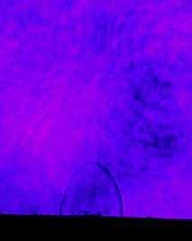
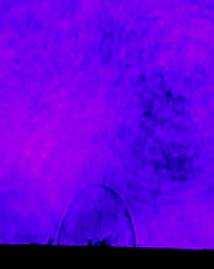
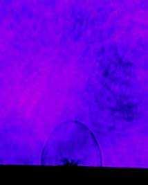
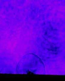
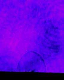
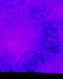
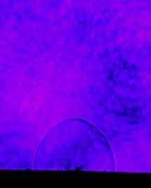
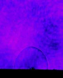
84 100 µm -2.4 ns 0.0 ns 2.0 ns 3.0 ns 4.0 ns 5.0 ns 6.0 ns 7.3 ns 7.9 ns 10.0 ns 13.0 ns 14.9 ns 19.0 ns 23.9 ns 25.8 ns 30.0 ns 33.1 ns 35.0 ns Figure 6. Shadowgrams for ablation with 1064 nm nanosecond pulse at 12.7 / 63

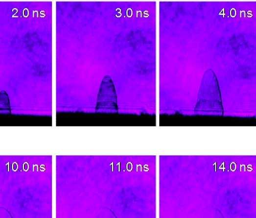
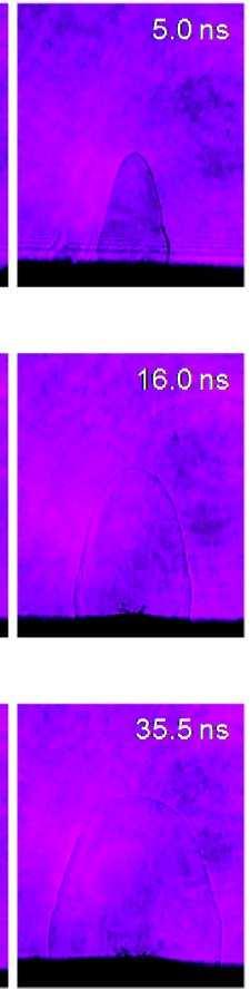
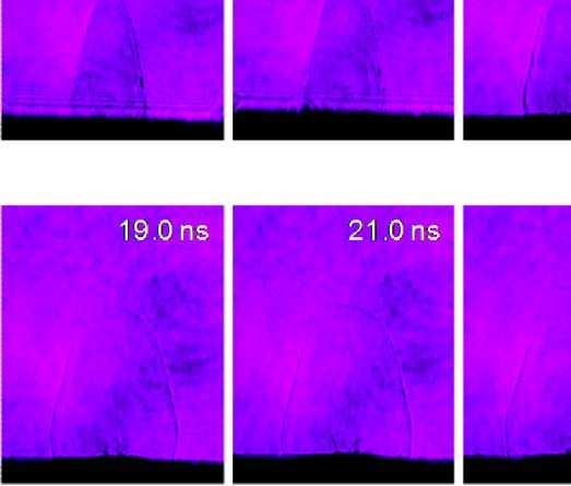
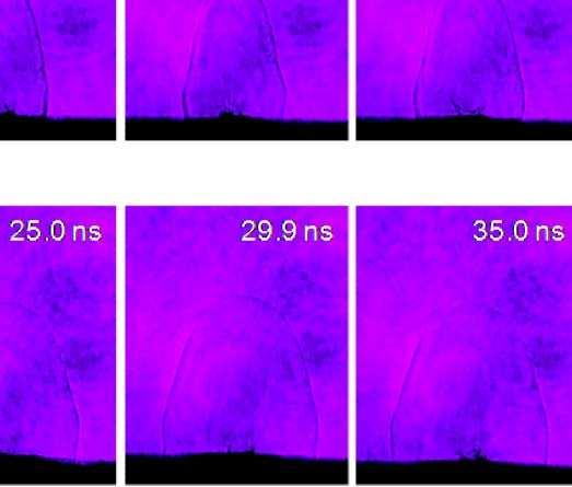
85 100 µm Figure 7. Shadowgrams for 1064 nm nanosecond ablation at 88.9 / 64

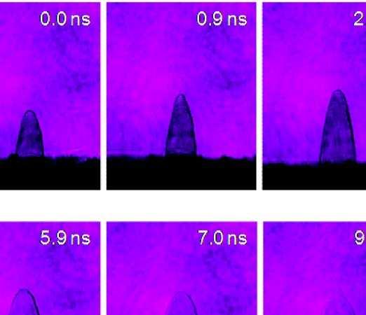
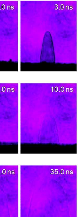
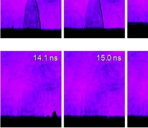
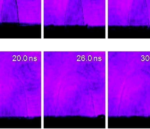
86 100 µm Figure 8. Shadowgrams for ablation with 1064 nm nanosecondpulse at / 65

87 As expected, the infrared regime presents a strong absorption of the laser pulse at its interface even at low fluence. This phenomenon is observed by the presence of two components in the expanding shockwave, which can be seen in Figure 9. The main component, spherical in shape, is best observed at short delays (represented by the dotted line). The second component, known as a laser-supported detonation wave (LSDW), is observed on top of the first one (represented by the plain line). This wave is the consequence of the absorption of the laser energy leading to a second breakdown process on the tip of the shockwave. The result is an elongated anisotropic shockwave expanding towards the axis of the incoming laser pulses. This anisotropy becomes more pronounced as the laser pulse energy increases due to greater plasma absorption of the laser pulse tail [1, 2]. The interface of the external shockwave has the highest electron density due to the compressing the surrounding gas by the ablated vapour. This particular point can reach values that are considerably higher than the average plasma density [2, 3]. This explains the observed laser supported detonation wave on the tip of the shockwave even at early delays. Figure 9. Laser Supported Detonation Wave of a plasma induced from a nylon sample in air for infrared nanosecond ablation. [1] The coupling between the incoming laser pulse and the sample is diminished as the plasma front absorbs the incoming laser pulse, preventing it from reaching the target surface. A part or all of its energy, depending on the extent of the absorption, is 66

88 transferred to the plume. Total shielding only occurs when the plasma has exceeded the critical electron density and starts to act like a mirror reflecting the laser pulse energy instead of absorbing it. This critical density has already been defined in Chapter I [12, 13] and reminded in Equation (1.2). We do not observe total plasma shielding as even at our highest fluences we do not attain such values. = 10 (2.1) With Chapter I also mentioned that for longer wavelengths, the main laser absorption mechanism is inverse Bremsstrahlung. For this mechanism, only one photon is absorbed. It means that it has a linear relationship with the laser intensity as opposed to a multi-photon ionisation that depends on the number of m photon absorbed ( ). We believe therefore that the laser pulse is absorbed by a greater surface area instead of being concentrated in the centre. Laser supported detonation wave Main shockwave Absorption surface Figure 10. Absorption of the income infrared laser beam by the plasma induced on a nylon sample. 67

89 Plasma axial extension (µm) Plasma transversal expansion (µm) mj 15 mj 10 mj 7 mj 5 mj 4 mj 3 mj 2 mj 1 mj Delay (ns) Delay (ns) Figure 11. Axial and transversal expansion of the plume. For a quantitative study of the expansion, the height and the width of the shockwave expressed in µm are presented in Figure 11. The radial expansion of the shockwave is the total width of the observed plasmas in figures 6, 7 and 8 divided by 2. The predominant axial expansion is obvious when comparing the two graphs. The axial expansion starts with a very high growth spurt and then levels out. The transversal expansion is more uniform with smaller expansion velocities. The difference in the two graphs put forth the ominant axial expansion associated with the anisotropic plasma. The curves for different energies follow the same tendencies except for the curve at 15 mj where a few abnormalities can be noted. The axial expansion graph starts off with an exponential growth followed by a linear expansion. The great expansion speeds observed at short delays (< 5 ns) correspond to the laser supported detonation wave effect on the plasma. From the data presented in figure 11, we can extract the axial expansion velocity as a function of the delay and for different laser energies by fitting the graphs with the equation below: ( )= 1 ( ) ( + ) (2.2) The parameters,,, are adjusted to fit the experimental data. The derivative of equation (2.2) was calculated and the expansion velocities are represented in figure 12 in function of the delay after laser pulse impact on the sample. It is important to state here 68

90 that this method remains preliminary and a more detailed model is necessary to understand the physics behind this phenomenon. Equation (2.2) simply allows us to have an idea of the expansion velocity. Plasma axial expansion speed (10 3 m/s) nm 20 mj 15 mj 10 mj 7 mj 5 mj 4 mj 3 mj 2 mj 1 mj Delay (ns) Figure 12. Calculated axial and transversal expansion speeds. Plasma transversal expansion speed (10 3 m/s) nm 20 mj 15 mj 10 mj 7 mj 5 mj 4 mj 3 mj 2 mj 1 mj Delay (ns) The axial velocity starts out extremely fast (between / ) and drastically slows down after 5 - uniform expansion can be observed. Considering the velocity is the derivative of the equation (2.2), the graphs will obviously tend towards (around 2 10 / except for 15 where c tends towards / ). We note that the velocities are much higher than the speed of sound (344 / in the atmosphere at 20 C), proving the agreement with the shockwave definition. The transverse velocity follows a different trend. Apart from the graph at 15 that tends towards a certain c value, the other curves do not follow this behaviour. The velocities continue to decrease even after 10 ns. [2] 69

91 ULTRAVIOLET REGIME Shadowgraph Images The following images were obtained with the shadowgraph procedure presented above. The wavelength of the ablation pulse was 266 nm provided by a quadrupled Nd:YAG nanosecond laser. We obtained images for various energies (1, 2, 3, 4, 5, 7, 10, and 15 mj) in the nanosecond ultraviolet regime, but again the following energies, 1, 7, 15 mj, are enough to depict the general plasma characteristics. They correspond to fluences of12.7 /,88.9 /, and / in figures 12, 13 and 14 respectively. 70

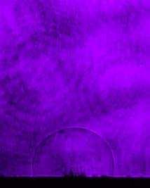
92 100 µm 0.4 ns 2.0 ns 4.0 ns 5.9 ns 8.0 ns 10.0 ns 12.0 ns 24.0 ns 28.0 ns 30.0 ns 34.0 ns 34.0 ns Figure 13. Shadowgrams for 266 nm nanosecond ablation at. / 71

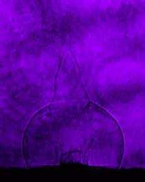
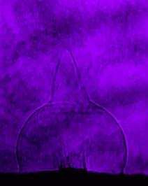
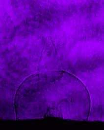
93 100 µm 0.0 ns 2.1 ns 4.1 ns 6.2 ns 8.0 ns 9.9 ns 12.0 ns 14.0 ns 18.0 ns 19.9 ns 22.0 ns 24.0 ns 28.0 ns 30.0 ns 34.0 ns 35.9 ns Figure 14. Shadowgrams for 266 nm nanosecond ablation at. /. 72

94 100 µm -2.1 ns -2 ns -1 ns 0.0 ns 1.0 ns 3.0 ns 4.0 ns 5.0 ns 6.0 ns 7.0 ns 9.0 ns 11.0 ns 14.0 ns 18.0 ns 23.0 ns 27.0 ns 33.0 ns Figure 15. Shadowgrams for 266 nm nanosecond ablation at. / 73

95 Our results show that the ultraviolet regime exhibit shockwaves that have a predominated semi-spherical form. However, for energies above 3, we observed small structures that grow on the tip of the shockwave, seen in figure 15. The appearance of these peaks is not regular from pulse-to-pulse, mainly due to the laser intensity variances that may occur and the difference in surface conditions at each ablation spot. This structure affects only part of the shockwave compared to figure 8 where the laser supported detonation wave protruded from a more global absorption. 1 mj 30 ns 3 mj 30 ns 7 mj 30 ns 15 mj 30 ns 100 µm Figure 16. Shadowgraph images for 1 mj, 3 mj, 7mJ and 15 mj at 30ns. The critical electron density is calculated at =1.4 10, which is 16 times greater than that for infrared ablation. Therefore, the electron density needs to be 16 times greater for shielding to occur, which cannot be obtained in our experiments. However, as the irradiance gets higher, the density of the interface increases and we can observe laser absorption. Ultraviolet ablation has a higher dissociation probability when compared to infrared ablation, due to its more powerful multi-photon absorption by air molecules (O 2 and N 2 ). The dissociation energies of the oxygen and nitrogen molecules are 5.2 and 9.8 respectively. O 2 dissociation needs to only absorb 2 photons while N 2 needs only 3 if we consider that a 266 photon has the energy of The irradiance required to form an air plasma is approximately / [5]. Due to the nonlinear 74

96 dependence of the photo dissociation rate with respect to the laser intensity, only the central part of the laser beam can induce a significant dissociation. This may explain the reason why the apparition of the second component is only located at the very tip and does not cover the whole upper part of the shockwave. The newly emitted free electrons continue to absorb the laser energy, which in turn, heat the incoming laser pathway. A laser ionised channel is therefore created locally, further facilitating the expansion at this particular point. The combination of both the non linear partial shielding and the laser ionised channel induces a sharp peak to emerge. Figure 17 shows the axial expansion of the main spherical shockwave with respect to the delay time. The different graph lines follow the same tendencies. Due to a higher slope below 10 ns, we can see that the plasma grew at a much faster rate at the beginning. We remark that in the ultraviolet regime, shockwaves expand spherically, which demonstrates the absence of a laser supported detonation wave in the ultraviolet ablation regime. We can also note that higher energies have a smoother fit. Plams axial extension (µm) nm 15 mj 10 mj 7 mj 4 mj 3 mj 2 mj 1 mj Delay (ns) Plasma transversal extension (µm) nm 15mJ 10mJ 7 mj 4 mj 3 mj 2 mj 1 mj Delay (ns) Figure 17. Axial and transversal expansion. 75

97 Again, equation (2.2) was used to fit the different curves in Figure 17. The derivative is calculated and plotted onto the graph below in Figure 18. Again, the graphs only give an estimate of the expansion velocities. The expansion speed starts out at a maximum and gently slows down to give us, in most cases, a constant value c, which varies more for these graphs than in the precedent Figure 10. The velocities reach a certain stability for energies 1, 2, 4 and 10 mj, while the others are still decreasing. Plams axial extension speed (10 3 m/s) nm 15 mj 10 mj 7 mj 4 mj 3 mj 2 mj 1 mj Delay (ns) Plasma transversal extension speed (10 3 m/s) Figure 18. Axial and transversal velocity expansion nm 15 mj 10 mj 7 mj 4 mj 3 mj 2 mj 1 mj Delay (ns) Fi 62T l l it i f ti fti As the energy increases, as shown in the shadowgraphs, other components can be observed at different times. Unlike the infrared regime, where only two components could be observed, the ultraviolet regime exhibits different components that become more complicated at high laser energies. This can be seen in Figure 19 where shadowgrams at 15 mj portray different components that appear at different time delays on the tip of the shockwave. Inside the plasma, we can see the presence of an interior shockwave and material fragment ejection [2, 3]. 76

98 Rapid emission Laser air plasma 2 nd bulb (LSDW) 3 rd bulb 2 nd bulb Main bulb Internal bulb Figure 19. Shadowgraph UV images at 10mJ. We can see the different components of the plasma clearly in these images. The thin peak that we see in the image (a) is due to the dissociation of N 2 caused by the passage of the laser. In figure (b) we see the laser supported detonation wave (LSDW) creating a second bulb. In (c) we see the apparition of a third bulb and in (d) the evolution of these three bulbs. Inside the main bulb, we see the presence of an interior bulb, which is due to the internal shockwave. The graph in Figure 19 below shows the specific expansion velocities of the components: the main spherical shockwave component with its two superimposed bulbs, and the two faster expanding components due to multiphoton absorption of the air molecules (green and blue). At higher energies, the ultraviolet shockwave expansion takes on different forms as the time delay varies. The earlier components (blue and green) are due to the laser passage in the air. The breakdown of N 2 and O 2 create a sensitive zone only locally. Due to which, the high interface density of the external shockwave explodes into the air where different components are interposed. 77

99 Plasma axial extension (µm) Figure 20. Axial extension of the different components of the choc wave. At very short delays, a very sharp peak was noticed but could no longer be observed after a few nanoseconds. This peak corresponds to the plasma induced in the air directly by laser pulse which can be clearly seen in figure 16a. An ultraviolet photon at 266 nm is equivalent to 4.67 and can dissociate oxygen molecules first. Another peak starts growing at the top of the main spherical shockwave (main bulb). As the plasma gets wider, so does this peak. However, there is a very erratic behaviour with its height. This may be due to the laser shot-to-shot energy fluctuation and the slight changes in the homogeneity of the target surface. At higher energies, there is even a third peak that appears. For larger delays (> 18 ) these three areas form a pear shape choc wave that gets larger as shown in Figure Delay (ns) 266 nm, 15 mj Component 1 Component 2 Component 3 Component 4 Component FEMTOSECOND ABLATION REGIME Figure 18, 19 and 20 show shadowgraphs of plasmas induced on the surface of a nylon sample by femtosecond laser pulses (800 nm) with pulse energies of 1, 3 and 4 mj. The observed shockwave expansions are essentially spherical putting forth the lack of interaction between the laser pulse and the induced plasma. However, the high intensity of a femtosecond laser pulse can induce an ionised channel in air before the pulse hits the sample, which is clearly observed in the shadowgrams for pulse energies at 3 and 4 mj. This ambient air conditions remain changed due to the filament even after the laser pulse is over, which creates a guided structure at the tip of the shockwave. 78

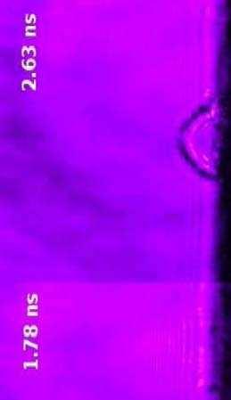
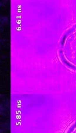
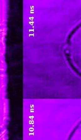
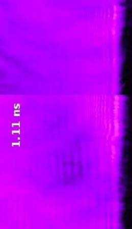
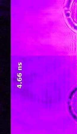
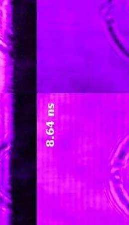
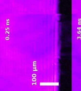
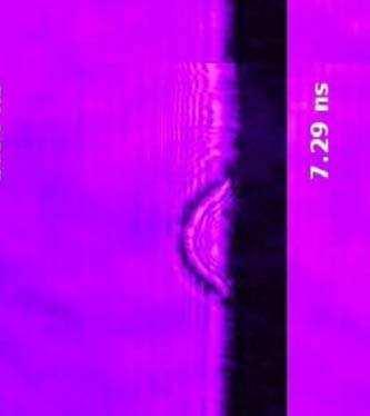
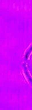
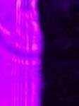
100 Figure 21. Shadowgrams for 800 nm femtosecond ablation at 1 mj 79

101 Figure 22. Shadowgrams for 800 nm femtosecond ablation at 3 mj 80

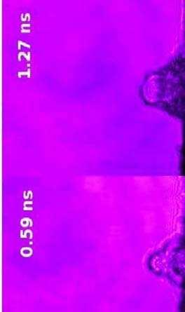
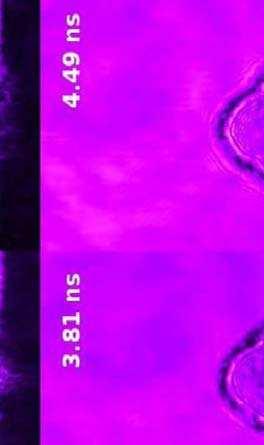
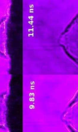
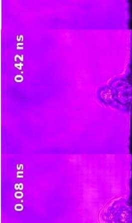
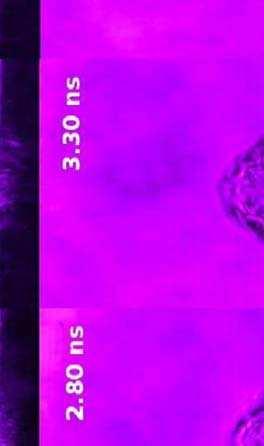
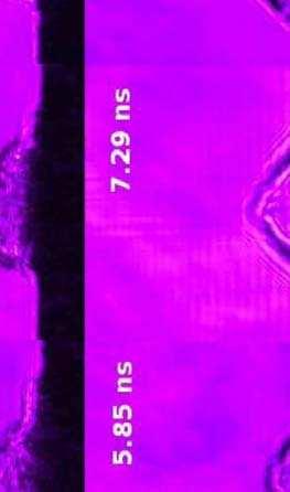
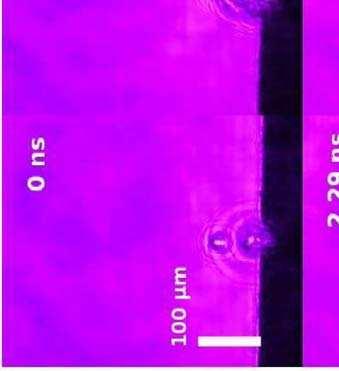
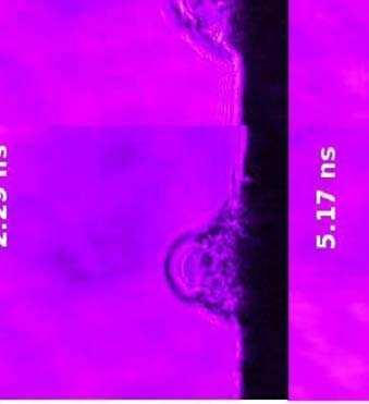
102 Figure 23. Shadowgrams for 800 nm femtosecond ablation at 4 mj 81

103 Figure 21 shows the axial expansion of the shockwave as a function of the delay. We can explain this observation by the fact that the femtosecond ablation regime allows a more effcient generation of nanoparticles creating a plasma with a lower degree of atomization [6]. Figure 24. Femtosecond linear axial expansion [7]. 3. DISCUSSIONS The primary melting and evaporation of the sample occurs during the first couple of nanoseconds. When the plasma plume is in contact with the incoming laser beam, its temperature and electron number density continue to increase. If the electron number density becomes higher than the critical number density, the laser pulse is blocked by the plasma front and can no longer attain the target surface. The entire laser energy interacts solely with the plasma in this case, subsequently heating it even more and causing its expansion speed to increase. The result is the formation of a second component called laser-supported detonation wave (LSDW), clearly observed in the infrared nanosecond shadowgraph images at higher energies. 82

104 In the nanosecond ultraviolet regime, the critical electron density required for shielding is much higher than in the infrared regime, making it more difficult to reach. The sharp peak could be the consequence of a local breakdown of the surrounding atmosphere due to the multi-photon ionisation caused by the high laser intensity. This dissociation becomes more evident in the femtosecond regime where the available higher laser intensity favours the air molecule dissociation followed by electronic detachment and ionisation. In the femtosecond regime, the laser pulse is already over by the time the plasma is formed and therefore cannot interact with it. Due to its ultrashort duration however, the intensity is significantly higher in this regime. The shadowgraph images (Figures 18 through 20) show the consequence on the ambient air of the passage of the laser pulse, which creates an ionised channel. The differences mechanisms involved in the three ablation regimes lead to for each regime, different shockwave morphologies. The infrared regime portrays an axial expansion which is significantly faster than the radial one due to a larger absorption and screening by the plasma of the incoming laser pulse. In the ultraviolet regime, the shockwave expands mainly in an isotropic way with partial screening leading to a second component that has a sharp peak. In the femtosecond regime, the expansion is spherical except for the very tip of the wave front that is influenced by this laser ionised channel. More detailed theoretical modelling is certainly necessary to understand the interplay of all these mechanisms which are responsible for the observed shockwave forms in the different ablation regimes. However, such modelling is out of the scope of the present thesis. We do know from the previous results that the shockwave front expands supersonically. To balance the velocity and the high backpressure generated by the external shockwave, an internal shockwave is produced, observed in our experiments only for the 266 nm ablation regime. The Berkeley team has a model that confirms the existence of the internal shockwave and how it moves back and forth between the sample surface and the external shockwave. They even show how some liquids are ejected as it strikes the sample surface due to the large amount of momentum transferred. They believe that the 83

105 interaction between the ejected liquid and the shockwave is the reason behind the rim around the crater after ablation. Our results also show a decrease in the shockwave expansion velocity as the ablation wavelength decreases. In the femtosecond shadowgraphs we remark a higher contrast compared to the nanosecond ablation regimes, which corresponds to a plume with higher density. For our choice in ablation regime, we eliminated nanosecond infrared ablation due to the strong screening presented. Despite that the plume had a higher temperature, we preferred to have the greatest amount of the laser energy used to ablate the surface of the sample and not heat the plume. Our choice was therefore between the nanosecond ultraviolet ablation and femtosecond regime. Before even starting our experiments we knew the delicateness and the cost of the femtosecond laser could be a problem for industrial applications. However, if we could prove that the results obtained by this regime were really more interesting than the ultraviolet ablation then it should be worth to use it. Since our aim is to find industrial applications from the results of this work, we opted for the nanosecond regime. The femtosecond regime remains very sensitive to the operation environment and demands more technical skills for its use. Nd:YAG nanosecond lasers cost less money and are less fragile, making them the more suitable choice for industrial application. In addition, published articles confirm that ultraviolet ablation is more efficient for organic samples. 84

106 4. CONCLUSION In this chapter, we have studied the early stage expansion of the plasma induced on the surface of a nylon sample in different laser ablation regimes with regards to pulse duration, wavelength and fluence. The aim was to select an optimised ablation regime for our LIBS analysis of organic materials in the atmospheric pressure. This regime can be provided by either nanosecond ultraviolet pulses or femtosecond pulses. Nanosecond infrared laser is less suitable for organic material analysis, because of smaller absorption coefficient of organic materials for infrared radiations. In addition, in this regime on top of the generated plasma, at high fluence, the absorption of laser energy by the plasma leads to shielding of the plasma. Such shielding decreases the energy coupled into the sample, reduces therefore the ablation efficiency. The correlation between the laser supported detonation wave and the high rate of recombination with ambient air for this regime was observed [1]. For nanosecond ultraviolet laser pulses at high fluence, energy deposited on the sample increases because the absence of pulse shielding by the plasma. The significant energy deposited on the sample increases the initial energy of the plasma which leads to a higher ionisation degree and a reduced molecule production. For application purposes, the use of a nanosecond ultraviolet laser with a much more compact and reliable system is obviously advantaged compared to a femtosecond laser who actually remains still more complicate to operate. 85

107 REFERENCES [1] M. Baudelet. Propriétés physico-chimique du plasma induit par laser en regime nanoseconde et femtoseconde. PhD Thesis Université Claude Bernard-Lyon 1, [2] C. Liu. A study of particle generation during laser ablation with applications. PhD Thesis University of Berkeley California [3] S.B. Wen. Experimental and theoretical study of laser ablation processes including vapor plume expansion, cooling, and condensation with an ambient gas. PhD Thesis University of Berkeley California [4] Longair, Malcolm S. Galaxy Formation. Berlin: Springer [5] J.H. Yoo. Enhanced Mass Removal due to Phase Explosion during High Irradiance Nanosecond Laser Ablation of Silicon. PhD Thesis University of Berkeley California [6] S. De Falco. Interaction laser femtoseconde métal : étude expérimentale des mécanismes d ablation et des formations des nanoparticules. PhD Thesis Université de la méditerranée- Aix-Marseille II, [7] M. Boueri, M. Baudelet, J. Yu, X. Mao, S.S. Mao, and R.E. Russo. Early stage expansion and time-resolved spectral emission of laser-induced plasma from polymer, Applied Surface Science, 255 (2009). [8] G.S. Settles. Sclieren and Shadowgraph Techniques, Visualizing Phenomena in Transparent Media [9] B. J. Garrison and R. Srinivasan, Laser ablation of organic polymers: microscopic models for photochemical and thermal processes. Journal of Applied Physics, 57, 2909 (1985). [10] X. Zeng, X. I. Mao, R. Greif, and R. Russo, Experimental investigation of ablation efficiency and plasma expansion during femtosecond and nanosecond laser ablation of silicon, Appl. Phys., A Mater. Sci. Process. 80(2), (2005). [11] [12] V.N. Rai, S.N. Thakur, Physics of Plasma in Laser-Induced Breakdown Spectroscopy. Laser Induced Breakdown Spectroscopy. Elsevier Science, Amsterdam, Netherlands, D.A. Cremers and L.J. Radziemski. Handbook of Laser-Induced BreakdownSpectroscopy

108 CHAPTER III. TIME-RESOLVED LIBS FOR CHARACTERISATION OF THE PLASMA INDUCED FROM POLYMERIC MATERIALS 1. INTRODUCTION The basis of LIBS is to detect and study the light emission from the induced plasma, which provides information of the analyzed sample. Previously, we made a choice regarding the wavelength that most suitable for polymeric samples and found that a nanosecond ablation wavelength at 266 nm was the most appropriate. The shadowgraph images also showed the supersonic expansion of the plasma, confirming that the characteristics of the plasma (temperature and electronic density) rapidly changes with regards to the delay after the laser impact on the target. This chapter shall focus on the choice of other experimental parameters, most importantly the delay after the laser pulse impact at which the spectrum acquisition should start ( ) 87

109 and for how long it should record the spectrum( ). For this, a presentation of our LIBS experimental setup will be given along with preliminary choices of our experimental procedure for spectra acquisition. Before going forth with any analysis, instrumental line broadening measurements were performed. This is followed by our spectrum acquisition procedure, explaining our choice for the different delays and gate widths for timeresolved LIBS. The number of spectrum chosen, along with the elements used for the plasma diagnostics are introduced as well. Once these criteria are chosen, time-resolved LIBS on polymeric materials can be properly investigated. We present our results regarding the electron density and different temperatures (mainly through Boltzmann plots and Saha-Boltzmann plots). The notion of local thermodynamic equilibrium is evoked for the use in calibration-free LIBS. For this thesis however, we are more interested in the signal-to-noise ratio that allows us to extract the most significant spectral information. Once these studies are finished, the optimal delay and gate width can be selected for the most reliable spectral line emission range (used in Chapter 4 for further LIBS applications). 2. EXPERIMENTAL SETUP In the following experiments, the fourth-harmonic generated (266 nm) by a Q-switched Nd:YAG laser (Thompson B. M. Industry 5000 series) was used at a repetition rate of 10 Hz. The laser pulse duration at FWHM was about 5 ns. The energy of this laser was varied between 1 and 20 mj. The harmonic generation was first optimised for generating 20 mj output at 266 nm. To obtain smaller energies, the phase-matching was detuned. The diameter of the laser beam was 7 mm. The laser beam was focalised onto the sample with the means of a fused silica lens. The focal length of the lens was 50 mm. An ablation crater with a 20 mj laser pulse on an aluminium sample is estimated to be 100 µm in diameter. Therefore, the estimated fluence was150 / ². The emission from the laserinduced plasma was collected by two aluminium-coated parabolic mirrors. The second one focalises the light emission directly into an optical fibre with a core diameter of 50 µm. A schematic representation is presented in Figure 1. 88

110 ns pulse laser (266 nm, 20 mj, 10 Hz) Figure 1. LIBS experimental setup. The emission spectra are analysed with the LIPSA software developed by our research group. To ensure the repeatability of the experiments, it is obvious that a rigorous experimental protocol has to be put in place. The first thing to do is to optimise the amount of light collected. Before any alignment is done, the distance between the focalising lens and the sample has to be fixed. We have chosen to place the sample right before the waist point of the laser beam to make sure that the ablation takes place inside the sample without direct air breakdown. The optical collection system is then aligned for this particular position. The parabolic mirrors are fixed to attain the smallest light spot. To finish the signal optimisation, the optical fibre entrance is positioned to attain the highest output signal. To clearly understand how this system works let us go back to the basics of light dispersion. The grating equation is stated in Equation (3.1). 89

111 sin ±sin = = (3.1) With : incident angle : diffracted angle k : diffraction order n : grating density : wavelength of diffraction R : resolution of diffraction (R = kn) An echelle spectrometer has the capability of separating both the diffraction orders k and the wavelength of the emission light received. This is why it is said to have a twodimensional wavelength dispersion. For high spectral resolution, a high dispersion element is needed such as echelle grating (Figure 2). When an incident ray is diffracted by grating, many spectra can occur. A low dispersion system like a prism is used to separate the overlapping of the light emitted by the echelle grating to produce high resolution and order separated spectra. This unique two-dimensional dispersion allows an atomic spectral line to produce an image in the form of a spot. Figure 2. Echelle Grating [1]. The Andor Mechelle spectrometer is a patented optical design that produces high resolution, broadband spectral ranges with low cross talk, based on the echelle grating 90

112 illustrated in Figure 3. The collected plasma light delivered by the optical fibre enters through the pinhole. The two correction lenses are used to decrease the loss of resolution that may occur. The collimating mirror reproduces an image of the source onto the prism. The downside to this is the overlapping of all the different spectral orders. The prism is used as a refractive element to separate these different orders. iccd camera Exit window Echelle grating Collimating mirror Flatfield lens Correcting lens Focusing mirror Entrance window Pinhole Double prism Dual Prism Single Prism Figure 3. Mechelle Andor Spectrometer and iccd [1]. To make the dimensional display even better, the use of two prisms results decreases the cross talk that can occur between the orders in the visible and NIR region, where the low dispersion forces them to bunch up. The resulting image is shown below in Figure 3, where a regular spacing between the spectral orders is seen with a dual prism. The advantage of such a system is the low cross-talk and equally spaced order separation for an optimal resolution with a wavelength ranging from UV to NIR. 91

113 The 2D map is focused onto the detector, which is an iccd camera (istar DH734 Gen II, Andor) in our case. The iccd camera has the advantage of offering high sensitivity in conditions with very low light available thanks to the intensifier. Its gating properties also provide very good temporal resolution for time -resolved plasma evolution studies. By receiving the two dimensional image, the camera can produce spectral images with high resolution. At the entrance of the CCD camera, there is an array of pixels. In our case we have pixels. The time it takes for the information to be gathered and sent out is a couple of microseconds. When the aim of our experiments is to look at what happens at very early and small time delays, the data readout time becomes a problem. To fix this problem, an intensifier is placed in front of the CCD. It acts as an electronic shutter that permits or prohibits light to enter. In other words, if the light beam lasts for one second, it will open the slit to CCD only for the desired amount of time, allowing only a fraction of the light to enter. It then closes, blocking the rest of the light. It can be done very fast and can be opened and closed within a matter of a few ns. This is the principle of gating shown in Figure 4. The intensifier presented in Figure 4 consists of a photocathode, a multichannel plate (MCP) and a phosphorus screen. The photons hit the photocathode, which due to the photoelectric effect, emits a certain amount of electrons. These negatively charged electrons with the help of a gate voltage are drawn to the MCP, which acts like an electron multiplier. The MCP has a lot of channels and when the electrons hit one of them, they get multiplied. The generated secondary electrons are accelerated towards the phosphorus screen due to the applied voltage. Once they hit the screen, their energy is transferred into the emission of a number of photons on the other side. The higher the voltage, the faster and stronger the electrons hit the screen, producing more photons. The photons are then projected onto the CCD camera. The advantage is that a lot more information is gained using this technique but because it has more optical components, we lose some resolution. 92

114 Applied Voltage Input Window Fiber Optic Output Window Photocathode Photons Microchannel Plate (MCP) Phosphorus Plate Applied Voltage Figure 4. The intensifier [1]. 3. PRE-SPECTRA ACQUISITION Before starting our time-resolved experiments, a few necessary details need to be adjusted. Notion of instrumental broadening will allow us to affine our calculations regarding the temperatures and electronic density of the plasma. Preliminary spectra were recorded to provide us with information regarding the delay and gate width to choose at different moments. Finally, the choice of how many spectra is sufficiently enough for our time-resolved analysis INSTRUMENTAL BROADENING As explained in Chapter 1, an instrumental broadening must be accounted for spectral analysis. Our best line fit for such broadening is the Gaussian fit with R² = 0.99 as compared to the Lorentzian fit with R² = 0.96 as can be seen in the Figure 5 representing a spectral line emitted by a mercury lamp. 93

115 Wavelength (nm) Figure 5. Simulation of a mercury lamp emission fitted with a Gaussian and a Lorentzian graph Normalised intensity (a.u.) The instrumental broadening may depend on the wavelength. Different wavelengths from a low-pressure mercury lamp were used to measure this broadening as a function of the wavelength. Figure 6 puts forth our results and the instrumental resolution power determined experimentally was ½ =9010 ±150 (the constructor had announced ). There is less fluctuation at shorter wavelengths (~0.03 nm) than at longer wavelengths (~0.07 nm). Instrumental width at half maximum (nm) ( / 1/2 ) = R² = ( 1/2 ) = 1.11 x 10-4 Wavelength (nm) Figure 6. Instrumental broadband broadening. 94

116 3.2. DELAY AND GATE WIDTH Our first aim was to study the time-resolved spectral emission of the plasma by calculating different temperatures and electronic densities as functions of the delay after the laser impact. For this study, we fixed the following experimental parameters accordingly. The camera exposure was always fixed at 1s, which means that each spectrum is the accumulation of 10 laser pulses since the laser is working at 10 Hz. A reason behind this choice was to accumulate the spectra to increase the signal intensity and reduce some of the noise. The delay is the moment after laser impact upon the sample where the acquisition starts and the width corresponds to the duration that the camera is gated (Figure 7).. Impact after laser pulse (delay) Gate Width (spectra acquisition) Laser pulse t d t b ns Figure 7. Chronogram of spectra acquisition. Longer delays allow the plasma to reach equilibrium but also give less intense signals. At earlier delays, there is a rapid change in the electronic density and temperatures due to the extremely fast expansion of the plasma as explained in Chapter 1. For earlier delays, in order to avoid large differences between the spectral data acquired at the beginning and at the end of the acquisition, smaller gate widths should be chosen. At longer delays, the fluctuations dampen out i.e. these effects are less consequential, allowing us to choose larger gate widths to acquire more signal. In other words, we have segmented the plasma acquisition times into different categories as can be seen in Table 1. We assume that between 70 ns and 130 ns (gate width of 30 ns), the plasma is almost stationary. The same reasoning goes for 1980 ns and 3980 ns. 95

117 Delay (ns) Gate width (ns) Table 1. Spectrum acquisition parameters. 4. EXPERIMENTAL RESULTS 4.1. STATISTIC SPECTRAL ACCUMULATION The question on how many spectra should a statistical series contain was evoked. When gathering information for a statistical spectra batch, we kept all the parameters fixed while we scanned the surface of our sample. Every spectrum was issued from a plasma that was induced on a fresh surface and not the accumulation at the same ablation spot. For example, for a fixed delay of 380 ns and gate of 100 ns, all the spectra were acquired under the same conditions except for the experimental fluctuations and the local sample inhomogeneities. We did a quick study comparing the results regarding the temperature and electronic density of the statistical batch containing information from 10 and 100 spectra. 96

118 100 ACCUMULATIONS 10 ACCUMULATIONS Delay (ns) Gate width (ns) Delay (ns) Gate width (ns) Table 2. Spectra acquisition parameters for quick measurements Figure 8 shows the estimations for both the electronic density (with regards to the line) and the temperature calculations with regards to calcium elements [4, 5]. With a 100 spectra statistical batch, we are able to scan a relatively large surface area of the sample. Since a perfectly homogenous sample is only really theoretically possible, this scanning can dampen out any local differences on the sample s surface. The experimental conditions are also prone to slight fluctuations (energy of the laser, the position of the sample with respect to the beam focusing point, inhomogeneity of the sample etc.) Figure 8 shows that the accumulation of a 100 spectra provided more accurate results, especially when calculating the electronic density. The dispersion of the points was far too great with regards to the statistical batch containing 10 spectra to provide us with measurements that are good enough. Figure 8 also shows dots that are present for one statistical series and not the other. The time required for the 100 spectra acquisitions are 10 times more time costly. Therefore, the graphs were composed of the data corresponding to the parameters in Table 2. 97

119 14000 Electronic Density (cm -3 ) 1E18 1E17 R² (10 accu) = R² (100 accu) = Temperature (K) R² (10 accu) = R² (100 accu) = accumulations 10 accumulations Delay (ns) Delay (ns) Figure 8. Comparison between the accumulation of 10 and 100 spectra taken on a polypropylene sample ablated in air TEMPERATURE COMPARISON The atomic temperature can be calculated with regards to 3 elements in our case: magnesium (Mg), titanium (Ti), and calcium (Ca). Their temperatures are presented in Figure 9 showing the different values produced by Saha-Boltzmann plots previously explained in Chapter 1. Magnesium exhibits the highest temperature values and calcium the lowest ones. Titanium contains much more spectral lines compared to the other tow elements that only have 3 line for each (either ionic and neutral lines). For the rest of our temperatures calculations, it seemed that the titanium results provided a more accurate estimation and shall be used Temperature (K) Ti Ca Mg Delay Figure 9. Temperature calculations on a polypropylene sample. 98

120 Figure 10 puts forth the average of a 100 spectra for a polymer sample at different laser pulse impact delays. For shorter delays, the total emission spectrum experiences a large influence of the continuum emission since the baseline of the spectrum is high. As the delay increases, the radiative recombination between electrons and ions and Bremsstrahlung emission drop, decreasing their influences. After about 500 ns, our spectrum is dominated by spectral line emissions associated to optical transitions between discrete states of different species, ions, atoms and molecules. As the delay increases, the electronic density decreases resulting in spectrum narrowing. Figure 10. Evolution of the spectrum for a polymer sample. Carbon and hydrogen are the elements most commonly present in all polymers. Oxygen and nitrogen can sometimes be present as well. However, if the ablation process is done in the presence of air, hydrogen, oxygen and nitrogen can also be due to the contributions from the ambient air. Certain additives and fillers are added to polymers to improve their properties or simply to reduce the cost of fabrication. The most commonly found are 99

121 TiO 2, CaCO 3, and Mg, with variable concentrations [2]. This is explained in more detail in the next chapter. In our experiments, we use these elements to calculate electron density and different temperatures. To find the best compromise between maximal intensity and maximal signal, we also studied the signal-to-noise ratio (SNR). It will be shown that this compromise coincides with the conditions for the local thermodynamic equilibrium as well ELECTRON DENSITY Time-resolved LIBS was used to characterise the plasma induced on a polypropylene sample. Temporal evolution of the electron density was determined for the ablation energies of 18 mj. The Stark broadening of the line was used to calculate the electron density [6]. As shown in Figure 11, it starts out higher at about 1 10 at short delays then decreases to about 1 10 for longer delays. The self-absorption of the line only starts to appear for electron densities greater than3 10 [3]. Therefore, despite hydrogen being part of the matrix, we can ignore the self-absorption of the in our calculations. After 1500 ns the line became undistinguishable amongst the noise, rendering the evaluation of the electronic density impossible. 1E18 PP Sample 15 mj Electronic Density 1E Delay (ns) Figure 11. Electron density for polypropylene sample at 18 mj. 100

122 As mentioned in Chapter 1, the McWhirter criterion provides the lowest value for the electron density necessary (but not sufficient) for the plasma to reach local thermodynamic equilibrium. For a 7000 K plasma, it can be estimated at = In Figure 11, the measured electron densities are larger than this value. This means that the plasma has enough electrons to reach local thermodynamic equilibrium through collisions TEMPERATURE CALCULATIONS Given these electron density, the following temperature calculations were done using plasmas induced by 18 mj laser pulses upon a polypropylene sample. For the evaluation of the line intensities, a question on whether it was better to use the total surface area under the spectral line or just the peak maximum value was asked. Figure 12 shows the results from the both methods taken simultaneously. We can see that for delays less than 300 ns there is a difference between the two methods. However after this delay, both provide comparable results. Therefore to simplify the calculations, we use the peak maximum since it is less time consuming. Surface area under the spectral line Maximal peak of the spectral line Mg Ti Ca Molecular temperature Figure 12. Temperature calculations comparing the spectral peak maximum (open dots) or total surface (asterisk) and the molecular CN temperature (stars) 101

123 Boltzmann plot The aim is to plot information taken from different spectral lines of the same species (neutral or ionic) and draw the best fitting line. According to the Boltzmann distribution law, the slope of this line is related to the temperature of that particular species. As can be seen by Equation (3.2), the intensity of a spectral line is inversely proportional to the temperature [6]. (3.2) The temperature of the plasma can be found by calculating the slop of the line, as shown in Figure 13. The atomic neutrals are on the upper left side of the graph while the ions are in the bottom right side. It can be seen that it is not a very accurate means due to the large vertical dispersion of the points and a narrow energy scale concerned, especially for the atomic neutrals. We will see later that the Saha-Boltzmann plot provides more accurate results in for temperature calculation. ln ((Iij ij ) / (g i A ij )) Ti I R² = Ti II R² = Ti (II) Ti I + Ti II Ti (I) R² = E i (ev) Figure 13. Boltzmann plot for titanium species at a delay of 1370 ns and gate width of 800 ns 102

124 Saha-Boltzmann Plot If we assume that the ions and the neutral atoms of the same element are said to be at the same temperature, we lift the problem encountered with the Boltzmann plot. We can now trace a line that goes through both species simultaneously. The errors associated to linear fits are now improved as the horizontal energy range has increased considerably compare to previous Boltzmann Plot. We recall the Saha-Boltzmann ordinate correction in Equation (3.3). The approach remains very similar to the Boltzmann plot where the aim is to find the best fitting line and calculate its slope to find the plasma temperature [4]. Typical Saha-Boltzmann plots are shown in Figure 14 for different delays starting off from 170 until 1370 ns to show the temporal evolution of the temperature. These plots exhibit a good linearity with statistical errors associated to the retrieved temperature at less than 100 K. Good agreements are especially observed between the atomic (left side) and ionic (right side) transitions. This agreement indicates that equilibrium is reached between neutral and ionised titanium atoms [6]. = 2 (2 ) / / (3.3) The wider energy range allows for more precise linear plots by combining both species of the same element. Different delays are presented on the same figure to put forth the difference in their slopes. A greater slope indicates a lower temperature. 103

125 Figure 14. Saha-Boltzmann plots with lines from Ti LOCAL THERMODYNAMIC EQUILIBRIUM Considering the McWhirter criterion, the electron density must be high enough for the local thermodynamic equilibrium to be considered [4]. In Chapter I we calculated this density for a plasma at 7000 K using the line is = The calculations show that the electron density ensures this density until a delay lower than 1 µs. The second criterion for local thermodynamic equilibrium states that the plasma needs to be defined by a single temperature to describe the different species present. This means that the neutral and ionic species of all the elements must be at the same temperature along with the molecular temperature. For this, we perform a study of the evolution of the temperatures in the plasma to verify this condition. The different plots are represented in Figure 15. In this figure, the excitation temperature of Ti ions is calculated for different delays using the Saha-Boltzmann plot. According to 104

126 Equation (3.3) the electron density is needed. The electronic density data shown in Figure 15, which corresponds to 18 mj ablation laser energy, is fed into Equation (3.3). Calculations are only available until a delay of 1 µs due to the disappearance of the line. The electron densities beyond this point are obtained by extrapolating the experimental data using a power law fitting. The different temperatures merge together after 600 ns, with a maximal value for the molecular temperature between 700 and 800 ns. The density criterion is satisfied only until about 1000 ns. In order to consider ourselves in local thermodynamic equilibrium, it would be better to place ourselves with a delay of 600 ns. The gate width of 400 ns was chosen in order to get the maximal amount of intensity out of the spectral information. The fluctuations between the temperatures are still seen to fluctuate for this time frame, however it was the best compromise to satisfy the local thermodynamic conditions. Temperature (K) Electronic density criterion satisfied, p Vibrational CN Smooth CN SHB Ti Ionic Mg BP Ti I Delay (ns) Figure 15. Temperature temporal evolution. 105

127 4.6. SIGNAL TO NOISE RATIO To estimate the signal-to-noise ration, the background intensity is subtracted from the maximal peak intensity of of a given spectral line. The result was then divided by the noise, calculated by the standard deviation of the background emission close to the considered line. The signal to noise ratio is thus given by Equation (3.4) [4]: = (3.4). Figure 16 shows the temporal evolutions of the SNR of some elements detected in a polymer sample. We can see that the maximum values of SNR are achieved between 300 and 1000 ns if we take the carbon line and the CN line maximums for our limits. The local thermodynamic equilibrium range found before was satisfied between 600 and 1000 ns. The best compromise between these two values regarding our measurements, would be to take start the acquisition after a delay of 600 ns after laser impact for a duration of 400 ns. Signal - to - Noise Ratio Delay (ns) Figure 16. Signal-to-noise ratio for a polypropylene sample at 18 mj CN (387) Ti I (430) Ti II (335) Mg II (280) C 247 Ca II (393) 106

128 5. CONCLUSION Through time-resolved LIBS we observed the evolution of the electron density of the plasma. This allowed us to measure the different temperatures of the plasma using Boltzmann or in a more advantage way, Saha-Boltzmann plots that provided us with more accurate temperatures due to the larger energy range by using emission from both ions and neutral atoms. We were also able to estimate the molecular temperature for CN and C 2 molecules. The convergence of the different types of temperatures and the sufficient electron density ensure the condition for the local thermodynamic equilibrium. For the following works concerning the coupling of LIBS with artificial neural networks (ANN), local thermodynamic equilibrium conditions are not what are important for us. For LIBS to find its place in the industry it needs to be efficient i.e. provide accurate results in a minimal interval of time. For this, it needs to identify polymer samples using their essential and optimal information, which means at the best signal-to-noise ratio. The fact that this temporal range coincided with the local thermodynamic equilibrium range is reassuring as local thermodynamic equilibrium provides the best conditions for the extraction of spectral information. Therefore, our time-resolved LIBS analysis presented in this chapter has led us into choosing our ideal experimental configurations for the next step. The LIBS spectrum will be recorded 600 ns after the laser pulse impact upon the sample during 400 ns. ( =600 =400 ). 107

129 [1] Andor Technology Website, [2] C.E. Wilkes, J.W. Summers, C.A. Daniels, M.T. Berard. PVC Handbook. Hanser Gardner Publication Inc [3] J. Ashkenazy, R. Kipper, M. Caner, Spectroscopic measurements of electron density of capillary plasma based on Stark broadening of hydrogen lines, Phys. Rev., A 43 (1991) [4] W. Lei, V. Motto-Ros, M. Boueri, Q. Ma, D. Zhang, L. Zheng, H. Zeng, J. Yu. Time-resolved characterization of laser-induced plasma from fresh potatoes. Spectrochimica Acta Part B 64 (2009) [5] O. Barthélemy, J. Margot, M. Chaker, M. Sabsabi, F. Vidal, T. W. Johnston, S. Laville, and B. Le Drogoff. Influence of the laser parameters on the space and time characteristics of an aluminum laser-induced plasma. Spectrochimica Acta Part B, 60 : ,

130 CHAPTER IV. DISCRIMINATION AND IDENTIFICATION OF POLYMERS USING LASER- INDUCED BREAKDOWN SPECTROSCOPY 1. INTRODUCTION 1.1 POLYMERS Polymeric materials are used in our everyday life in many forms, from disposable containers for household products to construction materials used industrially. The main building blocks, except for a few exceptions, are carbon and hydrogen, but other elements such as oxygen and nitrogen are very commonly found as well. These main elements form monomers, which are essentially organic based (C, H, O and N). The specific ways in which these chains are aligned and twisted together define the material s physical properties. If the alignment of the monomers is random it gives rise to amorphous plastics, which are known for their impact strength and toughness. Examples include polyvinylchloride (PVC), polycarbonate (PC), and polystyrene (PS). If the monomers are 109

131 orderly and densely packed it leads to crystalline polymers, which are less flexible and have lower elongation properties than amorphous ones. Polyamide (PA), polyethylene (PE), and polypropylene are some examples. However, even though the physical properties are important for their diverse uses, it is also essential to understand what kind of bonds make up the plastic to help understand how to recycle them Thermoplastics and Thermoset Plastics Apart from how the monomers can be arranged, the nature of the polymer bonds also has an impact on its physical properties. Depending on the nature of these bonds, polymers can be either thermoplastics or thermoset. The bonds are weaker for thermoset plastics giving them the property of being heat sensitive, i.e. they can be melted given the right temperature. This property is extremely useful as it facilitates the recycling purposes. Thermoplastics suffer only chemical degradation when a significant amount of heat is applied due to their stronger bonds. These plastics require more complicated recycling processes that are not yet very attractive to the recycling industries. Even though technically all plastics have the potential to be recycled, for the time being, the focus is on thermoset plastics (especially polypropylene (PP) and polyethylene (PET)). The ones that cannot be recycled are dispatched into landfills or sometimes burned [1] Plastic Consumption and Production One can logically assume that if the production of plastics increases the amount of plastic waste increases accordingly. Figure 1 shows the increase in European and world plastic production between 1950 and Figure 2 shows the evolution of how landfilled and recycled plastics between 1995 and Even though recycling tendencies have risen, the efforts remain less significant compared to the total waste increase. Improving the recycling process might be one way of reducing this huge difference between the plastic production and waste recycling. 110

132 Million tonnes Year Figure 1. Increasing European and world plastic production. Includes thermoplastics, polyurethanes, thermosets, elastomers, adhesives, coatings, sealants, and polypropylene-fibers but not polyethylene-, polyamide- and polyacryl-fibers [2]. For the time being, virgin plastics remain relatively cheap to produce compared to recycled plastics. Recycled plastics are becoming more attractive from an ecological and soon a financial point of view. Plastics have an extremely long lifetime adding to the landfill overpopulation problem. Burning them leads to the possibility of transmitting potentially dangerous and harmful elements in the atmosphere. The production of plastics consumes a lot of petrol, where it is said that 4% of worldwide petrol consumption is used for the production of plastics and another 3-4% is used in their manufacture. Petrol, being natural resource, is running out and will cause the prices to increase drastically over time. This tendency is already beginning to show in the past years already, as shown in Figure 2. As petrol prices keep increasing, so will the price of virgin plastics (a). Weekly Gasoline prices in the USA that show an exponential increase since 2002 (b).therefore, the 1.8 tonnes of oil saved per tonne of PET bottles recycled might not be worth much now, but with future sky rocketing oil prices, the save will become more valuable. Other solutions other than recycling may exist, nonetheless, it has a positive and non-negligible participation to the global efforts for an ecological solution for the future. Figure 2c shows the increase in recycling of PET bottles between but also the increase in the amount that are landfilled. [3] 111

133 a) b) (Log scale) c) Figure 2. a) Total world oil production [4]. b) Oil prices since 2002 [5]. c) Evolution of PET bottles [4]. 112

134 1.2 RESIN IDENTIFICATION CODE Therefore, industrial and domestic waste recycling offers an essential contribution towards environmental protection through sustainable development all the while providing economical benefits. The first step of recycling starts with sorting, whether it is at a domestic level or an industrial level. The American Society of the Plastic Industry (SPI) introduced a resin identification code system in 1988 to identify the main polymers encountered in the residential waste stream [6, 7]. Their aim was to help people sort their domestic waste to initiate recycling in homes. The code brings together the six main polymers that are mostly used in the household. Each number is associated to the type of material used and are listed in the Table 1. Code System Associated Plastic Examples PETE (polyethylene terephthalate) HDPE (high density polyethylene) PVC (polyvinyl chloride) LDPE (low density polyethylene) PP (polypropylene) PS (polystyrene) Other (the rest of all plastics) Water and soft drink bottles Household bottles (cosmetics, food, detergent), industrial wrapping Medical bottles, water pipes, window panes, credit cards, flooring Garbage bags, food wrap Yoghurt containers, margarine containers, milk and beer crates Disposable cups and plates, egg cartons Plastic mixtures Table 1. Resin identification coding system implemented by the Society of Plastic Industry (SPI) Due to blending incompatibilities, different plastics cannot be mixed together when recycled. When different types of plastics are melted together they tend to phase-separate, like oil and water, and produce layers. The phase boundaries cause structural weaknesses in the resulting material, meaning there exists only limited useful applications for polymer blends. A main concern is the emission of toxic gasses due to certain combinations such as PVC and PET. Therefore, to avoid dangerous outcomes to both the employees and the environment, they must be identified and sorted beforehand. Another barrier to recycling is the widespread use of dyes, fillers, and other additives in plastics. If the separation of fillers is not carefully optimised the plastic can be damaged in the process. Additives are less widely used in beverage containers, allowing them to be recycled more frequently [8]. 113

135 1.3 SORTING TECHNIQUES Even though sorting can start in the household, large scale and more refined methods are required at an industrial scale. This leaves sorting industries with a choice between two methods: manual or automated sorting Manuel sorting Manual sorting consists of employees manually looking for the Society of Plastic Industry resin code identification on arriving plastic on waste stream belt as shown in Figure 3. (a) Employees first sort out the whole waste stream taking out things that should not be present. (b) Once plastics have been separated from the basic waste stream, a team does extra sorting to separate the different kinds of plastics. Once the code is found, the plastic is disposed in the specific batch with other like materials. This method has not proved to be very efficient for many reasons. Firstly it is time consuming as the resin coding system is not always easy to identify, especially with crushed and damaged containers. Secondly, employees are in direct contact with the waste stream, where appropriate protection is needed due to the heavy bacteria filled environment. This task is physically enduring due to the long hours and repetitive movements. There are also possible toxic gas releases if PVC is wrongly mixed with PET bottles [9, 10, 11]. The non-negligible human errors are urging industries to find automated and cost-effective methods to perform reliable sorting of plastic wastes. a) b) Figure 3. a) Pre-manual sorting to remove big contaminants. b) Manual plastic sorting. 114

136 1.3.2 Automated Systems Automated systems that provide fast identification are the best answer to these industrial demands [12]. Pre-sorting solutions can be found within the optical sorter technologies. Their ability to detect plastic materials from paper, metals and glass rapidly is very useful [13]. They are most commonly used in the food sector to separate plastic bottles from other materials and may also provide colour detection. The second step, which is polymer sorting, is done with more sophisticated spectroscopic methods. There are a few techniques that stand out for the moment [14]. a. Near infrared (NIR) spectroscopy One of the most commercially available technologies, operating in a spectral range of nm [15-18]. It identifies the molecular structure of polymers by detecting their reflection or transmission spectrum. The identification is done quickly with a response time sometimes in the order of 100 ms. Despite its accuracy and rapidity, it cannot analyse black or very dark samples. Most of the radiation gets absorbed leaving hardly anything reflected back to allow the analysis to take place i.e. featureless spectra [19, 20]. This represents a problem, for example for the automobile industry where black or dark plastics are largely used. This technique also needs to be in contact with the sample to identify it. b. X-ray fluorescence spectroscopy Mainly used in the industry for its ability to detect a single element: the chlorine atom. When a plastic stream is predominantly filled with PET bottles it can quickly detect the PVC bottles that can be scattered by making them stand out [19]. There are two kinds of X-ray detectors in the industry [7,20] : XRF (x-ray fluorescence): the x-rays are detected once they bounce off the surface of the bottles. PVC bottles that are shielded by other PET bottles are not detected with this method. XRT (x-ray transmission): the detection is done once the x-rays pass through the bottles. More efficient due to its ability to detect PVC bottles even if they are hidden behind other PET bottles. 115

137 The disadvantages of this technique are its ability to only separate PVC bottles from the plastic stream and the security risks associated with x-rays. X-rays are a form of radiation and special precautions are required to protect employee exposure. X-ray detection systems need to be cleared and registered by the Nuclear Regulatory Commission (NRC). c. Raman spectrometry A spectroscopic method that uses monochromatic laser light (mostly visible or NIR) that is scattered once it is reflected upon the Raman sensitive samples such as a plastic surface. The re-radiated scattering of light causes differences with the original monochromatic light that puts forth the different molecular structures of each polymer [21, 22]. The detection time remains relatively too long to use for industrial uses. d. Laser-induced breakdown spectroscopy (LIBS) As already recalled throughout this thesis, LIBS has strong potential that should meet the requirements of the industry. It is not limited by the colour of the plastic like NIR spectroscopy, i.e. dark and black samples. It can also take things a step further by detecting metallic trace elements, fillers, reinforcements and additives [12]. With its intrinsic advantages, LIBS can become an attractive technique, particularly when combined with other existing ones for online and real-time identification of plastics [1, 23]. In this chapter we will especially demonstrate that a large LIBS spectral range combined with the artificial neural networks (ANN) [13, 15] provide reliable and fast identification of different types of plastics. 2. SAMPLE PRESENTATION AND SPECTRAL RESULTS The same experimental setup as demonstrated previously in Chapter 3 was used here. It was found that a delay of 600 ns and a detection gate width of 400 ns provided the highest signal-to-noise ratio (SNR). In this detection window, the plasma can also be considered homogeneous and in local thermodynamic equilibrium (LTE). Statistical series were then performed with these detection parameters on the polymer samples. This means that for 116

138 each sample, two sets of 100 spectra were recorded in the same conditions with the same experimental parameters at an integration time of 1 second per spectrum. To account for the possible environmental and experimental changes that can exist in the industry and affect a LIBS setup, the first set was taken a few weeks before the second one. This was the only difference between the two. In order to compare our experimental conditions to those used during routine analyses, each spectrum was recorded with the short integration time of 1 second, which corresponds to the accumulation of 10 laser shots. Samples were cleaned with methanol before measurements. Finally, the data analysis was done with the help of the LIPSA software developed in our research team. 2.1 SAMPLE PRESENTATION LIBS measurements were first done on the eight following reference samples (Figure 4), which cover different varieties of polymers used domestically and industrially. A combination of dark, white and transparent samples is used in our studies. The common element being carbon and hydrogen (except for PTFE which has fluorine instead of hydrogen).this set contains polymers within the resin identification code (PP, PVC, PE500) along with a thermoset plastic (PTFE), a polyamide (PA 6,6), and other plastics commonly used in the industry. They are homogeneous sheets of plastic and their colour ranged from transparent to dark and opaque. Prior to our experiments all the samples were initially smooth and cleaned with methanol. DARK SAMPLES WHITE SAMPLES TRANSPARENT SAMPLES PVC Polyvinylchloride PA 6,6 (Nylon) Polyamide 6,6 PE (Polipolen) Polyethylene 500 gr/mol PMMA (plexiglas) Polymethylmethacrylate PP(Prolene) Polypropylene mesh POM (Delrin) Polyoxymethylene PTFE (Teflon) Polytetrafluoroethylene PC Polycarbonate Figure 4. Polymer reference samples 117

139 2.2 EXPERIMENTAL SPECTRA Typical LIBS spectra are presented for PVC, PTFE, PP and PC in Figure 5. A broad spectral range between 240 nm and 820 nm permits the detection of spectral lines used to identify different atomic elements and molecular bands. Carbon and calcium are saturated in the graphs in order to accentuate the intensity of weaker spectral lines. The molecular elements, such as CN and C 2 bands, are more likely to be seen in the ultraviolet region. Most of organic elements, such as hydrogen, nitrogen, and oxygen, can be observed in the near infrared range. We can also notice the presence of trace elements such as Ti, Mg and Ca, visible in the ultraviolet range for PP and PVC, while none were observed for PTFE and PC. These metallic traces are often used to reduce production costs and/or to improve physical and mechanical properties [24]. The atomic elements, such as chlorine and fluorine, are observed in the visible and infrared regions. The absence of hydrogen in PTFE can also be noticed. PC and PMMA, which are both transparent samples, did not contain any trace elements or charges. This absence can also be noted for the white PTFE sample. 118

140 (a) C Mg Ca Ti 1x10 6 PVC C 2 CN Ca 0 Intensity (counts) 4x10 5 2x x10 5 6x10 5 3x PTFE PP (b) Intensity (Counts) 3x10 5 2x10 5 1x x10 5 5x x10 4 4x10 4 2x x10 5 5x x10 5 5x10 4 PC Ca Ti PVC PTFE PP PC C 2 C 2 Na (c) 3x10 5 2x10 5 1x Fl H Fl Cl N O PVC Intensity (Counts) 3x10 5 2x10 5 1x x10 5 1x x10 5 2x10 5 PTFE PP PC Wavelength (nm) Figure 5. Spectra of PVC, PTFE, PPM and and PC PC in in the the a) a) Ultraviolet, b) b) Visible and and c) c) Visible and and near infrared ranges. 119

141 3. SPECTRA ANALYSIS 3.1 STOICHIOMETRIC RATIO At first, we were curious to see the difference between the C/H experimental and theoretical ratios. The stoichiometric ratios from the molecular formula of the matrices were calculated for each sample as shown in Table 2. The theoretical variations of C/H go from 1/2 to 2/3 with the exception of PTFE, which contains no hydrogen. The experimental ratios measured using the spectral line at 656 nm and the C line located at 247 nm were calculated and compared with the theoretical ratios in Table 2 and displayed in Figure 6. Other elements present in the matrix could be used for this ratio, but given that carbon and hydrogen are the main chemical components, it would make more sense to use them. Sample H/C theoretical ratio PVC PP POM PTFE PE PA 6, PMMA PC Table 2. Theoretical ratios of carbon atoms with hydrogen atoms in the different polymer matrices. In Figure 6 we traced the best fit line and notice a large dispersion with regards to this line. The dispersion (R² = 0.75) of the different polymer samples indicate clearly that there no linear correlation between the two. This means that we could not use calibration curves to identify samples according to their organic elements. One of the reasons for this dispersion could be due to the strong matrix effects. Another reason could lie behind the fact that the experimental carbon line includes the carbon concentration not only from the molecular matrix but from the additives and fillers as well. This spectral line was also very intense and possible auto-absorption could have been present. These limitations confirmed our doubts regarding the difficulties associated between organic material and calibration curves and encouraged us to find solutions with the use of multivariate chemometric methods. 120

142 Experimental intesnity H/C ratio PC PMMA PVC PA 6,6 PP PE POM PTFE Theoretical H/C ratio Figure 6. Theoretical H/C intensity ratios compared with the experimental data. 3.2 PRINCIPLE COMPONENT ANALYSIS DATA PROCESSING (PCA) Multivariate chemometric methods are particularly helpful when dealing with data that have a lot of variables. A simple form of multivariate data is a matrix with N rows and M columns. The columns correspond to the objects, which in our case are the samples, and the rows correspond to certain features or variables of the objects such as the spectral line intensities. It is the easiest form to stock up a lot of data with a lot of features. The aim is to focus on the most important features and disregard all the information that is useless to the analysis. One of the common chemometric methods is the Principal Component Analysis (PCA). PCA is a very useful statistical technique that finds patterns in data that may contain a large number of variables. The aim is to re-express the data in the form of linear combinations of its basis vectors and then reducing the amount of variables by keeping only the most important. The procedure contains the following main steps. This method has provided appropriate results when used to discriminate between bacterial spores, molds and pollens [31, 32], characterisation of Iron Age pottery [27], and used in considerable success for the treatment of LIBS data obtained from rock [28, 29]. Godoi et al. [30] used PCA combined with LIBS to determine the levels of toxic elements in children s toys. Lasheras et al. [14] used this combination for the identification of polymers using an Nd: YAG nanosecond laser at 1064 nm. There experiment was not meant for real-time identification. 121

143 3.2.1 PCA procedure a. Gathering the data The 100 polymer spectra were averaged together to obtain 10 spectra per sample. The data from the spectra are gathered up to form a matrix. The intensities at different wavelengths of a spectrum of a given sample are placed in a column m (m= 1 to M). The same is done for the different spectra then for different samples. The data are thus stacked together in M columns, where each column contains information of a particular spectrum of a given sample. Therefore, the 8 samples provided 80 columns (M= 1 to 80), each with 14 different spectral intensities to identify corresponding to N rows (N = 1 to 14) to represent the features of the spectra as can be seen in Table 3. N=14 Spectral Intensities 1 N 1 M 1 Sample 1 (10 spectra) N 1 M 10 M=80 Sample 8 (10 spectra) N 1 M N 14 M 1 N 14 M 10 N 14 M 80 Table 3. PCA input matrix. This matrix represents the values of the averaged 10 spectra per sample (8 samples in total so M=80). There are a total of 14 spectral lines (N) chosen to identify the samples. b. Subtraction of the mean and normalisation This step allows for different line intensities to be analysed together by rendering them dimensionless. For example in our case, the chlorine line is very hard to detect but has great importance in the identification of PVC. To proceed, we need to centre and redimension the data at a certain wavelength for all elements. The mean is calculated for each column m (m = 1 to M) by 122

144 = 1 (4.1) and is then subtracted from all the variables of the column to produce a set of data with a zero average value. The result is further normalised by dividing by the standard deviation of the column: = 1 ( ) (4.2) giving the centred and normalised scores: = ( ) (4.3) c. Construction of the covariance matrix Covariance is defined as a means to present the way two multi-dimensional variables covary with respect to each other. It is calculated using the following formula: (, )= 1 1 ( )( ) (4.4) where and represent two specific samples, and the means values of the normalised intensities for the samples and respectively (for example X=PVC and Y=POM then for a next study X=PVC and Y=PE). The covariance calculation between the 8 different samples generates a matrix of (with symmetrical elements with respect to its diagonal). The covariance matrix is used to characterise the scatter of data. The procedure of PCA consists in diagonalising this matrix with the aim of putting forth the most important features in the data. 123

145 d. Diagonalising the covariance matrix The aim is to diagonalise the covariance matrix by using its eigenvectors to change the vector basis, accentuating the most important features. The eigenvalues and eigenvectors are real and positive values because the covariance matrix is square and symmetrical. The eigenvectors are orthogonal and linearly independent therefore uncorrelated. This removes the redundancy previously encountered and in order to put forth in the form of a graph the differences and similarities amongst the data. This should allow us to determine which spectral lines have a real contribution or if some can be eliminated to speed up the process. e. Choosing the different components The data compression takes place in this part. The eigenvectors, previously calculated, are associated to the different components. The eigenvector with the highest eigenvalue is also called the principle component. This component represents the feature that varies the most and therefore has the greatest impact. The aim is to choose a number of key components that represent at least 95% of the data so not to lose valuable information. This is called data compression. The main spectral lines are put forth at this moment PCA Polymer Results The results are best seen in the form of a graph in Figure 8, where each score corresponds to a different variable. This was a basic test done with only one iteration. We used the eight different polymer samples (Figure 5) and added 7 different kinds of PVC samples shown in Figure 7. For the first batch of polymer samples, 100 spectra were taken from each one and 60 from the second batch that only included the PVC samples. In Figure 7, each dot is the average information accumulated from 10 spectra (this explains why there are 10 dots for the first batch and 6 for the PVC batch). The results show that a possible discrimination is possible amongst the polymers. Certain are a little more difficult to separate for example PP and PVC. Further PCA analysis is able to separate these samples more clearly. 124

146 Figure 7. A comparison of two scores using the PCA technique. Figure 7 gave us the best discriminating results (score 4 vs. score 1) even though we would have thought that it was score 1 vs. score 2 that would be better. Averaging the spectra in our case (equivalent to 10 s integration time) to provide clean results takes time. We decided to exploit artificial neural networks (ANN) that have the possibility to provide better suited results for single spectra real-time identification when correctly optimised [31], especially when the calibration curves are nonlinear [28, 32]. Therefore, even though these results are satisfactory for the discrimination of polymers, due to the non-linear nature of the calibration curves often seen with organic samples, we decided to examine the results provided by artificial neural networks with the same polymer spectra. 125

147 3.3 ANN DATA PROCESSING Artificial Neural Networks (ANN) are aspired to work like biological neural networks that make up the nervous system. The brain remains a much more complex tool than any machine for certain computations, such as motor control, pattern recognition and perception. In other words, it can only take a human brain between ms to recognise a person in disguise or in an unfamiliar scenario, whereas it can take the most powerful computer longer to deal with even simpler tasks. ANN have found useful applications in domains where pattern recognition and classification are important, such as face recognition, animation technologies, artificial intelligence or autopilot mode in aerospace engineering. ANN combined with LIBS have been already used for soil analysis [32, 33]. Results proved better than PCA especially when the calibration curves had a nonlinear nature. Sattmann et al. [18] have used this method with the same industrial application aim as in this thesis but with different ablation parameters (wavelengths of 1064 nm and double pulse ablation). The aim of the ANN procedure developed in this thesis is to model the way a human brain recognises patterns and therefore apply this model for the identification of polymers. Applications can find their way into the plastic recycling industry where a need to improve their sorting process is required Evolution and Principle of the ANN a. Biological Neuron The nervous system is made up of billions of specialised cells called neurons, connected in a vast network, creating what is known as a neural network [21]. An example of a simple neuron is shown in Figure 8. The dendrites receive input signals from the ears, nose, skin, eyes and so on. This signal is processed in the nucleus and an activation signal is delivered through the axon towards the axon terminals. The axon terminals can either be connected to another neuron or a muscle tissue, for example, to create a physical reaction. If someone were to pick up something that is extremely hot, their brain would send a signal to their 126

148 hand muscles to let go of this object as quickly as possible. The input data is the cup temperature, the hand receptors are the transmitters of this data to the brain, which processes the information and sends back a signal through the neurons to the hand muscles. The reaction (letting go of the cup really quickly) would be the output result. The brain then learns and remembers that it should remain cautious in the future when dealing with this particular kind of object. This kind of life experience trains humans to survive in their natural habitat. Dendrites Soma Axon Nucleus BIOLOGICAL NEURON Axon terminals Figure 8. Biological neuron cell. b. Artificial Neurons In 1943, Warren McCulloch and Walter Pitts published a thesis, which showed that it was possible to construct neural networks using only mathematics and algorithms, to help solve certain computable tasks [21, 24]. However, this model had many limitations as it could not learn or be trained like the human brain. Information in this case only went forward, so when an error was produced, it had no way of going back to eliminate the cause of error and improve. In 1962, Frank Rosenblatt implemented the notion of synaptic strengths, called weights in ANN. Their function is to increase or decrease a certain neural influence. If we take the example of the extremely hot object mentioned before, the person would not have the same reaction if it was only mildly warm. Even though the reaction would not be the same, the neurons that transmit the information are not different, they are still the same. So how can this reaction change so drastically depending on the stimuli? The answer lies in the synaptic weights that transmit this kind of information. Figure 9 represents how Rosenblatt included this weight in the artificial neural unit. Each input value was associated a specific weight that Rosenblatt had to change by hand, one at a time, to 127

149 produce the appropriate result. It is important to note here that one neuron unit can receive a number of input values but can only produce one single output value. Rosenblatt called this neural unit a perceptron. Input Values Weighted Sum Output Value... I N w N = I 1 w I N w N -b X 1 = f ( ) = exp (- ) Figure 9. ANN single perceptron neuron unit. = ( ), where are the weights, the input data, and b the bias. The transfer function ( ) is a non-linear transfer function. So how does the neural network work? The input values are each multiplied by their specific weight values. Their total sum is then calculated at the core of the unit and a bias is subtracted. This weighted sum is computed into what is called a transfer function ( ) to produce the output value X defined by: = (4.5) The bias b increases or decreases the net input value of the transfer function, which can either be linear or non-linear. The most commonly used is a sigmoid function which is a compromise between perfectly linear and a perfectly non-linear threshold function. The different transfer functions can be seen in Figure

150 Figure 10. Transfer functions. They take the sum of the weighted inputs to provide a single output answer. There are three main functions used in ANN: (a) Perfectly non-linear function threshold/ step function. (b) Perfectly linear function (c) Non-linear sigmoid function ( )= ( ) c. Feed-Forward Network Limitations related to this artificial neuron were put forth in a thesis written by Marvin Minsky and Seymour Papert in 1969 [21]. A great weakness was the incapability of this neuron to solve exclusive OR (XOR, which means one or the other but not both) problems as simple perceptrons can only solve problems that are linearly separable. This problem found a solution by adding consecutive layers of neurons together, known as multi-layer perceptrons. This perceptron can also solve problems that are not linearly separable. A 3 layer network is shown in Figure 11, which consists of one input layer, one hidden layer and one output layer. Neuron units are placed in parallel layers. The output of one neuron is an input value for the next neurons. Information is fed in only one direction with the exception of errors, which are propagated backwards. Figure 11 shows an example of 13 input neurons and 8 output neurons because this is the multilayer feed-forward network that we are going to use in this thesis. The input neurons and output neurons can fluctuate depending on the requirements of the ANN program. 129

151 Figure 11. Multilayer feed-forward Perceptron. This network is called a feed-forward network where information propagates from the input layer and works its way to the output layer without going backwards. Each layer has its specific number of neurons, i.e. if the input layer consists of 10 neurons, the other layers do not necessarily contain 10 neurons. The manner in how these neurons are chosen will be discussed later on in more detail. In an effort not to overcrowd this figure, the weights have been omitted from the drawing. The single output value produced by each neuron is distributed to each neuron in the next layer. The last layer (Output Layer) provides the overall computational values. Again, since one neuron can only provide one answer, the number of output values depends solely on the number of neurons in the Outer Layer. d. Back-propagation Algorithm Another great weakness put forth by Minsky and Papert, was the difficulty in training such a neuron. This consisted of changing the weights by hand to provide the expected output results. This meant that the programmer needed to change each value one at a time to get the expected results. One cannot tell which one should be changed and by how much in advance. Just imagine the example of the 3 layer network in Figure 11 with all the different weights it encloses. The time it would take to firstly identify the weight or weights that needed to be modified and then find out the correct variation needed in order to produce the proper result would be horrendous! They demonstrated that this training method became very difficult to handle if the number of input values was high. In fact, the 130

152 training time would increase exponentially with every input value added, greatly handicapping the efficiency of the network i.e. it would take more time training the perceptron than actually doing the calculations oneself. The ANN had great potential at this point but could not be properly exploited just yet. The invested time would not be worthwhile unless it was performed by an algorithm (for certain computations, a computer remains much faster than the human mind, given it is properly used). It was only in 1974 that Paul Werbos introduced the back-propagation algorithm used to train the multilayer feed- forward network. The errors generated by the ANN were estimated and were allowed to travel backwards to previous layers to make the appropriate changes automatically to the weights in question. This is the only time where information is fed backwards. This back-propagation algorithm removed a tremendous burden off the programmer. Iterations and tedious calculations were executed automatically by the computer and training was done much more quickly. After this point, ANN started to gain a significant amount of interest from the industries and their applications exploded. These newly enhanced ANN became efficient i.e. they now had the ability to mimic the way biological neurons work mainly in two ways: gain knowledge from its surroundings through a learning/training process interneuron connection strengths (weights) have the ability to store this gained knowledge The ANN once created can be considered as a child. It has the ability to understand but needs to be taught and fed information. A normal child has the possibility to learn any kind of language. It learns from its environment to pronounce the words and how to associate them together. Without this environment, it would not be able to learn and integrate himself. A child cannot start speaking German all of a sudden if it has heard only English all of its life. ANN gains knowledge from its environment through a learning process, and stores this learned information in its weights for future use. Now, depending on what is expected of the ANN, different learning processes can be used. The aim in this thesis is pattern recognition so I will focus on the back-propagation algorithm used in supervised training and not go into all the other learning processes. 131

153 e. Pattern Recognition Pattern recognition is formally defined as the process whereby a received pattern/signal is assigned to one of a prescribed number of classes [21]. To state a little differently, the input data is analysed according to its traits (feature extraction) and then is correctly placed in one category or another. The ANN needs to learn and memorise the traits related to each category through a learning/training phase. In the different families of polymers stated in the experimental section (Figure 5), certain present traits at an elemental level that distinguish them almost immediately (chlorine, fluorine, oxygen, and nitrogen). Others present molecular specificities such as aromatic cycles, aside from the basic carbon and hydrogen bonds. Air is mainly composed of molecules of nitrogen (78 %) and oxygen (20%). Since the ablation is done in the presence of air, all samples will contain traces of these basic ingredients. It also contains humidity (vapour of H 2 0) that varies from day-today depending on the climate. Without this training process, the ANN cannot acquire the right experience required to identify different polymers efficiently. f. Supervised Training The most suitable training method for our case is called supervised training. A teacher or optimiser, transfers his knowledge to the ANN. Like a child, it is otherwise incapable of providing accurate results without the proper teachings. The ANN still does not know what results it needs produce. However, it does know how to produce the results asked of it by changing its weights. The back propagation algorithm estimates the error between the expected values (information provided by the teacher) and the calculated value (results provided by the ANN). This estimation is then sent backwards to allow the appropriate changes to be made to the weights where necessary. The mean square error (MSE) is a risk function, which is used to quantify the error between the two values. Figure 12 puts forth a simple model explaining each iteration. The input data is multiplied by weights initially chosen randomly. The ANN processes the information and provides the calculated value, which is the training value. This value is compared to the expected value to provide the is taken in consideration to make the necessary change to the weights in question and the cycle continues until an acceptable training error is reached. 132

154 Figure 12. Supervised Training. The aim of the back-propagation algorithm is to tend the training error towards a minimal value as can be seen in Figure 13. These iterations will converge until it either finds a minimum (sometimes impossible) or until a fixed limit previously defined is reached. The teacher fixes the limit by either it telling it to stop converging after a certain number of iterations or by choosing a satisfactory MSE. Most commonly a MSE limit is chosen to ensure that the error is small enough to provide good results. A certain reasoning must be made when choosing this limit that will be explained later. The weights are fixed and will no longer be touched once the learning phase is over. The mean square error quantifies the training error between the expected value and the calculated value. After each iteration, the ANN provides answers that are closer to the expected value. A backpropagation limit stops the convergence when it has attained the iteration or MSE limit. 133

155 Mean square error 1x10-4 1x10-3 1x Iteration Limit MSE Limit Training sample error 0 5x10 3 1x x10 4 2x10 4 Number of iterations Figure 13 g. Validation Phase When the learning phase is over, it is followed by what is called a validation phase. The validation phase uses the same basis as the data used during the learning phase but taken at different moments. The ANN processes this data and provides results in the same way as indicated in Figure 12 with a main difference. This time the weights are defined according to the optimisation done by the teacher during the learning phase as the ANN internal parameters, the data from the learning phase (training value) is compared to the validation results. Again, the MSE is used to quantify the errors between the two, providing us with a validation error. This method of optimisation is called the cross-validation method and an illustration is shown in Figure 14a. This method compares the training output with the validation output. For this validation phase, the aim is to optimise the internal parameters of the ANN i.e. the number of neurons in each layer, the backpropagation MSE limit (Figure 13), and a threshold value required for real-time identification. The latter will be explained in the optimisation phase. The error needs to be at its minimal value for the right optimisation as can be seen in Figure 14b. Changes are made to the ANN parameters and the cycle continues. The aim is to use this error to identify the moment where the internal parameters are optimised. 134

156 a) ANN Validation Value ITERATION ANN Parameters Validation Error Validation Data Training Value Mean square error 1x10-4 1x10-3 1x b) Optimisation Validation sample error Number of iterations Figure 14. a) Cross-validation method. b) Validation sample error. h. Over-learning and Under-learning The back-propagation MSE limit is calculated by finding the minimal value of the mean -validation method (Figure 14b). Figure 15 plots This minimal value links both graphs because it allows us to find the back-propagation 135

157 limit where the most efficient results are provided. After and before this limit we can see decrease. We need to avoid these two scenarios for the most efficient processing. When an ANN starts to learn, it begins by memorising the data and associates patterns to ANN is allowed to converge after this limit, it will start memorising random noise lines as potential patterns when they should just be completely random [21]. This is why errors start to generate and we experience over-learning of the ANN. Before this limit, the algorithm was not given enough time to converge and memorise the useful information, lacking the essential tools needed to analyse the samples. This is otherwise known as under-learning. Just looking at Figure 13 indicates the right MSE value for the back-propagation limit. Mean square error 1x10-4 1x10-3 1x Optimisation Validation sample error 0 5x10 3 1x x10 4 2x10 4 Number of iterations Back-propagation Limit Training sample error Figure 15. Cross-validation error and back-propagation error by plotting both MSE values plotted. Another way of understanding over or under-learning can be seen in Figure 16. Ideally, what we would be looking for is the best-fit to the line in blue. If the ANN was under- 136

158 learning, the fit would probably just show an average of the blue lines by tracing the green line. If the ANN was over-learning, the fit would find a complex polynomial to pass through each point shown by the red line in the Figure 16. Therefore, it is important to note that the training and optimising of an ANN revolves around find the minimal validation error. If not, the ANN will either under-learn or over-learn, both generating inadequate results. The broken line represents the best fit line that is ideally sought after. The horizontal line represents the under-learning fit (an average of all points). The line that passes through every point represents over-learning (polynomial fit). The back-propagation limit is used to avoid these two scenarios. The other ANN parameters are fixed using the same cross-validation method. They will now be explained in more detail in the next part. Over-learning curve Best fit line Under-learning curve Figure 16. Over-learning and under-learning Optimisation of ANN parameters Thanks to optimisation methods, ANN have many purposes and applications in various domains i.e. for material identification [18] or quantitative analysis [33]. The multilayer perceptron allowed them to provide solutions for non-linear separable problems especially since the back-propagation algorithm that revolutionised the training process. The purpose of training and optimising ANN, is to allow it to use past experiences to correctly identify 137

159 future never-seen-before data. The dangers of over-training and under-training must be avoided as they can lead to parameters that are inadequately chosen, rendering the results useless and at best misleading. The optimisation of the ANN has to go through two steps. The first requires the optimisation of the weight values (learning/training phase) and the second step is the optimisation of the different ANN parameters (validation phase). The core of the algorithm used in this thesis was initially developed by researchers at the Canadian Space Agency (CSA) [34]. Due to the difference in nature of what we need to analyse, the ANN has been modified and adapted to our needs. The supervised training and optimisations previously done by the Canadian Space Agency cannot be applied to our case and needs to be modified. This means we need to re-optimise the weights, the number of neuron units in each layer, the back-propagation limit, and threshold values. Once our training and validation phases are completed, our next goal will be to test the ANN with data from PVC samples not used during the training or validation process, otherwise completely unknown to the ANN. ANN are used to help us but they need our guidance and validation to accomplish their tasks correctly since they are only mathematical tools. In the previous section, I explained how a 3 layer feed-forward network is trained. In this section I will give detailed explanations on how our ANN was trained and in turn optimised. Firstly, our input data comes directly from the spectra of each polymer. A selection of lines are needed initially for the input layer otherwise the ANN has no data to start with. As explained before, the time it takes to train an ANN (optimise its weights) is greatly influenced by the number of data input. Each spectral line is given its own neuron in the input layer. Considering the 25,000 points provided by our Mechelle spectrometer to its broad range and resolution, one can only imagine the amount of neurons and the considerable time it would take to train. The polymer spectra, shown previously in Figure 6, show that samples studied do not contain lines that are present and significantly important throughout this range. Therefore our first priority, before any other ANN parameter, was to choose characteristic lines that represent all the polymers. An insufficient amount of lines or randomly chosen ones will not provide the ANN with the necessary information required to fulfil its task efficiently (under-learning). If too many lines are fed into the ANN, it might lead to over-learning, in addition to wasting time. 138

160 a. Input Neurons We started to test the program with 24 lines shown in Table 4 as input value, which correspond to 24 neurons in the input layer. Other than the obvious C, H, O, N lines, this group included lines from non metallic elements such as chlorine and fluorine, molecular band lines such as CN and C 2, along with lines from trace metallic elements, titanium and magnesium. One by one, the spectral lines were removed to see their impact on the results. The ones with little or no impact were permanently removed from the group leaving behind only the most significant lines (for example we noticed that Na had a greater impact on our results than Aluminium and C 2 that did not change much). The cross-validation method is applied in order to study the impact of each line. At the end of this study, we are left 14 spectral lines to needed to differentiate and identify the polymer samples shown in Figure 5. Elements Wavelength (nm) C I Mg II Mg I Al I Al I Ti II Ti II Ti II CN CN Ca I C 2 C 2 Na I H I F I F I F I Cl I N I Cl I K I Cl I O I Elements Chosen C I Mg II Ti II CN Ca I Na I H I F I F I Cl I N I Cl I K I O I Wavelength (nm) Table 4. ANN input intensities. The initial ANN input values included information of the intensities of 24 spectral lines. After optimisation, a total of 14 lines were kept for our needs. 139

161 The impact on the ANN results was not the only criterion when choosing the 24 initial spectral lines. When possible, the lines were chosen to be the most intense with minimal overlapping and self-absorption [35]. This was not always the case for lines like chlorine, which are hard to detect due to their low intensity. Chlorine and fluorine, due to their low intensity were chosen to be represented by 2 wavelengths each even though lines that accentuate differences and similarities amongst polymers are given greater weights, which means greater importance like PCA. Lines that are self-absorbed or self-reversed tend to lose part of their intensity making them unreliable, especially since we use their intensities to differentiate the polymers. If for the same polymer, the line intensity observed tends to fluctuate more than the expected shot-to-shot variations, it will only end up confusing the ANN. The data were normalised using the carbon line, located at nm, given that it is the one common element amongst the polymers. The chosen wavelength values are placed in Table 5 along with their corresponding polymer line intensities that represent the normalised data. Since we normalise with regards to the carbon line at nm, instead of having 14 wavelengths, we are left with only 13. # Name PVC PA 6,6 PC PE PMMA POM PTFE PP 1 C I Mg II Ti II CN Ca I Na I H I F I F I Cl I N I Cl I K I O I Table 5. Matrix normalised line intensities with regards to the carbon line. The intensities shown in the tables correspond to the averaged value of 100 spectra. 140

162 This table represents the form in which information is fed into the ANN. The spectra series consisted of 2 statistical data sets of 100 spectra, each spectra contained information from the accumulation of 10 laser shots. The reason we used a set of 100 spectra was simply to ensure that the possible local inhomogeneous concentrations are levelled out when a sufficiently large area is scanned. Our samples measured about 3 x 2 cm, and each sample provided one data set. The 1 st spectra series were used to train the ANN where the 100 spectra were averaged and their peak intensities are recorded and represented by each column in Table 5. The back-propagation algorithm is used to optimise all the weights associated to each wavelength. This is the learning/training data. Once the optimisation of the weights is finished, the 2 nd spectra series was fed directly into the ANN without undergoing the learning process. If compared to Table 5, this spectrum series is very similar. It will have the same number of rows (it uses the same wavelengths) but will consist of a 100 columns per polymer. Each spectrum is treated as if though it were a new sample each time unlike the 100 columns that were averaged into one column in Table 5. These spectra were not averaged because we needed to gather statistical output results for each sample. In other words, it will test each spectrum, one by one, and then provide a result indicating the efficiency of the ANN. Once the total 100 spectra are individually tested, we are given report that includes how many are correctly identified (ANN provided the right prediction), wrongly identified (ANN predicted the wrong answer for the plastic) or non-identified (ANN came up with no answer). However, as discussed before, we can train the ANN but without the back-propagation limit, we might be faced with an over-trained or under-trained network. Our next priority is therefore the detection of the limit that separates the two regimes, otherwise defined as the back-propagation limit. b. Back-Propagation Limit Once the characteristic spectral lines have been chosen, the learning/training can begin. There is a problem associated with over or under-learning that cannot be detected during the training phase. It would make no sense for us to just feed the spectra into the ANN and expect it to learn correctly by stopping at the right time. The limit that stops the convergence of the back-propagation algorithm is needed. To find it, we start by randomly 141

163 selecting MSE training values to limit the iterations. Directly after the convergence is attained, we feed the ANN with the validation data to test the performance of this cross-validation method represented in Figure Figure 17. Cross-validation method. For proper optimisation, the training and validation phases are done hand in hand. One by one, the internal parameters are studied. First the weights are optimised through training (1), and the validation phase (2) allows us to calculate the different errors associated to This cross-validation technique was used to study the back-propagation limit value on a nylon sample. PA (nylon) was used because it is the polymer with the most complete matrix one of the values in Figure 18 and the weights were optimised for this value. Then we fed the validation data to the ANN and the results noted. 10 different tests were done per MSE value and redo the whole process providing the results in Table

164 Mean square error 1x10-4 1x10-3 1x MSE chosen values Training sample error Number of iterations Figure 18. MSE training values. Table 6 shows the results given by the cross-validation method and the complete study of the MSE results is plotted in Figure 19, where its values varied between 0.1 until1 10. It is important to understand that each set of answers (each column) has its own specific weights. Since the training is stopped at different moments, this means that each training process learned something different. The average per series was calculated along with its relative error produced. This table represents how many of the 100 spectra used were correctly identified. The best results were at =7 10. MSE 1 E-01 5 E-02 2 E-02 1 E-02 7 E-03 5 E-03 4 E-03 3 E-03 2 E-03 1 E-03 ID ID ID ID ID ID ID ID ID ID Average Sigma Table 6. ANN validation results. The test was done with a PA 6,6 143

165 A simple polynomial fit characterises the results. However, instead of using the results in Table 6 directly, we subtracted them from a 100 to calculate the number of wrong identifications, equivalent to the MSE validation error. The minimum depicts the ideal MSE validation value. On the left side of this value is the over-learning area, and on the right side is the under-learning area. As can be expected, the error bars are larger in these zones compared with the minimal zone, i.e. the ideal zone produces better results even statistically. This study is crucial for the minimisation of wrong identifications. For our studies, the MSE limit was fixed at throughout the rest of our ANN analysis. 50 Wrong Identification (%) Over learning IDEAL 1E Mean Square Error Figure 19. Validation error. Under learning Polynomial Fit Learning Data c. Hidden Neurons The hidden layer is the next parameter that needs to be optimised. Optimally, the number of neurons in this layer should be between those in the input (13 selected lines) and the output (8 samples) layers. The main function of the hidden layer is to extract the salient traits in the input data, which results in a preliminary pattern recognition. The study of this layer was done in the same fashion as before. We trained the ANN with a certain number of neurons in the hidden layer and the validation followed directly to estimate the error 144

166 generated by these hidden neurons. The final number of hidden neurons was determined by the minimal error. Finally 12 neurons provided the most accurate results. The ANN is optimised after the accomplishment of the above steps. This means that the layers have their specific neurons with their specific weights associated to each input value. The training phase was over at this point and the last ANN parameter to be studied was the threshold value. It still needed to be defined and optimised for identification purposes. In the next part, the weights will not be touched (training is over) and the number of neurons is each layer along with the characteritic wavelengths have been fixed. The spectra will be fed into the ANN and the threshold value will be the only parameter to be adjusted. d. Threshold Value The cross-validation method is not used here. The previous optimisations have now been fixed, and this parameter can be changed during the validation phase. The threshold value is essential for real-time unsupervised correct identification of polymers. A neuron, in our network, only gives answers that range between 0 and 1 due to the sigmoid function properties previously shown in Figure 11. The output neurons will provide us 8 values in this range. 0 represents no identification possible and 1 meaning a perfect match found. If all output values were identically equal to 0, the ANN is not able to identify the sample in any regard. If they are all equal to 1, the ANN believes that each plastic sample is a perfect match! In practice, we are usually between these two extremes. The maximal output value indicates the sample with the greatest chance of ressembling the input data. To allow the ANN to find this maximum value we introduce what is called a confidence level. It is defined by Koujelev et al. [34] as = (4.6) where is the prediction of one output neuron, and is the sum of all the 8 output values. The aim is to ease the identification by calculating the relative output values of the network. 145

167 In order to have real-time identification with no direct supervision, we define a threshold value ( ). The threshold value allows an automatic response of the network. For identification, must be above this value. Figure 20 shows the values and the domain that the threshold value can fluctuate,, all the while providing the correct answers. As can be seen, if T value is too high, above all the values ( =0.7), no kind of identification is possible. A value too low, where more than one values rises above it ( =0.1), this would result in multi-identification. The threshold value must be optimised to avoid these two scenarios T value PVC PA 6,6 PC PE PMMA POM PTFE PP Figure 20 ANN prediction values for polypropylene (PP). Figure 20 shows results for a PP sample, where the threshold value can range from about ~0.13 until ~0.65 and still provide correct results. Each polymer has a probability of being identified. The PP value is clearly above the others but we need to find a method to confirm this. This is where the threshold value comes in. This study needs to be performed for all samples to find the best for the global samples as it is not the same for all polymers. A common must be found that can satisfy the requirement of the all plastic samples. For this, we study the lower limit and upper limit of the threshold for 146

168 all the samples. It evolves differently for different polymers and a few examples are shown in the graphs in Figure 21. Each graph is composed of curves that correspond to: correct identification incorrect identification unidentified With a threshold value decreasing and becoming smaller than the lower limit the zone, the probability of wrong classification increases. An increasing threshold value above the upper limit of the zone reduced the probability of correct identification. The ideal choice would be a value that is common to all polymers but with the smallest possible value to maximise the correct identification. In practice, with certain samples, such as PVC, it is more important to not identify it rather than wrongly classify it, which may provoke a dangerous mixture with other polymers. The choice of the threshold therefore also depends on the applications and the consequences of wrong identifications. Certain samples like POM have a quite small optimal range compared to that of PA. In addition, the minimal limit of the zone for POM is higher compared to others. The minimal limits in Figure 21 are around 0.4 (PA and PE), 0.5 (PMMA) and 0.55 (POM). Taking this into consideration, the ideal value is the smallest value common to all. 147

169 PA POM Correct ID Incorrect ID Unidentified Correct ID Incorrect ID Unidentified PMMA PE Correct ID Incorrect ID Unidentified Correct ID Incorrect ID Unidentified Figure 21. ANN predicted results for PA, POM, PMMA, PE. 148

170 For single spectrum identification, we decided to evaluate two different threshold values. The first one is the minimal limit of POM and the second one smaller than this limit. It is expected to have an increase in wrong results for POM but we want to see whether it would be globally more interesting to work with this compromise. We averaged the errors on all samples and plotted a graph accordingly shown in Figure 22. The correct results decrease very rapidly for a threshold larger than 0.4. As a compromise of all these values we decided to choose = As can be expected, the lower the threshold, the higher the correct identification becomes. However, this graph does not show us that the lower the threshold, the higher the wrong identification becomes. It does indicate a sharp decrease that starts after =0.45. We use this graph to find the best upper limit for our optimisation. Figure 22. Threshold global identification. 149

171 3.3.3 Summary In summary the parameters of the ANN after the optimisation are presented as the following: The output layer o Each neuron corresponds to one plastic sample. With 8 samples we have 8 neurons o No optimisation was required here The input layer was optimised with 13 neurons o Each neurons is associated to a spectral line intensity o Optimisation was done manually through cross-validation The hidden layer was optimised with 12 neurons o Optimisation was done through cross-validation where the minimal MSE value provided us with the most efficient number of neurons Back-propagation limit value was fixed at MSE = o Optimisation was done through cross-validation where the lowest MSE value avoided under and over-training The threshold value =0.45 o Optimisation was done through cross-validation where the lowest MSE validation value avoided under-learning and over-learning. After these optimisations, we expect the ANN to provide efficient results. All the parameters have been defined and optimised. Our next aim in this chapter is to provide high quality single spectrum results before the last phase, which consists in a testing phase with 10 random chosen PVC samples that the ANN procedure has never treated before. 150

172 4. VALIDATION PHASE AND DISCUSSIONS 4.1 SINGLE SPECTRUM IDENTIFICATION Now that all the different parameters have been optimised and established, we can continue with the identification of the polymer samples. The different spectra are analysed one by one by the ANN. In the learning phase, the teacher provides to the ANN the learning spectral data along with the information of their corresponding sample. In the validation phase, the ANN is fed with statistical data that it has never treated before with the aim of identifying the corresponding sample without any help from the teacher. The ANN does not know the sample providing the validating data. But if the learning has been properly done, the ANN should be able to identify the sample from the spectrum. Even though the learning and validating data are both statistical data taken under the same conditions, and there are a few differences between them. A statistical series means that all the spectra were recorded with the same experimental parameters one after the other. The spectra are not perfectly identical due to the experimental fluctuation that can influence the spectral results, such as laser energy variation, local inhomogeneity of the sample, and fluctuations related to the slight changes in the position of the sample with respect to the focus of the laser beam. If the measurements are spaced out by a few days, the environmental factors such as the humidity and the cleanness of the air, can also influence the spectra. The aim is to prepare the ANN to be reactive to other fluctuations that can come from the exterior environment, for example, the human errors when placing a new sample, along with the usual experimental fluctuations. The results of the validation phase are presented in Figure 23. It is normal to expect such good results because the spectra, even though independently taken, are recorded from the same samples. ANN is known to be error-tolerant and we could have identified a threshold value that would have been ideal for each polymer for even better results. But since a global value was needed, the optimisation is not perfect for all samples. This is the case especially for POM and PMMA. Their threshold value chosen was below their limit, which resulted in wrongly identified spectra. With this value, correct identification ranged from 94% to 100% for all samples except for POM with 81% (Figure 23). 100% correct 151

173 identifications were found for PP, PC and PVC. Only POM and PMMA were wrongly identified at 17% and 4%, while PE, PTFE and PA 6,6 were only unidentified at 6%, 1% and 1% respectively. 100 Correct ID Incorrect ID No ID 95 Percentage (%) PA 6,6 POM PE PMMA PP PC PVC PTFE Samples Figure 23. Validation phase results of the optimised ANN. Note that the graph starts at 70% correct for single spectra identification These results were not real-time results because the algorithm needed to be optimised first but they remain single spectra analysis, which means the spectra were not accumulated or averaged together. The spectra of some of the problematic samples, such as POM, PE and PMMA, were averaged together to improve the results. Figure 24 shows a graph which demonstrates that only an average of 2 PMMA spectra was needed for 100% successful identification and only 5 for POM and PE. 152

174 Correct Identification (%) POM PE PMMA Figure 24. Average number of spectra needed for 100% correct identification. PMMA required 2 while PE and PMMA required 5 spectra. 4.2 THE FINAL PHASE:TESTING In this phase, the aim is to test the efficiency of our parameter optimisation by feeding the ANN spectra from samples it has never seen before. It already has PVC incorporated in its memory base but the samples we are asking it to identify are completely new to it PVC identification PVC is a dangerous plastic in the sense that its mixture amongst other plastic samples can release toxic gases during the recycling process. It is why we will focus our attention in this section on the identification of PVC samples of different origins. The aim was to test the ANN identification performance for a large number of samples. In order to test the efficiency of our ANN optimisation, a selection of PVC samples were collected and fed to it. The ANN has the memory of what a PVC sample should look like but it has never seen the following samples which may contain different elemental traces. New batches of statistical data sets were taken on randomly collected PVC samples, which varied in colour and uses. 10 different samples were collected from diverse areas such as plumbing, mechanical equipment, flooring and bathroom accessories. The collected samples are presented in Figure

175 Figure 25. PVC testing samples. Statistical series were recorded in the same way as before. Since we only need to test the ANN, we do not need the use of independent data sets but only a series of 60 spectra for each sample. 60 spectra covered a large area of the surface of a sample to dampen out any local inhomogeneous concentrations. These data sets were new to the ANN and were not used during its training phase. To be more robust, the ANN must prove that it is able to recognise other PVC samples that were not part of training and that it has never treated before. The identification results along with the different PVC properties are presented in Table 7. As can be seen, the ANN correctly identified all the samples at a rate of 100% except for PVC flooring sample # 4. Further examinations concluded that this PVC material was on the bottom of the PVC flooring which contained a mixture of different polymers. The results show again the capacity of the ANN to recognise the texted materials. N Type Colour Correct Misclassified Unclassified PVC 1 Mechanical purposes Grey PVC 2 Mechanical purposes Grey PVC 3 Mechanical purposes Grey PVC 4 PVC flooring Colourful PVC 5 Window pane White PVC 6 Bathroom accessory Blue PVC 7 Mechanical purposes White PVC 8 Mechanical purpose Grey PVC 9 Water pipe Grey PVC 10 Water pipe Grey Table 7. PVC real-time single spectra test analysis. Light +, medium ++, dark +++, very dark