arxiv:astro-ph/ v1 14 Dec 2000

Transcription

1 Mapping the Galactic Halo III. Simulated Observations of Tidal Streams Paul Harding Steward Observatory, University of Arizona, Tucson, Arizona electronic arxiv:astro-ph/ v1 14 Dec 2000 Heather L.Morrison 1 Department of Astronomy 2, Case Western Reserve University, Cleveland OH electronic mail: heather@vegemite.astr.cwru.edu Edward W. Olszewski Steward Observatory, University of Arizona, Tucson, AZ electronic mail: edo@as.arizona.edu John Arabadjis, Mario Mateo and R.C. Dohm-Palmer Department of Astronomy, University of Michigan, 821 Dennison Bldg., Ann Arbor, MI electronic mail: jsa@space.mit.edu, mateo@astro.lsa.umich.edu, rdpalmer@astro.lsa.umich.edu Kenneth C. Freeman and John E. Norris Research School of Astronomy & Astrophysics, The Australian National University, Private Bag, Weston Creek PO, 2611 Canberra, ACT, Australia electronic mail: kcf@mso.anu.edu.au,jen@mso.anu.edu.au ABSTRACT We have simulated the evolution of tidal debris in the Galactic halo in order to guide our ongoing survey to determine the fraction of halo mass accreted via satellite infall. Contrary to naive expectations that the satellite debris will produce a single narrow velocity peak on a smooth distribution, there are many different signatures of substructure, including multiple peaks and broad but asymmetrical velocity distributions. Observations of the simulations show that there is a high probability of detecting the presence of tidal debris with a pencil beam survey of 100 square degrees. In the limiting case of a single 10 7 M satellite contributing 1% of the luminous halo mass the detection probability is a few percent using just the velocities of 100 halo stars in a single 1 deg 2 field. The detection probabilities scale with the accreted fraction of the halo and the number of fields surveyed. There is also surprisingly little dependence of the detection probabilities on the time since the satellite became tidally disrupted, or on the initial orbit of the satellite, except for the time spent in the survey volume.

2 2 Subject headings: Galaxy: halo Galaxy: formation Galaxy: kinematics and dynamics 1. Introduction Studies of our Galaxy s halo have an important role to play in understanding the process of galaxy formation. Classical scenarios of halo formation such as that of Eggen et al. (1962) have given way to a more mature view of galaxy formation in the context of the formation of structure in the universe (Steinmetz and Mueller 1994; White and Sprigel 2000). These ideas were foreshadowed by Searle and Zinn (1978) from an observational perspective. Hierarchical structure formation models now have the resolution that allows them to make predictions on scales as small as the Local Group. There are some puzzling early results: the recent simulations of Klypin et al. (1999) and Moore et al. (1999) predict that there should be many more dwarf satellites at z = 0 in the Local Group than are currently seen (if the dark halos in their simulations can be associated with dwarf galaxies). Were these satellites torn apart to form the stellar halo? If so, some of them should still be visible as tidal streams. In fact, we now have strong evidence that the halo was formed at least in part by the recent accretion of one or more satellites. Earlier papers in this series (Morrison et al. 2000a; Dohm-Palmer et al. 2000) have reviewed the evidence from both kinematics and star counts for substructure in the halo. It is clear that further studies of the halo of the Milky Way and its satellites are needed to clarify these discrepancies. To date, theoretical investigations have focused on the accretion and destruction of a limited range of satellite orbits. In this paper we concentrate on estimating the detectability of tidal debris from a large range of initial satellite orbits in other words, our focus is more statistical and observational. Our aim is to estimate the probability of detecting kinematic substructure using currently feasible observational strategies. We hope to provide a bridge for observers from more theoretical papers on satellite destruction and phase mixing (Helmi and White 1999; Tremaine 1999) to find the optimum observational techniques to detect kinematic substructure in the halo. Dynamical models are not only helpful in tracing the history of the debris, but can also be used to plan the survey strategy and to help interpret results. For example, the early detection of kinematic substructure at the NGP by Majewski et al. (1994) was puzzling because of its large velocity spread (σ 100 km/s in each component of the proper motions). This is now understandable in terms of multiple wraps of a single orbit (Helmi et al. 1999). A more recent puzzle is the discovery of the Sloan over-density along 30 degrees of their equatorial strip (Ivezic et al. 2000; Yanny et al. 2000). Was this just a fortunate coincidence that a narrow tidal feature was aligned with the celestial equator, or is the feature in fact more spatially extended? 1 Cottrell Scholar of Research Corporation and NSF CAREER fellow 2 and Department of Physics

3 3 In this paper we assemble the tools for using our survey data to measure the fraction of the halo that has been accreted. In Section 2 we begin by outlining the procedure used to create the Galaxy model, satellite model and tidal streams. Section 3 shows the results from six satellite orbits to highlight properties of the spatial and velocity evolution of the debris. We then illustrate how these results map into observable coordinates. In section 4 we discuss how we observe the models to determine their detection probability using our survey strategy. We then discuss the factors that determine the detection of the debris on different orbits at different times. Section 5 looks at how sensitive the detection probabilities are to specific observing procedures. We note how the properties of currently available instrumentation figure into these constraints. Section 6 discusses implications of these results for detecting substructure in the halo, in particular which new methods need to be developed to efficiently trace detected substructure. 2. Simulating the Galaxy s Halo We have created model stellar halos from a mix of a lumpy and smooth components. The lumpy component represents debris from satellite accretions which still retains information about its origin. The smooth component represents the portion of the halo which is so well-mixed that its velocity distribution can be approximated by a velocity ellipsoid. We created the lumpy component by evolving satellites on a range of initial orbits in the Galaxy s potential. (We describe in Section 2.2 our library of initial satellite orbits.) We then sample from the remains of the satellites at various times during their destruction. Two versions of the smooth component have been created. One has a radially extended velocity ellipsoid similar to the underlying distribution from which the satellite orbits were chosen. The second used an isotropic velocity ellipsoid. Manyrealizations ofthemodelhalosneedtobecreated sothatwecanbecomefamiliar withthe range of accretion signatures likely to be present in our observational data. We wish also to quantify the detection probability as a function of the initial satellite orbit, its time since destruction, the galactic coordinates (l, b) of the fields surveyed, and how the detection probabilities scale with the accreted fraction of the halo. In order to maximize the number of different satellite orbits available to select from in the creation of our model halos, we have made a number of simplifications to reduce the computation timerequiredtoareasonablelevel. WehaveusedafixedpotentialfortheGalaxyandhaveneglected the self-gravity of the satellites as we destroy them to make tidal debris. As a general principle we have attempted to match the observed properties of the Galactic halo wherever possible in our choice of parameters. Details of the models are given in the following sections.

4 The Potential We have followed the prescription of Johnston et al. (1995) for the Milky Way s potential, which provides a good match to the rotation curve of the Galaxy. The potential consists of three components. The disk is described by a Miyamoto-Nagai potential (Miyamoto & Nagai 1975), GM disk Φ disk = R 2 +(a+ ; z 2 +b 2 ) 2 the central stellar density of the bulge/bar and inner halo is represented by a Hernquist (1990) potential Φ spher = GM spher r +c ; and the dark halo by a logarithmic potential: Φ halo = v 2 halo ln(r2 +d 2 ). Here M disk = M,M spher = M,v halo = 128 km/s, and lengths a = 6.5 kpc,b = 0.26 kpc, c = 0.7 kpc, and d = 12.0 kpc. The adoption of a fixed potential should not have a significant influence on our results, since the mass of the stellar halo ( 10 9 M, Morrison 1996) is only a small fraction of the total mass of the Galaxy ( M, Zaritsky et al. 1989). The Λ-dominated cosmology predicts that most of the Galaxy s mass was assembled in the first 5 Gyr (in contrast to the Ω = 1 CDM cosmology (Navarro et al 1995) where assembly happens later), and therefore a fixed potential is a good approximation for the next 10 Gyr. The growth of the Galaxy s potential, provided it happens on time-scales longer than the satellite orbital period should not be significant in changing the outcome of these simulations (Zhao et al. 1999) Orbit selection The Galaxy s visible halo is extremely centrally concentrated, with density ρ r 3 or even r 3.5 (Saha 1985; Zinn 1993; Preston et al. 1994; Morrison et al. 2000a). Yanny et al. (2000) have also shown that, if the excess of BHB stars associated with the Sloan stream are excluded, then the density of BHB stars in their survey falls as r 3.1. To create a density distribution this steep there needs to be a significant fraction of orbits with small mean radii. It is impossible to make a halo steeper than r 3 with only radial orbits with large apocenters with this potential, since the time spent traversing a segment of the orbit always decreases faster than the volume element at that radius. First we constructed an equilibrium distribution of orbits in the Galaxy s potential. They were chosen to have an r 3.0 density distribution, and radially anisotropic velocity ellipsoid of (σ r,σ φ,σ θ ) = (150,110,100) km/s, similar to the values determined by Chiba & Yoshii (1998).

5 5 This selection 3 produces a range of orbital energies and angular momenta allowed by the potential, weighted towards more radial orbits. The satellite orbits have a distribution of eccentricities similar to those predicted by the high resolution structure formation models (Ghigna et al. 1998; van den Bosch, Lewis, Lake and Stadel 1999). A subset of 180 orbits were sampled from this distribution, to have pericenters between 0.4 and 26 kpc and mean radii 4 greater than 8 kpc. These orbits will serve as center-of-mass orbits for the satellites whose destruction we will study below. The properties of the selected orbits are summarized in Figure 1. In the following sections we will refer to orbits by their mean radius. (The approximate apocenter in kpc and orbital period in Gyr can be estimated by scaling the mean radius of the orbit by 1.4 and 0.02 respectively.) These selection criteria allow us to focus our computational resources on the orbits of interest without introducing any significant statistical biases. Orbits with pericenter less than 0.5 kpc disperse in phase space within a few orbits. Thus they are more appropriately treated as part of the smooth component of the halo. Orbits with pericenter greater than 27 kpc can never fall into our survey volume. Our survey has a magnitude limit of V < 20 (Morrison et al. 2000a), which translates into a maximum distance of R < 20 kpc for dwarf stars near the turnoff. Dwarfs are the only halo tracer population where it is possible to efficiently obtain a sample of 100 velocities within a small area of the sky, due to the rarity of luminous halo stars (Morrison et al. 2000a). Turnoff stars are the most luminous tracers for which this is possible. Orbits with mean radii less than 8 kpc, whatever their pericenter, are also assumed to be part of the smooth component of the models. They were presumably accreted early in the Galaxy s history and their kinematics will have lost any measurable information about their origin due to phase mixing. Early on, violent relaxation may also have contributed to the loss of information. How can asatellite beaccreted fromoutsidethemilky Way andhaveavery small mean radius? This is only possible via dynamical friction. However, recently accreted satellites will not have had time to sink to small mean radii the time-scale for dynamical friction is too long (Colpi et al. 1999). Only satellites more massive than M would decay sufficiently rapidly to have mean radii 10 kpc or less. However, satellites this massive, if they remained predominantly intact, would cause significant heating of the old thin disk, which is not observed (Walker et al. 1996; Edvardssen et al. 1993). 3 This procedure was used so that in future we can consistently create model halos with a varying mix of smooth and accreted components. However, in this paper will concentrate on models with only a single accreted satellite. 4 The time weighted mean radius.

6 Evolution of satellites into tidal streams The satellites representing small dwarf galaxies were created using a tidally truncated Plummer model (Binney and Tremaine 1987) of 10 7 M, populated with 200,000 particles. The satellites are chosen to have properties similar to the Milky Way dwarf spheroidals (Mateo 1998), with a core radius of 0.1 kpc and a tidal radius of 2.0 kpc. (The chosen core radius is at the small end of the range of the dsphs to compensate partially for the lack of self-gravity in our simulations. See the discussion below of the potential gradient across the satellite.) The projected central velocity dispersion of the satellite is 8 km/s and the velocity dispersion of all particles in the satellite is 6.5 km/s. With 200,000 particles per satellite and a model composed of 100 destroyed satellites, the density of particles in the model approximately matches the density of halo turnoff stars seen in our survey. This near one-to-one relationship between particles and stars is important because the velocity signature of kinematic substructure may be due to the presence of only a few satellite stars in a field. If these stars occur at high velocities (as might be expected for a plunging orbit crossing our survey volume) then their presence in the wings of the velocity distribution leads to a statistically significant detection. Under-sampling the number of tracers in our simulations would introduce biases in the detection probabilities. Rather than use an N-body method to model the interaction of satellite particles, we neglect the self-gravity of the satellite, and assume that each satellite is disrupted at its first pericenter passage. Thus each simulation was started with the satellite at pericenter. While it is not physical that all the satellites modeled would have become unbound on their first perigalactic passage, it is a reasonable simplifying approximation to make for this study. Our aim is not a detailed investigation of the tidal disruption of satellites and the resultant tidal streams (eg Johnston et al. 1996; Helmi and White 1999), or to make a detailed model such as has been done for the Sagittarius dwarf (Johnston et al. 1995; Helmi and White 2000; Jiang and Binney 2000). Our aim is rather to study the observability of tidal streams in a statistical sense. In reality, satellite destruction depends strongly on the initial conditions, particularly the structure of the dwarf galaxy and the distribution of stars, gas, and dark matter within it. Unfortunately we have little information on primordial dwarf galaxies. The properties and orbits of existing dwarfs around the Milky Way may be special in allowing them to survive, thus telling us little about the initial properties of the destroyed satellites. For gas-rich satellites the loss of their gas during disk plane crossing could lead to much of their stellar mass becoming unbound. Our simulations are closer to this case than to pure tidal stripping where stars are lost over a number of perigalactic passages. In the tidal stripping case the gradient of the potential across the tidal diameter dominates the energy distribution of the unbound stars and the subsequent evolution of the tidal stream. This is because stars at the tidal boundary have close to zero velocity relative to the satellite s center of mass. (Tremaine 1993; Johnston et al. 1998). In our models the disruptive effect of the Galaxy s tidal force is aided by the satellite s lack of self-gravity. Thus the energy

7 7 spread of the particles should be somewhat larger than in the purely tidal case where the spatial dispersion of the satellite correspondingly more rapid. Streams of tidal debris were created by evolving a satellite whose center of mass is initially along each of the 180 orbits. The evolution of the particles in each satellite was followed for years, and the results were saved every years. The resulting library contains 3600 snapshots of satellite destruction which can be sampled to create halos. A 7th order Runge-Kutta integrator was used for the orbit calculations. Typical energy conservation per particle was 0.01% or better over the 10 Gyr Comparison with N-body models If we are to have confidence in our method, it is important that we understand how the neglect of the self-gravity of each satellite affects the observed spatial and kinematic distribution of particles. The orbital binding energy is U orb = M sat Φ gal, while the self-gravitating binding energy U bind, for the spherical Plummer model, is given by U bind = ρ sat (r)φ sat (r)4πr 2 dr = 3π 32 GM 2 sat b For the typical system in this study, U bind /U orb 1/100, suggesting that the evolution of a bound satellite will be dominated by tidal effects. Theenergy of a star whichescapes thesatellite is ±δe fromtheorbital energy E orb of thesatellite. For a bound satellite whose mass is much smaller than that of the host system, δe/e orb 1 (Johnston et al. 1996, 1998). Neglecting self-gravity is equivalent to scaling up δe, which tends to disperse the satellite more rapidly into the available phase space. Therefore the validity of this approximation hinges upon the relative debris dispersal in the two cases. To test the approximation we ran four representative N-body simulations for 10 Gyr using the tree code of Hernquist (1987; 1990), with N=1000 and M = 10 7 M. In this case each body represents 10 4 stars. While we expect that some features of the tidal debris will bedependent on N, thedisruptionof thesatellite dependsforemost uponu bind /U orb, which wepreservebyconstruction. Each of the simulations preserved the total energy to E/E < The four simulations we performed spanned the range of (absolute) E and angular momentum J tot for the ensemble: high E and low J (simulation 1039), high E and high J (1213), low E and low J (1250), and low E and high J (3117). The final spatial and kinematic configurations of the self-gravity and non self-gravity treatments are shown below in Figures 2 and 3, respectively. To facilitate the comparison we have plotted a random subset of 1000 of the stars in each non-self-gravitating case. Figure 2 shows the projection onto the meridional plane and the z-projection for each model. Each plot

8 8 of the meridional plane includes the zero-velocity surface for the dynamical center of the satellite system to aid in the comparison. Figure 3 shows the V z and V y projections for each model. The distributions resulting from the two treatments of self-gravity are essentially indistinguishable for the low J models (1039 and 1250). The morphology of the debris in simulation 3117 is similar in the two treatments, although the particle density along the tidal stream is lower in the self-gravity case. The self-gravitating model 1213 populates a much smaller volume of the phase space available compared to its non-self-gravitating counterpart. The ability of a satellite to fill the available phase space depends upon the rate at which the satellite disrupts. Figure 4 shows the time evolution of the bound fraction of each satellite. The low J simulations 1039 and 1250 pass within 3 kpc of the Galactic center, where the tidal field is strongest, and disrupt very rapidly, thereby spending most of the duration evolving as would the non-self-gravitating models. Model 3117 sheds about 40% of its mass in 10 Gyr, resulting in a tidal stream density that is correspondingly lower than the non-self-gravitating model (except x,y,z = 15,2, 21 kpc, where the bound particles and the most recent escapers still aggregate). Model 1213 still contains almost 3/4 of its original membership after 10 Gyr, and so differs most from the initial total dispersal approximation of the non-self-gravity model. Note that the outer fifth of each system begins the simulation unbound because the tidal radius used to construct each truncated Plummer system is set to 2 kpc, regardless of the orbital parameters. The validity of our approximation depends upon the particular dwarf galaxy orbit. It is clear that the approximation is valid for low J orbits. In the case of high J orbits, we have a problem in that the models may overestimate the density of stars along the tidal debris stream, especially for high J, E orbits. However, since the sampling density of orbital parameters for the dwarf ensemble is lowest toward high E and high J systems (see the bottom panel of Figure 1), the problem is reduced somewhat. In addition, the presence of moderate amounts of gas in each primordial dwarf can significantly shorten its disruption time, since gravitating gas would be stripped in short order, further mitigating the problem. In any case, our ignorance of the initial state of each dwarf renders the uncertainty in satellite disruption times of a small subset of these dwarfs a second-order problem to which we will return in a subsequent study. 3. Views of the models 3.1. Views from a theoretical perspective The evolution of a satellite on three orbits with large apocenters is shown in Figure 5. The left two panels of each row show the XY and ZY spatial projections of each orbit. Theheavy black locus of points shows the satellite after 1 Gyr of evolution subsequent to its first perigalactic passage. The lighter points show the results after 10 Gyr. The right hand panel shows the radial component of velocity and distance with respect to the Galactic center. The three different simulations are chosen to have an orbital pericenters between 8 (top) and 2 (bottom) kpc. The latter reaches regions where

9 9 the potential gradient is greater. The orbital period is smaller for the bottom simulation, leading to more frequent perigalactic passages. This orbit also spends more time closer to the influence of the disk. All these factors contribute to the increased dispersal of the satellite. Figure 6 shows three satellites on orbits with smaller apocenters at the same two stages of evolution as Figure 5. For these orbits, spatial structure is rapidly dispersed and little remains after only a few Gyr. However, the velocity structure remains visible in the right-hand panels of both Figures. While it is possible to directly associate each wrap of the orbit seen in the spatial projections on the left with the loops in phase space on the right of Figure 5, it is seen that this is not possible in Figure 6 as most of the spatial information has been lost. The power of searches in velocity space to detect older accretion events is clearly seen. The reason for the persistence of structure in the velocity vs. Galactocentric distance diagram is that we are plotting conserved or nearly conserved quantities. The apocenter of the orbit reflects the particle s total energy, and pericenter is dominated by the particle s total angular momentum. While only the z component of angular momentum is strictly conserved for an axisymmetric potential, the dispersion in total angular momentum of satellite particles is relatively small if their orbits remain outside the disk region. The spread in total angular momentum for the particles in Figure 5 is approximately 20% larger than their initial spread. This would be larger if the halo potential was significantly flattened Views from an observational perspective Our perspective as observers is limited to the view of the Galaxy from the Sun. In theory, if distances were known accurately and proper motions were available, we could transform back to the Galactocentric perspective. However, distances based on broad band photometry of halo turnoff stars are at best accurate to 50% due to their near vertical evolution in the color magnitude diagram. These stars are also too faint and distant to have currently measurable proper motions of useful accuracy 5. In this paper we will thus concentrate on radial velocity measurements alone. Figures 7and8showthesamesatellite orbitsas Figures 5and6, butplotted against observable quantities to illustrate the effects of projection on the appearance of the orbits. (At this stage, we do not add the effect of observational error on distance and velocity.) The left panel shows the distribution of the disrupting satellites over the sky in l and b. The center panel shows the relation between R and longitude, and the right panel the heliocentric 5 a transverse velocity of 150km/s, typical for a halo star, gives a proper motion of 2mas per year for a star at a distance of 15kpc, which is currently only measurable, even from space by Hipparcos, for much brighter stars we will have to wait for the next generation of astrometric satellites to fill in the missing information. In the meantime we can use models of satellite destruction transformed to the solar perspective to help in detecting and understanding observations of substructure.

10 10 radial velocities versus distance from the Sun. Even the three relatively simple debris streams seen in Figure 5 become more difficult to interpret with the shift in perspective from galactocentric to heliocentric. This is further complicated by the distance limit of any velocity survey, optimistically set here at 30 kpc which corresponds to approximately V=21.5 for halo turnoff stars. For orbits with large mean radii, only the portion of the orbit near pericenter is visible causing the streams of tidal debris to appear as isolated islands. The density of particles is also reduced due to the relatively small fraction of the orbital period that particles spend near pericenter. However, the velocity substructure signal remains clear in the right hand panel of Figure 7, especially for those particles more than approximately 10 kpc from the Sun. For the orbits with smaller mean radii, we have the advantage that most of the orbit remains within the survey volume, but this is offset by the more rapid mixing of the satellite particles. Orbit 1082, seen in the lower panel of Figure 8, represents a particularly extreme case where no velocity substructure information apparently remains to isolate the satellite debris. The other two orbits in Figure 8 show more promise for detection via velocities. The individual wraps of the orbit are no longer clearly separated as was seen in the right hand panel of Figure 5. This is because projection effects due to our observing perspective from the Sun are larger than the separation between wraps. However, the satellite particles still occupy a relatively narrow region of phase space. 4. Pencil-Beam Surveys As we shall see below, observations in discrete fields, such as those from pencil beam surveys, can recover more of the information contained in phase space than appears likely from the right hand panel of Figure 8. In this panel, two of the three spatial coordinates have been summed over, obscuring the correlations of radial velocity with spatial structure seen in the other two panels. This holds true even for orbits such as 1082 after it has mixed for 10 Gyrs. We will show below that the observed velocity distributions, even in such well-mixed cases, can vary significantly from those expected from a smooth halo. Now we consider observations in individual fields. Figure 9 shows the spatial and velocity distribution of the particles from satellite 1082 seen at age 1 Gyr. The bulk of the satellite particles in this figure are distributed between two consecutive apocenter passages of their orbit. In order of decreasing energy (and increasing l), particles are distributed from an apocenter of 28 kpc near l = 310, through pericenter at l = 10 to an apocenter 19 kpc at l = 150. The rest of the particles with higherandlower energy spreadover anadditional two wrapsof theorbit butarefew innumber as they originate in the outer, low density regions of the satellite. In the lower section of Figure 9 the velocity histograms are shown for three lines of sight. Most of the observations of this satellite will show a larger velocity spread than in the original satellite. This is because most lines of sight will intersect a significant fraction of the orbit since its apocenter

11 11 is small. The two histograms on the right are broadened due to observing particles near apocenter, both coming and going. The histogram on the left shows one of the few sections of the orbit where a narrow velocity dispersion is seen. However, this case, a low energy satellite observed at only 1 Gyr after first passage, is less relevant to our question of late halo building because satellites with such small mean radii were most likely accreted very early in the Galaxy s history, before most of its mass was acquired. When the majority of the satellite has not spread much beyond a single orbital wrap it is relatively easy to trace the relationship of the features seen on the sky to the velocities, for example, in Figures 9 and 11, for satellites 1082 and 1197 respectively. However, when the debris have wrapped many times around the orbit (as will be the case for debris that spends most of its time near the solar circle) this is no longer possible. Satellite 1082 is shown in Figure 10 after 10 Gyr of evolution. The satellite debris still traces a fairly narrow path across the sky but at each position there is a large range of velocities (and distances) present. Despite the fact that the particles have wrapped 13 times around the orbit, the velocity histograms here are distinctly non-gaussian. Velocity structure remains, despite the very smooth spatial appearance. In reality, small effects such as scattering off spiral structure and molecular clouds in the disk will add further to the smearing in velocity space. We are using these satellites as examples because their confinement to a narrow band of b on the sky makes it easier to produce an understandable two-dimensional figure. However, it is somewhat misleading, in that only for orbits in the plane of the disk are the debris confined to such a small volume. In general the orbital plane will precess and thus the debris will spread over many orbital wraps and will eventually fill a torus-like volume (as can be seen in Figure 4 of Helmi and White (1999)). It is then much less likely that a narrow line of sight will intersect multiple wraps of the same satellite and hence the observed velocity distributions will be narrower and mono-modal. A velocity-distance plot, made possible with high accuracy proper motions and parallaxes from Hipparcos (Helmi et al. 1999), is then more illuminating. In Figure 11, which shows satellite 1197 with apocenter 100 kpc, it can be seen that once a tidal feature is detected in a single field, it will be possible to trace it on the sky in other fields, as there will be a clear correlation of velocities with position on the sky (and distance, as can be seen in Figures 7 and 8). Even with limited distance information it should be possible to constrain the orbit of the satellite with only the radial component of the velocities measured. Figure 12 shows the satellite particles after 10 Gyr of evolution. The more complicated spatial and velocity structure is due to the particles having wrapped five times around the orbit most of the particles on each wrap are more than 30 kpc from the Sun and are thus not plotted. Along many lines of sight, particles on different wraps of the orbit are seen with significantly different velocities. However, it will be possible but more difficult to trace it on the sky by following the run of velocities with position and distance. In summary, despite difficulties introduced by the Sun s position relative to the stream and our

12 12 survey distance limits, velocity structure remains. Pencil-beam surveys can detect this structure even if the spatial density of the stream is significantly reduced by its evolution in phase space, and the situation is further confused by the appearance of multiple wraps of the stream along the line of sight. 5. Observing single strands against a smooth halo. We have been considering the properties of tidal debris from individual satellites in isolation. However, we know that in the solar neighborhood there is a well-mixed component of the halo (as can be seen in Helmi et al. 1999) which will complicate our detection of satellite debris. It is possible that the outer halo, where few field stars are known, is dominated by tidal debris, but this part of the Galaxy needs to be surveyed using the more luminous but rarer red giants and so a different detection strategy will be needed. We will, thus, consider the case of detecting the debris from a single satellite seen against a smooth well-mixed halo. The advantage of this approach is that we can represent the kinematics of the well-mixed component using a velocity ellipsoid, rather than having to evolve the orbits for each particle. The observed distribution of radial velocities along a given line of sight is close to Gaussian even for a non-isotropic velocity ellipsoid as long as the halo does not have significant net rotation (Carney and Latham 1986; Norris 1986; Beers et al. 2000). Thus the null hypothesis which we test against (Gaussian shape) is well-defined, and there already exist efficient statistical tests. We have assumed that the contributions of the thin and thick disk populations to the velocity distributions can be ignored. This is true for our survey, where the photometric accuracy of the photometry combined with the color and magnitude range used to define the main sequence turnoff region minimizes any contamination by disk stars Morrison et al. (2000a); Dohm-Palmer et al. (2000); Morrison et al. (2000b). However in the case for studies based on photographic photometry (eg Gilmore, Wyse and Jones 1995) the larger photometric errors will lead to significant disk contamination. We populate the smooth halo along each line of sight according to an r 3 density distribution. The normalization is set to match the density of halo turnoff stars seen in the solar neighborhood (Bahcall and Casertano 1986; Morrison et al. 2000a). Although there is increasing evidence for a moderate flattening in the inner halo (Kinman, Wirtanen and Janes 1965; Preston et al. 1991), we have chosen for simplicity to use a spherical model. The spherical halo model over-estimates the number of stars at the pole, and underestimates the numbers towards the anticenter compared to the observed flattened halo. A moderately flattened halo would not produce significantly different answers in what follows. The velocity ellipsoid used, from which the observed radial velocities of the smooth halo particles are sampled has (σ r,σ φ,σ θ ) = (161,115,108) (Chiba & Yoshii 1998). We also use an isotropic velocity ellipsoid with (σ r,σ φ,σ θ ) = (115,115,115); closer to the values measured in more distant halo fields. Both models have a mean rotational velocity of zero. (The exact underlying distribution is known in our models, but there are currently few observational

13 13 constraints on the true distribution of halo velocities away from the solar neighborhood. Even the mean rotational velocity is subject to some dispute (Majewski 1992).) We use a grid of 61 fields with 30 < b < 80 and 0 < l < 180. Their distribution is shown in Figure 13. We need consider only one quadrant of the sky because of the inherent symmetries of the system, discussed below. The debris from each satellite is observed at each of the 20 snapshots spaced 0.5 Gyr apart that cover the evolution from 0.5 to 10 Gyr. Due to limitations on current facilities for spectroscopic followup of faint stars, our optimistic survey distance limit used above of 30 kpc has been reduced to 20 kpc. The 180 initial satellite orbits all have pericenters less than 27 kpc. Debris from satellites on orbits with pericenters larger than this is almost never detected. We are interested in what makes an orbit detectable, not the accidents of viewing geometry. Therefore we will average the detection probabilities of each strand over 100 realizations of observations. These randomizations also minimize any sampling biases caused by a fixed grid of fields and increase the volume of phase space occupied by the orbits. The following parameters are varied for each observation: (i) Viewing orientation of the strand is altered by selecting at random the azimuthal position of the Sun in the X-Y plane through There is nothing special about the azimuthal position of the Sun with respect to a satellite s orbit. The relative orientation of Sun and particle orbit alters which particles are included in the survey volume and how the components of their space velocity are projected into their observed radial velocity. (ii) The galactocentric radius of the Sun is varied randomly from 8-9 kpc. This modifies the line of sight through debris, particularly those particles that pass close to the Sun. (iii) The actual field center used is offset at random by one degree on the sky. This alters the line of sight through more distant orbits and minimizes the possibility of chance alignments of the limited sample of orbits with the grid of field positions, which would bias our results. (iv) The orbits of the particles are reflected randomly about the Galactic plane. This ensures our fields are representive of both Galactic hemispheres. (v) The orbital direction of the particles are reversed randomly. This ensures velocity symmetry. In most cases few, if any, particles from a single strand are present in a given field due to the small filling factor of the debris. The variation in the distribution over the sky of the debris was seen in Figures 10 and 12 where two strands with orbital periods of 0.26 and 1.1 Gyr respectively are shown. It can be seen that the shorter period orbit satellite particles are almost completely disrupted and have a relatively large filling factor, occupying most of the volume that its precession traces out.

14 14 If five or more particles are present in a field, we test for their detection 6. Because we do not want results dominated by random effects, we construct 25 realizations of a smooth halo in that direction and add to each the strand particles from the field. A 20 km/s Gaussian velocity error is also added to the particle velocities to match our observational errors Statistical Tests for Substructure The velocity distributions of the smooth component of the halo appear close to Gaussian for both the isotropic and radially elongated velocity ellipsoids. In the latter case the line of sight projection of the three components of the velocity ellipsoid varies with distance the radial component becoming dominant at large distances(see Woolley 1978, for a derivation). The standard deviations range from 120 to 160 km/s depending on the Galactic coordinates of the field. We will show below that, contrary to naive expectations that the satellite debris will produce a single narrow velocity peak on a smooth distribution, there are many different signatures of substructure, including multiple peaks and broad but asymmetrical velocity distributions. The statistical test we use must accommodate a large range of deviations from Gaussian shape, and should not be focussed too narrowly on a particular velocity signature. We use Shapiro and Wilk s W-statistic to test for substructure in the combined velocity histograms because of its omnibus behavior it is sensitive to many different deviations from Gaussian shape. The W-statistic is a sensitive and well-established test for departures from Gaussian shape (Shapiro and Wilk 1965), which is based on a useful technique of exploratory data analysis, the normal probability plot. This plot transforms the cumulative distribution function (CDF) of a gaussian to a straight line so that deviations from gaussian shape are immediately noticeable. The W-statistic can be viewed as the square of the correlation coefficient of the points in the probability plot: the closer the data approach a straight line on the probability plot the closer the W-statistic is to 1. The confidence level that the distribution is non-gaussian (P-value) can then be calculated based on the W-statistic. Royston (1995) 7 provides an algorithm for evaluating the W-test, and estimating its P-value for any n in the range 3 n D Agostino and Stephens(1986) give a critical summary of goodness of fit tests and comment on the efficiency of the Shapiro-Wilk W-test: the test is a good compromise between tests requiring too many assumptions about the distribution and overly general tests which have little power. Examples of the former include tests based on detailed knowledge of the moments of the distribution, and the latter, the Kolmogorov-Smirnov test. 6 Only running the test when five or more particles are present significantly reduces the computing time required with little loss of accuracy less than one percent of detections occur when there are less than five particles present from the strand. 7 The fortran subroutine from the journal article can be downloaded from

15 15 The W-statistic responds to the minor deviations from Gaussian shape in the smooth distribution caused by the non-isotropic velocity ellipsoid. This results in a small bias in the P-values which varies little from field to field. At the 99% confidence level there is a failure rate of 0 1% more than the 1% that would be expected for a pure Gaussian distribution. This bias is small compared to the effect of the small filling factor of the debris and will be left uncorrected. Smooth halo models were also run with an isotropic velocity ellipsoid and there was little change in the detection probabilities (see below). In our analysis of the simulated velocity distributions we define a detection to be a rejection of Gaussian distribution of velocities at the 99% confidence level (P-value < 0.01), when there are five or more satellite particles present in the field Detections of tidal debris against the underlying halo Before compiling the overall detection probability of satellite debris, it is worthwhile to develop an empirical understanding of the range of velocity distributions that can lead to a detection. Earlier sections looked only at the behavior of satellite debris in isolation, without the presence of the underlying smooth halo particles and observational errors; also there were no selection criteria which correspond to real observational situations such as pencil-beam surveys. Examples of velocity histograms that pass our detection criteria are shown in the lower half of Figure 14. Each of the four columns show data from a satellite detected in different fields on the sky. The unshaded histogram gives the combined distribution of satellite and smooth halo particle velocities observed in the field. The shaded histogram shows the velocities of the satellite particles. The (l,b) coordinates of the field are shown on the upper left of each velocity histogram and the P-value of the detection on the upper right. The upper half of Figure 14 shows the magnitude distributions of the same particles. The (l,b) coordinates of the field are again given at top left, and the age of the satellite debris in Gyr at top right. The velocities include an observational error of 20 km/s and the observed magnitudes include a sigma of 0.35 mag, corresponding to the scatter in absolute magnitude of halo turnoff stars within the color range of our survey (Morrison et al. 2000a). The velocities of the satellite particles show a broad range of properties. Orbit 1197 is the simplest to interpret the four histograms each show a single peak in velocity far away from the mean of the smooth halo for the satellite particles due to a single intersection of the orbit of debris and the line of sight. In this case the detection probability depends strongly on the number of stars in the wings of the velocity distribution. The detection at (135,30) is marginal because there are only 6 satellite stars in the field. With a mean orbital radius of 63 kpc, the debris are outside the survey volume 90% of the time, minimizing the chance of multiple wraps being seen in a field. This panel is typical of the detections of other satellites on orbits with large mean radii. Orbit 6866 (180,80) shows a different detection situation: the satellite particles have a velocity

16 16 close to the mean but the large number of satellite particles in the peak leads to a symmetric but very non-gaussian velocity distribution. Thus the hypothesis of Gaussian shape is rejected with very high confidence. Column 4 of Figure 14 shows another unusual case: a polar orbit similar to that proposed for the Sgr dwarf (Helmi and White 2000). Because of its polar orbit it has remained confined to a plane and the probability of detection of satellite particles on multiple wraps is proportionately higher. The histograms of the right-hand three orbits of Figure 14 show multiple peaks in the velocity distribution of satellite particles. This is due to the line of sight intersecting multiple wraps of the debris. Each peak in the velocities of orbits 6866 and 1031 are from particles on a single wrap. However, interpretation is more complex for orbit 1082: particles on each wrap of the orbit contribute to each of the peaks. This is due to the apocenter of the orbit (22 kpc) falling within the survey volume. Figure 15 illustrates this situation by showing the relationship of total energy to Galactocentric radial velocity: energy changes slowly and almost monotonically along a single wrap. The sorting in energy of the particles due to phase space conservation is clearly visible. The crosses show where particles seen within the field originate in overall energy distribution of the debris particles. In orbit 1082, the particles come predominantly from two wraps, but because the apocenter of this orbit is only 22 kpc, we see particles over most of the orbit in a single field (both coming and going ). In order to have enough particles from this diffuse stream to trigger a detection in the velocity histogram, orientations where streams are lined up close to the line of sight are needed. The debris on orbit 1082 mixes rapidly, leading to approximately 13 wraps of the debris after 10 Gyr. The velocities of satellite particles tend to be closer to the underlying distribution of halo velocities and hence more particles are usually required for a detection. The detection shown in Figure 14 at 9 Gyr for this satellite is close to the limiting detection threshold of 1% despite the presence of 50 satellite particles. After we have detected substructure, a natural next step is to attempt to determine the orbits of the particles and then to reconstruct the properties of the satellite from the debris (eg Helmi and White 2000). In extreme cases it is clear which particles in the combined distribution belong to the satellite (for example orbit 1197). However, this is not the case for most of the detections. The combined velocity distributions are often clearly non-gaussian to the eye, but it is not easy to accurately identify the contribution of the satellite particles from either the velocity or magnitude distributions alone. While in a single field it is not possible to uniquely identify which stars are from an accreted satellite, it is possible to make statistical allocations. We are exploring the use of mixture modeling on the velocity distributions of each field to quantify the components present in the distribution (Sun et al. 2001). The fraction of the halo that has been accreted can be estimated using the fraction of fields that show kinematic substructure. This can be modeled by extending our simulations of model

17 17 halos to those composed of varying mixes of smooth component and debris from multiple satellites. The accreted fraction can be estimated more directly, once the kinematic and spatial distribution of stars in each stream is sufficiently well quantified to allow an estimate of the properties of the progenitors (eg Helmi and White 2000). It is tempting to think that observations made with higher velocity accuracy would simplify the task of identifying the satellite particles. This would be true if our line of sight was nearly normal to a stream that is well phase-mixed (Helmi and White 2000) in which case the velocity variation along the stream would only be detectable with proper motions. However, that situation is geometrically rare, and the number of observable stars from the satellite within a field will usually be too small to trigger a detection based on the velocities. In fact, there is a bias towards detecting streams of debris that obliquely cross the line of sight due to the higher projected density of satellite particles. In this case the width of the observed velocity distribution from a single wrap will usually be dominated by the velocity variation along the stream. This can be clearly seen in the middle right panel of Figure 15. Combining velocity data with even inaccurate distance information is helpful. This is seen in the upper panel of Figure 15 for both satellites. The clear correlation of velocity with distance seen in the middle panel of Figure 15 for both satellites remains when the distances are transformed to magnitudes (including the absolute magnitude distribution) and 20 km/s errors added to the velocities. The linear dependence of velocity on distance can still be seen in the upper panel. (Deriving distances from observed magnitudes and colors leads to 50% distance errors.) 5.3. Detection probabilities We are now in a position to combine the above work into quantitative estimates of detection probabilities of debris. Our aim is to determine the probability of detecting velocity substructure from the debris from a single satellite on a given initial orbit when we observe velocities for a sample of halo turnoff stars in a single field. We consider the example of a single night s observing with a multi-object fiber spectrograph on a single field of a preselected sample of halo turnoff stars (uncontaminated by thin or thick disk stars). The detection probabilities derived below are representative of the likelihood that these observations would show substructure in the velocities. Such an observation would typically return from 50 to several hundred halo turnoff star velocities, depending on the telescope/instrument combination. There are two major contributions to the detection probability: first there need to be satellite particles in the field observed, and the probability of this is quite small. Second, if particles do exist in the field, we calculate the probability that they are detected in a velocity histogram. In the following subsections we will look at how the detection probabilities vary with the properties of the telescope and instrumentation used for the velocity measurements. In particular we consider the influence of the number of stars observed per field, the limiting magnitude, velocity

18 18 accuracy and location of the fields observed on the substructure detection probabilities Velocities obtained for all halo turnoff stars With instruments such as the Anglo-Australian telescope s 2df system or the Sloan fiber spectrograph, there are sufficient fibers to observe almost all halo turnoff stars in a field of size one square degree. (Numbers of turnoff stars per square degree brighter than V=20 will vary from 100 to 500 depending on Galactic latitude and longitude (Morrison et al. 2000a).) In this case the typical detection probability of a single strand is 1%. Figure 16 summarizes the contributions to detection probability for each of the 180 satellite orbits in the library if they were to be observed 6.5 Gyr after first pericenter passage. The number of times that five or more particles are found in the field is dominated by the fraction of the orbit accessible within the survey volume, as seen by a comparison of the upper two panels. The small filling factor on the sky, particularly of orbits with large mean radius, causes this percentage to be low. The third panel shows the probability, given that five or more stars are in the field, that the strand is detected in the velocity histogram. The bottom panel shows the total detection probability plotted against the mean radius of the satellite orbit. This is obtained by multiplying the probability that satellite particles are present by the probability that if particles are present, they are detected. Thus the detection probability in the bottom panel is the product of the probabilities in the two panels above. A general decrease in detection probability for mean radii above 15 kpc is seen. This is primarily due to the small fraction of time such satellite debris spend in the survey volume. Once particles from the satellite are found in the field, the detection probability is relatively high for all orbits except the innermost ones. The particles with orbits of large mean radius are relatively close to pericenter when detected, and thus their large radial velocities are easier to detect against the smooth halo velocity distribution, even when few particles are present, as can be seen in Figure 14. The detection probability drops rapidly for orbits with mean radii below 15 kpc for three reasons. These orbits have shorter periods and thus disperse more rapidly. Thus although particles on such orbits pass through the survey fields frequently, 30% of the time, the detection probability is low since there are usually too few particles present in a field for a significant detection. Also their velocities are on average less extreme and so harder to detect against the underlying distribution of velocities. Orbits with mean radii below 10 kpc have dispersed sufficiently that the probability of five or more particles occurring in a field is low. The orbits that are confined close the plane have low detection probabilities as we have no fields below 30 degrees. There was no pre-selection made against these orbits in our simulations since in reality it becomes increasingly difficult to detect halo stars reliably in fields with high stellar density and variable reddening.

19 Time dependence of detection probabilities We now explore the dependence of detection probability on time since satellite dispersion. Figure 17 shows the detection probabilities at ages 1.5, 4, 6.5 and 9 Gyr. In order to show the general trends the detection probability for each satellite has been averaged over a 2.5 Gyr period. It is striking how little the detection probabilities vary with time. As the strands evolve, the mean densities along the strands decrease by factors of 100 to The competing effects of spatial spreading, which increases the probability of finding particles from a strand in a field, and the decreasing mean number of particles found in a field approximately balance. The general trend is that more tightly bound orbits become more difficult to detect with time, due to their more rapid spatial dispersion decreasing the number of stars per field below a level that triggers a detection. Conversely, the orbits with large mean radii become easier to detect at later times. This behavior is seen in Figure 18 where the found and detection probabilities are shown at each time step for the debris from six satellites. For example orbit 6866 shows the trend clearly with a steady increase in the found probability reaching 35% at 10 Gyr as the debris disperse spatially. However, the fraction of the founds that result in a detection decreases from 55% at 1 Gyr to 8% at 10 Gyr. The broad peak in the detection probabilities is the result of these two effects. As the mean radii of the orbits increase, the peak in the detection probabilities moves to later times and broadens. Orbits with mean radii beyond 35 kpc have detection probabilities that on average remain constant. The main source of variation in their detection probabilities seen in the upper three panels of Figure 18 is caused by the presence of densest parts of the tidal debris in the sample volume Detection probabilities with smaller samples of halo turnoff stars For systems like the NOAO Hydra spectrographs with 98 or 132 fibers it is only possible to obtain velocities for halo turnoff stars in a single field with an exposure time of 6-8 hours. Also, unless observing conditions are perfect it is impossible to obtain accurate velocities for the more distant candidates in the sample. To test the effect of these observational constraints the velocities in each field were sub-sampled by randomly selecting the required number of velocities from the combined sample of satellite and smooth halo velocities. A new subsample was created for each of 25 realizations of the smooth halo. As before this was only done when 5 or more satellite particles were present in the full data set for the field. An added constraint was that four or more satellite stars had to remain in the velocity subsample before the W-test was run (because the number of satellite stars varied in each subsample). A comparison of the detection probabilities averaged over all ages for the cases where velocities

20 20 of all 8 halo stars detected in the field, or 100, or 50 halo stars are obtained within each field is shown in Figure 19. It can be seen that the overall shape of the relationship between detection probability and mean radius of the orbit remains basically unchanged, but the detection probabilities scale roughly with the number of velocities obtained. This general behavior is true at all of the ages sampled. Both the number of fields with satellite particles found and the probability of detection if such particles exist scale down in approximately the same way. In summary the detection probabilities show a linear decrease with the number of stars observed per field, falling to 0.25% (for debris on orbits with mean radius above 30 kpc) when only 50 halo turnoff stars. It is important to obtain velocities of as many halo turnoff stars as possible within the field to maximize the detection probability Detection probabilities at brighter limiting magnitude Another series of observations of the models were made with the survey radius reduced to 12 kpc, corresponding to a magnitude limit of approximately V = 19. This represents the current magnitude limit achievable with Hydra on the WIYN telescope in 6 hours of exposure for 20 km/s velocity accuracy on halo turnoff stars with M V 4 Figure 20 shows the detection probabilities averaged over all ages for the three cases where all, 100, and 50 velocities are obtained within each field. These probabilities should be compared to those in Figure 19. It is seen that the upper envelope of detection probabilities has decreased by factor of 2 3, comparable to the factor of 2.7 reduction in the volume surveyed. The 25 orbits with pericenters greater than 17 kpc are no longer detected Dependence of detections on l, b For the fields studied there is no strong dependence of the detection probability with l,b coordinates except for orbits with pericenters near the survey radius. These orbits can only be detected in the fields towards the anticenter that probe larger Galactocentric distances. The fields closer to the Galactic center do not sample as large Galactocentric distances as the anticenter fields. Thus on average, orbits with larger pericenters are less likely to be detected in these fields because of the distance limit of the survey. However, they have an increased detection probability for orbits at intermediate Galactocentric distances. This is because it is possible to survey a larger volume at Galactocentric distances close to the solar radius on the opposite side of the Galactic center. 8 number of halo stars per field will vary from , see section 4.2.1

21 Observational velocity errors It might at first sight seem advantageous to obtain very precise velocities in order to isolate the stream most effectively. However, the detection probabilities are not significantly improved for velocity errors less than 20 km/s. The detection probabilities are only 10% lower on average with a 20 km/sec error than for no error. Increasing the errors to 50 km/s is more significant and degrades the overall detection probabilities by 30 to 100% depending on the distribution of satellite velocities in the field. This behavior is partly due to the nature of the Shapiro-Wilk test as a general test of non-gaussian shape, rather than as a specific test for multi-modality. It is also due to the velocity dispersions of 20 km/sec or larger for orbits with mean radii less than 25 kpc. The widths are typically caused by particles on multiple wraps contributing to a single velocity peak. The velocity dispersions (of individual velocity peaks) in the detections of particles from satellite orbits with mean radii greater than 40 kpc have a modal value of 5 km/s with a tail extending to 25 km/s. Thus they suffer more from larger velocity errors. Lower errors in the initial survey velocities thus make the subsequent identification of which stars belong to the tidal debris more efficient. Sharp peaks in the distribution, rather than a weak asymmetry caused by dilution of the signal, are not only more convincing to the eye, but are more amenable to other statistical tests for verification Detection Probabilities with multiple strands In cases where debris streams from multiple satellites are present in the halo, the detection probabilities will increase with the number of destroyed satellites present until the debris has significant overlap on the sky and the detection rate levels out or decreases. If we consider just satellites with large mean radii, whose detection probability is dominated by the fraction of the time spent in the survey volume, then there should be a linear increase in the detection probabilities until debris are found often enough to overlap in the survey field. Thereafter, the occurrence of multiple satellites in a single field will slow the increase in detection probability due to confusion. Eventually the detection probability will start to decrease. This becomes less likely, however, as Galactocentric radius increases, as the decrease in overall density will balance this confusion effect and the streams will have higher contrast. The techniques we have used to model the detection probabilities will need to be modified to cope with the case of a predominantly lumpy halo, which is more likely at large Galactocentric radius. Detection strategies modeled on searches for multimodality in velocity space, (for example Sun and Woodroofe 1996), rather than the deviation of the velocity distribution from a Gaussian shape, will be useful. Because of the difficulty of identifying large samples of distant halo stars, we currently have no reliable in-situ samples of outer halo star velocities. There have been several attempts to study the

22 22 outer halo via armchair cartography (eg Sommer-Larsen and Zhen 1990) using the properties of outer halo stars transiting the solar neighborhood to extrapolate to the entire outer halo. This extrapolation is risky if hierarchical pictures of the ongoing growth of our halo by accretion of small systems are correct, as many outer halo objects will never reach the solar neighborhood. Large systematic surveys of outer halo objects (eg Morrison et al. 2000a; Yanny et al. 2000; Majewski et al. 2000) will be needed before we can start to address this problem Satellites of different mass and size We have modeled the detection of debris from a single low-mass (10 7 M ) satellite with an initial structure selected to match existing Galactic dsphs at the low-mass end. We now use our finding of the relative independence of the detection probabilities to the time since the satellite was disrupted, and the parameterization of the evolution of tidal debris of Johnston et al. (1998) and Helmi and White (1999) to extend our results to satellites with different properties. First we discuss changes in the initial mass distribution of the satellite (making it more or less concentrated). This will modify the energy distribution of the particles stripped from the satellite, and hence the rate at which the debris wrap around the orbit. As described by Johnston et al. (1998), the spread in energy of the debris is proportional to the ratio of the tidal radius of the satellite to the radius where particles are stripped. If we assume, as we have done above, that the satellite disrupts at pericenter, a satellite with less central concentration (larger tidal radius) will produce debris with a larger energy spread. This will mean that it will disperse more rapidly. In reality, a lower concentration satellite (of the same mass) will disperse at a larger Galactocentric radius, leading to a smaller energy spread, but an increased spread in angular momentum. Since the apocenter of the debris is governed by the energy spread and the pericenter by the angular momentum spread, this will lead to a larger spread between wraps at apocenter- or pericenter depending on where the debris is stripped. To first order, these changes will not affect the detection probabilities. If the satellite has a larger mass, our assumptions of no self-gravity or dynamical friction will be less accurate, and it is necessary to consider the N-body approach. One of the basic differences between our technique and the full N-body treatment is that our satellites become unbound immediately, while the N-body satellite have particles stripped on successive passages. This can be seen in Figure 4 for orbit However, if we consider the case of a satellite with mass 10 8 M that loses 10% of its mass on each pericenter passage, this resembles our simulation with ten 10 7 M satellites becoming totally unbound at pericenter. So, to the extent that we can ignore self-gravity and dynamical friction, the detection probability will scale linearly with satellite mass. Dynamical friction will actually make this approximation better, as the orbit will be different on each passage where debris are produced.

23 23 6. Summary We have shown that it is possible to efficiently detect the remains of accreted satellites via their velocity signature. For example, a single observation of 100 halo star velocities in a highlatitude field yields a detection probability of order 1% for a single 10 7 M satellite against a well-mixed velocity background. Detections remain possible down to levels where the satellite debris contributes only a few percent of the stellar density in the field. Somewhat surprisingly, the detection efficiencies are not strongly dependent on the age of the total debris. The competing effects of the debris spreading over a larger fraction of the sky with time, and the decreasing impact of its velocity signature on the histogram due to the decreasing density of debris, approximately cancel. For orbits with small mean radii, the detections are further compromised by the occurrence along the line of sight of debris on multiple wraps of the orbit. This leads to multiple velocity peaks and, in the limiting case, the distribution of velocities is close to the underlying well-mixed distribution. The velocity signatures of the detected satellite debris show a broad range of properties which bear little relationship to the expectations of narrow velocity peaks that result from phase space conservation. Projection effects and the presence of particles from multiple wraps of the orbit dominate the observed velocity distributions. Debris from satellites with mean Galactocentric radius greater than 40 kpc typically have velocity dispersions of 5 km/s almost independent of the age of the debris. Satellites with mean Galactocentric radius more than 25 kpc have widths of tens of km/s at late times. The detection probabilities derived for a single satellite seen against a well-mixed halo should generalize to cases where debris from multiple satellites is present in the field. Because the detection probabilities are dominated by the small filling factor of most of the orbits of interest, the probability of detecting a velocity signal in any field will initially scale nearly linearly with the number of satellites accreted up to a mass fraction of 10 to 50 percent, depending on the distribution of orbital radii. The debris from satellites with different initial conditions, higher stellar mass, or different density profiles will have similar detection probabilities (within a factor of 2 for orbits with larger mean radii), but timescales will be different. It is important to invest the extra telescope time to obtain velocities as part of the survey, otherwise only the most striking examples (with large spatial overdensities) will be identified. Older accretion events or those from smaller satellites will never be found. In contrast to the 4 times spatial overdensity of the recent Sloan result (Ivezic et al. 2000), velocity information allows the identification of debris with spatial overdensities a factor of 100 less. PH wishes to thank Willy Benz for helpful discussions at the early stages of this work, Chris Mihos and Matthias Steinmetz for comments which improved an early draft, and also Rob Kennicutt and Jim Liebert for their continued support and encouragement. PH also thanks the Director and staff of the CWRU astronomy department for their generous provision of facilities while the paper

24 24 was written. This work was supported by NSF grants AST to HLM, AST , AST and AST to MM, and AST to EWO. REFERENCES Bahcall, J.N. & Casertano, S. 1986, ApJ, 308, 347 Beers, T. C., Chiba, M., Yoshii, Y., Platais, I., Hanson, R. B., Fuchs, B. and Rossi, S. 2000, AJ, in press (June 2000) Binney, J. and Tremaine, S. 1987, Galactic Dynamics (Princeton: Princeton University Press) van den Bosch, F. C., Lewis, G. F., Lake, G. and Stadel, J. 1999, ApJ, 515, 50 Colpi, M., Mayer, L. and Governato, F. 1999, ApJ, 525, 720 Carney, B. W. and Latham, D. W. 1986, AJ, 92, 60 Chiba, M. & Yoshii, Y. 1998, AJ, 115, 168 Cora, S. A., Muzzio, J. C. and Vergne, M. M. 1997, MNRAS, 289, 253 D Agostino, R.B. & Stephens, M.A. 1986, Goodness of Fit Techniques (Marcel Dekker, New York). Dohm-Palmer, R.C., Mateo, H.L.,Olszewski, M., Morrison, E.W., Harding, P., Freeman, K.C. and Norris, J.E. 2000, AJ, in press. Edvardsson, B., Andersen, J., Gustafsson, B., Lambert, D. L., Nissen, P.E., & Tompkin, J. 1993, A&A, 275, 101 Eggen, O. J., Lynden-Bell, D. and Sandage, A. R. 1962, ApJ, 136, 748 Ghigna, S., Moore, B., Governato, F., Lake, G., Quinn, T. and Stadel, J. 1998, MNRAS, 300, 146 Gilmore, G., Wyse, R. F. G. and Jones, B. J. 1995, AJ, 109, 1095 Harding, P., Morrison, H.L., Mateo, M., Olszewski, E.W., Dohm-Palmer, R.C., Freeman, K.C. and Norris, J.E. 2000, in preparation. Helmi, A. and White, S. D. M. 2000, MNRAS, submitted (astro-ph/ ) Helmi, A. and White, S. D. M. 1999, MNRAS, 307, 495 Helmi, A., White, S. D. M., de Zeeuw, P. T. and Zhao, H. 1999, Nature, 402, 53 Ibata, R. A., Gilmore, G. and Irwin, M. J. 1994, Nature, 370, 194 Ivezic, Z., Goldston, J., Finlator, K. et al. 2000, AJ, in press

25 25 Hernquist, L. 1990, ApJ, 356, 359 Jiang, I. and Binney, J. 2000, MNRAS, 314, 468 Johnston, K. V., Hernquist, L. and Bolte, M. 1996, ApJ, 465, 278 Johnston, K. V., Spergel, D. N. and Hernquist, L. 1995, ApJ, 451, 598 Johnston, K. V. 1998, ApJ, 495, 308 Kinman, T. D., Wirtanen, C. A. and Janes, K. A. 1965, ApJS, 11, 223 Klypin, A., Kravtsov, A. V., Valenzuela, O. and Prada, F. 1999, ApJ, 522, 82 Majewski, S.R. 1992, ApJS, 78, 87 Majewski, S.R., Munn, J.A., & Hawley, S.L. 1994, ApJ, 427, L37 Majewski, S. R., Ostheimer, J. C., Kunkel, W. E. and Patterson, R. J. 2000, to appear in October 2000 issue of The Astronomical Journal. Mateo, M. L. 1998, ARA&A, 36, 435 Miyamoto, M. & Nagai, R. 1975, PASJ, 27, 533 Moore, B., Ghigna, S., Governato, F., Lake, G., Quinn, T., Stadel, J. and Tozzi, P. 1999, ApJ, 524, L19 Morrison, H.L. 1996, in Formation of the Galactic Halo... Inside and Out, ASP Conference Series, Vol. 92, 1996, Eds H.L. Morrison and A. Sarajedini Morrison, H.L., Mateo, M., Olszewski, E. W., Harding, P., Dohm-Palmer, R. C., Freeman, K. C., Norris, J. E. and Morita, M. 2000, AJ, 119, 2254 Morrison, H.L., Olszewski, E. W., Mateo, M., Norris, J. E., Harding, P., Dohm-Palmer, R. C. and Freeman, K. C., AJ, submitted Navarro J.F., Frenk. C.S., & White 1995, S.D.M 1995 Norris, J. 1986, ApJS, 61, 667 Preston, G.W., Shectman, S.A. and Beers, T.C. 1991, ApJ, 375, 121 Preston, G. W., Beers, T. C., & Shectman, S. A. 1994, AJ, 108, 538 (PBS) Royston, J.P. 1995, Appl. Statist., 44, 565 Saha, A. 1985, ApJ, 289, 310 Searle, L. and Zinn, R, 1978, ApJ, 225, 357

26 26 Shapiro, S. S. and Wilk, M. B. Biometrika, 52, 591 Sommer-Larsen, J. and Zhen, C. 1990, MNRAS, 242, 10 Steinmetz, M. and Mueller, E. 1994, A&A, 281, L97 Sun, Jiayang, Morrison, H.L., Harding Paul and Woodroofe, Michael 2001, submitted to the Journal of Journal of the American Statistical Association. Sun, Jiayang and Woodroofe, Michael 1996, Journal of Statistical Planning and Inference, 52, 143 Tremaine, S. 1993, in Back to the Galaxy eds. S. S. Holt & F. Verter, (AIP Conf. Proc. : New York), p.599 Tremaine, S. 1999, MNRAS, 307, 877 Walker, I. R., Mihos, J. C. and Hernquist, L. 1996, ApJ, 460, 121 White, S. D. M. and Sprigel V astro-ph/ Woolley, R. 1978, MNRAS, 184, 311 Yanny, B., et al. 2000, ApJ, in press Zaritsky, D., Olszewski, E. W., Schommer, R. A., Peterson, R. C. and Aaronson, M. 1989, ApJ, 345, 759 Zhao, H., Johnston, K. V., Hernquist, L. and Spergel, D. N. 1999, A&A, 348, L49 Zinn, R., 1993, in The Globular Cluster- Galaxy Connection, ASP Conf Series 48, edited by G. H. Smith & J. P. Brodie, (ASP, San Francisco), p. 38 This preprint was prepared with the AAS L A TEX macros v5.0.

27 27 Fig. 1. The apocenter, period and pericenter of the 180 satellite orbits are shown plotted against the mean radius of the orbit. For quick reference, an orbit s apocenter is approximately 1.4 times the mean radiusand the periodin Gyr is approximately 2% of the mean radius in kpc. Thecutoff in pericenter at the top of the lower panel is set by the selection criterion that the satellite orbit needs to penetrate the survey volume, and a circular orbit (whose apocenter is equal to its pericenter) defines the diagonal cutoff at the left. Fig. 2. The projection onto the meridional plane and the Z-projection of the satellite debris at 10 Gyr, with and without self-gravity. In each of the figures the ordinate and abscissa have the same scale, as indicated on the ordinate. Due to the unequal abscissa scales for different orbits, only their zero points are shown. Fig. 3. The V z and V y projections of the satellite debris at 10 Gyr, with and without self-gravity. See text for details. Fig. 4. The bound fraction of the satellite mass as a function of time for the N-body models. Fig. 5. Two snapshots at 1 and 10 Gyr, heavy and light points respectively, of the evolution of three disrupted satellites on orbits where phase space mixing is relatively slow. Left two panels show spatial X-Y and Z-Y projections, right panel shows radial velocity with respect to the Galactic center (RV gc ) versus galactocentric distance. The three orbits were chosen to have decreasing mean radius, pericenter and apocenter (and hence increasing spatial mixing) as we move from top to bottom. Structure in velocities remains clearly visible in the right hand panels despite the increase in spatial mixing seen in the left hand panels. Only a subsample of 2% of the 200,000 particles in the models are plotted for clarity. Fig. 6. Similar to Figure 5, but for satellites on three orbits with much smaller mean radii, where spatial mixing is more rapid. In all but the bottom row (orbit 1082) the particles on different orbital wraps remain clearly detectable in velocities in the RH panels despite the spatial mixing. Fig. 7. The same orbits as seen in Figure 5 at 1 and 10 Gyr (heavy and light points respectively) are plotted, but from a heliocentric perspective. Only those particles within 30 kpc of the Sun are shown. The left hand panel shows the distribution of particles over the sky in l & b. The right hand panel shows radial velocity and distance with respect to the Sun (RV,R ). The middle panel shows l & R, providing a link between the spatial structure seen in l & b and the velocity structure in the right hand panels. The fraction of particles sampled from the model has been increased by a factor of 5 from Figure 5, to 10%, so that details of the orbits are still visible. Note that the appearance of the orbits are strongly influenced by their relationship to the Sun s position.

28 28 Fig. 8. Similar to Figure 7 but for the orbits with small mean radii seen in Figure 6. The increased density of particles compared with Figure 7 is due to most of the orbits falling within 30 kpc of the Sun. Fig. 9. The spatial and velocity distribution of the particles from satellite 1082 seen at age 1 Gyr. The upper panel shows the appearance of the particles on the sky, and the middle panel is a longitude velocity plot. At this age the satellite particles have already wrapped three times round the orbit. However, 95% of the particles are concentrated between two consecutive apocenters. The velocity histograms in the lower panels show the heliocentric velocities of particles from fields 2 degrees on a side. The (l,b) coordinates are indicated at the top right of each histogram. The longitude of the fields in the upper two panels is indicated by the dotted line. Fig. 10. Similar to Figure 9 with the satellite 1082 now seen at an age of 10 Gyr. The broad range of velocities extending over approximately ± 200 km/sec is due to particles being observed over a large fraction of the orbit on many wraps along each line of sight. Fig. 11. Similar to Figure 10 but for satellite 1197 at age 4 Gyr. Fig. 12. Similar to Figure 11 but for satellite 1197 at age 10 Gyr. Note the lack of velocities near 0 km/s and the patchy spatial distribution this is due to the distance limits of R < 30 kpc. These extreme velocities make such streams easy to detect, despite their low spatial density. Fig. 13. The fields used for the observations of the models are shown on an equal area polar projection. The point size approximately matches the field size of 1 degree.

29 29 Fig. 14. A sample of the velocity and distance distributions of particles that lead to detections based on the observed velocities. The unshaded histogram gives the combined distribution of satellite plus smooth halo particles observed in the field. The shaded histogram shows the distribution of the satellite particles only. The upper and lower halves of the figure show the magnitude and velocity distributions of the satellite particles in fields with detections. Four examples are shown for each satellite; the l,b coordinates of the field are in the upper left of all histograms. The P-value, the probability of the detection occurring at random, is shown in the upper right of the velocity histograms. The age of the tidal debris in Gyr is shown in the upper right of the magnitude histograms. The velocities include observational one sigma errors of 20 km/s and the magnitudes include the 0.35 sigma distribution in the absolute magnitude of halo turnoff stars. Fig. 15. The lower panel shows the relationship between energy and velocity (RV gc ) of particles from two of the detections of Figure 14. The middle panel shows the observational quantities velocity with respect to the Sun (RV Sun ) and distance (R ) while the upper panel shows the effect of observational errors by plotting apparent magnitude (V mag ) with the 0.35 mag spread in luminosity at the turnoff added, versus velocity degraded by the 20 km/s observational error. The satellite orbit and l,b coordinates of the field are shown at the top of the two columns. The small points in the lower panels show the clear sorting of particles in energy due to phase space conservation. The crosses identify the satellite particles within the field. Gaps between crosses are primarily due to the width of each wrap which is smaller than the field size. The energy spread of the particles from both orbits is only a few km/s 2 (or 0.2 percent). Despite this small range of energy, the particle velocities have a range of more than 30 km/s in each case. Fig. 16. Components of the probability of detecting the debris from a single satellite on a given initial orbit seen against a dynamically well mixed halo are plotted against the mean radius of the initial orbit of each satellite. The upper panel shows the accessible percentage of the orbital period, set by the survey radius of 20 kpc. The probability of 5 or more satellite particles being present in a field, the minimum required for a detection is shown in the second panel from the top. The next panel shows the conditional probability of detecting a satellite debris in a field when five particles are present. The lower panel shows the final detection probability and is the product of the two components above. The detection probabilities are the averages over the five 0.5 Gyr time steps from 5.5 to 7.5 Gyr and averaged over the 61 fields for which the models were observed. Fig. 17. The variation with time of the probability of detecting the debris from a single satellite seen against a dynamically well mixed halo in a single field. From top to bottom the panels shows the detection probability at 1.5, 4, 6.5 & 9 Gyr after the first perigalactic passage of the satellite. The probabilities are the average over the 5 surrounding time steps of 0.5 Gyr each.

30 30 Fig. 18. The detection probability per field as a function of time since satellite destruction is shown by the solid line for the six satellites in figures 5 & 6. The satellites shown, 1183, 1103, 1197, 1289, 6866, & 1082 from top to bottom are in decreasing order of mean radii. The dotted line is the probability per field of five or more stars from the satellites are present in the field and is scaled by the right hand axis. Fig. 19. Comparison of average detection probabilities when all, 100 or 50 velocities are observed in each field as a function of mean radius of the satellite orbit Fig. 20. Similar to figure 19 but with the survey radius reduced to 12kpc (from the 20 kpc used previously).

31

32

33

34

35

36

37

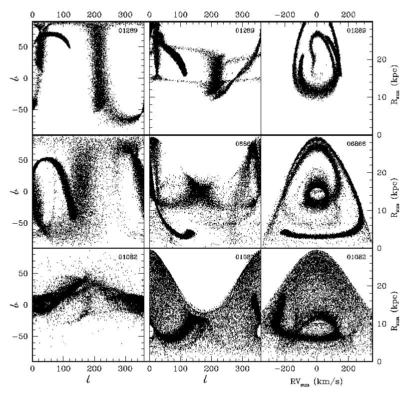
38