Introduction to Econometrics

Transcription

1 Introduction to Econometrics STAT-S-301 Introduction to Time Series Regression and Forecasting (2016/2017) Lecturer: Yves Dominicy Teaching Assistant: Elise Petit 1

2 Introduction to Time Series Regression and Forecasting Time series data are data collected on the same observational unit at multiple time periods: Aggregate consumption and GDP for a country (for example, 20 years of quarterly observations = 80 observations). Yen/$, pound/$ and Euro/$ exchange rates (daily data for 1 year = 365 observations). Cigarette consumption per capital in California, by year. 2

3 Example #1 of time series data: US rate of inflation 3

4 Example #2: US rate of unemployment 4

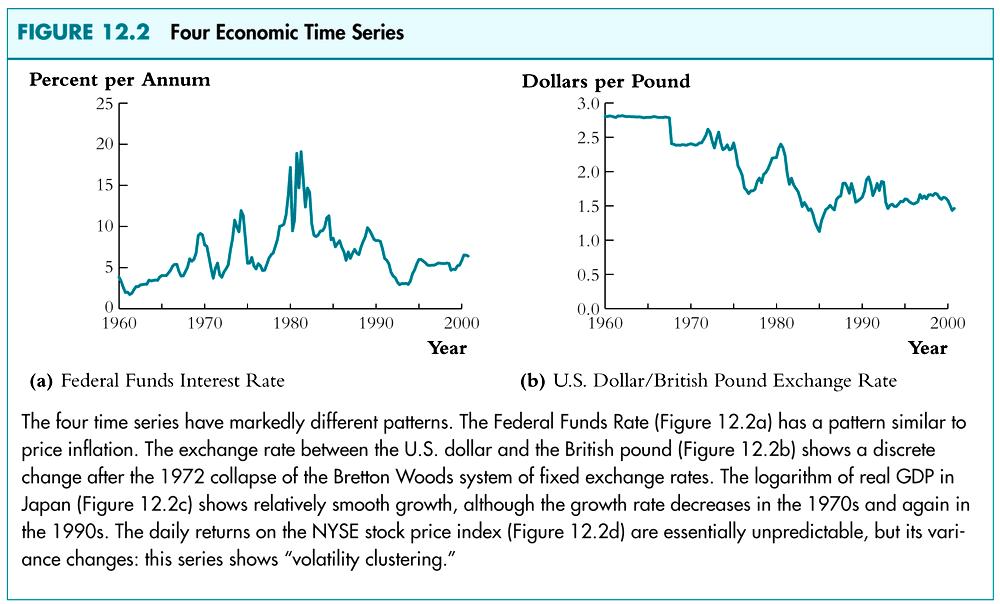
5 Why use time series data? To develop forecasting models: o What will the rate of inflation be next year? To estimate dynamic causal effects: o If the Fed increases the Federal Funds rate now, what will be the effect on the rates of inflation and unemployment in 3 months? in 12 months? o What is the effect over time on cigarette consumption of a hike in the cigarette tax. Modeling risks, which is used in financial markets, e.g. modeling changing variances and volatility clustering. Applications outside of economics include environmental and climate modeling, engineering, compuer science. 5

6 Time series data raises new technical issues Time lags. Correlation over time (serial correlation or autocorrelation, which we encountered in panel data). Forecasting models that have no causal interpretation (specialized tools for forecasting): o autoregressive (AR) models o autoregressive distributed lag (ADL) models. Conditions under which dynamic effects can be estimated, and how to estimate them. Calculation of standard errors when the errors are serially correlated. 6

7 Using Regression Models for Forecasting Forecasting and estimation of causal effects are quite different objectives. For forecasting, o 2 R matters (a lot!) o Omitted variable bias isn t a problem! o We will not worry about interpreting coefficients in forecasting models. o External validity is paramount: the model estimated using historical data must hold into the (near) future. 7

8 Notation for time series data Y t = value of Y in period t. Data set: Y 1,,Y T = T observations on the time series random variable Y. We consider only consecutive, evenly-spaced observations (for example, monthly, 1960 to 1999, no missing months) (else yet more complications...). 8

9 We will transform time series variables using lags, first differences, logarithms, & growth rates 9

10 Example: Quarterly rate of inflation at an annual rate CPI in the first quarter of 1999 (1999:I) = CPI in the second quarter of 1999 (1999:II) = Percentage change in CPI, 1999:I to 1999:II = = = 0.703%. Percentage change in CPI, 1999:I to 1999:II, at an annual rate = 4 x = 2.81% (percent per year). Like interest rates, inflation rates are (as a matter of convention) reported at an annual rate. Using the logarithmic approximation to percent changes yields 4 x100 x[log(166.03) log(164.87)] = 2.80%. 10

11 Example: US CPI inflation its first lag and its change CPI = Consumer price index (Bureau of Labor Statistics) 11

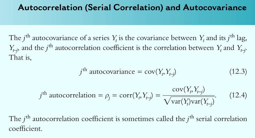
12 Autocorrelation The correlation of a series with its own lagged values is called autocorrelation or serial correlation. The first autocorrelation of Y t is corr(y t,y t 1 ). The first autocovariance of Y t is cov(y t,y t 1 ). Thus cov( Yt, Yt 1) corr(y t,y t 1 ) = = 1. var( Y ) var( Y ) t t 1 These are population correlations they describe the population joint distribution of (Y t,y t 1 ). 12

13 13

14 Example: Autocorrelations of: (1) the quarterly rate of U.S. inflation, (2) the quarter-to-quarter change in the quarterly rate of inflation. 14

15 The inflation rate is highly serially correlated ( 1 =.85). Last quarter s inflation rate contains much information about this quarter s inflation rate. The plot is dominated by multiyear swings. But there are still surprise movements! 15

16 16

17 17

18 Stationarity: a key idea for external validity of time series regression Stationarity says that the past is like the present and the future, at least in a probabilistic sense. We will focus on the case that Y t stationary. 18

19 Autoregressions A natural starting point for a forecasting model is to use past values of Y (that is, Y t 1, Y t 2, ) to forecast Y t. An autoregression is a regression model in which Y t is regressed against its own lagged values. The number of lags used as regressors is called the order of the autoregression. o In a first order autoregression, Y t is regressed against Y t 1. o In a p th order autoregression, Y t is regressed against Y t 1,Y t 2,,Y t p. The First Order Autoregressive (AR(1)) Model. 19

20 The population AR(1) model is Y t = Y t 1 + u t. 0 and 1 do not have causal interpretations. if 1 = 0, Y t 1 is not useful for forecasting Y t. The AR(1) model can be estimated by OLS regression of Y t against Y t 1. Testing 1 = 0 v. 1 0 provides a test of the hypothesis that Y t 1 is not useful for forecasting Y t. 20

21 Example: AR(1) model of the change in inflation Estimated using data from 1962:I 1999:IV. First, let STATA know you are using time series data generate time=q(1959q1)+_n-1; format time %tq; sort time; tsset time; _n is the observation no. So this command creates a new variable time that has a special quarterly date format. Specify the quarterly date format. Sort by time. Let STATA know that the variable time is the variable you want to indicate the time scale. 21

22 Example: AR(1) model of inflation STATA, ctd.. gen lcpi = log(cpi); variable cpi is already in memory.. gen inf = 400*(lcpi[_n]-lcpi[_n-1]); quarterly rate of inflation at an annual rate.. corrgram inf, noplot lags(8); computes first 8 sample autocorrelations LAG AC PAC Q Prob>Q gen inf = 400*(lcpi[_n]-lcpi[_n-1]) This syntax creates a new variable, inf, the nth observation of which is 400 times the difference between the nth observation on lcpi and the n- 1 th observation on lcpi, that is, the first difference of lcpi. 22

23 Example: AR(1) model of inflation STATA, ctd Syntax: L.dinf is the first lag of dinf. reg dinf L.dinf if tin(1962q1,1999q4), r; Regression with robust standard errors Number of obs = 152 F( 1, 150) = 3.96 Prob > F = R-squared = Root MSE = Robust dinf Coef. Std. Err. t P> t [95% Conf. Interval] dinf L _cons if tin(1962q1,1999q4) STATA time series syntax for using only observations between 1962q1 and 1999q4 (inclusive). This requires defining the time scale first, as we did above. 23

24 Forecasts and forecast errors A note on terminology: A predicted value refers to the value of Y predicted (using a regression) for an observation in the sample used to estimate the regression this is the usual definition. A forecast refers to the value of Y forecasted for an observation not in the sample used to estimate the regression. Predicted values are in sample. Forecasts are forecasts of the future which cannot have been used to estimate the regression. 24

25 Forecasts: notation Y t t 1 = forecast of Y t based on Y t 1,Y t 2,, using the population (true unknown) coefficients. Yˆtt 1= forecast of Y t based on Y t 1,Y t 2,, using the estimated coefficients, which were estimated using data through period t 1. For an AR(1), Y t t 1 = Y t 1 Y = ˆ 0 + ˆ 1Y t 1, where ˆ 0 and ˆ 1 were estimated ˆtt 1 using data through period t 1. 25

26 Forecast errors The one-period ahead forecast error is, forecast error = Y t Yˆtt 1. The distinction between a forecast error and a residual is the same as between a forecast and a predicted value: a residual is in-sample, a forecast error is out-of-sample the value of Y t isn t used in the estimation of the regression coefficients. 26

27 The root mean squared forecast error (RMSFE) RMSFE = E Y ˆ 2 [( t Yt t 1) ] The RMSFE is a measure of the spread of the forecast error distribution. The RMSFE is like the standard deviation of u t, except that it explicitly focuses on the forecast error using estimated coefficients, not using the population regression line. The RMSFE is a measure of the magnitude of a typical forecasting mistake. 27

28 Example: forecasting inflation using and AR(1) AR(1) estimated using data from 1962:I 1999:IV: Inf_est= Inf t 1 Inf 1999:III = 2.8 (units are percent, at an annual rate) Inf 1999:IV = 3.2 Inf 1999:IV = 0.4 So the forecast of Inf 2000:I is, Inf_est = x0.4 = so Inf_est = Inf 1999:IV + Inf_est = =

29 The p th order autoregressive model (AR(p)) Y t = Y t Y t p Y t p + u t The AR(p) model uses p lags of Y as regressors. The AR(1) model is a special case. The coefficients do not have a causal interpretation. To test the hypothesis that Y t 2,,Y t p do not further help forecast Y t, beyond Y t 1, use an F-test. Use t- or F-tests to determine the lag order p. Or, better, determine p using an information criterion. 29

30 Example: AR(4) model of inflation Inf_est = Inf t 1.32 Inf t Inf t 3 (.12) (.10) (.09) (.09).04 Inf t 4, (.10) 2 R = 0.21 F-statistic testing lags 2, 3, 4 is 6.43 (p-value <.001). 2 R increased from.04 to.21 by adding lags 2, 3, 4. Lags 2, 3, 4 (jointly) help to predict the change in inflation, above and beyond the first lag. 30

31 Example: AR(4) model of inflation STATA. reg dinf L(1/4).dinf if tin(1962q1,1999q4), r; Regression with robust standard errors Number of obs = 152 F( 4, 147) = 6.79 Prob > F = R-squared = Root MSE = Robust dinf Coef. Std. Err. t P> t [95% Conf. Interval] dinf L L L L _cons NOTES L(1/4).dinf is A convenient way to say use lags 1 4 of dinf as regressors. L1,,L4 refer to the first, second, 4 th lags of dinf. 31

32 . dis "Adjusted Rsquared = " _result(8); result(8) is the rbar-squared Adjusted Rsquared = of the most recently run regression.. test L2.dinf L3.dinf L4.dinf; L2.dinf is the second lag of dinf, etc. ( 1) L2.dinf = 0.0 ( 2) L3.dinf = 0.0 ( 3) L4.dinf = 0.0 F( 3, 147) = 6.43 Prob > F = Note: some of the time series features of STATA differ between STATA v. 7 and STATA v. 8 32

33 Digression: we used Inf, not Inf, in the AR s. Why? The AR(1) model of Inf t 1 is an AR(2) model of Inf t : or or so Inf t = Inf t 1 + u t Inf t Inf t 1 = (Inf t 1 Inf t 2 ) + u t Inf t = Inf t Inf t 1 1 Inf t 2 + u t Inf t = 0 + (1+ 1 )Inf t 1 1 Inf t 2 + u t 33

34 So why use Inf t, not Inf t? AR(1) model of Inf: AR(2) model of Inf: Inf t = Inf t 1 + u t Inf t = Inf t + 2 Inf t 1 + v t When Y t is strongly serially correlated, the OLS estimator of the AR coefficient is biased towards zero. In the extreme case that the AR coefficient = 1, Y t isn t stationary: the u t s accumulate and Y t blows up. If Y t isn t stationary, our regression theory are working with here breaks down. Here, Inf t is strongly serially correlated so to keep ourselves in a framework we understand, the regressions are specified using Inf. 34

35 Time Series Regression with Additional Predictors and the Autoregressive Distributed Lag (ADL) Model So far we have considered forecasting models that use only past values of Y. It makes sense to add other variables (X) that might be useful predictors of Y, above and beyond the predictive value of lagged values of Y: Y t = Y t p Y t p + 1 X t r X t r + u t. This is an autoregressive distributed lag (ADL) model. 35

36 Example: lagged unemployment and inflation According to the Phillips curve says that if unemployment is above its equilibrium, or natural, rate, then the rate of inflation will increase. That is, Inf t should be related to lagged values of the unemployment rate, with a negative coefficient. The rate of unemployment at which inflation neither increases nor decreases is often called the nonaccelerating rate of inflation unemployment rate: the NAIRU. Is this relation found in US economic data? Can this relation be exploited for forecasting inflation? 36

37 The empirical Phillips Curve The NAIRU is the value of u for which Inf = 0 37

38 Example: ADL(4,4) model of inflation Inf_est = Inf t 1.34 Inf t Inf t 3.03 Inf t 4 (.47) (.09) (.10) (.08) (.09) 2.68Unem t Unem t Unem t Unemp t 4 (.47) (.89) (.89) (.44) 2 R = 0.35 a big improvement over the AR(4), for which 2 R =.21 38

39 Example: dinf and unem STATA. reg dinf L(1/4).dinf L(1/4).unem if tin(1962q1,1999q4), r; Regression with robust standard errors Number of obs = 152 F( 8, 143) = 7.99 Prob > F = R-squared = Root MSE = Robust dinf Coef. Std. Err. t P> t [95% Conf. Interval] dinf L L L L unem L L L L _cons

40 Example: ADL(4,4) model of inflation STATA, ctd.. dis "Adjusted Rsquared = " _result(8); Adjusted Rsquared = test L2.dinf L3.dinf L4.dinf; ( 1) L2.dinf = 0.0 ( 2) L3.dinf = 0.0 ( 3) L4.dinf = 0.0 F( 3, 143) = 4.93 The extra lags of dinf are signif. Prob > F = test L1.unem L2.unem L3.unem L4.unem; ( 1) L.unem = 0.0 ( 2) L2.unem = 0.0 ( 3) L3.unem = 0.0 ( 4) L4.unem = 0.0 F( 4, 143) = 8.51 The lags of unem are significant Prob > F = The null hypothesis that the coefficients on the lags of the unemployment rate are all zero is rejected at the 1% significance level using the F- statistic. 40

41 The test of the joint hypothesis that none of the X s is a useful predictor, above and beyond lagged values of Y, is called a Granger causality test causality is an unfortunate term here: Granger Causality simply refers to (marginal) predictive content. 41

42 Summary: Time Series Forecasting Models For forecasting purposes, it isn t important to have coefficients with a causal interpretation! Simple and reliable forecasts can be produced using AR(p) models these are common benchmark forecasts against which more complicated forecasting models can be assessed. Additional predictors (X s) can be added; the result is an autoregressive distributed lag (ADL) model. Stationary means that the models can be used outside the range of data for which they were estimated. We now have the tools we need to estimate dynamic causal effects... 42