Chapter 11. Regression with a Binary Dependent Variable

Size: px

Start display at page:

Download "Chapter 11. Regression with a Binary Dependent Variable"

Jerome Waters
5 years ago
Views:

1 Chapter 11 Regression with a Binary Dependent Variable

2 2 Regression with a Binary Dependent Variable (SW Chapter 11) So far the dependent variable (Y) has been continuous: district-wide average test score traffic fatality rate What if Y is binary? Y = get into college, or not; X = years of education Y = person smokes, or not; X = income Y = mortgage application is accepted, or not; X = income, house characteristics, marital status, race

3 Example: Mortgage denial and race The Boston Fed HMDA data set Individual applications for single-family mortgages made in 1990 in the greater Boston area 2380 observations, collected under Home Mortgage Disclosure Act (HMDA) Variables Dependent variable: Is the mortgage denied or accepted? Independent variables: income, wealth, employment status other loan, property characteristics race of applicant 3

4 4 The Linear Probability Model (SW Section 11.1) A natural starting point is the linear regression model with a single regressor: Y i = β 0 + β 1 X i + u i But: ΔY What does β 1 mean when Y is binary? Is β 1 = Δ X? What does the line β 0 + β 1 X mean when Y is binary? What does the predicted value Y ˆ mean when Y is binary? For example, what does Y ˆ = 0.26 mean?

5 5 The linear probability model, ctd. Y i = β 0 + β 1 X i + u i Recall assumption #1: E(u i X i ) = 0, so E(Y i X i ) = E(β 0 + β 1 X i + u i X i ) = β 0 + β 1 X i When Y is binary, E(Y) = 1 Pr(Y=1) + 0 Pr(Y=0) = Pr(Y=1) so E(Y X) = Pr(Y=1 X)

6 The linear probability model, ctd. When Y is binary, the linear regression model Y i = β 0 + β 1 X i + u i is called the linear probability model. The predicted value is a probability: E(Y X=x) = Pr(Y=1 X=x) = prob. that Y = 1 given x Y ˆ = the predicted probability that Y i = 1, given X β 1 = change in probability that Y = 1 for a given Δx: Pr( 1 ) Pr( 1 ) β 1 = Y = X = x +Δ x Y = X = x Δx 6

7 7 Example: linear probability model, HMDA data Mortgage denial v. ratio of debt payments to income (P/I ratio) in the HMDA data set (subset)

8 8 Linear probability model: HMDA data, ctd. deny = P/I ratio (n = 2380) (.032) (.098) What is the predicted value for P/I ratio =.3? Pr( deny = 1 P / Iratio =.3) = =.151 Calculating effects: increase P/I ratio from.3 to.4: Pr( deny = 1 P / Iratio =.4) = =.212 The effect on the probability of denial of an increase in P/I ratio from.3 to.4 is to increase the probability by.061, that is, by 6.1 percentage points (what?).

9 9 Linear probability model: HMDA data, ctd Next include black as a regressor: deny = P/I ratio +.177black (.032) (.098) (.025) Predicted probability of denial: for black applicant with P/I ratio =.3: Pr( deny = 1) = =.254 for white applicant, P/I ratio =.3: Pr( deny = 1) = =.077 difference =.177 = 17.7 percentage points Coefficient on black is significant at the 5% level Still plenty of room for omitted variable bias

10 10 The linear probability model: Summary Models Pr(Y=1 X) as a linear function of X Advantages: simple to estimate and to interpret inference is the same as for multiple regression (need heteroskedasticity-robust standard errors) Disadvantages: Does it make sense that the probability should be linear in X? Predicted probabilities can be <0 or >1! These disadvantages can be solved by using a nonlinear probability model: probit and logit regression

11 11 Probit and Logit Regression (SW Section 11.2) The problem with the linear probability model is that it models the probability of Y=1 as being linear: Pr(Y = 1 X) = β 0 + β 1 X Instead, we want: 0 Pr(Y = 1 X) 1 for all X Pr(Y = 1 X) to be increasing in X (for β 1 >0) This requires a nonlinear functional form for the probability. How about an S-curve

12 12 The probit model satisfies these conditions: 0 Pr(Y = 1 X) 1 for all X Pr(Y = 1 X) to be increasing in X (for β 1 >0)

13 13 Probit regression models the probability that Y=1 using the cumulative standard normal distribution function, evaluated at z = β 0 + β 1 X: Pr(Y = 1 X) = Φ(β 0 + β 1 X) Φ is the cumulative normal distribution function. z = β 0 + β 1 X is the z-value or z-index of the probit model. Example: Suppose β 0 = -2, β 1 = 3, X =.4, so Pr(Y = 1 X=.4) = Φ( ) = Φ(-0.8) Pr(Y = 1 X=.4) = area under the standard normal density to left of z = -.8, which is

14 Pr(Z -0.8) =

15 15 Probit regression, ctd. Why use the cumulative normal probability distribution? The S-shape gives us what we want: 0 Pr(Y = 1 X) 1 for all X Pr(Y = 1 X) to be increasing in X (for β 1 >0) Easy to use the probabilities are tabulated in the cumulative normal tables Relatively straightforward interpretation: z-value = β 0 + β 1 X ˆ β 0 + ˆ β 1 X is the predicted z-value, given X β 1 is the change in the z-value for a unit change in X

16 STATA Example: HMDA data. probit deny p_irat, r; Iteration 0: log likelihood = Iteration 1: log likelihood = Iteration 2: log likelihood = Iteration 3: log likelihood = We ll discuss this later Probit estimates Number of obs = 2380 Wald chi2(1) = Prob > chi2 = Log likelihood = Pseudo R2 = Robust deny Coef. Std. Err. z P> z [95% Conf. Interval] p_irat _cons Pr( deny = 1 P / Iratio) = Φ( P/I ratio) (.16) (.47) 16

17 STATA Example: HMDA data, ctd. Pr( deny = 1 P / Iratio) = Φ( P/I ratio) (.16) (.47) Positive coefficient: does this make sense? Standard errors have the usual interpretation Predicted probabilities: Pr( deny = 1 P / Iratio =.3) = Φ( ) = Φ(-1.30) =.097 Effect of change in P/I ratio from.3 to.4: Pr( deny = 1 P / Iratio =.4) = Φ( ) =.159 Predicted probability of denial rises from.097 to

18 18 Probit regression with multiple regressors Pr(Y = 1 X 1, X 2 ) = Φ(β 0 + β 1 X 1 + β 2 X 2 ) Φ is the cumulative normal distribution function. z = β 0 + β 1 X 1 + β 2 X 2 is the z-value or z-index of the probit model. β 1 is the effect on the z-score of a unit change in X 1, holding constant X 2

19 19 STATA Example: HMDA data. probit deny p_irat black, r; Iteration 0: log likelihood = Iteration 1: log likelihood = Iteration 2: log likelihood = Iteration 3: log likelihood = Probit estimates Number of obs = 2380 Wald chi2(2) = Prob > chi2 = Log likelihood = Pseudo R2 = Robust deny Coef. Std. Err. z P> z [95% Conf. Interval] p_irat black _cons We ll go through the estimation details later

20 STATA Example, ctd.: predicted probit probabilities. probit deny p_irat black, r; Probit estimates Number of obs = 2380 Wald chi2(2) = Prob > chi2 = Log likelihood = Pseudo R2 = Robust deny Coef. Std. Err. z P> z [95% Conf. Interval] p_irat black _cons sca z1 = _b[_cons]+_b[p_irat]*.3+_b[black]*0;. display "Pred prob, p_irat=.3, white: " normprob(z1); Pred prob, p_irat=.3, white: NOTE _b[_cons] is the estimated intercept ( ) _b[p_irat] is the coefficient on p_irat ( ) sca creates a new scalar which is the result of a calculation display prints the indicated information to the screen 20

21 21 STATA Example, ctd. Pr( deny = 1 P / I, black) = Φ( P/I ratio +.71 black) (.16) (.44) (.08) Is the coefficient on black statistically significant? Estimated effect of race for P/I ratio =.3: Pr( deny = 1.3,1) = Φ( ) =.233 Pr( deny = 1.3,0) = Φ( ) =.075 Difference in rejection probabilities =.158 (15.8 percentage points) Still plenty of room still for omitted variable bias

22 Logit Regression Logit regression models the probability of Y=1 as the cumulative standard logistic distribution function, evaluated at z = β 0 + β 1 X: Pr(Y = 1 X) = F(β 0 + β 1 X) F is the cumulative logistic distribution function: F(β 0 + β 1 X) = 1+ 1 ( 0 1X ) e β + β 22

23 Logit regression, ctd. Pr(Y = 1 X) = F(β 0 + β 1 X) where F(β 0 + β 1 X) = 1+ 1 ( 0 1X ) e β + β. Example: β 0 = -3, β 1 = 2, X =.4, so β 0 + β 1 X = = -2.2 so Pr(Y = 1 X=.4) = 1/(1+e ( 2.2) ) =.0998 Why bother with logit if we have probit? Historically, logit is more convenient computationally In practice, logit and probit are very similar 23

24 24 STATA Example: HMDA data. logit deny p_irat black, r; Iteration 0: log likelihood = Later Iteration 1: log likelihood = Iteration 2: log likelihood = Iteration 3: log likelihood = Iteration 4: log likelihood = Logit estimates Number of obs = 2380 Wald chi2(2) = Prob > chi2 = Log likelihood = Pseudo R2 = Robust deny Coef. Std. Err. z P> z [95% Conf. Interval] p_irat black _cons dis "Pred prob, p_irat=.3, white: " > 1/(1+exp(-(_b[_cons]+_b[p_irat]*.3+_b[black]*0))); Pred prob, p_irat=.3, white: NOTE: the probit predicted probability is

25 Predicted probabilities from estimated probit and logit models usually are (as usual) very close in this application. 25

26 26 Example for class discussion: Characterizing the Background of Hezbollah Militants Source: Alan Krueger and Jitka Maleckova, Education, Poverty and Terrorism: Is There a Causal Connection? Journal of Economic Perspectives, Fall 2003, Logit regression: 1 = died in Hezbollah military event Table of logit results:

27 27

28 28

29 29 Hezbollah militants example, ctd. Compute the effect of schooling by comparing predicted probabilities using the logit regression in column (3): Pr(Y=1 secondary = 1, poverty = 0, age = 20) Pr(Y=0 secondary = 0, poverty = 0, age = 20): Pr(Y=1 secondary = 1, poverty = 0, age = 20) = 1/[1+e ( ) ] = 1/[1 + e ] = does this make sense? Pr(Y=1 secondary = 0, poverty = 0, age = 20) = 1/[1+e ( ) ] = 1/[1 + e ] = does this make sense?

30 30 Predicted change in probabilities: Pr(Y=1 secondary = 1, poverty = 0, age = 20) Pr(Y=1 secondary = 1, poverty = 0, age = 20) = = Both these statements are true: The probability of being a Hezbollah militant increases by percentage points, if secondary school is attended. The probability of being a Hezbollah militant increases by 32%, if secondary school is attended ( / =.32). These sound so different! what is going on?

31 31 Estimation and Inference in Probit (and Logit) Models (SW Section 11.3) Probit model: Pr(Y = 1 X) = Φ(β 0 + β 1 X) Estimation and inference How can we estimate β 0 and β 1? What is the sampling distribution of the estimators? Why can we use the usual methods of inference? First motivate via nonlinear least squares Then discuss maximum likelihood estimation (what is actually done in practice)

32 Probit estimation by nonlinear least squares Recall OLS: n min [ Y ( b + b X )] b0, b1 i 0 1 i i= 1 The result is the OLS estimators ˆ β 0 and ˆ β 1 Nonlinear least squares estimator of probit coefficients: n min [ Y Φ ( b + b X )] b0, b1 i 0 1 i i= 1 How to solve this minimization problem? Calculus doesn t give and explicit solution. Solved numerically using the computer(specialized minimization algorithms) In practice, nonlinear least squares isn t used because it isn t efficient an estimator with a smaller variance is

33 33 Probit estimation by maximum likelihood The likelihood function is the conditional density of Y 1,,Y n given X 1,,X n, treated as a function of the unknown parameters β 0 and β 1. The maximum likelihood estimator (MLE) is the value of (β 0, β 1 ) that maximize the likelihood function. The MLE is the value of (β 0, β 1 ) that best describe the full distribution of the data. In large samples, the MLE is: consistent normally distributed efficient (has the smallest variance of all estimators)

34 34 Special case: the probit MLE with no X Y = 1 with probability p 0 with probability 1 p (Bernoulli distribution) Data: Y 1,,Y n, i.i.d. Derivation of the likelihood starts with the density of Y 1 : so Pr(Y 1 = 1) = p and Pr(Y 1 = 0) = 1 p y1 1 y1 Pr(Y 1 = y 1 ) = p (1 p) (verify this for y 1 =0, 1!)

35 35 Joint density of (Y 1,Y 2 ): Because Y 1 and Y 2 are independent, Pr(Y 1 = y 1,Y 2 = y 2 ) = Pr(Y 1 = y 1 ) Pr(Y 2 = y 2 ) y1 1 y1 = [ p (1 p) y2 1 y2 ] [ p (1 p) ] = Joint density of (Y 1,..,Y n ): p ( y + y ) [ 2 ( y + y )] (1 p) Pr(Y 1 = y 1,Y 2 = y 2,,Y n = y n ) y1 1 y1 = [ p (1 p) y2 1 y2 ] [ p (1 p) ] [ n n y ( n y 1 i ) i 1 i i = p = = (1 p) p y n (1 ) 1 yn p ]

36 36 The likelihood is the joint density, treated as a function of the unknown parameters, which here is p: ( ) n n Y n Y 1 i i 1 i i f(p;y 1,,Y n ) = p = = (1 p) The MLE maximizes the likelihood. Its easier to work with the logarithm of the likelihood, ln[f(p;y 1,,Y n )]: ln[f(p;y 1,,Y n )] = ( n ) ( n ) i i Y ln( p) + n Y ln(1 p) i= 1 i= 1 Maximize the likelihood by setting the derivative = 0: dln f( p; Y1,..., Y n ) = ( n ) 1 ( n ) 1 Y i 1 i + n Y = i= 1 i dp p 1 p Solving for p yields the MLE; that is, p ˆ MLE satisfies, = 0

37 37 or or or MLE pˆ 1 pˆ ( n ) ( n Y ) 1 i n Y i= MLE i= 1 i = pˆ 1 pˆ ( n ) ( n Y ) 1 i = n Y i= MLE i= 1 i Y pˆ = 1 Y 1 pˆ MLE MLE MLE ˆ MLE p = Y = fraction of 1 s whew a lot of work to get back to the first thing you would think of using but the nice thing is that this whole approach generalizes to more complicated models...

38 38 The MLE in the no-x case (Bernoulli distribution), ctd.: ˆ MLE p = Y = fraction of 1 s For Y i i.i.d. Bernoulli, the MLE is the natural estimator of p, the fraction of 1 s, which is Y We already know the essentials of inference: In large n, the sampling distribution of p ˆ MLE = Y is normally distributed Thus inference is as usual: hypothesis testing via t- statistic, confidence interval as ± 1.96SE

39 39 The MLE in the no-x case (Bernoulli distribution), ctd: The theory of maximum likelihood estimation says that p ˆ MLE is the most efficient estimator of p of all possible estimators at least for large n. (Much stronger than the Gauss-Markov theorem). This is why people use the MLE. STATA note: to emphasize requirement of large-n, the printout calls the t-statistic the z-statistic; instead of the F- statistic, the chi-squared statistic (= q F). Now we extend this to probit in which the probability is conditional on X the MLE of the probit coefficients.

40 40 The probit likelihood with one X The derivation starts with the density of Y 1, given X 1 : Pr(Y 1 = 1 X 1 ) = Φ(β 0 + β 1 X 1 ) Pr(Y 1 = 0 X 1 ) = 1 Φ(β 0 + β 1 X 1 ) so y1 1 y1 Pr(Y 1 = y 1 X 1 ) = Φ ( β + β X ) [1 Φ ( β + β X )] The probit likelihood function is the joint density of Y 1,,Y n given X 1,,X n, treated as a function of β 0, β 1 : f(β 0,β 1 ; Y 1,,Y n X 1,,X n ) Y1 1 = { ( ) [1 ( )] 1 Y Φ β + β X Φ β + β X } Yn 1 Yn { Φ ( β + β X ) [1 Φ ( β + β X )] } 0 1 n 0 1 n

41 41 The probit likelihood function: f(β 0,β 1 ; Y 1,,Y n X 1,,X n ) Y1 1 Y1 = { Φ ( β + β X ) [1 Φ ( β + β X )] } Yn 1 Yn { Φ ( β + β X ) [1 Φ ( β + β X )] } 0 1 n 0 1 Can t solve for the maximum explicitly Must maximize using numerical methods As in the case of no X, in large samples: ˆ MLE 0 ˆ MLE 0 ˆ MLE 0 ˆ MLE β, β 1 are consistent β, ˆ β MLE 1 are normally distributed β, ˆ β MLE 1 are asymptotically efficient among all estimators (assuming the probit model is the correct model) n

42 42 The Probit MLE, ctd. Standard errors of ˆ β MLE 0, ˆ β MLE 1 are computed automatically Testing, confidence intervals proceeds as usual For multiple X s, see SW App. 11.2

43 43 The logit likelihood with one X The only difference between probit and logit is the functional form used for the probability: Φ is replaced by the cumulative logistic function. Otherwise, the likelihood is similar; for details see SW App As with probit, ˆ β MLE 0, ˆ β MLE 1 are consistent ˆ β MLE 0, ˆ β MLE 1 are normally distributed Their standard errors can be computed Testing, confidence intervals proceeds as usual

44 44 Measures of fit for logit and probit The R 2 2 and R don t make sense here (why?). So, two other specialized measures are used: 1. The fraction correctly predicted = fraction of Y s for which predicted probability is >50% (if Y i =1) or is <50% (if Y i =0). 2. The pseudo-r 2 measure the fit using the likelihood function: measures the improvement in the value of the log likelihood, relative to having no X s (see SW App. 11.2). This simplifies to the R 2 in the linear model with normally distributed errors.

45 45 Application to the Boston HMDA Data (SW Section 11.4) Mortgages (home loans) are an essential part of buying a home. Is there differential access to home loans by race? If two otherwise identical individuals, one white and one black, applied for a home loan, is there a difference in the probability of denial?

46 46 The HMDA Data Set Data on individual characteristics, property characteristics, and loan denial/acceptance The mortgage application process circa : Go to a bank or mortgage company Fill out an application (personal+financial info) Meet with the loan officer Then the loan officer decides by law, in a race-blind way. Presumably, the bank wants to make profitable loans, and the loan officer doesn t want to originate defaults.

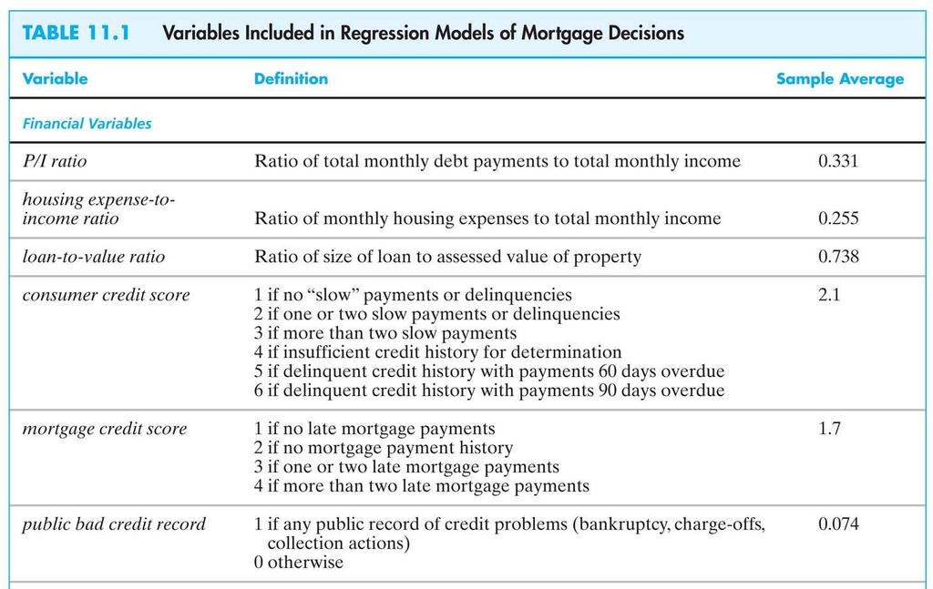
47 47 The loan officer s decision Loan officer uses key financial variables: P/I ratio housing expense-to-income ratio loan-to-value ratio personal credit history The decision rule is nonlinear: loan-to-value ratio > 80% loan-to-value ratio > 95% (what happens in default?) credit score

48 48 Regression specifications Pr(deny=1 black, other X s) = linear probability model probit Main problem with the regressions so far: potential omitted variable bias. All these (i) enter the loan officer decision function, all (ii) are or could be correlated with race: wealth, type of employment credit history family status The HMDA data set is very rich

49 49

50 50

51 51

52 Table 11.2, ctd. 52

53 Table 11.2, ctd. 53

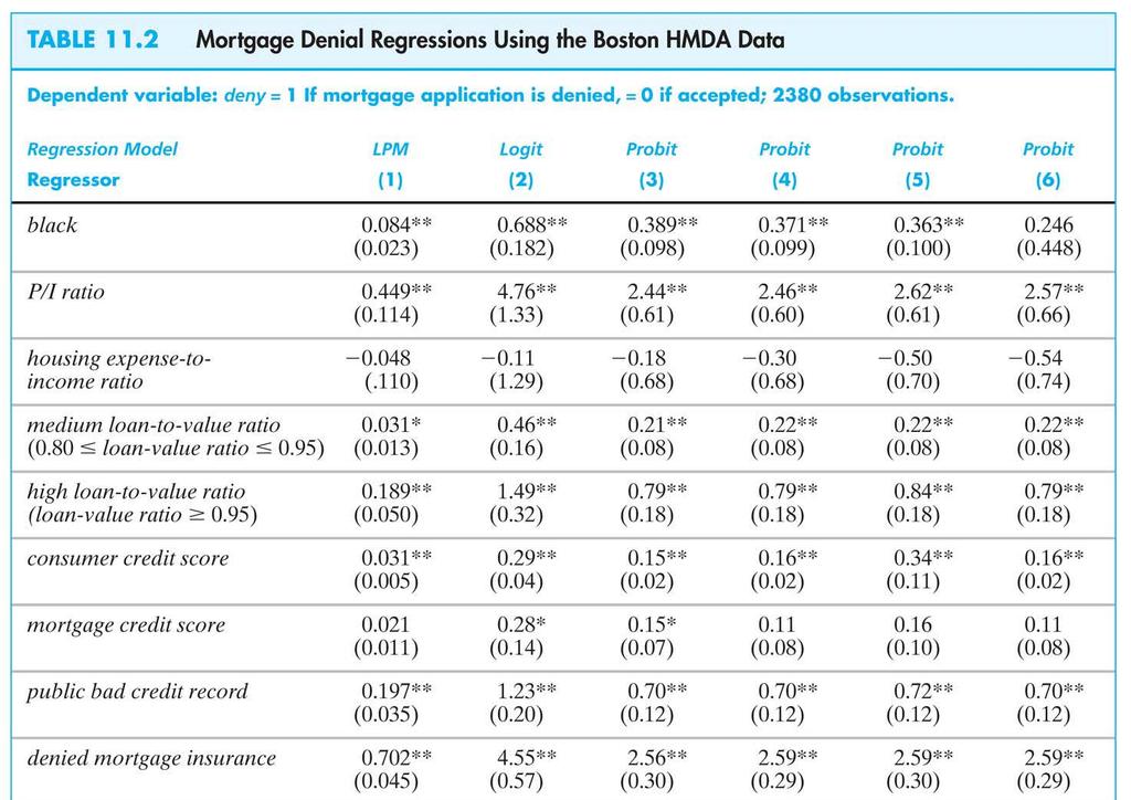
54 54 Summary of Empirical Results Coefficients on the financial variables make sense. Black is statistically significant in all specifications Race-financial variable interactions aren t significant. Including the covariates sharply reduces the effect of race on denial probability. LPM, probit, logit: similar estimates of effect of race on the probability of denial. Estimated effects are large in a real world sense.

55 55 Remaining threats to internal, external validity Internal validity 1. omitted variable bias what else is learned in the in-person interviews? 2. functional form misspecification (no ) 3. measurement error (originally, yes; now, no ) 4. selection random sample of loan applications define population to be loan applicants 5. simultaneous causality (no) External validity This is for Boston in What about today?

56 56 Summary (SW Section 11.5) If Y i is binary, then E(Y X) = Pr(Y=1 X) Three models: linear probability model (linear multiple regression) probit (cumulative standard normal distribution) logit (cumulative standard logistic distribution) LPM, probit, logit all produce predicted probabilities Effect of ΔX is change in conditional probability that Y=1. For logit and probit, this depends on the initial X Probit and logit are estimated via maximum likelihood Coefficients are normally distributed for large n Large-n hypothesis testing, conf. intervals is as usual

Binary Dependent Variable. Regression with a

Binary Dependent Variable. Regression with a Beykent University Faculty of Business and Economics Department of Economics Econometrics II Yrd.Doç.Dr. Özgür Ömer Ersin Regression with a Binary Dependent Variable (SW Chapter 11) SW Ch. 11 1/59 Regression