Question 1 [17 points]: (ch 11)

Transcription

1 Question 1 [17 points]: (ch 11) A study analyzed the probability that Major League Baseball (MLB) players "survive" for another season, or, in other words, play one more season. They studied a model of the following form: The dependent variable is a binary variable that takes on a value of one if the player played one more season (a minimum of 50 at bats or 25 innings pitched), and zero otherwise. Seasons is the number of total seasons played, measured in years, Perf is the performance of the player this year, and Avgperf is the average performance of the player over their career. The researchers had a sample of 4,728 hitters and 3,803 pitchers for the years All explanatory variables are standardized (sample mean of 0, variance of 1). Probit estimation yielded the results as shown in the table: Regression (1) Hitters (2) Pitchers Regression model probit probit constant (0.030) (0.031) number of seasons played (0.004) (0.005) performance (0.025) (0.026) average performance (0.033) (0.036) (a) (6p) Interpret the two probit equations and calculate survival probabilities for hitters and pitchers at the sample mean. Provide an explanation for why these are so high. (b) (6p) Calculate the change in the survival probability for a player who has a very bad year by performing two standard deviations below the average (assume also that this player has been in the majors for many years so that his average performance is negligibly affected). How does this change the survival probability when compared to the answer in (a)? (c) (5p) Since the results for hitters and pitchers seem similar, the researcher could consider combining the two samples. With a combined sample, how could you test the hypothesis that the coefficients for the explanatory variables are the same for hitters and pitchers? Explain in some detail.. Answer: (a) Note that all variables are standardized, so that the mean is zero. This results in a survival probability of for hitters and for pitchers. These results are so 2

2 high because there is a high probability, in general, for a player to return the following season. (b) Since the variables are standardized, this implies a change of two for the performance variable. The result for hitters is a lowering of the survival probability to 0.65, and for pitchers to (c) After combining the sample for hitters and pitchers, you would allow for a different intercept and slopes by introducing a binary variable for pitchers if hitters are the default. This binary variable would be introduced by itself and in combination with each of the above variables, thereby allowing all coefficients to differ. You could then conduct an F-test for the joint hypothesis that all coefficients involving the binary variables are zero. If the hypothesis cannot be rejected, then there is no difference between the coefficients for hitters and pitchers. 3

3 Question 2 [21 points]: (ch 10) Consider the following panel data regression with a single explanatory variable Yit = β0 + β1xit +. In each of the examples below, you will be including entity and time fixed effects. (a) (3 p) Consider the effect of beer taxes on the fatality rate using annual data from , and nine U.S. regions (New England, Pacific, Mid-Atlantic, South, etc.). How many total coefficients do you need to estimate? (b) (4 p) Certain regions (e.g. New England) that tend to have higher beer taxes also tend to have consistently higher quality hospitals. Does this pose a threat to your analysis? (c) (3 p) Consider the effect of the minimum wage on teenage employment using annual data from for five Canadian Regions (Atlantic Provinces, Quebec, Ontario, Prairies, British Columbia). How many total coefficients do you need to estimate? (d) (4 p) Nationwide recessions impact both teenage employment and the minimum wage across the country. Does this pose a threat to your analysis? (e) (3 p) Consider the effect of savings rates on per capita income using data for three decades ( , , ; one observation per decade) and 104 countries. How many total coefficients do you need to estimate? (f) (4 p) A number of countries industrialized at different times between , a process which can impact both the savings rate and per capita income. Does this pose a threat to your analysis? Answer: (a) 16 coefficients (6 time fixed effects, 8 entity fixed effects, intercept, slope). (b) No, entity fixed effects will account for entity constant omitted variables. (c) 43 coefficients (37 time fixed effects, 5 entity fixed effects, intercept, slope). (d) No, time fixed effects will account for this. (e) 107 coefficients (3 time fixed effects, 103 entity fixed effects, intercept, slope). (f) Yes, industrialization is a time and entity varying omitted variable. 4

4 Question 3 [15 points]: (IV regression) (Ch 12) Consider a supply model for edible chicken, which the the U.S. Department of Agriculture calls broilers Data for this question is adapted from the data provided by Epple and McCallum (2006) 1. The data are annual, The Supply equation is: ( ) ( ) ( ) ( ) where is aggregate production of young chickens, is the real price index of fresh chicken, is real price index of broiler feed, and which is included to capture any technical progress in the production. Some potential external instrumental variables are ( ), where is the real per capita income; ( ), where is the real price of beef; is the percent population growth from year t-1 to year t; ( ) is the lagged log of real price of chickens; ( ) is the log of exports of chicken. Estimated supply equation for chicken can be written from the following output: Regression 1:. reg lnqprod lnp lnpf TIME lnqprod_1 Source SS df MS Number of obs = F( 4, 35) = Model Prob > F = Residual R-squared = Adj R-squared = Total Root MSE = lnqprod Coef. Std. Err. t P> t [95% Conf. Interval] lnp lnpf TIME lnqprod_ _cons Regression 2:. ivreg lnqprod (lnp=lnpb lny POPGRO lnexpts) lnpf TIME lnqprod_1 Instrumental variables (2SLS) regression Source SS df MS Number of obs = F( 4, 35) = Model Prob > F = Residual R-squared = Adj R-squared = Total Root MSE = Simultaneous Equation Econometrics: The Missing Example, Economic Inquiry, 44(2),

5 lnqprod Coef. Std. Err. t P> t [95% Conf. Interval] lnp lnpf TIME lnqprod_ _cons Instrumented: lnp Instruments: lnpf TIME lnqprod_1 lnpb lny POPGRO lnexpts Regression 3:. reg lnp lnpb lny POPGRO lnexpts lnpf TIME lnqprod_1 Source SS df MS Number of obs = F( 7, 32) = Model Prob > F = Residual R-squared = Adj R-squared = Total Root MSE = lnp Coef. Std. Err. t P> t [95% Conf. Interval] lnpb lny POPGRO lnexpts lnpf TIME lnqprod_ _cons c Regression 4:. reg lnqprod lnp lnpf TIME lnqprod_1 Source SS df MS Number of obs = F( 4, 35) = Model Prob > F = Residual R-squared = Adj R-squared = Total Root MSE = lnqprod Coef. Std. Err. t P> t [95% Conf. Interval] lnp lnpf TIME lnqprod_ _cons

6 . predict e, residuals (1 missing values generated) Regression 5:. reg e lnpb lny POPGRO lnexpts lnpf TIME lnqprod_1 Source SS df MS Number of obs = F( 7, 32) = 2.19 Model Prob > F = Residual R-squared = Adj R-squared = Total Root MSE = e Coef. Std. Err. t P> t [95% Conf. Interval] lnpb lny POPGRO lnexpts lnpf TIME lnqprod_ _cons test lnpb lny POPGRO lnexpts ( 1) lnpb = 0 ( 2) lny = 0 ( 3) POPGRO = 0 ( 4) lnexpts = 0 F( 4, 32) = 3.83 Prob > F = (a) (4p) Compare the results in regression 1 and 2. Explain the reasons for instrumental variables in regression 2? Answer: (b) (5p) What are the requirements for valid instruments? Explain with mathematical conditions. Answer: 7

7 Relevance: ( ) Exogeneity: ( ) (c) (6p) Do these instruments satisfy the requirements? You must use the necessary regression results for your answer. Please specify the regression number you use while answering each part of this questions. (1) Relevancy: Using regression 3, square of t test is greater than 10 only for lnexprt, that is the only relevant IV. (2) Exogeneity: ( ) Hence, reject Therefore IV are not exogeneous. 8

8 Question 4 [15 points]: (Ch 15) There is some economic research that suggests that oil prices play a central role in causing recessions in developed countries. In particular, this research suggests that it is specifically increases in oil prices that matter. As a result, economists often look only at the percentage point difference between oil prices at date t and the maximum value over the previous year. However, you notice that energy prices can fluctuate quite dramatically in both directions and believe that geographic areas also benefit substantially from oil price decreases. As a result, you decide to consider the effect of real oil prices (Poil/CPI) on GDP growth (Yt) You estimate the following distributed lag model using annual data (numbers in parenthesis are HAC standard errors): t = (Poil/CPI)t (Poil/CPI)t-1 (0.27) (0.010) (0.011) t = , R2 = 0.15, SER = 1.88 (a) (5p) What is the impact effect of a 25 percentage point increase in real oil prices? (b) (5p) What is the predicted cumulative change in GDP Growth over two years of this effect? (c) (5p) The HAC F-statistic is Can you reject the null hypothesis that oil price changes have no effect on real GDP growth? What is the critical value you considered? Is there any reason why you should be cautious using an F-test in this case, given the sample period? Answer: a. GDP growth would decrease by almost a quarter of a percentage point. b. The predicted decline in growth would be almost one percentage point (-0.925). c. The critical value of F2, = 3.00 at the 5% significance level. Hence you can reject the null hypothesis that oil prices have no effect on real GDP growth. However, since the sample period involves only 50 or so observations, it is not clear that the test statistic is actually F-distributes (small sample). 9

9 Question 5 [20 points]: (Ch 14) Given the following STATA output, you can find a VAR(2) (VectorAutoregression) model of change in inflation ( ) and unemployment rate ( ). var unem cinf Vector autoregression Sample: No. of obs = 62 Log likelihood = AIC = FPE = HQIC = Det(Sigma_ml) = SBIC = Equation Parms RMSE R-sq chi2 P>chi unem cinf Coef. Std. Err. z P> z [95% Conf. Interval] unem unem L L cinf L L _cons cinf unem L L cinf L L _cons Table 1 Year Unem Inflation (a) (4p) Given the actual realizations of unemployment and inflation in table 1, forecast unemployment for 2013, show your work 10

10 (b) (4p) Given the actual realizations of unemployment and inflation in table 1, forecast inflation for 2013, show your work (c) (4p) Following is the joint test result for the second lags of unemployment rate and the inflation rate, according to the following test, would a VAR(1) model be better forecasting model than a VAR(2) model, explain why?. test L2.cinf L2.unem ( 1) [unem]l2.cinf = 0 ( 2) [cinf]l2.cinf = 0 ( 3) [unem]l2.unem = 0 ( 4) [cinf]l2.unem = 0 chi2( 4) = Prob > chi2 = (d) (4p) Why might a researcher use change in inflation as opposed to inflation in this model? Explain. (e) (4p) Should one use change in unemployment instead of unemployment? Explain. 11

11 Question 6 [12 points]: (Derivation question) Consider the panel data model: where are i.i.d. and independent of Xs with mean zero and variance, (a) (3 p) Define and, the entity demeaned values of X and Y. (b) (3 p) Rewrite the model in terms of these demeaned variables. (c) (3 p) Derive algebraically the fixed-effects estimator of. The fixed effects estimator minimizes the sum of squared residuals of the model you wrote in part b. (d) (3 p) Show that, if is a random variable that is independent of X and u, the estimator is unbiased for. Explain your answer. Answer: (a) (b) (c) 12

12 Subtracting the last equation from the first we would get; ( ) or we can also write it as; (d) The fixed-effects estimator of is the OLS estimator of the above regression. ( ) ( ) Hence, Using We can write ( ) Since is independent of X s and U s, using Law of Iterated Expectations we can show that [ ] 13

13 Bonus Question [2 points]: The two conditions for instrument validity are corr(zi, Xi) 0 and corr(zi, ui) = 0. The reason for the inconsistency of OLS is that corr(xi, ui) 0. If X and Z are correlated, and X and u are also correlated, how is it possible that Z and u are not correlated? Explain. Answer: The major idea is that corr(xi, ui) has two parts: one for which the correlation is zero and a second for which it is non-zero. The trick is to isolate the uncorrelated part of X. For the instrument to be valid, corr(zi, ui) = 0 and corr(zi, Xi) 0 must hold. TSLS then generates predicted values of X in the first stage by using a linear combination of the instruments. As long as corr(zi, Xi) 0 and corr(zi, ui) = 0, then the part of X which is uncorrelated with the error term is extracted through the prediction. In the second stage, this captured exogenous variation in X is then used to estimate the effect of X on Y, which is exogenous. 14

14 Selected Tables from Stock and Watson, Introduction to Econometrics 15

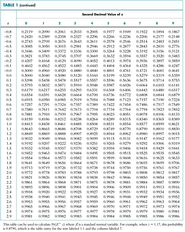
15 16

16 17

17 18