Econ 423 Lecture Notes

Transcription

1 Econ 423 Lecture Notes (These notes are slightly modified versions of lecture notes provided by Stock and Watson, They are for instructional purposes only and are not to be distributed outside of the classroom.) 14-1

2 Introduction to Time Series Regression and Forecasting Time series data are data collected on the same observational unit at multiple time periods Aggregate consumption and GDP for a country (for example, 20 years of quarterly observations = 80 observations) Yen/$, pound/$ and Euro/$ exchange rates (daily data for 1 year = 365 observations) Cigarette consumption per capita in a state, by year 14-2

3 Example #1 of time series data: US rate of price inflation, as measured by the quarterly percentage change in the Consumer Price Index (CPI), at an annual rate 14-3

4 Example #2: US rate of unemployment 14-4

5 Why use time series data? To develop forecasting models o What will the rate of inflation be next year? To estimate dynamic causal effects o If the Fed increases the Federal Funds rate now, what will be the effect on the rates of inflation and unemployment in 3 months? in 12 months? o What is the effect over time on cigarette consumption of a hike in the cigarette tax? Or, because that is your only option o Rates of inflation and unemployment in the US can be observed only over time! 14-5

6 Time series data raises new technical issues Time lags Correlation over time (serial correlation, a.k.a. autocorrelation) Forecasting models built on regression methods: o autoregressive (AR) models o autoregressive distributed lag (ADL) models o need not (typically do not) have a causal interpretation Conditions under which dynamic effects can be estimated, and how to estimate them Calculation of standard errors when the errors are serially correlated 14-6

7 Using Regression Models for Forecasting Forecasting and estimation of causal effects are quite different objectives. For forecasting, o 2 R matters (a lot!) o Omitted variable bias isn t a problem! o We will not worry about interpreting coefficients in forecasting models o External validity is paramount: the model estimated using historical data must hold into the (near) future 14-7

8 Introduction to Time Series Data and Serial Correlation First, some notation and terminology. Notation for time series data Y t = value of Y in period t. Data set: Y 1,,Y T = T observations on the time series random variable Y We consider only consecutive, evenly-spaced observations (for example, monthly, 1960 to 1999, no missing months) (missing and non-evenly spaced data introduce technical complications) 14-8

9 We will transform time series variables using lags, first differences, logarithms, & growth rates 14-9

10 Example: Quarterly rate of inflation at an annual rate (U.S.) CPI = Consumer Price Index (Bureau of Labor Statistics) CPI in the first quarter of 2004 (2004:I) = CPI in the second quarter of 2004 (2004:II) = Percentage change in CPI, 2004:I to 2004:II = = = 1.088% Percentage change in CPI, 2004:I to 2004:II, at an annual rate = = 4.359% 4.4% (percent per year) Like interest rates, inflation rates are (as a matter of convention) reported at an annual rate. Using the logarithmic approximation to percent changes yields [log(188.60) log(186.57)] = 4.329% 14-10

11 Example: US CPI inflation its first lag and its change 14-11

12 Autocorrelation The correlation of a series with its own lagged values is called autocorrelation or serial correlation. The first autocorrelation of Y t is corr(y t,y t 1 ) The first autocovariance of Y t is cov(y t,y t 1 ) Thus cov( Yt, Yt 1) corr(y t,y t 1 ) = =ρ 1 var( Y ) var( Y ) t t 1 These are population correlations they describe the population joint distribution of (Y t, Y t 1 ) 14-12

13 14-13

14 Sample autocorrelations The j th sample autocorrelation is an estimate of the j th population autocorrelation: cov( Yt, Yt j ) ˆ ρ j = var( Y ) where T 1 cov( Yt, Yt j ) = ( Yt Y j+ 1, T )( Yt j Y1, T j ) T t= j+ 1 where Y j + 1, T is the sample average of Y t computed over observations t = j+1,,t. NOTE: o the summation is over t=j+1 to T (why?) o The divisor is T, not T j (this is the conventional definition used for time series data) t 14-14

15 Example: Autocorrelations of: (1) the quarterly rate of U.S. inflation (2) the quarter-to-quarter change in the quarterly rate of inflation 14-15

16 The inflation rate is highly serially correlated (ρ 1 =.84) Last quarter s inflation rate contains much information about this quarter s inflation rate The plot is dominated by multiyear swings But there are still surprise movements! 14-16

17 Other economic time series: 14-17

18 Other economic time series, ctd: 14-18

19 Stationarity: a key requirement for external validity of time series regression Stationarity says that history is relevant: For now, assume that Y t is stationary (we return to this later)

20 Autoregressions A natural starting point for a forecasting model is to use past values of Y (that is, Y t 1, Y t 2, ) to forecast Y t. An autoregression is a regression model in which Y t is regressed against its own lagged values. The number of lags used as regressors is called the order of the autoregression. o In a first order autoregression, Y t is regressed against Y t 1 o In a p th order autoregression, Y t is regressed against Y t 1,Y t 2,,Y t p

21 The First Order Autoregressive (AR(1)) Model The population AR(1) model is Y t = β 0 + β 1 Y t 1 + u t if β 1 = 0, Y t 1 is not useful for forecasting Y t The AR(1) model can be estimated by OLS regression of Y t against Y t 1 Testing β 1 = 0 v. β 1 0 provides a test of the hypothesis that Y t 1 is not useful for forecasting Y t 14-21

22 Example: AR(1) model of the change in inflation Estimated using data from 1962:I 2004:IV: Inf t = Inf t 1 (0.126) (0.096) 2 R = 0.05 Is the lagged change in inflation a useful predictor of the current change in inflation? t =.238/.096 = 2.47 > 1.96 (in absolute value) Reject H 0 : β 1 = 0 at the 5% significance level Yes, the lagged change in inflation is a useful predictor of current change in inflation but the 2 R is pretty low! 14-22

23 Forecasts: terminology and notation Predicted values are in-sample (the usual definition) Forecasts are out-of-sample in the future Notation: o Y T+1 T = forecast of Y T+1 based on Y T,Y T 1,, using the population (true unknown) coefficients o ˆT 1 T Y + = forecast of Y T+1 based on Y T,Y T 1,, using the estimated coefficients, which are estimated using data through period T. o For an AR(1): Y T+1 T = β 0 + β 1 Y T Y + 1 = ˆ β 0 + ˆ β1y T, where ˆ β 0 and ˆ β 1 are estimated ˆT T using data through period T

24 Forecast errors The one-period ahead forecast error is, Y ˆT + forecast error = Y T+1 1 T The distinction between a forecast error and a residual is the same as between a forecast and a predicted value: a residual is in-sample a forecast error is out-of-sample the value of Y T+1 isn t used in the estimation of the regression coefficients 14-24

25 Example: forecasting inflation using an AR(1) AR(1) estimated using data from 1962:I 2004:IV: Inf t = Inf t 1 Inf 2004:III = 1.6 (units are percent, at an annual rate) Inf 2004:IV = 3.5 Inf 2004:IV = = 1.9 The forecast of Inf 2005:I is: Inf = = : I 2000: IV so Inf 2005: 2000: = Inf 2004:IV + Inf 2005: 2000: = = 3.1% I IV I IV 14-25

26 The AR(p) model: using multiple lags for forecasting The p th order autoregressive model (AR(p)) is Y t = β 0 + β 1 Y t 1 + β 2 Y t β p Y t p + u t The AR(p) model uses p lags of Y as regressors The AR(1) model is a special case To test the hypothesis that Y t 2,,Y t p do not further help forecast Y t, beyond Y t 1, use an F-test Use t- or F-tests to determine the lag order p Or, better, determine p using an information criterion (more on this later ) 14-26

27 Example: AR(4) model of inflation Inf t = Inf t 1.32 Inf t Inf t 3.03 Inf t 4, (.12) (.09) (.08) (.08) (.09) 2 R = 0.18 F-statistic testing lags 2, 3, 4 is 6.91 (p-value <.001) 2 R increased from.05 to.18 by adding lags 2, 3, 4 So, lags 2, 3, 4 (jointly) help to predict the change in inflation, above and beyond the first lag both in a statistical sense (are statistically significant) and in a substantive sense (substantial increase in the 2 R ) 14-27

28 Example: AR(4) model of inflation STATA. reg dinf L(1/4).dinf if tin(1962q1,2004q4), r; Linear regression Number of obs = 172 F( 4, 167) = 7.93 Prob > F = R-squared = Root MSE = Robust dinf Coef. Std. Err. t P> t [95% Conf. Interval] dinf L L L L _cons NOTES L(1/4).dinf is A convenient way to say use lags 1 4 of dinf as regressors L1,,L4 refer to the first, second, 4 th lags of dinf 14-28

29 Example: AR(4) model of inflation STATA, ctd.. dis "Adjusted Rsquared = " _result(8); result(8) is the rbar-squared Adjusted Rsquared = of the most recently run regression. test L2.dinf L3.dinf L4.dinf; L2.dinf is the second lag of dinf, etc. ( 1) L2.dinf = 0.0 ( 2) L3.dinf = 0.0 ( 3) L4.dinf = 0.0 F( 3, 147) = 6.71 Prob > F =

30 Digression: we used Inf, not Inf, in the AR s. Why? The AR(1) model of Inf t 1 is an AR(2) model of Inf t : or or Inf t = β 0 + β 1 Inf t 1 + u t Inf t Inf t 1 = β 0 + β 1 (Inf t 1 Inf t 2 ) + u t Inf t = Inf t 1 + β 0 + β 1 Inf t 1 β 1 Inf t 2 + u t = β 0 + (1+β 1 )Inf t 1 β 1 Inf t 2 + u t 14-30

31 So why use Inf t, not Inf t? AR(1) model of Inf: Inf t = β 0 + β 1 Inf t 1 + u t AR(2) model of Inf: Inf t = γ 0 + γ 1 Inf t + γ 2 Inf t 1 + v t When Y t is strongly serially correlated, the OLS estimator of the AR coefficient is biased towards zero. In the extreme case that the AR coefficient = 1, Y t isn t stationary: the u t s accumulate and Y t blows up. If Y t isn t stationary, our regression theory are working with here breaks down Here, Inf t is strongly serially correlated so to keep ourselves in a framework we understand, the regressions are specified using Inf More on this later 14-31

32 Time Series Regression with Additional Predictors and the Autoregressive Distributed Lag (ADL) Model So far we have considered forecasting models that use only past values of Y It makes sense to add other variables (X) that might be useful predictors of Y, above and beyond the predictive value of lagged values of Y: Y t = β 0 + β 1 Y t β p Y t p + δ 1 X t δ r X t r + u t This is an autoregressive distributed lag model with p lags of Y and r lags of X ADL(p,r)

33 Example: inflation and unemployment According to the Phillips curve, if unemployment is above its equilibrium, or natural, rate, then the rate of inflation will decrease. That is, Inf t is related to lagged values of the unemployment rate, with a negative coefficient The rate of unemployment at which inflation neither increases nor decreases is often called the non-accelerating inflation rate of unemployment (the NAIRU). Is the Phillips curve found in US economic data? Can it be exploited for forecasting inflation? Has the U.S. Phillips curve been stable over time? 14-33

34 The empirical U.S. Phillips Curve, (annual) One definition of the NAIRU is that it is the value of u for which Inf = 0 the x intercept of the regression line

35 The empirical (backwards-looking) Phillips Curve, ctd. ADL(4,4) model of inflation ( ): Inf t = Inf t 1.37 Inf t Inf t 3.04 Inf t 4 (.44) (.08) (.09) (.08) (.08) 2.64Unem t Unem t Unem t Unemp t 4 (.46) (.86) (.89) (.45) 2 R = 0.34 a big improvement over the AR(4), for which 2 R =

36 Example: dinf and unem STATA. reg dinf L(1/4).dinf L(1/4).unem if tin(1962q1,2004q4), r; Linear regression Number of obs = 172 F( 8, 163) = 8.95 Prob > F = R-squared = Root MSE = Robust dinf Coef. Std. Err. t P> t [95% Conf. Interval] dinf L L L L unem L L L L _cons

37 Example: ADL(4,4) model of inflation STATA, ctd.. dis "Adjusted Rsquared = " _result(8); Adjusted Rsquared = test L1.unem L2.unem L3.unem L4.unem; ( 1) L.unem = 0 ( 2) L2.unem = 0 ( 3) L3.unem = 0 ( 4) L4.unem = 0 F( 4, 163) = 8.44 The lags of unem are significant Prob > F = The null hypothesis that the coefficients on the lags of the unemployment rate are all zero is rejected at the 1% significance level using the F-statistic 14-37

38 The test of the joint hypothesis that none of the X s is a useful predictor, above and beyond lagged values of Y, is called a Granger causality test causality is an unfortunate term here: Granger Causality simply refers to (marginal) predictive content

39 Forecast uncertainty and forecast intervals Why do you need a measure of forecast uncertainty? To construct forecast intervals To let users of your forecast (including yourself) know what degree of accuracy to expect Consider the forecast Y + = ˆ β 0 + ˆ β1y T + ˆ β1x T ˆT 1 T The forecast error is: Y T+1 Y + 1 = u T+1 [( ˆ β 0 β 0 ) + ( ˆ β 1 β 1 )Y T + ( ˆ β 1 β 2 )X T ] ˆT T 14-39

40 The mean squared forecast error (MSFE) is, E(Y T+1 Y ˆT + 1 T ) 2 = E(u T+1 ) E[( ˆ β 0 β 0 ) + ( ˆ β 1 β 1 )Y T + ( ˆ β 1 β 2 )X T ] 2 MSFE = var(u T+1 ) + uncertainty arising because of estimation error If the sample size is large, the part from the estimation error is (much) smaller than var(u T+1 ), in which case MSFE var(u T+1 ) The root mean squared forecast error (RMSFE) is the square root of the MS forecast error: RMSFE = E Y ˆ 2 [( T + 1 YT + 1 T ) ] 14-40

41 The root mean squared forecast error (RMSFE) RMSFE = E Y ˆ 2 [( T + 1 YT + 1 T ) ] The RMSFE is a measure of the spread of the forecast error distribution. The RMSFE is like the standard deviation of u t, except that it explicitly focuses on the forecast error using estimated coefficients, not using the population regression line. The RMSFE is a measure of the magnitude of a typical forecasting mistake 14-41

42 Three ways to estimate the RMSFE 1. Use the approximation RMSFE σ u, so estimate the RMSFE by the SER. 2. Use an actual forecast history for t = t 1,, T, then estimate by MSFE= T T 1 1 Y ˆ t+ 1 Yt + 1 t t1 1 t= t ( ) Usually, this isn t practical it requires having an historical record of actual forecasts from your model 3. Use a simulated forecast history, that is, simulate the forecasts you would have made using your model in real time.then use method 2, with these pseudo out-ofsample forecasts

43 The method of pseudo out-of-sample forecasting Re-estimate your model every period, t = t 1 1,,T 1 Compute your forecast for date t+1 using the model estimated through t Compute your pseudo out-of-sample forecast at date t, using the model estimated through t 1. This is Y ˆt + 1 t. Y + Compute the poos forecast error, Y t+1 ˆt 1 Plug this forecast error into the MSFE formula, t MSFE = T T 1 1 Y ˆ t+ 1 Yt + 1 t t1 1 t= t ( ) 2 Why the term pseudo out-of-sample forecasts? 14-43

44 Using the RMSFE to construct forecast intervals If u T+1 is normally distributed, then a 95% forecast interval can be constructed as Note: Y ˆT T 1 ± 1.96 RMSFE 1. A 95% forecast interval is not a confidence interval (Y T+1 isn t a nonrandom coefficient, it is random!) 2. This interval is only valid if u T+1 is normal but still might be a reasonable approximation and is a commonly used measure of forecast uncertainty 3. Often 67% forecast intervals are used: ± RMSFE 14-44

45 Example #1: the Bank of England Fan Chart, 11/

46 Example #2: Monthly Bulletin of the European Central Bank, Dec. 2005, Staff macroeconomic projections Precisely how, did they compute these intervals?

47 Example #3: Fed, Semiannual Report to Congress, 7/04 Economic projections for 2004 and 2005 Federal Reserve Governors and Reserve Bank presidents Indicator Range Central tendency 2005 Change, fourth quarter to fourth quarter Nominal GDP 4-3/4 to 6-1/2 5-1/4 to 6 Real GDP 3-1/2 to 4 3-1/2 to 4 PCE price index excl food and energy 1-1/2 to 2-1/2 1-1/2 to 2 Average level, fourth quarter Civilian unemployment rate 5 to 5-1/2 5 to 5-1/4 How did they compute these intervals?

48 Lag Length Selection Using Information Criteria How to choose the number of lags p in an AR(p)? Omitted variable bias is irrelevant for forecasting You can use sequential downward t- or F-tests; but the models chosen tend to be too large (why?) Another better way to determine lag lengths is to use an information criterion Information criteria trade off bias (too few lags) vs. variance (too many lags) Two IC are the Bayes (BIC) and Akaike (AIC) 14-48

49 The Bayes Information Criterion (BIC) BIC(p) = SSR( p) lnt ln + ( p + 1) T T First term: always decreasing in p (larger p, better fit) Second term: always increasing in p. o The variance of the forecast due to estimation error increases with p so you don t want a forecasting model with too many coefficients but what is too many? o This term is a penalty for using more parameters and thus increasing the forecast variance. Minimizing BIC(p) trades off bias and variance to determine a best value of p for your forecast. o The result is that p ˆ BIC p p! (SW, App. 14.5) 14-49

50 Another information criterion: Akaike Information Criterion (AIC) AIC(p) = BIC(p) = SSR( p) 2 ln + ( p + 1) T T SSR( p) lnt ln + ( p + 1) T T The penalty term is smaller for AIC than BIC (2 < lnt) o AIC estimates more lags (larger p) than the BIC o This might be desirable if you think longer lags might be important. o However, the AIC estimator of p isn t consistent it can overestimate p the penalty isn t big enough 14-50

51 Example: AR model of inflation, lags 0 6: # Lags BIC AIC R BIC chooses 2 lags, AIC chooses 3 lags. If you used the R 2 to enough digits, you would (always) select the largest possible number of lags

52 Generalization of BIC to multivariate (ADL) models Let K = the total number of coefficients in the model (intercept, lags of Y, lags of X). The BIC is, BIC(K) = ( ) ln ln SSR K K T + T T Can compute this over all possible combinations of lags of Y and lags of X (but this is a lot)! In practice you might choose lags of Y by BIC, and decide whether or not to include X using a Granger causality test with a fixed number of lags (number depends on the data and application) 14-52

53 Nonstationarity I: Trends So far, we have assumed that the data are well-behaved technically, that the data are stationary. Now we will discuss two of the most important ways that, in practice, data can be nonstationary (that is, deviate from stationarity). You need to be able to recognize/detect nonstationarity, and to deal with it when it occurs. Two important types of nonstationarity are: o Trends (SW Section 14.6) o Structural breaks (model instability) (SW Section 14.7) We discuss trends first

54 Outline of discussion of trends in time series data: 1. What is a trend? 2. What problems are caused by trends? 3. How do you detect trends (statistical tests)? 4. How to address/mitigate problems raised by trends 14-54

55 1. What is a trend? A trend is a long-term movement or tendency in the data. Trends need not be just a straight line! Which of these series has a trend? 14-55

56 14-56

57 14-57

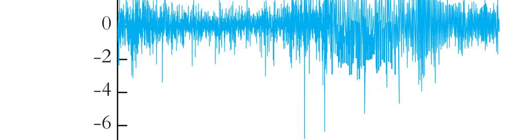
58 What is a trend, ctd. The three series: log Japan GDP clearly has a long-run trend not a straight line, but a slowly decreasing trend fast growth during the 1960s and 1970s, slower during the 1980s, stagnating during the 1990s/2000s. Inflation has long-term swings, periods in which it is persistently high for many years (70s /early 80s) and periods in which it is persistently low. Maybe it has a trend hard to tell. NYSE daily changes has no apparent trend. There are periods of persistently high volatility but this isn t a trend

59 Deterministic and stochastic trends A trend is a long-term movement or tendency in the data. A deterministic trend is a nonrandom function of time (e.g. y t = t, or y t = t 2 ). A stochastic trend is random and varies over time An important example of a stochastic trend is a random walk: Y t = Y t 1 + u t, where u t is serially uncorrelated If Y t follows a random walk, then the value of Y tomorrow is the value of Y today, plus an unpredictable disturbance

60 Deterministic and stochastic trends, ctd. Two key features of a random walk: (i) Y T+h T = Y T Your best prediction of the value of Y in the future is the value of Y today To a first approximation, log stock prices follow a random walk (more precisely, stock returns are unpredictable (ii) var(y T+h T Y T ) = 2 hσ u The variance of your forecast error increases linearly in the horizon. The more distant your forecast, the greater the forecast uncertainty. (Technically this is the sense in which the series is nonstationary ) 14-60

61 Deterministic and stochastic trends, ctd. A random walk with drift is Y t = β 0 +Y t 1 + u t, where u t is serially uncorrelated The drift is β 0 : If β 0 0, then Y t follows a random walk around a linear trend. You can see this by considering the h- step ahead forecast: Y T+h T = β 0 h + Y T The random walk model (with or without drift) is a good description of stochastic trends in many economic time series

62 Deterministic and stochastic trends, ctd. Where we are headed is the following practical advice: If Y t has a random walk trend, then Y t is stationary and regression analysis should be undertaken using Y t instead of Y t. Upcoming specifics that lead to this advice: Relation between the random walk model and AR(1), AR(2), AR(p) ( unit autoregressive root ) A regression test for detecting a random walk trend arises naturally from this development 14-62

63 Stochastic trends and unit autoregressive roots Random walk (with drift): Y t = β 0 + Y t 1 + u t AR(1): Y t = β 0 + β 1 Y t 1 + u t The random walk is an AR(1) with β 1 = 1. The special case of β 1 = 1 is called a unit root*. When β 1 = 1, the AR(1) model becomes Y t = β 0 + u t *This terminology comes from considering the equation 1 β 1 z = 0 the root of this equation is z = 1/β 1, which equals one (unity) if β 1 =

64 Unit roots in an AR(2) AR(2): Y t = β 0 + β 1 Y t 1 + β 2 Y t 2 + u t Use the rearrange the regression trick from Ch 7.3: Y t = β 0 + β 1 Y t 1 + β 2 Y t 2 + u t = β 0 + (β 1 +β 2 )Y t 1 β 2 Y t 1 + β 2 Y t 2 + u t = β 0 + (β 1 +β 2 )Y t 1 β 2 (Y t 1 Y t 2 ) + u t Subtract Y t 1 from both sides: Y t Y t 1 = β 0 + (β 1 +β 2 1)Y t 1 β 2 (Y t 1 Y t 2 ) + u t or Y t = β 0 + δy t 1 + γ 1 Y t 1 + u t, where δ = β 1 + β 2 1 and γ 1 = β

65 Unit roots in an AR(2), ctd. Thus the AR(2) model can be rearranged as, Y t = β 0 + δy t 1 + γ 1 Y t 1 + u t where δ = β 1 + β 2 1 and γ 1 = β 2. Claim: if 1 β 1 z β 2 z 2 = 0 has a unit root, then β 1 + β 2 = 1 (you can show this yourself!) Thus, if there is a unit root, then δ = 0 and the AR(2) model becomes, Y t = β 0 + γ 1 Y t 1 + u t If an AR(2) model has a unit root, then it can be written as an AR(1) in first differences

66 Unit roots in the AR(p) model AR(p): Y t = β 0 + β 1 Y t 1 + β 2 Y t β p Y t p + u t This regression can be rearranged as, Y t = β 0 + δy t 1 + γ 1 Y t 1 + γ 2 Y t γ p 1 Y t p+1 + u t where δ = β 1 + β β p 1 γ 1 = (β β p ) γ 2 = (β β p ) γ p 1 = β p 14-66

67 Unit roots in the AR(p) model, ctd. The AR(p) model can be written as, Y t = β 0 + δy t 1 + γ 1 Y t 1 + γ 2 Y t γ p 1 Y t p+1 + u t where δ = β 1 + β β p 1. Claim: If there is a unit root in the AR(p) model, then δ = 0 and the AR(p) model becomes an AR(p 1) model in first differences: Y t = β 0 + γ 1 Y t 1 + γ 2 Y t γ p 1 Y t p+1 + u t 14-67

68 2. What problems are caused by trends? There are three main problems with stochastic trends: 1. AR coefficients can be badly biased towards zero. This means that if you estimate an AR and make forecasts, if there is a unit root then your forecasts can be poor (AR coefficients biased towards zero) 2. Some t-statistics don t have a standard normal distribution, even in large samples (more on this later) 3. If Y and X both have random walk trends then they can look related even if they are not you can get spurious regressions. Here is an example 14-68

69 Log Japan gdp (smooth line) and US inflation (both rescaled), lgdpjs infs q1 1970q1 1975q1 1980q1 1985q1 time 14-69

70 Log Japan gdp (smooth line) and US inflation (both rescaled), lgdpjs infs q1 1985q1 1990q1 1995q1 2000q1 time 14-70

71 3. How do you detect trends? 1. Plot the data (think of the three examples we started with). 2. There is a regression-based test for a random walk the Dickey-Fuller test for a unit root. The Dickey-Fuller test in an AR(1) or Y t = β 0 + β 1 Y t 1 + u t Y t = β 0 + δy t 1 + u t H 0 : δ = 0 (that is, β 1 = 1) v. H 1 : δ < 0 (note: this is 1-sided: δ < 0 means that Y t is stationary) 14-71

72 DF test in AR(1), ctd. Y t = β 0 + δy t 1 + u t H 0 : δ = 0 (that is, β 1 = 1) v. H 1 : δ < 0 Test: compute the t-statistic testing δ = 0 Under H 0, this t statistic does not have a normal distribution!! You need to compare the t-statistic to the table of Dickey- Fuller critical values. There are two cases: (a) Y t = β 0 + δy t 1 + u t (intercept only) (b) Y t = β 0 + µt + δy t 1 + u t (intercept & time trend) The two cases have different critical values! 14-72

73 Table of DF critical values (a) Y t = β 0 + δy t 1 + u t (intercept only) (b) Y t = β 0 + µt + δy t 1 + u t (intercept and time trend) Reject if the DF t-statistic (the t-statistic testing δ = 0) is less than the specified critical value. This is a 1-sided test of the null hypothesis of a unit root (random walk trend) vs. the alternative that the autoregression is stationary

74 The Dickey-Fuller test in an AR(p) In an AR(p), the DF test is based on the rewritten model, Y t = β 0 + δy t 1 + γ 1 Y t 1 + γ 2 Y t γ p 1 Y t p+1 + u t (*) where δ = β 1 + β β p 1. If there is a unit root (random walk trend), δ = 0; if the AR is stationary, δ < 1. The DF test in an AR(p) (intercept only): 1. Estimate (*), obtain the t-statistic testing δ = 0 2. Reject the null hypothesis of a unit root if the t-statistic is less than the DF critical value in Table 14.5 Modification for time trend: include t as a regressor in (*) 14-74

75 When should you include a time trend in the DF test? The decision to use the intercept-only DF test or the intercept & trend DF test depends on what the alternative is and what the data look like. In the intercept-only specification, the alternative is that Y is stationary around a constant In the intercept & trend specification, the alternative is that Y is stationary around a linear time trend

76 Example: Does U.S. inflation have a unit root? The alternative is that inflation is stationary around a constant 14-76

77 Example: Does U.S. inflation have a unit root? ctd DF test for a unit root in U.S. inflation using p = 4 lags. reg dinf L.inf L(1/4).dinf if tin(1962q1,2004q4); Source SS df MS Number of obs = F( 5, 166) = Model Prob > F = Residual R-squared = Adj R-squared = Total Root MSE = dinf Coef. Std. Err. t P> t [95% Conf. Interval] inf L dinf L L L L _cons DF t-statstic = 2.69 Don t compare this to use the Dickey-Fuller table! 14-77

78 DF t-statstic = 2.69 (intercept-only): t = 2.69 rejects a unit root at 10% level but not the 5% level Some evidence of a unit root not clear cut. This is a topic of debate what does it mean for inflation to have a unit root? We model inflation as having a unit root. Note: you can choose the lag length in the DF regression by BIC or AIC (for inflation, both reject at 10%, not 5% level) 14-78

79 4. How to address and mitigate problems raised by trends If Y t has a unit root (has a random walk stochastic trend), the easiest way to avoid the problems this poses is to model Y t in first differences. In the AR case, this means specifying the AR using first differences of Y t ( Y t ) This is what we did in our initial treatment of inflation the reason was that inspection of the plot of inflation, plus the DF test results, suggest that inflation plausibly has a unit root so we estimated the ARs using Inf t 14-79

80 Summary: detecting and addressing stochastic trends 1. The random walk model is the workhorse model for trends in economic time series data 2. To determine whether Y t has a stochastic trend, first plot Y t, then if a trend looks plausible, compute the DF test (decide which version, intercept or intercept+trend) 3. If the DF test fails to reject, conclude that Y t has a unit root (random walk stochastic trend) 4. If Y t has a unit root, use Y t for regression analysis and forecasting

81 Nonstationarity II: Breaks and Model Stability The second type of nonstationarity we consider is that the coefficients of the model might not be constant over the full sample. Clearly, it is a problem for forecasting if the model describing the historical data differs from the current model you want the current model for your forecasts! (This is an issue of external validity.) So we will: Discuss econometric test procedure for detecting a break Work through an example: the U.S. Phillips curve 14-81

82 A. Tests for a break (change) in regression coefficients Case I: The break date is known Suppose the break is known to have occurred at date τ. Stability of the coefficients can be tested by estimating a fully interacted regression model. In the ADL(1,1) case: Y t = β 0 + β 1 Y t 1 + δ 1 X t 1 + γ 0 D t (τ) + γ 1 [D t (τ) Y t 1 ] + γ 2 [D t (τ) X t 1 ] + u t where D t (τ) = 1 if t τ, and = 0 otherwise. If γ 0 = γ 1 = γ 2 = 0, then the coefficients are constant over the full sample. If at least one of γ 0, γ 1, or γ 2 are nonzero, the regression function changes at date τ

83 Y t = β 0 + β 1 Y t 1 + δ 1 X t 1 + γ 0 D t (τ) + γ 1 [D t (τ) Y t 1 ] + γ 2 [D t (τ) X t 1 ] + u t where D t (τ) = 1 if t τ, and = 0 otherwise The Chow test statistic for a break at date τ is the (heteroskedasticity-robust) F-statistic that tests: H 0 : γ 0 = γ 1 = γ 2 = 0 vs. H 1 : at least one of γ 0, γ 1, or γ 2 are nonzero Note that you can apply this to a subset of the coefficients, e.g. only the coefficient on X t 1. Often, however, you don t have a candidate break date 14-83

84 Case II: The break date is unknown Why consider this case? You might suspect there is a break, but not know when You might want to test for stationarity (coefficient stability) against a general alternative that there has been a break sometime. Often, even if you think you know the break date, that knowledge is based on prior inspection of the series so that in effect you estimated the break date. This invalidates the Chow test critical values (why?) 14-84

85 The Quandt Likelihod Ratio (QLR) Statistic (also called the sup-wald statistic) The QLR statistic = the maximal Chow statistics Let F(τ) = the Chow test statistic testing the hypothesis of no break at date τ. The QLR test statistic is the maximum of all the Chow F- statistics, over a range of τ, τ 0 τ τ 1 : QLR = max[f(τ 0 ), F(τ 0 +1),, F(τ 1 1), F(τ 1 )] A conventional choice for τ 0 and τ 1 are the inner 70% of the sample (exclude the first and last 15%. Should you use the usual F q, critical values? 14-85

86 The QLR test, ctd. QLR = max[f(τ 0 ), F(τ 0 +1),, F(τ 1 1), F(τ 1 )] The large-sample null distribution of F(τ) for a given (fixed, not estimated) τ is F q, But if you get to compute two Chow tests and choose the biggest one, the critical value must be larger than the critical value for a single Chow test. If you compute very many Chow test statistics for example, all dates in the central 70% of the sample the critical value must be larger still! 14-86

87 Get this: in large samples, QLR has the distribution, max a s 1 a q 2 1 Bi ( s) q i= 1 s(1 s), where {B i }, i =1,,n, are independent continuous-time Brownian Bridges on 0 s 1 (a Brownian Bridge is a Brownian motion deviated from its mean), and where a =.15 (exclude first and last 15% of the sample) Critical values are tabulated in SW Table

88 Note that these critical values are larger than the F q, critical values for example, F 1, 5% critical value is

89 Has the postwar U.S. Phillips Curve been stable? Recall the ADL(4,4) model of Inf t and Unemp t the empirical backwards-looking Phillips curve, estimated over ( ): Inf t = Inf t 1.37 Inf t Inf t 3.04 Inf t 4 (.44) (.08) (.09) (.08) (.08) 2.64Unem t Unem t Unem t Unemp t 4 (.46) (.86) (.89) (.45) Has this model been stable over the full period ? 14-89

90 QLR tests of the stability of the U.S. Phillips curve. dependent variable: Inf t regressors: intercept, Inf t 1,, Inf t 4, Unemp t 1,, Unemp t 4 test for constancy of intercept only (other coefficients are assumed constant): QLR = (q = 1). o 10% critical value = 7.12 don t reject at 10% level test for constancy of intercept and coefficients on Unemp t,, Unemp t 3 (coefficients on Inf t 1,, Inf t 4 are constant): QLR = (q = 5) o 1% critical value = 4.53 reject at 1% level o Break date estimate: maximal F occurs in 1981:IV Conclude that there is a break in the inflation unemployment relation, with estimated date of 1981:IV 14-90

91 14-91