Lecture Notes. Applied Mathematics for Business, Economics, and the Social Sciences (4th Edition); by Frank S. Budnick

Transcription

1 1 Lecture Notes Applied Mathematics for Business, Economics, and the Social Sciences (4th Edition); by Frank S. Budnick

2 2 Chapter 2: Linear Equations Definition: Linear equations are first degree equations. Each variable in the equation is raised to the first power. Definition: A linear equation involving two variables x and y has the standard form ax + by= c where a, b and c are constants and a and b cannot both equal zero. Note: The presence of terms having power other than 1 or product of variables, e.g. (xy) would exclude an equation from being linear. Name of the variables may be different from x and y. Examples: 1. 3x + 4y = 7 is linear equation, where a = 3, b = 4, c = 7 2. x = 5 + y is non-liner equation as power of x is not 1. Solution set of an equation Given a linear equation ax + by= c, the solution set for the equation (2.1) is the set of all ordered pairs (x, y) which satisfy the equation. S = {(x, y) ax + by = c} For any linear equation, S consists of an infinite number of elements. Method 1. Assume a value of one variable

3 3 2. Substitute this into the equation 3. Solve for the other variable Example Given 2x + 4y = 16, determine the pair of values which satisfy the equation when x=-2 Solution: Put x=-2 in given equation gives us 4y=16-4, i.e y=3. So the pair (-2,3) is a pair of values satisfying the given equation. Linear equation with n variables Definition A linear equation involving n variables x 1, x 2,..., x n has the general form a 1 x 1 + a 2 x a n x n = b where a, a,, a are non-zero. Definition: The solution set S of a linear equation with n variables as defined above is the collection of n-tuples (x, x,, x ) such that S = {(x,, x ) a x + + a x = b}. As in the case of two variables, there are infinitely many values in the solution set. Example Given an equation 4x 2x + 6x = 0, what values satisfy the equation when x = 2 and x = 1.

4 4 Solution: Put the given values of x and x in the above equation gives x = 7. Thus (2,7,1) is a solution of the above equation. Graphing two variable equations A linear equation involving two variables graphs as a straight line in two dimensions. Method: 1. Set one variable equal to zero 2. Solve for the value of other variable 3. Set second variable equal to zero 4. Solve for the value of first variable 5. The ordered pairs (0, y) and (x, 0) lie on the line 6. Connect these points and extend the line in both directions. Example Graph the linear equation 2x + 4y = 16 Solution: In lectures x-intercept The x-intercept of an equation is the point where the graph of the equation crosses the x-axis, i.e. y=0. y-intercept The y-intercept of an equation is the point where the graph of the equation crosses the y-axis, i.e. x=0 Note: Equations of the form x=k has no y-intercept and equations of the form y=k has no x-intercept

5 5 Slope Any straight line with the exception of vertical lines can be characterized by its slope. Slope represents the inclination of a line or equivalently it shows the rate at which the line raises and fall or how steep the line is. Explanation: The slope of a line may be positive, negative, zero or undefined. The line with slope 1. Positive then the line rises from left to right 2. Negative then the line falls from left to right 3. Zero then the line is horizontal line 4. Undefined if the line is vertical line Note: The sign of the slope represents whether the line falling or raising. Its magnitude shows the steepness of the line. Two point formula (slope) Given any two point which lie on a (non-vertical) straight line, the slope can be computed as the ratio of change in the value of y to the change in the value of x. Slope = = Δy = change in the value of y Δx = change in the vale of x Two point formula (mathematically) The slope m of a straight line connecting two points (x 1, y 1 ) and (x 2, y 2 ) is given by the formula

6 6 Example Slope= Compute the slope of the line segment connecting the two points ( 2, 3) and (1, 9). Solution: Here we have (x, y ) = ( 2,3) and (x, y ) = (1, 9) so using the above formula we get Slope= ( ) = 4 Note: Along any straight line the slope is constant. The line connecting any two points will have the same slope. Slope Intercept form Consider the general form of two variable equation as ax + by = c We can write it as y = a b x + c a The above equation is called the slope-intercept form. Generally, it is written as: y = mx + k m = slope, k = y-intercept Example Rewrite the equation x + 2y = 3x y 4 and find the slope and y -intercept.

7 7 Solution: Rewriting the above we get y = x + 0. Thus slope is and y-intercept is zero. Determining the equation of a straight line Slope and Intercept This is the easiest situation to find an equation of line, if slope of a line is -5 and y-intercept is (0, 15) then we have m= -5, k = 15. We can write down y = 5x + 15 as an equation of line, i.e. 5x + y = 15. Slope and one point If we are given the slope of a line and some point that lies on the line, we can substitute the know slope m and coordinates of the given point into y = mx + k and solve for k. Given a non-vertical straight line with slope m and containing the point (x 1, y 1 ), the slope of the line connecting (x 1, y 1 ) with any other point (x, y) is given by m = y y x x Rearranging gives: y y = m(x x ) Example

8 8 Find the equation of line having slope m = 2 and passing through the point (2, 8). Solution: Here (x, y ) = (2,8) and m = 2, so putting the values in the above equation yields y 8 = 2(x 2) 2x + y = 12. Parallel and perpendicular lines Two lines are parallel if they have the same slope, i.e. m = m. Two lines are perpendicular if their slopes are equal to the negative reciprocal of each other, i.e. m m = 1. Example Find an equation of line through the point (2, 4) and parallel to the line 8x 4y = 20. Solution: From the given equation we have y = 2x 5. Let m = 2 is the slope of the line. Then slope of the required line is same, i.e. m = 2. Thus required equation of line is y ( 4) = 2(x 2) 2x y = 8.

9 9 Lecture 2,3 Chapter 3:Systems of Linear Equations Definition A System of Equations is a set consisting of more than one equation. Dimension: One way to characterize a system of equations is by its dimensions. If system of equations has m equations and n variables, then the system is called an m by n system. In other words, it has m n dimensions. In solving systems of equations, we are interested in identifying values of the variables that satisfy all equations in the system simultaneously. Definition The solution set for a system of linear equations may be a Null set, a finite set or an infinite set. Methods to find the solutions set 1. Graphical analysis method 2. Elimination method 3. Gaussian elimination method Graphical Analysis (2 x 2 system) We discuss three possible outcomes of the solution of 2 x 2 system. 1. Unique solution: We draw the two lines and If two lines intersect at only one point, say (x, y ), then the coordinates of intersection point (x, y ), represent the solution for the system of equations. The system is said to have a unique solution.

10 10 2. No solution: If two lines are parallel (recall that parallel lines have same slope but different y-intercept) then such a system has no solution. The equations in such a system are called inconsistent. 3. Infinitely many solutions: If both equations graph on the same line, an infinite number of points are common in two lines. Such a system is said to have infinitely many solutions. Graphical analysis by slope-intercept relationships Given a (2 2) system of linear equations (in slope-intercept form) y = m x + k y = m x + k where m and m represent the two slopes and k and k denote the two y-intercepts then it has I. Unique solution if m m. II. No Solution if m = m but k k. III. Infinitely many solutions if m = m and k = k. Graphical solutions Limitations: I. Good for two variable system of equations II. Not good for non-integer values III. Algebraic solution is preferred The Elimination Procedure (2 x 2 system)

11 11 Given a (2 2) system of equations I. Eliminate one of the variable by multiplying or adding the two equations II. III. Solve the remaining equation in terms of remaining variable Substitute back into one of the given equation to find the value of the eliminated variable Example Solve the system of equations 2x + 4y = 20 3x + y = 10 Solution: Page 90 in Book or in Lectures Example Solve the system of equations 3x 2y = 6 15x + 10y = 30 Solution: Page 91 in Book/in Lectures Gaussian Elimination Method This method can be used to solve systems of any size. The method begins with the original system of equations. Using row operations, it transforms the original system into an equivalent system from which the solution may be obtained easily. Recall that an equivalent system is one which has the same solution as the original system. In contrast to the Elimination procedure, the transformed system maintain m n dimension Basic Row Operations 1. Both sides of an equation may be multiplied by a nonzero constant. 2. Equations or non-zero multiples of equations may be added or

12 12 subtracted to another equation. 3. The order of equations may be interchanged. Example Determine the solution set for the given system of equations, using Gaussian elimination method. 3x 2y = 7 2x + 4y = 10 Solution: In Lectures (m 2) systems, m >2 When there are more than two equations involving only two variables then 1. We solve two equations first to get a point (x, y) 2. Put the values in the rest of the equations 3. If all equations are satisfied then system has unique solution (x, y). 4. If we get no solution at (1) then system has no solution. 5. If there are infinitely many solutions at step (1), then we select two different equations and repeat (1). Example Determine the solution set for the given (4 2) system of equations, x + 2y = 8 2x 3y = 5 5x + 6y = 8 x + y = 7 Solution: In Lectures or on Page 94 in reference book. Gaussian elimination procedure for 3 x 3 system

13 13 The procedure of Gaussian elimination method for the 3 x 3 system is same as for 2 x 2 system. First we will form coefficient transformation for 3 x 3 system, then convert it to transformed system. Example1 Determine the solution set for the following system of equations 5x 4x + 6x = 24 3x 3x + x = 54 2x + x 5x = 30 Solution: The coefficient matrix of the above system is [ ] Applying the row operations 3 5, 2 + 5, the following form of the above system. +, we get [ ] As one whole row is equal to zero, hence the system of equations has infinitely many solutions. Example2 Determine the solution set for the following system of equations x x + x = 5 3x + x x = 25 2x + x + 3x = 20 Solution: The coefficient matrix of the above system is [ ]

14 14 Applying the row operations 3,, 2,, 3, 4,,, we get the following form of the above system, [ ] Thus we have a unique solution x = 5, x = 10, x = 0. Example3 Determine the solution set for the following system of equations 2x + x + 3x = 10 10x 5x 15x = 30 x + x 3x = 25 Solution: The coefficient matrix of the above system is [ ] Applying the row operations 5 +, + 2,,,, we get the following form of the above system [ ] From row 2 we get 0 = 60, hence the above system of linear equations has no solution. Application

15 15 Product mix problem: A variety of applications are concerned with determining the quantitates of different products which satisfy specific requirements Example A company produces three products. Each needs to be processed through 3 different departments, with following data. Department Products Hours available/week A B C Determine whether there are any combination of three products which would exhaust the weekly capacities of the three departments? Solution: Let x, x, x be the number of units produced per week of product 1, 2 and 3. The conditions to be specified are expressed by the following system of equations. 2x + 3.5x + 3x = 1200 (Department A) 3x + 2.5x + 2x = 1150 (Department B) 4x + 3x + 2x = 1400 (Department C)

16 Now solving the above system by Gaussian elimination method we will get x = 200, x = 100 and x =

17 17 Lecture 04,05 Chapter 4: Mathematical Functions Definition: A function is a mathematical rule that assigns to each input value one and only one output value. Definition: The domain of a function is the set consisting of all possible input values. Definition: The range of a function is the set of all possible output values. Notation The assigning of output values to corresponding input values is often called as mapping. The notation f(x) = y represents the mapping of the set of input values of x into the set of output values y, using the mapping rule f. The equation y = f(x) denotes a functional relationship between the variables x and y. Here x means the input variable and y means the output variable, i.e. the value of y depends upon and uniquely determined by the values of x. The input variable is called the independent variable and the output variable is called the dependent variable. Some examples 1. The fare of taxi depends upon the distance and the day of the week. 2. The fee structure depends upon the program and the type of education (on campus/off campus) you are admitting in.

18 18 3. The house prices depend on the location of the house. Note: The variable x is not always the independent variable, y is not always the dependent variable and f is not always the rule relating x and y. Once the notation of function is clear then, from the given notation, we can easily identify the input variable, output variable and the rule relating them, for example u = g(v) has input variable v, output variable u and g is the rule relating u and v. Example (Weekly Salary Function) A person gets a job as a salesperson and his salary depends upon the number of units he sells each week. Then, dependency of weekly salary on the units sold per week can be represented as y = f(x), where f is the name of the salary function. Suppose your employer has given you the following equation for determining your weekly salary: y = 100 x Given any value of x will result in the value of y with respect to the function f. If x = 5, then y = We write this as, y = f(5) = Example Given the functional relationship f(x) = 5x 10, Find f(0), f( 2) and f(a + b). Solution: As f(x) = 5x 10, so f(0) = 5(0) 10 = 10 f( 2) = 5( 2) 10 = 20 f(a + b) = 5a + 5b 10.

19 19 Domain and Range Recall that the set of all possible input values is called the domain of a function. Domain consists of all real values of the independent variable for which the dependent variable is defined and real. Example Determine the domain of the function f(x) = 2. Solution: f(x) is undefined at 4 x = 0, which gives that give function is not defined at x = ±2. Thus Domain(f) = {x x a an x ±2} Restricted domain and range Up to now we have solved mathematically to find the domains of some types of functions. But for some real world problems, there may be more restriction on the domain e.g. in the weekly salary equation: y = 100 x Clearly, the number of units sold per week can not be negative. Also, they can not be in fractions, so the domain in this case will be all positive natural numbers {1,2,3, }. Further, the employer can also put the condition on the maximum number of units sold per week. In this case, the domain will be defined as: D = {1,2,, u} where u is the maximum number of units sold. Multivariate Functions For many mathematical functions, the value of the dependent variable depends upon more than one independent variable.

20 20 Definition: A functions which contain more than one independent variable are called multivariate function. Definition: A function having two independent variables is called bivariate function. They are denoted by z = f(x, y), where x and y are the independent variables and z is the dependent variable e.g. z = 2x + 5y. In general the notation for a function f where the value of dependent variable depends on the values of n independent variables is z = f(x,, x ). For example, z = 2x + 5x + 4x 4x + x. Types of Functions Constant Functions A constant function has the general form y = f(x) = a Here, domain is the set of all real numbers and range is the single value a, e.g. f(x) = 20. Linear Functions A linear function has the general (slope-intercept) form y = f(x) = a x + a where a is slope and a is y-intercept. For example y = 2x + 3 is represented by a straight line with slope 2 and y-intercept 3.

21 21 The weekly salary function is also an example of linear function. Quadratic Function A quadratic function has the general form y = f(x) = a x + a x + a provided that a 0, e.g. y = 2x + 3. Cubic Function A cubic function has the general form y = f(x) = a x + a x + a x + a provided that a 0, e.g. y = f(x) = x 50x + 10x 1. Polynomial Functions A polynomial function of degree n has the general form y = f(x) = a x + + a x + a Where a,, a and a are real constants such that a 0. All the previous types of functions are polynomial functions. Rational Functions A rational function has the general form y = f(x) = g(x) (x) Where g(x) and (x) are both polynomial functions, e.g.

22 22 y = f(x) = 2x 5x 2x + 3. Composite functions A composite function exists when one function can be viewed as a function of the values of another function. If y = g(u) and u = (x) then composite function y = f(x) = g( (x)). Here x must be in the domain of and (x) must be in the domain of g. For example, if y = g(u) = 3u + 4u and u = (x) = x + 8, then g( ( 2)) = 132. Graphical Representation of Functions The function of one or two variables (independent) can be represented graphically. The functions of one independent variable are graphed in two dimensions, 2-space. The functions in two independent variables are graphed in three dimension, 3- space. Method of graphing 1) To graph a mathematical function, one can simply assign different values from the domain of the independent variable and compute the values of dependent variable. 2) Locate the resulting order pairs on the co-ordinate axes, the vertical axis (y-axis) is used to denote the dependent variable and the horizontal axis (x-axis) is used to denote the independent variable. 3) Connect all the points approximately. Vertical Line Test By definition of a function, to each element in the domain there

23 should correspond only one element in the range. This allows a simple graphical check to determine whether a graph represents a function or not. If a vertical line is drawn through any value in the domain, it will intersect the graph of the function at one point only. If the vertical line intersects at more than one point then, the graph depicts a relation and not a function. 23

24 24 Lecture 05,06 Chapter 5:Linear functions, Applications Recall that a linear function f involving one independent variable x and a dependent variable y has the general form y = f(x) = a x + a, where a 0 and a are constants. Example Consider the weekly salary function y = f(x) = 300x where y is defined as the weekly salary and x is the number of units sold per week. Clearly, this is a weekly function in one independent variable x represents the base salary, i.e. when no units are sold per week and 300 is the commission of each unit sold. 2. The change in weekly salary is directly proportional to the change in the no. of units sold. 3. Slope of 3 indicates the increase in weekly salary associated with each additional unit sold. In general, a linear function having the form y = f(x) = a x + a a change in the value of y is directly proportional to a change in the variable x. Linear function in two independent variables A linear function f involving two independent variables x and x_2 and a dependent variable y has the general form y = f(x, x ) = a x + a x + a where a and a are non-zero constants and a is any constant. 1. This equation tells us that the variable y depends jointly on the values of x and x.

25 25 2. The value of y is directly proportional to the changes in the values of x and x. Example Assume that a salesperson salary depends on the number of units sold of each of two products, i.e. the salary function is given as y = 300x x where y = weekly salary, x is number of units sold of product 1 and x is number of units sold of product 2. This salary function gives a base salary of 2500, commission of 300 on each unit sold of product 1 and 500 on each unit sold of product 2. Linear cost function The organizations are concerned with the costs as they reflect the money flowing out of the organisation. The total cost usually consists of two components: total variable cost and total fixed cost. These two components determine the total cost of the organisation. Example A firm which produces a single product is interested in determining the functions that expresses annual total cost y as a function of the number of units produced x. Accountants indicate that the fixed expenditure each year are 50,000. They also have estimated that raw material costs for each unit produced are 5.50, labour costs per unit are 1.50 in the assembly department, 0.75 in the finishing room, and 1.25 in the packaging and shipping department. Find the total cost function.

26 26 Solution Total cost function = total variable cost + total fixed cost Total fixed cost = 50,000 Total variable cost = total raw material cost + total labour cost y = f(x) = 5.5 x + (1.5 x x x) + 50,000 = 9x + 50,000. The 9 represents the combined variable cost per unit of $9. That is, for each additional unit produced, total cost will increase by $9. Linear Revenue function Revenue: The money which flows out into an organisation from either selling or providing services is often referred to as revenue. Total Revenue = Price Quantity sold Suppose a firm sells product. Let and x be the price of the product and number of units per product respectively. Then the revenue = x + + x. Linear Profit function Profit: The profit of an organisation is the difference between total revenue and total cost. In equation form if total revenue is denoted by (x) and Total cost is (x), where x is quantity produced and sold, then profit (x) is defined as P(x) = (x) C(x). 1. If total revenue exceeds total cost the profit is positive 2. In such case, profit is referred as net gain or net profit 3. On the other hand the negative profit is referred to as a net loss or net deficit.

27 27 Example A firm sells single product for $65 per unit. Variable costs per unit are $20 for materials and $27.5 for labour. Annual fixed costs are $100,000. Construct the profit function stated in terms of x, which is the number of units produced and sold. How much profit is earned if annual sales are 20,000 units. Solution: Here (x) = 65x and total annual cost is made up for material costs, labour costs, and fixed cost. Thus C(x) = 20x x + 100,000 = 47.5 x + 100,000. P(x) = (x) C(x) = 17.5x 100,000. As x = 20,000, so P(20,000) = 250,000. Straight Line Depreciation When organizations purchase an item, usually cost is allocated for the item over the period the item is used. Example A company purchases a vehicle costing $20,000 having a useful life of 5 years, then accountants might allocate $4,000 per year as a cost of owning the vehicle. The cost allocated to any given period is called depreciation. The value of the truck at the limp of purchase is $20,000 but, after 1 year the price will be $ $4000 = $ and so forth. In this case, depreciation can also be thought of as an amount by which the book value of an asset has decreased over the period of time. Thus, the book value declines as a linear function over time. If V

28 28 equals the book value of an asset and t equals time (in years) measured from the purchase date for the previously mentioned truck, then V = f(t). Linear demand function A demand function is a mathematical relationship expressing the way in which the quantity demanded of an item varies with the price charged for it. The relationship between these two variables, quantity demanded and price per unit, is usually inversely proportional, i.e. a decrease in price results in increase in demand. Most demand functions are nonlinear, but there are situations in which the demand relationship either is, or can be approximated by a linear function. uan y man = = f( c un ) Linear Supply Function A supply function relates market price to the quantities that suppliers are willing to produce or sell. The supply function implicates that what is brought to the market depends upon the price people are willing to pay. In contrast to the demand function, the quantity which suppliers are willing to supply usually varies directly with the market price. The higher the market price, the more a supplier would like to produce and sell. The lower the price, the less a supplier would like to produce and sell. uan y u = = f(ma k c ) Break-Even Models Break-even model is a set of planning tools which can be useful in managing organizations. One significant indication of the

29 29 performance of a company is reflected by how much profit is earned. Break-even analysis focuses upon the profitability of a firm and identifies the level of operation or level of output that would result in a zero profit. The level of operations or output is called the break-even point. The break-even point represents the level of operation at which total revenue equals total cost. Any changes from the level of operations will result in either a profit or a loss. Break-even analysis is mostly used when: 1. Firms are offering new products or services. 2. Evaluating the pros and cons of starting a new business. Assumption Total cost function and total revenue function are linear. Break-even Analysis In break-even analysis the main goal is to determine the breakeven point. The break-even point may be expressed in terms of i. Volume of output (or level of activity) ii. Total sale in dollars iii. Percentage of production capacity e.g. a firm will break-even at 1000 units of output, when total sales equal 2 million dollars or when the firm is operating 60% of its plant capacity. Method of performing break-even analysis 1. Formulate total cost as a function of x, the level of output. 2. Formulate total revenue as a function of x. 3. As break-even conditions exist when total revenue equals total cost, so we set C(x) equals (x) and solve for x. The resulting value of x is the break-even level of output and

30 30 denoted by x. An alternate, to step 3 is to construct the profit function P(x) = (x) C(x), set P(x) equal to zero and solve to find x. Example A Group of engineers is interested in forming a company to produce smoke detectors. They have developed a design and estimated that variable costs per unit, including materials, labor, and marketing costs are $ Fixed costs associated with the formation, operation, management of the company and purchase of the machinery costs $250,000. They estimated that the selling price will be 30 dollars per detector. a) Determine the number of smoke detectors which must be sold in order for the firm to break-even on the venture. b) Preliminary marketing data indicate that the firm can expect to sell approximately 30,000 smoke detectors over the life of the project, if the detectors are sold at $30 per unit. Determine expected profits at this level of output. Solution: a) If x equals the number of smoke detectors produced and sold, the total revenue function (x) = 30x. The total cost function is C(x) = 22.5 x + 250,000. We put (x) = C(x) to get x = units. b) P(x) = (x) C(x) = 7.5 x 250,000. Now at x = 30,000, we have P(30,000) = 25,000. Thus the expected loss is $25,000. Market Equilibrium Given supply and demand functions of a product, market equilibrium exits if there is a price at which the quantity demanded equals the quantity supplied.

31 31 Example Suppose demand and supply functions have been estimated for two competing products. 1 2 = (Demand, Product 1) = (Demand, Product 2) 1 2 = 2 4(Supply, Product 1) = 3 6(Supply, Product 2) Determine the price for which the market equilibrium would exist. Solution: The demand and supply functions are linear. The quantity demanded of a given product depends on the price of the product and also on the price of the competing product and the quantity supplied of a product depends only on the price of that product. Market equilibrium would exist in this two-product market place if prices existed and were offered such that 1 = 1 and 2 = 2, solving we get = 221 and = 260. Putting the values in above equations we get 1 = 1 = 438 and 2 = 2 = 774.

32 32 Lecture 07 Chapter 6: Quadratic and Polynomial Functions We focused on linear and non-linear mathematics and linear mathematics is very useful and convenient. There are many phenomena which do not behave in a linear manner and can not be approximated by using linear functions. We need to introduce nonlinear functions. One of the more common nonlinear function is the quadratic function. Definition: A quadratic function involving the independent variable x and the dependent variable y has the general form y = f(x) = ax + bx + c, where a, b, c are constants and a 0. Graphical Representation All quadratic functions have graphs as curves called parabolas. Consider the function y = x then we have The graph of the function is given in the figure given below.

33 33 Properties of Parabolas a) A parabola which opens upward is said to be concave up. The above parabola is concave up. b) A parabola which opens downward is said to be concave down. c) The point at which a parabola either concaves up or down is called the vertex of the parabola. Note: A quadratic function of the form y = ax + bx + c has the vertex coordinates (, 2 ). As we have discussed earlier, here are the results about concavity. 1. If a > 0; the function will graph as parabola which is concave up. 2. If a < 0; the function will graph as parabola which is concave down. Sketching of Parabola Parabolas can be sketched by using the method of chapter 4. But, there are certain things which can make the sketching relative easy. These include,

34 34 1. Concavity of the parabola 2. Y-intercept, where graph meets y-axis. 3. X-intercept, where graph meets x-axis 4. Vertex How to find intercepts 1) Algebraically, y-intercept is obtained when the value of x is equal to zero in the given function. 2) Algebraically, x-intercept is obtained when the value of y is set equal to zero Methods to find the x-intercept The x-intercept of a quadratic equation is determined by finding the roots of an equation. 1) Finding roots by factorisation: If a quadratic can be factored, it is an easy way to find the roots, e.g. x 3x + 2 = 0 can be written as (x 1)(x 2) = 0, which gives x = 1,2 as its roots.. 2) Finding roots by using the quadratic formula The quadratic formula will always identify the real roots of an equation if any exist. The quadratic formula of an equation which has the general form ax + bx + c will be x = ± 2 Taking the same example we get x = ( 3) ± ( 3) + 4(1)(2) 2.

35 35 x = 3 ± 1 2 So we get x = 1,2 as solutions of the equation. Quadratic functions; Applications Quadratic Revenue Function Suppose that the demand function for the product is q = f( ). Here q is the quantity demanded and is the price in dollars. The total revenue from selling q units of price is stated as the product of and q or = q. Since the demand function is stated in terms of price, total revenue can be stated as a function of price, =. f( ) =.. If we let = , then = Quadratic supply function Example Market surveys of suppliers of a particular product have resulted in the conclusion that the supply function is approximately quadratic in form. Suppliers were asked what quantities they would be willing to supply at different market prices. The results of the survey indicated that at market prices of $25, $30 and $ 40, the quantities which suppliers would be willing to offer to the market were 112.5, 250 and 600 (thousands) units, respectively. Determine the equation of the quadratic supply function? Solution: We determine the solution by substituting the three price-quantity combinations into the general equation

36 36 = a + b + c. The resulting system of equations is 625a + 25b + c = a + 30b + c = a + 40b + c = 600 By solving the above system of equations, we get a = 0.5, b = 0, and c = 200. Thus the quadratic supply function is represented by = f( ) = Quadratic demand function Example A consumer survey was conducted to determine the demand function for the same product as in the previous example discussed for supply function. The researchers asked consumers if they would purchase the product at various prices and from their responses constructed estimates of market demand at various market prices. After sample data points were plotted, it was concluded that the demand relationship was estimated best by a quadratic function. The researchers concluded that the quadratic representation was valid for prices between $5 and $45. Three data points chosen for fitting the curve were (5, 2025), (10, 1600) and (20, 900). Just like last example, substituting these data points into the general equation for a quadratic function and solving the resulting system simultaneously gives the demand function =

37 37 Here is the demand stated in thousands of units and equals the selling price in dollars. Polynomial functions A polynomial function of degree n involving the independent variable x and the dependent variable y has the general form y = a x + + a x + a, where a 0, and a,, a are constants. The degree of a polynomial is the exponent of the highest powered term in the expression. Rational Functions Rational functions are the ratios of two polynomial functions with the general form as: f(x) = g(x) (x) = a x + + a x + a b x + + b x + b. Here is n-th degree polynomial function and is m-th degree polynomial function.

38 38 Lecture 08 Chapter 7:Exponential and Logarithmic Functions Properties of exponents and radicals If a, b are positive numbers and m, n are real numbers then: 1. b. b = b 2. = b, b 0 3. b = b. 4. a. b = (ab) 5. b = b = ( b) 6. b = 1 7. b = Exponential Function Definition: A function of the form b, where b > 0, b 1 and x is any real number is called an exponential function to the base x. e.g. f(x) = 10. Characteristics of function f(x) = b x, b > 1 1. Each function f is defined for all values of x. The domain of f is the set of real numbers. 2. The graph of f is entirely above the x-axis. The range of f is the set of positive real numbers. 3. The y-intercept occurs at (0,1). There is no x-intercept. 4. The value of y approaches but never reaches zero as x

39 39 approaches negative infinity. 5. Function y is an increasing function of x, i.e. for x < x, f(x ) < f(x ). 6. The larger the magnitude of the base b, the greater the rate of increase in y as x increases in value. Characteristics of function f(x) = b x, b < 1 1. Each function f is defined for all values of x. The domain of f is the set of real numbers. 2. The graph of f is entirely above the x-axis. The range of f is the set of positive real numbers. 3. The y-intercept occurs at (0,1). There is no x-intercept. 4. The value of y approaches but never reaches zero as x approaches positive infinity. 5. Function y is a decreasing function of x, i.e. for x < x, f(x ) > f(x ). 6. The smaller the magnitude of the base b, the greater the rate of decrease in y as x increases in value. Base e exponential functions A special class of exponential functions is of the form y = a, where is an irrational number approximately equal to Base exponential functions also called as natural exponential functions and are particularly appropriate in modelling continuous growth and decay process, continuous compounding of interest. 2. Base exponential functions are more widely applied than any other class of functions. The two special exponential functions are of is given by the following figure. and. The graph

40 40 Conversion to base e There are instances where base e exponential functions are preferred to those having another base. Exponential functions having a base other than can be transformed into equivalent base functions. For example, if we take = 3, then we have.. = 3. Thus = 3 = f(x). Any positive number x can be expressed equivalently as some power of the base, or we can find an exponent n such that = x. Applications of exponential functions 1. When a growth process is characterized by a constant per cent increase in value, it is referred as an exponential growth process. 2. Decay processes: When a growth process is characterized by a constant per cent decrease in value, it is referred as an exponential decay process. Exponential functions have particular application to growth processes and decay processes. Growth processes include population growth, appreciation in the value of assets, inflation, growth in the rate at which some resources (like energy) are used. Decay processes include declining value of certain assets such as machinery, decline in the efficiency of machine, decline in

41 41 the rate of incidence of certain diseases with the improvement of medical research and technology. Both process are usually stated in terms of time. Example(population growth process) This function characterized by a constant percentage of increase in the value over time. Such process may be describe by the general function; V = f( ) = V, where V = value of function at time, V =value of function at time = 0, k = percentage rate of growth, = time measured in the appropriate units (hours, days, weeks, years, etc). The population of a country was 100 million in 1990 and is growing at the constant rate of 4 per cent per year. The size of populations is P = f( ) = The projected population for 2015, will be P = f(25) = 100. ( ) = Million. Example(Decay functions: price of a machinery) The general form of the exponential decay function is V = f( ) = V. The resale value V of certain type of industrial equipment has been found to behave according to the function V = f( ) = 100,000. then a) Find original value of the price of equipment. b) its value after 5 years.

42 42 Solution: a) We need to find f at = 0, so f(0) = 100,000 = 100,000. Thus the original price is $100,000. b) After 5 years the value will be. ( f(5) = 100,000 ) = 60,650.

43 43 Lecture 09,10,11 Chapter 8:Mathematics of Finance Definition: The Interest is a fee which is paid for having the use of money. We pay interest on loans for having the use of bank s money. Similarly, the bank pay us interest on money invested in savings accounts because the bank has temporary access to our money. 1. Interest is usually paid in proportion to the principal amount and the period of time over which the money is used. 2. The interest rate specifies the rate at which the interest accumulates. 3. It is typically stated as a percentage of the principal amount per period of time, e.g. 18 % per year, 12 % quarterly or 13.5 % per month. Definition: The amount of money that is lent or invested is called the principal. Simple Interest Definition: Interest that is paid solely on the amount of the principal is called simple interest. Simple interest is usually associated with loans or investments which are short-term in nature, computed as I = P n. I = simple interest P = principal = interest rate per time period n = number of time periods While calculating the interest I, it should be noted that both and n are consistent with each other, i.e. expressed in same duration. Example A credit union has issued a 3 year loan of $ Simple interest

44 44 is charged at the rate of 10% per year. The principal plus interest is to be repaid at the end of the third year. Compute the interest for the 3 year period. What amount will be repaid at the end of the third year? Solution: Here P = 5,000, = 0.1, n = 3. Then by using the above formula, we get the simple interest I = (5,000)(0.1)(3) = 1,500. Compound Interest In compound interest, the interest earned each period is reinvested, i.e. added to the principal for purposes of computing interest for the next period. The amount of interest computed using this procedure is called the compound interest. Example Assume that we have deposited $ 8000 in a credit union which pays interest of 8% per year compounded quarterly. The amount of interest at the end of 1 quarter would be: I = 8000(0.08)(0.25) = 160. Here n=0.25 year, with interest left in the account, the principal on which interest is earned in the second quarter is the original principal plus $160 earned during the first quarter P = P + I = = The interest earned during second quarter is I = 8160(. 25)(. 08) = Continuing this way, after the year the total interest earned would be At the end of one year, the compound amount would be The simple interest after 1 year would be: I = 800(.08)(1) = 640

45 45 The difference between simple and compound interest is = Continuous compounding The continuous compounding can be thought of as occurring infinite number of times. It can be computed by the following formula. Continuous compounding S = P, where = Rate of interest, = Time period, P = Principal. Example Compute the growth in a $ 10,000 investment which earns interest at 10 per cent per year over the period of 10 years. Solution: Here = 0.1, = 10, and P = 10,000. Hence S = (10,000). ( ) = 27,183. Note: The value of an investment increases with increased frequency of compounding. If we compute the interest by using different frequency, we get the following. 1. Simple interest in 10 years will raise the amount to 20, Annual compounding in 10 years will raise the amount to 25, Semi-annual compounding in 10 years will raise the amount to 26, Quarterly compounding in 10 years will raise the amount to 26,830.

46 46 Single-Payment computations Suppose we have invested a sum of money and we wish to know that: what will be the value of money at some time in the future? In knowing this, we assume that any interest is computed on compounding basis. Recall that the amount of money invested is called the principal and the interest earned is called (after some period of time) the compound amount. Given any principal invested at the beginning of a time period, the compound amount at the end of the period is calculated as: S = P + P, where P = principal, = interest rate in per cent, S = compound amount. A period may be any unit of time, e.g. annually, quarterly. Compound amount formula To get a general formula, we let P = principal, = interest rate per compounding period n= number of compounding periods (number of periods in which the principal has earned interest) S= compound amount after 1 period= S = P(1 + ). Compound amount after 2 periods = P(1 + ) + P(1 + ) = P(1 + ) Similarly, compound amount after 3 periods = P(1 + ). Thus after n periods the compound amount S = P(1 + ). Note: The compound amount S is an exponential function of the number of compounding periods n, so S = f(n). Definition: The expression (1 + ) is called a compound

47 47 amount factor. Example Suppose that $ 1000 is invested in a saving bank which earns interest at the rate of 8 % per year compounded annually. If all interest is left in the account, what will be the account balance after 10 years? Solution: Using S = P(1 + ), we get S = 1000( ) = Present value computation The compound amount formula S = P(1 + ) is an equation involving four variables,.i.e. S, P,, n. Thus knowing the values of any of the 3 variables, we can easily find the 4 th one. Rewriting the formula as: P = ( ) P denotes the present value of the compound amount. Example A person can invest money in saving account at the rate of 10 % per year compounded quarterly. The person wishes to deposit a lump sum at the beginning of the year and have that sum grow to $ 20,000 over the next 10 years. How much money should be deposited? How much amount of money should be invested at the rate of 10 % per year compounded quarterly, if the compound amount is $ after 10 years? Solution: As P = P = S (1 + ) ( ) =

48 48 Definition: The factor ( ) is called the present value factor. Other applications of compound amount formula 1. The following examples will illustrate the other applications of the compound amount formula, when and n are unknown. 2. When a sum of money is invested, there may be a desire to know that how long it will take for the principal to grow by certain percentage. Example A person wishes to invest $ and wants the investment to grow to $ over the next 10 years. At what annual interest rate the required amount is obtained assuming annual compounding? Solution: Page number 315 in book or in Lectures Effective Interest Rates The stated annual interest rate is usually called nominal rate. We know that when interest is compounded more frequently then interest earned is greater than earned when compounded annually. When compounding is done more frequently than annually, then effective annual interest rates can be determined. Two rates would be considered equivalent if both results in the same compound amount. Let equals the effective annual interest rate, is the nominal annual interest rate and m is the number of compounding periods per year. The equivalence between the two rates suggests that if a principal P is invested for n years, the two compound amounts would be the same, or Solving for, we get P(1 + ) = P (1 + m )

49 49 = (1 + m ) 1. Annuities and their Future value An annuity is a series of periodic payments, e.g. monthly car payment, regular deposits to savings accounts, insurance payments. We assume that an annuity involves a series of equal payments. All payments are made at the end of a compounding period, e.g. a series of payments, each of which equals 1000 at the end of each period, earn full interest in the next period and does not qualify for the interest in the previous period. Example A person plans to deposit $ 1000 in a tax-exempt savings plan at the end of this year and an equal sum at the end of each year following year. If interest is expected to be earned 6 % per year compounded annually, to what sum will the investment grow at the time of the 4 th deposit? Solution: We can determine the value of S by applying the compound amount formula to each deposit, determining its value at the time of the 4-th deposit. These compound amounts may be summed for the four deposits to determine S. First deposit earns interest for 3 years, 4th deposit earns no interest. The interest earned on first 3 deposits is $ Thus S = Formula The procedure used in the above example is not practical when dealing with large number of payments. In general to compute the sum S, we use the following formula.

50 50 S = (1 + ) 1 = S The special symbol S, which is pronounced as S sub n angle i, is frequently used to abbreviate the series compound amount factor ( ). Now we solve the last example by this formula. We have S = 1000 S (. ) = , by using the table III at the page T-10 in book. Example A boy plans to deposit $ 50 in a savings account for the next 6 years. Interest is earned at the rate of 8% per year compounded quarterly. What should her account balance be 6 years from now? How much interest will he earn? Solution: Here = 50, =. = 0.02, n = 6 4 = 24. We need to find S = 50. S (. ) = 50(30.421) = Determining the size of an annuity The formula S = S has four variables. So like compound amount formula, if any three of them are know, we can find the fourth one. For example if the rate of interest is known, what amount should be deposited each period in order to reach some other specific amount? We solve for, As S = S, so we have = S S = S [ 1 S ]

51 51 The expression in brackets is the reciprocal of the series compound amount factor. This factor is called sinking fund factor. Because the series of deposits used to accumulate some future sum of money is often called a sinking fund. The values for the sinking fund factor [ ] can be found in table IV, pages T15-T17 in the book. Example A corporation wants to establish a sinking fund beginning at the end of this year. Annual deposits will be made at the end of this year and for the following 9 years. If deposits earn interest at the rate of 8 % per year compounded annually, how much money must be deposited each year in order to have $ 12 million at the time of the 10 th deposit.? How much interest will be earned? Solution: Here S = 12 m on, = 0.08, n = 10. Thus = S [ 1 S (. ) ] = 12,000, = deposits of $ will be made during this period, total deposits will equal to $ Interest earned = 12 million = $ Example Assume in the last example that the corporation is going to make quarterly deposits and that the interest is earned at the rate of 8 % per year compounded quarterly. How much money should be deposited each quarter? How much less will the company have to deposit over the 10 year period as compared with annual deposits and annual compounding?

52 52 Solution: Here S = 12 m on, =. = 0.02, n = 40. Thus = S [ 1 S (. ) ] = 12,000, = Since there will be 40 deposits of $198720, total deposits over the 10 year period will equal $ Comparing with annual deposits and annual compounding in the last example, total deposit required to accumulate the $12million, will be = less under quarterly compounding. Annuities and their Present value There are applications which relate an annuity to its present value equivalent. e.g. we may be interested in knowing the size of a deposit which will generate a series of payments (an annuity) for college, retirement years, or given that a loan has been made, we may be interested in knowing the series of payments (annuity) necessary to repay the loan with interest. The present value of an annuity is an amount of money today which is equivalent to a series of equal payments in the future. An assumption is that: the final withdrawal would deplete the investment completely. Example A person recently won a state lottery. The terms of the lottery are that the winner will receive annual payments of $ 20,000 at the end of this year and each of the following 3 years. If the winner could invest money today at the rate of 8 % per year compounded annually, what is the present value of the four payments? Solution: If A defines the present value of the annuity, we might determine the value of A by computing the present value of each payment. Here S = 20000, = 0.08 then using P = ( )

53 53 For n = 1 => P = For n = 2 => P = For n = 3 => P = For n = 4 => P = Calculating the sum we get = As with the future value of an annuity, we can find the general formula for the present value of an annuity. In case of large number of payments the method of example is not practical. Formula If = Amount of an annuity = Interest rate per compounding period n = Number of annuity payments = Present value of an annuity then = [ (1 + ) 1 ( + 1) ] = a The above equation is used to compute the present value of an annuity consisting of n equal payments, each made at the end of n periods. Definition: The expression [ ( ) ] is called the series ( ) present worth factor. Its value can be found in table V in book.

54 54 Example Parents of a teenager girl want to deposit a sum of money which will earn interest at the rate of 9 % per year compounded semiannually. The deposit will be used to generate a series of 8 semi annual payments of $2500 beginning 6 months after the deposit. These payments will be used to help finance their daughter s college education. What amount must be deposited to achieve their goal? How much interest will be earned? Solution: Here = 2500, =. = 0.045, n = 8. Thus we find = 2500a (. ) = = Since the $ will generate eight payments totalling $20000, interest earned will be =$ Determining the size of an annuity Given the value of, we can find = size of the corresponding annuity. = = [ 1 ] a a The expression [ ] is called the capital recovery factor. Table VI at page T-22 contain selected values for this factor. Example For example given a loan of $ which is received today, what quarterly payments must be made to repay the loan in 5 years if interest is charged at the rate of 10 % per year, compounded quarterly? How much interest will be paid on the loan? Solution: Here = 10,000, =. = 0.025, n = 20.

55 55 Using the above formula = [ 1 a (. ) ] = = There will be 20 payments totalling $12830, thus interest will be equal to $2830 on the loan.

56 56 Lecture 12,13 Chapter 10 Linear Programming:An Introduction Basic concepts Linear Programming (LP) is a mathematical optimization technique. By optimization we mean a method or procedure which attempts to maximize or minimize some objective, e.g., maximize profit or minimize cost. In any LP problem certain decisions need to be made, these are represented by decision variables x. The basic structure of a LP problem is either to maximize or minimize an objective function while satisfying a set of constraints. 1. Objective function is the mathematical representation of overall goal stated as a function of decision variables x, examples are profit levels, total revenue, total cost, pollution levels, market share etc. 2. The Constraints, also stated in terms of x, are conditions that must be satisfied when determining levels for the decision variables. They can be represented by equations or by inequalities ( and/or types). The term Linear is due to the fact that all functions and constraints in the problem are linear. Example A simple linear programming problem is Maximize z = 4x + 2x Subject to 2x + 2x 24 4x + 3x 30. The objective is to maximize z, which is stated as a linear function of two decision variables x and x. In choosing values for x and x two constraints must be satisfied. The constraints are

57 57 represented by the two linear inequalities. A Scenario (a LP example) A firm manufactures two products, each of which must be processed through two departments 1 and 2. Product A Product B Weekly Labor Capacity Department 1 3 h per unit 2 h per unit 120 h Department 2 4 h per unit 6 h per unit 260 h Profit Margins $5 per unit $6 per unit If x and y are the number of units produced and sold, respectively of product A and B, then the total profit z is z = 5x + 6y The restrictions in deciding the units produced are given by the inequalities: 3x + 2y 120 (Department 1) 4x + 6y 260 (Department 1) We also know that x and y can not be negative. So the LP model which represents the stated problem is: Maximize z = 5x + 6y Subject to 3x + 2y 120 (1) 4y + 6y 260 (2) x 0 (3) y 0 (4) Inequalities (1) and (2) are called structural constraints, while (3) and (4) are non-negativity constraints.

58 58 Notably, the function z is our objective function that needs to be maximized. Graphical Solutions When a LP model is stated in terms of 2 decision variables, it can be solved by graphical methods. Before discussing the graphical solution method, we will discuss the graphics of linear inequalities. Graphics of Linear Inequalities Linear inequalities which involve two variables can be represented graphically in two dimensions by a closed half space of a certain type of the certain plane. The half space consists of the boundary line representing the equality part of the inequality and all points on one side of the boundary line (representing the strict inequality). Graph the boundary which represents the equation. Determine the side that satisfy the strict inequality. System of Linear Inequalities In LP problems we will be dealing with system of linear inequalities. We will be interested to determine the solution set which satisfies all the inequalities in the system of constraints. Region of feasible solution The first step in graphical procedure is to identify the solution set for the system constraints. This solution set is called region of feasible solution. It includes all combinations of decision variables which satisfy the structural and non-negativity constraints. Corner point solution Given a linear objective function in a linear programming problem, the optimal solution will always include a corner point on the region of feasible solution. This will hold, irrespective of the slope of objective function and for either maximization or minimization

59 59 problems. We can use a method, called corner point method, to solve the linear programming problems. The corner point method for solving LP problems is as follows. 1. Graphically identify the region of feasible solutions. 2. Determine the coordinates of each corner point on the region of feasible solution. 3. Substitute the coordinates of the corner points into the objective function z to determine the corresponding value of z. 4. The required solution occur at the corner point yielding, (highest value of z in maximization problems)/ (lowest value of z in minimization problems). Alternative Optimal Solutions There is a possibility of more than one optimal solutions in LP problem. Alternative optimal solution exists if the following two conditions are satisfied. 1. The objective function must be parallel to the constraint which forms an edge or boundary on the feasible region 2. The constraint must form a boundary on the feasible region in the direction of optimal movement of the objective function Example (Page 437 in Book) Use corner-point method to solve: Maximize z = 20x + 15x Subject to 3x + 4x 60 (1) 4x + 3x 60 (2) x 10 (3) x 12 (4) x, x 0 (5) Solution: The figure shows all the corner points of the given LP problem. Corner O(0,0) (0,12) B(10,0) C(4,12) 20 D(10, point Value of z 3 ) E(60 7, 60 7 )

60 60 Optimal Solution occurs at the point D and E. In fact, any point along the line DE will give this optimal solution. Both the conditions for alternative optimal solutions were satisfied in this example. The objective function was parallel to the constraint (2) and the constraint (2) was a boundary line in the direction of the optimal movement of objective function. No Feasible Solutions The system of constraints in an LP problem may have no points which satisfy all constraints. In such cases, there are no points in the solution set and hence the LP problem is said to have no feasible solution. Applications of Linear Programming Diet Mix Model A dietician is planning the menu for the evening meal at a university dining hall. Three main items will be served, all having different nutritional content. The dietician is interested in providing at least the minimum daily requirement of each of three vitamins in this one meal. Following table summarizes the vitamin contents

61 61 per ounce of each type of food, the cost per ounce of each food, and minimum daily requirements (MDR) for the three vitamins. Any combination of the three foods may be selected as long as the total serving size is at least 9 ounces. Vitamins Food Cost per Oz, $ 1 50mg 20mg 10mg mg 10mg 50mg mg 30mg 20mg 0.12 Minimum daily requirement (MDR) 290mg 200mg 210mg The problem is to determine the number of ounces of each food to be included in the meal. The objective is to minimize the cost of each meal subject to satisfying minimum daily requirements of the three vitamins as well as the restriction on minimum serving size. Solution: Let x j equal the number of ounces included of food j. The objective function should represent the total cost of the meal. Stated in dollars, the total cost equals the sum of the costs of the three items, or Z = 0.10x x x 3 The constraint for each vitamin will have the form. Milligrams of vitamin intake MDR Milligrams from food 1 + milligram from food 2+ milligram from food 3 MDR

62 62 The constraints are, respectively, 50x x x (vitamin 1) 20x x x (vitamin 2) 10x x x (vitamin 3) The restriction that the serving size be at least 9 ounces is stated as x 1 + x 2 + x 3 9 (minimum serving size) The complete formulation of the problem is as follows: Minimize z = 0.10x x x 3 subject to 50x x x x x x x x x x 1 + x 2 + x 3 9 x 1, x 2, x 3 0 Transportation Model Transportation models are possibly the most widely used linear programming models. Oil companies commit tremendous resources to the implementation of such models. The classic example of a transportation problem involves the shipment of some homogeneous commodity from m sources of supply, or origins, to n points of demand, or destinations. By homogeneous we mean that there are no significant differences in the quality of the item provided by the different sources of supply. The item characteristics are essentially the same. Example (Highway Maintenance) A medium-size city has two locations in the city at which salt and sand stockpiles are maintained for use during winter icing and

63 63 snowstorms. During a storm, salt and sand are distributed from these two locations to four different city zones. Occasionally additional salt and sand are needed. However, it is usually impossible to get additional supplies during a storm since they are stockpiled at a central location some distance outside the city. City officials hope that there will not be back-to-back storms. The director of public works is interested in determining the minimum cost of allocating salt and sand supplies during a storm. Following table summarizes the cost of supplying 1 ton of salt or sand from each stockpile to each city zone. In addition, stockpile capacities and normal levels of demand for each zone are indicated (in tons) Solution: In formulating the linear programming model for this problem, there are eight decisions to make-how many tons should be shipped from each stockpile to each zone. Let x ij equal the number of tons supplied from stockpile i to zone j. For example, x 11 equals the number of tons supplied by stockpile 1 to zone 1. Similarly, x 23 equals the number of tons supplied by stockpile 2 to zone 3. This double-subscripted variable conveys more information than the variables x 1, x 2,, x 8. Give this definition of the decision variables, the total cost of distributing salt and sand has the form: Total Cost = 2x x x x 14 +4x x x 23 +3x 24 This is the objective function that we wish to minimize. For stockpile 1, the sum of the shipments to all zones cannot exceed 900 tons, or x 11 + x 12 + x 13 + x (stockpile 1) The same constraint for stockpile 2 is

64 64 x 21 + x 22 + x 23 + x (stockpile 2) The final class of constraints should guarantee that each zone receives the quantity demanded. For zone 1, the sum of the shipments from stockpiles 1 and 2 should equal 300 tons, or x 11 + x 21 = 300 (zone 1) The same constraints for the other three zones are, respectively, x 12 + x 22 = 450 (zone 2) x 13 + x 23 = 500 (zone 3) x 14 + x 24 = 350 (zone 4) The complete formulation of the linear programming model is as follows: Minimize z = 2x x x x x x x 23 +3x 24 Subject to x 11 + x 12 + x 13 + x x 21 + x 22 + x 23 + x x 11 + x 21 = 300 x 12 + x 22 = 450 x 13 + x 23 = 500 x 14 + x 24 = 350 x 11, x 12, x 13, x 14, x 11, x 22, x 23, x 24 0

65 65 Lecture 14,15,16,17 Chapter 11:The Simplex and Computer Solution Methods Simplex Preliminaries Graphical solution methods are applicable to LP problems involving two variables. The geometry of three variable problems is very complicated, and beyond three variables, there is no geometric frame of reference, so we need some nongraphic Method. The most popular non-graphical procedure is called The Simplex Method. This is an algebraic procedure for solving system of equations where an objective function needs to be optimized. It is an iterative process, which identifies a feasible starting solution. The procedure then searches to see whether there exists a better solution. Better is measured by whether the value of the objective function can be improved. If better solution is signaled, the search resumes. The generation of each successive solution requires solving a system of linear equations. The search continues until no further improvement is possible in the objective function Requirements of the Simplex Method 1. All constraints must be stated as equations. 2. The right side of the constraint cannot be negative. 3. All variables are restricted to nonnegative values. Most linear programming problems contain constraints which are inequalities. Before we solve by the simplex method, these inequalities must be restated as equations. The transformation

66 66 from inequalities to equations varies, depending on the nature of the constraints. Transformation procedure for constraints For each less than or equal to constraint, a non-negative variable, called a slack variable, is added to the left side of the constraint. Note that the slack variables become additional variables in the problem and must be treated like any other variables. That means they are also subject to Requirement 3 that is, they cannot assume negative values. For example 3x 2x 4 will be transformed as 3x + 2x + S = 4. Transformation procedure for constraints For each greater than or equal to constraint, a non-negative variable E, called a surplus variable, is subtracted from the left side of the constraint. In addition, a non-negative variable A, called an artificial variable, is added to the left of side of the constraint. The artificial variable has no real meaning in the problem; its only function is to provide a convenient starting point (initial guess) for the simplex. For example x + x 10 will be transformed to x + x E + = 10. Transformation procedure for = constraints For each equal to constraint, an artificial variable, is added to the left of side of the constraint. For example 3x + x = 10 will be transformed to 3x + x + = 10. Example Transform the following constraint set into the standard form required by the simplex method x 1 + x 2 100, 2x 1 + 3x 2 40, x 1 x 2 = 25, x 1, x 2 0

67 67 Solution: The transformed constraint set is x 1 + x 2 + S x 1 + 3x 2 E 2 + A 2 40 x 1 x 2 + A 3 = 25 x 1, x 2, S 1, E 2, A 2, A 3 0 Note that each supplemental variable (slack, surplus, artificial) is assigned a subscript which corresponds to the constraint number. Also, the non-negativity restriction (requirement 3) applies to all supplemental variables. Example An LP problem has 5 decision variables; 10 ( ) constraints; 8 ( ) constraints; and 2 (=) constraints. When this problem is restated to comply with requirement 1 of the simplex method, how many variables will there be and of what types? Solution: There will be 33 variables: 5 decision variables, 10 slack variables associated with the 10 ( ) constraints, 8 surplus variables associated with the 8 ( ) constraints, and 10 artificial variables associated with the ( ) and (=) constraints = 33 Basic Feasible Solutions Let s state some definitions which are significant to our coming discussions. Assume the standard form of an LP problem which has m structural constraints and a total of n decision and supplemental variables. Definition: A feasible solution is any set of values for the n variables which satisfies both the structural and non-negativity constraints.

68 68 Definition: A basic solution is any solution obtained by setting (n m) variables equal to 0 and solving the system of equations for the values of the remaining m variables. Definition: The (n m) variables which have been assigned values of 0, are called non-basic variables. The rest of the variables are called basic variables. Definition: A basic feasible solution is a basic solution which also satisfies the non-negativity constraints. Thus optimal solution can be found by performing a search of the basic feasible solution. The Simplex Method Before we begin our discussions of the simplex method, let s provide a generalized statement of an LP model. Given the definitions x j = j-th decision variable c j = coefficient on j-th decision variable in the objective function. a ij = coefficient in the i-th constraint for the j-th variable. b i = right-hand-side constant for the i-th constraint The generalized LP model can be stated as follows: Optimize (maximize or minimize) z = c 1 x 1 + c 2 x c n x n subject to a 11 x 1 + a 12 x a 1n x n (,, =) b1 (1) a 21 x 1 + a 22 x a 2n x n (,, =) b2 (2)... a m1 x 1 + a m2 x a mn x n (,, =)b m (m) x 1 0 x x n 0

69 69 Solution by Enumeration Consider a problem having m ( ) constraints and n variables. Prior to solving by the simplex method, the m constraints would be changed into equations by adding m slack variables. This restatement results in a constraint set consisting of m equations and m + n variables. Example Solve the following LP problem. Maximize z = 5x 1 + 6x 2 subject to 3x 1 + 2x (1) 4x 1 + 6x (2) x 1, x 2 0 Solution: The constraint set must be transformed into the equivalent set. 3x 1 + 2x 2 + S 1 = 120 4x 1 + 6x 2 + S 2 = 260 x 1, x 2, S 1, S 2 0 The constraint set involves two equations and four variables. Of all the possible solutions to the constraint set, an optimal solution occurs when two of the four variables in this problem are set equal to zero and the system is solved for the other two variables. The question is, which two variables should be set equal to 0 (should be non-basic variables)? Let s enumerate the different possibilities. 1. If S 1 and S 2 are set equal to 0, the constraint equations become 3x 1 + 2x 2 = 120 4x 1 + 6x 2 = 260 Solving for the corresponding basic variable x 1 and x 2 results in x 1 = 20 and x 2 = If S 1 and x 1 are set equal to 0, the system becomes 2x 2 = 120

70 70 6x 2 + S 2 = 260 Solving for the corresponding basic variables x 2 and S 2 results in x 2 = 60 and S 2 = 100 Following table summarizes the basic solutions, that is, all the solution possibilities given that two of the four variables are assigned 0 values. Notice that solutions 2 and 5 are not feasible. They each contain a variable which has a negative value, violating the non-negativity restriction. However, solutions 1, 3, 4 and 6 are basic feasible solutions to the linear programming problem and are candidates for the optimal solution. The following figure is the graphical representation of the set of constraints.

71 71 Specifically, solution 1 corresponds to corner point C, solution 3 corresponds to corner point B, solution 4 corresponds to corner point D, and solution 6 corresponds to corner point A. Solution 2 and 5, which are not feasible, correspond to the points E and F shown in the figure. Incorporating the Objective Function In solving by the simplex method, the objective function and constraints are combined to form a system of equations. The objective function is one of the equations, and z becomes an additional variable in the system. In rearranging the variables in the objective function so that they are all on the left side of the equation, the problem is represented by the system of equations. z 5x 1 6x 2 0S 1 OS 2 = 0 (0) 3x 1 + 2x 2 + S 1 = 120 (1) 4x 1 + 6x 2 + S 2 = 260 (2) Note: The objective function is labeled as Eq.(0). The objective is to solve this (3 x 5) system of equations so as to maximize the

72 72 value of z. Since we are particularly concerned about the value of z and will want to know its value for any solution, z will always be a basic variable. The standard practice, however, is not to refer to z as a basic variable. The terms basic variable and non-basic variable are usually reserved for other variables in the problem. Simplex Procedure The simplex operations are performed in a tabular format. The initial table, or tableau, for our problem is shown in the table below. Note that there is one row for each equation and the table contains the coefficients of each variable in the equations and bi column contains right hand sides of the equation. Summary of simplex procedure We summaries the simplex procedure for maximization problems having all ( ) constraints. First, add slack variables to each constraint and the objective function and place the variable coefficients and right-hand-side constants in a simplex tableau: 1- Identify the initial solution by declaring each of the slack variables as basic variables. All other variables are non-basic in the initial solution. 2- Determine whether the current solution is optimal by applying rule 1 [Are all row (0) coefficients 0?]. If it is not optimal, proceed to step 3.

73 73 3- Determine the non-basic variable which should become a basic variable in the next solution by applying rule 2 [most negative row (0) coefficient]. 4- Determine the basic variable which should be replaced in the next solution by applying rule 3 (min b i /a ik ratio where a ik > 0) 5- Applying the Gaussian elimination operations to generate the new solution (or new tableau). Go to step 2. Example(Page 488 in Book) Solve the following linear programming problem using the simplex method. Maximize z = 2x x 2 + 8x 3 subject to 2x 1 + 2x 2 + x x 1 2x 2 + 5x x 1 + 5x 2 + 4x x 1, x 2, x 3 0 Solution: Detailed solution is in Book/Lectures. Maximization Problems with Mixed Constraints For a maximization problem having a mix of (,, and =) constraints the simplex method itself does not change. The only change is in transforming constraints to the standard equation form with appropriate supplemental variables. Recall that for each ( ) constraint, a surplus variable is subtracted and an artificial variable is added to the left side of the constraint. For each (=) constraint, an artificial variable is added to the left side. An additional column is added to the simplex tableau for each supplemental variable. Also, surplus and artificial variables must be assigned appropriate objective function coefficients (c, values) Surplus variables usually re-assigned an objective function coefficient of 0. Artificial variables are assigned objective function coefficient of M, where M is a very large number. This is to make the artificial variables unattractive in the problem.

74 74 In any linear programming problem, the initial set of basic variables will consist of all the slack variables and all the artificial variables which appear in the problem. Example (Page 491 in Book) Maximize z = 8x 1 + 6x 2 subject to 2x 1 + x x 1 + 8x 2 96 x 1, x 2 0 We have a maximization problem which has a mix of a ( ) constraint and a ( ) constraint. Solution: (In Book/ Lectures) Minimization Problems The simplex procedure is slightly different when minimization problems are solved. Aside from assigning artificial variables objective function coefficients of +M, the only difference relates to the interpretation of row (0) coefficients. The following two rules are modifications of rule 1 and rule 2. These apply for minimization problems. Rule 1A: Optimality Check in Minimization Problem. In a minimization problem, the optimal solution has been found if all row (0) coefficients for the variables are less than or equal to 0. If any row (0) coefficients are positive for non-basic variables, a better solution can be found by assigning a positive quantity to these variables. Rule 2A: New basic variable in minimization problem. In a minimization problem, the non-basic variable which will replace a current basic variable is the one having the largest positive row (0) coefficient. Ties may be broken arbitrarily.

75 75 Example (page 493 in Book) Solve the following linear programming problem using the simplex method. Minimize z = 5x 1 + 6x 2 subject to x 1 + x x 1 + 4x 2 24 x 1, x 2 0 Solution: This problem is first rewritten with the constraints expressed as equations, as follows: Minimize z = 5x 1 + 6x 2 + 0E 1 + 0E 2 + MA 1 + MA 2 subject to x 1 + x 2 E 1 + A 1 = 10 2x 1 + 4x 2 E 2 + A 2 = 24 x 1, x 2, E 1, E 2, A 1, A 2 0 Basic Varia bles z x 1 x 2 E 1 E 2 A 1 A 2 Need to Be Transformed to Zero b i Row Number M M 0 (0) A (1) A (2) The initial tableau for this problem appears in above table. Note that the artificial variables are the basic variables in this initial solution. These M coefficient in row (0) must be changed to 0 using row operations if the value of z is to be read from row (0).

76 76 In this initial solution the non-basic variables are x 1, x 2, E 1, and E 2. The basic variables are the two artificial variables with A 1 = 10, A 2 = 24, and z = 34M. Applying rule 1A, we conclude that this solution is not optimal. The x 2 column becomes the new key column. Applying rule 1A, we conclude that this solution is optimal. Therefore, z is minimized at a value of 52 when x 1 = 8 and x 2 = 2. Special Phenomena In Chapter 10, certain phenomena which can arise when solving LP problems were discussed. Specifically, the phenomena of alternative optimal solutions, no feasible solution, and unbounded solutions were presented. In this section we discuss the manner in which these phenomena occur when solving by the simplex method. Alternative Optimal Solutions An Alternative optimal solution results when the objective function is parallel to a constraint which binds in the direction of optimization. In two-variable problems we are made aware of alternative optimal solutions with the corner-point method when a tie occurs for the optimal corner point.

77 77 When using the simplex methods, alternative optimal solutions are indicated when 1- an optimal solution has been identified, 2- the row (0) coefficient for a non-basic variable equals zero. The first condition confirms that there is no better solution than the present solution. The presence of a 0 in row (0) for a nonbasic variable indicates that the non-basic variable can become a basic variable (can become positive) and the current value of the objective function (known to be optimal) will not change. Example (page 491 in Book) Maximum z = 6x 1 + 4x 2 subject to x 1 + x 2 5 3x 1 + 2x 2 12 x1, x2 0 Solution (In Lectures/Book) No Feasible Solutions A problem has no feasible solution if there are no values for the variables which satisfy all the constraints. The condition of no feasible solution is signaled in the simplex method when an artificial variable appears in an optimal basis at a positive value. Let s solve the following LP problem, which, by inspection, has no feasible solution. Example (Page 499 in Book ) Maximize z = 10x x 2 subject to x + x 2 5 x 1 + x 2 20 x 1, x 2 0 Solution: (In Lectures/Book) Unbounded Solutions Unbounded solutions exist when there is an unbounded solution space. Improvement in the objective function occurs with

78 78 movement in the direction of the unbounded portion of the solution space. If at any iteration of the simplex method the a ik values are all 0 or negative for the variable selected to become the new basic variable, there is an unbounded solution for the LP problem. Example (Page 500-Book ) Maximize z = 2x 1 + 3x 2 subject to x x 1 x 2 30 x 1, x 2 0 Solution: (In Lectures/Book) The Dual Problem Every LP problem has a related problem called the dual problem or, simply, the dual. Given an original LP problem, referred to as the primal problem, or primal, the dual can be formulated from information contained in the primal. Given an LP problem, its solution can be determined by solving either the original problem or its dual. Formulation of the Dual The parameters and structure of the primal provide all the information necessary to formulate the dual. The following problem illustrates the formulation of a maximization problem and the dual of the problem. 1- The primal is a maximization problem and the dual is a minimization problem. The sense of optimization is always opposite for corresponding primal and dual problems. 2- The primal consists of two variables and three constraints and the dual consists of three variables and two constraints. The number of variables in the primal always equals the number of constraints in the dual. The number of constraints in the primal always equals the number of variables in the

79 79 dual. Primal Problem maximize Dual Problem minimize z = 2x 1 + 4x 2 z = 800y y y 3 subject to subject to 5x 1 + 4x (1) 5 y 1 +3 y 2 +4 y 3 2 (1) 3x 1 + 2x (2) 4 y 1 +2 y 2 +3 y 3 4 (2) 4x 1 + 3x (3) y 1, y 2, y 3 0 x 1, x The objective function coefficients for x 1 and x 2 in the primal equal the right-hand-side constants for constraints (1) and (2) in the dual. The objective function coefficient for the j-th primal variable equals the right-hand-side constant for the j-th dual constraint. 4- The right-hand-side constants for constraints (1) (3) in the primal equal the objective functions coefficient for the dual variables y 1, y 2 and y 3. The right-hand-side constant for the i-th primal constraint equal the objective function coefficient for the i- th dual variable. 5- The variable coefficients for constraint (1) of the primal equal the column coefficient for the dual variable y 1. The variable coefficients for constraints (2) and (3) of the primal equal the column coefficients of the dual variables y 2 and y 3. The coefficients a ij in the primal are the transpose of those in the

80 80 dual. That is, the row coefficients in the primal become column coefficients in the dual, and vice versa. The following table summarizes the symmetry of the two types of problems and their relationships. Relationship 4 and 8 indicate that an equality constraint in one problem corresponds to an unrestricted variable in the other problem. An unrestricted variable can assume a value which is positive, negative, or 0. Similarly, relationship 3 and 7 indicate that a problem may have non-positive variables (for example x j = 0). Unrestricted and non-positive variables appear to violate the third requirement of the simplex method, the non-negativity restriction. There are methods which allow us to adjust the formulation to

81 81 satisfy the third requirement. Example Given the primal problem find the corresponding dual problem. Maximize z = 10x x x x 4 subject to x 1 + x 2 + x 3 + x (1) 2x 1 x 3 + 3x (2) x 1 + 4x 2 2x 4 = 50 (3) x 1, x 3, x 4 0 x2 unrestricted Solution: The corresponding dual is Maximize z = 100y y y 3 subject to y 1 + 2y 2 + y 3 10 y 1 + 4y 3 = 20 y 1 y 2 15 y 1 + 3y 2 2y 3 12 y 1 0 y 2 0 y 3 unrestricted Primal-Dual Solutions It was indicated earlier that the solution to the primal problem can be obtained from the solution to the dual problem and vice versa. Let s illustrate this by example. Consider the primal problem.

82 82 Maximize z = 5x 1 + 6x 2 subject to 3x 1 + 2x (1) x 1, x 2 0 4x 1 + 6x (2) The corresponding dual is Minimize z = 120y y 2 Subject to 3y 1 + 4y 2 5 2y 1 + 6y 2 6 y 1, y 2 0 The following table presents the final (optimal) tableau for the primal and dual problem.

83 83 Note from this tableau that z is minimized at a value of 280 when y 1 = 3 / 5 and y 2 = 4 / 5. Let s illustrate how the solution to each problem can be read from the optimal tableau of the corresponding dual problem. Primal-Dual Property 1 1. If feasible solutions exist for both the primal and dual problems, then both problems have an optimal solution for which the objective function values are equal. 2. A peripheral relation-ship is that if one problem has an unbounded solution, its dual has no feasible solution. Primal-Dual Property 2 The optimal values for decision variables in one problem are read from row (0) of the optimal tableau for the other problem. 1. The optimal values y 1 = 3 / 5 and y 2 = 4 / 5 are read from above table as the row (0) coefficients for the slack variables S 1 and S The optimal values x 1 = 20 and x 2 = 30 are read from above table as the negatives of the row (0) coefficients for the surplus variables E 1 and E These values can be read, alternatively, under the respective artificial variables, as the portion (term) of the row (0) coefficient not involving M.

84 84 Lecture 18,19,20 Chapter12: Transportation and Assignment Models The aim of this chapter is to provide an overview of several extensions of the basic linear programming model. It will Include a discussion of the assumptions, distinguishing characteristics, methods of solution, and applications of the transportation model and the assignment model. The transportation model The classic transportation model involves the shipment of some homogeneous commodity from a set of origins to a set of destinations. Each origin represents a source of supply for the commodity; each destination represents a point of demand for the commodity. Assumption-1 The standard model assumes a homogeneous commodity. This first assumption implies that there are no significant differences in the characteristics of the commodity available at each origin. This suggests that unless other restrictions exist, each origin can supply units to any of the destinations. Assumption-2 The standard model assumes that total supply and total demand are equal. This second assumption is required by a special solution algorithm for this type of model. Let s state the generalized transportation model associated with the structure shown in the figure given below.

85 85 If x ij = number of units distributed from origin i to destination j c ij = contribution to the objective function from distributing one unit from origin i to destination j S i = number of units available at origin i d j = number of units demanded at destination j m = number of origins n = number of destinations

86 86 the generalized model can be stated as follows: Minimize z = c 11 x 11 + c 12 x c 1n x 1n + c 21 x 21 + c 22 x (or maximize)... + c 2n x 2n c mn x mn Subject to x 11 + x x 1n = S 1 x 21 + x x 2n = S 2 supply... Constraints... x m1 + x m x mn = S m x 11 + x x m1 = d 1 x 12 + x x m2 = d 2... demand... constraints x 1n + x 2n x mn = d n x ij 0 for all i and j Implicit in the model is the balance between supply and demand. S 1 + S S m = d 1 + d d n The transportation model is a very flexible model which can be applied to the problems that have nothing to do with the distribution of commodities. Example (Job Placement Screening) A job placement agency works on a contract basis with employers. A computer manufacturer is opening a new plant and has contracted with the placement agency to process job applications for prospective employees. Because of the uneven demands in workload at the agency, it often uses part-time personnel for the purpose of processing applications. For this particular contract, five placement analysts must be hired. Each

87 87 analyst has provided an estimate of the maximum number of job applications he or she can evaluate during the coming month. Analysts are compensated on a piecework basis, with the rate determined by the type of application evaluated and the experience of the analyst. If x ij equals the number of job applications of type j assigned to analyst i, the problem can be formulated as shown in the model below. Notice that the total supply (the maximum number of applications which can be processed by five analysts) exceeds total demand (expected number of applications). As a result, constraints (1) to (5) cannot be stated as equalities. According to assumption 2, total supply and demand must be brought into balance, artificially, before solving the problem. Maximize z = 15x x x x x 54 subject to x 11 + x 12 + x 13 + x (1) x 21 + x 22 + x 23 + x (2) x 31 + x 32 + x 33 + x (3)

88 88 x 41 + x 42 + x 43 + x (4) x 51 + x 52 + x 53 + x (5) x 11 +x 21 +x 31 +x 41 +x 51 = 100 (6) x 12 +x 22 +x 32 +x 42 +x 52 = 150 (7) x 13 +x 23 +x 33 +x 43 +x 53 = 175 (8) x 14 +x 24 +x 34 + x 44 +x 54 = 125 (9) x ij 0 for all i and j Solutions to transportation models The simplex method can be used to solve transportation models. However, methods such as the stepping stone algorithm and a dual-based enhancement called the MODI method prove much more efficient. Initial solutions The increased efficiency can occur during two different phases of solution: 1. Determination of the initial solution 2. Progress from the initial solution to the optimal solution With the simplex method the initial solution is predetermined by the constraint structure. The initial set of basic variables will always consist of the slack and artificial variable in the problem. With transportation models the stepping stone algorithm (or the MODI method) will accept any feasible solution as a starting point. Consequently, various approaches to finding a good starting solution have been proposed. These include the northwest corner method, the least cost method, and Vogel s approximation method. Example Consider the data contained in the table for a transportation problem involving three origins and three destinations.

89 89 Assume that the elements in the body of the table represent the costs of shipping a unit from each origin to each destination. Also shown are the supply capacities of the three origins and the demands at each destination. Conveniently, the total supply and total demand are equal to one another. The problem is to determine how many units to ship from each origin to each destination so as to satisfy the demands at the three destinations while not violating the capacities of the three origins. The objective is to make these allocations in such a way as to minimize total transportation costs. Solution: We will solve this problem using two special algorithms. We will illustrate the northwest corner method, which can be used to determine an initial (starting) solution. Next, we illustrate the stepping stone algorithm, which can be used to solve these types of models. Before we begin these examples, let s discuss come requirements of the stepping stone algorithm. Requirements of stepping stone algorithm 1- Total supply = Total demand

90 90 Since this is not typically the case in actual applications, the balance between supply and demand often is created artificially. This is done by adding a dummy origin or a dummy destination having sufficient supply (demand) to create the necessary balance. Our example has been contrived so that balance already exists. 2- Given a transportation problem with m origins and destination (where m and n include any dummy origins or destination added to create balance), the number of basic variables in any given solution must equal m + n 1. In our problem, any solution should contain = 5 basic variables.. (Finding an Initial Solution: The Northwest Corner Method) For each origin/destination combination, there is a cell which contains the value of the corresponding decision variable x ij and the objective function coefficient or unit transportation cost. As we proceed on to solve a problem, we will substitute actual values for

91 91 the x ij s in the table as we try different allocations. The northwest corner method is a popular technique for arriving at an initial solution. The technique starts in the upper left-hand cell (northwest corner) of a transportation table and assigns units from origin 1 to destination 1. Assignments are continued in such a way that the supply at origin 1 is completely allocated before moving on to origin 2. The supply at origin 2 is completely allocated before moving to origin 3, and so on. Similarly, a sequential allocation to the destinations assures that the demand at destination 1 is satisfied before making allocations to destination 2; and so forth. The following table indicates the initial solution to our problem as derived using the northwest corner method. Table 1

92 92 1- Starting in the northwest corner, the supply at origin 1 is 55 and the demand at destination 1 is 70. Thus, we allocate supply at origin 1 in an attempt to satisfy the demand at destination 1 (x 11 = 55). 2- When the complete supply at origin 1 has been allocated, the next allocation will be from origin 2. The allocation in cell (1, 1) did not satisfy the demand at destination 1 completely. Fifteen additional units are demanded. Comparing the supply at origin 2 with the remaining demand at destination 1, we allocate 15 units from origin 2 to destination 1 (x 21 = 15). This allocation completes the needs of destination 1, and the demand at destination 2 will be addressed next. 3- The last allocation left origin 2 with 65 units. The demand at destination 2 is 100 units. Thus, we allocate the remaining supply of 65 units to destination 2 (x 22 = 65). The next allocation will come from origin The allocation of 65 units from origin 2 left destination 2 with unfulfilled demand of 35 units. Since origin 3 has a supply of 75 units, 35 units are allocated to complete the demand for that destination (x 32 = 35). Thus, the next allocation will be destination The allocation of 35 units from origin 3 leaves that origin with 40 remaining units. The demand at destination 3 also equals 40; thus, the final allocation of 40 units is made from origin 3 to destination 3 (x 33 = 40). Notice in the above table that all allocations are circled in the appropriate cells. These represent the basic variables for this solution. There could be five basic variables (m + n 1) to satisfy

93 93 the requirement of the stepping stone algorithm. The recommended allocations and associated costs for this initial solution are summarized in the following table. Stepping Stone Algorithm Step 1: Determine the improvement index for each non-basic variable (cell). As we examine the effects of introducing one unit of a non-basic variable, we focus upon two marginal effects: 1. What adjustments must be made to the values of the current basic variables (in order to continue satisfying all supply and demand constraints)? 2. What is the resulting change in the value of the objective function?

94 94 1) To illustrate, focus upon the above table. Cell (1,2) has no allocation in the initial solution and is a non-basic cell. The question we want to ask is what trade-offs (or adjustments) with the existing basic variables would be required if 1 unit is shipped from origin 1 to destination 2? 2) Summarizing, to compensate for adding a unit to cell (1, 2), shipments in cell (1, 1) must be decreased by 1 unit, shipments in cell (2, 1) must be increased by 1 unit, and shipments in cell (2,2) must be decreased by 1 unit. 3) The next question is, What is the marginal effect on the value of the objective function? 4) For each cell (i, j) receiving an increased allocation of 1 unit, costs increase by the corresponding cost coefficient (c ij ). 5) Similarly, costs decrease by the value of the cost coefficient wherever allocations have been reduced by 1 unit. 6) These effects are summarized in the following table.

95 95 The net (marginal) effect associated with allocating 1 unit from origin 1 to destination 2 is to reduce total cost by $5.00. This marginal change in the objective function is called the improvement index for cell (1, 2). Trace a closed path which begins at the unoccupied cell of interest; moves alternately in horizontal and vertical directions, pivoting only on occupied cells, and terminates on the unoccupied cell. The pluses and minuses indicate the necessary adjustments for satisfying the row (supply) and column (demand) requirements. Note: The direction in which the path is traced is not important. Tracking the path clockwise or counter-clockwise will result in the same path and identical adjustments. Once the closed path has been identified for a non-basic cell, the improvement index for that cell is calculated by adding all objective function coefficient for cells in plus positions on the path

96 and subtracting corresponding objective function coefficients for cells in negative positions on the path. 96

97 97 We can also make the above table for cell (3,1) and cell (2,3). (See Lectures) The above table summarizes the closed paths and improvement indices for all non-basic cells in the initial solution. Verify these path and values for the improvement indices to make sure you understand what we have been discussing. Step 2: If a better solution exists, determine which variable (cell) should enter the basis. An examination of the improvement indices in the above table indicates that the introduction of three of the four non-basic variables would lead to a reduction in total costs. For minimization problems, a better solution exists if there are any negative improvement indices. An optimal solution has been found when all improvement indices are non-negative. For maximization problems a better solution has been found when all improvement indices are non-positive.

98 98 As in the simplex method, we select the variable (cell) which leads to the greatest marginal improvement in the objective function. Entering Variable For minimization problems, the entering variable is identified as the cell having the largest negative improvement index (ties may be broken arbitrarily). For maximization problems, the entering variable is the cell having the largest positive improvement index. In our example, cell (2, 3) or x 23, is selected as the entering variable.

99 99 Step 3: Determine the departing variable and the number of units to assign the entering variable. This step is performed by returning to the closed path associated with the incoming cell. The above table shows the closed path for cell (2, 3). The stepping stone algorithm parallels the simplex exactly, we need to determine the number of units we can assign to cell (2, 3) such that the value of one of the current basic variables is driven to 0. From the above table we see that only two basic variables decrease in values additional units are allocated to cell (2, 3): cells (2, 2) and (3, 3), both of which are in minus positions on the closed path. The question is which of these will go to 0 first as more units are added to cell (2, 3). We can reason that when the 40 th unit is added to cell (2, 3), the value for cell (2, 2) reduces to 25, the value for cell (3, 2) increases to 75, and the value of cell (3, 3) goes to 0. Departing variable The departing variable is identified as the smallest basic variable in a minus position on the closed path for the entering variable. Number of units to assign entering variable The number of units equals the size of the departing variable (the smallest value in a minus position). Step 4: Develop the new solution and return to step 1. Again referring to the closed path for the incoming cell (2, 3), add

100 100 he quantity determined in step 3 to all cells in plus positions and subtract this quantity from those in minus positions. Thus, given that the entering variable x 23 = 40 from step 3, the cells on the closed path are adjusted, leading to the second solution shown in the following table. When you determine a new solution you should check the allocations along each row and column to make sure that they add to the respective supply and demand values. Also, make sure that there are m + n 1 basic variables. It can be seen in the following table that both of the above requirements are satisfied. One other piece of information which is of interest is the new value of the objective function. We can multiply the value of each basic variable times its corresponding objective function coefficient and sum, as we did in the above table.

101 101 Given that the original value of the objective function was $4,425 and that each unit introduced to cell (2, 3) decreases the value of the objective by $20, introducing 40 units to cell (2, 3) results in a new value for total cost of. z = $4,425 (40) ($20) = $4,425 $800 = $3,625 The following tables summarize the remaining steps in solving this problem. See whether you can verify these steps and the final result.

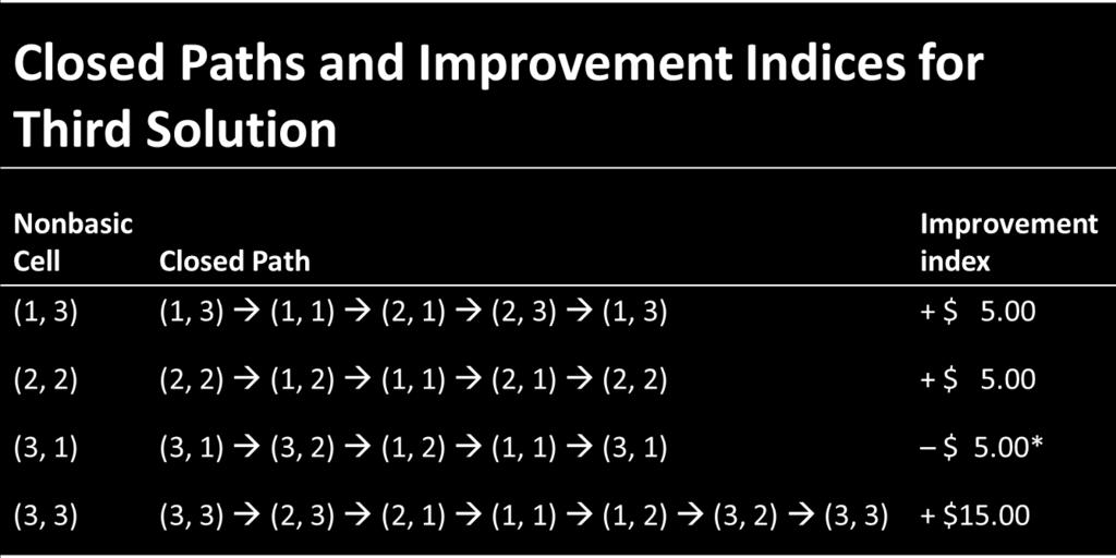
102 102

103 Since all improvement indices are nonnegative in the above table, we conclude that the solution in the above table is optimal. That 103

104 104 is, total cost will be minimized at a value of $3,350 if 55 units are shipped from origin 1 to destination 2 40 units from origin 2 to destination 1 40 units from origin 2 to destination units from origin 3 to destination 1 45 units from origin 3 to destination 2 Alternative optimal solution Given that an optimal solution has been identified for a transportation model, alternative optimal solutions exist if any improvement indices equal 0. If the conditions for optimality exist, allocation of units to cells having improvement indices of 0 results is no change in the (optimal) value for the objective function. In our optimal solution, the above table indicates that allocation of units to cell (2, 2) would result in no change in the total cost. The Assignment Model and Methods of Solution A special case of the transportation model is the assignment model. This model is appropriate in problems which involve the assignment of resources to tasks (e.g, assign n persons to n different tasks or jobs). As the special structures of the transportation model allows for solution procedures which are more efficient than the simplex method, the structure of the assignment model allows for solution methods more efficient than the transportation method. General Form and Assumptions The general assignment problem involves the assignment of n resources (origins) to n tasks (destinations).typical examples of assignment problems include the assignment of salespersons to sales territories, airline crews to flights, ambulance units to calls for service, referees and official to sports events, and lawyers within a law firm to cases or clients. The objective in making assignment can be one of minimization or maximization (e.g., minimization of total time required to complete n tasks or

105 105 maximization of total profit from assigning salespersons to sales territories). The following assumptions are significant in formulating assignment models. Assumption 1 Each resource is assigned exclusively to one task. Assumption 2 Each task is assigned exactly one resource. Assumption 3 For purposes of solution, the number of resources available for assignment must equal the number of tasks to be performed. General Form If x = 1 if resource i is assigned to task j x = 0 if resource i is not assigned to task j c ij = Objective function contribution if resource i is assigned to task j n = number of resources and number of tasks. The generalized assignment model is shown as follows.

106 Notice for this model that the variables are restricted to the two values of 0 (non-assignment of the resource) or 1 (assignment of the resource). This restriction on the values of the variables is quite different from the other linear programming models we have examined. Constraints (1) to (n) ensure that each resource is assigned to one task only. Constraints (n + 1) to (n + n) ensure that each task is assigned exactly to one resource. According to assumption 3, the number of resources must equal the number of tasks for purposes of solving the problem. This condition might have to be artificially imposed for a given problem. Finally, notice that all right-hand-side constants, which are equivalent to s i and d j values in the transportation model, equal 1. The supply of each resource is 1 unit and the demand for each task is 1 unit. 106

107 107 Example (NCAA Referee Assignments) This problem can be formulated as an assignment model. Let x = 1 if team i is assigned to tournament j 0 if team i is not assigned to tournament j The problem formulation is as follows:

108 108 Constraints (1) to (4) assure that each team of officials is assigned to one tourney site only; constraints (5) to (8) assure that each site is assigned exactly one team of officials. Solution Methods Assignment models can be solved using various procedures. These include total enumeration of all solutions, 0 1 programming methods, the simplex method, transportation methods (stepping stone), and special-purpose algorithms. These techniques are listed in an order reflecting increasing efficiency. One of the most popular methods is the Hungarian method. The Hungarian Method The Hungarian method is based on the concept of opportunity

109 109 costs. There are three steps in implementing the method. 1) An opportunity cost table is constructed from the table of assignment costs. 2) It is determined whether an optimal assignment can be made. 3) If an optimal assignment cannot be made, the third step involves a revision of the opportunity cost table. Let s illustrate the algorithm with the following example. Example (Court Scheduling) A court administration is in the process of scheduling four court dockets. Four judge are available to be assigned, one judge to each docket. The court administration has information regarding the type of cases on each of the dockets as well as data, indicating the relative efficiently of each of the judges in processing different types of court cases. Estimated Days to Clear Docket Based upon this information, the court administrator has

110 110 compiled the data in the above table. The above table shows estimates of the number of court-days each judge would require in order to completely process each court docket. The court administrator would like to assign the four judges so as to minimize the total number of court-days needed to process all four dockets. Solution: Step 1: Finding opportunity cost table requires two steps. 1. Identify the least cost element in each row and subtract it from all elements in the row. The resulting table is called row-reduced table. 2. Identify the least cost element in each column and subtract it from all elements in the column. The resulting table is called opportunity cost table. Row-Reduced Cost Table

111 111 Opportunity Cost Table Step 2: Determine whether an optimal assignment can be made: Draw the straight lines (horizontally and vertically) through opportunity cost table in such a way as to minimize the number of lines necessary to cover all zero entries. If number of lines equals either the number of rows or number of columns in the table, an optimal solution can be found. Otherwise, opportunity cost table must be revisited. Identify the smallest number in the table not covered by straight lines. Subtract this number from all the numbers not covered by straight lines and add this number to all numbers lying at the intersection of any two lines. Step 3: Revise the opportunity cost table.

112 112 Revised Opportunity Cost Table Step 2: Determine whether an optimal assignment can be made: As number of lines now of rows, optimal assignment is possible. How to make optimal assignment? Select a row or column in which is only one zero and make an assignment to that cell. Cross out that row and column and repeat step 1.

113 113 Optimal Assignments Select a row/column in which there is only one zero. Make an assignment to that cell. There is only one zero in column 4, thus first assignment is judge 2 to docket 4. Since no further assignment is possible in row 2 or column 4, we cross them off. Again find the row or column in which there is only one zero and repeat the steps above. Continue until all the judges are assigned to respective dockets. Summary of the Hungarian Method Step 1: Determine the opportunity cost table.

114 114 a- Determine the row-reduced cost table by subtracting the least cost element in each row from all elements in the same row. b- Using the row-reduced cost table, identify the least cost element in each column, and subtract from all elements in that column. Step 2: Determine whether or not an optimal assignment can be made. Draw the minimum number of straight lines necessary to cover all zero elements in the opportunity cost table. If the number of straight lines is less than the number of rows (or columns) in the table, the optimal assignment cannot be made. Go to step 3. If the number of straight lines equals the number of rows (columns), the optimal assignments can be identified. Step 3: Revise the opportunity cost table. Identify the smallest element in the opportunity cost table not covered by a straight line. a- Subtract this element from every element not covered by a straight line. b- Add this element to any element(s) found at the intersection of two straight lines. c- Go to step 2. The Hungarian method can be used when the objective function is to be maximized. Two alternative approaches can be used in this situation. The signs on the objective function coefficients can be changed, and the objective function can be minimized, or opportunity costs can be determined by subtracting the largest element (e.g., profit) in a row or column rather than the smallest element.

115 115 Lecture 21,22 Chapter 15: Differentiation This is the first of six chapters which examine the calculus and its application to business, economics, and other areas of problem solving. Two major areas of study within the calculus are differential calculus and integral calculus. Differential calculus focuses on rates of change in analyzing a situation. Graphically, differential calculus solves of following problem: Given a function whose graph is a smooth curve and given a point in the domain of the function, what is the slope of the line tangent to the curve at this point. Limits Two concepts which are important in the theory of differential and integral calculus are the limit of a function and continuity. Limits of Functions In the calculus there is often an interest in the limiting value of a function as the independent variable approaches some specific real number. This limiting value, when it exists, is called limit. The notation lim f(x) = L is used to express the limiting value of a function. When investigating a limit, one is asking whether f(x) approaches a specific value L as the value of x gets closer and closer to a. Notation of Limits The notation lim f(x) = L represents the limit of f(x) as x approaches a from the left (lefthand limit). The notation

116 116 lim f(x) = L represents the limit of f(x) as x approaches a from the right (right-hand limit). If the value of the function approaches the same number L as x approaches a from either direction, then the limit is equal to L. Test For Existence Of Limit If lim f(x) = L=lim f(x) then lim f(x) = L If the limiting values of f(x) are different when x approaches a from each direction, then the function does not approach a limit as x approaches a. Example Determine whether the lim x exists or not? Solution: In order to determine the limit let s construct a table of assumed value for x and corresponding values for f(x). The following table indicates these values.