Application Note. Capacitive Pressure sensor design

Transcription

1 Application Note Capacitive Pressure sensor design

2 Application Note: Capacitive pressure sensor design Version 8/PC Part Number March 2006 Copyright IntelliSense Software Corporation 2004, 2005, 2006 All Rights Reserved. Printed in the United States of America This manual and the software described within it are the copyright of IntelliSense Software Corporation, with all rights reserved. Restricted Rights Legend Under the copyright laws, neither this manual nor the software that it describes may be copied, in whole or in part, without the written consent of IntelliSense Software Corporation. Use, duplication or disclosure of the Programs is subject to restrictions stated in your software license agreement with IntelliSense Software Corporation. Although due effort has been made to present clear and accurate information, IntelliSense Software Corporation disclaims all warranties with respect to the software or manual, including without limitation warranties of merchantability and fitness for a particular purpose, either expressed or implied. The information in this documentation is subject to change without notice. In no event will IntelliSense Software Corporation be liable for direct, indirect, special, incidental, or consequential damages resulting from use of the software or the documentation. IntelliSuite is a trademark of IntelliSense Software Corporation. Windows NT is a trademark of Microsoft Corporation. Windows 2000 is a trademark of Microsoft Corporation. Patent Number 6,116,766: Fabrication Based Computer Aided Design System Using Virtual Fabrication Techniques Patent Number 6,157,900: Knowledge Based System and Method for Determining Material Properties from Fabrication and Operating Parameters

3 Table of contents 1 INTRODUCTION BACKGROUND MEMBRANE DESIGN SAMPLE PROCESS FLOW SURFACE MICRO-MACHINED CIRCULAR MEMBRANE DESIGN THERMO ELECTRO MECHANICAL (TEM) ANALYSIS EXPORTING TO THE TEM MODULE MANIPULATING YOUR VIEW SETTINGS MESH REFINEMENT MATERIAL PROPERTIES, LOADS AND BOUNDARY CONDITIONS Material properties Boundary conditions Loads NATURAL FREQUENCY ANALYSIS STATIC BEHAVIOR Static Stress Analysis with Residual stress effects Incorporating stress gradient effects into the model Capacitance vs. Pressure curve Capacitance vs. Voltage effects Pull-in and membrane collapse Overpressure effects (stress effects) DYNAMIC BEHAVIOR Settling time to a step response Frequency/Spectrum response SYSTEM MODEL EXTRACTION Dominant and relevant modes Strain energy capture Electrostatic energy calculations Exporting the system model SIMULATING YOUR MACROMODEL IN SYNPLE Wiring your circuit Transient Force vs. displacement simulation Compatibility with system modeling tools: PSpice and SIMetrix Result Comparison of SYNPLE, PSpice and SIMetrix SYSTEM LEVEL MODELING SYSTEM LEVEL SIMULATION High level readout circuitry Transistor level design CONCLUSION REVIEW OF CONCEPTS PUTTING IT ALL TOGETHER SUMMARY...93

4 1 Introduction 1.1 Background Pressure sensors and microphones are among the killer applications of MEMS and are rapidly replacing sensors made with more traditional technologies. In this application note, we discuss in detail the various issues in fabrication, design analysis and system modeling of integrated pressure sensor devices. While IntelliSuite and SYNPLE can be used to model capacitive, piezoresistive and piezoelectric sensors, we will focus on electrostatic/capacitive sensing mechanisms in this note. Once the reader grasps the concepts behind the modeling, we are sure that he/she will be able to device sensors based on other detection technologies as well. MEMS based pressure sensors and microphones use an elastic plate (also known as a membrane or a diaphragm as the active mechanical element. As the plate deflects due to the applied pressure, the middle surface (or the neutral axis, is located midway between the top and bottom surfaces of the plate) remains unstressed. The pressure introduces bi-axial stresses in the plate. As the plate moves up, straight lines in the plate that were originally vertical remain straight but become inclined; the intensity of either principle stresses at points on any such line is proportional to the distance from the middle surface, and the maximum stresses occur at the outer surfaces of the plate. Capacitive pressure sensors work by detecting the change in capacitance between a fixed plate and the flexible plate. Piezoresistive pressure sensors work by converting the change in stresses to a change in resistivity of a strategically placed piezoresistor. Piezoelectric sensors work by converting the stresses into a change in electrical potential using a suitable piezoelectric coating. 1.2 Membrane design The reader is referred to the classic Roark s formulas for stress and strain by W.C. Young and R. G. Budynas (Mc Graw Hill) for detailed analytical formulas for plate design. There are several classic papers that the reader may want to peruse for a good understanding of pressure sensors. These include: [1] A simulation program for the sensitivity and linearity of piezoresistive pressure sensors. Liwei Lin, JMEMS, December 1999 [2] Solid state capacitive pressure transducers. WH Ko. Sensors and Actuators, vol 10, 1986 Analytical solutions are available for an unstressed membrane. These can be used as a starting point for the design. In reality, full Finite Element/Boundary Element (FE/BE) based calculations are needed to incorporate processing related effects such as residual stresses and strain gradients. These are important effects that significantly effect the membrane deflection and can lead to unwanted effects such as membrane bi-stability (oil-can effect). As a starting point for the pressure sensor design, consider a circular membrane with a radius R and thickness h. The deflection of the circular membrane is given by the equation: W()= r p ( 49.6D R2 r 2 ) 2 Eh 3 where D = 12 1 ν 2 ( ) The maximum deflection of the membrane is given at the center of the membrane when r = 0 as:

5 The maximum stress in the membrane is given as: ( W max = 1 ν 2 )R Eh 3 p σ max = 1.25pR2 h 2 For CMOS integrated poly-silicon and silicon pressure sensors, the typical material properties are E = GPa, Poisson s ratio = The density of silicon is 2320 kg/m 3. In most surface micromachined processes the poly-silicon thickness is between 1-2 µm. The capacitor gap in integrated pressure sensors is between 1-2 µm depending upon the choice of sacrificial material. Since the capacitance between the electrodes is a non-linear function of the gap, most sensor designers like to work in the linear range of pressure-displacement response. The maximum deflection at full scale is chosen such that the maximum deflection does not exceed 25-30% of the capacitance gap. Assuming mean values of membrane thickness of 1.5 µm and capacitor gap of 1.5 µm, let us limit the maximum deflection of the membrane at full scale to 0.4 µm. Based upon this criteria we can estimate the membrane sizes for different full scale pressures using the expression R = 4 w max 4.13Eh 3 (1 υ 2 )p The table overleaf gives a sample calculation of the radius of the device for different pressures. 2

6 Material Properties E 1.69E+11 Pa Nu 0.22 Density 2320 kg/m3 Dimensions Thickness 1.50E-06 m Capacitor gap 1.50E-06 m Maximum stroke 0.28 of gap Max stroke 4.20E-07 m Dimensional estimates (radius) Max stroke (w_max) 4.20E-07 m Pressure (bar) Radius (µm) Maximum stress (Mpa) Table 1 Pressure sensor design 3

7 2 Sample process flow 2.1 Surface micro-machined circular membrane design 1. Open the Pressure Sensor Simulation file (ProcessFlow.fab) in IntelliFAB using the default process database. The figure below shows the process flow for the surface micromachined pressure sensor. This can be done by: a) Launching IntelliFAB b) Clicking on the left hand side of the interface (white) and choosing File > Open Database > matfab.db c) Click on the right hand side of the interface (blue) this activates the fabrication portion of the interface open the Fabrication Process flow by choosing File > Open Fab > IntelliSuite\Training\Application_Notes\Capacitive_Pressure_Sensor\Process\ProcessFlow.fab. d) You will see the interface shown below. Figure 1 Process flow for the surface micromachined pressure sensor 4

8 2. Explore the process table by double clicking on each of the process steps and looking at the process parameters. In particular, when you open a Lithography step (Definition UV.) make sure you take a look at the mask layout associated with the step. You can do it by clicking the Layout button as shown in the figure below. Figure 2 Spend some time exploring the process parameters. Make sure you take a peek at the Mask layouts associated with the process by clicking the Layout button. 5

9 3. Visualize the process by choosing Construct > Visualize. Step through the process visualization using the Start, Previous and Next buttons on the interface. a) Note that the Last step of sacrificing the silicon wafer was added to isolate the device for ease of simulation, in reality the silicon wafer is never sacrificially etched! Figure 3 Visualize the device fabrication 6

10 3 Thermo electro mechanical (TEM) Analysis 3.1 Exporting to the TEM module You can start the simulation by exporting the fabrication sequence into the ThermoElectroMechanical module. You can do this by Clicking Simulate menu and choosing the ThermoElectroMechanical menu entry. Figure 4 Export to the TEM module Save the Analysis file (.save) in a convenient directory (make sure that there are no spaces in the folder or file name). Figure 5 Save the analysis file (.save) in a convenient location make sure that the file, folder and path names do not have spaces in them. Use an underscore character instead of a space. IntelliSuite will automatically create a Finite Element Meshed model of the structure and open it in the TEM module. 7

11 3.2 Manipulating your view settings Since surface micromachined MEMS devices are typically just a few thick, they appear to be very flat in the initial view in TEM. TEM gives you the capability to independently set X, Y and Z default zoom factors. 1. You can use the Shift + Up arrow and Shift + Down arrow to zoom in and out. Ctrl + Up arrow and Ctrl + Down can be used to rotate the device. You can also use your mouse to manipulate the device in the 3D space. 2. You can use the View > Zoom > Define to set your view setting in X, Y and X directions. Figure 6 Zoom Define Dialog allows you to set independent X, Y and Z zoom factors. Choose a Z zoom factor of 100 in this case. 3. Feel free to explore the different view options available and make yourself comfortable with the keyboard shortcuts and mouse movements to manipulate the device the in 3D space. 8

12 4. The view of the pressure sensor should look similar to the figure below Figure 7 Initial view of the device after setting the appropriate zoom factors 3.3 Mesh refinement Click Mesh Auto Enter 10 in the maximum mesh size dialogue 9

13 3.4 Material Properties, Loads and Boundary conditions In order to perform analyses in the TEM module, you can follow the menus sequentially from View to Result. The actions that are to be performed are laid out in a logical progression. The menus will allow you to choose your simulation settings, check and modify material properties, apply loads and boundary conditions, mesh the device, and explore the simulation results Material properties The material properties of the device can be set by Selecting the Materials menu. Materials > Check/Modify. You can click on an entity to set the material properties. 10

14 Figure 8 Use Material > Check/Modify to modify the material properties 11

15 Figure 9 Selected entities are highlighted in red. For instance clicking on the word density will bring the modify density dialog which allows you to specify either a constant or a variable (with temperature) density Figure 10 You can apply residual stresses (constant) or high order variable stress gradient profiles Boundary conditions You can set the boundary conditions by selecting the appropriate degree of freedom of a particular entitiy and clicking on the appropriate boundary. Make sure you fix all of the fixed boundaries of the device as shown in thefigures below. 12

16 Figure 11 Fixed boundary conditions for the pressure sensor. The bottom electrode and the surface in contact with the silicon are fixed Click Boundary.SelectionMode CheckOnly Click...Boundary Fixed All the Fixed Boundaries will be highlighted Loads IntelliSuite allows you to apply a large number of loads to the device. These range from forces, pressures, Coriolis forces, temperatures and other stimuli. The loads can be constant loads, time varying loads or frequency varying loads. We will revisit the load application in static analysis. 3.5 Natural frequency analysis Let us explore the first 5 modes of the device. Frequency analysis allows you to quickly check your model setup and mesh convergence information. Since AC/Frequency analysis results can be performed quickly, they are often used to make sure of the model accuracy. 1. Set the simulation settings by choosing Simulation > Simulation Settings Figure 12 Accessing Simulation settings 2. Set the simulation settings as below. Click Apply and OK 13

17 Figure 13 Simulation settings for frequency analysis 3. Start the simulation by choosing Analysis > Start Frequency Analysis. Wait for the analysis to complete this should take 1-5 minutes depending upon your machine 4. Explore the results by choosing Result > Natural Frequency Natural Frequency 14

18 5. View mode animations by choosing Result > Mode Animation 3.6 Static behavior Static Stress Analysis with Residual stress effects To model the effect of a Residual Stress of 20Mpa on the diaphragm, first change the simulation settings as shown in the Figure below 15

19 Click Apply OK Click Material Check/Modify 16

20 Select the Diaphragm and a dialogue will appear as shown in the Figure below. Double Click Stress Enter 20 for the New Value of STRESS (Tensile stress of 20Mpa) Click OK twice to close both the dialogues. Click Analysis Start Static Analysis 17

21 Click Results Z Displacement Incorporating stress gradient effects into the model Click Material.Check/Modify 18

22 Click on the diaphragm Double Click Stress Click Variable Enter the stress values as shown in the Figure below Click Analysis..Start Static Analysis Click Result Displacement...Z 19

23 3.6.3 Capacitance vs. Pressure curve Click Simulation Simulation Setting Change the simulation settings as shown in the Figure below. 20

24 Click Apply OK We will remove the stress gradient in the model and include a constant residual tensil stress of 20Mpa. Click Material Check/Modify Click on the Diaphragm Double Click Stress...Constant Change the value as shown in the Figure below Click Loads.SelectionMode Pick on Geometry Click...Loads Voltage Entity 21

25 Select the Diaphragm Enter 0V as shown in Figure below Click OK Click on the Bottom Doped Electrode Enter 0V for the Voltage as shown in Figure below 22

26 Click OK Click.Loads Pressure Face Select the top face of the diaphragm Enter 0 MPa for the Pressure as shown in the Figure below 23

27 Click OK Click Analysis Start Static Analysis Once the analysis is complete, Click Result Displacement z 24

28 The displacement should be due to the residual stress in the diaphragm. Click Result Capacitance This is the initial capacitance between the diaphragm and the electrode. The capacitance result is in the form a capacitance matrix. The capacitance between Entity 1 and Entity 2 or vice versa is the capacitance of interest. The capacitance results are in the form of a matrix. Entity1 Entity 1 capacitance is C11, which is the capacitance of Entity 1 with respect to infinity. Entity 1-Entity2 /Entity2-Entity1 are the capacitances of Entity 1 w.r.t Entity 2. Entity2-Entity2 is the capacitance of Entity 2 w.r.t infinity. Increase the pressure on the diaphragm and find the change in capacitance: Click Loads Pressure Face Select the top face of the diaphragm as shown in the Figure below Enter a Pressure value of MPa 25

29 Click Analysis Start Static Analysis Click Result Displacement Z Click Result Capacitance 26

30 Repeat the above steps for different values of Pressure and Plot the Pressure vs. Capacitance values to characterize the response of the capacitive pressure sensor. Please compare the results with the plot below. Capacitance vs. Pressure y = x R 2 = Capacitance [ff] Pressure [MPa] 27

31 Please note the Z-displacement for each of the Pressure values and compare the results with the plot below Displacement vs. Pressure 7.00E E-01 Displacement [Microns] 5.00E E E E E E Pressure [MPa] Capacitance vs. Voltage effects Remove the Pressure loads on the Diaphragm. Click Loads SelectionMode Delete All Click Loads Pressure Face Click Loads SelectionMode Pick on Geometry Click Loads Voltage Entity Select the diaphragm (yellow entity) Enter 10V We will retain 0V on the Doped bottom electrode (green entity) Click Analysis.StartStaticAnalysis Once the simulation is complete Click Result Displacement Z 28

32 Click Result Capacitance Repeat this simulation by varying the voltage on the yellow entity (diaphragm) The results form this information can be used to arrive at the C vs. V response. Please match the results from the simulation with the results in the Figure below. 29

33 Capacitance [MicroF] 2.40E E E E E E E E E E-08 Capacitance vs. Voltage Voltage[ V] 0 psi 50 Psi The capacitance should not change for the pressure range 0-50 Psi Pull-in and membrane collapse For Pull-in analysis, we will need to perform a Thermo-Electro-Mechanical-Relaxation analysis with Contact. The contact faces would be the bottom face of the yellow entity (diaphragm) and the top face of the green entity (bottom doped electrode). Click Simulation Simulation Settings Change the simulation settings as shown in the Figure below 30

34 Click Apply OK Click Loads Voltage Entity Select the Yellow entity (diaphragm) Click InputValueRange Enter the values as shown in the Figure below: 31

35 Click Boundary SelectionMode PickonGeometry Click.Boundary Contact FacePairDefinition Face A 32

36 Select the bottom face of the diaphragm (yellow entity) as shown in the Figure below Click OK Click Boundary Contact FacePairDefinition FaceB Rigid Select the top face of the Bottom electrode (green entity) 33

37 Click OK Click Boundary.Contact FacePairDefintion Complete Pair DoubleClick.Disabled To Enable Face 89 and 2 34

38 Click Accept OK Click Boundary Contact FacePairDefinition VerifyContactPairs Contact Pair 1 should be activated Click OK to activate the pair Click Analysis.StartStaticAnalysis Click Result 2DplotElectroMechanicalAnalysis XCoordinate Voltage Click Result 2DplotElectroMechanicalAnalysis YCoordinate Z-displacement A 2D plot will appear as shown in the Figure below 35

39 The voltage sweep was from 300V to 1000V. This can be fine tuned to 0 V to 650V with 50V increment. The simulation will take longer as more points need to be computed Overpressure effects (stress effects) Click Simulation SimulationSetting Reset the simulation settings as shown in the Figure below 36

40 Click Apply OK Click Loads Voltage Entity Select the yellow entity (diaphragm) Click SingleValueInput Enter 0V for the voltage input 37

41 Click Loads Pressure Face. Enter MPa (1000 psi) for the pressure load. 38

42 3.7 Dynamic behavior Settling time to a step response We will perform a dynamic Stress/Displacement (Direct Integration) analysis to determine the settling time for the pressure sensor and the influence of stiffness/mass damping on the settling time Click Simulation.SimulationSettings (to reset the simulation settings as shown in the Figure below) 39

43 Click Apply OK Click Material DampingDefinition (Define Mass and Stiffness damping according to the Figure below) for a damping factor of

44 Click Apply OK Click Loads Amplitude vs. time.tabular Click Loads Pressure Face Select the top face of the diaphragm (yellow entity) Complete the Time vs. Pressure table as shown in the Figure below Click OK Click Analysis StartDynamicAnalysis Click Result 2DPlotMechanicalAnalysis.Maximum.Displacement Z The 2D plot will appear as shown in the Figure below. 41

45 3.7.2 Frequency/Spectrum response The spectrum analysis is a frequency sweep analysis. This gives the displacement results for the model over a specified frequency range. The Spectrum analysis results should match the static frequency analysis results. Click.Simulation.SimulationSetting Change the simulation settings as shown in the Figure below 42

46 Click Loads...SelectionMode.PickonGeometry Click Loads Amplitudevs.Time Tabular Set the loads according to the Figure below 43

47 (DoubleClick on 1 / 2 to Enter the Frequency and Pressure) Click.OK Click Material ModeDamping Check if the ModeDamping is set to 0.01 for Mode 1. Click OK Click.Analysis.StartDynamicAnalysis Once the Analysis is complete Click Result 2DPlotMechanicalAnalysis Maximum Displacement Z The 2D plot should appear as shown in Figure below 44

48 Compare this value with the static Frequency results (shown in Figure below) 45

49 3.8 System model extraction SME is a means by which a full three-dimensional meshed numerical model of a multi- conductor electromechanical device without dissipation can be converted into a reduced-order analytical macromodel that can be inserted as a black-box element into a mixed signal circuit simulator. This process is based upon the energy method approach, in that we shall construct analytical models for each of the energy domains of the system and determine all forces as gradients of the energy. The energy method approach has the advantage of making this process modular, enabling us to incorporate other energy domains into our models in the future. Another beneficial side effect of energy methods is that the models we shall construct are guaranteed to be energy conserving, because each stored energy shall each be constructed as an analytical function, and all forces shall be computed directly from analytically computed gradients. The SME process also has the advantage of being able to be performed almost entirely automatically, requiring the designer only to construct the model, run a few full threedimensional numerical computations, and set a few preferences a priori. Above all, this process has the ultimate benefit of constructing models that are computationally efficient, allowing their use in a dynamical simulator. Our first task is to reduce the degrees of freedom of the system. Rather than allow each node in a finite element model to be free to move in any direction, we constrain the motion of the system to a linear superposition of a select set of deformation shapes. This set will act as our basis set of motion. The positional state of the system will hence be reduced to a set of generalized coordinates, each coordinate being the scaling factor by which its corresponding basis shape will contribute. Next, we must construct analytical macromodels of each of the energy domains of the system. In the case of conservative capacitive electromechanical systems, these consist of the electrostatic, elastostatic, and kinetic energy domains. These macromodels will be analytical functions of the generalized coordinates. (As we will see in Section Using Mode Shapes as a Basis Set, some of these energy domains will be determined as a byproduct of modal analysis, avoiding the need for explicit calculation.) We can then use Lagrangian mechanics in order to construct the equations of motion of the system in terms of its generalized coordinates. Finally, we can translate these equations of motion into an analog hardware description language, thereby constructing a black-box model of the electromechanical system that can be inserted into an analog circuit simulator. The Figure below gives the Flow Chart for the conversion of an FEA model into an equivalent system level mode. 46

50 Some of the key equations used for the conversion process are discussed in this section. In general, the deformation state and dynamics of mechanical system can be accurately described as the linear combination of mode shape function or modal superposition. Ψ ext (x,y,z,t) =Ψ initial (x,y,z) + q i (t) ψ i (x,y,z) where Ψ ext represents the deformed state of structure, Ψ initial represent the initial equilibrium state (derive from the residual stress without external loads), ψ i (x,y,z) represents the displacement vector for the i th mode, q i represents the coefficients for the i th mode, which is refered as scaling factor for mode i. The modal superposition based reduce order modeling method is to solve each equation m i 2 q i / t 2 + 2ξ i ω i m i q i / t + U m (q)/ q i - Ue(q)/ q i - ψ i F j = 0 where m i is the i th mode generalized mass, ξ i is the linear modal damping ratio, ω i is the i th eigenfrequency, ψ i is the ith modal shape function (the displacement vector for the ith mode). ψ i F j is sum over all the nodes of the external node force weighted by the mode shape. U m is the strain energy, U e is the electrostatic energy, U e can be described as U e = 1/2 (C* V 2 ) The modal superposition method is efficient since just one equation per mode and one equation per involved conductor are necessary to describe the coupled system entirely, which is also applied to both linear and nonlinear geometry. The modal superposition based reduced order modeling procedure includes the following steps: 47

51 Find out Modal Contribution. In this step, perform the standard electromechanical relaxation analysis and solve the initial deformed state (derive from the residual stress without external loads) and the final deformed state (with mechanical loads and applied voltage). Then use the QR factorization algorithm to determine the mode contribution for the deformed state. Calculate the relationship of Strain Energy vs modal amplitudes. In this step, calculate the selected mode Strain Energy vs modal amplitudes. Calculate the relationship of mutual capacitance vs Modal amplitudes. In this step, calculate the selected mode mutual capacitance vs modal amplitudes. From step 2 and 3, user can obtain U m (q)/ q i and Ue(q)/ q i respectively. For the current pressure sensor device, the following procedure describes the steps to extract the macromodel Dominant and relevant modes Click Simulation SimulationSettings Reset the Simulations according to the Figure below 48

52 Click Material ModeDamping Definition Enter 5 for the mode number Click Analysis StartExtractMacroModel 49

53 Once the analysis is complete Click Results Macromodel ModalContribution Since Mode 1 has the maximum contribution (which is the case for most cases), the rest of the Modes can be disabled (Double Click on the Mode number to disable/enable a mode) but we will retain all the 5 modes for this case. Click OK From the Modal contribution results, we notice that the contribution from Mode 1 is the maximum. For the Strain Energy Capture and the Mutual Capacitance capture, the scaling factor needs to be selected in the simulation settings. The default scaling factor for all the modes is 1, which will work for most of the cases. The only criterion for selecting the scaling factor is that the scaling factor should be greater than the modal contribution for a given mode. For a modal contribution , the scaling factor can be chosen as 1 and the scaling factor will range from -1 to Strain energy capture Click Simulation Simulation Settings Change the simulation settings as shown in the Figure below 50

54 Click Apply OK. Click Material Mode Damping Definition. Enter 5 for the Mode number Specify the Mode Damping as 0.01 for the 5 modes. Click Simulation Start Extract Macromodel Once the simulation is complete Click Result Macromodel.Strain Energy vs. Modal Amplitudes Double Click on 1 in the Model column to enable the plot option for mode 1 and then click OK. A plot of the strain energy for mode 1 over the operating range will appear as shown in Figure below 51

55 Similarly, plots for Mode 2, 3, 4 and 5 can be generated using the same procedure. 52

56 Click File Exit Click OK 53

57 3.8.3 Electrostatic energy calculations For the Mutual Capacitance vs. Modal Amplitudes calculations: Reset the Simulation settings as shown in the Figure below: Click Simulation.Simulation Settings Click Apply OK Click Simulation Start Extract Macromodel Once the simulation is complete Click File Save Click Boundary Macromodel Representative Nodes. 54

58 Select the node as shown in the Figure below (Highlighted node) Node 5715 We will apply node forces on the selected node during the simulations in SYNPLE. The macmodel.out file stores the information on the representative node Exporting the system model The four files str.out, curr.macmodel, macmodel.out and TEST.save in the current working directory provide all the information required for the macro model generation. User can manually copy the four files to a different directory for use with SYNPLE module and exit the Thermal electro-mechanical module, or keep the TEM module open and start the SYNPLE module Run the SYNPLE module and incorporate the macromodel information generated from the TEM module 55

59 3.9 Simulating your Macromodel in SYNPLE Wiring your circuit Click Start Programs IntelliSuite SYNPLE In the SYNPLE simulator, on the left side you have a list of available elements, categorized into Electrical Elements, Mechanical Elements, MEMS Elements. On the right side you have the 2D grid for your schematic as shown in the Figure below Click MEMSDevices.Click the Macromodel for TEM element and drag the element to the grid on the right side as shown in Figure below 56

60 Click the Macromodel template on your right Click Schematic IncludeReducedOrderMacromodel Select the curr.macmodel file (This file is saved in IntelliSuite\Training\Application_Notes\Capacitive_Pressuer_Sensor\SystemModeling) Click Open 57

61 To complete the circuit for the static analysis, we will need the following electrical and general elements: A DC source element from the Electrical Devices library A Ground element from the Electrical Devices library 2 Constant and 4 Output terminal elements from the General devices library Please wire the elements as shown in the Figure below If the wires are connected correctly, a name will automatically appear for the wire. The name can be changed by double clicking on the wire. Select the wire button as shown in the Figure below (arrow) Click and Drag between the nodes on the respective elements to connect them with a wire. Please save the file at regular intervals Please refer the wiring section in the Getting Started with SYNPLE manual for more instructions on wiring and common errors. Once the wiring is complete Click File Save/Save As NOTE: Please save file in the same folder as the other files (curr.macmodel, macmodel.out, str.out) All system modeling files are saved in IntelliSuite\Training\Application_Notes\Capacitive_Pressuer_Sensor\SystemModeling Double Click the Macromodel template/element on the schematic Set the properties of the macromodel as shown in the Figure below. 58

62 Click OK Double Click the DC source and set VDC as 5.This voltage has to be less than the pull-in voltage. We will need a minimum DC voltage Double Click the Constant element connected to pin Fz1 and modify the properties as shown below 59

63 We are defining a 650µN load in the z-direction For the other Constant element leave the default values (0) for c, c1 and c2. Click...DC 60

64 We will now specify a DC sweep (Parametrize the applied force) for the force/loading condition. Click Parametric Variation Settings (DC Sweep) Click Add (in the parametric variation window) Select the parameter c_of_force Double Click on the Parameter and change the settings as shown in the Figure below We are sweeping the force linearly from 0N to 0.001N with the average value being 650 µn 61

65 Click Done Click Close Leave the DC Time as 0 Click Signals Select the Signals shown in Figure below 62

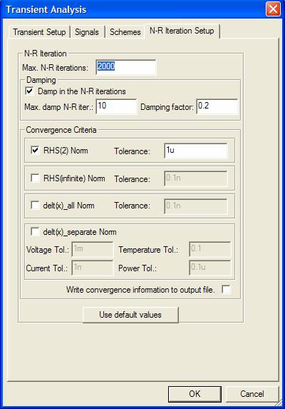
66 The first 7 signal names are names of the wires shown in Figure below Click N-R Iteration Setup and reset the settings as shown in Figure below 63

67 Click OK to start the analysis Once the analysis is complete, the signal manager with the selected signals will appear Double Click the signals to view the plot/result Eg: Double click on Z1 The plot of Z1 vs. Force will appear as shown in the Figure below 64

68 This simulation file has been saved as Pressure_sensor1.ssc and is present in IntelliSuite\Training\Application_Notes\Capacitive_Pressure_Sensor\SystemModeling Transient Force vs. displacement simulation We will perform a transient analysis for with the same macromodel We will need to remove the constant element assigned to Fz1 and replace it with a General Pulse Source (1p) as shown in Figure below This element is available in the General Devices category Double click on the General Pulse element and change the properties as shown in the Figure below 65

69 We are applying a 2µsec pulse of 650µN Click OK Click Transient Reset the simulation settings as shown in the Figures below: 66

70 67

71 Click OK To start the simulation Once the simulation is complete Double Click on signals in the Signal manager to view the transient results 68

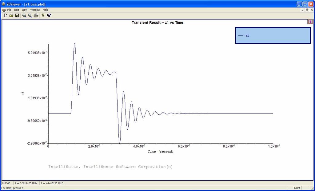
72 Eg: Double click on the Z1 signal to view the transient displacement results: Click File exit The transient simulation file is saved as IntelliSuite\Training\Applicaton_Notes\Capacitive_Pressure_Sensor\SystemModeling\pressure_sensor1tra ns.ssc 69

73 3.9.3 Compatibility with system modeling tools: PSpice and SIMetrix Result Comparison of SYNPLE, PSpice and SIMetrix The structure has 2 electrodes, which are connected to a 5 volts DC source and ground respectively. An external pulse force acts at z-direction on the reference node. We are monitoring the z-direction displacement in AC Sweep, DC Sweep and Transient analysis. AC Sweep: Swept frequency from 100 Hz to 100 MHz DC Sweep: Swept the external force from 0 to 1 mn Transient: Applied a 650 µn pulse force as shown on the plot. 70

74 DC Sweep: SYNPLE PSpice 71

75 SIMetrix 72

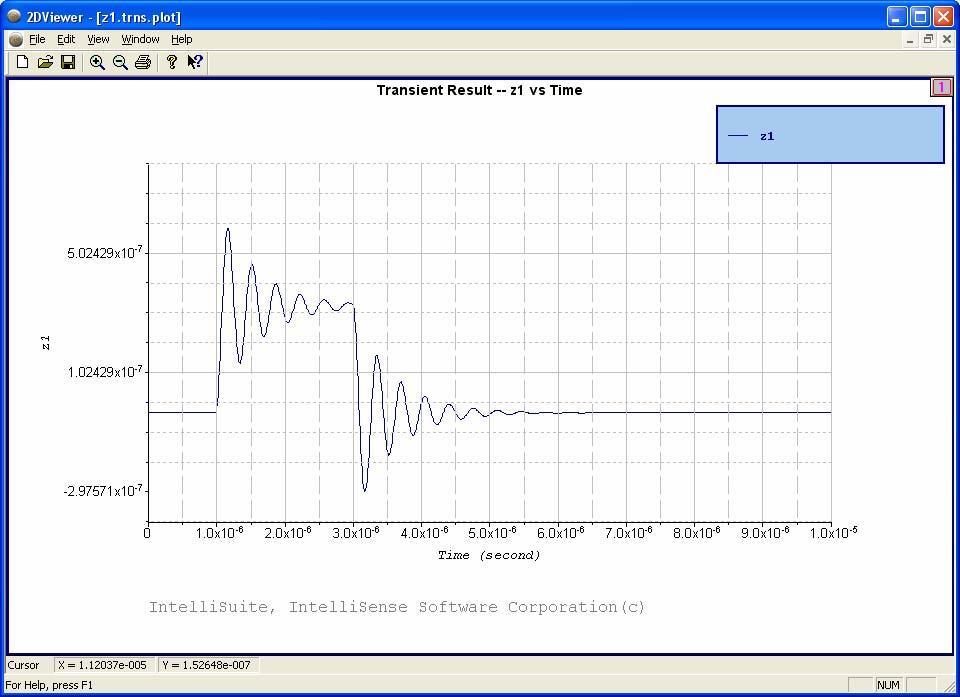
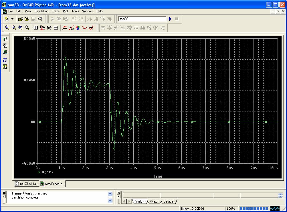
76 Transient: SYNPLE PSpice 73

77 SIMetrix: The SIMETRIX circuit files are saved in IntelliSuite\Training\Application_Notes\Capacitive_Pressuer_Sensor\SystemModeling \EDALinker\SIMetrix The EDALinker.exe file is present in IntelliSuite\Training\Application_Notes\Capacitive_Pressuer_Sensor\SystemModeling\EDALinker 74

78 AC Analysis: SYNPLE Magnitude Phase 75

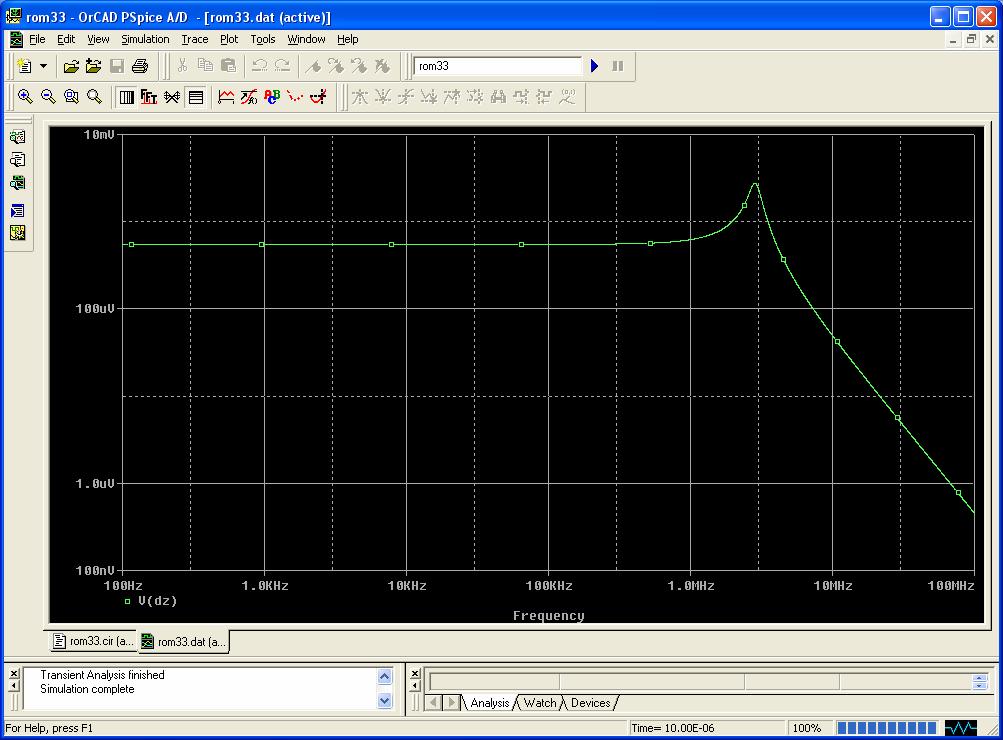
79 PSpice 76

80 SIMetrix 77

81 4 System level modeling 4.1 System level simulation High level readout circuitry Sigma Delta Modulator: This example is for a second order Sigma delta modulator. The input to the modulator is a sine wave and the output is a digital output carried by a clock signal. This Sigma Delta Converter can be interfaced with the MEMS Macromodel to simulate the complete control circuit for the MEMS device. Start the SYNPLE module. Click on File.Open.C:/IntelliSuite/SYNPLE/Examples/ElectricalCircuitExamples/First order sigmadelta modulator/sigdel5.ssc The Sigma-delta modulator file The circuit should appear as shown in Figure below with the operational amplifiers, switching circuits and capacitors. 78

82 Second Order Sigma-Delta Modulator We will perform a transient analysis with the modulator with a sine wave input. AC Input Signal Double click on the AC input signal to view the amplitude and frequency of the signal as shown in Figure 3 and Figure below. 79

83 AC input signal Click OK to close the dialog. Click on the Transient Analysis button 80

84 Click on the Transient Analysis option The Transient Analysis Dialog will show up as shown in Figure below. Transient Analysis settings 81

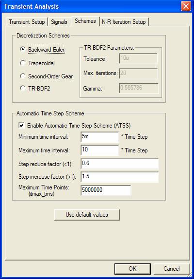
85 Please reset the Simulation settings as shown in Figures below. Signals D Discretization Schemes Click OK to Start the Transient Simulation. In Figure 7, we select only Vin as the Signal to View. We will first visualize the input Sine Wave and run the simulation again to view the output Digital Signals. The simulation should complete and a Signal Manager dialog with the signal to be viewed will appear. This is shown in Figure 10. N-R Iteration Setup 82

86 Simulation completes and the Signal Manager appears. Double Click on Vin in the Signal Manager and the input sine wave signal will appear as shown in Figure below. Input Signal Vin Click on the Transient Analysis Button again and reset the settings on the dialog as shown in Figure below 83

87 Unselect Vin and Select y and yb Click OK to start the Analysis Once the analysis completes, Click on the signals y and yb in the signal manager window. The Digital Outputs should appear as shown in Figures below. 84

88 Digital Output y Digital Ouput yb y and yb can be located on the circuit and the outputs are inverse of each other. This example was for a second order sigma-delta modulator. The FirstOrderSigmaDeltaModulator folder has more examples. 85

89 4.1.2 Transistor level design This capacitive pressure sensor was built in SYNPLE using a variety of MEMS and electrical elements available in the SYNPLE library. The circuit is designed to amplify the capacitance signal of the pressure sensor. The circuit output is an amplified Analog signal for an applied pressure pulse. The Analog signal can be sent through a Sigma Delta Converter for an equivalent digital output. Click...File Open balanced_demodulator_bsim.ssc File is located in IntelliSuite\Training\Application_Notes\Capacitive_Pressuer_Sensor\SystemModeling Double Click any Bsim to check the properties of the transistor 86

90 Variables l and w are highlighted as they are global variables for all Bsim s in the circuit. Note : To define Global variables: Click Schematic Global Variable Manager Click Add 87

91 Define the value and the variable name Click OK Close Bsim simulation contd Double click on the Pressure input to the sensor 88

92 The properties of the input signal should be changed according to the Figure below 89

93 We are defining a 120Pa pressure pulse from 0 sec to 120µsec. (The input is in the form of a triangular pulse and the loading condition is during the linear increase (first half t0 to t1 of the triangular pulse) Click OK Click Transient Set the simulation settings as shown in the Figures below 90

94 91

95 Click OK Once the Simulation is complete Double click on Pressure in the Signal Manager window The Pressure input to the sensor will be displayed as shown in Figure below Double Click Cap_of_Cs1 The capacitance output of the pressure sensor will be displayed as shown in Figure below 92

96 5 Conclusion 5.1 Review of concepts A surface micro-machined circular capacitive pressure sensor was designed and simulated in both the device level and the system level. The layout was designed in IntelliMask and the process simulation and the 3D structure were realized in IntelliFab. The device level simulation performed on the device can be categorized into frequency analysis, static analysis, dynamic analysis and system model extraction. The static analysis involved residual stress analysis, stress gradient analysis, capacitance vs. pressure analysis, capacitance vs. voltage analysis, pull-in analysis, and overpressure analysis. The dynamic analyses involved dynamic pressure analysis and spectrum analysis. System model extraction involved extraction of relevant modes, strain energy and electrostatic energy. A Transient Force vs. displacement analysis was performed on the system model of the pressure sensor in SYNPLE and the results were compared with the results from SIMETRIX and PSPICE. System level analysis involved sigma delta modulator analysis and transistor level design. The sigma delta modulator could be potentially connected to the macromodel output to convert the analog output into an equivalent digital signal. The Transistor level design was for a pressure sensor designed using a collection of MEMS and Electrical elements including BSims (Transistors). The properties of the transistor can be varied according to the information available from the process flow. 5.2 Putting it all together We will now review the results from each of the analyses and the significance of the results. The natural frequency analysis was done to determine the natural frequencies for the first five modes. These results were further used to validate the results from the frequency/spectrum analysis. The static stress and residual stress analysis were performed to determine the effects of these stresses on the device behavior. The Capacitance vs. Pressure analysis was performed to determine the change in capacitance for applied pressure and characterize the capacitive response of the device. The Capacitance vs. Voltage analysis was performed to determined the displacement and the resulting capacitance caused by varying the voltage on the device. The pull-in and membrane collapse analysis were performed to determine the pull-in voltage for the device. Overpressure effects were analyzed to determine the device behavior at very high pressure loads. The dynamic analysis was performed on the device to determine the settling time for the sensor for a specific force/pressure pulse and damping factor. The system model of the pressure sensor was extracted to perform a system level analysis in SYNPLE and in EDA tools such as SIMETRIX and PSPICE. The results from SYNPLE, SIMETRIX and PSICE were compared for a transient Force vs. Displacement analysis. 5.3 Summary A Capacitive pressure sensor was designed successfully both at the device level and the system level. The methodical approach to design a surface micromachined capacitive pressure sensor from Layout through process simulation, Frequency Analysis, Static Analysis, Dynamic Analysis, System Model Extraction, SPICE extraction, System level simulation in SYNPLE, transistor level simulation in SYNPLE and comparison of results between SYNPLE.SPICE and SIMETRIX has been discussed in detail in this application note. 93