Chapter 4 Image Enhancement in the Frequency Domain
|
|
|
- Florence Davis
- 5 years ago
- Views:
Transcription
1 Chapter 4 Image Enhancement in the Frequency Domain Yinghua He School of Computer Science and Technology Tianjin University
2 Background Introduction to the Fourier Transform and the Frequency Domain Smoothing Frequency-Domain Filters Sharpening Frequency Domain Filters Homomorphic Filtering Implementation
3
4 Background Introduction to the Fourier Transform and the Frequency Domain Smoothing Frequency-Domain Filters Sharpening Frequency Domain Filters Homomorphic Filtering Implementation
5 The One-Dimensional Fourier Transform and its Inverse The Two-Dimensional Fourier Transform and its Inverse Filtering in the Frequency Domain Correspondence between Filtering in the Spatial and Frequency Domains
6 The Fourier transform Fu of a single variable continuous function f is defined by the equation Where j F u 1 j πu f e 2 d Conversely given Fu we can obtain f by means of the inverse Fourier transform f j πu F u e 2 du These two equations comprise the Fourier transform pair.
7 These equations are easily etended to two variables u and v: F u v j 2π u+ vy f y e ddy And similarly for the inverse transform f y j 2π u+ vy F u v e dudv
8 The Fourier transform of a discrete function of one variable f 012 M-1 is given by the equation M 1 F u 1 f e j2πu / M for M M Similarly given Fu we can obtain the original function back using the inverse DFT: f M 1 u 0 F u e j2πu / M u for M 1
9 The concept of the frequency domain follows directly from Euler s formula: θ e j cosθ + j sinθ Substituting this epression into Eq and using the fact that cos θ cosθ gives us F u M 1 M 1 0 f [ cos 2πu / M j sin 2πu / M ] for u M 1
10 In the analysis of comple numbers we find it convenient sometimes to epress Fu in polar coordinates: Where F u F u e [ ] 2 2 R u I 1/ 2 F u + u jφ u Is called the magnitude or spectrum of the Fourier transform and
11 Is called the phase angle or phase spectrum of the transform. Another quantity that is used in this chapter is the power spectrum defined as the square of the Fourier spectrum: tan 1 u R u I u φ u I u R u F u P +
12 The first value of the sampled function is then f 0. The kth sample gives us f 0 + kδ. When we write fk it is understood that we are utilizing shorthand notation that really means f 0 + kδ.
13 f is then understood to mean Fu is then understood to mean and are inversely related by the epression 0 f f Δ + Δ u u F u F Δ Δ Δ u Δ M u Δ Δ 1
14
15 The One-Dimensional Fourier Transform and its Inverse The Two-Dimensional Fourier Transform and its Inverse Filtering in the Frequency Domain Correspondence between Filtering in the Spatial and Frequency Domains
16 The discrete Fourier transform of a function image fy of size M*N is given by the equation Given Fuv we obtain fy via the inverse Fourier transform given by the epression for 012 M-1 and y012 N / / 2 1 M N y N vy M u j e y f MN v u F π / / 2 M u N v N vy M u j e v u F y f π
17 The Fourier spectrum phase angle and power spectrum: Where Ruv and Iuv are the real and imaginary parts of Fuv respectively. [ ] 2 1/ 2 2 v u I v u R v u F + tan 1 v u R v u I v u φ v u I v u R v u F v u P +
18 It is common practice to multiply the input + y image function by 1 prior to computing the Fourier transform. Due to the properties of eponentials it is not difficult to show that I [ ] + y f y 1 F u M / 2 v N / 2 Where I [] denotes the Fourier transform of the argument.
19 The value of the transform at uv00 is If fy is real its Fourier transform is conjugate symmetric; that is From this it follows that M N y y f MN F * v u F v u F v u F v u F
20 The following relationships between samples in the spatial and frequency domains: and Δu 1 MΔ Δv 1 NΔy

21
22 The One-Dimensional Fourier Transform and its Inverse The Two-Dimensional Fourier Transform and its Inverse Filtering in the Frequency Domain Correspondence between Filtering in the Spatial and Frequency Domains
23 It consists of the following steps: 1 Multiply the input image by -1 +y to center the transform. 2 Compute Fuv the DFT of the image from 1. 3 Multiply Fuv by a filter function Huv. 4 Compute the inverse DFT of the result in 3. 5 Obtain the real part of the result in 4. 6 Multiply the result in 5 by -1 +y.
24
25 Huv is called a filter is because it suppresses certain frequencies in the transform while leaving others unchanged. The Fourier transform of the output image is given by G u v H u v F u v The filtered image is obtained simply by taking the inverse Fourier transform of Guv: 1 Filtered Image I [ G u v ]

26
27 Assuming that the transform has been centered we can do this operation by multiplying all values of Fuv by the filter function: H u v 0 if u v 1 otherwise M / 2 N / 2
28

29
30
31 The One-Dimensional Fourier Transform and its Inverse The Two-Dimensional Fourier Transform and its Inverse Filtering in the Frequency Domain Correspondence between Filtering in the Spatial and Frequency Domains
32 The discrete convolution of two functions fy and hy of size M*N is denoted by fy*hy and is defined by the epression * M m N n n y m h n m f MN y h y f
33 Letting Fuv and Huv denote the Fourier transforms of fy and hy the following result holds: * v u H v u F y h y f * v u H v u F y h y f
34
35 Background Introduction to the Fourier Transform and the Frequency Domain Smoothing Frequency-Domain Filters Sharpening Frequency Domain Filters Homomorphic Filtering Implementation
36 Basic model for filter in the frequency domain is given by the following equation G u v H u v F u v Where Fuv is the Fourier transform of the image to be smoothed. The objective is to select a filter transfer function Huv that yields Guv by attenuating the high-frequency components of Fuv.
37 Ideal Lowpass Filter Butterworth Lowpass Filters Gaussian Lowpass Filter Additional Eamples of Lowpass Filtering
38 The transfer function of a two-dimensional2- D ideal lowpass filterilpf is: 1 H u v 0 if D u v D D u v > D The distance from any point uv to the center of the Fourier transform is given by Duv [u - M/2 2 + v - N/2 2 ] 1/2. if 0 0
39 Ideal Lowpass Filters
40 Ideal Lowpass Filters Image power Image power P T is obtained by summing the component of the power spectrum at each point uv for u 012 M-1 and v 012 N-1 M 1 N 1 u 0 v 0 P u v A circle of radius r with origin at the center of the frequency rectangle encloses α 100 [ Puv/P T ]

41 Ideal Lowpass Filters


42 Ideal Lowpass Filters
43 Ideal Lowpass Filters As the filter radius increases less and less power is removed resulting in less severe blurring. Fig 4.12c through e are characterized by ringing which becomes finer in teture as the amount of high frequency content removed decreases.
44 Ideal Lowpass Filters Ringing effect occurs along the edges of the filtered spatial domain image illustrated in a Figure. Net slide figure shows the shape of the one-dimensional filter in both the frequency and spatial domains for two different values of D 0. We obtain the shape of the twodimensional filter by rotating these functions about the y-ais.


45 Ideal Lowpass Filters Multiplication in the Fourier domain corresponds to a convolution in the spatial domain. Due to the multiple peaks of the ideal filter in the spatial domain the filtered image produces ringing along intensity edges in
46 Ideal Lowpass Filter Butterworth Lowpass Filters Gaussian Lowpass Filter Additional Eamples of Lowpass Filtering
47 Butterworth Lowpass Filters Ideal filtering simply cuts off the Fourier transform. It is easy to implement however it has the disadvantage of introducing unwanted artifacts ringing into the result. One way of avoiding these 1 artifacts is to use a filter H umatri v a Dcircle u v with a cutoff 2n that is less sharp. 1+ [ ] D 0
48 Butterworth Lowpass Filters

49 Lowpass Filters

50 Butterworth Lowpass Filters
51 Ideal Lowpass Filter Butterworth Lowpass Filters Gaussian Lowpass Filter Additional Eamples of Lowpass Filtering
52 Gaussian Lowpass Filters The form of these filters in two dimensions is given by2 D u v H u v ep 2 2σ H u v ep 2 D u v 2 2D 0 Duv is the distance from the origin of the Fourier transform which we assume has been shifted to the center of the frequency rectangle
53 Gaussian Lowpass Filters

54 Lowpass Filters
55 p Lowpass Filtering Fig shows a sample of tet of poor resolution that may be occurred from fa transmission duplicated material and historical records. Fig 4.19a shows characters in a document have distorted shapes. Many characters are broken. Fig 4.19b shows repaired characters by this simple process using a Gaussian lowpass filter with D 0 80

56 Gaussian Lowpass Filters
57 Ideal Lowpass Filter Butterworth Lowpass Filters Gaussian Lowpass Filter Additional Eamples of Lowpass Filtering
58 Additional Eamples of Lowpass Filtering Fig shows an application of lowpass filtering to produce a smoother softer-looking result from a sharp original. The smoothed images look quite soft and pleasing Fig shows images with prominent scan line. Lowpass filtering a crude but simple way to reduce the effect of these lines. Fig. 4.21b shows an image with D 0 30 Fig. 4.21c shows an image with D 0 10

59 Gaussian Lowpass Filters

60 Gaussian Lowpass Filters

61

62
63 Background Introduction to the Fourier Transform and the Frequency Domain Smoothing Frequency-Domain Filters Sharpening Frequency Domain Filters Homomorphic Filtering Implementation
64 Sharpening Frequency Domain Filters Image sharpening can be achieved by a highpass filtering process which attenuates the low-frequency components without disturbing high-frequency information. Zero-phase-shift filters: radially symmetric and completely specified by a cross section. H hp u v 1 H u v lp
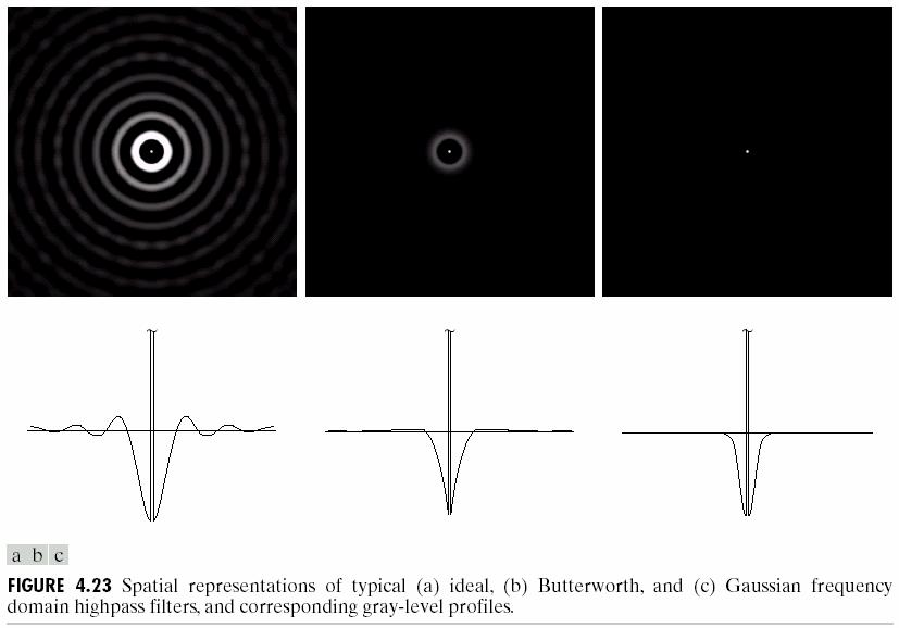
65 Sharpening Frequency Domain Filters Fig shows typical 3-D plots image representations and cross sections for these filters IHPF BHPF GHPF. Fig illustrates what these filters look like in the spatial domain. A spatial representation of a frequency domain filter is obtained by 1multiplying Huv by -1 u+v for centering 2computing the inverse DFT 3 multiplying the real part of the inverse DFT by -1 +y
66
67
68 Sharpening Frequency Domain Filters Ideal Highpass Filters Butterworth Highpass Filters Gaussian Highpass Filters The Laplacian in the Frequency Domain Unsharp Masking High-Boost Filtering and High-Frequency Emphasis Filtering
69 Ideal Highpass Filters A 2-D ideal highpass filter IHPF is defined as 0 H u v 1 D u v D u v > D 0 is the cutoff distance measured. This filter is the opposite of the ideal lowpass filter. if if D D 0 0
70 Ideal Highpass Filters Fig. 4.24a is so severe that it produced distorted thickened object boundaries. Edges on the top three circles do not show well. The result for D 0 80 is more of what a high pass-filtered image should look like. The edges are much cleaner and less distorted and the smaller objects have been filtered properly.
71 Ideal Highpass Filters
72 Sharpening Frequency Domain Filters Ideal Highpass Filters Butterworth Highpass Filters Gaussian Highpass Filters The Laplacian in the Frequency Domain Unsharp Masking High-Boost Filtering and High-Frequency Emphasis Filtering
73 Butterworth Highpass Filters The transfer function of the Butterworth highpass filter BHPF of order n and will cutoff frequency locus at distance D 0 from the origin is given by H u v 1 D 1+ [ D u v 0 n ] 2 High-frequency emphasis: Adding a constant to a highpass filter to preserve the low-frequency components.
74 Butterworth Highpass Filters Fig. 4.25: The boundary is much less distorted than in Fig even for the smallest value of cut off frequency. Since the center spot sizes of the IHPF and the BHPF are similar the performance of the two filters I terms of filtering the smaller objects is comparable. The transition into higher values of cutoff frequencies is much smoother with the BHPF
75 Butterworth Highpass Filters
76 Sharpening Frequency Domain Filters Ideal Highpass Filters Butterworth Highpass Filters Gaussian Highpass Filters The Laplacian in the Frequency Domain Unsharp Masking High-Boost Filtering and High-Frequency Emphasis Filtering
77 Gaussian Highpass Filters The transfer function of the Gaussian Highpass Filters GHPF with cutoff frequency locus at distance D 0 from the origin is given by 2 D u v H u v 1 ep 2 2D 0
78 Gaussian Highpass Filters Fig. 4.26: As epected the results obtained are smoother than with the previous two filters. Even the filtering of the smaller objects and thin bars cleaner with the Gaussian filter.

79 Gaussian Highpass Filters
80 Sharpening Frequency Domain Filters Ideal Highpass Filters Butterworth Highpass Filters Gaussian Highpass Filters The Laplacian in the Frequency Domain Unsharp Masking High-Boost Filtering and High-Frequency Emphasis Filtering
81 Laplacian in the Frequency Domain It can be shown that: I [ 2 f y ] u 2 + v 2 Fuv The Laplacian can be implemented in the frequency domain by using the filter Shift to center H u v u 2 [ u + v M 2 / v N / 2 2 ].
82 Laplacian in the Frequency Domain The laplacian-filtered image in the spatial domain is obtain by computing the inverse Fourier Transform of HuvFuv 2 f y I 1 { [ u M / v N / 2 2 ] F u v}.
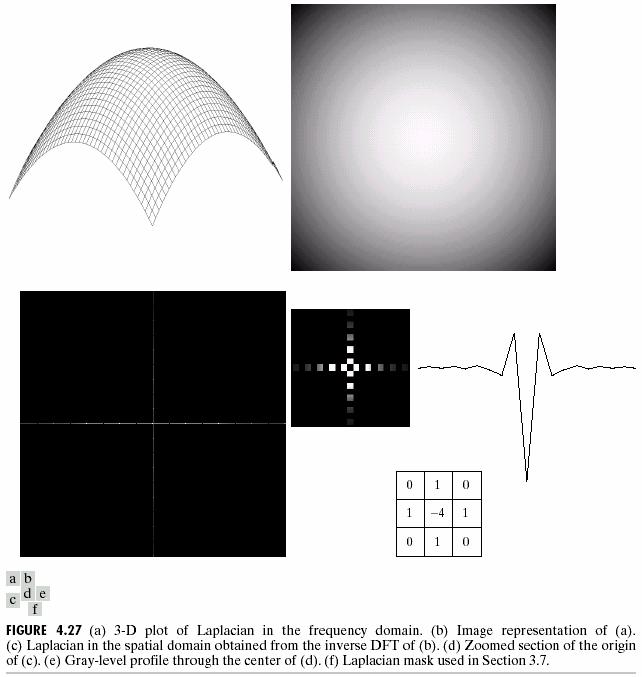
83 Laplacian in the Frequency Domain Fig. 4.27a is a 3-D perspective plot of H u v u 2 + v 2 [ u M / The function is center at M/2N/2 and its value at the top of the dome is zero. All other values are negative. Fig. 4.27b shows Huv as an image also centered. Fig. 4.27c is the Laplacian in the spatial domain v N / 2 2 ].
84
85 Laplacian in the Frequency Domain Fig. 4.28a is the same image in as Fig. 3.40a. Fig. 4.28b shows the result of filtering this image in the frequency domain using f y I { [ u M / 2 + v N / 2 ] F u v}. Fig. 4.28c show the scaled image for display only Fig. 4.28d should be compared with Fig which shows eactly the same sequence of steps but computed using only spatial domain techniques. The results are identical for all practical purposes.

86
87 Sharpening Frequency Domain Filters Ideal Highpass Filters Butterworth Highpass Filters Gaussian Highpass Filters The Laplacian in the Frequency Domain Unsharp Masking High-Boost Filtering and High-Frequency Emphasis Filtering
88 Unsharp Masking High-Boost Filtering Unsharp masking: f hp y fy - f lp y High boost filtering: f hb y Afy - f lp y f hb y A-1fy + f hp y H hb uv A-1 + H hp uv
89 Unsharp Masking High-Boost Filtering Fig b is a highpass filterd iamge. The image in Fig. 4.29c was obtained using f hb y A-1fy + f hp y with A 2. This image is sharper but still too dark. Fig. 4.29d was obtained with A 2.7 which in effect means that the input image was multiplied by 1.7 before the Laplacian was subtracted from it.
90 Unsharp Masking High-Boost Filtering Fig. 4.29d is not as sharp as Fig. 3.43d. The reason for this that a frequency domain representation of the Laplacian is closer to the mask that ecludes the diagonal neighbors [Fig. 4.27f]. It is known that a mask that includes the diagonal neighbors produces slightly sharper results. They do become evident for images with larger features.

91
92 High-Frequency Emphasis Filtering Sometimes it is advantageous to accentuate the contribution to enhancement made by the high-frequency component of an image. We multiply a high pass filter function by a constant and add an offset so that the zero frequency term is not eliminated by the filter. H hfe uv a+bh hp uv where a>0 and b>a. [ Typical a [ ] and b [1.52.0] ]
93 High-Frequency Emphasis Filtering Fig. 4.30a shows a chest X-ray with a narrow range of gray levels. Our objective is to sharpen the image. Fig 4.30c shows image using HFE with a 0.5 and b 2.0. Although the image is still dark the gray level tonality due to the low frequency components was not lost. Fig. 4.30d shows image that is been performing histogram equalization.

94 High-Frequency Emphasis Filtering
95 Background Introduction to the Fourier Transform and the Frequency Domain Smoothing Frequency-Domain Filters Sharpening Frequency Domain Filters Homomorphic Filtering Implementation
96 Homomorphic Filtering We can view an image fy as a product of two components: f 0 0 y i y r y < < i r y y < < iy: illumination. It is determined by the illumination source. ry: reflectance or transmissivity. It is determined by the characteristics of imaged objects. 1
97 Homomorphic Filtering In some images the quality of the image has reduced because of non-uniform illumination. Homomorphic filtering can be used to perform illumination correction. y i y r y f The above equation cannot be used directly in order to operate separately on the frequency components of illumination and reflectance.
98 v u F v u F v u Z r i + y r y i y f y z ln ln ln + ep 0 0 ' ' y r y i y s y g y r y i y s + Homomorphic Filtering v u Z v u H v u S ln : DFT : Huv : DFT -1 : ep :
99 Homomorphic Filtering By separating the illumination and reflectance components homomorphic filter can then operate on them separately. Illumination component of an image generally has slow variations while the reflectance component vary abruptly. By removing the low frequencies highpass filtering the effects of illumination can be removed.
100 Homomorphic Filtering A good idea of control can be gained over the illumination and reflectance components with a homomorphic filter. This control requires specification of a filter function Huv that affects the low and high frequency components of the Fourier transform in different ways. Fig shows a cross section of such a filter. If the parameters γ L and γ H are chosen so that γ L <1and γ H >1. The curve in Fig can be approimated using modified Gaussian highpass filter: H u v 2 γ γ [1 ep c D u v / D ] + γ H L 2 0 L
101 Homomorphic Filtering Fig is typical of the results that can be obtained with the homomorphic filtering function in Fig Fig. 4.33b shows the result of processing this image by homomorphic filtering with γ L 0.5 γ H 2.0 in the filter function of Fig A reduction of dynamic range in the brightness together with an increase in contrast brought out the details of objects inside the shelter and balanced the gray levels of the outside wall. The enhanced image also is sharper.
102 Homomorphic Filtering

103 Homomorphic Filtering
104 Background Introduction to the Fourier Transform and the Frequency Domain Smoothing Frequency-Domain Filters Sharpening Frequency Domain Filters Homomorphic Filtering Implementation
105 Some Additional Properties of the 2-D Fourier Transform Computing the Inverse Fourier Transform Using a Forword Transform Algorithm More on Periodicity: the Need for Padding The Convolution and Correlation Theorems Summary of Properties of the 2-D Fourier Tandform The Fast Fourier Transform Some Comments on Filter Design
106 The Fourier transform pair has the following translation properties: and / / v v u u F e y f N y v M u j + π / / N vy M u j e v u F y y f + π
107 When u 0 M / 2 and v 0 N / 2 it follows that e j 2 0 π u0 / M + v y / N jπ + y e 1 + y In this case Eq becomes f + y y 1 F u M / 2 v N / 2 and similarly f M / 2 y N / 2 F u v 1 u+ v
108 Distributivity snd scaling From the definition of the Fourier transform it follows that And in general that The Fourier transfoem is distributive over addition but nor over multiplication.
109 Distributivity snd scaling For two scalars a and b af y af u v and 1 f a by F / ab u / a v b
110 Rotation If we introduction the polar coordinates r cos θ y r sinθ u ω cosϕ v ω sinϕ Then f y and F u v become f γ θ and F ω ϕ. Direct substitution into definition of the Fourier transform yields f γ θ + θ 0 F ω ϕ + θ 0
111 Periodicity and conjugate symmetry The discrete Fourier transform has the following periodicity properties: The inverse transform also is periodic: N v M u F N v u F v M u F v u F N y M f N y f y M f y f
112 Conjugate symmetry F u v F * u v The spectrum also is symmetric F u v F u v
113 Separability The discrete Fourier transform in Eq can be epressed in the separable form where 1 0 / / / M M u j N y N vy j M M u j e v F M e y f N e M v u F π π π 1 0 / 2 1 N y N vy j e y f N v F π

114
115
116 Some Additional Properties of the 2-D Fourier Transform Computing the Inverse Fourier Transform Using a Forword Transform Algorithm More on Periodicity: the Need for Padding The Convolution and Correlation Theorems Summary of Properties of the 2-D Fourier Tandform The Fast Fourier Transform Some Comments on Filter Design
117 The 1-DFourier transforms: and / 2 1 M M u j e f M u F π 1 0 / 2 M M u j e u F f π
118 Taking the comple conjugate of Eq and dividing both sides by M yields A similar analysis for two variables yields: / / 2 * * 1 1 M u N v N vy M u j e v u F MN y f M π 1 0 / 2 * * 1 1 M u M u j e u F M f M π
119 Some Additional Properties of the 2-D Fourier Transform Computing the Inverse Fourier Transform Using a Forword Transform Algorithm More on Periodicity: the Need for Padding The Convolution and Correlation Theorems Summary of Properties of the 2-D Fourier Tandform The Fast Fourier Transform Some Comments on Filter Design
120 Figure 4.36 illustrates the significance of periodicity. The left column of this figure shows convolution computed using the 1-D version of Eq : * M m m h m f M h f
121
122 This procedure yields etended or padded functions given by and P A A f f e P B B g g e 0 1 0
123
124 Suppose that we have two images fy and hy of sizes A*B and C*D respectively. Wraparound error in 2-D convolution is avoided by choosing: and P A + C 1 Q B + D 1
125 The periodic sequences are formed by etending fy and hy as follows: and Q y B or P A B y and A y f y f e Q y D or P C D y and C y h y h e
126

127
128 Some Additional Properties of the 2-D Fourier Transform Computing the Inverse Fourier Transform Using a Forword Transform Algorithm More on Periodicity: the Need for Padding The Convolution and Correlation Theorems Summary of Properties of the 2-D Fourier Tandform The Fast Fourier Transform Some Comments on Filter Design
129 The discrete convolution of two functions fy and hy of size M*N is denoted by fy*hy and is defined by the epression: The convolution theorem consists of the following relationships between the two functions and their Fourier transforms: and * M m N n n y m h n m f MN y h y f * v u H v u F y h y f * v u H v u F y h y f
130 The correlation of two function fy and hy is defined as: where f* denotes the comple conjugate of f * 1 M m N n n y m h n m f MN y h y f o
131 There is a correlation theorem analogous to the convolution theorem. Let Fuv and Huv denote the Fourier transforms of fy and hy. An analogous result is that correlation in the frequency domain reduces to multiplication in the spatial domain; that is * v u H v u F y h y f o * v u H v u F y h y f o
132 The autocorrelation theorem: f y o f y F u v 2 Similarly f y 2 F u v o F u v

133
134 Some Additional Properties of the 2-D Fourier Transform Computing the Inverse Fourier Transform Using a Forword Transform Algorithm More on Periodicity: the Need for Padding The Convolution and Correlation Theorems Summary of Properties of the 2-D Fourier Tandform The Fast Fourier Transform Some Comments on Filter Design
135
136

137
138
139 Some Additional Properties of the 2-D Fourier Transform Computing the Inverse Fourier Transform Using a Forword Transform Algorithm More on Periodicity: the Need for Padding The Convolution and Correlation Theorems Summary of Properties of the 2-D Fourier Tandform The Fast Fourier Transform Some Comments on Filter Design
140 The FFT algorithm developed in this section is based on the so-called successive doubling method. For notational convenience we epress Eq in the form F u M 1 0 Where And M is assumed to be of the form or n M 2 1 M W M e f j2π / M u W M M 2K
141 Substitution of Eq into Eq yields Using K u K K u K K u K W f K W f K W f K u F u K u K W W K u K u K K u K W W f K W f K u F
142 Defining and F F 1 K 1 u even u f 2 W K K 0 1 K 1 u odd u f W K K u M u Because W M WM and [ ] u F u F u W F u even odd 2K + u+ M W u 2M W 2M 1 2 u [ F u F u W ] F u + K even odd 2K
143 Continuing this argument for any positive integer value of n leads to recursive epressions for the number of multiplications and additions required to implement the FFT: and m n 2m n n 1 n 1 n a n 2a n n 1
144 The computational advantage of the FFT over a direct implementation of the 1-D DFT is defined as 2 M C M M log M 2 M log M 2 n Because it is assumed that M 2 we can epress Eq in terms of n: C n n 2 n
145
146 Some Additional Properties of the 2-D Fourier Transform Computing the Inverse Fourier Transform Using a Forword Transform Algorithm More on Periodicity: the Need for Padding The Convolution and Correlation Theorems Summary of Properties of the 2-D Fourier Tandform The Fast Fourier Transform Some Comments on Filter Design
147 All the filters discussed in this chapter are specified in equation form. In order to use the filters we simply sample the equation for the desired values of uv. This process results in the filter function Huv. In all our eamples this function was multiplied by the DFT of the input image and the inverse DFT was computed. All forward and inverse Fourier transforms in this chapter were computed with an FFT algorithm.
148 The approach to filtering discussed in this chapter is focused strictly on fundamentals the focus being specifically to eplain the effects of filtering in the frequency domain as clearly as possible. We know of no better way to do that than to treat filtering the way we did here. One can view this development as the basis for "prototyping" a filter. In other words given a problem for which we want to find a filter the frequency domain approach is an ideal tool for eperimenting quickly and with full control over filter parameters. Once a filter for a specific application has been found it often is of interest to implement the filter directly in the spatial domain using firmware and/or hardware.
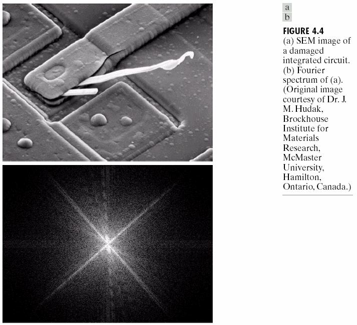
Digital Image Processing. Chapter 4: Image Enhancement in the Frequency Domain
 Digital Image Processing Chapter 4: Image Enhancement in the Frequency Domain Image Enhancement in Frequency Domain Objective: To understand the Fourier Transform and frequency domain and how to apply
Image Enhancement in the frequency domain. GZ Chapter 4
 Image Enhancement in the frequency domain GZ Chapter 4 Contents In this lecture we will look at image enhancement in the frequency domain The Fourier series & the Fourier transform Image Processing in
Digital Image Processing. Filtering in the Frequency Domain
 2D Linear Systems 2D Fourier Transform and its Properties The Basics of Filtering in Frequency Domain Image Smoothing Image Sharpening Selective Filtering Implementation Tips 1 General Definition: System
Digital Image Processing COSC 6380/4393
 Digital Image Processing COSC 6380/4393 Lecture 13 Oct 2 nd, 2018 Pranav Mantini Slides from Dr. Shishir K Shah, and Frank Liu Review f 0 0 0 1 0 0 0 0 w 1 2 3 2 8 Zero Padding 0 0 0 0 0 0 0 1 0 0 0 0
IMAGE ENHANCEMENT: FILTERING IN THE FREQUENCY DOMAIN. Francesca Pizzorni Ferrarese
 IMAGE ENHANCEMENT: FILTERING IN THE FREQUENCY DOMAIN Francesca Pizzorni Ferrarese Contents In this lecture we will look at image enhancement in the frequency domain Jean Baptiste Joseph Fourier The Fourier
Fourier series: Any periodic signals can be viewed as weighted sum. different frequencies. view frequency as an
 Image Enhancement in the Frequency Domain Fourier series: Any periodic signals can be viewed as weighted sum of sinusoidal signals with different frequencies Frequency Domain: view frequency as an independent
Digital Image Processing. Image Enhancement: Filtering in the Frequency Domain
 Digital Image Processing Image Enhancement: Filtering in the Frequency Domain 2 Contents In this lecture we will look at image enhancement in the frequency domain Jean Baptiste Joseph Fourier The Fourier
Filtering in the Frequency Domain
 Filtering in the Frequency Domain Outline Fourier Transform Filtering in Fourier Transform Domain 2/20/2014 2 Fourier Series and Fourier Transform: History Jean Baptiste Joseph Fourier, French mathematician
Chapter 4 Image Enhancement in the Frequency Domain
 Chapter 4 Image Enhancement in the Frequency Domain 3. Fourier transorm -D Let be a unction o real variable,the ourier transorm o is F { } F u ep jπu d j F { F u } F u ep[ jπ u ] du F u R u + ji u or F
Filtering in Frequency Domain
 Dr. Praveen Sankaran Department of ECE NIT Calicut February 4, 2013 Outline 1 2D DFT - Review 2 2D Sampling 2D DFT - Review 2D Impulse Train s [t, z] = m= n= δ [t m T, z n Z] (1) f (t, z) s [t, z] sampled
Convolution Spatial Aliasing Frequency domain filtering fundamentals Applications Image smoothing Image sharpening
 Frequency Domain Filtering Correspondence between Spatial and Frequency Filtering Fourier Transform Brief Introduction Sampling Theory 2 D Discrete Fourier Transform Convolution Spatial Aliasing Frequency
Lecture 4 Filtering in the Frequency Domain. Lin ZHANG, PhD School of Software Engineering Tongji University Spring 2016
 Lecture 4 Filtering in the Frequency Domain Lin ZHANG, PhD School of Software Engineering Tongji University Spring 2016 Outline Background From Fourier series to Fourier transform Properties of the Fourier
Image Enhancement in the frequency domain. Inel 5046 Prof. Vidya Manian
 Image Enhancement in the frequency domain Inel 5046 Prof. Vidya Manian Introduction 2D Fourier transform Basics of filtering in frequency domain Ideal low pass filter Gaussian low pass filter Ideal high
EECS490: Digital Image Processing. Lecture #11
 Lecture #11 Filtering Applications: OCR, scanning Highpass filters Laplacian in the frequency domain Image enhancement using highpass filters Homomorphic filters Bandreject/bandpass/notch filters Correlation
Computer Vision. Filtering in the Frequency Domain
 Computer Vision Filtering in the Frequency Domain Filippo Bergamasco (filippo.bergamasco@unive.it) http://www.dais.unive.it/~bergamasco DAIS, Ca Foscari University of Venice Academic year 2016/2017 Introduction
ECG782: Multidimensional Digital Signal Processing
 Professor Brendan Morris, SEB 3216, brendan.morris@unlv.edu ECG782: Multidimensional Digital Signal Processing Filtering in the Frequency Domain http://www.ee.unlv.edu/~b1morris/ecg782/ 2 Outline Background
Machine vision. Summary # 4. The mask for Laplacian is given
 1 Machine vision Summary # 4 The mask for Laplacian is given L = 0 1 0 1 4 1 (6) 0 1 0 Another Laplacian mask that gives more importance to the center element is L = 1 1 1 1 8 1 (7) 1 1 1 Note that the
Digital Image Processing. Lecture 8 (Enhancement in the Frequency domain) Bu-Ali Sina University Computer Engineering Dep.
 Bu-Ali Sina University Computer Engineering Dep.") Digital Image Processing Lectre 8 Enhancement in the Freqenc domain B-Ali Sina Uniersit Compter Engineering Dep. Fall 009 Image Enhancement In The Freqenc Domain Otline Jean Baptiste Joseph Forier The
Digital Image Processing Lectre 8 Enhancement in the Freqenc domain B-Ali Sina Uniersit Compter Engineering Dep. Fall 009 Image Enhancement In The Freqenc Domain Otline Jean Baptiste Joseph Forier The
Chapter 4: Filtering in the Frequency Domain. Fourier Analysis R. C. Gonzalez & R. E. Woods
 Fourier Analysis 1992 2008 R. C. Gonzalez & R. E. Woods Properties of δ (t) and (x) δ : f t) δ ( t t ) dt = f ( ) f x) δ ( x x ) = f ( ) ( 0 t0 x= ( 0 x0 1992 2008 R. C. Gonzalez & R. E. Woods Sampling
Machine vision, spring 2018 Summary 4
 Machine vision Summary # 4 The mask for Laplacian is given L = 4 (6) Another Laplacian mask that gives more importance to the center element is given by L = 8 (7) Note that the sum of the elements in the
Empirical Mean and Variance!
 Global Image Properties! Global image properties refer to an image as a whole rather than components. Computation of global image properties is often required for image enhancement, preceding image analysis.!
Digital Image Processing
 Digital Image Processing Image Transforms Unitary Transforms and the 2D Discrete Fourier Transform DR TANIA STATHAKI READER (ASSOCIATE PROFFESOR) IN SIGNAL PROCESSING IMPERIAL COLLEGE LONDON What is this
The spatial frequency domain
 The spatial frequenc /3/5 wk9-a- Recall: plane wave propagation λ z= θ path dela increases linearl with E ep i2π sinθ + λ z i2π cosθ λ z plane of observation /3/5 wk9-a-2 Spatial frequenc angle of propagation?
Computer Vision & Digital Image Processing. Periodicity of the Fourier transform
 Computer Vision & Digital Image Processing Fourier Transform Properties, the Laplacian, Convolution and Correlation Dr. D. J. Jackson Lecture 9- Periodicity of the Fourier transform The discrete Fourier
Fourier Transform 2D
 Image Processing - Lesson 8 Fourier Transform 2D Discrete Fourier Transform - 2D Continues Fourier Transform - 2D Fourier Properties Convolution Theorem Eamples = + + + The 2D Discrete Fourier Transform
Review of Linear Systems Theory
 Review of Linear Systems Theory The following is a (very) brief review of linear systems theory, convolution, and Fourier analysis. I work primarily with discrete signals, but each result developed in
Introduction to Computer Vision. 2D Linear Systems
 Introduction to Computer Vision D Linear Systems Review: Linear Systems We define a system as a unit that converts an input function into an output function Independent variable System operator or Transfer
ECE 425. Image Science and Engineering
 ECE 425 Image Science and Engineering Spring Semester 2000 Course Notes Robert A. Schowengerdt schowengerdt@ece.arizona.edu (520) 62-2706 (voice), (520) 62-8076 (fa) ECE402 DEFINITIONS 2 Image science
Signals and Systems. Lecture 11 Wednesday 22 nd November 2017 DR TANIA STATHAKI
 Signals and Systems Lecture 11 Wednesday 22 nd November 2017 DR TANIA STATHAKI READER (ASSOCIATE PROFFESOR) IN SIGNAL PROCESSING IMPERIAL COLLEGE LONDON Effect on poles and zeros on frequency response
Digital Image Processing COSC 6380/4393
 Digital Image Processing COSC 6380/4393 Lecture 11 Oct 3 rd, 2017 Pranav Mantini Slides from Dr. Shishir K Shah, and Frank Liu Review: 2D Discrete Fourier Transform If I is an image of size N then Sin
Lecture Outline. Basics of Spatial Filtering Smoothing Spatial Filters. Sharpening Spatial Filters
 1 Lecture Outline Basics o Spatial Filtering Smoothing Spatial Filters Averaging ilters Order-Statistics ilters Sharpening Spatial Filters Laplacian ilters High-boost ilters Gradient Masks Combining Spatial
Local Enhancement. Local enhancement
 Local Enhancement Local Enhancement Median filtering (see notes/slides, 3.5.2) HW4 due next Wednesday Required Reading: Sections 3.3, 3.4, 3.5, 3.6, 3.7 Local Enhancement 1 Local enhancement Sometimes
G52IVG, School of Computer Science, University of Nottingham
 Image Transforms Fourier Transform Basic idea 1 Image Transforms Fourier transform theory Let f(x) be a continuous function of a real variable x. The Fourier transform of f(x) is F ( u) f ( x)exp[ j2πux]
Chapter 16. Local Operations
 Chapter 16 Local Operations g[x, y] =O{f[x ± x, y ± y]} In many common image processing operations, the output pixel is a weighted combination of the gray values of pixels in the neighborhood of the input
Lecture 4.2 Finite Difference Approximation
 Lecture 4. Finite Difference Approimation 1 Discretization As stated in Lecture 1.0, there are three steps in numerically solving the differential equations. They are: 1. Discretization of the domain by
Optimum Ordering and Pole-Zero Pairing. Optimum Ordering and Pole-Zero Pairing Consider the scaled cascade structure shown below
 Pole-Zero Pairing of the Cascade Form IIR Digital Filter There are many possible cascade realiations of a higher order IIR transfer function obtained by different pole-ero pairings and ordering Each one
Scientific Computing: An Introductory Survey
 Scientific Computing: An Introductory Survey Chapter 12 Prof. Michael T. Heath Department of Computer Science University of Illinois at Urbana-Champaign Copyright c 2002. Reproduction permitted for noncommercial,
CITS 4402 Computer Vision
 CITS 4402 Computer Vision Prof Ajmal Mian Adj/A/Prof Mehdi Ravanbakhsh, CEO at Mapizy (www.mapizy.com) and InFarm (www.infarm.io) Lecture 04 Greyscale Image Analysis Lecture 03 Summary Images as 2-D signals
C. Finding roots of trinomials: 1st Example: x 2 5x = 14 x 2 5x 14 = 0 (x 7)(x + 2) = 0 Answer: x = 7 or x = -2
(x + 2) = 0 Answer: x = 7 or x = -2") AP Calculus Students: Welcome to AP Calculus. Class begins in approimately - months. In this packet, you will find numerous topics that were covered in your Algebra and Pre-Calculus courses. These are
AP Calculus Students: Welcome to AP Calculus. Class begins in approimately - months. In this packet, you will find numerous topics that were covered in your Algebra and Pre-Calculus courses. These are
1-D MATH REVIEW CONTINUOUS 1-D FUNCTIONS. Kronecker delta function and its relatives. x 0 = 0
 -D MATH REVIEW CONTINUOUS -D FUNCTIONS Kronecker delta function and its relatives delta function δ ( 0 ) 0 = 0 NOTE: The delta function s amplitude is infinite and its area is. The amplitude is shown as
IMAGE ENHANCEMENT II (CONVOLUTION)
") MOTIVATION Recorded images often exhibit problems such as: blurry noisy Image enhancement aims to improve visual quality Cosmetic processing Usually empirical techniques, with ad hoc parameters ( whatever
MOTIVATION Recorded images often exhibit problems such as: blurry noisy Image enhancement aims to improve visual quality Cosmetic processing Usually empirical techniques, with ad hoc parameters ( whatever
Local enhancement. Local Enhancement. Local histogram equalized. Histogram equalized. Local Contrast Enhancement. Fig 3.23: Another example
 Local enhancement Local Enhancement Median filtering Local Enhancement Sometimes Local Enhancement is Preferred. Malab: BlkProc operation for block processing. Left: original tire image. 0/07/00 Local
Contents. Signals as functions (1D, 2D)
") Fourier Transform The idea A signal can be interpreted as en electromagnetic wave. This consists of lights of different color, or frequency, that can be split apart usign an optic prism. Each component
Fourier Transform The idea A signal can be interpreted as en electromagnetic wave. This consists of lights of different color, or frequency, that can be split apart usign an optic prism. Each component
ECG782: Multidimensional Digital Signal Processing
 Professor Brendan Morris, SEB 3216, brendan.morris@unlv.edu ECG782: Multidimensional Digital Signal Processing Spring 2014 TTh 14:30-15:45 CBC C313 Lecture 05 Image Processing Basics 13/02/04 http://www.ee.unlv.edu/~b1morris/ecg782/
2. Image Transforms. f (x)exp[ 2 jπ ux]dx (1) F(u)exp[2 jπ ux]du (2)
![2. Image Transforms. f (x)exp[ 2 jπ ux]dx (1) F(u)exp[2 jπ ux]du (2)](/thumbs/73/69504092.jpg "2. Image Transforms. f (x)exp[ 2 jπ ux]dx (1) F(u)exp[2 jπ ux]du (2)") 2. Image Transforms Transform theory plays a key role in image processing and will be applied during image enhancement, restoration etc. as described later in the course. Many image processing algorithms
2. Image Transforms Transform theory plays a key role in image processing and will be applied during image enhancement, restoration etc. as described later in the course. Many image processing algorithms
Midterm Summary Fall 08. Yao Wang Polytechnic University, Brooklyn, NY 11201
 Midterm Summary Fall 8 Yao Wang Polytechnic University, Brooklyn, NY 2 Components in Digital Image Processing Output are images Input Image Color Color image image processing Image Image restoration Image
Key Intuition: invertibility
 Introduction to Fourier Analysis CS 510 Lecture #6 January 30, 2017 In the extreme, a square wave Graphic from http://www.mechatronics.colostate.edu/figures/4-4.jpg 2 Fourier Transform Formally, the Fourier
GBS765 Electron microscopy
 GBS765 Electron microscopy Lecture 1 Waves and Fourier transforms 10/14/14 9:05 AM Some fundamental concepts: Periodicity! If there is some a, for a function f(x), such that f(x) = f(x + na) then function
Contents. Signals as functions (1D, 2D)
") Fourier Transform The idea A signal can be interpreted as en electromagnetic wave. This consists of lights of different color, or frequency, that can be split apart usign an optic prism. Each component
Fourier Transform The idea A signal can be interpreted as en electromagnetic wave. This consists of lights of different color, or frequency, that can be split apart usign an optic prism. Each component
1 1.27z z 2. 1 z H 2
 E481 Digital Signal Processing Exam Date: Thursday -1-1 16:15 18:45 Final Exam - Solutions Dan Ellis 1. (a) In this direct-form II second-order-section filter, the first stage has
Contents. Signals as functions (1D, 2D)
") Fourier Transform The idea A signal can be interpreted as en electromagnetic wave. This consists of lights of different color, or frequency, that can be split apart usign an optic prism. Each component
Fourier Transform The idea A signal can be interpreted as en electromagnetic wave. This consists of lights of different color, or frequency, that can be split apart usign an optic prism. Each component
COMP344 Digital Image Processing Fall 2007 Final Examination
 COMP344 Digital Image Processing Fall 2007 Final Examination Time allowed: 2 hours Name Student ID Email Question 1 Question 2 Question 3 Question 4 Question 5 Question 6 Total With model answer HK University
3. Lecture. Fourier Transformation Sampling
 3. Lecture Fourier Transformation Sampling Some slides taken from Digital Image Processing: An Algorithmic Introduction using Java, Wilhelm Burger and Mark James Burge Separability ² The 2D DFT can be
Image Filtering. Slides, adapted from. Steve Seitz and Rick Szeliski, U.Washington
 Image Filtering Slides, adapted from Steve Seitz and Rick Szeliski, U.Washington The power of blur All is Vanity by Charles Allen Gillbert (1873-1929) Harmon LD & JuleszB (1973) The recognition of faces.
9. Image filtering in the spatial and frequency domains
 Image Processing - Laboratory 9: Image filtering in the spatial and frequency domains 9. Image filtering in the spatial and frequency domains 9.. Introduction In this laboratory the convolution operator
Some commonly encountered sets and their notations
 NATIONAL UNIVERSITY OF SINGAPORE DEPARTMENT OF MATHEMATICS (This notes are based on the book Introductory Mathematics by Ng Wee Seng ) LECTURE SETS & FUNCTIONS Some commonly encountered sets and their
Chapter 4 Imaging. Lecture 21. d (110) Chem 793, Fall 2011, L. Ma
 Chem 793, Fall 2011, L. Ma") Chapter 4 Imaging Lecture 21 d (110) Imaging Imaging in the TEM Diraction Contrast in TEM Image HRTEM (High Resolution Transmission Electron Microscopy) Imaging or phase contrast imaging STEM imaging a
Chapter 4 Imaging Lecture 21 d (110) Imaging Imaging in the TEM Diraction Contrast in TEM Image HRTEM (High Resolution Transmission Electron Microscopy) Imaging or phase contrast imaging STEM imaging a
Announcements. Filtering. Image Filtering. Linear Filters. Example: Smoothing by Averaging. Homework 2 is due Apr 26, 11:59 PM Reading:
 Announcements Filtering Homework 2 is due Apr 26, :59 PM eading: Chapter 4: Linear Filters CSE 52 Lecture 6 mage Filtering nput Output Filter (From Bill Freeman) Example: Smoothing by Averaging Linear
Nonlinear Oscillations and Chaos
 CHAPTER 4 Nonlinear Oscillations and Chaos 4-. l l = l + d s d d l l = l + d m θ m (a) (b) (c) The unetended length of each spring is, as shown in (a). In order to attach the mass m, each spring must be
PSET 0 Due Today by 11:59pm Any issues with submissions, post on Piazza. Fall 2018: T-R: Lopata 101. Median Filter / Order Statistics
 CSE 559A: Computer Vision OFFICE HOURS This Friday (and this Friday only): Zhihao's Office Hours in Jolley 43 instead of 309. Monday Office Hours: 5:30-6:30pm, Collaboration Space @ Jolley 27. PSET 0 Due
Introduction to the Fourier transform. Computer Vision & Digital Image Processing. The Fourier transform (continued) The Fourier transform (continued)
 The Fourier transform (continued)") Introduction to the Fourier transform Computer Vision & Digital Image Processing Fourier Transform Let f(x) be a continuous function of a real variable x The Fourier transform of f(x), denoted by I {f(x)}
Introduction to the Fourier transform Computer Vision & Digital Image Processing Fourier Transform Let f(x) be a continuous function of a real variable x The Fourier transform of f(x), denoted by I {f(x)}
AP Calculus BC Summer Assignment 2018
 AP Calculus BC Summer Assignment 018 Name: When you come back to school, I will epect you to have attempted every problem. These skills are all different tools that we will pull out of our toolbo at different
Statistical Geometry Processing Winter Semester 2011/2012
 Statistical Geometry Processing Winter Semester 2011/2012 Linear Algebra, Function Spaces & Inverse Problems Vector and Function Spaces 3 Vectors vectors are arrows in space classically: 2 or 3 dim. Euclidian
Multidimensional partitions of unity and Gaussian terrains
 and Gaussian terrains Richard A. Bale, Jeff P. Grossman, Gary F. Margrave, and Michael P. Lamoureu ABSTRACT Partitions of unity play an important rôle as amplitude-preserving windows for nonstationary
MIT 2.71/2.710 Optics 10/31/05 wk9-a-1. The spatial frequency domain
 10/31/05 wk9-a-1 The spatial frequency domain Recall: plane wave propagation x path delay increases linearly with x λ z=0 θ E 0 x exp i2π sinθ + λ z i2π cosθ λ z plane of observation 10/31/05 wk9-a-2 Spatial
Fourier Series Representation of
 Fourier Series Representation of Periodic Signals Rui Wang, Assistant professor Dept. of Information and Communication Tongji University it Email: ruiwang@tongji.edu.cn Outline The response of LIT system
Example 1: What do you know about the graph of the function
 Section 1.5 Analyzing of Functions In this section, we ll look briefly at four types of functions: polynomial functions, rational functions, eponential functions and logarithmic functions. Eample 1: What
MATHEMATICS FOR ENGINEERING
 MATHEMATICS FOR ENGINEERING INTEGRATION TUTORIAL FURTHER INTEGRATION This tutorial is essential pre-requisite material for anyone studying mechanical engineering. This tutorial uses the principle of learning
Review of Linear System Theory
 Review of Linear System Theory The following is a (very) brief review of linear system theory and Fourier analysis. I work primarily with discrete signals. I assume the reader is familiar with linear algebra
Exponential and Logarithmic Functions
 Lesson 6 Eponential and Logarithmic Fu tions Lesson 6 Eponential and Logarithmic Functions Eponential functions are of the form y = a where a is a constant greater than zero and not equal to one and is
Image Segmentation: Definition Importance. Digital Image Processing, 2nd ed. Chapter 10 Image Segmentation.
 : Definition Importance Detection of Discontinuities: 9 R = wi z i= 1 i Point Detection: 1. A Mask 2. Thresholding R T Line Detection: A Suitable Mask in desired direction Thresholding Line i : R R, j
AP Calculus AB Summer Assignment
 AP Calculus AB 07-08 Summer Assignment Welcome to AP Calculus AB! You are epected to complete the attached homework assignment during the summer. This is because of class time constraints and the amount
Today s lecture. The Fourier transform. Sampling, aliasing, interpolation The Fast Fourier Transform (FFT) algorithm
 algorithm") Today s lecture The Fourier transform What is it? What is it useful for? What are its properties? Sampling, aliasing, interpolation The Fast Fourier Transform (FFT) algorithm Jean Baptiste Joseph Fourier
Today s lecture The Fourier transform What is it? What is it useful for? What are its properties? Sampling, aliasing, interpolation The Fast Fourier Transform (FFT) algorithm Jean Baptiste Joseph Fourier
Introduction to the Discrete Fourier Transform
 Introduction to the Discrete ourier Transform Lucas J. van Vliet www.ph.tn.tudelft.nl/~lucas TNW: aculty of Applied Sciences IST: Imaging Science and technology PH: Linear Shift Invariant System A discrete
Fourier Analysis Fourier Series C H A P T E R 1 1
 C H A P T E R Fourier Analysis 474 This chapter on Fourier analysis covers three broad areas: Fourier series in Secs...4, more general orthonormal series called Sturm iouville epansions in Secs..5 and.6
Additional Pointers. Introduction to Computer Vision. Convolution. Area operations: Linear filtering
 Additional Pointers Introduction to Computer Vision CS / ECE 181B andout #4 : Available this afternoon Midterm: May 6, 2004 W #2 due tomorrow Ack: Prof. Matthew Turk for the lecture slides. See my ECE
HIGHER SCHOOL CERTIFICATE EXAMINATION MATHEMATICS 4 UNIT (ADDITIONAL) Time allowed Three hours (Plus 5 minutes reading time)
 Time allowed Three hours (Plus 5 minutes reading time)") N E W S O U T H W A L E S HIGHER SCHOOL CERTIFICATE EXAMINATION 996 MATHEMATICS 4 UNIT (ADDITIONAL) Time allowed Three hours (Plus 5 minutes reading time) DIRECTIONS TO CANDIDATES Attempt ALL questions.
N E W S O U T H W A L E S HIGHER SCHOOL CERTIFICATE EXAMINATION 996 MATHEMATICS 4 UNIT (ADDITIONAL) Time allowed Three hours (Plus 5 minutes reading time) DIRECTIONS TO CANDIDATES Attempt ALL questions.
Introduction to Fourier Analysis Part 2. CS 510 Lecture #7 January 31, 2018
 Introduction to Fourier Analysis Part 2 CS 510 Lecture #7 January 31, 2018 OpenCV on CS Dept. Machines 2/4/18 CSU CS 510, Ross Beveridge & Bruce Draper 2 In the extreme, a square wave Graphic from http://www.mechatronics.colostate.edu/figures/4-4.jpg
Digital Image Processing
 Digital Image Processing Part 3: Fourier Transform and Filtering in the Frequency Domain AASS Learning Systems Lab, Dep. Teknik Room T109 (Fr, 11-1 o'clock) achim.lilienthal@oru.se Course Book Chapter
APPM 1360 Final Exam Spring 2016
 APPM 36 Final Eam Spring 6. 8 points) State whether each of the following quantities converge or diverge. Eplain your reasoning. a) The sequence a, a, a 3,... where a n ln8n) lnn + ) n!) b) ln d c) arctan
DISCRETE FOURIER TRANSFORM
 DD2423 Image Processing and Computer Vision DISCRETE FOURIER TRANSFORM Mårten Björkman Computer Vision and Active Perception School of Computer Science and Communication November 1, 2012 1 Terminology:
Lecture 18. Double Integrals (cont d) Electrostatic field near an infinite flat charged plate
 Electrostatic field near an infinite flat charged plate") Lecture 18 ouble Integrals (cont d) Electrostatic field near an infinite flat charged plate Consider a thin, flat plate of infinite size that is charged, with constant charge density ρ (in appropriate
Lecture 18 ouble Integrals (cont d) Electrostatic field near an infinite flat charged plate Consider a thin, flat plate of infinite size that is charged, with constant charge density ρ (in appropriate
ECE 410 DIGITAL SIGNAL PROCESSING D. Munson University of Illinois Chapter 12
 . ECE 40 DIGITAL SIGNAL PROCESSING D. Munson University of Illinois Chapter IIR Filter Design ) Based on Analog Prototype a) Impulse invariant design b) Bilinear transformation ( ) ~ widely used ) Computer-Aided
THE WAVE EQUATION (5.1)
") THE WAVE EQUATION 5.1. Solution to the wave equation in Cartesian coordinates Recall the Helmholtz equation for a scalar field U in rectangular coordinates U U r, ( r, ) r, 0, (5.1) Where is the wavenumber,
THE WAVE EQUATION 5.1. Solution to the wave equation in Cartesian coordinates Recall the Helmholtz equation for a scalar field U in rectangular coordinates U U r, ( r, ) r, 0, (5.1) Where is the wavenumber,
18/10/2017. Image Enhancement in the Spatial Domain: Gray-level transforms. Image Enhancement in the Spatial Domain: Gray-level transforms
 Gray-level transforms Gray-level transforms Generic, possibly nonlinear, pointwise operator (intensity mapping, gray-level transformation): Basic gray-level transformations: Negative: s L 1 r Generic log:
Intensity Transformations and Spatial Filtering: WHICH ONE LOOKS BETTER? Intensity Transformations and Spatial Filtering: WHICH ONE LOOKS BETTER?
 : WHICH ONE LOOKS BETTER? 3.1 : WHICH ONE LOOKS BETTER? 3.2 1 Goal: Image enhancement seeks to improve the visual appearance of an image, or convert it to a form suited for analysis by a human or a machine.
Image Analysis. 3. Fourier Transform
 Image Analysis Image Analysis 3. Fourier Transform Lars Schmidt-Thieme Information Systems and Machine Learning Lab (ISMLL) Institute for Business Economics and Information Systems & Institute for Computer
Polynomial Functions of Higher Degree
 SAMPLE CHAPTER. NOT FOR DISTRIBUTION. 4 Polynomial Functions of Higher Degree Polynomial functions of degree greater than 2 can be used to model data such as the annual temperature fluctuations in Daytona
8-1 Exploring Exponential Models
 8- Eploring Eponential Models Eponential Function A function with the general form, where is a real number, a 0, b > 0 and b. Eample: y = 4() Growth Factor When b >, b is the growth factor Eample: y =
Lecture 7: Edge Detection
 #1 Lecture 7: Edge Detection Saad J Bedros sbedros@umn.edu Review From Last Lecture Definition of an Edge First Order Derivative Approximation as Edge Detector #2 This Lecture Examples of Edge Detection
FFTs in Graphics and Vision. Homogenous Polynomials and Irreducible Representations
 FFTs in Graphics and Vision Homogenous Polynomials and Irreducible Representations 1 Outline The 2π Term in Assignment 1 Homogenous Polynomials Representations of Functions on the Unit-Circle Sub-Representations
Lecture 13: Implementation and Applications of 2D Transforms
 Lecture 13: Implementation and Applications of 2D Transforms Harvey Rhody Chester F. Carlson Center for Imaging Science Rochester Institute of Technology rhody@cis.rit.edu October 25, 2005 Abstract The
Mathematics Extension 2
 0 HIGHER SCHOOL CERTIFICATE EXAMINATION Mathematics Etension General Instructions Reading time 5 minutes Working time hours Write using black or blue pen Black pen is preferred Board-approved calculators
F(u) = f e(t)cos2πutdt + = f e(t)cos2πutdt i f o(t)sin2πutdt = F e(u) + if o(u).
 = f e(t)cos2πutdt + = f e(t)cos2πutdt i f o(t)sin2πutdt = F e(u) + if o(u).") The (Continuous) Fourier Transform Matrix Computations and Virtual Spaces Applications in Signal/Image Processing Niclas Börlin niclas.borlin@cs.umu.se Department of Computing Science, Umeå University,
The (Continuous) Fourier Transform Matrix Computations and Virtual Spaces Applications in Signal/Image Processing Niclas Börlin niclas.borlin@cs.umu.se Department of Computing Science, Umeå University,
MATHEMATICS 200 April 2010 Final Exam Solutions
 MATHEMATICS April Final Eam Solutions. (a) A surface z(, y) is defined by zy y + ln(yz). (i) Compute z, z y (ii) Evaluate z and z y in terms of, y, z. at (, y, z) (,, /). (b) A surface z f(, y) has derivatives
System Identification & Parameter Estimation
 System Identification & Parameter Estimation Wb3: SIPE lecture Correlation functions in time & frequency domain Alfred C. Schouten, Dept. of Biomechanical Engineering (BMechE), Fac. 3mE // Delft University
Finite difference modelling, Fourier analysis, and stability
 Finite difference modelling, Fourier analysis, and stability Peter M. Manning and Gary F. Margrave ABSTRACT This paper uses Fourier analysis to present conclusions about stability and dispersion in finite
MATH TOURNAMENT 2012 PROBLEMS SOLUTIONS
 MATH TOURNAMENT 0 PROBLEMS SOLUTIONS. Consider the eperiment of throwing two 6 sided fair dice, where, the faces are numbered from to 6. What is the probability of the event that the sum of the values
SYLLABUS FOR ENTRANCE EXAMINATION NANYANG TECHNOLOGICAL UNIVERSITY FOR INTERNATIONAL STUDENTS A-LEVEL MATHEMATICS
 SYLLABUS FOR ENTRANCE EXAMINATION NANYANG TECHNOLOGICAL UNIVERSITY FOR INTERNATIONAL STUDENTS A-LEVEL MATHEMATICS STRUCTURE OF EXAMINATION PAPER. There will be one -hour paper consisting of 4 questions..
2D Discrete Fourier Transform (DFT)
") 2D Discrete Fourier Transform (DFT) Outline Circular and linear convolutions 2D DFT 2D DCT Properties Other formulations Examples 2 2D Discrete Fourier Transform Fourier transform of a 2D signal defined
2D Discrete Fourier Transform (DFT) Outline Circular and linear convolutions 2D DFT 2D DCT Properties Other formulations Examples 2 2D Discrete Fourier Transform Fourier transform of a 2D signal defined