Filtering in the Frequency Domain

Transcription

1 Filtering in the Frequency Domain

2 Outline Fourier Transform Filtering in Fourier Transform Domain 2/20/2014 2

3 Fourier Series and Fourier Transform: History Jean Baptiste Joseph Fourier, French mathematician and physicist (03/21/ /16/1830) Orphaned: at nine Egyptian expedition with Napoleon I: 1798 Governor of Lower Egypt Permanent Secretary of the French Academy of Sciences: 1822 Théorie analytique de la chaleur : 1822 (The Analytic Theory of Heat) 2/20/2014 3

4 Fourier Series and Fourier Transform: History Fourier Series Any periodic function can be expressed as the sum of sines and /or cosines of different frequencies, each multiplied by a different coefficients Fourier Transform Any function that is not periodic can be expressed as the integral of sines and /or cosines multiplied by a weighing function 2/20/2014 4

5 Fourier Series: Example 2/20/2014 5

6 Preliminary Concepts j = 1, a complex number C = R + ji the conjugate C* = R - ji 2 2 C = R + I and θ = arctan( I / R) C = C (cosθ + jsin θ) Using Euler's formula, j C = C e θ 2/20/2014 6

7 Fourier Series A function f( t) of a continuous variable t that is periodic with period, T, can be expressed as the sum of sines and cosines multiplied by appropriate coefficients where f() t = n= ce n 2π n j t T 2π n 1 T /2 j t T cn = f ( t) e dt for n = 0, ± 1, ± 2,... T T /2 2/20/2014 7

8 Impulses and the Sifting Property (1) A unit impulse of a continuous variable t located at t=0, denoted δ ( t), defined as if t = 0 δ () t = 0 if t 0 and is constrained also to satisfy the identity δ ( t) dt = 1 The sifting property f () t δ () t dt = f (0) f () t δ ( t t0) dt = f t0 2/20/ ( )

9 Impulses and the Sifting Property (2) A unit impulse of a discrete variable x located at x=0, denoted δ ( x), defined as 1 if x = 0 δ ( x) = 0 if x 0 and is constrained also to satisfy the identity x= δ ( x) = 1 The sifting property x= f( x) δ ( x) = f(0) x= f( x) δ ( x x ) = f( x ) 0 0 2/20/2014 9

10 Impulses and the Sifting Property (3) impulse train s T ( t), s T () t = δ ( t n T) n= 2/20/

11 Fourier Transform: One Continuous Variable The Fourier Transform of a continous function f ( t) j2πµ t F( µ ) { f()} t f() t e dt =I = The Inverse Fourier Transform of F( µ ) 1 2 f( t) { F( )} F( ) e j πµ t d =I µ = µ µ 2/20/

12 Fourier Transform: One Continuous Variable W /2 j2πµ t j2πµ t F( µ ) = f () t e dt = Ae dt W /2 A A = j = j W j2πµ t W /2 jπµ W jπµ W e e e 2πµ W /2 2π sin( πµ W ) = AW ( πµ W ) 2/20/

13 Fourier Transform: Impulses The Fourier transform of a unit impulse located at the origin: j2πµ t F( µ ) = δ() t e dt = e =1 j2πµ 0 The Fourier transform of a unit impulse located at t = t : j2πµ t F( µ ) = δ( t t0) e dt = e j2πµ t 0 =cos(2 πµ t ) jsin (2 πµ t ) /20/

14 Fourier Transform: Impulse Trains Impulse train s T(), t s T() t = δ ( t n T ) The Fourier series: where s () t = c e T n= n= 2π n j t T 2π n 1 T /2 j t T cn = s () T /2 T t e dt T n 2/20/

15 Fourier Transform: Impulse Trains 2πn 2πn 2πn j πµ t j πµ t I e = e e dt = e e dt 2πn 2πn c j 1 T/2 s 1 /2 () t e j t T j t T dt T n = () t e = T t j dt T/2 T δ T T t j t 2 2 T T T / = e = n Tj2 π ( µ T) t n T = e dt = δ ( µ ) T n n I = e du s T() t = c e = 1 2π n j t 2π n 2 ( ) T 1 ( j t ) j πµ δ µ δ µ t T n T= e T n= 2π nt T n= j T e 2/20/

16 Fourier Transform: Impulse Trains Let S( µ ) denote the Fourier transform of the periodic impulse train S ( t) T 1 S( µ ) S T () t e T n= 2π n j t { } T =I =I 2π n 1 j t T = I e T n= 1 n = δ ( µ ) T T n= 2/20/

17 Fourier Transform and Convolution The convolution of two functions is denoted by the operator f() t ht () = f( τ) ht ( τ) dτ I = j2 { () ()} ( τ) ( τ) τ πµ t f t ht f ht d e dt j2πµ t = f ( τ) h( t τ) e dt dτ j2πµτ = f( τ ) H( µ ) e dτ j2πµτ H f e d = ( µ ) ( τ) τ = H( µ ) F( µ ) 2/20/

18 Fourier Transform and Convolution Fourier Transform Pairs f() t ht () H( µ ) F( µ ) f() tht () H( µ ) F( µ ) 2/20/

19 Fourier Transform of Sampled Functions f () t = f() t s () t T = f() t δ ( t n T) n= 2/20/

20 Fourier Transform of Sampled Functions F ( µ ) =I { f () t } =I { f() t s ()} T t = F( µ )? S( µ ) F ( µ ) = F1 ( µ ) S( µ ) = n F( τ ) S( µ τ) dτ S( µ ) = δ ( µ ) 1 T n= T n = F( τ) δ ( µ τ ) dτ T T n= 1 n = F( τδµ ) ( τ ) dτ T T n= 1 n = F( µ ) T T n= 2/20/

21 Question The Fourier transform of the sampled function (shown in the following figure) is 1. Continuous 2. Discrete 2/20/

22 Fourier Transform of Sampled Functions A bandlimited signal is a signal whose Fourier transform is zero above a certain finite frequency. In other words, if the Fourier transform has finite support then the signal is said to be bandlimited. An example of a simple bandlimited signal is a sinusoid of the form, x( t) = sin(2 π ft + θ) 2/20/

23 Fourier Transform of Sampled Functions F ( µ ) = 1 T n= n F( µ ) T µ max µ max Over-sampling 2/20/ T > 2µ max Critically-sampling 1 T = 2µ max under-sampling 1 T < 2µ max

24 Nyquist Shannon sampling theorem We can recover f() tfrom its sampled version if we can isolate a copy of F ( µ ) from the periodic sequence of copies of this function contained in F ( µ ), the transform of the sampled function f () t Sufficient separation is guaranteed if 1 T 2µ Sampling theorem: A continuous, band-limited function can be recovered completely from a set of its samples if the samples are acquired at a rate exceeding twice the highest frequency content of the function > max 2/20/

25 Nyquist Shannon sampling theorem? 2 () ( ) j πµ t f t = F µ e dµ 2/20/

26 Aliasing If a band-limited function is sampled at a rate that is less than twice its highest frequency? The inverse transform will yield a corrupted function. This effect is known as frequency aliasing or simply as aliasing. 2/20/

27 Aliasing 2/20/

28 Aliasing 2/20/

29 Function Reconstruction from Sampled Data F( µ ) = H( µ ) F ( µ ) 1 { F µ } f() t = I ( ) = I 1 { H( µ ) F ( µ )} = ht () f () t [ ] f( t) = f( n T)sinc ( t n T) / n T n= 2/20/

30 The Discrete Fourier Transform (DFT) of One Variable M 1 j2 πµ xm / ( µ ) ( ), µ 0,1,..., 1 F = f xe = M x= 0 1 f x = F µ e x= M M M 1 j2 πµ xm / ( ) ( ), 0,1,2,..., 1 µ = 0 2/20/

31 2-D Impulse and Sifting Property: Continuous The impulse δ( tz, ), δ( tz, ) if t = z = 0 = 0 otherwise and δ ( t, z) dtdz = 1 The sifting property and f (, t z) δ (, t z) dtdz = f (0,0) f (, t z) δ ( t t, z z ) dtdz = f ( t, z ) /20/

32 2-D Impulse and Sifting Property: Discrete The impulse δ( xy, ), δ( xy, ) 1 if x= y = 0 = 0 otherwise The sifting property and x= y= x= y= f( xy, ) δ ( xy, ) = f(0,0) f( x, y) δ ( x x, y y ) = f( x, y ) /20/

33 2-D Fourier Transform: Continuous and j2 π ( µ t+ νz) F( µν, ) = f (, t z) e dtdz j2 π ( µ t+ νz) ftz (, ) = f(, ) e d d µν µ ν 2/20/

34 2-D Fourier Transform: Continuous j2 π ( µ t+ νz) F( µν, ) = f (, t z) e dtdz = T/2 Z/2 T/2 Z/2 Ae j2 π ( µ t+ νz) dtdz sin( πµ T) sin( πνt) = ATZ πµ T πνt 2/20/

35 2-D Sampling and 2-D Sampling Theorem 2 D impulse train: s (, tz) = δ ( t m Tz, n Z) T Z m= n= 2/20/

36 2-D Sampling and 2-D Sampling Theorem Function ftz (, ) is said to be band-limited if its Fourier transform is 0 outside a rectangle established by the intervals [- µ, µ ] and [- ν, ν ], that is max max F( µν, ) = 0 for µ µ and ν ν x max max Two-dimensional sampling theorem: A continuous, band-limited function ftz (, ) can be recovered with no error from a set of its samples if the sampling intervals are 1 1 T< and Z< 2µ 2ν max ma max max 2/20/

37 2-D Sampling and 2-D Sampling Theorem 2/20/

38 Aliasing in Images: Example In an image system, the number of samples is fixed at 96x96 pixels. If we use this system to digitize checkerboard patterns Under-sampling 2/20/

39 Aliasing in Images: Example Re-sampling 2/20/

40 Aliasing in Images: Example Re-sampling 2/20/

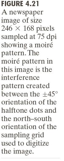
41 Moiré patterns Moiré patterns are often an undesired artifact of images produced by various digital imaging and computer graphics techniques e. g., when scanning a halftone picture or ray tracing a checkered plane. This cause of moiré is a special case of aliasing, due to under-sampling a fine regular pattern 2/20/

42 Moiré patterns 2/20/

43 Moiré patterns A moiré pattern formed by incorrectly downsampling the former image 2/20/

44 Moire Pattern 2/20/

45 2/20/

46 2/20/

47 2-D Discrete Fourier Transform and Its Inverse DFT: M 1N 1 F( µν, ) = f( xye, ) x= 0 y= 0 j2 π ( µ xm / + νyn / ) µ = 0,1,2,..., M 1; ν = 0,1,2,..., N 1; f( xy, ) is a digital image of size M N. IDFT: M 1N 1 1 f( xy, ) = F( µν, ) e MN x= 0 y= 0 j2 π ( µ xm / + νyn / ) 2/20/

48 Properties of the 2-D DFT relationships between spatial and frequency intervals Let T and Z denote the separations between samples, then the seperations between the corresponding discrete, frequency domain variables are given by µ = and ν = 1 M T 1 N Z 2/20/

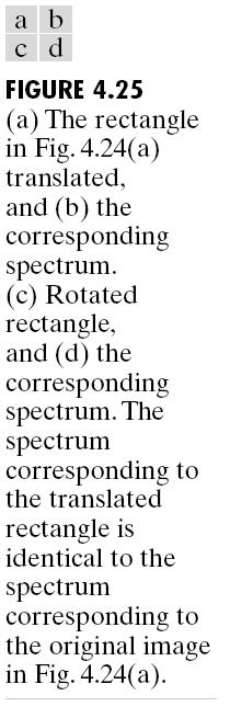
49 Properties of the 2-D DFT translation and rotation and j2 π ( µ 0xM / + ν0yn / ) (, ) (, ) f xye f( x- x, y- y ) F( µν, ) e 0 0 Fµ µ ν ν 0 0 j2 π ( µ x / M+ νy / N) 0 0 Using the polar coordinates x= rcos θ y=rsin θ µ = ωcos ϕ ν= ωsinϕ results in the following transform pair: f(, r θ+ θ) F( ωϕ, + θ) 0 0 2/20/

50 Properties of the 2-D DFT periodicity 2 D Fourier transform and its inverse are infinitely periodic F( µν, ) = F( µ + km, ν ) = F( µν, + k N) = F( µ + km, ν+ k N) f( x, y) = f( x+ k M, y) = f( x, y+ k N) = f( x+ k M, y+ k N) f xe µ µ j 2 π ( µ 0xM ( ) / ) F( ) x µ 0 = M /2, f( x)( 1) F( µ M /2) x+ y f( xy, )( 1) F( µ M/2, ν N/2) 0 2/20/

51 Properties of the 2-D DFT periodicity 2/20/

52 Properties of the 2-D DFT Symmetry 2/20/

53 Properties of the 2-D DFT Fourier Spectrum and Phase Angle 2-D DFT in polar form Fourier spectrum Fuv (, ) = Fuv (, ) e jφ ( uv, ) Fuv = R uv + I uv Power spectrum 2 2 (, ) (, ) (, ) 1/2 Puv = Fuv = R uv + I uv (, ) (, ) (, ) (, ) Phase angle Iuv (, ) φ(u,v)=arctan Ruv (, ) 2/20/

54 2/20/

55 2/20/

56 Example: Phase Angles 2/20/

57 Example: Phase Angles and The Reconstructed 2/20/

58 2-D Convolution Theorem 1-D convolution 2-D convolution M 1 f( x) hx ( ) = f( mhx ) ( m) m= 0 M 1N 1 f( xy, ) hxy (, ) = f( mnhx, ) ( my, n) m= 0 n= 0 x = 0,1,2,..., M 1; y = 0,1,2,..., N 1. f( xy, ) hxy (, ) FuvHuv (, ) (, ) f( xyhxy, ) (, ) Fuv (, ) Huv (, ) 2/20/

59 An Example of Convolution Mirroring h about the origin Translating the mirrored function by x Computing the sum for each x 2/20/

60 An Example of Convolution It causes the wraparoun d error It can be solved by appending zeros 2/20/

61 Zero Padding Consider two functions f(x) and h(x) composed of A and B samples, respectively Append zeros to both functions so that they have the same length, denoted by P, then wraparound is avoided by choosing P A+B-1 2/20/

62 Zero Padding Let f(x,y) and h(x,y) be two image arrays of sizes A B and C D pixels, respectively. Wraparound error in their convolution can be avoided by padding these functions with zeros f h p p ( xy, ) ( xy, ) f ( x, y) 0 x A-1 and 0 y B -1 = 0 A x P or B y Q h( x, y) 0 x C -1 and 0 y D -1 = 0 C x P or D y Q Here P A+ C 1; Q B+ D 1 2/20/

63 Summary 2/20/

64 Summary 2/20/

65 Summary 2/20/

66 Summary 2/20/

67 The Basic Filtering in the Frequency Domain Why is the spectrum at almost ±45 degree stronger than the spectrum at other directions? 2/20/

68 The Basic Filtering in the Frequency Domain Modifying the Fourier transform of an image Computing the inverse transform to obtain the processed result gxy 1 (, ) = I { HuvFuv (, ) (, )} Fuv (, ) is the DFT of the input image Huv (, ) is a filter function. 2/20/

69 The Basic Filtering in the Frequency Domain In a filter H(u,v) that is 0 at the center of the transform and 1 elsewhere, what s the output image? 2/20/

70 The Basic Filtering in the Frequency Domain 2/20/

71 Zero-Phase-Shift Filters gxy = I 1 (, ) { HuvFuv (, ) (, )} Fuv (, ) = Ruv (, ) + jiuv (, ) gxy (, ) =I HuvRuv (, ) (, ) + jhuviuv (, ) (, ) 1 [ ] Filters affect the real and imaginary parts equally, and thus no effect on the phase. These filters are called zero-phase-shift filters 2/20/

72 Examples: Nonzero-Phase-Shift Filters Even small Phase changes angle is in the phase angle Phase angle can is have dramatic multiplied (usually by undesirable) effects multiplied on the by filtered output /20/

73 Summary: Steps for Filtering in the Frequency Domain 1. Given an input image f(x,y) of size MxN, obtain the padding parameters P and Q. Typically, P = 2M and Q = 2N. 2. Form a padded image, f p (x,y) of size PxQ by appending the necessary number of zeros to f(x,y) 3. Multiply f p (x,y) by (-1) x+y to center its transform 4. Compute the DFT, F(u,v) of the image from step 3 5. Generate a real, symmetric filter function*, H(u,v), of size PxQ with center at coordinates (P/2, Q/2) *generate from a given spatial filter, we pad the spatial filter, multiply the expadded array by (-1) x+y, and compute the DFT of the result to obtain a centered H(u,v). 2/20/

74 Summary: Steps for Filtering in the Frequency Domain 6. Form the product G(u,v) = H(u,v)F(u,v) using array multiplication 7. Obtain the processed image { 1 [ ] } (, ) (, ) ( 1) x + g y p x y = real I G u v 8. Obtain the final processed result, g(x,y), by extracting the MxN region from the top, left quadrant of g p (x,y) 2/20/

75 An Example: Steps for Filtering in the Frequency Domain 2/20/

76 Correspondence Between Filtering in the Spatial and Frequency Domains (1) Let H(u) denote the 1-D frequency domain Gaussian filter H ( u) = Ae u /2σ The corresponding filter in the spatial domain h( x) = 2πσ x Ae π σ 1. Both components are Gaussian and real 2. The functions behave reciprocally 2/20/

77 Correspondence Between Filtering in the Spatial and Frequency Domains (2) Let Hu ( ) denote the difference of Gaussian filter /2 σ1 u /2σ2 H ( u) = Ae Be -u - with A B and σ σ 1 2 The corresponding filter in the spatial domain x π σ2 x h( x) = 2πσ Ae 2πσ Ae 2π σ High-pass filter or low-pass filter? 2/20/

78 Correspondence Between Filtering in the Spatial and Frequency Domains (3) 2/20/

79 Correspondence Between Filtering in the Spatial and Frequency Domains: Example 600x600 2/20/

80 Correspondence Between Filtering in the Spatial and Frequency Domains: Example 2/20/

81 Generate H(u,v) f h p p ( xy, ) f ( x, y) 0 x 599 and 0 y 599 = x 602 or 600 y 602 h( x, y) 0 x 2 and 0 y 2 ( xy, ) = 0 3 x 602 or 3 y 602 Here P A(600) + C(3) 1 = 602; Q B(600) + D(3) 1 = /20/

82 Generate H(u,v) x+ y 1. Multiply h( xy, ) by (-1) to center the frequency domain filter p 2. Compute the forward DFT of the result in (1) 3. Set the real part of the resulting DFT to 0 to account for parasitic real parts u+ v 4. Multiply the result by (-1), which is implicit when hxy (, ) was moved to the center of h( xy, ). p 2/20/

83 Image Smoothing Using Filter Domain Filters: ILPF Ideal Lowpass Filters (ILPF) 1 if Duv (, ) Huv (, ) = 0 if Duv (, ) > D D 0 0 D is a positive constant and Duv (, ) is the distance between a point ( uv, ) 0 in the frequency domain and the center of the frequency rectangle Duv (, ) = ( u P/ 2) + ( v Q/ 2) 2 2 1/2 2/20/

84 Image Smoothing Using Filter Domain Filters: ILPF 2/20/

85 ILPF Filtering Example 2/20/

86 ILPF Filtering Example 2/20/

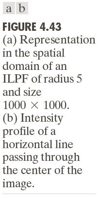
87 The Spatial Representation of ILPF 2/20/

88 Image Smoothing Using Filter Domain Filters: BLPF Butterworth Lowpass Filters (BLPF) of order with cutoff frequency Huv (, ) D 1 = 1 + (, )/ 0 [ Duv D] 0 2n n and 2/20/

89 2/20/

90 The Spatial Representation of BLPF 2/20/

91 Image Smoothing Using Filter Domain Filters: GLPF Gaussian Lowpass Filters (GLPF) in two dimensions is given Huv (, ) = e D 2 2 ( uv, )/2σ By letting σ = D 0 Huv (, ) = e 2 2 (, )/2 0 D uv D 2/20/

92 Image Smoothing Using Filter Domain Filters: GLPF 2/20/

93 2/20/

94 Examples of smoothing by GLPF (1) 2/20/

95 Examples of smoothing by GLPF (2) 2/20/

96 Examples of smoothing by GLPF (3) 2/20/

97 Image Sharpening Using Frequency Domain Filters A highpass filter is obtained from a given lowpass filter using H ( uv, ) = 1 H ( uv, ) HP LP A 2-D ideal highpass filter (IHPL) is defined as 0 if Duv (, ) D Huv (, ) = 1 if Duv (, ) > D 0 0 2/20/

98 Image Sharpening Using Frequency Domain Filters A 2-D Butterworth highpass filter (BHPL) is defined as Huv (, ) 1 = 1 + / (, ) [ D Duv] 2 0 n A 2-D Gaussian highpass filter (GHPL) is defined as Huv (, ) = 1 e 2 2 (, )/2 0 D uv D 2/20/

99 2/20/

100 The Spatial Representation of Highpass Filters 2/20/

101 Filtering Results by IHPF 2/20/

102 Filtering Results by BHPF 2/20/

103 Filtering Results by GHPF 2/20/

104 Using Highpass Filtering and Threshold for Image Enhancement BHPF (order 4 with a cutoff frequency 50) 2/20/

105 The Laplacian in the Frequency Domain Huv = π u + v (, ) 4 ( ) Huv = u P + v Q (, ) 4 π ( / 2) ( / 2) ) = π D ( uv, ) The Laplacian image f( xy, ) =I HuvFuv (, ) (, ) 2 1 { } Enhancement is obtained gxy f xy c f xy c 2 (, ) = (, ) + (, ) = -1 2/20/

106 The Laplacian in the Frequency Domain The enhanced image gxy =I Fuv HuvFuv 1 (, ) (, ) (, ) (, ) 1 =I =I + { } {[ 1 Huv (, )] Fuv (, )} { 1 4 π D( uv, ) Fuv (, )} /20/

107 The Laplacian in the Frequency Domain 2/20/

108 Unsharp Masking, Highboost Filtering and High-Frequency-Emphasis Fitering g ( xy, ) = f( xy, ) f ( xy, ) mask Unsharp masking and highboost filtering gxy (, ) = f( xy, ) + k* g ( xy, ) LP f ( xy, ) = I H ( uvfuv, ) (, ) LP 1 [ ] LP mask [ LP ] [ ] { } gxy =I + k H uv Fuv 1 (, ) 1 * 1 (, ) (, ) 1 =I + { 1 k* H ( uv, ) Fuv (, )} HP 2/20/

109 Unsharp Masking, Highboost Filtering and High-Frequency-Emphasis Fitering {[ ] } gxy (, ) =I k+ k * H ( uv, ) Fuv (, ) k 0 and k HP 2/20/

110 Gaussian Filter D 0 =40 High-Frequency-Emphasis Filtering Gaussian Filter K1=0.5, k2=0.75 2/20/

111 Homomorphic Filtering f( xy, ) = ixyrxy (, ) (, ) [ f( xy, )] [ ixy (, )] [ rxy (, )] I I I =? zxy (, ) = ln f( xy, ) = ln ixy (, ) + ln rxy (, ) { zxy (, )} { ln f( xy, )} { ln ixy (, )} { ln rxy (, )} I =I =I +I Zuv (, ) = F( uv, ) + F( uv, ) i r 2/20/

112 Homomorphic Filtering Suv (, ) = HuvZuv (, ) (, ) sxy = HuvF (, ) ( uv, ) + HuvF (, ) ( uv, ) = I 1 (, ) (, ) { Suv} { HuvF (, ) i( uv, ) HuvF (, ) r( uv, )} { HuvF (, ) ( uv, )} { HuvF (, ) ( uv, )} 1 =I + =I +I 1 1 i = i'( xy, ) + r'( xy, ) i r r gxy e e e i xyr xy (, ) '(, ) '(, ) (, ) = sxy = i xy r xy = 0(, ) 0(, ) 2/20/

113 Homomorphic Filtering The illumination component of an image generally is characterized by slow spatial variations, while the reflectance component tends to vary abruptly These characteristics lead to associating the low frequencies of the Fourier transform of the logarithm of an image with illumination the high frequencies with reflectance. 2/20/

114 Homomorphic Filtering 2 2 c D ( uv, )/ D Huv (,) ( γ γ )1 e 0 = + γ H L L Attenuate the contribution made by illumination and amplify the contribution made by reflectance 2/20/

115 γ L Homomorphic Filtering γ H c = 1 D 0 = = = 80 2/20/

116 Homomorphic Filtering 2/20/

117 Selective Filtering Non-Selective Filters: operate over the entire frequency rectangle Selective Filters operate over some part, not entire frequency rectangle bandreject or bandpass: process specific bands notch filters: process small regions of the frequency rectangle 2/20/

118 Selective Filtering: Bandreject and Bandpass Filters H ( uv, ) = 1 H ( uv, ) BP BR 2/20/

119 Selective Filtering: Bandreject and Bandpass Filters 2/20/

120 Selective Filtering: Notch Filters Zero-phase-shift filters must be symmetric about the origin. A notch with center at (u 0, v 0 ) must have a corresponding notch at location (-u 0,-v 0 ). Notch reject filters are constructed as products of highpass filters whose centers have been translated to the centers of the notches. H ( uv, ) = H( uvh, ) ( uv, ) NR k k k = 1 where H( uv, ) and H ( uv, ) are highpass filters whose centers are k at ( u, v ) and (- u,- v ), respectively. k k k k -k Q 2/20/

121 Selective Filtering: Notch Filters H ( uv, ) = H( uvh, ) ( uv, ) NR k k k = 1 where H( uv, ) and H ( uv, ) are highpass filters whose centers are k at ( u, v ) and (- u,- v ), respectively. k k k k -k A Butterworth notch reject filter of order n H D( uv, ) = ( u M/2 u) + ( v N/2 v) 2 2 k k k D ( uv, ) = ( u M/2 + u) + ( v N/2 + v) Q ( uv, ) = [ D D uv] [ D D uv] NR 2n 2n k = k / k(, ) 1 + 0k / k(, ) 2 2 k k k 2/20/ /2 1/2

122 Examples: Notch Filters (1) A Butterworth notch reject filter D =3 and n=4 for all notch pairs 0 2/20/

123 Examples: Notch Filters (2) 2/20/

124 2/20/