The Mathematics of Deep Learning Part 1: Continuous-time Theory

Transcription

1 The Mathematics of Deep Learning Part 1: Continuous-time Theory Helmut Bőlcskei Department of Information Technology and Electrical Engineering June 2016 joint work with Thomas Wiatowski, Philipp Grohs, and Michael Tschannen

2 Face recognition

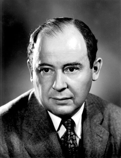
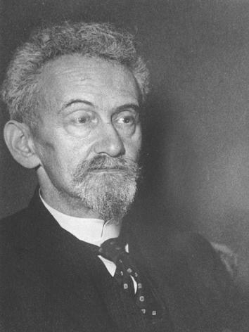
3 Face recognition C. E. Shannon J. von Neumann N. Wiener F. Hausdorff

4 Face recognition C. E. Shannon J. von Neumann N. Wiener F. Hausdorff Feature extraction through deep convolutional neural networks (DCNs)

5 Go! DCNs beat Go-champion Lee Sedol [Silver et al., 2016 ]

6 Atari games DCNs beat professional human Atari-players [Mnih et al., 2015 ]

7 Describing the content of an image DCNs generate sentences describing the content of an image [Vinyals et al., 2015 ]

8 Describing the content of an image DCNs generate sentences describing the content of an image [Vinyals et al., 2015 ] Carlos.

9 Describing the content of an image DCNs generate sentences describing the content of an image [Vinyals et al., 2015 ] Carlos Kleiber.

10 Describing the content of an image DCNs generate sentences describing the content of an image [Vinyals et al., 2015 ] Carlos Kleiber conducting the.

11 Describing the content of an image DCNs generate sentences describing the content of an image [Vinyals et al., 2015 ] Carlos Kleiber conducting the Vienna Philharmonic s.

12 Describing the content of an image DCNs generate sentences describing the content of an image [Vinyals et al., 2015 ] Carlos Kleiber conducting the Vienna Philharmonic s New Year s Concert.

13 Describing the content of an image DCNs generate sentences describing the content of an image [Vinyals et al., 2015 ] Carlos Kleiber conducting the Vienna Philharmonic s New Year s Concert 1989.

14 Feature extraction and learning task DCNs can be used i) as stand-alone feature extractors [Huang and LeCun, 2006 ] input: f = feature extraction R n n feature vector Φ(f) R N learning task output: C. E. Shannon

15 Feature extraction and learning task DCNs can be used i) as stand-alone feature extractors [Huang and LeCun, 2006 ] ii) to perform feature extraction and the learning task directly [LeCun et al., 1990 ] input: f = R n n feature extraction feature vector Φ(f) R N learning task output: C. E. Shannon

16 Why are DCNs so successful? It is the guiding principle of many applied mathematicians that if something mathematical works really well, there must be a good underlying mathematical reason for it, and we ought to be able to understand it. [I. Daubechies, 2015 ]

17 Translation invariance Handwritten digits from the MNIST database [LeCun & Cortes, 1998 ]

18 Translation invariance Handwritten digits from the MNIST database [LeCun & Cortes, 1998 ] Feature vector should be invariant to spatial location translation invariance

19 Deformation insensitivity Handwritten digits from the MNIST database [LeCun & Cortes, 1998 ]

20 Deformation insensitivity Handwritten digits from the MNIST database [LeCun & Cortes, 1998 ] Different handwriting styles correspond to deformations of signals deformation insensitivity

21 Mallat s wavelet-modulus DCN Mallat, 2012, initiated the mathematical analysis of feature extraction through DCNs f ψ λ (k) ψ λ (l) ψ λ (m) f ψ λ (p) ψ λ (r) ψ λ (s) f ψ λ (k) ψ λ (l) f ψ λ (p) ψ λ (r) f ψ λ (k) ψ λ (l) φ J f ψ λ (p) ψ λ (r) φ J f ψ λ (k) f ψ λ (p) f ψ λ (k) φ J f f ψ λ (p) φ J f φ J

22 Mallat s wavelet-modulus DCN Features generated in the n-th network layer Φ n W (f) := { f ψ λ (1) ψ λ (2) ψ λ (n) φ J } λ (1),...,λ (n) Λ W f ψ λ (k) ψ λ (l) ψ λ (m) f ψ λ (p) ψ λ (r) ψ λ (s) f ψ λ (k) ψ λ (l) f ψ λ (p) ψ λ (r) f ψ λ (k) ψ λ (l) φ J f ψ λ (p) ψ λ (r) φ J f ψ λ (k) f ψ λ (p) f ψ λ (k) φ J f f ψ λ (p) φ J f φ J

23 Mallat s wavelet-modulus DCN Directional wavelet system {φ J } {ψ λ } λ ΛW, Λ W := { λ = (j, k) j > J, k {1,..., K} } f φ J 2 2+ λ Λ W f ψ λ 2 2 = f 2 2, f L 2 (R d )

24 Mallat s wavelet-modulus DCN Directional wavelet system {φ J } {ψ λ } λ ΛW, Λ W := { λ = (j, k) j > J, k {1,..., K} } f φ J 2 2+ λ Λ W f ψ λ 2 2 = f 2 2, f L 2 (R d )...and its edge detection capability [Mallat and Zhong, 1992 ] f ψ λ (v) =

25 Mallat s wavelet-modulus DCN Directional wavelet system {φ J } {ψ λ } λ ΛW, Λ W := { λ = (j, k) j > J, k {1,..., K} } f φ J 2 2+ λ Λ W f ψ λ 2 2 = f 2 2, f L 2 (R d )...and its edge detection capability [Mallat and Zhong, 1992 ] f ψ λ (h) =

26 Mallat s wavelet-modulus DCN Directional wavelet system {φ J } {ψ λ } λ ΛW, Λ W := { λ = (j, k) j > J, k {1,..., K} } f φ J 2 2+ λ Λ W f ψ λ 2 2 = f 2 2, f L 2 (R d )...and its edge detection capability [Mallat and Zhong, 1992 ] f ψ λ (d) =

27 Mallat s wavelet-modulus DCN [Mallat, 2012 ] proved that Φ W is horizontally translation-invariant lim Φ W (T t f) Φ W (f) = 0, f L 2 (R d ), t R d, J and stable w.r.t. deformations (F τ f)(x) := f(x τ(x)): Φ W (F τ f) Φ W (f) C ( 2 J τ + J Dτ + D 2 τ ) f W, where W is a wavelet-dependent norm.

28 Mallat s wavelet-modulus DCN [Mallat, 2012 ] proved that Φ W is horizontally translation-invariant lim Φ W (T t f) Φ W (f) = 0, f L 2 (R d ), t R d, J and stable w.r.t. deformations (F τ f)(x) := f(x τ(x)): Φ W (F τ f) Φ W (f) C ( 2 J τ + J Dτ + D 2 τ ) f W, where W is a wavelet-dependent norm. Non-linear deformation (F τ f)(x) = f(x τ(x)):

29 Mallat s wavelet-modulus DCN [Mallat, 2012 ] proved that Φ W is horizontally translation-invariant lim Φ W (T t f) Φ W (f) = 0, f L 2 (R d ), t R d, J and stable w.r.t. deformations (F τ f)(x) := f(x τ(x)): Φ W (F τ f) Φ W (f) C ( 2 J τ + J Dτ + D 2 τ ) f W, where W is a wavelet-dependent norm. Non-linear deformation (F τ f)(x) = f(x τ(x)):

30 Generalizations The basic operations between consecutive layers f f ψ λ (p) ψ λ (q) ψ λ (r) g λ (p) g λ (q) g λ (r) NL NL NL Pool Pool Pool General DCNs employ a wide variety of filters g λ pre-specified and structured (e.g., wavelets [Serre et al., 2005 ]) pre-specified and unstructured (e.g., random filters [Jarrett et al., 2009 ]) learned in a supervised [Huang and LeCun, 2006 ] or an unsupervised [Ranzato et al., 2007 ] fashion

31 Generalizations The basic operations between consecutive layers f f ψ λ (p) ψ λ (q) ψ λ (r) g λ (p) g λ (q) g λ (r) NL NL NL Pool Pool Pool General DCNs employ a wide variety of non-linearities modulus [Mutch and Lowe, 2006 ] hyperbolic tangent [Huang and LeCun, 2006 ] rectified linear unit [Nair and Hinton, 2010 ] logistic sigmoid [Glorot and Bengio, 2010 ]

32 Generalizations The basic operations between consecutive layers f f ψ λ (p) ψ λ (q) ψ λ (r) g λ (p) g λ (q) g λ (r) NL NL NL Pool Pool Pool General DCNs employ intra-layer pooling sub-sampling [Pinto et al., 2008 ] average pooling [Jarrett et al., 2009 ] max-pooling [Ranzato et al., 2007 ]

33 Generalizations The basic operations between consecutive layers f f ψ λ (p) ψ λ (q) ψ λ (r) g λ (p) g λ (q) g λ (r) NL NL NL Pool Pool Pool General DCNs employ different filters, non-linearities, and pooling operations in different network layers [LeCun et al., 2015 ]

34 Generalizations The basic operations between consecutive layers f f ψ λ (p) ψ λ (q) ψ λ (r) g λ (p) g λ (q) g λ (r) NL NL NL Pool Pool Pool φ J φ J φ J χ χ χ General DCNs employ various output filters [He et al., 2015 ]

35 General filters: Semi-discrete frames Observation: Convolutions yield semi-discrete frame coefficients (f g λ )(b) = f, g λ (b ) = f, T b Ig λ, (λ, b) Λ R d

36 General filters: Semi-discrete frames Observation: Convolutions yield semi-discrete frame coefficients Definition (f g λ )(b) = f, g λ (b ) = f, T b Ig λ, (λ, b) Λ R d Let {g λ } λ Λ L 1 (R d ) L 2 (R d ) be indexed by a countable set Λ. The collection Ψ Λ := { T b Ig λ }(λ,b) Λ R d is a semi-discrete frame for L 2 (R d ), if there exist constants A, B > 0 such that A f 2 2 f, T b Ig λ 2 db = f g λ 2 2 B f 2 2, λ Λ R d λ Λ for all f L 2 (R d ).

37 General filters: Semi-discrete frames A f 2 2 λ Λ R d f, T b Ig λ 2 db = λ Λ f g λ 2 2 B f 2 2 Semi-discrete frames are rooted in continuous frame theory [Antoine et al., 1993 ], [Kaiser, 1994 ]

38 General filters: Semi-discrete frames A f 2 2 λ Λ R d f, T b Ig λ 2 db = λ Λ f g λ 2 2 B f 2 2 Semi-discrete frames are rooted in continuous frame theory [Antoine et al., 1993 ], [Kaiser, 1994 ] Sampling the translation parameter b R d in (T b Ig λ ) on Z d leads to shift-invariant frames [Ron and Shen, 1995 ]

39 General filters: Semi-discrete frames A f 2 2 λ Λ R d f, T b Ig λ 2 db = λ Λ f g λ 2 2 B f 2 2 Semi-discrete frames are rooted in continuous frame theory [Antoine et al., 1993 ], [Kaiser, 1994 ] Sampling the translation parameter b R d in (T b Ig λ ) on Z d leads to shift-invariant frames [Ron and Shen, 1995 ] The frame condition can equivalently be expressed as A ĝ λ (ω) 2 B, a.e. ω R d λ Λ

40 General filters: Semi-discrete frames A f 2 2 λ Λ R d f, T b Ig λ 2 db = λ Λ f g λ 2 2 B f 2 2 Semi-discrete frames are rooted in continuous frame theory [Antoine et al., 1993 ], [Kaiser, 1994 ] Sampling the translation parameter b R d in (T b Ig λ ) on Z d leads to shift-invariant frames [Ron and Shen, 1995 ] The frame condition can equivalently be expressed as A λ Λ ĝ λ (ω) 2 B, a.e. ω R d Structured semi-discrete frames: Weyl-Heisenberg frames, wavelets, (α)-curvelets, shearlets, and ridgelets

41 General filters: Semi-discrete frames A f 2 2 λ Λ R d f, T b Ig λ 2 db = λ Λ f g λ 2 2 B f 2 2 Semi-discrete frames are rooted in continuous frame theory [Antoine et al., 1993 ], [Kaiser, 1994 ] Sampling the translation parameter b R d in (T b Ig λ ) on Z d leads to shift-invariant frames [Ron and Shen, 1995 ] The frame condition can equivalently be expressed as A λ Λ ĝ λ (ω) 2 B, a.e. ω R d Structured semi-discrete frames: Weyl-Heisenberg frames, wavelets, (α)-curvelets, shearlets, and ridgelets Λ is typically a collection of scales, directions, or frequency shifts

42 General non-linearities Observation: Essentially all non-linearities M : L 2 (R d ) L 2 (R d ) employed in the deep learning literature are i) pointwise, i.e., for some ρ : C C, ii) Lipschitz-continuous, i.e., (Mf)(x) = ρ(f(x)), x R d, M(f) M(h) L f h, f, h, L 2 (R d ), for some L > 0, iii) satisfy M(f) = 0 for f = 0.

43 Incorporating pooling by sub-sampling Pooling by sub-sampling can be emulated in continuous-time by the (unitary) dilation operator f R d/2 f(r ), f L 2 (R d ), where R 1 is the sub-sampling factor.

44 Different modules in different layers Module-sequence Ω = ( (Ψ n, M n, R n ) ) n N i) in the n-th network layer, replace the wavelet-modulus convolution operation f ψ λ by U n [λ n ]f := Rn d/2 (M n (f g λn ))(R n )

45 Different modules in different layers Module-sequence Ω = ( (Ψ n, M n, R n ) ) n N i) in the n-th network layer, replace the wavelet-modulus convolution operation f ψ λ by U n [λ n ]f := Rn d/2 (M n (f g λn ))(R n ) ii) extend the operator U n [λ n ] to paths on index sets q = (λ 1, λ 2,..., λ n ) Λ 1 Λ 2 Λ n := Λ n 1, n N, according to U[q]f := U n [λ n ] U 2 [λ 2 ]U 1 [λ 1 ]f

46 Output filters [Mallat, 2012 ] employed the same low-pass filter φ J in every network layer n to generate the output according to Φ n W (f) := { f ψ λ (1) ψ λ (2) ψ λ (n) φ J } λ (1),...,λ (n) Λ W

47 Output filters [Mallat, 2012 ] employed the same low-pass filter φ J in every network layer n to generate the output according to Φ n W (f) := { f ψ λ (1) ψ λ (2) ψ λ (n) φ J } λ (1),...,λ (n) Λ W Here, designate one of the atoms {g λn } λn Λn as the outputgenerating atom χ n 1 := g λ n, λ n Λ n, of the (n 1)-th layer. The atoms {g λn } λn Λ n\{λ n } {χ n 1 } are used across two consecutive layers!

48 Generalized feature extractor Features generated in the n-th network layer Φ n Ω(f) := { (U[q]f) χ n } q Λ n 1 U [( λ (j) 1, λ(l) 2, )] λ(m) 3 f U [( λ (p) 1, λ(r) 2, )] λ(s) 3 f U [( λ (j) 1, )] λ(l) 2 f U [( λ (p) 1, )] λ(r) 2 f ( [( (j) U λ 1, )] ) λ(l) 2 f χ2 ( [ (j)] ) U λ 1 f χ1 U [ λ (j) ] 1 f U[e]f = f U [ λ (p) ] 1 f ( [( (p) U λ 1, )] ) λ(r) 2 f χ2 ( [ (p)] ) U λ 1 f χ1 f χ 0

49 Generalized feature extractor Features generated in the n-th network layer Φ n Ω(f) := { (U[q]f) χ n } q Λ n 1 U [( λ (j) 1, λ(l) 2, )] λ(m) 3 f U [( λ (p) 1, λ(r) 2, )] λ(s) 3 f U [( λ (j) 1, )] λ(l) 2 f U [( λ (p) 1, )] λ(r) 2 f ( [( (j) U λ 1, )] ) λ(l) 2 f χ2 ( [( (p) U λ 1, )] ) λ(r) 2 f χ2 U [ λ (j) ] 1 f U [ λ (p) ] 1 f Ψ 2 ( [ (j)] ) U λ 1 f χ1 U[e]f = f ( [ (p)] ) U λ 1 f χ1 f χ 0

50 Vertical translation invariance Theorem (Wiatowski and HB, 2015) Assume that Ω = ( (Ψ n, M n, R n ) ) satisfies the admissibility n N condition B n min{1, L 2 n }, for all n N. If there exists a constant K > 0 such that then χ n (ω) ω K, a.e. ω R d, n N 0, Φ n Ω(T t f) Φ n Ω(f) for all f L 2 (R d ), t R d, n N. 2π t K R 1... R n f 2,

51 Vertical translation invariance The admissibility condition B n min{1, L 2 n }, n N, is easily satisfied by normalizing Ψ n.

52 Vertical translation invariance The admissibility condition B n min{1, L 2 n }, n N, is easily satisfied by normalizing Ψ n. The decay condition χ n (ω) ω K, a.e. ω R d, n N 0, is satisfied, e.g., if sup n N0 { χ n 1 + χ n 1 } <.

53 Vertical translation invariance The admissibility condition B n min{1, L 2 n }, n N, is easily satisfied by normalizing Ψ n. The decay condition χ n (ω) ω K, a.e. ω R d, n N 0, is satisfied, e.g., if sup n N0 { χ n 1 + χ n 1 } <. If, in addition, lim n R 1 R 2... R n =, then lim n Φn Ω(T t f) Φ n Ω(f) = 0, f L 2 (R d ), t R d.

54 Philosophy behind invariance results Mallat s horizontal translation invariance: lim Φ W (T t f) Φ W (f) = 0, J f L 2 (R d ), t R d Vertical translation invariance: lim n Φn Ω(T t f) Φ n Ω(f) = 0, f L 2 (R d ), t R d

55 Philosophy behind invariance results Mallat s horizontal translation invariance: lim Φ W (T t f) Φ W (f) = 0, J f L 2 (R d ), t R d features become invariant in every network layer, but needs J Vertical translation invariance: lim n Φn Ω(T t f) Φ n Ω(f) = 0, f L 2 (R d ), t R d features become more invariant with increasing network depth

56 Philosophy behind invariance results Mallat s horizontal translation invariance: lim Φ W (T t f) Φ W (f) = 0, J f L 2 (R d ), t R d features become invariant in every network layer, but needs J applies to wavelet transform and modulus non-linearity without pooling Vertical translation invariance: lim n Φn Ω(T t f) Φ n Ω(f) = 0, f L 2 (R d ), t R d features become more invariant with increasing network depth applies to general filters, general non-linearities, and pooling through sub-sampling

57 Deformation sensitivity bounds [Mallat, 2012 ] proved that Φ W is stable w.r.t. non-linear deformations (F τ f)(x) = f(x τ(x)) according to Φ W (F τ f) Φ W (f) C ( 2 J τ + J Dτ + D 2 τ ) f W, where H W := { f L 2 (R d ) f W < } with f W := ( n=0 q (Λ W ) n 1 U[q] 2 2 ) 1/2

58 Deformation sensitivity for signal classes Consider (F τ f)(x) = f(x τ(x)) = f(x e x2 ) f 1(x), (F τ f 1)(x) x f 2(x), (F τ f 2)(x) x For given τ the amount of deformation induced can depend drastically on f L 2 (R d )

59 Deformation sensitivity bounds: Band-limited signals Theorem (Wiatowski and HB, 2015) Assume that Ω = ( (Ψ n, M n, R n ) ) satisfies the admissibility n N condition B n min{1, L 2 n }, for all n N. There exists a constant C > 0 (that does not depend on Ω) such that for all f {f L 2 (R d ) supp( ˆf) B R (0)} and all τ C 1 (R d, R d ) with Dτ 1 2d, it holds that Φ Ω (F τ f) Φ Ω (f) CR τ f 2.

60 Deformation sensitivity bounds: Cartoon functions... and what about non-band-limited signals? Image credit: middle [Mnih et al., 2015 ], right [Silver et al., 2016 ]

61 Deformation sensitivity bounds: Cartoon functions... and what about non-band-limited signals? Image credit: middle [Mnih et al., 2015 ], right [Silver et al., 2016 ] Take into account structural properties of natural images. consider cartoon functions [Donoho, 2001 ]

62 Deformation sensitivity bounds: Cartoon functions... and what about non-band-limited signals? Image credit: middle [Mnih et al., 2015 ], right [Silver et al., 2016 ] The class of cartoon functions of maximal size K > 0: C K CART := {f B f 2 f i L 2 (R d ) C 1 (R d, C), i = 1, 2, f i (x) K(1 + x 2 ) d/2, vol d 1 ( B) K, f 2 K}

63 Deformation sensitivity bounds: Cartoon functions Theorem (Grohs et al., 2016) Assume that Ω = ( (Ψ n, M n, R n ) ) satisfies the admissibility n N condition B n min{1, L 2 n }, for all n N. For every K > 0 there exists a constant C K > 0 (that does not depend on Ω) such that for all f CCART K and all τ C1 (R d, R d ) with τ < 1 2 and Dτ 1 2d, it holds that Φ Ω (F τ f) Φ Ω (f) C K τ 1/2.

64 Deformation sensitivity bounds: Lipschitz functions Cartoon functions reduce to Lipschitz functions upon setting f 2 = 0 in f B f 2 C K CART Corollary (Grohs et al., 2016) Assume that Ω = ( (Ψ n, M n, R n ) ) satisfies the admissibility n N condition B n min{1, L 2 n }, for all n N. For every K > 0 there exists a constant C K > 0 (that does not depend on Ω) such that for all f {f L 2 (R d ) f Lipschitz-continuous, f i (x) K(1+ x 2 ) d/2} and all τ C 1 (R d, R d ) with τ < 1 2 and Dτ 1 2d, it holds that Φ Ω (F τ f) Φ Ω (f) C K τ.

65 ... and what about textures?

66 ... and what about textures? neither band-limited, nor a cartoon function, nor Lipschitz-continuous

67 Philosophy behind deformation stability/sensitivity bounds Mallat s deformation stability bound: Φ W (F τ f) Φ W (f) C ( 2 J τ +J Dτ + D 2 τ ) f W, for all f H W L 2 (R d ) The signal class H W and the corresponding norm W depend on the mother wavelet (and hence the network) Our deformation sensitivity bound: Φ Ω (F τ f) Φ Ω (f) C C τ α, f C L 2 (R d ) The signal class C (band-limited functions or cartoon functions) is independent of the network

68 Philosophy behind deformation stability/sensitivity bounds Mallat s deformation stability bound: Φ W (F τ f) Φ W (f) C ( 2 J τ +J Dτ + D 2 τ ) f W, for all f H W L 2 (R d ) Signal class description complexity implicit via norm W Our deformation sensitivity bound: Φ Ω (F τ f) Φ Ω (f) C C τ α, f C L 2 (R d ) Signal class description complexity explicit via C C R-band-limited functions: C C = O(R) cartoon functions of maximal size K: C C = O(K 3/2 ) K-Lipschitz functions C C = O(K)

69 Philosophy behind deformation stability/sensitivity bounds Mallat s deformation stability bound: Φ W (F τ f) Φ W (f) C ( 2 J τ +J Dτ + D 2 τ ) f W, for all f H W L 2 (R d ) Our deformation sensitivity bound: Φ Ω (F τ f) Φ Ω (f) C C τ α, f C L 2 (R d ) Decay rate α > 0 of the deformation error is signal-classspecific (band-limited functions: α = 1, cartoon functions: α = 1 2, Lipschitz functions: α = 1)

70 Philosophy behind deformation stability/sensitivity bounds Mallat s deformation stability bound: Φ W (F τ f) Φ W (f) C ( 2 J τ +J Dτ + D 2 ) τ f W, for all f H W L 2 (R d ) The bound depends explicitly on higher order derivatives of τ Our deformation sensitivity bound: Φ Ω (F τ f) Φ Ω (f) C C τ α, f C L 2 (R d ) The bound implicitly depends on derivatives of τ via the condition Dτ 1 2d

71 Philosophy behind deformation stability/sensitivity bounds Mallat s deformation stability bound: Φ W (F τ f) Φ W (f) C ( 2 J τ +J Dτ + D 2 τ ) f W, for all f H W L 2 (R d ) The bound is coupled to horizontal translation invariance lim Φ W (T t f) Φ W (f) = 0, J Our deformation sensitivity bound: f L 2 (R d ), t R d Φ Ω (F τ f) Φ Ω (f) C C τ α, f C L 2 (R d ) The bound is decoupled from vertical translation invariance lim n Φn Ω(T t f) Φ n Ω(f) = 0, f L 2 (R d ), t R d

72 Proof sketch: Decoupling Φ Ω (F τ f) Φ Ω (f) C C τ α, f C L 2 (R d ) 1) Lipschitz continuity: Φ Ω (f) Φ Ω (h) f h 2, f, h L 2 (R d ), established through (i) frame property of Ψ n, (ii) Lipschitz continuity of non-linearities, and (iii) admissibility condition B n min{1, L 2 n }

73 Proof sketch: Decoupling Φ Ω (F τ f) Φ Ω (f) C C τ α, f C L 2 (R d ) 1) Lipschitz continuity: Φ Ω (f) Φ Ω (h) f h 2, f, h L 2 (R d ), established through (i) frame property of Ψ n, (ii) Lipschitz continuity of non-linearities, and (iii) admissibility condition B n min{1, L 2 n } 2) Signal-class-specific deformation sensitivity bound: F τ f f 2 C C τ α, f C L 2 (R d )

74 Proof sketch: Decoupling Φ Ω (F τ f) Φ Ω (f) C C τ α, f C L 2 (R d ) 1) Lipschitz continuity: Φ Ω (f) Φ Ω (h) f h 2, f, h L 2 (R d ), established through (i) frame property of Ψ n, (ii) Lipschitz continuity of non-linearities, and (iii) admissibility condition B n min{1, L 2 n } 2) Signal-class-specific deformation sensitivity bound: F τ f f 2 C C τ α, f C L 2 (R d ) 3) Combine 1) and 2) to get Φ Ω (F τ f) Φ Ω (f) F τ f f 2 C C τ α, for all f C L 2 (R d )

75 Noise robustness Lipschitz continuity of Φ Ω according to Φ Ω (f) Φ Ω (h) f h 2, f, h L 2 (R d ), also implies robustness w.r.t. additive noise η L 2 (R d ) according to Φ Ω (f + η) Φ Ω (f) η 2

76 Energy conservation It is desirable to have f 0 Φ(f) 0, or even better Φ(f) A Φ f 2, f L 2 (R d ), for some A Φ > 0.

77 Energy conservation It is desirable to have f 0 Φ(f) 0, or even better Φ(f) A Φ f 2, f L 2 (R d ), for some A Φ > 0. [Waldspurger, 2015 ] proved under analyticity assumptions on the mother wavelet that for real-valued signals f L 2 (R d ), Φ W conserves energy according to Φ W (f) = f 2

78 Energy conservation Theorem (Grohs et al., 2016) Let Ω = ( (Ψ n,, 1) ) be a module-sequence employing modulus n N non-linearities and no sub-sampling. For every n N, let the atoms of Ψ n satisfy the following conditions: i) λ n Λ n\{λ n } ĝ λ n (ω) 2 + χ n 1 (ω) 2 = 1, a.e. ω R d ii) λ n Λ n\{λ n } ĝ λ n (ω) 2 = 0, a.e. ω B δn (0), for some δ n > 0 iii) all atoms g λn Then, are analytic. Φ Ω (f) = f 2, f L 2 (R d )

79 Energy conservation Theorem (Grohs et al., 2016) Let Ω = ( (Ψ n,, 1) ) be a module-sequence employing modulus n N non-linearities and no sub-sampling. For every n N, let the atoms of Ψ n satisfy the following conditions: i) λ n Λ n\{λ n } ĝ λ n (ω) 2 + χ n 1 (ω) 2 = 1, a.e. ω R d ii) λ n Λ n\{λ n } ĝ λ n (ω) 2 = 0, a.e. ω B δn (0), for some δ n > 0 iii) all atoms g λn Then, are analytic. Φ Ω (f) = f 2, f L 2 (R d ) Various structured frames satisfy conditions i)-iii)

80 Proof sketch: Energy conservation or What does the modulus non-linearity do? f(ω) ω χ ĝ λ

81 Proof sketch: Energy conservation or What does the modulus non-linearity do? f(ω) ω χ ĝ λ ( f ĝ λ )(ω) ω

82 Proof sketch: Energy conservation or What does the modulus non-linearity do? f(ω) ω χ ĝ λ ( f ĝ λ )(ω) R f ĝλ (ω) ω ω (f g λ )(x) 2 R f ĝλ (ω)

83 Proof sketch: Energy conservation or What does the modulus non-linearity do? f(ω) ω χ ĝ λ ( f ĝ λ )(ω) R f ĝλ (ω) ω χ ω f g λ 2 χ =

84 Two Meta Theorems Meta Theorem Vertical translation invariance and Lipschitz continuity (hence by decoupling also deformation insensitivity) are guaranteed by the network structure per se rather than the specific convolution kernels, non-linearities, and pooling operations.

85 Two Meta Theorems Meta Theorem Vertical translation invariance and Lipschitz continuity (hence by decoupling also deformation insensitivity) are guaranteed by the network structure per se rather than the specific convolution kernels, non-linearities, and pooling operations. Meta Theorem For networks employing the modulus non-linearity and no intra-layer pooling, energy conservation is guaranteed for quite general convolution kernels.

86 Deep Frame Net Open source software: MATLAB: Python: Coming soon!

87 The Mathematics of Deep Learning Part 2: Discrete-time Theory Helmut Bőlcskei Department of Information Technology and Electrical Engineering June 2016 joint work with Thomas Wiatowski, Michael Tschannen, and Philipp Grohs

88 Continuous-time theory [Mallat, 2012 ] and [Wiatowski and HB, 2015 ] developed a continuous-time theory for feature extraction through DCNs: translation invariance results for L 2 (R d )-functions deformation sensitivity bounds for signal classes C L 2 (R d ) energy conservation for L 2 (R d )-functions

89 Practice is digital In practice... we need to handle discrete data! f = R n n

90 Practice is digital In practice... a wide variety of network architectures is used! class probabilities [LeCun et al., 1990 ] f g 1 h 1 f g n h m f g 1 f g n f

91 Practice is digital In practice... a wide variety of network architectures is used! f g 1 h 1 k 1 f g m h n k p f g 1 h 1 f g m h n f g 1 h 1 µ f g m h n µ f g 1 f g m f g 1 f f g m f ϕ low

92 Architecture of general DCNs The basic operations between consecutive layers f g 1 g 2 g n NL NL NL Pool Pool Pool DCNs employ a wide variety of filters g k pre-specified and structured (e.g., wavelets [Serre et al., 2005 ]) pre-specified and unstructured (e.g., random filters [Jarrett et al., 2009 ]) learned in a supervised [Huang and LeCun, 2006 ] or an unsupervised [Ranzato et al., 2007 ] fashion

93 Architecture of general DCNs The basic operations between consecutive layers f g 1 g 2 g n NL NL NL Pool Pool Pool DCNs employ a wide variety of non-linearities modulus [Mutch and Lowe, 2006 ] hyperbolic tangent [Huang and LeCun, 2006 ] rectified linear unit [Nair and Hinton, 2010 ] logistic sigmoid [Glorot and Bengio, 2010 ]

94 Architecture of general DCNs The basic operations between consecutive layers f g 1 g 2 g n NL NL NL Pool Pool Pool DCNs employ pooling sub-sampling [Pinto et al., 2008 ] average pooling [Jarrett et al., 2009 ] max-pooling [Ranzato et al., 2007 ]

95 Architecture of general DCNs The basic operations between consecutive layers f g 1 g 2 g n NL NL NL Pool Pool Pool DCNs employ different filters, non-linearities, and pooling operations in different network layers [LeCun et al., 2015 ]

96 Architecture of general DCNs f g 1 g 2 g n NL NL NL Pool Pool Pool χ χ χ Which layers contribute to the network s output? the last layer only (e.g., class probabilities [LeCun et al., 1990 ]) subset of layers (e.g., shortcut connections [He et al., 2015 ]) all layers (e.g., low-pass filtering [Bruna and Mallat, 2013 ])

97 Challenges Challenges for discrete theory: flexible architectures

98 Challenges Challenges for discrete theory: flexible architectures signals of varying dimensions are propagated through the network

99 Challenges Challenges for discrete theory: flexible architectures signals of varying dimensions are propagated through the network how to incorporate general pooling operators into the theory?

100 Challenges Challenges for discrete theory: flexible architectures signals of varying dimensions are propagated through the network how to incorporate general pooling operators into the theory? can not rely on asymptotics (finite network depth) to prove network properties (e.g., translation invariance)

101 Challenges Challenges for discrete theory: flexible architectures signals of varying dimensions are propagated through the network how to incorporate general pooling operators into the theory? can not rely on asymptotics (finite network depth) to prove network properties (e.g., translation invariance) nature is analog

102 Challenges Challenges for discrete theory: flexible architectures signals of varying dimensions are propagated through the network how to incorporate general pooling operators into the theory? can not rely on asymptotics (finite network depth) to prove network properties (e.g., translation invariance) nature is analog what are appropriate signal classes to be considered?

103 Definitions Signal space H N := {f : Z C f[n] = f[n + N], n Z} p-norm ( ) 1/p, f p := f[n] p IN := {0,..., N 1} n I N Circular convolution (f g)[n] := Discrete Fourier transform f [k] := k I N f[k]g[n k], n I N f[n]e 2πikn/N, f, g H N f H N

104 Filters: Shift-invariant frames for H N Observation: Convolutions yield shift-invariant frame coefficients (f g λ )[n] = f, g λ (n ) = f, T n Ig λ, (λ, n) Λ I N

105 Filters: Shift-invariant frames for H N Observation: Convolutions yield shift-invariant frame coefficients (f g λ )[n] = f, g λ (n ) = f, T n Ig λ, (λ, n) Λ I N Definition Let {g λ } λ Λ H N be indexed by a finite set Λ. The collection Ψ Λ := { T n Ig λ } (λ,n) Λ I N is a shift-invariant frame for H N, if there exist constants A, B > 0 such that A f 2 2 f, T n Ig λ 2 = f g λ 2 2 B f 2 2, λ Λ n I N λ Λ for all f H N

106 Filters: Shift-invariant frames for H N A f 2 2 f, T n Ig λ 2 = f g λ 2 2 B f 2 2 λ Λ n I N λ Λ

107 Filters: Shift-invariant frames for H N A f 2 2 f, T n Ig λ 2 = f g λ 2 2 B f 2 2 λ Λ n I N λ Λ Shift-invariant frames for L 2 (R d ) [Ron and Shen, 1995 ], for l 2 (Z) [HB et al., 1998 ] and [Cvetković and Vetterli, 1998 ]

108 Filters: Shift-invariant frames for H N A f 2 2 f, T n Ig λ 2 = f g λ 2 2 B f 2 2 λ Λ n I N λ Λ Shift-invariant frames for L 2 (R d ) [Ron and Shen, 1995 ], for l 2 (Z) [HB et al., 1998 ] and [Cvetković and Vetterli, 1998 ] The frame condition can equivalently be expressed as A ĝ λ [k] 2 B, k I N λ Λ

109 Filters: Shift-invariant frames for H N A f 2 2 f, T n Ig λ 2 = f g λ 2 2 B f 2 2 λ Λ n I N λ Λ Shift-invariant frames for L 2 (R d ) [Ron and Shen, 1995 ], for l 2 (Z) [HB et al., 1998 ] and [Cvetković and Vetterli, 1998 ] The frame condition can equivalently be expressed as A λ Λ ĝ λ [k] 2 B, k I N Frame lower bound A > 0 guarantees that no essential features of f are lost in the network

110 Filters: Shift-invariant frames for H N A f 2 2 f, T n Ig λ 2 = f g λ 2 2 B f 2 2 λ Λ n I N λ Λ Shift-invariant frames for L 2 (R d ) [Ron and Shen, 1995 ], for l 2 (Z) [HB et al., 1998 ] and [Cvetković and Vetterli, 1998 ] The frame condition can equivalently be expressed as A λ Λ ĝ λ [k] 2 B, k I N Frame lower bound A > 0 guarantees that no essential features of f are lost in the network Structured shift-invariant frames: Weyl-Heisenberg frames, wavelets, (α)-curvelets, shearlets, and ridgelets

111 Filters: Shift-invariant frames for H N A f 2 2 f, T n Ig λ 2 = f g λ 2 2 B f 2 2 λ Λ n I N λ Λ Shift-invariant frames for L 2 (R d ) [Ron and Shen, 1995 ], for l 2 (Z) [HB et al., 1998 ] and [Cvetković and Vetterli, 1998 ] The frame condition can equivalently be expressed as A λ Λ ĝ λ [k] 2 B, k I N Frame lower bound A > 0 guarantees that no essential features of f are lost in the network Structured shift-invariant frames: Weyl-Heisenberg frames, wavelets, (α)-curvelets, shearlets, and ridgelets Λ is typically a collection of scales, directions, or frequency shifts

112 Filters: Shift-invariant frames for H N f g λ (1) 1 g λ (1) 2 g (1) λ 3 f g λ (m) 1 g λ (n) 2 g (p) λ 3 f g λ (1) 1 g (1) λ 2 f g λ (m) 1 g (n) λ 2 f g (1) λ 1 f g (m) λ 1 f

113 Filters: Shift-invariant frames for H N f g λ (1) 1 g λ (1) 2 g (1) λ 3 f g λ (m) 1 g λ (n) 2 g (p) λ 3 f g λ (1) 1 g (1) λ 2 f g λ (m) 1 g (n) λ 2 f g (1) λ 1 f g (m) λ 1 f How to generate network output in the d-th layer?

114 Filters: Shift-invariant frames for H N f g λ (1) 1 g λ (1) 2 g (1) λ 3 f g λ (m) 1 g λ (n) 2 g (p) λ 3 f g λ (1) 1 g (1) λ 2 f g λ (m) 1 g (n) λ 2 f g λ (1) 1 g (1) λ χ 2 2 f g (1) λ 1 f g (m) λ 1 f g λ (m) 1 g (n) λ χ 2 2 f g (1) λ χ 1 1 f f g (m) λ χ 1 1 f χ 0 How to generate network output in the d-th layer? Convolution with general χ d H Nd+1 gives flexibility!

115 Network output A wide variety of architectures is encompassed, e.g., output: none χ d = 0 output: propagated signals f g (m) λ g (n) 1 λ d χ d = δ output: filtered signals χ d = filter (e.g., low-pass)

116 Network output A wide variety of architectures is encompassed, e.g., output: none χ d = 0 output: propagated signals f g (m) λ g (n) 1 λ d χ d = δ output: filtered signals χ d = filter (e.g., low-pass) Ψ d+1 {T n Iχ d } n INd+1 Start with A d+1 and note that A d+1 χ d [k] 2 + forms a shift-invariant frame for H Nd+1 λ d+1 Λ d+1 ĝ λd+1 [k] 2 B d+1, k I Nd+1, λ d+1 Λ d+1 ĝ λd+1 [k] 2 B d+1, k I N d+1

117 Filters: Shift-invariant frames for H N A wide variety of architectures is encompassed! f g λ (1) 1 g λ (1) 2 g (1) λ 3 f g λ (m) 1 g λ (n) 2 g (p) λ 3 f g λ (1) 1 g (1) λ 2 f g λ (m) 1 g (n) λ 2 f g λ (1) 1 g (1) λ 0 2 f g (1) λ δ 1 f g (1) λ 1 f f g (m) λ 1 f g λ (m) 1 f g (m) λ δ 1 g (n) λ 0 2 f ϕ low

118 Filters: Shift-invariant frames for H N A wide variety of architectures is encompassed! f g λ (1) 1 g λ (1) 2 g (1) λ 3 f g λ (m) 1 g λ (n) 2 g (p) λ 3 f g λ (1) 1 g (1) λ 2 f g λ (m) 1 g (n) λ 2 f g λ (1) 1 g (1) λ 0 2 f g (1) λ 1 f g (1) λ 1 f f g (m) λ 1 f g λ (m) 1 f g (m) λ 1 g (n) λ 0 2 f ϕ low

119 Non-linearities Observation: Essentially all non-linearities ρ : H N H N employed in the deep learning literature are i) pointwise, i.e., ii) Lipschitz-continuous, i.e., for some L > 0 (ρf)[n] = ρ(f[n]), n I N, ρ(f) ρ(h) 2 L f h 2, f, h H N,

120 Pooling P : H N H N/S Pooling: Combining nearby values / picking one representative value Averaging: (P f)[n] = Sn+S 1 k=sn α k Sn f[k] weights {α k } S 1 k=0 can be learned [LeCun et al., 1998 ] or be pre-specified [Pinto et al., 2008 ] uniform averaging corresponds to α k = 1 S, for k {0,..., S 1} f[n] n

121 Pooling P : H N H N/S Pooling: Combining nearby values / picking one representative value Averaging: (P f)[n] = Sn+S 1 k=sn α k Sn f[k] weights {α k } S 1 k=0 can be learned [LeCun et al., 1998 ] or be pre-specified [Pinto et al., 2008 ] uniform averaging corresponds to α k = 1 S, for k {0,..., S 1} (P f)[n] n

122 Pooling P : H N H N/S Pooling: Combining nearby values / picking one representative value Maximization: (P f)[n] = max k {ns,...,ns+s 1} f[k] f[n] n

123 Pooling P : H N H N/S Pooling: Combining nearby values / picking one representative value Maximization: (P f)[n] = max k {ns,...,ns+s 1} f[k] (P f)[n] n

124 Pooling P : H N H N/S Pooling: Combining nearby values / picking one representative value Sub-sampling: (P f)[n] = f[sn] S = 1 corresponds to no pooling f[n] n

125 Pooling P : H N H N/S Pooling: Combining nearby values / picking one representative value Sub-sampling: (P f)[n] = f[sn] S = 1 corresponds to no pooling (P f)[n] n

126 Pooling Common to all pooling operators P d : Lipschitz continuity with Lipschitz constant R d : averaging: R d = S 1/2 d max k {0,...,Sd 1} α d k maximization: R d = 1 sub-sampling: R d = 1

127 Pooling Common to all pooling operators P d : Lipschitz continuity with Lipschitz constant R d : averaging: R d = S 1/2 d max k {0,...,Sd 1} α d k maximization: R d = 1 sub-sampling: R d = 1 Pooling factor S d : size of the neighborhood values are combined in dimensionality-reduction from d-th to (d + 1)-th layer, i.e., N d+1 = N d S d

128 Different modules in different layers Module-sequence Ω = ( (Ψ d, ρ d, P d ) ) D d=1 i) in the d-th network layer, we compute U d [λ d ]f := P d (ρ d (f g λd ))

129 Different modules in different layers Module-sequence Ω = ( (Ψ d, ρ d, P d ) ) D d=1 i) in the d-th network layer, we compute U d [λ d ]f := P d (ρ d (f g λd )) ii) extend the operator U d [λ d ] to paths on index sets q = (λ 1, λ 2,..., λ d ) Λ 1 Λ 2 Λ d := Λ d 1, d {1,..., D}, according to U[q]f := U d [λ d ] U 2 [λ 2 ]U 1 [λ 1 ]f

130 Local and global properties Features generated in the d-th network layer Φ d Ω(f) := { (U[q]f) χ d } q Λ d 1 U [( λ (j) 1, λ(l) 2, )] λ(m) 3 f U [( λ (p) 1, λ(r) 2, )] λ(s) 3 f U [( λ (j) 1, )] λ(l) 2 f U [( λ (p) 1, )] λ(r) 2 f ( [( (j) U λ 1, )] ) λ(l) 2 f χ2 ( [( (p) U λ 1, )] ) λ(r) 2 f χ2 U [ λ (j) ] 1 f U [ λ (p) ] 1 f Ψ 2 ( [ (j)] ) U λ 1 f χ1 f ( [ (p)] ) U λ 1 f χ1 f χ 0

131 Global properties: Lipschitz continuity Theorem (Wiatowski et al., 2016) Assume that Ω = ( (Ψ d, ρ d, P d ) ) D satisfies the admissibility d=1 condition B d min{1, R 2 d L 2 d }, for all d {1,..., D}. Then, the feature extractor is Lipschitz-continuous, i.e., Φ Ω (f) Φ Ω (h) f h 2, f, h H N1.

132 Global properties: Lipschitz continuity Theorem (Wiatowski et al., 2016) Assume that Ω = ( (Ψ d, ρ d, P d ) ) D satisfies the admissibility d=1 condition B d min{1, R 2 d L 2 d }, for all d {1,..., D}. Then, the feature extractor is Lipschitz-continuous, i.e., Φ Ω (f) Φ Ω (h) f h 2, f, h H N1.... this implies... robustness w.r.t. additive noise η L 2 (R d ) according to Φ Ω (f + η) Φ Ω (f) η 2, f H N1

133 Global properties: Lipschitz continuity Theorem (Wiatowski et al., 2016) Assume that Ω = ( (Ψ d, ρ d, P d ) ) D satisfies the admissibility d=1 condition B d min{1, R 2 d L 2 d }, for all d {1,..., D}. Then, the feature extractor is Lipschitz-continuous, i.e., Φ Ω (f) Φ Ω (h) f h 2, f, h H N1.... this implies... robustness w.r.t. additive noise η L 2 (R d ) according to Φ Ω (f + η) Φ Ω (f) η 2, f H N1 an upper bound on the feature vector s energy according to Φ Ω (f) f 2, f H N1

134 Global properties: Lipschitz continuity Theorem (Wiatowski et al., 2016) Assume that Ω = ( (Ψ d, ρ d, P d ) ) D satisfies the admissibility d=1 condition B d min{1, R 2 d L 2 d }, for all d {1,..., D}. Then, the feature extractor is Lipschitz-continuous, i.e., Φ Ω (f) Φ Ω (h) f h 2, f, h H N1. The admissibility condition B d min{1, R 2 d L 2 d }, d {1,..., D}, is easily satisfied by normalizing the frame elements in Ψ d

135 Global properties: Deformation sensitivity bounds Network output should be independent of cameras (of different resolutions), and insensitive to small acquisition jitters

136 Global properties: Deformation sensitivity bounds Network output should be independent of cameras (of different resolutions), and insensitive to small acquisition jitters Want to analyze sensitivity w.r.t. continuous-time deformations (Fτ f )(x) = f (x τ (x)), x R, and hence consider (Fτ f )[n] = f (n/n τ (n/n )), n IN

137 Global properties: Deformation sensitivity bounds Goal: Deformation sensitivity bounds for practically relevant signal classes Image credit: middle [Mnih et al., 2015 ], right [Silver et al., 2016 ]

138 Global properties: Deformation sensitivity bounds Goal: Deformation sensitivity bounds for practically relevant signal classes Image credit: middle [Mnih et al., 2015 ], right [Silver et al., 2016 ] Take into account structural properties of natural images consider cartoon functions [Donoho, 2001 ]

139 Global properties: Deformation sensitivity bounds Goal: Deformation sensitivity bounds for practically relevant signal classes Image credit: middle [Mnih et al., 2015 ], right [Silver et al., 2016 ] Continuous-time [Donoho, 2001 ]: Cartoon functions of maximal variation K > 0: CCART K := {c [a,b] c 2 c i (x) c i (y) K x y, x, y R, i = 1, 2, c 2 K}

140 Global properties: Deformation sensitivity bounds Goal: Deformation sensitivity bounds for practically relevant signal classes Image credit: middle [Mnih et al., 2015 ], right [Silver et al., 2016 ] Discrete-time [Wiatowski et al., 2016 ]: Sampled cartoon functions of length N and maximal variation K > 0: } C N,K CART {f[n] := = c(n/n), n I N c = (c1 + 1 [a,b] c 2 ) CCART K

141 Global properties: Deformation sensitivity bounds Theorem (Wiatowski et al., 2016) Assume that Ω = ( (Ψ d, ρ d, P d ) ) D satisfies the admissibility d=1 condition B d min{1, R 2 d L 2 d }, for all d {1,..., D}. For every N 1 N, every K > 0, and every τ : [0, 1] [ 1, 1], it holds that for all f C N 1,K CART. Φ Ω (F τ f) Φ Ω (f) 4KN 1/2 1 τ 1/2,

142 Philosophy behind deformation sensitivity bounds Φ Ω (F τ f) Φ Ω (f) 4KN 1/2 1 τ 1/2, f C N 1,K CART Bound depends explicitly on the analog signal s description complexity via K and N 1

143 Philosophy behind deformation sensitivity bounds Φ Ω (F τ f) Φ Ω (f) 4KN 1/2 1 τ 1/2, f C N 1,K CART Bound depends explicitly on the analog signal s description complexity via K and N 1 Lipschitz exponent α = 1 2 for τ is signal-class-specific (larger Lipschitz exponents for smoother functions)

144 Philosophy behind deformation sensitivity bounds Φ Ω (F τ f) Φ Ω (f) 4KN 1/2 1 τ 1/2, f C N 1,K CART Bound depends explicitly on the analog signal s description complexity via K and N 1 Lipschitz exponent α = 1 2 for τ is signal-class-specific (larger Lipschitz exponents for smoother functions) Particularizing to translations: τ t (x) = t, x [0, 1], results in translation sensitivity bound according to Φ Ω (F τt f) Φ Ω (f) 4KN 1/2 1 t 1/2, f C N 1,K CART

145 Global properties: Energy conservation Theorem (Wiatowski et al., 2016) Let Ω = ( (Ψ n,, PS=1 sub )) be a module-sequence employing n N modulus non-linearities and no pooling. For every d {1,..., D}, let the atoms of Ψ d satisfy ĝ λd [k] 2 + χ d 1 [k] 2 = 1, k I Nd. λ d Λ d Let the output-generating atom of the last layer be the delta function, i.e., χ D 1 = δ, then Φ Ω (f) = f 2, f H N1.

146 Local properties U [( λ (j) 1, λ(l) 2, )] λ(m) 3 f U [( λ (p) 1, λ(r) 2, )] λ(s) 3 f U [( λ (j) 1, )] λ(l) 2 f U [( λ (p) 1, )] λ(r) 2 f ( [( (j) U λ 1, )] ) λ(l) 2 f χ2 ( [ (j)] ) U λ 1 f χ1 U [ λ (j) ] 1 f f U [ λ (p) ] 1 f ( [( (p) U λ 1, )] ) λ(r) 2 f χ2 ( [ (p)] ) U λ 1 f χ1 f χ 0

147 Local properties: Lipschitz continuity Theorem (Wiatowski et al., 2016) The features generated in the d-th network layer are Lipschitzcontinuous with Lipschitz constant L d Ω := χ d 1 ( d k=1 B kl 2 k R2 k) 1/2, i.e., Φ d Ω(f) Φ d Ω(h) L d Ω f h 2, f, h H N1.

148 Local properties: Lipschitz continuity Theorem (Wiatowski et al., 2016) The features generated in the d-th network layer are Lipschitzcontinuous with Lipschitz constant L d Ω := χ d 1 ( d k=1 B kl 2 k R2 k) 1/2, i.e., Φ d Ω(f) Φ d Ω(h) L d Ω f h 2, f, h H N1. The Lipschitz constant L d Ω determines the noise sensitivity of Φ d Ω (f) according to Φ d Ω(f + η) Φ d Ω(f) L d Ω η 2, f H N1

149 Local properties: Lipschitz continuity Theorem (Wiatowski et al., 2016) The features generated in the d-th network layer are Lipschitzcontinuous with Lipschitz constant L d Ω := χ d 1 ( d k=1 B kl 2 k R2 k) 1/2, i.e., Φ d Ω(f) Φ d Ω(h) L d Ω f h 2, f, h H N1. The Lipschitz constant L d Ω impacts the energy of Φ d Ω (f) according to Φ d Ω(f) L d Ω f 2, f H N1

150 Local properties: Lipschitz continuity Theorem (Wiatowski et al., 2016) The features generated in the d-th network layer are Lipschitzcontinuous with Lipschitz constant L d Ω := χ d 1 ( d k=1 B kl 2 k R2 k) 1/2, i.e., Φ d Ω(f) Φ d Ω(h) L d Ω f h 2, f, h H N1. The Lipschitz constant L d Ω quantifies the impact of deformations τ according to Φ d Ω(F τ f) Φ d Ω(f) 4L d ΩKN 1/2 1 τ 1/2, f C N 1,K CART

151 Local properties: Lipschitz continuity Theorem (Wiatowski et al., 2016) The features generated in the d-th network layer are Lipschitzcontinuous with Lipschitz constant L d Ω := χ d 1 ( d k=1 B kl 2 k R2 k) 1/2, i.e., Φ d Ω(f) Φ d Ω(h) L d Ω f h 2, f, h H N1. The Lipschitz constant L d Ω is hence a characteristic constant for the features Φ d Ω (f) generated in the d-th network layer

152 Local properties: Lipschitz continuity L d Ω = χ d 1 B 1/2 d χ d 1 1 L d R d L d 1 Ω If χ d 1 < χ d 1 1, then L d L d R Ω < Ld 1 Ω, and hence d B 1/2 d the features Φ d Ω (f) are less deformation-sensitive than Φd 1 Ω (f), thanks to Φ d Ω(F τ f) Φ d Ω(f) 4L d ΩKN 1/2 1 τ 1/2, f C N 1,K CART

153 Local properties: Lipschitz continuity L d Ω = χ d 1 B 1/2 d χ d 1 1 L d R d L d 1 Ω If χ d 1 < χ d 1 1, then L d L d R Ω < Ld 1 Ω, and hence d B 1/2 d the features Φ d Ω (f) are less deformation-sensitive than Φd 1 Ω (f), thanks to Φ d Ω(F τ f) Φ d Ω(f) 4L d ΩKN 1/2 1 τ 1/2, f C N 1,K CART the features Φ d Ω (f) contain less energy than Φd 1 Ω (f), owing to Φ d Ω(f) L d Ω f 2, f H N1

154 Local properties: Lipschitz continuity L d Ω = χ d 1 B 1/2 d χ d 1 1 L d R d L d 1 Ω If χ d 1 < χ d 1 1, then L d L d R Ω < Ld 1 Ω, and hence d B 1/2 d the features Φ d Ω (f) are less deformation-sensitive than Φd 1 Ω (f), thanks to Φ d Ω(F τ f) Φ d Ω(f) 4L d ΩKN 1/2 1 τ 1/2, f C N 1,K CART the features Φ d Ω (f) contain less energy than Φd 1 Ω (f), owing to Φ d Ω(f) L d Ω f 2, f H N1 Tradeoff between deformation sensitivity and energy preservation!

155 Local properties: Covariance-Invariance Theorem (Wiatowski et al., 2016) Let {S k } d k=1 be pooling factors. The features generated in the d-th network layer are translation-covariant according to Φ d Ω(T m f) = T m Φ d S 1...S d Ω(f), for all f H N1 and all m Z with m S 1...S d Z.

156 Local properties: Covariance-Invariance Theorem (Wiatowski et al., 2016) Let {S k } d k=1 be pooling factors. The features generated in the d-th network layer are translation-covariant according to Φ d Ω(T m f) = T m Φ d S 1...S d Ω(f), for all f H N1 and all m Z with m S 1...S d Z. Translation covariance on signal grid induced by the pooling factors

157 Local properties: Covariance-Invariance Theorem (Wiatowski et al., 2016) Let {S k } d k=1 be pooling factors. The features generated in the d-th network layer are translation-covariant according to Φ d Ω(T m f) = T m Φ d S 1...S d Ω(f), for all f H N1 and all m Z with m S 1...S d Z. Translation covariance on signal grid induced by the pooling factors In the absence of pooling, i.e., S k = 1, for k {1,..., d}, we get translation covariance w.r.t. the fine grid the input signal f H N1 lives on

158 Experiments

159 Experiments The implementation in a nutshell Filters: Tensorized wavelets extract visual features w.r.t. 3 directions (horizontal, vertical, diagonal) efficiently implemented using the algorithme à trous [Holschneider et al., 1989 ]

160 Experiments The implementation in a nutshell Filters: Tensorized wavelets extract visual features w.r.t. 3 directions (horizontal, vertical, diagonal) efficiently implemented using the algorithme à trous [Holschneider et al., 1989 ] Non-linearities: Modulus, rectified linear unit, hyperbolic tangent, logistic sigmoid

161 Experiments The implementation in a nutshell Filters: Tensorized wavelets extract visual features w.r.t. 3 directions (horizontal, vertical, diagonal) efficiently implemented using the algorithme à trous [Holschneider et al., 1989 ] Non-linearities: Modulus, rectified linear unit, hyperbolic tangent, logistic sigmoid Pooling: no pooling, sub-sampling, max-pooling, average-pooling

162 Experiments The implementation in a nutshell Filters: Tensorized wavelets extract visual features w.r.t. 3 directions (horizontal, vertical, diagonal) efficiently implemented using the algorithme à trous [Holschneider et al., 1989 ] Non-linearities: Modulus, rectified linear unit, hyperbolic tangent, logistic sigmoid Pooling: no pooling, sub-sampling, max-pooling, average-pooling Output-generating atoms: Low-pass filters

163 Experiment: Handwritten digit classification Dataset: MNIST database of handwritten digits [LeCun & Cortes, 1998 ]; 60,000 training and 10,000 test images Setup for Φ Ω : D = 3 layers; same filters, non-linearities, and pooling operators in all layers Classifier: SVM with radial basis function kernel [Vapnik, 1995 ] Dimensionality reduction: Supervised orthogonal least squares scheme [Chen et al., 1991 ]

164 Experiment: Handwritten digit classification Classification error in percent: Haar wavelet Bi-orthogonal wavelet abs ReLU tanh LogSig abs ReLU tanh LogSig n.p sub max avg

165 Experiment: Handwritten digit classification Classification error in percent: Haar wavelet Bi-orthogonal wavelet abs ReLU tanh LogSig abs ReLU tanh LogSig n.p sub max avg modulus and ReLU perform better than tanh and LogSig

166 Experiment: Handwritten digit classification Classification error in percent: Haar wavelet Bi-orthogonal wavelet abs ReLU tanh LogSig abs ReLU tanh LogSig n.p sub max avg modulus and ReLU perform better than tanh and LogSig pooling-results (S = 2) are competitive with those without pooling at significanly lower computational cost

167 Experiment: Handwritten digit classification Classification error in percent: Haar wavelet Bi-orthogonal wavelet abs ReLU tanh LogSig abs ReLU tanh LogSig n.p sub max avg modulus and ReLU perform better than tanh and LogSig pooling-results (S = 2) are competitive with those without pooling at significanly lower computational cost State-of-the-art: 0.43 [Bruna and Mallat, 2013 ] similar feature extraction network with directional, but nonseparable, wavelets and no pooling significantly higher computational complexity

168 Experiment: Feature importance evaluation Question: Which features are important in handwritten digit classification? detection of facial landmarks (eyes, nose, mouth) through regression? Compare importance of features corresponding to (i) different layers, (ii) wavelet scales, and (iii) wavelet directions.

169 Experiment: Feature importance evaluation Setup for Φ Ω : D = 4 layers; Haar wavelets with J = 3 scales and modulus non-linearity in every network layer no pooling in the first layer, average pooling with uniform weights in the second and third layer (S = 2)

170 Experiment: Feature importance evaluation Handwritten digit classification: Dataset: MNIST database (10,000 training and 10,000 test images) Random forest classifier [Breiman, 2001 ] with 30 trees Feature importance: Gini importance [Breiman, 1984 ]

171 Experiment: Feature importance evaluation Handwritten digit classification: Dataset: MNIST database (10,000 training and 10,000 test images) Random forest classifier [Breiman, 2001 ] with 30 trees Feature importance: Gini importance [Breiman, 1984 ] Facial landmark detection: Dataset: Caltech Web Faces database (7092 images; 80% for training, 20% for testing) Random forest regressor [Breiman, 2001 ] with 30 trees Feature importance: Gini importance [Breiman, 1984 ]

172 Experiment: Feature importance evaluation Average cumulative feature importance: Digit classification digits displaced digits j = 0 j = j = 1 j = j = 1 j = /- 1/0 1/1 1/2 2/0 2/1 2/2 3/0 3/1 3/2 0/- 1/0 1/1 1/2 2/0 2/1 2/2 3/0 3/1 3/2 triplet of bars [d/r] corresponds to horizontal r = 0, vertical r = 1, and diagonal r = 2 features in layer d

173 Experiment: Feature importance evaluation Average cumulative feature importance: Facial landmarks left eye nose j = 0 j = 0 j = 1 j = j = j = /- 1/0 1/1 1/2 2/0 2/1 2/2 3/0 3/1 3/2 0/- 1/0 1/1 1/2 2/0 2/1 2/2 3/0 3/1 3/2 triplet of bars [d/r] corresponds to horizontal r = 0, vertical r = 1, and diagonal r = 2 features in layer d

174 Experiment: Feature importance evaluation Average cumulative feature importance per layer: left eye right eye nose mouth digits disp. digits Layer Layer Layer Layer