Lecture 4: The Navier-Stokes Equations: Turbulence

Transcription

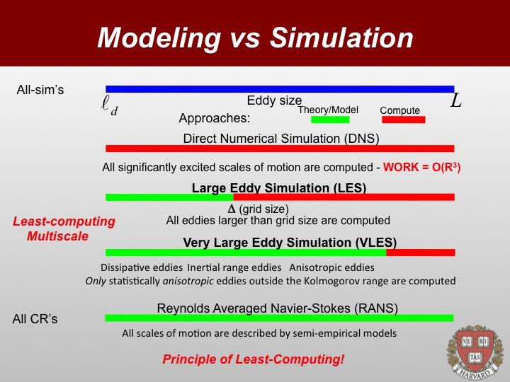
1 Lecture 4: The Navier-Stokes Equations: Turbulence September 23, Goal In this Lecture, we shall present the main ideas behind the simulation of fluid turbulence. We firts discuss the case of the direct numerical simulation, in which all scales of motion within the grid resolution are simulated and then move on to turbulence modeling, where the effect of unresolved scales on the resolved ones is taken into account by various forms of modeling, 1

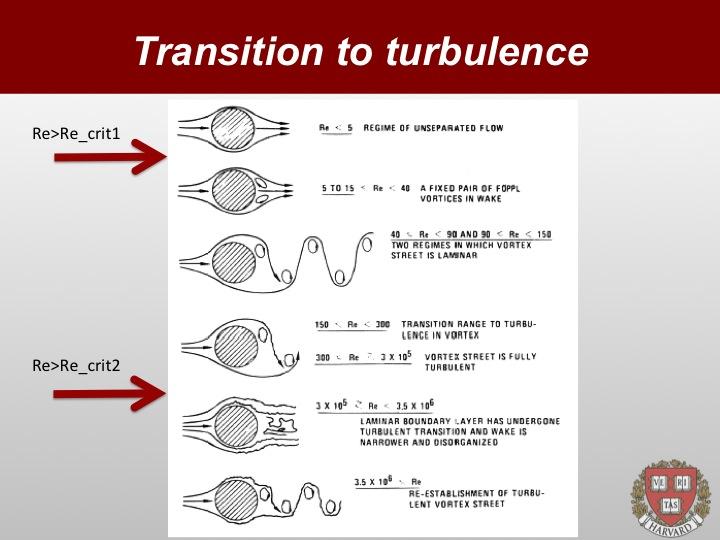
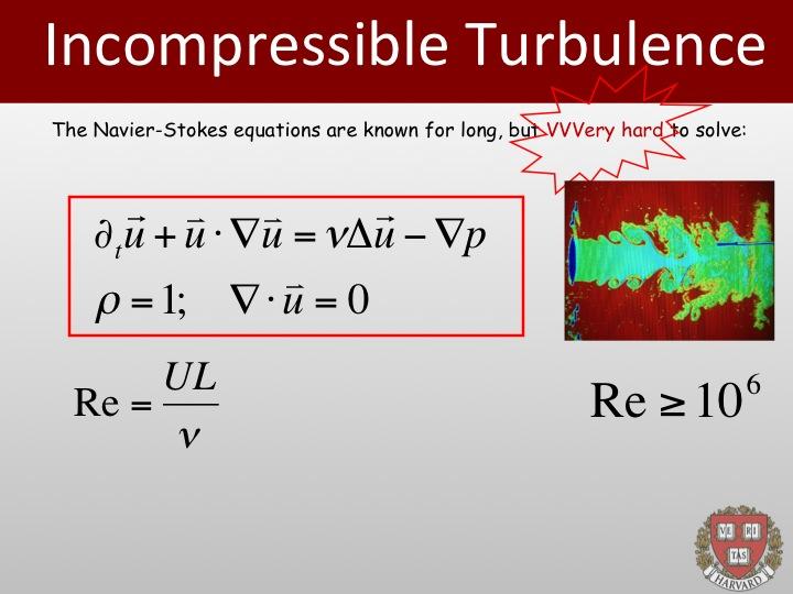
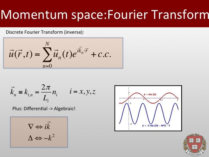
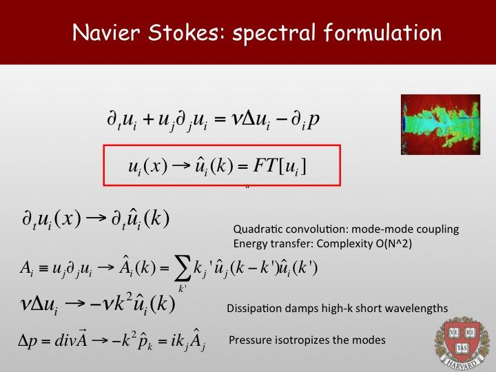
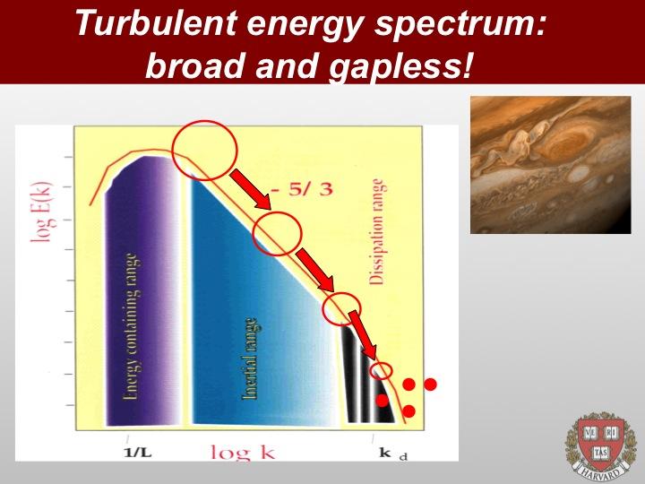
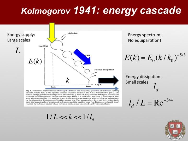
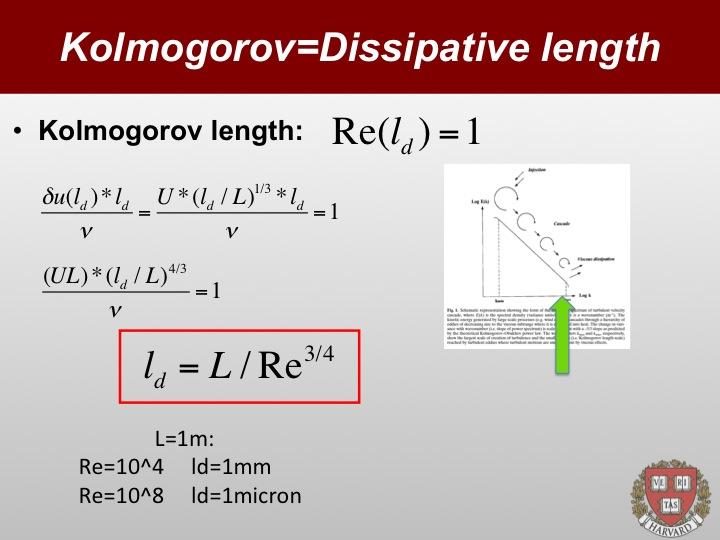
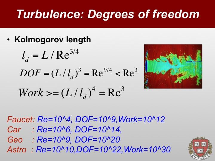
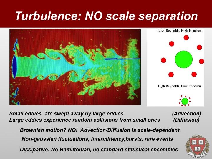
2 2 Fluid turbulence Turbulence is the peculiar state of matter, typical of gases and liquids, characterized by the simultaneous interaction of a broad spectrum of scales of motion, both in space and time. Such simultaneous interaction gives rise to a host of morpho-dynamical complexity which makes the mid/long-term behavior of turbulent flows very hard to predict, weather forecasting possibly offering the most popular example in point. The importance of turbulence, from both theoretical and practical points of view, cannot be overstated. Besides the intellectual challenge associated with the predictability of the dynamics of complex nonlinear systems, the practical relevance of turbulence is even more compelling as one thinks of the pervasive presence of fluids across most natural and industrial endeavours: air and blood flow in our body, gas flows in car engines, geophysical and cosmological flows, to name but a few. Even though the basic equations of motion of fluid turbulence, the Navier-Stokes equations, are known for nearly two centuries, the problem of predicting the behaviour of turbulent flows, even only in a statistical sense, is still open to this day. In the last few decades, numerical simulation has played a leading role in advancing the frontier of knowledge of this over-resilient problem (often called the last unsolved problem of classical physics). To appraise the potential and limitations of the numerical approach to fluid turbulence, it is instructive to revisit some basic facts about the physics of turbulent flows. The degree of turbulence of a given flow is commonly expressed in terms of a single dimensionless parameter, the Reynolds number, defined as Re = UL ν, (1) where U is a typical macroscopic flow speed, L the corresponding spatial scale and ν is the kinematic molecular viscosity of the fluid. The Reynolds number measures the relative strength of advective over dissipative phenomena in a fluid flow: Re u u/(ν u). Given the fact that many fluids feature a viscosity around 10 6 m 2 /s and many flows of practical interest work at speeds around and above U = 1 m/s within devices sized around and above L = 1 m, it is readily checked that Re = 10 6 is commonplace in real life applications. In other words, non-linear inertia far exceeds dissipation, a hallmark of macroscopic phenomena. The basic physics of turbulence is largely dictated by the way energy is transferred across scales of motion. To date, turbulence energetics is best understood in terms of an energy cascade from large scales (l L) where energy is fed into the system, down to small scales where dissipation takes central stage (see Fig.??). This cascade is driven by the nonlinear mode mode coupling in momentum space associated with the advective term of the Navier Stokes equations, u u. 2

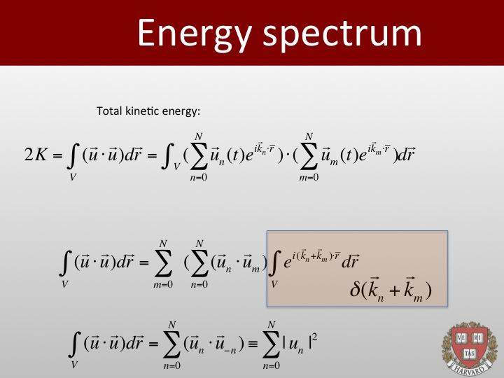
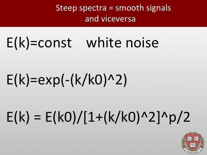
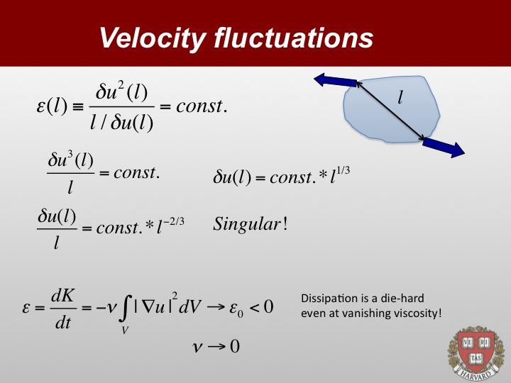
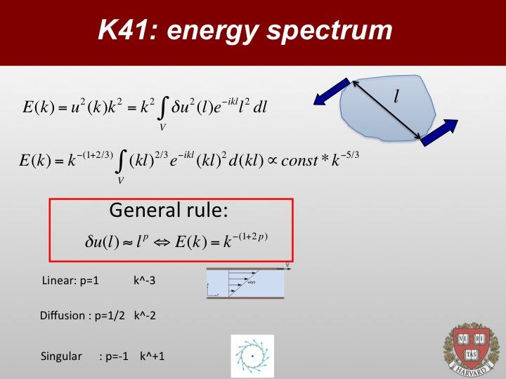
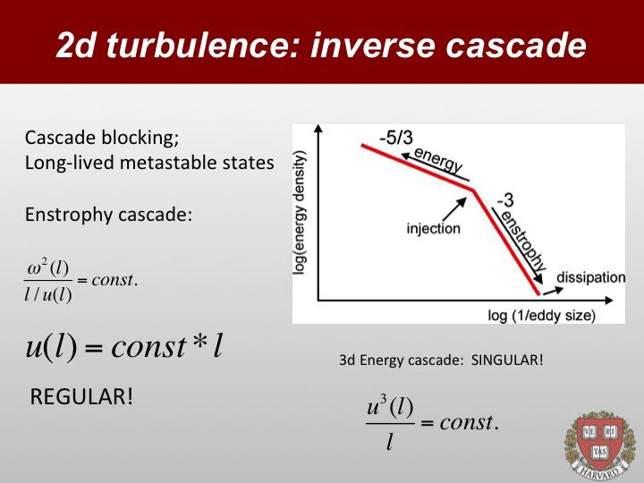
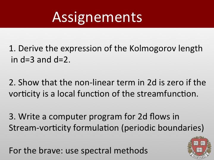
3 In real space, this is the steepening of ocean waves as they approach the shore, we are all familiar with. The smallest scale reached by the energy cascade is known as the Kolmogorov length,, l k, and marks the the point where dissipation takes over advection and organized fluid motion dissolves into incoherent molecular motion (heat). According to the celebrated Kolmogorov (1941) scaling theory [?], the Kolmogorov length can be estimated as: l k L. (2) Re3/4 The estimate (2) follows straight from Kolmogorov s assumption of a constant energy flux across all scales of motion. Let ɛ(l) δu2 (l) τ(l) the rate of change of the kinetic energy associated with a typical eddy of size l (mass=1 for simplicity). By taking τ(l) l/δu(l), we obtain ɛ(l) δu3 (l) l Kolmogorov s assumption of scale invariance then implies: δu(l) = U (l/l) 1/3 where U is the macroscopic velocity at the integral scale L. Note that this realtion implies that the velocity gradient δu(l)/l goes to infinity in the limit l 0, indicating that the flow configuration is singular, i.e. non-differentiable. By definition, the Kolmogorov (or dissipative) length is such that dissipation and inertia come to an exact balance, hence: namely, δu(l k )l k /ν = 1 U (l k /L) 1/3 (l k /L) = ν/l whence the expression (2). The corresponding energy spectrum E(k) u 2 (k), u(k) being the Fourier transform of u(l), is readily computed to scale like E(k) = const. k 5/3, (3) the famous Kolmogorov 5/3 spectrum. The qualitative picture emerging from this analysis is fairly captivating: a turbulent flow in a cubic box of size L, at a given Reynolds number Re, is represented by a collection of N k (L/l k ) 3 Kolmogorov eddies,. By identifying each Kolmogorov eddy with an independent degree of freedom, a quantum of turbulence, (sounds like a good title for the next Bond s 3

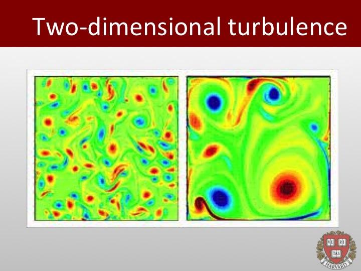
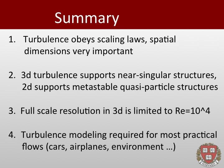
4 movie...), we conclude that the number of degrees of freedom involved in a turbulent flow at Reynolds number Re is given by: N dof Re 9/4. (4) According to this estimate, even a standard flow with Re = 10 6, features more than degrees of freedom, enough saturate the most powerful presentday computers! This sets the current bar of Direct Numerical Simulation (DNS) of turbulent flows, manifestly one falling short of meeting the needs raised by many real life applications. The message comes down quite plain: computers alone won t do! Of course, this does not mean that computer simulation is useless. Quite the contrary, it plays a pivotal role as a complement and sometimes even an alternative to experimental studies. 1 Yet, the message is that sheer increase of raw compute power must be accompanied by a corresponding advance of computational methods. Fluid turbulence is very sensitive to the space dimensionality. For instance, three-dimensional fluids support finite dissipation even in the (singular) limit of zero viscosity, while two-dimensional ones do not. This is rather intuitive, since three dimensional space offers much more morpho-dynamical freedom than two or one-dimensional ones, hence the flow can go correspondingly wilder. Therefore, we shall begin our discussion with two-dimensional turbulence. 2.1 Two-dimensional turbulence As noted above, two-dimensional turbulence differs considerably from threedimensional turbulence. In particular, two-dimensional turbulence supports an infinite number of (Casimir) invariants which can only exist in Flatland. These read as follows: Ω 2p = ω 2p V, p = 1, 2,..., (5) where V ω = u (6) is the vorticity of the fluid occupying a region of volume V. By taking the curl of the Navier Stokes equations, one obtains: D t ω = ν ω + ω u. (7) where D t is the material derivative. It is easily seen that the second term on the right-hand side, acting as a source/sink of vorticity, is identically zero in two dimensions because the vorticity is orthogonal to the flow field. 1 As pointed out by P. Moin and K. Mahesh, DNS need not attain real life Reynolds numbers to be useful in the study of real life applications. (P. Moin and K. Mahesh, Direct numerical simulation: a tool in turbulence research, Ann. Rev. Fluid Mech. 30, 539, 1998.) 4

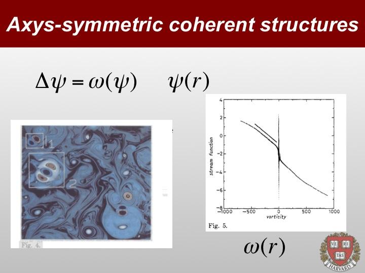
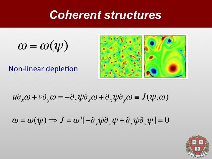
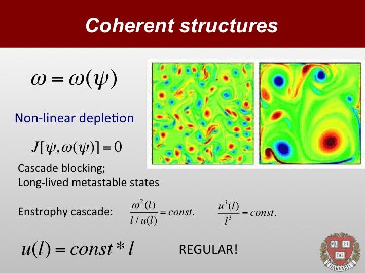
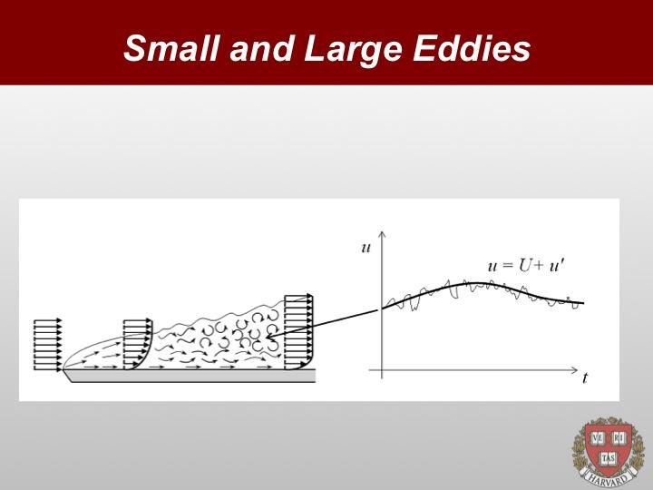
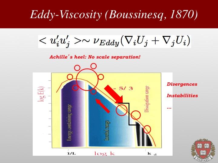
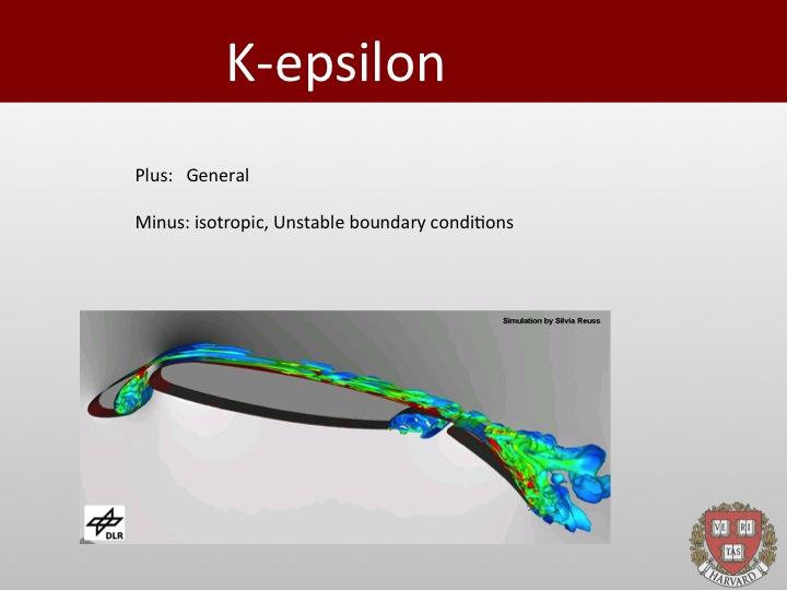
5 As a result, in the inviscid limit ν 0, vorticity is a conserved quantity (topological invariant), and so are all its powers. The fact that vorticity, and particularly enstrophy Ω 2, is conserved has a profound impact on the scaling laws of 2D turbulence. It can be shown that the enstrophy cascade leads to a fast decaying (k 3 ) energy spectrum, as opposed to the much slower k 5/3 fall-off of 3D turbulence. This regularity derives from the existence of long lived metastable states, vortices, that manage to escape dissipation for quite long times. The dynamics of these long-lived vortices has been studied in depth by various groups and reveals a number of fascinating aspects whose description goes however beyond the scope of this Lecture. 3 Turbulence modeling 4 Sub-grid scale modeling Most real-life flows of practical interest exhibit Reynolds numbers far too high to be amenable to direct simulation by present-day computers, and for many years to come. This raises the challenge of predicting the behavior of highly turbulent flows without directly simulating all scales of motion but only those that fit the available computer resolution. The effect of the unresolved scales of motion on the resolved ones must therefore be modeled. To this purpose, it proves expedient to split the actual velocity field into large-scale (resolved) and short-scale (unresolved) components: u a = U a + ũ a (8) and seek turbulent closures yielding the Reynolds stress tensor: σ ab = ρ ũ a ũ b (9) in terms of resolved field U a. Here, brackets denote ensemble-averaging, typically replaced by space-time averaging on the grid. This task makes the object of an intense area of turbulence research, known as turbulence modeling, or sub-grid scale (SGS) modeling. One of the most powerful heuristics behind SGS is the concept of eddy viscosity. This idea, a significant contribution of kinetic theory to fluid turbulence, assumes that the effect of small scales on the large ones can be likened to a diffusive motion caused by random collisions. Small eddies are kinematically transported without distortion by the large ones, while the large ones experience diffusive Brownian-like motion due to erratic collisions with the small eddies. One of the simplest and most popular models in this class is due to Smagorinski [?]. This model is based on the following representation of the Reynolds stress tensor: σ ab = ρν e ( S ) S ab, (10) 5

6 where S ab = ( a U b + b U a )/2 is the large-scale strain tensor of the incompressible fluid and where ν e is the effective eddy-viscosity, defined as the sum of the molecular plus the turbulent one: ν e (S) = ν 0 + ν t (S) (11) The specific expression of the Smagorinski eddy viscosity is as follows: ( ) 1/2 ν e = ν 0 + C S 2 S, S = 2S ab S ab, (12) where C S is an empirical constant of the order 0.1, and is the mesh size of the numerical grid ( = 1 in lattice units). The stabilizing role of the effective viscosity is fairly transparent: whenever large strains develop, σ ab becomes large and turbulent fluctuations are damped down much more effectively than by mere molecular viscosity, a negligible effect at this point. 4.1 Two-equation models The main virtue of the Smagorinski SGS model is simplicity: it is an algebraic model which does not imply any change in the mathematical structure of the Navier Stokes equations. However, it is known to cause excessive damping near the walls, where S is highest. The next level of sophistication is to link the eddy viscosity to the actual turbulent kinetic energy: and dissipation a,b k = 1 2 ũ2 (13) ɛ = ν ( a ũ b ) 2. (14) 2 a,b These quantities are postulated to obey advection diffusion reaction equations of the form [?]: ˆD t k ν k k = S k, (15) ˆD t ɛ ν ɛ ɛ = S ɛ, (16) where ν k, ν ɛ are effective non-linear viscosities for k and ɛ, respectively, and S k, S ɛ are local sources of k and ɛ representing the difference between production and dissipation [?]. Finally, ˆD t t +û a a with û a u a a ν, where ν ν k or ν ν ɛ [?]. These equations constitute the well-known k ɛ model of turbulence, still one of the most popular options for industrial applications. However, the practical use of the k ɛ equations may raise concerns of convergence, due to the non-linear dependence of the eddy viscosities and stiffness of the source terms as well. 6

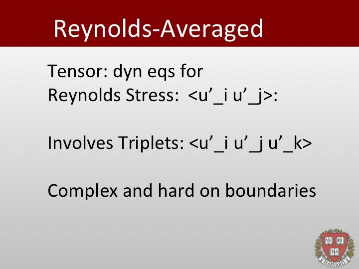
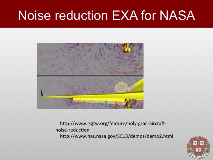
7 4.2 Reynolds-Averaged Navier-Stokes (RANS) The k ɛ model often provides an improvement over Smagorinski, but it is still liable to criticism. In particular, it does not account for the higher directional nature of turbulence near solid boundaries. To cope with this problem, a further level of sophistication is introduced, by formulating dynamic equations for the Reynolds stress itself σ ab. These equations tends to be rather cumbersome, especially in connection with the formulation of proper boundary conditions. Even though they enjoy significant popularity in the CFD engineering community, we shall not delve any further into this option. 5 Summary The modeling of fluid turbulence still stands as one of the major open topics in modern science and engineering. Current computer capabilities allow the full simulation of flows up to Reynolds numbers of the order of 10 4, which is short by several orders of magnitude for many engineering applications, let alone environmental and geophysical ones. To fill thsi gap, teh current practice is extensive resort to various forms of turbulence modeling. 7

8 8

9 9

10 10

11 11

12 12

13 13

14 14

15 15

16 16

17 17

18 18

19 19

20 20

21 21

22 22

23 23

24 24

25 25

26 26

27 27

28 28

29 29

30 30