37 th Benelux Meeting on Systems and Control

Transcription

1 37 th Benelux Meeting on Systems and Control March 27 29, 2018 Soesterberg,

2 The 37 th Benelux Meeting on Systems and Control is sponsored by Raffaella Carloni, Bayu Jayawardhana, and Mircea Lazar (Eds.) - 37 th Benelux Meeting on Systems and Control University of Groningen PO Box AB Groningen All rights reserved. No part of the publication may be reproduced in any form by print, photo print, microfilm or by any other means without prior permission in writing from the publisher. ISBN:

3 Part 1 Programmatic Table of Contents 3

4 4

5 Tuesday, March 27, 2018 Plenary: P0 Welcome and Opening Steyl TuA Closed-loop identification without external excitation W. Yan Eindhoven University of Technology P. Van den Hof Eindhoven University of Technology Chair: Raffaella Carloni Mini Course: P1 Steyl Networks of Dissipative Systems - Part I Murat Arcak Chair: Bayu Jayawardhana Networks of Dissipative Systems - Part I M. Arcak Mini Course: P2 Steyl Networks of Dissipative Systems - Part II Murat Arcak Chair: Bayu Jayawardhanar Networks of Dissipative Systems - Part II M. Arcak TuA01 Steyl System Identification A Chair: Tom Oomen TuA Subspace identification for linear parametervarying systems P. Cox Eindhoven University of Technology R. Toth Eindhoven University of Technology P. Van den Hof Eindhoven University of Technology TuA Identification of LTI models from concatenated data sets S. Vasquez Université Libre de Bruxelles M. Kinnaert Université Libre de Bruxelles R. Pintelon Vrije Universiteit Brussel TuA Local rational method with prior system knowledge: with application to mechanical and thermal systems E. Evers Eindhoven University of Technology B. de Jager Eindhoven University of Technology T. Oomen Eindhoven University of Technology TuA Order estimation of multidimensional transfer function by calculating Hankel intersections B. Vergauwen Katholieke Universiteit Leuven O.M. Agudelo Katholieke Universiteit Leuven B. De Moor Katholieke Universiteit Leuven TuA Prior knowledge and the least costly identification experiment G. Birpoutsoukis Université Catholique de Louvain X. Bombois Ecole Centrale de Lyon TuA02 Angola Optimal Control A Chair: Dimitri Jeltsema TuA A suboptimality approach to distributed linear quadratic optimal control J. Jiao University of Groningen H. Trentelman University of Groningen M. Camlibel University of Groningen TuA Vehicle energy management with ecodriving: A sequential quadratic programming approach with dual decomposition Z. Khalik Eindhoven University of Technology G. Padilla Eindhoven University of Technology T. Romijn Eindhoven University of Technology M. Donkers TuA Power quality: A new challenge in systems and control D. Jeltsema HAN University of Applied Science TuA Spline-based trajectory generation for CNCmachines T. Mercy Katholieke Universiteit Leuven G. Pipeleers Katholieke Universiteit Leuven TuA Optimized thermal-aware workload scheduling and control of data centers T. Van Damme University of Groningen C. De Persis University of Groningen P. Tesi University of Groningen TuA On convexity of the eco-driving problem G. Padilla Eindhoven University of Technology S. Weiland Eindhoven University of Technology M. Donkers Eindhoven University of Technology TuA03 Argentinië Aerospace and Automotive Applications A Chair: Bram de Jager TuA Attitude control of a UAV in presence of motor asymmetry B. Njinwoua Mons University A. Vande Wouwer Mons University 5

6 TuA Longitudinal stability augmentation system for a highly unstable forward swept wing UAV by employing a neutral canard angle M. Creyf Katholieke Universiteit Leuven F. Debrouwere Katholieke Universiteit Leuven M. Versteyhe Katholieke Universiteit Leuven S. Debruyne TuA Control of tethered quadrotors through geodesics 33 T. Nguyen Université Libre de Bruxelles E. Garone Université Libre de Bruxelles TuA Constrained attitude control of rigid bodies via explicit reference governor S. Nakano Université Libre de Bruxelles T. Nguyen Université Libre de Bruxelles E. Garone Université Libre de Bruxelles TuA Design, modeling, and geometric control on SE(3) of a fully-actuated hexarotor for aerial interaction 35 R. Rashad University of Twente P. Kuipers University of Twente J. Engelen University of Twente S. Stramigioli TuA Heat release analysis of advanced combustion concepts M. Oom Eindhoven University of Technology B. de Jager Eindhoven University of Technology F. Willems Eindhoven University of Technology TuA04 Bolivia Distributed Control and Estimation A Chair: Tamas Keviczky TuA Divertor detachment control in nuclear fusion devices T. Ravensbergen Eindhoven University of Technology M. van Berkel Eindhoven University of Technology TuA Unified passivity-based distributed control of mechanical systems L. Valk Delft University of Technology T. Keviczky Delft University of Technology TuA Consensus on the unit sphere, the Stiefel manifold and SO(d): The hunt for almost global convergence 39 J. Thunberg University of Luxembourg J. Markdahl University of Luxembourg J. Goncalves University of Luxembourg TuA A robust consensus algorithm for DC microgrids 40 M. Cucuzzella University of Groningen S. Trip University of Groningen C. De Persis University of Groningen X.Cheng, A. Ferrara, A. van der Schaft TuA Fractional order PI autotuning method applied to multi-agent system R. Cajo Ghent University R. De Keyser Ghent University D. Plaza Escuela Superior Politecnica del Litoral C. Ionescu TuA The normal form: A systematic approach to transform non-convex sets into convex sets A. Cotorruelo Jiménez Université Libre de Bruxelles D. Limón Marruedo Universidad de Sevilla E. Garone Université Libre de Bruxelles TuA05 Botswana Model Reduction Chair: Siep Weiland TuA Model order reduction for drilling automation.. 43 H. Bansal Eindhoven University of Technology L. Iapichino Eindhoven University of Technology W. Schilders Eindhoven University of Technology N. van de Wouw TuA Model reduction of coherent clusters in dynamic power system models J. Leung Université Libre de Bruxelles M. Kinnaert Université Libre de Bruxelles J. Maun Université Libre de Bruxelles F. Villella TuA Model order reduction for an electrochemistrybased Li-ion battery model L. Xia Eindhoven University of Technology E. Najafi Eindhoven University of Technology H. Bergveld Eindhoven University of Technology M. Donkers TuA Synchronization persevering model reduction of Lure networks X. Cheng University of Groningen J. Scherpen University of Groningen TuA Reduced order controller design for disturbance decoupling problems R. Merks Eindhoven University of Technology S. Weiland Eindhoven University of Technology R. Merks Eindhoven University of Technology TuA Error analysis for parametric model order reduction using Krylov subspace method D. Lou Eindhoven University of Technology S. Weiland Eindhoven University of Technology TuA06 Congo Nonlinear Control A Chair: Bayu Jayawardhana

7 TuA Robust stability of feedback linearizable nonlinear systems S. Azizi Université Libre de Bruxelles E. Garone Université Libre de Bruxelles TuA Power-controlled Hamiltonian systems P. Monshizadeh University of Groningen J. Machado SUPELEC R. Ortega SUPELEC A. van der Schaft TuA A port-hamiltonian approach to secondary control of microgrids M. Adibi Delft University of Technology J. van der Woude Delft University of Technology TuA Frequency-driven market mechanisms for optimal power dispatch T. Stegink University of Groningen A. Cherukuri ETH Zurich C. De Persis University of Groningen A. van der Schaft, J. Cortés TuA Hybrid integrator-gain based elements for nonlinear motion control S. van den Eijnden Eindhoven Univ. of Technology M. Heertjes Eindhoven Univ. of Technology H. Nijmeijer Eindhoven Univ. of Technology Y. Knops TuA Formal controller synthesis using genetic programming C. Verdier Delft University of Technology M. Mazo Delft University of Technology TuA07 Mozambique Distributed Parameter Systems Chair: Steffen Waldherr TuA On LQG control of infinite-dimensional stochastic port-hamiltonian systems F. Lamoline University of Namur J. Winkin University of Namur TuA Nonlinear stabilization of infinite-dimensional port-hamiltonian systems applied to repetitive control F. Califano University of Bologna A. Macchelli University of Bologna TuA Port-Hamiltonian formulation of vibrations in a nanorod H. Zwart University of Twente H. Heidari Damghan University TuA Modeling and control of thermo-fluidic processes in spatially interconnected structure A. Das Eindhoven University of Technology S. Weiland Eindhoven University of Technology TuA Dynamic density estimation from cell population snapshot data A. Küper Katholieke Universiteit Leuven R. Dürr Katholieke Universiteit Leuven S. Waldherr Katholieke Universiteit Leuven TuA Stability and passivity of multi-physic systems with irreversible entropy production V. Benjamin Université Catholique de Louvain D. Denis Université Catholique de Louvain N. Hudon Queen s University L. Lefevre TuA08 Kenia System Theory Chair: Eric Steur TuA On representations of linear dynamic networks. 61 E. Kivits Eindhoven University of Technology P. Van den Hof Eindhoven University of Technology TuA Partitioning and stability for linear time-varying large-scale systems T. Pippia Delft University of Technology J. Sijs Delft University of Technology B. De Schutter Delft University of Technology TuA Strong structural controllability of systems on colored graphs J. Jia University of Groningen H. Trentelman University of Groningen M. Camlibel University of Groningen W. Baar TuA Numerical analysis of oscillations in nonlinear networks K. Rogov Eindhoven University of Technology A. Pogromsky Eindhoven University of Technology E. Steur Eindhoven University of Technology H. Nijmeijer TuA Approximate controllability of an axially vibrating nanorod embedded in an elastic medium H. Heidari Damghan University TuA Multiple input multiple output Cepstrum coefficients O. Lauwers Katholieke Universiteit Leuven B. De Moor Katholieke Universiteit Leuven 7

8 Wednesday, March 28, 2018 Mini Course: P3 Steyl Networks of Dissipative Systems - Part III Murat Arcak Chair: Mircea Lazar Networks of Dissipative Systems - Part III M. Arcak Plenary: P4 Steyl Distributed stochastic MPC Tamas Keviczky Chair: Mircea Lazar 10: Distributed stochastic MPC T. Keviczky WeM01 Steyl System Identification B Chair: Johan Schoukens WeM A nonlinear state-space model of the transverse fluid force on an oscillating cylinder in a fluid flow 67 J. Decuyper Vrije Universiteit Brussel T. De Troyer Vrije Universiteit Brussel M. Runacres Vrije Universiteit Brussel J. Schoukens WeM From nonlinear identification to linear parameter varying models: Benchmark examples M. Schoukens Eindhoven University of Technology R. Toth Eindhoven University of Technology WeM Grammar-based encoding of well-posed model structures for data-driven modeling D. Khandelwal Eindhoven University of Technology R. Toth Eindhoven University of Technology P. Van den Hof Eindhoven University of Technology WeM Nonparametric regularization for time-varying operational modal analysis P. Csurcsia Vrije Universiteit Brussel J. Schoukens Vrije Universiteit Brussel B. Peeter Siemens Industry Software NV. WeM A recursive least squares approach to distributed MISO system identification T. Steentjes Eindhoven University of Technology M. Lazar Eindhoven University of Technology P. Van den Hof Eindhoven University of Technology WeM Identification of heat flux components in fusion plasmas M. van Berkel DIFFER T. Kobayashi National Institute for Fusion Science WeM02 Angola Optimal Control B Chair: Mircea Lazar WeM A penalty method algorithm for obstacle avoidance using nonlinear model predictive control B. Hermans Katholieke Universiteit Leuven G. Pipeleers Katholieke Universiteit Leuven P. Patrinos Katholieke Universiteit Leuven WeM Real-time proximal gradient method for linear MPC 74 R. Van Parys Katholieke Universiteit Leuven G. Pipeleers Katholieke Universiteit Leuven WeM Combining optimal sensor and actuator selection with H-inf control design T. Singh Katholieke Universiteit Leuven M. De Mauri Katholieke Universiteit Leuven J. Swevers Katholieke Universiteit Leuven G. Pipeleers WeM Optimal sensor configurations for collision avoidance: A minimax optimization approach R. Mohan Eindhoven University of Technology R. Gielen Philips Healthcare B. de Jager Eindhoven University of Technology WeM Risk-averse risk-constrained optimal control D. Herceg IMT Lucca P. Sopasakis Katholieke Universiteit Leuven A. Bemporad IMT Lucca P. Patrinos WeM Optimal control for a class of differential inclusions 78 J. Eising University of Groningen M. Camlibel University of Groningen WeM03 Argentinië Aerospace and Automotive Applications B Chair: Jan Swevers WeM Driver intervention detection based on vehicle reference dynamics W. Schinkel Eindhoven University of Technology T. van der Sande Eindhoven University of Technology J. Loof Eindhoven University of Technology H. Nijmeijer WeM Motion planning for automated connected vehicles 80 R. van Hoek Eindhoven University of Technology J. Ploeg TNO H. Nijmeijer Eindhoven University of Technology 8

9 WeM String stability analysis of MPC-based heterogeneous platooning J. Reinders Eindhoven University of Technology E. van Nunen TNO E. Semsar-Kazerooni TNO N. van de Wouw WeM Co-design of active controlled systems: Application to state-of-the-art CVT systems C. Fahdzyana Eindhoven University of Technology T. Hofman Eindhoven University of Technology WeM Powertrain design sensitivity study of a heavy-duty hybrid electric truck F. Verbruggen Eindhoven University of Technology T. Hofman Eindhoven University of Technology WeM Feed-forward ALINEA: A ramp metering control algorithm for nearby and distant bottlenecks J. Frejo Delft University of Technology B. De Schutter Delft University of Technology WeM04 Bolivia Distributed Control and Estimation B Chair: Riccardo Ferrari WeM A robust PID autotuning method for steam/water loop in large scale ships S. Zhao Ghent University R. De Keyser Ghent University S. Liu Harbin Engineering University C. Ionescu WeM Controlling triangular formations using angle information L. Chen University of Groningen M. Cao University of Groningen C. Li Harbin Institute of Technology WeM Safe formation-motion control of mobile robots. 87 N. Chan University of Groningen B. Jayawardhana University of Groningen J. Scherpen University of Groningen WeM Distributed constraint optimization for mobile sensor coordination J. Fransman Delft University of Technology B. De Schutter Delft University of Technology J. Sijs Delft University of Technology WeM Coping with collisions in decentralized eventtriggered control M. Balaghiinaloo Eindhoven University of Technology D. Antunes Eindhoven University of Technology WeM Distributed fault and malicious behaviour detection in multi vehicle systems N. Jahanshahi Delft University of Technology R. Ferrari Delft University of Technology WeM05 Botswana Mechanical Engineering A Chair: Bayu Jayawardhana WeM Extending Cummins equation to floater arrays: A port-hamiltonian approach M. Almuzakki University of Groningen J. Barradas-Berglind University of Groningen Y. Wei University of Groningen M. Arias, A. Vakis, B. Jayawardhana WeM Constrained multivariable extremum-seeking applied to optimization of Diesel engine fuel-efficiency 92 R. van der Weijst Eindhoven University of Technology T. van Keulen Eindhoven University of Technology F. Willems Eindhoven University of Technology WeM Reset control for transient performance improvement of systems with friction R. Beerens Eindhoven University of Technology N. van de Wouw Eindhoven University of Technology M. Heemels Eindhoven University of Technology H. Nijmeijer WeM Symbolic equation extraction from SimScape J. Gillis MECO Research Team E. Kikken Flanders Make WeM Nonlinear modeling for analysis of directional drilling processes F. Shakib Eindhoven University of Technology E. Detournay University of Minnesota N. van de Wouw Eindhoven University of Technology WeM Clamping strategies for belt-type CVT systems: An overview S. Prakash Eindhoven University of Technology T. Hofman Eindhoven University of Technology B. de Jager Eindhoven University of Technology WeM06 Congo Nonlinear Control B Chair: Jacquelien Scherpen WeM Capabilities of nonlinear iterative learning control with RoFaLT A. Steinhauser Katholieke Universiteit Leuven J. Swevers Katholieke Universiteit Leuven 9

10 WeM Learning control in practice: Novel paradigms for industrial applications J. Willems Flanders Make E. Hostens Flanders Make B. Depraetere Flanders Make A. Steinhauser, J. Swevers WeM Passivity-based control of gradient systems L. Borja-Rosales University of Groningen J. Scherpen University of Groningen A. van der Schaft University of Groningen WeM Virtual differential passivity based control of mechanical systems in the port-hamiltonian framework R. Baez University of Groningen A. van der Schaft University of Groningen B. Jayawardhana University of Groningen WeM Projective contraction of switching systems G. Berger Université Catholique de Louvain F. Forni University of Cambridge R. Jungers Université Catholique de Louvain R. Sepulchre WeM Nonlinear trajectory tracking via incremental passivity C. Wu Zhejiang University A. van der Schaft University of Groningen J. Chen Zhejiang University WeM07 Mozambique Model-based Control A Chair: Leyla Ozkan WeM Modeling and localized feedforward control of thermal deformations induced by a moving heat load 103 D. van den Hurk Eindhoven University of Technology S. Weiland Eindhoven University of Technology K. van Berkel ASML Netherlands B.V. WeM Ten years of control for nuclear fusion in the Netherlands M. de Baar DIFFER WeM Model-based control of reactive systems using extent-based LPV models C. Mendez-Blanco Eindhoven University of Technology A. Marquez-Ruiz Eindhoven University of Technology L. Ozkan Eindhoven University of Technology WeM Tube-based linear parameter-varying MPC for a thermal system J. Hanema Eindhoven University of Technology R. Toth Eindhoven University of Technology M. Lazar Eindhoven University of Technology WeM Design of distributed thermal actuators for a onedimensional thermomechanical model D. Veldman Eindhoven University of Technology R. Fey Eindhoven University of Technology H. Zwart University of Twente M. van de Wal, J. van den Boom, H. Nijmeijer WeM Design and modeling for controllable UHVCVD. 108 M. Dresscher University of Groningen B. Kooi University of Groningen J. Scherpen University of Groningen B. Jayawardhana WeM08 Kenia Systems Biology Chair: Steffen Waldherr WeM Partial synchronization in networks of Kuramotooscillator networks Y. Qin University of Groningen Y. Kawano University of Groningen M. Cao University of Groningen WeM Integration of protein dynamics in batch bioprocess optimization G. Jeanne SUPELEC S. Tebbani SUPELEC D. Dumur SUPELEC A. Goelzer, V. Fromion WeM Variable selection in linear dynamical systems A. Aalto University of Luxembourg J. Goncalves University of Luxembourg WeM Nonlinear model predictive control of Escherichia coli culture A. Merouane University of Mons S. Tebbani SUPELEC D. Dumur SUPELEC A. Vande Wouwer, L. Dewasme WeM Dynamic constraint-based modelling of bioprocesses: a dynamic flux balance analysis model for recombinant Streptomyces lividans K. De Becker Katholieke Universiteit Leuven K. Bernaerts Katholieke Universiteit Leuven W. Daniels Katholieke Universiteit Leuven K. Simoens WeA01 Steyl System Identification C Chair: Julien Hendrickx

11 WeA Topology identification in dynamic Bayesian networks S. Shi Eindhoven University of Technology G. Bottegal Eindhoven University of Technology P. Van den Hof Eindhoven University of Technology WeA Topology reconstruction of dynamical networks via constrained Lyapunov equations H. van Waarde University of Groningen P. Tesi University of Groningen M. Camlibel University of Groningen WeA Local transfer functions recovery in networked system identification J. Hendrickx Université Catholique de Louvain M. Gevers Université Catholique de Louvain A. Bazanella Univ. Federal do Rio Grande do Sul WeA A sequential least squares algorithm for ARMAX model identification in a closed-loop with sensor noise H. Weerts Eindhoven University of Technology G. Bottegal Eindhoven University of Technology P. Van den Hof Eindhoven University of Technology WeA Sparse identification of linear parameter-varying systems using B-splines D. Turk Katholieke Universiteit Leuven G. Pipeleers Katholieke Universiteit Leuven J. Swevers Katholieke Universiteit Leuven WeA Local module identification in dynamic networks using regularized kernel-based methods K. Ramaswamy Eindhoven University of Technology G. Bottegal Eindhoven University of Technology P. Van den Hof Eindhoven University of Technology WeA02 Angola Optimization Chair: Jan Swevers WeA Computing controlled invariant sets using semidefinite programming B. Legat Université Catholique de Louvain R. Jungers Université Catholique de Louvain P. Tabuada UCLA WeA Decoupling multivariate functions: exploring multiple derivative information J. De Geeter Vrije Universiteit Brussel P. Dreesen Vrije Universiteit Brussel M. Ishteva Vrije Universiteit Brussel WeA Solving multivariate polynomial optimization problems via numerical linear algebra C. Vermeersch Katholieke Universiteit Leuven O. Mauricio-Agudelo Katholieke Universiteit Leuven B. De Moor Katholieke Universiteit Leuven WeA Lookup tables in optimization with CasADi and OptiSpline J. Gillis Katholieke Universiteit Leuven WeA Proximal outer approximation M. De Mauri Katholieke Universiteit Leuven G. Pipeleers Katholieke Universiteit Leuven J. Swevers Katholieke Universiteit Leuven WeA Parametric and robust optimization with OptiSpline 125 J. Gillis Katholieke Universiteit Leuven E. Lambrechts Katholieke Universiteit Leuven G. Pipeleers Katholieke Universiteit Leuven WeA03 Argentinië Robotics A Chair: Mircea Lazar WeA Semantic world modeling for autonomous cars. 126 M. Dolatabadi Eindhoven Univ. of Technology M. van de Molengraft Eindhoven Univ. of Technology M. Steinbuch Eindhoven Univ. of Technology WeA Gearbox design for a flapping twin-wing robot H. Altartouri Université Libre de Bruxelles E. Garone Université Libre de Bruxelles A. Preumont Université Libre de Bruxelles WeA Implementation aspects of time-optimal predictive path following for robot arms N. van Duijkeren Katholieke Universiteit Leuven G. Pipeleers Katholieke Universiteit Leuven M. Diehl University of Freiburg J. Swevers WeA In-eye forbidden-region virtual fixtures based on optical-coherence-tomography-probe proximity measurements Y. Douven Eindhoven Univ. of Technology M. van de Molengraft Eindhoven Univ. of Technology M. Steinbuch Eindhoven Univ. of Technology WeA D path-following using a guiding vector field W. Yao University of Groningen Y. Kapitanyuk University of Groningen M. Cao University of Groningen 11

12 WeA Identification of the time-varying joint impedances for the application to bionic devices G. Cavallo Vrije Universiteit Brussel M. van de Ruit Delft University of Technology A. Schoutens Delft University of Technology J. Lataire WeA04 Bolivia Games and Agent-Based Models A Chair: Tamas Keviczky WeA Resilience against misbehaving nodes in asynchronous networks D. Senejohnny University of Groningen S. Sundaram Purdue University C. De Persis University of Groningen P. Tesi WeA The synchronizing probability function for primitive sets of matrices C. Catalano Gran Sasso Science Institute R. Jungers Université Catholique de Louvain WeA Asynchronous proximal dynamics in multi-agent network games C. Cenedese University of Groningen S. Grammatico Delft University of Technology M. Cao University of Groningen WeA Smart detection and real-time learning in water distribution C. Geelen Wageningen University WeA Evolutionary game dynamics for two interacting populations under environmental feedback L. Gong University of Groningen M. Cao University of Groningen WeA The indefinite soft-constrained differential game revisited J. Engwerda Tilburg University WeA05 Botswana Mechanical Engineering B Chair: Karel J. Keesman WeA Inferential control of a wafer stage using disturbance observers N. Mooren Eindhoven University of Technology N. Dirkx ASML Netherlands B.V. R. Voorhoeve Eindhoven University of Technology T. Oomen WeA Dynamic simulation of ventilated potatoes in large-scale bulk storage facilities N. Grubben Wageningen University K. Keesman Wageningen University WeA Modelling & control of a photopolymerizationbased ceramic additive manufacturing process T. Hafkamp Eindhoven University of Technology B. de Jager Eindhoven University of Technology G. van Baars TNO P. Etman WeA Modeling non-equilbrium multiphase systems A. Romo-Hernandez Université Catholique de Louvain D. Dochain Université Catholique de Louvain N. Hudon Queen s University E. Ydsite WeA Data-driven inverse-model feedforward control using non-causal rational basis functions L. Blanken Eindhoven University of Technology S. Koekebakker OcÃľ Technologies B.V. T. Oomen Eindhoven University of Technology WeA A linear single degree of freedom model for acoustophoresis M. Hakan Kandemir Wageningen Univ. & Research R. Wagterveld Wetsus D. Yntema Wetsus K. Keesman WeA06 Congo Nonlinear Control C Chair: Arjan van der Schaft WeA Lyapunov stability: Why uniform results are important, and how to obtain them E. Lefeber Eindhoven University of Technology WeA Robust automatic generation control in power systems M. Cucuzzella University of Groningen S. Trip University of Groningen J. Scherpen University of Groningen C. De Persis, A. Ferrara WeA On guaranteeing tracking performance and stability with LPV control for nonlinear systems G. Sales Mazzoccante Eindhoven Univ. of Technology R. Toth Eindhoven Univ. of Technology S. Weiland Eindhoven Univ. of Technology 12

13 WeA Performance tuning in extremum seeking control via Lie bracket approximations C. Labar Université Libre de Bruxelles J. Feiling University of Stuttgart C. Ebenbauer University of Stuttgart WeA Nonlinear model order reduction for MPD systems 148 S. Naderilordejani Eindhoven Univ. of Technology B. Besseblink University of Groningen N. van de Wouw Eindhoven Univ. of Technology W. Schilders WeA Construction of PID passivity-based controllers for port-hamiltonian systems L. Borja-Rosales University of Groningen R. Ortega SUPELEC J. Scherpen University of Groningen WeA07 Mozambique Model-based Control B Chair: Simon van Mourik WeA Robust greenhouse climate control W. Kuijpers Eindhoven Univ. of Technology D. Katzin Wageningen Univ. & Research R. van de Molengraft Eindhoven Univ. of Technology S. van Mourik, E. van Henten WeA Flexible bio-hydrogen supply based on model predictive control for balancing an urban hybrid renewable energy system Y. Jiang Wageningen University & Research WeA Model learning predictive control with applications to batch processes M. Loonen Eindhoven Univ. of Technology A. Marquez-Ruiz Eindhoven Univ. of Technology M. Bahadir Saltik Eindhoven Univ. of Technology L. Azkan WeA A model based scenario study for balanced crop irrigation F. Mondaca-Duarte Wageningen University S. van Mourik Wageningen University E. van Henten Wageningen University WeA Supervisory control synthesis for a lock-bridge combination F. Reijnen Eindhoven Univ. of Tech. J. van de Mortel-Fronczak Eindhoven Univ. of Tech. J. Rooda Eindhoven Univ. of Tech. WeA Prediction-based delay compensation for staged crystallization M. Porru Eindhoven University of Technology L. Ozkan Eindhoven University of Technology WeA08 Kenia State Observer and Estimation Chair: Bayu Jayawardhana WeA State estimation for nonlinear systems with communication constraints Q. Voortman Eindhoven University of Technology A. Pogromsky Eindhoven University of Technology H. Nijmeijer Eindhoven University of Technology WeA Cooperative adaptive cruise control: an observerbased approach to increase robustness over unreliable networks F. Acciani University of Twente A. Stoorvogel University of Twente P. Frasca University Grenoble Alpes G. Heijenk WeA Real-time plasma state monitoring and supervisory control on the TCV Tokamak T. Blanken Eindhoven University of Technology F. Felici Eindhoven University of Technology C. Galperti EPFL T. Vu, M. Kong, O. Sauter WeA On experiment design for parameter estimation of equivalent-circuit battery models H. Beelen Eindhoven University of Technology H. Bergveld Eindhoven University of Technology M. Donkers Eindhoven University of Technology WeA A study on recurrent deep learning methods for state of charge estimation in Lithium-Ion batteries 160 E. Najafi Eindhoven University of Technology F. Zanjani Eindhoven University of Technology H. Bergveld Eindhoven University of Technology M. Donkers WeA Similarity-based adaptive complementary filter for IMU fusion A. Andrian Eindhoven Univ. of Technology D. Antunes Eindhoven Univ. of Technology R. van de Molengraft Eindhoven Univ. of Technology M. Heemels 13

14 Thursday, March 29, 2018 Pleanary: P5 Steyl Robot learning Dongheui Lee Chair: Raffaella Carloni Robot learning D. Lee Pleanary: P6 Steyl Robot learning Dongheui Lee Chair: Raffaella Carloni Robot learning D. Lee ThM01 Angola Medical Applications Chair: Julien Hendrickx ThM Modeling and control of pharmacokinetic models 162 P. Themans University of Namur F. Musuamba University of Limoges J. Winkin University of Namur ThM Control and state estimation for MR-guided HIFU hyperthermia D. Deenen Eindhoven University of Technology B. Maljaars Eindhoven University of Technology B. de Jager Eindhoven University of Technology M. Heemels, L. Sebeke, E. Heijman ThM Application of digital technologies in proton therapy treatment: Fast calibration Z. Wang Université Catholique de Louvain Q. Flandroy IBA Group B. Herregods IBA Group R. Jungers ThM EEG classification based on inductive means E. Massart Université Catholique de Louvain S. Chevallier Université de Versailles J. Hendrickx Université Catholique de Louvain P. Absil ThM Quench detection for the cooling system of a particle accelerator for proton therapy B. Dehem Université Catholique de Louvain N. Tran IBA Group F. Glineur Université Catholique de Louvain ThM02 Argentinië Robotics B Chair: Raffaella Carloni ThM Composable skill programming framework for complex sensor-based robot tasks Y. Pane Katholieke Universiteit Leuven W. Decre Katholieke Universiteit Leuven J. De Schutter Katholieke Universiteit Leuven ThM Modelling and control of soft robot manipulators 168 B. Caasenbrood Eindhoven University of Technology H. Nijmeijer Eindhoven University of Technology A. Pogromsky Eindhoven University of Technology ThM Development and implementation of a reconfigurable assembly cell M. Verbandt Katholieke Universiteit Leuven R. Van Parys Katholieke Universiteit Leuven M. Kotzé Katholieke Universiteit Leuven J. Swevers, J. Philips, G. Pipeleers ThM A variable stiffness joint with variable stiffness springs R. Carloni University of Groningen V. Lapp University of Twente A. Cremonese University of Twente J. Belcari, A. Zucchelli ThM A supervisory control and data acquisition (SCADA) system in agriculture and related path planning problems N. Bono Rossello Université Libre de Bruxelles E. Garone Université Libre de Bruxelles A. Gasparri University of Roma Tre R. Carpio ThM03 Bolivia Games and Agent-Based Models B Chair: Bart Besselink ThM Projected-gradient methods for generalized equilibrium seeking in aggregative games are preconditioned forward-backward splitting G. Belgioioso Eindhoven University of Technology S. Grammatico Delft University of Technology ThM Performance comparison of routing strategies for automated guided vehicles V. Mazulina Eindhoven University of Technology A. Pogromsky Eindhoven University of Technology H. Nijmeijer Eindhoven University of Technology ThM Exact potential of nonlinear public good games on networks A. Govaert Eindhoven University of Technology M. Cao Eindhoven University of Technology 14

15 ThM Sets of stochastic matrices with converging products: Bounds and complexity P. Chevalier Université Catholique de Louvain V. Gusev Université Catholique de Louvain J. Hendrickx Université Catholique de Louvain ThM Bursty walkers backtrack M. Gueuning University of Namur R. Lambiotte University of Namur J. Delvenne Université Catholique de Louvain ThM04 Botswana Electro-Mechanical Engineering Chair: Bram de Jager ThM Torsional vibration- and backlash- compensation in drive-lines using non-linear feedforward control 177 C. Vaseur Flanders Make A. Rosich Flanders Make M. Witters Flanders Make B. de Jager ThM Identification of the drive train of an electric vehicle 178 A. De Preter Octinion L. Jacobs MECO Research Team J. Anthonis Octinion G. Pipeleers, J. Swevers ThM Constrained charging of Li-ion batteries A. Goldar Université Libre de Bruxelles R. Romagnoli Université Libre de Bruxelles L. Daniel Couto Université Libre de Bruxelles E. Garone, M. Kinnaert ThM On power grids with grounded capacitors M. Jeeninga University of Groningen ThM Modelling and control of a nanometer-accurate motion system I. Proimadis Eindhoven University of Technology T. Bloemers Eindhoven University of Technology R. Toth Eindhoven University of Technology H. Butler ThM05 Congo Model-based Control C Chair: Leyla Ozkan ThM L2-gain analysis of periodic event-triggered systems with varying delays using lifting techniques 183 N. Strijbosch Eindhoven University of Technology G. Dullerud University of Illinois A. Teel UCSB M. Heemels ThM Systems and control in precision farming: Prospects and challenges S. van Mourik Wageningen University P. Koerkamp Wageningen University E. van Henten Wageningen University ThM LCToolbox - A MATLAB toolbox for robust control design L. Jacobs Katholieke Universiteit Leuven M. Verbandt Katholieke Universiteit Leuven J. Swevers Katholieke Universiteit Leuven G. Pipeleers ThM Effortless NLP modeling with CasADi Opti stack 186 J. Gillis MECO Research Team Event: E1 Steyl DISC Certificates & Best Thesis Award Chair: Henk Nijmeijer Event: E2 Best Junior Presentation Award Steyl Chair: Award Committee Pleanary: P7 Closure Steyl Chair: Organizing Committee Part 1: Programmatic Table of Contents Overview of scientific program Part 2: Contributed Lectures Abstracts Part 3: Plenary Lectures Presentation slides Part 4: List of Participants Alphabetical list Part 5: Organizational Comments Comments, overview program, map ThM Structuring multilevel discrete-event systems modeled with extended finite state automata M. Goorden Eindhoven Univ. of Tech. M. Reniers Eindhoven Univ. of Tech. J. van de Mortel-Fronczak Eindhoven Univ. of Tech. J. Rooda 15

16 16

17 Part 2 Contributed Lectures 17

18 18

19 Subspace Identification for Linear Parameter-Varying Systems P. B. Cox, R. Tóth, and P. M. J. Van den Hof Control Systems Group Eindhoven University of Technology P.O. Box 513, 5600 MB Eindhoven, 1 Introduction In recent years, the linear parameter-varying (LPV) modelling paradigm has been applied to many practical applications to synthesise controllers with performance guarantees even under nonlinear or temporal variations of the underlying system [1]. In the majority of these methods, an LPV state-space (SS) model of the system at hand is required, particularly with static and affine dependence on the scheduling signal. However, identification of such a representation based on observations of the plant is not straightforward and converting other representation based models that might be easier to identify into an SS form suffer from several disadvantages. Popular subspace identification (SID) schemes used for SS model estimation start by identifying a specific input-output (IO) structure using convex optimisation, wherefrom an SS model is constructed by matrix decomposition techniques. Current LPV subspace schemes depend on over-restrictive assumptions and/or the number of the to-be-estimated variables grows exponentially, leading to ill-conditioned IO estimation problems with high computational demand. Therefore, it is currently infeasible to identify moderate to large scale systems with LPV SID schemes. To lower the computational load and ease certain assumptions, we analyse state-of-the-art SID schemes combined with an in-depth examination of LPV IO to SS realisation theory to be able to formulate a unified LPV subspace identification framework and tackle the bottlenecks. 2 Deriving the data-equations Subspace schemes are based on various forms of so-called data-equations, surrogate IO models to represent the underlying system. We will derive such open-loop and closedloop data-equations given that the data-generating system is in the following innovation form (similar to, e.g., [2, 3]): ˇx t+1 = A(p t ) ˇx t + B(p t )u t + K(p t )ξ t, y t = C(p t ) ˇx t + D(p t )u t + ξ t, (1a) (1b) where subscript t is the discrete time, x is the state variable, y is the measured output signal, u denotes the input signal, ξ is a zero-mean white noise process satisfying ξ t N (0,Q) with covariance matrix Q, and A,...,K are affine functions in the scheduling signal, i.e, A(p t )=A 0 + n p i=1 A i p [i] t with p [i] t the i-th element in p t. The to-be-estimated coefficients are {A i,...,k i } n p i=1. The innovation representation (1) can arbitrarily well approximate a representation with independent parameter-varying noise sources on both the state and output equations. The difficulty in applying subspace identification on the derived open-loop and closed-loop data-equations using (1) is that the realization is need to be accomplished under a time-varying observability matrix. 3 Parametric subspace identification To obtain an SS realisation from either the open-loop or closed-loop data-equation, we derive a uniform projection based formulation for the LPV realisation problem established on a maximum-likelihood and stochastic realisation based argument; therefore, extending various well-known linear time-invariant SID schemes to the LPV setting. Furthermore, we show that applying the moving average with exogenous inputs (MAX) IO model set in the LPV openloop identification setting can significantly decrease the complexity of the IO estimation problem for SIDs. In addition, we introduce a basis reduced formulation that can lower the computational complexity significantly in the IO to SS model realisation step. These two new developments lead to better scalable SID schemes. Concluding, we will discuss a unified understanding of LPV subspace identification including LPV IO to SS realisation theory with computationally efficient methods leading to competitive schemes to estimate LPV-SS models. [1] J. Mohammadpour and C. Scherer, editors. Control of Linear Parameter Varying Systems with Applications. Springer, [2] P. Lopes dos Santos, J. A. Ramos, and J. L. Martins de Carvalho. Subspace identification of linear parameter-varying systems with innovation-type noise models driven by general inputs and a measurable white noise time-varying parameter vector. Int. J. of Systems Science, 39(9): , [3] J. W. van Wingerden and M. Verhaegen. Subspace identification of bilinear and LPV systems for open- and closed-loop data. Automatica, 45(2): , This work has received funding from the European Research Council (ERC) under the European Union s Horizon 2020 research and innovation programme (grant agreement No ). 19

20 Identification of LTI models from concatenated data sets Sandra Vásquez 1,2, Michel Kinnaert 1 and Rik Pintelon 2 1 Deparment SAAS (ULB), 2 Department ELEC (VUB) savasque@ulb.ac.be 1 Introduction For some industrial applications, experimental data is available in the form of several data sets corresponding to the operation of the plant under the same conditions. An example of such an application is the condition monitoring of a wind turbine based on SCADA data. Here, one is interested in the identification of a turbine subsystem for a specific wind condition. However, long records of a given operating condition might be difficult to obtain. Hence, one needs to select multiple short data-records from the operational data to identify the system. In this case, identification approaches where missing data are treated as unknown parameters [1, 2] are not feasible due to the large amount of lost data. Then, the best option is to concatenate the data sets, and introduce additional parameters to handle the transient effects [3]. Our aim is to verify the consistency of the estimates when considering this last approach. To this end, we performed a Montecarlo simulation to prove consistency when dealing with AR and ARX model structures. 2 Results The concatenation of M data sets is done as follows x 1 (tt s ) t = 0,...,N 1 1 x 2 (tt s ) t = N 1,...,N 1 + N 2 1 x c (tt s ) =.. x M (tt s ) t = (N N M 1 ),...,N Then, the input/output DFT spectra (U c, Y c ) satisfy Y c ( z 1 ) ( k = G z 1 k,θ ) U c (k) + H ( z 1 k,θ ) ( E (k) + T 1 z 1 k,θ ) +z N ( 1 k T 2 z 1 k,θ ) + + z (N N M 1 ) k T M (Ω k,θ) with G ( z 1 k,θ ) = B ( z 1 k,θ ) /A ( z 1 k,θ ) and H ( z 1 k,θ ) = C ( z 1 k,θ ) /D ( z 1 k,θ ) the plant and noise rational transfer ( function models, and T l z 1 k,θ ) the transient terms. For the( AR and ARX model structures, C = 1, D = A, and T l z 1 k,θ ) ( = I l z 1 k,θ ) /A ( z 1 k,θ ). In addition, B = 0 for the AR case. To verify the consistency on the parameter estimation for both AR and ARX cases, a Montecarlo simulation is performed to compare two situations: the concatenation of data from M experiments (with record length of N m ), and one single experiment (with N = N m M samples). A first order system and transient term are considered (A = 1 + a 1 z 1 k, B = 0 or B = 1, I l = i l ), and the excitation [e(t) or u(t)] is MSE r (db) AR M MSE r (db) ARX M Figure 1: Normalized Mean Square Error MSE r for AR and ARX: concatenated data sets ( ), one data record ( ) white noise with zero mean and unit variance. We tested N m = 2, which corresponds to the extreme case where the data records are just large enough to estimate the parameters. Figure 1 presents the mean square error (MSE) on the estimation of a 1 for different values of M. These results show that for both AR and ARX, the parameter estimation departing from concatenated data is consistent, since the MSE decreases with M at the same rate as the case of one data record. The observed difference on the MSE corresponds to the information loss for the concatenated case. Indeed, for this case one sample out N m is used to estimate the transient coefficient (i l ). Hence, the theoretical difference is db(mse conc /MSE onerec ) = db( N m /(N m 1)). The results for the simulation of both AR and ARX follow well this theoretical difference (3 db, see Fig. 1). Acknowlegment This work is supported by the Fonds de la Recherche Scientifique FNRS (research fellow grant), and is partially supported by the Flemish government (Methusalem grant METH1) and the Belgian federal government (IAP network DYSCO). [1] A. J. Isakkson, Identification of ARX-Models Subject to Missing Data. IEEE Transactions on automatic control, Vol. 38, no. 5, May [2] R. J. A. Little and D. B. Rubin, Statistical Analysis with Missing Data. New York: Wiley, [3] R. Pintelon and J. Schoukens, System identication: A frequency domain approach. IEEE Press,

21 Local Rational Method with prior system knowledge: with application to mechanical and thermal systems Enzo Evers 1, Bram de Jager 1, Tom Oomen 1 1 Eindhoven University of Technology, Department of Mechanical Engineering, Control Systems Technology group PO Box 513, 5600MB Eindhoven,, e.evers@tue.nl 1 Background Frequency Response Function (FRF) identification is fast, inexpensive and accurate, and often used in applications. These FRFs are used either directly, e.g., for controller tuning or stability analysis, or as a basis for parametric identification. Identification of FRFs has been substantially advanced over recent years, particularly by explicitly addressing transients errors. The Local Polynomial Method (LPM) [1] exploits the assumed smoothness of the transient response and approximates locally the transfer function by a polynomial such that the transient can be removed. 2 Problem Consider the output of a LTI system in the frequency domain Y (k) = G(e iω k )U(k) + T (e iω k ) +V (k) (1) where G(e iω k) is the frequency response function of the dynamic system, Y (k),u(k),v (k) are the output, input and noise terms and k denotes the k-th frequency bin. Where T (e iω k) accounts for the transients of both the system response and the noise. An extension of the LPM, the Local Rational Method (LRM) [2, 3] approximates the terms G(e iω k) and T (e iω k) in (1) such that in the local window Y (k + r) = N k+r D k+r U(k + r) + M k+r D k+r +V (k + r) (2) As a consequence of the rational parameterization, the local estimation problem is no longer linear in the parameters which poses additional challenges. The aim of the present paper is to investigate alternative parametrizations, which are also recovered as a special case of the LRM, yet are linear in the parameters while exploiting the advantages of rationally parametrized model structures. 3 Approach Enabling a convex optimization while maintaining the rational parameterization is done by pre-specifying the system poles based on prior knowledge. Consider again a local window around a DFT bin k such that locally G(e iω k+r ) = Nb b=1 θ Gb B b (e iω k+r ), T (e iω k+r ) = Nb b=1 θ Tb B b (e iω k+r ) (3) error [db] LRMP LPM ETFE G Frequency [Hz] Figure 1: Estimation error of the Local Rational Method with Prior knowledge (LRMP) versus the LPM and classical method (ETFE). G 0 denotes the true system. with basis functions B b (e iω k+r) and parameters θ Gb,θ Tb. If the basis functions B b contain the true system dynamics of G(w k+r ) and T (e iω k+r), then the basis in (3) can approximate the system in the local window arbitrarily well. 4 Result A resonant system with two resonance modes is used for simulation. The discrete system has two sets of complex conjugated poles at z 1 = ± i,z 2 = ±0.8581i. An orthonormal basis is composed of single complex poles, e.g., ζ = [ i, i] where ζ are a subset of the poles of the true system. The result in Fig. 1 shows an improved estimation accuracy for both resonance modes. Extensive simulations reveal that the method is robust for inaccurate ζ and for real poles occurring in thermal systems. Acknowledgments Supported by the ATC and NWO-VIDI nr [1] R. Pintelon and J. Schoukens, System identification: a frequency domain approach, 2nd ed [2] D. Verbeke and J. Schoukens, Local parametric modeling based on rational approximation, in 36th Benelux Meeting on Systems and Control, Spa, Belgium, [3] R. Voorhoeve, A. van der Maas, and T. Oomen, Nonparametric identification of multivariable systems: A local rational modeling approach with application to a vibration isolation benchmark, Mechanical Systems and Signal Processing, vol. 105, pp , May

22 Order estimation of multidimensional transfer function by calculating Hankel intersections Bob Vergauwen Oscar Mauricio Agudelo Bart De Moor KU Leuven, Department of Electrical Engineering (ESAT), Stadius Center for Dynamical Systems, Signal Processing and Data Analytics. 1 Introduction Left Right This presentation introduces a data-driven method for determining the order of the transfer function representation of a multidimensional (nd) linear system. A Hankel matrix (referred to as recursive Hankel matrix) is constructed from the available multidimensional data in a recursive way. This work extends the concept of past and future data to nd systems and introduces the concept of mode k left and right data. The intersection between two mode k left and right matrices reveals the order of the system in dimension k. 2 Problem statement In this work the class of nd models is restricted to linear difference equations [1], referred to as PdEs. All equations are defined on a rectangular domain in n dimensions. For a two-dimensional model, the class of linear PdEs is given by, N 1 N 2 i=0 j=0 β i, j y[k 1 + i,k 2 + j] = N 1 N 2 i=0 j=0 α i, j u[k 1 + i,k 2 + j], (1) where k 1 and k 2 are two independent variables. u[, ] and y[, ] are the input and output variables respectively, β i, j and α i, j are the coefficients of the PdE and N 1 and N 2 determine the order of the PdE. Note that the order of the PdE is a tuple: for every dimension the order of the PdE is equal to the highest order of the shift operator. At the basis of the identification algorithm presented in this work lies the concept of the recursive Hankel matrix. This matrix is a block Hankel matrix where all the blocks are Hankel themselves. 3 Intersections between past, future, left and right. The intersection algorithm presented in [2] calculates the intersection between past and future Hankel matrices. For a two-dimensional dataset, past and future is extended with left and right. Graphically the concept of past and future, left and right is shown in Fig. 1. The data matrix is first Hankelized, and afterwards split up in four matrices, past, future, left and right. The intersections between these matrices reveals the order of the PdE. Past Future Fig. 1: Multidimensional transfer functions can graphically be represented by stencils. The dots in this figure represent data points distributed in two dimensions. The solid and dashed lines connecting two points represent linear relations between adjacent data points. By splitting up the data in left-right, past-future some relations are removed, these linear relations are denoted by the dashed lines. 4 Results The main result of this presentation is an algorithm to estimate the order of a PdE on a rectangular grid with a uniform sampling time/distance. The data is Hankelized and split up in different Hankel matrices. Based on the rank of these matrices the order of the PdE is estimated. The presented method for estimating the order of a PdE is demonstrated on a numerical simulation example. Acknowledgements This research receives support from FWO under EOS project G0F6718N (SeLMA) and from KU Leuven Internal Funds: C16/15/059 and C32/16/013. [1] Richard Courant, Kurt Friedrichs, and Hans Lewy. On the partial difference equations of mathematical physics. IBM journal, 11(2): , [2] Marc Moonen, Bart De Moor, Lieven Vandenberghe, and Joos Vandewalle. On-and off-line identification of linear state-space models. International Journal of Control, 49(1): ,

23 Prior Knowledge and the Least Costly Identification Experiment Georgios Birpoutsoukis ICTEAM, Université Catholique de Louvain, B1348 Louvain la Neuve, Belgium Xavier Bombois Laboratoire Ampère UMR CNRS 5005, Ecole Centrale de Lyon, Ecully, France 1 Introduction Optimal input design (OID) is one of the most challenging problems in the field of system identification. In this work, OID for linear systems in the presence of prior knowledge is studied. Information related to exponential decay and smoothness is incorporated in the OID problem by making use of the Bayes rule of information. Three different cases of modeling the linear dynamics are considered, namely Finite Impulse Response (FIR) model with and without prior knowledge, as well as the rational transfer function case. It is shown that the prior information affects the spectrum of the minimum power optimal input. The input with the least power is obtained for the transfer function model case. Figure 1: The optimal input for a linear system in three different cases of model structures. Left: Optimized input spectra for the different model structures. Right: Total power of the optimal input signals. 2 The OID problem A stable linear time-invariant system S 0 is considered in an output error framework such that y = G 0 u + e where y is the measured output, u denotes the input to the system, G 0 is a rational transfer function and e is i.i.d. noise (e N (0,σ 2 e )). The OID problem is defined as: Φ u,opt (ω n ) = arg min Φ u (ω n ) p u(φ u (ω n )) s.t. M total > R adm (ω), ω Φ u (ω n ) 0 ω n (1) where the power spectrum Φ u of the multisine input u is the design variable of the OID problem which is affine in Φ u (ω n ). The first constraint sets a bound on the information matrix M total. It is shown in [1] that accuracy constraints on the identified model can be transformed into a constraint in the form M total > R adm where R adm is in this case a frequency-dependent constraint on the model error achieved at transfer function level of the identified model. In case of prior information available, the total information matrix is given by M total = M + P 1 where M denotes the Fisher matrix representing the information linked to the new experiment and P 1 represents prior information about the identified model. The second constraint is necessary for the signal to be realizable. The optimal design problem (1) is convex in the design variables, therefore there is no risk of resulting in a local minimum. 3 Results The result of the OID problem (1) is depicted in Fig. 1. The optimal input spectrum in case of FIR modeling approaches the one of a white noise signal, as expected. However, when prior knowledge about smoothness of the impulse response is considered, it will suppress the power of the estimated transfer function in the high frequency region. Under this condition, the more relaxed the constraint on the modulus of the transfer function, the more is the prior information able to deliver a model inside the allowable model error bounds. Therefore, the power of the optimal input signal decreases in the high frequency region as the constraint on the transfer function modulus relaxes. 4 Acknowledgments This work was supported in part by the Fund for Scientific Research (FWO-Vlaanderen), by the Flemish Government (Methusalem), the Belgian Government through the Inter university Poles of Attraction (IAP VII) Program, and by the ERC advanced grant SNLSID, under contract [1] Bombois, X., & Scorletti, G. Design of least costly identification experiments: The main philosophy accompanied by illustrative examples. Journal Européen des Systèmes Automatisés (JESA), 46(6-7): ,

24 Closed-loop identification without using external excitation. Wengang Yan, Paul M.J. Van den Hof Control Systems Group,Department of Electrical Engineering, Eindhoven University of Technology, 5600 MB Einhoven, 1 Introduction System identification is a fundamental step in model-based control. Most identification based controller tuning methods use test signals during the identification test. However, test signals disturb process operation, which is a cost in production unit. To reduce the cost of identification, it would be ideal to use no test signal during the identification test. For closed-loop identification, when there is no external excitation, the informative condition must be fulfilled to ensure that the identification criterion has a unique minimum and the parameter estimation is consistent. In this work, the informative conditions are firstly introduced and developed. Then, a method of closed-loop test without using test signals is proposed to achieve the informative condition. Finally, a model error bound is adopted to do the model validation. 2 Informative condition Informativity is a concept that central in identification problems. Loosely speaking, the problem is whether the dataset z(t) allows us to distinguish between different models in model set M(θ). The necessary and sufficient conditions for single-input single-output (SISO) closed-loop systems to produce informative data are discussed by Gevers et al. [1]. In this work, we extend their results to multi-input singleoutput (MISO) closed-loop systems. Note that the multiinput multi-output (MIMO) systems are typically identified as a series of MISO systems. Here, we briefly introduce one main result. Consider the ARMAX model structure, A(q 1 )y(t) = m i=1 B i (q 1 )u i (t) +C(q 1 )e(t) (1) with n a, n b and n c are the degrees of corresponding polynomials, and the controller K(q 1 ) = [ ] S1 (q 1 ) R(q 1 ) Sm(q 1 T ) R(q 1 ), with n s and n r are the degrees of the controller. Then, under some reasonable assumptions, the informative condition for data set z(t) generated by the MISO closed-loop system without external excitation is as follows: max(n s n a,n r n b ) (m 1)n b (2) In summary, for linear time-invariant controller, the informative conditions indicate that the orders of the regulator must be high enough to make the data set generated by the closed-loop system informative. Figure 1: Closed-loop system under shifting controller 3 Method to achieve informativity According to Ljung[2], using nonlinear controllers can make closed-loop systems produce informative data. In this work, the nonlinearity of controller is obtained by using a linear regulator that shifts between different settings, which is shown in Fig. 1. For identification-based control, this method is very useful. Additionally, by developing some proper shifting rules, the control performance of closed-loop system could be improved during identification test. 4 Model validation For a model based control method, model validation is required to check whether the identified model is suitable for control. In [3], a stochastic model error bound is derived based on the asymptotic properties. The model error bound (ω) is given as: G 0 (e jω ) Ĝ(e jω ) (ω) = 3 n h N Φ v (ω)σ 2 e Φ u (ω)σ 2 e Φ ue (ω) 2 (3) To use the error bound, an engineering solution is adopted. This is done by comparing the relative size of the bound with the model over the low and middle frequencies. When the size of bound is smaller than half that of the model, the model can be accepted as a good model. [1] M. Gevers, A. Bazanella and L. Mišković, Identification and the Information Matrix: How to Get Just Sufficiently Rich?, IEEE Transactions on Automatic Control 54(12) (2010), [2] L. Ljung, System identification: Theory for the User, Second Editon, Prentice-Hall, Englewood, Cliffs, NJ, [3] Y. Zhu, Multivariable process identification for MPC: the asymptotic method and its applications, Journal of Process Control 8(2) (1998), 24

25 A Suboptimality Approach to Distributed Linear Quadratic Optimal Control Junjie Jiao, Harry L. Trentelman, and M. Kanat Camlibel Johann Bernoulli Institute for Mathematics and Computer Science, University of Groningen, 1 Introduction In this work, we consider the distributed linear quadratic optimal control problem for multi-agent networks [1], [2]. In this problem, we are given a number of identical agents represented by a finite dimensional linear input-state system, and an undirected graph representing the communication between these agents. Given is also a quadratic cost functional that penalizes the differences between the states of neighbouring agents and the size of the local control inputs. The distributed linear quadratic problem is then to find a distributed diffusive control law that, for given initial states of the agents, minimizes the cost functional, while achieving consensus for the controlled network. This problem is non-convex and difficult to solve, and it is unclear whether in general a solution exists. Therefore, in this work, instead of addressing the version formulated above, we will study a suboptimal version of the distributed optimal control problem. Our aim is to design suboptimal distributed diffusive control laws that guarantee the controlled network to reach consensus and the associated cost to be smaller than an a priori given upper bound. 2 Problem Formulation In this work, we consider a multi-agent system consisting of N identical agents. The underlying graph is assumed to be undirected and connected, and the corresponding Laplacian matrix is denoted by L. The dynamics of the identical agents is given by ẋ i (t) = Ax i (t) + Bu i (t), x i (0) = x i0, i = 1,2,...,N (1) where A R n n, B R n m, and x i R n,u i R m are the state and input of the i-th agent, respectively. We assume that the pair (A, B) is stabilizable. Furthermore, we can rewrite multi-agent system (1) in compact form as ẋ = (I N A)x + (I N B)u, x(0) = x 0 (2) with x = ( x 1,...,x N ), u = ( u 1,...,u N ), where x R nn, u R mn contain the states and inputs of all agents, respectively. Moreover, we consider the cost functional that integrates the weighted quadratic difference of states between every agent and its neighbors, and also penalizes the inputs in a quadratic form, which is given by J(u) = 0 x (L Q)x + u (I N R)u dt, (3) where Q 0 and R > 0 are given real weighting matrices. Our aim is to design a class of suboptimal distributed diffusive control law of the form u = (L K)x, where K R m n is an identical feedback gain for all agents, such that the overall network dynamics ẋ = (I N A + L BK)x (4) reaches consensus and the associated cost J(K) = 0 x ( L Q + L 2 K RK ) x dt. (5) is smaller than an a priori given upper bound. More concretely, we consider the following problem: Problem 1. Consider multi-agent system (2) with associated cost functional (3). Assume the network graph is a connected undirected graph with Laplacian L. Let γ > 0 be an a priori given upper bound for the cost to be achieved. The problem is to find a distributed controller L K so that the controlled network (4) reaches consensus and the cost (5) associated with this controller is smaller than the given upper bound, i.e., J(K) < γ. 3 Main Results We present two design methods for computing suboptimal distributed diffusive control laws, both based on computing a positive semi-definite solution of a single Riccati inequality of dimension equal to the dimension of single agent dynamics. Furthermore, we relax the requirement of exact knowledge of the smallest nonzero and largest eigenvalue of the graph Laplacian by using only lower and upper bounds on these eigenvalues. [1] F. Borrelli and T. Keviczky, Distributed LQR Design for Identical Dynamically Decoupled Systems, IEEE Transactions on Automatic Control, vol. 53, no. 8, pp , Sept [2] D. H. Nguyen, A sub-optimal consensus design for multiagent systems based on hierarchical LQR, Automatica, vol. 55, pp ,

26 Vehicle Energy Management with Ecodriving: A Sequential Quadratic Programming Approach with Dual Decomposition Z. Khalik G.P. Padilla T.C.J. Romijn M.C.F. Donkers departement of Electrical Engineering, Eindhoven University of Technology {z.khalik, g.p.padilla.cazar, t.c.j.romijn, m.c.f.donkers}@tue.nl 1 Introduction Energy consumption of the vehicle is optimized by controlling the power flow between energy storage (e.g. fuel tank and battery), the consumers (e.g. wheels, HVAC, etc) and converters (e.g. internal combustion engine and electric motor). However, in these Vehicle Energy Management (VEM) problems, the vehicle speed is assumed to be given, while most of the power generated by the powertrain is used for propelling the vehicle. Therefore, optimizing the speed of a vehicle over a certain trajectory, thereby allowing for an optimal conversion of potential energy from the road profile into kinetic energy of the vehicle, can lead to a considerable energy consumption reduction. We refer to this latter problem as the ecodriving problem. 2 Energy Management with Ecodriving The ecodriving problem is defined as minimizing traction power P trac over a certain trajectory, subject to the longitudinal vehicle dynamics and some bounds on the speed v and input u, i.e., t f min v(t),s(t),u(t) t 0 { P trac (v(t),u(t))dt, (1a) v(t) = σ u u(t) σ v v(t) 2 σ r gsin(α(s(t))), ṡ(t) = v(t), (1b) v(t) v(t) v(t), u(t) u(t) u(t), (1c) with v(0), s(0), v(t f ), s(t f ) known, and where σ r, σ u, σ v, g are some vehicle dynamics related parameters, s is the distance traveled and α is the road slope. To arrive at a finite dimensional optimization problem, we can discretize (1) using a forward Euler discretization, and arrive discrete-time nonlinear optimal control problem. With the problem in this form, it can solved using Sequential Quadratic Programming (SQP), in which we form a convex SQP subproblem by using linearizing the objective function of the discretetime problem and adding Thikhonov regularization, as well as linearizing the state dynamics. The ecodriving problem can be integrated into the VEM problem, of which an SQP formulation can be made and be decentralized using dual decomposition [1]. This distributed approach is presented in [2] to solve a Complete Vehicle Energy Management (CVEM) problem, in which auxiliary components (e.g. a refrigerated semi-trailer) are added to the energy management Braking Power [kw] Battery Energy [kwh] Vehicle Speed [km/h] Road Altitude [m] Backward Forward Distance [km] Figure 1: Backward vs forward optimization. The dotted lines represent minimum and maximum state constraints. problem [2]. Hence, the SQP and dual decomposition approach presented here lay a foundation to solve the CVEM with ecodriving problem. 3 Results A simulation study for the energy management with ecodriving problem for a series-hybrid electric vehicle is done, and the results are shown in Fig. 1. Here, backward and forward refer to solving the energy management problem with and without ecodriving respectively. We can observe that the amount of braking power is reduced significantly overall, and furthermore, the vehicle speed is now used as a buffer (along side the battery), e.g., the speed is on the lower bound at 4 km, so that the potential energy that is available from 4 km on, is maximally converted to kinetic energy. This allows the fuel consumption to be reduced from l/100 km to l/100 km, which is a decrease of 4,7%, by including the ecodriving into the VEM problem. [1] Khalik, Z., et al. Vehicle Energy Management with Ecodriving: A Sequential Quadratic Programming Approach with Dual Decomposition., Submitted to American Control Conference, [2] Romijn, T. C. J., et al. A distributed optimization approach for complete vehicle energy management., IEEE Transactions on Control Systems Technology,

27 Power Quality: A New Challenge in Systems and Control Dimitri Jeltsema Control Systems Engineering & Reliable Power Supply Faculty of Engineering HAN University of Applied Science Ruitenberglaan 26, 2826 CC, Arnhem, d.jeltsema@han.nl Abstract The increasing use of electrical energy influences the quality of the mains voltage and current, which can cause problems. The quality of the energy supply falls worldwide under the name power quality. A high-quality energy supply can be characterized by the ability to supply a clean and stable grid voltage. A perfect Power Quality ideally ensures low transport losses and a mains voltage that is always available, noise-free and pure sinusoidal, and always within the level and frequency tolerances. Problems with the quality of power have become important for electricity users at all usage levels. The use of non-linear loads and sensitive electronic equipment in both the industrial and commercial sectors and the domestic environment has increased considerably in recent decades. Unfortunately, the same type of equipment often generates disturbances in the energy supply, which in turn affect other devices negatively. In addition to annoying phenomena such as flicker (blinking of light), dips, swells, interruptions, and harmonics in the mains voltage cause machines and other devices to show disruptions, overheat or work inefficiently. Harmonic currents and large asymmetrical loads cause unnecessary capacity and energy losses. The lifespan of machines and other devices is considerably shortened if there is too much fluctuation in the quality of the voltage. In the worst case, entire production lines can fall out, lives in hospitals are at risk, data processing in real time such as the processing of bank transactions can be lost, etc.. According to the Leonardo Power Quality Initiative (LPQI), Power Quality problems in Europe costs a total of 150 billion euros annually and according to research by the Electric Power Research Institute (EPRI) the US sees losses of 119 to 188 billion dollars a year. Contribution In this talk, I will discuss how power quality problems present important opportunities and interesting challenges for the systems and control community. To this effect, I will give a brief overview of the most significant power quality issues today and motivate the need for new tools to tackle them. 27

28 Spline-based trajectory generation for CNC-machines Tim Mercy and Goele Pipeleers MECO Research Team, KU Leuven, Leuven, Belgium DMMS lab, Flanders Make, Leuven, Belgium 1 Introduction In the modern manufacturing industry, Computerized Numerical Control (CNC) machines are commonly used for the production of workpieces. Generally, the workpiece geometry is described as a connection of GCode segments, building its contour. In order to create the workpiece, the machine tool needs to track this contour, requiring a set of trajectories for its axes. Various strategies exist to compute trajectories that let the tool center point trace the contour within the desired accuracy. A popular strategy is to first re-shape the contour, by e.g. rounding sharp corners. Afterwards, the feed rate of the tool along the re-shaped contour is planned, where the rounded shape allows for a higher average velocity [1]. However, this so-called decoupled approach leads to suboptimal results, since the complete problem is not solved in a single step. This abstract presents a novel spline-based trajectory generation method for CNC machines that simultaneously optimizes the workpiece geometry and the tool feed rate. This coupled approach uses an optimal control problem (OCP) formulation to immediately take into account the machine limits like velocity, acceleration and jerk bounds and process limits like the maximum feed rate. In addition, the method directly includes the provided workpiece tolerance by converting it into a tube inside which the machine tool has to stay. Since a lower tolerance inevitably leads to a higher machining time, the method allows making a trade-off between accuracy and productivity, while returning near-optimal trajectories. 2 Methodology The proposed approach computes machine tool trajectories by assigning a separate spline to each GCode segment. This leads to easy contouring constraints that keep the tool inside the tolerance tube. However, when optimizing only one trajectory in each OCP, the tool must come to standstill at the end of each segment, in order to connect any subsequent segment in a smooth way. These decoupled trajectories are suboptimal, except for the case of exact contour tracking (tolerance zero). To avoid decoupling, the proposed method simultaneously optimizes a sequence of N segments by solving a single OCP. Connection constraints impose continuity up to acceleration level at the spline interconnections. In combination with the tolerance tube around each segment, which creates an overlap region between subsequent segments, this allows connecting subsequent segments smoothly (see Figure 1). In addition, the trajectories can exploit the tolerance band, increasing productivity. In order to limit the amount of splines that are optimized simultaneously (N), which reduces the complexity of the OCP, the proposed trajectory generator uses a moving horizon approach. From the computed trajectories for the first N segments, only the one for the first segment is saved. Afterwards, the horizon is shifted, removing segment one from the OCP and adding segment N + 1. The receding horizon approach allows making a good initial guess for all segments. In addition, the presented method exploits spline properties to obtain an efficient problem formulation [2]. Together, this leads to OCP s that require a low solving time. 3 Results Figure 1 shows the computed machine tool trajectories for an anchor-shaped workpiece with a tolerance of 0.5mm. y[mm] x[mm] Figure 1: Anchor-shaped workpiece - machine tool trajectories Acknowledgement This work benefits from KU Leuven-BOF PFV/10/002 Centre of Excellence: Optimization in Engineering (OPTEC), from the project G0C4515N of the Research Foundation-Flanders (FWO-Flanders), from Flanders Make ICON project: Avoidance of collisions and obstacles in narrow lanes, and from the KU Leuven Research project C14/15/067: B-spline based certificates of positivity with applications in engineering. [1] F. Sellmann, Exploitation of tolerances and quasi-redundancy for set point generation. PhD thesis, ETH Zürich, [2] T. Mercy, W. Van Loock, and G. Pipeleers, Real-time motion planning in the presence of moving obstacles, in European Control Conference (ECC), pp ,

29 Optimized thermal-aware workload scheduling and control of data centers Tobias Van Damme, Claudio De Persis, Pietro Tesi ENTEG - Smart Manufacturing Systems University of Groningen Nijenborgh 4, 9747AG Groningen {t.van.damme, c.de.persis, p.tesi}@rug.nl 1 Abstract Recent years have seen a huge increase in online data traffic. Nowadays everything is computed and stored in the cloud. Web giants as Google and Facebook process huge amounts of data on a daily basis. All this processing and storing is done in data centers, halls with thousands of servers. The size of these data centers have increased to the point where they consume megawatts of energy on a yearly basis. With this increase of energy consumption has come a corresponding drive to optimize the control and cooling of a data center such that the operational costs can be kept as low as possible. Major challenges in controlling data centers lie in providing adequate cooling and preventing thermal hot spots from occurring, and optimizing the number of servers which are on at any given time [1, 2, 3]. In an attempt to reduce power consumption, thermal-aware control strategies have been studied and analyzed. The main control objective for a thermal-aware workload scheduler is to keep the temperature of all data processing units below a certain threshold while at the same time maximizing energy efficiency of the system. 2 Thermodynamical Model To address this problem a thermodynamical model of the data center is derived[4]. Following this model, the change of temperature of a part of the data center can then be given by: mc p Ṫ (t) = Q in (t) Q out (t) + P(t) where m is the mass of the air, c p is the heat capacity, Q in (t) is the heat entering the unit, Q out (t) is the heat exiting the unit, and P(t) is the power consumed by the unit. The thermal model directly links the power consumption of the server infrastructure to the temperature changes of the individual components. In the previous work, this model was used to solve an optimization problem that minimizes the energy consumption of the cooling equipment in the data center. Furthermore controllers were designed which steer the data center to this optimal operating point. 3 Project goals 1. A key part in the thermodynamical model are the air flows in the data center. These air flows are chaotic and data-center-dependent, and furthermore difficult to determine. In order to provide a method for finding these parameters, the field of system identification is explored to find proper algorithms to tackle this challenge. 2. The current controllers only work in the interior of the constraint set of the optimization problem. Efforts to extend the controller to operate on the constraint boundaries are done. 3. The theoretical models are integrated into an extensive simulation framework, where the interaction with more heuristic approaches is studied. This is an important stepping stone towards understanding the interaction between different control algorithms and studying the theory behind the combination of these algorithms. [1] N. Vasic, T. Scherer, and W. Schott, Thermal-Aware Workload Scheduling for Energy Efficient Data Centers, Proc. 7th int. conf. on Autonomic computing, 2010, pp [2] Parolini, L. and Krogh, B., A cyber-physical systems approach to data center modeling and control for energy efficiency, Proceedings of the IEEE, 1(2012), 100, pp [3] S. Li, H. Le, N. Pham, J. Heo and T. Abdelzaher, Joint Optimization of Computing and Cooling Energy: Analytic Model and A Machine Room Case Study, 32nd Int. Conf. on Distributed Computing Systems, 2012, pp [4] T. Van Damme, C. De Persis and P. Tesi, Optimized Thermal-Aware Job Scheduling and Control of Data Centers, 20th IFAC World Congress, 2017, Vol. 50, No. 1, pp

30 On Convexity of the Eco-driving Problem G.P. Padilla, S. Weiland, M.C.F. Donkers Control Systems Group, Dep. of Electrical Engineering, Eindhoven University of Technology {g.p.padilla.cazar, s.weiland, m.c.f.donkers 1 Introduction Improving energy efficiency of vehicles is an important topic of research for the automotive industries. The problem of reducing the energy consumption of a vehicle over a certain drive cycle can be formulated as an optimal control problem and its solution is often referred to as an energy management strategy. These strategies are traditionally focused on controlling the power split between the energy buffers and consumers in the vehicle. However, a recent trend is to extend this energy management system to incorporate the vehicle velocity (and thereby the power needed to propel the vehicle) in the optimal control problem; this approach is known as the eco-driving problem. 2 Eco-driving Problem Eco-driving is a driving strategy that aims to increase the energy efficiency of a vehicle. This strategy is the solution to an optimal control problem that aims at obtaining an optimal traction force u(t) and velocity profile v(t) that minimizes the total power P(v,u) consumed by a vehicle while travelling during a given time interval [t o,t f ] over a given trajectory s(t) [s o,s f ] with known geographical characteristics; while being subject to longitudinal vehicle dynamics (1b), non-negative velocity bounds v(t) [ v, v], and boundary conditions on position and velocity. This can be stated in the form of the following optimal control problem: min s(t),v(t),u(t) subject to t f t o P(v(t),u(t))dt (1a) m dv dt = u f (v,s), ds dt = v, s(t o ) = s o, s(t f ) = s f v(t o ) = v o, v(t f ) = v f v v v, (1b) (1c) (1d) (1e) (1f) The consumed power P(v,u) can be obtained from different modeling approaches that capture the energy consumption in the powertrain. In general, (1) is a non-linear optimal control problem that might be nonconvex due to specific features of the vehicle model and road profile. This implies that direct optimization methods or methods based on PMP only provide candidate minima, which might not correspond to the global solution to problem (1). 3 Convexity of the Eco-driving Problem Several methods have been already proposed to solve (1), see, e.g., [1]. However, the literature related to the convexity of the eco-driving problem is scarce. For this reason the work presented in [2] aims to expose a detailed view of the convexity issues of the eco-driving optimal control problem. These results are used to warrant the global optimality of the solution for equivalent convex optimization problems. The main contributions of this research are three fold: First, a method to reformulate and discretize the problem preserving its convexity is presented; second, a set of physically realistic conditions that guarantee a convex (discretized) ecodriving problem are given (see Fig 1; and finally, a sequential quadratic programming method with a convex quadratic programming sub-problem is proposed in order to efficiently solve the eco-driving problem (see Fig. 2). v k [Km/h] Time [s] Figure 1: Certification of convexity (γ φ). 20 Conventional driving Eco-driving s k [Km] Figure 2: Conventional vs. eco-driving profiles. [1] A. Sciarretta, G. D. Nunzio, and L. L. Ojeda, Optimal Ecodriving Control: Energy-Efficient Driving of Road Vehicles as an Optimal Control Problem, IEEE Control Systems, vol. 35, no. 5, pp , Oct [2] G. P. Padilla, Siep Weiland and M. C. F. Donkers, On Convexity of the Eco-driving Problem, Submitted to ACC, h k [m] 30

31 Attitude control of a UAV in presence of motor asymmetry Njinwoua Brice Control Department Mons University Boulevard Dolez 31, Mons Belgium Brice.Njinwoua@umons.ac.be Alain Vande Wouwer Control Department Mons University Boulevard Dolez 31, Mons Belgium Alain.Vandewouwer@umons.ac.be Figure 2: Cascade control. Figure 1: Quadcopter coordinate system. 1 Abstract Quadcopter (Fig. 1), is one of the most used UAVs in both military and commercial in and out-door applications. The stabilisation and the guidance of the quadcopter have been widely study by researchers as they represent a complex problem because of the non linearity of the model and the four control inputs used to control the 6 degrees of freedom of the copter. In this study, a cascade control strategy with PD and PI loop is presented (Fig. 2) to achieve a multirotor stabilization when the electrical actuators have discrepancies in their characteristics. The external disturbance created by the actuator asymmetry is compensated by the PI loop, while the PD loop ensures closed-loop stabilization. The robustness of the control strategy is tested in simulation (Fig. 3) as well as in real-life experiments. [1] Modelling, Simulation and Altitude-Range-Analysis of Quad-copter UAV, Barve et al., 2014 [2] Aerodynamics and control of autonomous quadrotor helicopters in aggressive maneuvering, Huang et al., 2009 [3] Attitude control of a quadrotor, Dikmen et al., 2009 Figure 3: Roll angle : disturbances rejection (10% discrepancy and coupling effects of the Yaw angle). [4] Pitch and Roll control of a Quadcopter using Cascade Iterative Feedback Tuning, Douglas et al., 2016 [5] Different approaches of PID control UAV type quadrotor, Szafranski et al.,2011 [6] The true role of accelerometer feedback in quadrotor control, Martin et al., 2010 [7] Quadcopter physical parameter identification and altitude system analysis, Mustapha et al.,

32 Longitudinal Stability Augmentation System for a highly unstable forward swept wing UAV by employing a neutral canard angle. Mathias Creyf Frederik Debrouwere Mark Versteyhe Stijn Debruyne Department of Mechanical Engineering, M-Group, KU Leuven Campus Bruges, Belgium Introduction Unmanned Aerial Vehicles (UAV) are typically designed to be statically stable, resulting in systems that are easy to fly remotely. Inherent aircraft stability however significantly reduces the maneuverability. In order to cope with this, the authors are designing a Forward Swept Wing (FSW) UAV which shows great maneuverability but is inherently highly unstable around the pitch axis. In order to facilitate the remote piloting of this aircraft, a Stability Augmentation System (SAS) in pitch is hence required. This paper presents the design of the longitudinal SAS, based on the linearized state space model. It will be shown that it is required to incorporate a neutral canard angle in the model in order to meet the targeted response requirements. Setup Description The conceptual design of the forward swept wing UAV is presented in Figure 1. Sweeping the wing forward leads to a span wise lift distribution with more lift closer to the wing root, which reduces the wing bending moment, resulting in a lowered structural weight of the wing. Also, a FSW inherently starts to stall at the wing root. This enhances the low speed handling capabilities of the UAV since the ailerons are not stalled, greatly reducing the risk of entering a spin when the UAV starts to stall. Figure 1: (left) Conceptual design of the FSW UAV. The canard is indicated in orange. (right) Neutral canard angle Since the UAV will be used for high angle of attack flight, the canard offers some advantages. Since it is in front the wing, the canard always experiences clean air and so the UAV does not have the risk of pitch-up tendencies from the blanketing of a conventional tail. Also the canard vortex interacts with the wing, potentially leading to a delay in wing stall and higher lift at and beyond stall. Approach The presented research first focuses on the stabilization of the UAV in the longitudinal direction (pitch); (later adding roll and yaw and the coupling). The goal of the SAS is to stabilize the pitch rate of the FSW UAV while a desired pitch rate can be commanded through the pilot stick. Stabilization is taken care of by a full state feedback controller, which will receive its input from a state observer, since natural responses of an inherent stable UAV are typically specified in open loop pole locations. These open loop pole locations are then considered as the target pole locations of the closed loop stabilized SAS. Tracking of the desired pitch rate will be taken care of by a PI controller. The longitudinal system dynamics are linearized around trim conditions and aerodynamic parameters are estimated from the initial UAV geometry. The state is composed of forward speed, angle of attack, pitch rate and pitch angle, while the input is the canard deflection angle. It was observed that stabilization of the longitudinal dynamics is infeasible with a full state feedback controller for the targeted pole locations obtained for the short period and phugoid modes. Since the UAV is designed to be neutrally stable with the canard removed, the canard should always be more or less parallel to the airflow in order to be able to stabilize the longitudinal dynamics (see Figure 1 (right)). This is referred to as the neutral canard angle. The canard control signal is hence the neutral angle added with the control signal for stabilization and tracking. The authors proposed to embed this neutral canard angle in the system state space equations. The system remains highly unstable but it is now feasible to derive a full state feedback controller which meets the targeted requirements. Results and future work Flight tests were performed with the full non-linear model in Matlab and Simulink. Future work will include identified aerodynamic parameters from wind tunnel tests. Furthermore, since the system is highly nonlinear in the angle of attack a gain scheduling controller will be implemented. Special care will be taken beyond the stall area since then it is possible to exploit the full capabilities of the FSW UAV manoeuvrability. Actuator dynamics will also be considered since now it is assumed that the canard actuator can track the neutral angle and control angle infinitely fast. 32

33 Control of Tethered Quadrotors through Geodesics Tam Nguyen SAAS department Université libre de Bruxelles Av. F. Roosevelt 50, CP 165/55, 1050 Brussels Belgium Emanuele Garone SAAS department Université libre de Bruxelles Av. F. Roosevelt 50, CP 165/55, 1050 Brussels Belgium 1 Abstract This abstract addresses the control problem of quadrotors physically connected to the ground by means of tether cables. The control problem is to stabilize the UAV to a desired position while ensuring that the cable remains taut at all times (see Figure 1). Under the assumption of a massless where m R + 0 is the mass of the UAV, p R3 the position of the UAV, T R + the UAV thrust, R SO(3) the UAV attitude, ẑ := [0,0,1] T the vertical component of the inertial frame, g R + 0 the gravity acceleration, J R+,3 3 0 the moment of inertia of the UAV, ω := [ω x,ω y,ω z ] T R 3 the angular velocity of the UAV, τ R the resultant torque of the UAV, L R + 0 the length of the cable, and q H the quaternion associated to R. We also consider the saturations of the actuators 0 T T max, T max R + 0. (5) The strategy is to use a cascade control approach where the inner loop controls the attitude of the UAV, whereas the outer loop controls its position. More specifically, the outer loop is designed so that the control law: compensates the natural gravity force of the system; ensures that the cable is taut at all times; uses the path of the great-circle navigation called the geodesic path. In order to prove asymptotic stability of the overall control scheme, Small Gain arguments are used. The control scheme is augmented with a nonlinear Reference Governor to enforce constraints satisfaction. Figure 1: Quadrotor tethered to the ground. and inextensible cable and assuming that the cable can be kept taut at all times, the dynamics of the system is the usual model of a UAV [1] subject to a holonomic constraint m p =T Rẑ mgẑ J ω = ω J ω + τ, subject to: p =L, q = 1 2 E(q)ω, (1) (2) (3) (4) [1] Mayhew, Christopher G., Ricardo G. Sanfelice, and Andrew R. Teel. Robust global asymptotic attitude stabilization of a rigid body by quaternion-based hybrid feedback. Decision and Control, 2009 held jointly with the th Chinese Control Conference. CDC/CCC Proceedings of the 48th IEEE Conference on. IEEE, [2] Nicotra, Marco M., Roberto Naldi, and Emanuele Garone. Nonlinear control of a tethered UAV: The taut cable case. Automatica 78 (2017): [3] Nguyen, Tam, and Emanuele Garone. Control of a UAV and a UGV Cooperating to Manipulate an Object. American Control Conference (ACC), IEEE,

34 Constrained Attitude Control of Rigid Bodies via Explicit Reference Governor Satoshi Nakano, Tam Nguyen, Emanuele Garone Service d Automatique et d Analyses des Systèmes Université libre de Bruxelles Avenue Franklin Roosevelt 50, Brussels 1050 Belgium snakano@ulb.ac.be, tanguyen@ulb.ac.be, egarone@ulb.ac.be This paper focuses on the constrained attitude control of a fully actuated rigid body. The dynamics considered is the second order system [1] Ṙ = R ˆω, (1) J ω = (Jω) ω + τ, (2) where R SO(3) is the rotation matrix, ω R 3 the angular velocity, J R 3 3 the inertia matrix and τ R 3 the control torque. Furthermore we define the operator : R 3 so(3) such that x y = x y,x,y R 3 and the inverse operator of as such that (x ) = x, where so(3) is the set of R 3 3 skew-symmetric matrices. We assume that conic constraints are considered [2, 3] Figure 1: Coordinate Frames a T cira bi cosθ ci,a ci,a bi S 2,0 < θ ci < π,i = {1,...n c } (3) where S 2 is the set of the unit sphere on R 3 i.e. S 2 R 3 = {a R 3 a = 1}, a ci the center of the constraint and Ra bi S 2 the direction attached to the body frame Σ b whose configuration is R (see Fig. 1). These constraints represent the restrictions of the pointing directions attached to the rigid body. One of the applications is to avoid damaging sensitive devices e.g. pointing exclusion of cameras towards the sun. The control objective is to design τ in Eq. (2) such that: (i) lim t sk(r T R d ) = 0,sk(A) = 1 2 (A AT ); (ii) for any reference attitude R d (t) SO(3), constraints (3) are satisfied. The proposed control scheme (see Fig. 2) consists of the cascade of two control laws, the first which is tasked with the stabilization of the system (Attitude Control) and the second which takes care of modifying the reference to the attitude control to take into account the constraints. The stabilization control is based on a SO(3) Lyapunov approach based on geodesic arguments. For the constraints satisfaction, we design an Explicit Reference Governor [4] to suitably modify the reference such that constraints are enforced during the transient. All the proposed control laws are defined in terms of rotation matrices in SO(3) and do not make use of any parameterization. Figure 2: Control scheme Acknowledgement This work is supported by WBI, FRIA Ref. 5/FRIA/FC and FNRS MIS Ref. F F-3-5- [1] R. M. Murray, Z. Li, and S. S. Sastry, A Mathematical Introduction to Robotic Manipulation, [2] U. Kalabic, R. Gupta, S. Di Cairano, A. Bloch, and I. Kolmanovsky, Constrained Spacecraft Attitude Control on SO(3) Using Reference Governors and Nonlinear Model Predictive Control, in Proceedings of the 2014 American Control Conference, 2014, pp [3] S. Kulumani and T. Lee, Constrained Geometric Attitude Control on SO(3), International Journal of Control, Automation and Systems, vol. 15, no. 6, pp , [4] E. Garone and M. M. Nicotra, Explicit Reference Governor for Constrained Nonlinear Systems, IEEE Transactions on Automatic Control, vol. 61, no. 5, pp ,

35 Design, Modeling, and Geometric Control on SE(3) of a Fully-Actuated Hexarotor for Aerial Interaction Ramy Rashad, Petra Kuipers, Johan Engelen and Stefano Stramigioli Faculty of Electrical Engineering, Mathematics and Computer Science, University of Twente, Enschede,. r.a.m.rashadhashem@utwente.nl Faculty of Engineering Technology. University of Twente, Enschede,. 3 Geometric Tracking Controller Design Figure 1: The fully actuated hexarotor with the reference frames defined. 1 Introduction Most multi-rotor UAVs currently used, such as quadrotors or hexarotors, are designed and optimized for flying without physical interaction with the environment. This limits the ability to perform complex physical interaction tasks with the environment as it cannot reject arbitrary reaction wrenches from the environment. In this paper, we introduce the design, modeling and control of a fully-actuated omnidirectional hexarotor. The proposed hexarotor has propellers pointing in dissimilar directions optimized by maximizing the generated wrench of the UAV. In addition to the optimization-based design, we also approach the modeling and control design of the proposed UAV in a geometric approach by exploiting the configuration space SE(3) of the UAV. 2 UAV Design In this work, each rotor s orientation is fixed and parametrized by two fixed angles designed to maximize the static generated wrench of the propellers on the UAV s body. Consequently, this maximizes the UAV s agility, payload, and interaction wrench with the environment. Another requirement for an omnidirectional vehicle with fixedlyoriented propellers, is the ability of the rotors to produce thrust bi-directionally. In practice, this can be achieved by variable pitch propellers as in [1] or reversible electronic speed controllers as in [2]. The optimization problem formulation is based on the framework introduced in [3]. The control problem for the class of UAVs under study is to design a control law for the propellers thrusts that enables the tracking of arbitrary trajectories for the UAV s configuration. In order for the controller design methodology to be generic, it will be assumed that the desired control wrench on the vehicle s body results from the control law. Then, in a model-based manner, the desired propellers thrust are computed by the inverse of the mapping between the propellers thrusts and the wrench. This mapping is ensured to be always invertible by the design of the hexarotor. The methodology used in this work for the control system design is based on the framework introduced by Bullo and Murray [4] for geometric tracking on SE(3). A measure of the configuration error between the UAV s configuration and the desired configuration is by an error function, which denotes a positive definite map on the Lie group φ : SE(3) R. The choice for the error function made in this paper yields a coordinate-free controller that is invariant under a change of inertial frame [4]. The designed geometric controller has been simulated on the fully actuated UAV to track a desired position and orientation trajectory from a non-hovering initial configuration. [1] M. Cutler, N. K. Ure, B. Michini, and J. P. How, Comparison of fixed and variable pitch actuators for agile quadrotors, in AIAA Guidance, Navigation, and Control Conference (GNC), vol. 2, [2] D. Brescianini and R. D Andrea, Design, modeling and control of an omni-directional aerial vehicle, in 2016 IEEE Int. Conf. Robot. Autom. IEEE, may 2016, pp [3] S. Park, J. Her, J. Kim, and D. Lee, Design, modeling and control of omni-directional aerial robot, in 2016 IEEE/RSJ Int. Conf. Intell. Robot. Syst. IEEE, oct 2016, pp [4] F. Bullo and R. M. Murray, Tracking for fully actuated mechanical systems: a geometric framework, Automatica, vol. 35, no. 1, pp ,

36 Heat Release Characterization for Advanced Combustion Concepts Michiel Oom, Bram de Jager, Frank Willems Eindhoven University of Technology PO Box 513, 5600 MB Eindhoven, 1 Introduction The worldwide demand for diesel in the transportation sector is projected to continue to grow until 2040 [1]. Furthermore, the energy usage of freight trucks is projected to increase with 50% in 2040 compared to It is therefore important to keep on improving the fuel consumption and emissions of internal combustion engines. Whilst in conventional Diesel engines there exists a tradeoff between fuel economy and emissions, advanced combustion concepts allow for a simultaneous improvement of these two aspects. These concepts rely on the spontaneous auto-ignition of a relative homogeneous air-fuel mixture. The control objective is to condition the mixture such that the ignition is well timed. Figure 1 shows a widely used combustion control scheme. Using the first law of thermodynamics for closed systems, the combustion heat release is inferred from an in-cylinder pressure measurement. Combustion metrics are extracted from the heat release profile and controlled using the fueling strategy. 3 Proposed Characterization In this study, a new characterization for the heat release profile is proposed. This characterization consists of a superposition of three Gaussian curves, complying with the three combustion phases, given by: Q combustion (θ) = 3 i=1 a i e (θ b i) 2 /(c 2 i ), (1) where θ [ 360,360) [ ] is the crankshaft angle and a i, b i, c i R, i = 1,2,3, the proposed combustion metrics. Figure 2 (bottom) shows this characterization (red) for a measured heat release signal (blue) and the remaining signals are the components of the fit. In the accompanying presentation, a wide range of operating conditions are analyzed using the proposed metrics. Furthermore, the role of these metrics in control oriented models is examined. Finally, an outlook is given to the design of the controller. reference metrics + controller metric extraction metrics fueling strategy heat release engine first law analysis in-cylinder pressure Figure 1: Advanced combustion concept control scheme. 2 Current Combustion Metrics Figure 2 (top) shows commonly used combustion metrics. These metrics, θ 10, θ 50 and θ 90, point out the crankshaft angles at which 10%, 50% and 90% of the total heat is released. These comply closely with the start, the weight and the end of combustion. However, they do not fully define the actual shape of the heat release, which varies greatly in advanced combustion concepts. Shaping this heat release is crucial in optimizing the thermal efficiency of the engine. The current understanding, originating from fundamental combustion research, divides the combustion process in a premixed, rate-controlled and late combustion phase. Different emission formation and reduction mechanisms are assigned to these three phases. Figure 2: Current and proposed combustion metrics. [1] U.S Energy Information Administration (2016), International Energy Outlook 2016 with Projections to

37 Divertor detachment control in nuclear fusion devices T. Ravensbergen M. van Berkel Dutch Institute for Fundamental Energy Research, De Zaale 20, 5612 AJ Eindhoven, 1 Particle exhaust in tokamaks One of the open issues on the road to viable and clean energy production via nuclear fusion is the heat and particle load on the inner wall of the device. In a tokamak, magnetic fields are used to confine the hot plasma in which hydrogen atoms are fusing to form helium and great amounts of energy. The bottom part of the reactor, called the divertor, acts as a helium exhaust. Plasma from the hot core drifts radially outwards, entering a thin region called the scrapeoff-layer (SOL). Here, the plasma rapidly flows towards the divertor target plates. Without precaution, the resulting heat load can be up to 150 MWm 3, greatly exceeding the engineering limit of 10 MWm 3 [1]. A promising but challenging solution is to increase the plasma density in the divertor via neutral (impurity) gas puffing. This leads to stagnation of the plasma flow, and high power and momentum losses, causing the temperature to drop significantly along the field line. As such, the plasma extinguishes near the divertor target, leading to so-called divertor detachment. Even though the precise physics of detachment are not yet fully understood, different loss mechanisms such as impurity radiation, ionization, and recombination dominate at different temperatures, causing various fronts to arise. These fronts are indicated by different colors in Figure 1). Figure 1: Schematic view of the divertor plasma, including detachment fronts. 2 Controlling plasma detachment While plasma detachment evidently leads to significantly lower target temperatures and particle fluxes, experiments on machines existing today show that it is difficult to control the location of the detachment front [2]. Depending on the divertor geometry and other machine characteristics, the front is often observed to move inside the confined plasma region, affecting the plasma stability and fusion performance. Hence, the challenge is to measure the front location and control the uncertain dynamics of detached plasmas using slow actuators (gas puffing). In this work, we focus on a carbon machine in operation today called MAST-U. 3 Diagnostic development for MAST-U A promising solution to locate the detachment front is multispectral imaging, where multiple cameras equipped with spectral filters observe the same portion of the divertor plasma [3]. Carbon will be the prominent radiating species in a carbon machine, such that a high intensity region in a CIII-filtered image is likely to be an excellent estimate of the radiation front. At the same time, other spectral lines provide information on recombination and ionization [4]. In this work, we apply standard multiscale edge detection based on wavelets [5] to first detect the plasma edge in realtime. Then, along this edge, another wavelet-based detector is employed to locate the radiation front. Finally, using a coordinate transform [6], we can map this front location to the poloidal plane, yielding our to-be controlled variable. The next step involves a set of dedicated system identification experiments on the MAST-U tokamak in the UK. This data will provide a basis for simple controller design, and possible benchmark of control-oriented models. [1] Wenninger, R.P. et al Nuclear Fusion 54 [2] Potzel, S. et al Journal of Nuclear Materials 438 S285 [3] Vijvers, W.A.J. et al Journal of instrumentation 12 C12058 [4] Verhaegh, K. et al Nuclear Materials and Energy [5] Van Berkel, M. et al Fusion Engineering and Design [6] Hommen, G Optical boundary reconstruction for shape control of tokamak plasmas Ph.D. thesis Eindhoven University of Technology 37

38 Unified Passivity-Based Distributed Control of Mechanical Systems Laurens Valk and Tamás Keviczky Delft Center for Systems and Control, Delft University of Technology Introduction Passivity-based control is a well-established method for controlling fully-actuated mechanical systems such as robotic manipulators. Relying on concepts such as energy storage, routing, and dissipation, many design procedures exist to achieve a control goal with guaranteed stability properties. Using similar passivity arguments, several distributed control strategies have been developed to cooperatively control networks of such systems, in order to achieve control goals such as state synchronization or formation forming [1 4]. While these distributed control methods are derived from similar passivity principles, the control laws differ depending on the desired group behaviors (synchronization or formation), the information exchange (positions and/or velocities), the method of energy dissipation (by the network, the agents, or both), and the presence of a group reference. We present a unified control scheme that encompasses the methods [1 4] for fully-actuated mechanical systems in a connected, undirected network without time delays (Fig. 1). Unified Control Scheme As common in robotics literature, a fully-actuated agent i with coordinates q i R n is assumed to have the dynamics M i (q i ) q i +C i (q i, q i ) q i + G i (q i ) = τ i (1) with a control input τ i R m and an output y i R m given by y i = ẋ i v with ẋ i = q i +Λq i, v = q d (t)+λq d (t) (2) where Λ 0. The reference signals q d and q d are either given as functions of time or set to zero, depending on the group objective. Each agent uses a control law of the form τ i = G i + M i ( v Λ q i ) +C i (v Λq i ) κy i + u i (3) to render the system passive from the new input u i to output y i. It is lossless if κ = 0 or strictly output passive if κ > 0. The difference variable z k = x i x j associated with the bidirectional edge k is a measure of distance between agent i and j. The distributed control goal is to ensure that either all z k converge to specified target sets, or that all y i converge to one another. This is accomplished by using the control law u = (D I m )(ψ(z) + φ(ż)) (4) where D is the incidence matrix of the network. The functions ψ( ) and φ( ) are cf. [1] and [2], and can be conceptualized as virtual spring and damper forces, respectively. 1 N v ẋ + + y D I m κ ż φ(ż) ż z + u ψ(z) + D I m y i τ i + u EL i i G i + M i ( v Λ q i ) +C i (v Λq i ) + u i i = 1,...,N κ Λ q d q d φ ψ Storage Dissip. Exch. [1] > 0 = 0 n/a q d = 0 0 both agents q i [2] = 0 > = 0 agents network q i, q i [3] > 0 > 0 q d q d 0 = 0 agents both q i, q i [4] > 0 = both both q i, q i Fig. 1: Unified control scheme extended from [1], and the specializations to obtain the control laws u i of [1 4]. Energy Storage and Dissipation The unified scheme facilitates a comparison of the methods, as done here for energy storage and dissipation. In [1, 4], coupling between the coordinates q i and q j is achieved by virtual spring forces ψ k (z k ) generated as gradients of the energy stored in the network, whereas in [2, 3] it is accomplished due to Λ > 0, which implies synchronization of all q i if all y i synchronize. Likewise, energy can be dissipated by the agents when choosing κ > 0 as in [1, 3, 4] or by the network when choosing ż k φ k(ż k ) 0 as in [2, 3, 4]. [1] M. Arcak, Passivity as a design tool for group coordination, IEEE Transactions on Automatic Control, vol. 52, no. 8, pp , 2007 [2] M. W. Spong and N. Chopra, Synchronization of networked Lagrangian systems, Lagrangian and Hamiltonian Methods for Nonlinear Control. LNCIS, vol. 366, 2007 [3] S. J. Chung and J. J. E. Slotine, Cooperative robot control and concurrent synchronization of Lagrangian systems, IEEE Tr. Robotics, vol. 25, no. 3, pp , 2009 [4] W. Ren, Distributed leaderless consensus algorithms for networked EulerLagrange systems, International Journal of Control, vol. 82, no. 11, pp , 2009 u 38

39 Consensus on the unit sphere, the Stiefel manifold and SO(d): the hunt for almost global convergence Johan Thunberg, Johan Markdahl, and Jorge Gonçalves Luxembourg Centre for Systems Biomedicine University of Luxembourg 6, avenue du Swing, L-4367 Belvaux, Belvaux Luxembourg {johan.thunberg, johan.markdahl, 1 Introduction For the Euclidean space well-established convergence results are available for consensus systems dating back more than a decade. There is a collection of such results stating that if individual agents in the system are moving into the convex hulls of their neighbors positions, the states will aggregate over time and finally all converge to a fixed point, i.e., the consensus point or the synchronization point. Those results hold under weak connectivity assumptions for possible time-varying interaction network. For multi-agent systems evolving in other spaces than the Euclidean, the equivalent convergence result does not hold in general. Examples of such non-euclidean spaces are the unit sphere, the Stiefel, and the special orthogonal group. Those are all interesting from application perspectives. Consensus on the unit sphere can be seen as equivalent to heading-alignment of multi-robot systems as well as systems in nature. Also the problem of synchronization of phase oscillators is closely related to that of consensus on the unit circle. Consensus of orthogonal matrices is an active research topic, also referred to as attitude synchronization within the application of rigid bodies in space. Consensus on the Stiefel manifold can be seen as a problem residing between the other two, i.e., with the unit sphere and the special orthogonal group as extremes. 2 New convergence results We aim to bring two recent papers to the forefront [1, 2] as well as discuss possible generalizations thereof. They provide new controllers and convergence results to the aforementioned consensus control problems. It used to be a held belief that a globally convergent consensus controller on the unit sphere could not be based on purely relative and local (and intrinsic) information. Previous works have shown that classical geodesic control laws on the unit circle fail to achieve almost global convergence. Various approaches have been suggested to overcome this. Examples of such include so-called shaping functions or the introduction of estimation variables. However, as shown in [1], the unit circle comprises an odd exception to the rule. In fact for all unit spheres of dimensions larger than or equal to 2, classical geodesic control laws using only relative and local information achieves consensus almost globally for undirected graph topologies and symmetric weights. Furthermore, these weights do not need to be constant, but can be chosen as a non-negative nonlinear functions of the relative distance between agents. The result in [1] are perhaps non-intuitive based on what was previously known about the convergence on the circle. In [2] we provide a collection of synchronization controllers for all the three manifolds mentioned in the introduction. The interaction graph of the multi-agent system is assumed to be quasi-strongly connected. We show that the closed loop systems under the controllers achieve almost global convergence to the consensus set. However, the convergence results come at price. Even though only relative information is used in terms of the states, we introduce additional estimation variables that are communicated between neighboring agents. This approach is all but new, however here we do it in a way that makes the same approach applicable for the unit sphere and the special orthogonal group as well as all the Stiefel manifolds in between; we use the QRdecomposition of a matrix. This allows to obtain a closed loop dynamics that is on strict feedback form, where the dynamics of the k first columns are decoupled from the remaining ones. With these results as a starting point, we also aim to investigate further generalizations such as extensions of the results in [1] to the Stiefel manifold. [1] Johan Markdahl, Johan Thunberg, and Jorge Gonçalves. Almost global consensus on the n-sphere. IEEE Transactions on Automatic Control, [2] Johan Thunberg, Johan Markdahl, and Jorge Gonçalves. Dynamic controllers for column synchronization of rotation matrices: a QR-factorization approach. To appear in Elsevier s Automatica. 39

40 A robust consensus algorithm for DC microgrids M. Cucuzzella, S. Trip, C. De Persis, X. Cheng, A. Ferrara, A. van der Schaft University of Groningen, Nijenborgh 4, 9747 AG Groningen, University of Pavia, via Ferrata 5, Pavia, Italy University of Groningen, Nijenborgh 9, 9747 AG Groningen, Abstract DGu i Line i j In the last decades, due to economic, technological and environmental aspects, the main trends in power systems focused on the modification of the traditional power generation and transmission systems towards incorporating smaller Distributed Generation units (DGus). Moreover, the everincreasing energy demand and the concern about the climate change have encouraged the wide diffusion of Renewable Energy Sources (RES). The so-called microgrids have been proposed as conceptual solutions to integrate different types of RES and to electrify remote areas. Two main control objectives in DC microgrids are voltage regulation and current sharing (or, equivalently, load sharing) [1]. This work proposes a novel robust control algorithm to obtain simultaneously proportional current sharing among the DGus and a form of voltage regulation in a resistiveinductive DC power network, independently of the initial voltage conditions, facilitating Plug-and-Play capabilities. In order to achieve current sharing, a communication network is exploited where each DGu communicates in realtime the value of its generated current to its neighbouring DGus. The overall network is represented by a connected and undirected graph G = (V,E), where the nodes, V = {1,...,n}, represent the DGus and the edges, E = {1,...,m}, represent the distribution lines interconnecting the DGus. The network topology is represented by its corresponding incidence matrix B R n m. Consequently, the DC microgrid system can be written compactly for all nodes i V as L t İ t = R t I t V + u C t V = I t + BI I L Lİ = B T V RI, where I t,v,i L,u R n, I R m, while C t,l t,r t R n n and R,L R m m are positive definite diagonal matrices. The meaning of the symbols used in (1) follows straightforwardly from Fig. 1. Now, we make the considered control objectives explicit: Objective 1 (Proportional Current sharing) (1) lim t I t(t) = I t = W 1 1 n i t, (2) V DCi Buck i u i R ti I ti L ti C ti PCC i Figure 1: The considered DC microgrid electrical scheme. where i t = 1 T n I L /(1 T n W 1 1 n ) R, W = diag{w 1,...,w n }, w i > 0, for all i V, and 1 n R n is the vector consisting of all ones. Objective 2 (Voltage balancing) lim t 1T n W 1 V (t) = 1 T n W 1 V = 1 T n W 1 V, (3) where V R n is the voltage reference. In order to achieve Objectives 1 and 2 simultaneously, we constrain the state of system (1) on the following desired manifold: V i {(I t,v,i,θ) : W 1 (V V ) θ = 0}, (4) where θ R n is an additional state variable (distributed integrators), with dynamics given by I Li R i j θ = L c WI t, 1 T n θ(0) = 0 (5) L c denoting the weighted Laplacian matrix associated with the (undirected and connected) communication graph, which can be different from the topology of the microgrid. To constrain the state of the system (1) to the designed manifold (4) in a finite time, we propose robust controllers of Sliding Mode type [2]. [1] C. De Persis, E. R. A. Weitenberg, F. Dörfler, A power consensus algorithm for DC microgrids, Automatica, [2] V. I. Utkin, Sliding Modes in Control and Optimization, Springer-Verlag, I i j L i j 40

41 Fractional Order PI Autotuning Method Applied to Multi-Agent System Ricardo Cajo 1,2, Robin De Keyser 1, Douglas Plaza 2 and Clara M. Ionescu 1 1 Research group on Dynamical Systems and Control, Ghent University, Belgium 2 Facultad de Ingeniería en Electricidad y Computación, Escuela Superior Politécnica del Litoral Campus Gustavo Galindo Km 30.5 Vía Perimetral, P.O. Box , Guayaquil, Ecuador RicardoAlfredo.CajoDiaz@UGent.be 1 Introduction In order to significantly improve operational efficiency, reduce costs and increase the degree of operational redundancy. Hence, multi-agent systems (MAS) are widely used in the construction of complex systems. Therefore, they are being widely recognized as new technologies for the next generation of distributed and intelligent industrial automation systems [1]. The distributed control systems approach is preferable for the development of applications that involve multiple autonomous units, which have to communicate with each other to achieve the common goal through their coordinated actions. 2 Control Strategies A novel fractional order PI autotuner based on KC method [2] is applied to the multi-agent systems. This method consists in defining a forbidden region in the Nyquist plane based on user-defined specs, which will guarantee the system margin requirements. Its performance is compared with two other fractional order controllers based on PI gaincrossover autotuning method [3] and Internal Model Control (IMC) present in [4]. A numerical example considered is described by the following transfer function G(s) mimicking a part of a multi-agent flock: G(s) = s s s s+1 ;Λ = [ Checking input-output pairings, with a RGA (Relative Gain Array) analysis of the multivariable process. Its matrix Λ suggest that the pairing 1-2/2-1 is suitable, since the main diagonal has negative values 3 Results and Conclusions According to results shown in Figure 1 and Figure 2, the KC method produces fractional order PI controllers that achieve excellent load disturbance rejection, while maintaining a good reference tracking performance. It is important to note ] (1) that the proposed method does not use the full knowledge of the system model. However, this shows that the KC method could obtain similar or better results than other controllers, which use the full knowledge of the system. Output 1 Output FO PI FO IMC FO KC Time[min] FO PI FO IMC FO KC Time[min] Figure 1: Comparative setpoint tracking test Output 1 Output FO PI FO IMC FO KC Time[min] FO PI 11.2 FO IMC FO KC Time[min] Figure 2: Comparative disturbance rejection test [1] P. Kadera, Methods for Development of Industrial Multi-Agent Systems, Czech Technical University in Prague, Doctoral Thesis,2015. [2] De Keyser R, Ionescu CM. and Muresan CI, Comparative Evaluation of a Novel Principle for PID Autotuning, 11th Asian Control Conference (ASCC), pp ,2017 [3] De Keyser R, Muresan CI. and Ionescu CM, A novel auto-tuning method for fractional order PI/PD controllers, ISA Transactions, vol. 62, pp ,2016. [4] Muresan CI, Dutta A, Dulf E, Pinar Z, Maxim A. and Ionescu CM, Tuning algorithms for fractional order internal model controllers for time delay processes, International Journal of Control, vol. 89, pp ,

42 The normal form: a systematic approach to transform non-convex sets into convex sets Andrés Cotorruelo Jiménez, Emanuele Garone Université Libre de Bruxelles, Belgium {acotorru,egarone}@ulb.ac.be Daniel Limón Marruedo Universidad de Sevilla, Spain dlm@us.es 1 Introduction The need to find a mapping that transforms non-convex sets into convex ones appears in a wide variety of settings: from the path planning for robotic systems, to the calculation of the desired steady-state trajectory of a system subject to nonconvex constraints. In this talk we present an approach to this problem. To this end, we define the normal form as a way of defining a set. Every time that a set can be expressed in this form, it can be easily morphed into a convex set by means of a normalization. A few classes of sets that can be expressed in this way such as, for example, star-shaped sets and projectable sets (i.e: sets whose boundary can be described as viewed from a segment within it). Below, we show an example and an application: tracing a path between two points of a non-convex polygon. 2 Results Our objective is to find a continuous, preferably bijective mapping between an original non-convex set into a convex one. The main result we will present is the definition of a form that may be used to represent a wide class of common non-convex sets. We have called this the normal form, and defined it as follows: Definition 1. Let x R n be a set of coordinates describing an n-dimensional non-convex set Ω. We say that x is in normal form if the first n 1 coordinates, x c, belong to a convex set Ω C and the last variable x n is lower and upper bounded by two, possibly nonlinear, functions of x c : x 1 x 2 x =. Ω, x c = x n x 1 x 2. x n 1 Ω C f (x 1,...,x n 1 ) x n f (x 1,...,x n 1 ) x Original domain x 1 z 2 Transformed domain Figure 1: Star-shaped set (top left), projectable set (top right), path in a non-convex domain (bottom left) and path in the transformed domain (bottom right) Acknowledgements This research has been funded by the FNRS MIS Optimization-free Control of Nonlinear Systems subject to Constraints, Ref. F z 1 By expressing a domain in this way, we isolate the nonconvexities in x n. If we then normalize x n in the following way: x n f (x 1,...,x n 1 ) x n = f (x 1,...,x n 1 ) f (x 1,...,x n 1 ) x n [0,1] We map the lower and upper bound of x n to 0 and 1, respectively. This way, we stretch the set in the direction of x n, turning it into a convex set. 42

43 Model Order Reduction for Drilling Automation Harshit Bansal, Laura Iapichino, Wil Schilders Department of Mathematics and Computer Science Eindhoven University of Technology Eindhoven, Nathan van de Wouw Mechanical Engineering, Eindhoven Univ of Technology Civil, Environmental and Geo-Engineering, Univ of Minnesota Delft Center for Systems and Control, Delft Univ of Technology 1 Abstract Model Order Reduction (MOR) of systems of non-linear parameterized Hyperbolic Partial Differential Equations (PDEs) is a challenging research topic. Poor regularity of the solution map is a major hindrance to obtain a reduced-order model representation. This work focuses on developing a framework for multi-phase hydraulic modelling and model complexity reduction for Managed Pressure Drilling (MPD) operations to explore oil, gas, minerals and geo-thermal energy. Considering the safety critical aspect of MPD, the primary focus is to enable an accurate and precise control of the down-hole pressure while performing various transient operational scenarios. We aim to develop models that uniquely combine high predictive capacity and low complexity, and thus enable their usage in virtual drilling scenario testing and in drilling automation strategies for down-hole pressure management. In view of virtual drilling scenario testing for MPD operations, current hydraulic models have significantly reduced accuracy in obtaining an accurate prediction and maintaining a real-time and robust control of transient down-hole effects in case of gas-influx into the well. The Drift Flux Model (DFM) [1], a system of multiscale non-linear Hyperbolic PDEs, is hydraulic model typically used to capture wave propagation phenomena. Classical numerical discretization techniques are not suitable for real-time estimation and control or multi-query simulations due to the high computational time and data storage required. Moreover, the high fidelity model is highly non-linear due to the model based and discretization based non-local non-linearities. The development of non-linear MOR techniques is hence an indispensable step. Both Proper Orthogonal Decomposition (POD) and Reduced Basis Method (RBM), in conjunction with (Discrete) Empirical Interpolation Method ((D)EIM) are well known reduced order modelling techniques to deal with non-linear and non-affine nature of the problem [2]. This work begins with the application of POD and RBM in conjunction with (D)EIM to obtain a reduced-order representation of the DFM for a representative multi-phase shock tube test case. We observe that POD/RBM-(D)EIM capture the dynamics dictated by the DFM in an essentially non-oscillatory manner and help to reduce the dimensionality of the problem. However, the reduced-order model still does not fit our requirements for real-time estimation and control or multi-query simulations. This occurs as the solutions of convection dominated problems show a diagonal structure in space-time diagram and demonstrate high variability during time evolution. Hence, a very large number of basis functions is required to construct a reduced subspace. This observation motivates us to investigate and propose efficient and automated reduction approaches. Stationary or moving discontinuous features are representative characteristics of wave propagation phenomena. These localized discontinuous features affect the performance of global approximations. Moreover, the location of discontinuous fronts and the speed of propagation varies for different parameters of interest. The inherent travelling dynamics need to be factored out before making an effort to obtain reduced-order model representations. We use the Method of Freezing/ Symmetry Reduction [3] to pre-process a solution manifold and separate the dynamics in the group direction from the dynamics in the remaining directions of the phase space. This approach is envisioned to deal with wavefront movement, wave interaction induced topological changes and provide transformed variables, which possess better regularity characteristics. We use [4] to implement this Method of Freezing in conjunction with standard model reduction approaches and then demonstrate the efficacy of such strategy in dealing with the challenges faced in the model reduction of the DFM. [1] S. Evje and K. K. Fjelde. Hybrid Flux-Splitting Schemes for a Two-Phase Flow Model. Journal of Computational Physics 175, no. 2 (January 2002): [2] A. Quarteroni and G. Rozza, eds. Reduced Order Methods for Modeling and Computational Reduction. Cham: Springer International Publishing, [3] C. Rowley, I. G. Kevrekidis, J. E. Marsden, and K. Lust. Reduction and Reconstruction for Self-Similar Dynamical Systems. Nonlinearity 16, no. 4 (2003): [4] M. Ohlberger and S. Rave. Nonlinear Reduced Basis Approximation of Parameterized Evolution Equations via the Method of Freezing. Comptes Rendus Mathematique 351, no (December 2013):

44 Model Reduction of Coherent Clusters in Dynamic Power System Models Johnny Leung 1, Michel Kinnaert 1, Jean-Claude Maun 2, and Fortunato Villella 3 1 Department of Control Engineering and System Analysis, Université libre de Bruxelles (ULB), Belgium 2 Department of Bio-, Electro- And Mechanical Systems, Université libre de Bruxelles (ULB), Belgium 3 Elia Grid International (EGI), Belgium {johnny.leung, michel.kinnaert, jcmaun}@ulb.ac.be, fortunato.villella@eliagrid-int.com 1 Introduction For dynamic stability studies, a transmission system operator 1 (TSO) relies on a dynamic power system model that includes its own network (study area), the influential neighboring networks (buffer area), and the remaining remote networks (external area) [1]. By simulating disturbances within the study area, a TSO is able to evaluate the stability of its network. The latter two areas are modeled to take account of their reaction on the study area. As modern power systems grow in size and in complexity, running stability analyses is becoming problematic on a fully detailed model. The construction of the model requires the collective effort of many utilities, and the resultant simulations are computationally demanding. To ease the burden, one solution is to derive a linear reduced-order model for the less significant external area [2]. The goal of this contribution is to develop a new reduction method, which is suitable for large-scale power systems. 2 Problem Statement Let B(s) and G(s) denote the linearized buffer and external area systems respectively. They are interconnected as in Fig. 1. The stated objective is to reduce G(s) while preserving the input-output behavior (u B 1,yB 1 ) of the interconnected system at the interface with the study area. This type of problem is typically solved with a structured model reduction approach such as the interconnected system balanced truncation (ISBT) method [2]. However, the ISBT method requires O(n 3 ) operations for an interconnected system of order n and is impractical on a real power system model. The new proposal consists in partitioning the interconnected system into a set of coherent clusters denoted G (s) and reducing the clusters G (s) individually. Similarly to the initial problem, the reduction of the clusters G (s) must be performed while accounting for the rest of the 1 A TSO is an actor in the electricity market which is responsible for operating, ensuring the maintenance of and, if necessary, developing the transmission system in a given area. u B 1 B(s) y G = u B 2 y B 2 = u G G 4 (s) B 1 (s) G 2 (s) G 3 (s) G(s) B 2 (s) G 1 (s) Figure 1: Partitioning of the linearized buffer B(s) and external G(s) area systems into coherent clusters. interconnected system. The efficiency of the new proposal depends on the ability to reproduce the remaining system in an inexpensive way. Such a feat is namely achieved by building equivalent systems that contain the adjacent clusters, consider the coherent nature of the neglected clusters, and recognize the prominent role of voltage phase angle inputs after an electrical fault. This work is supported by the Brussels-Capital Region (Innoviris) through the project More Grids - Model Reduction and Simplification for Dynamic Grid Security Studies [1] K. Morison and L. Wang, Reduction of large power system models: A case study, in Power System Coherency and Model Reduction, J.H. Chow, Ed. New York, NY: Springer New York, 2013, pp [2] C. Sturk, L. Vanfretti, Y. Chompoobutrgool, and H. Sandberg, Coherency-independent structured model reduction of power systems, IEEE Transactions on Power Systems, vol. 29, no. 5, pp , Sept y B 1 44

45 Model Order Reduction for an Electrochemistry-based Li-ion Battery Model L.Xia E. Najafi H.J. Bergveld M.C.F. Donkers Eindhoven University of Technology, P.O. Box 513, 5600 MB Eindhoven, the Netherlands s: {l.xia1, e.najafi, h.j.bergveld, 1 Introduction Featured by high energy density, lithium-ion (Li-ion) batteries are used in various applications. In order to efficiently analyse and control the batteries, models of Li-ion batteries are essential. The Doyle-Fuller-Newman (DFN) model is a popular electrochemistry-based Li-ion model, which allows high-rate discharge and describes the inherent phenomena of the lithium cells during charging, discharging or relaxation using a set of nonlinear partial differential equations. However, implementation of the full DFN model requires significant computation time. 2 Model implementation In this paper, we propose to apply model order reduction (MOR) technique to simplify the full DFN model, combining with our previously proposed numerical scheme [1]. Instead of applying MOR to the whole DFN model, MOR has been independently applied to each governing equation, using the combination of the discrete empirical implementation method (DEIM) and proper orthogonal decomposition (POD) method [1]. POD is a data-based MOR technique used to find a low-dimensional approximation of large-scale systems. However, it usually causes large computational complexities while dealing with nonlinear models. DEIM is an effective way to solve this problem. It approximates the nonlinear parts of the POD-based reduced-order model (P-ROM) by projecting the nonlinearities onto a subspace spanned by a basis determined by some selected interpolation indices. As such, the order of P-ROM becomes proportional to the small selected number of interpolation indices. 3 Simulation Result Computational performance and accuracy of the POD- DEIM-based reduced-order model (PD-ROM) have been studied using a simulation study of a 6 (Ah) Li-ion Hybrid Electric Vehicle cell [1]. Fig. 1 illustrates a comparison of the full order model (FOM) and the PD-ROMs with snapshots constructed at different numbers of reduced basis in terms of the battery voltage and their absolute errors. It can be observed that changing the number of reduced basis of c e, φ e and φ s does not make a remarkable influence on accuracy, while changing the number of basis of c s does play a significant role in accuracy. One Voltage (V) Absolute Error (V) Full-order model n cs =156 n ce =26 n?e =26 n?s =20 n cs =156 n ce =4 n?e =4 n?s =4 n cs =66 n ce =4 n?e =4 n?s =4 n cs =44 n ce =4 n?e =4 n?s = Time (s) # n c =156 n ce =26 n?e =26 n?s =20 s n cs =156 n ce =4 n?e =4 n?s =4 n cs =66 n ce =4 n?e =4 n?s =4 n cs =44 n ce =4 n?e =4 n?s = Time (s) Figure 1: Comparison of the FOM and the PD-ROMs with snapshots constructed at different numbers of reduced basis in terms of battery voltage and absolute errors between the FOM and the PD-ROMs. Table 1: Computation time of the FOM and the PD-ROM Drive cycle FOM PD-ROM 5C-rate discharge for 600 (s) 168 (s) 138 (s) Hybrid (dis)charge for 1200 (s) 279 (s) 157 (s) Pulse (dis)charge for 3000 (s) 1805 (s) 85 (s) can easily choose the number of reduced basis by striking a balance between accuracy and computation time, e.g., setting the accuracy criterion, where the absolute errors are less than (V). Table 1 states the computation time of the FOM (1832nd) and the PD-ROM (100th) during a constant discharge, dynamic (dis)charge and pulse (dis)charge profile. In fact, the PD-ROM implementation can achieve a computation time that is 4-35 times faster than real-time while maintaining the same accuracy as the FOM implementation. In addition, the model order has been significantly reduced by a factor 18. [1] L. Xia, E. Najafi, L. Zhi, H.J. Bergveld, M.C.F. Donkers, A computationally efficient implementation of a full and reduced-order electrochemistry-based model for Liion batteries, Applied Energy, 208, ,

46 Synchronization Persevering Model Reduction of Lure Networks Xiaodong Cheng, Jacquelien M.A. Scherpen Faculty of Science and Engineering University of Groningen Nijenborgh 4, 9747 AG Groningen This paper considers a model order reduction problem that reduces the complexity of interconnected Lur e-type subsystems while simultaneously preserving the synchronization property of the network, relevant results can be found in e.g., [1, 2, 3]. The system consists of multiple identical Lur e systems that evolve on a connected undirected graph. The dynamics of nodes are described by identical nonlinear dynamical systems as follows. Σ i : ẋ i = Ax i + Bu i + Ez i y i = Cx i z i = φ(y i,t),i = 1,2,,N, (1) where x i R n, u i,y i,z i R. We assume that the uncertain feedback nonlinearity φ( ) in (1) is slope-restricted as 0 φ(y a) φ(y b ) y a y b µ, (2) for all y a,y b R and y a y b, where µ > 0 and φ(0) = 0. Furthermore, the Lur e dynamics Σ i is assumed to be absolutely stable. All the subsystems on the network are interconnected according to the following static output-feedback protocol. u i = N j=1 w i j (y i y j ), i = 1,2,,N, (3) where w i j R 0 is the (i, j)-th entry of weighted adjacency matrix of the underlying graph and stands for the intensity of the coupling between subsystem i and j. Then, combining (3) and (1) leads to a compact form of the Lur e dynamical network as { ẋ = (IN A L BC)x (I Σ : N E)Φ(y), (4) y = (I N C)x, where Φ(y) := [φ(y 1 ),φ(y 2 ),,φ(y N )] T, and x := [ x T 1,xT 2,,xT N] T, y := [y1,y 2,,y N ] T are the collections of the states and outputs of the N subsystems. The vector d := [d 1,d 2,,d N ] T are external disturbances, and the matrix L is the graph Laplacian of underlying network. The following lemma relates the synchronization of Σ with the largest eigenvalue of L. Lemma 1 If there exists a positive definite matrix Q such that A T Q + QA +C T C λ N QB QE C T λ N B T Q I 0 0, (5) E T Q C 0 0 with λ N is the largest eigenvalue of L in (4), then the Lur e network Σ robustly synchronizes. Using the maximum and minimal solutions of (5), we can do balanced truncation and obtain the reduced-order agent model ˆx i = Â ˆx i + ˆBu i + Êẑ i ˆΣ i : ŷ i = Ĉ ˆx i,i = 1,2,,N, (6) ẑ i = φ(ŷ i ) with ˆx i R k, and ẑ i,ŷ i R. Consequently, it leads to reduced-order Lur e network dynamics as ˆΣ : { ˆx = (I N Â L ˆBĈ) ˆx (I N Ê)Φ(ŷ), ŷ = (I N Ĉ) ˆx, comparing to (4). The following theorem shows that the synchronization property is preserved after the reduction. Theorem 1 Consider the full-order Lur e network Σ in (4) and its reduced-order model ˆΣ in (7). If Σ robustly synchronizes due to Lemma 1, then ˆΣ also robustly synchronizes. [1] X. Cheng, J. M.A. Scherpen. Robust Synchronization Preserving Model Reduction of Lure Networks Submitted. [2] F. Zhang, H. L. Trentelman, and J. M. A. Scherpen, Fully distributed robust synchronization of networked Lure systems with incremental nonlinearities, Automatica, vol. 50, no. 10, pp , [3] B. Besselink, N. van de Wouw, and H. Nijmeijer, An error bound for model reduction of Lure-type systems in Proceedings of the 48th IEEE Conference on Decision and Control, held jointly with the 28th Chinese Control Conference. IEEE, 2009, pp (7) 46

47 Reduced Order Controller Design for Disturbance Decoupling Problems R.W.H. Merks 1 r.w.h.merks@tue.nl S. Weiland 1 s.weiland@tue.nl 1 Department of Electrical Engineering, Eindhoven University of Technology P.O. Box 513, 5600 MB Eindhoven, 1 Abstract Over the past 50 years, many techniques for model based control have been developed. These techniques are typically applied to small-scale systems with up to 10 states. From industry there is an increasing interest in applying model based control techniques to large-scale models that contain over 1, 000 states. These models typically show up for systems that are described by partial differential equations, which are spatially discretized using finite elements or finite volume methods. Due to computational limitations, it is in practice required to determine a controller that contains at most 100 states. Therefore the problem of designing of a reduced order controller for a full order system is of great interest. For the design of a reduced order controller, typically 3 approaches as depicted in fig. 1 are considered: 1. First the full order system Σ is reduced in state dimension, which leads to a reduced order system ˆΣ. For ˆΣ an optimal controller ˆΣ C is created. 2. First an optimal full order controller Σ C is created for system Σ. Σ C is then reduced in state dimension, which leads to a reduced order controller ˆΣ C. 3. The reduced order controller ˆΣ C is created directly for the full order system Σ. Approaches 1 and 2 could be applied in practice, while approach 3 is viewed as an open problem. As a model order reduction procedure for approaches 1 and 2, standard model order reduction techniques like balanced truncation and moment matching are considered. There exist control relevant model order reduction techniques as described in [1][2][3][4][5], where typically standard state-space systems are considered and optimality of ˆΣ C is not always guaranteed for Σ. Therefore, the design of an optimal reduced order controller ˆΣ C for a full order system Σ that is described by a generalized plant model is, to the knowledge of the authors, an open problem. In this presentation we consider the problem to directly derive (if it exists) a low complexity controller that achieves exact decoupling of disturbances for a given dynamical system from its to-be-controlled outputs. Disturbance decoupling problems and the conditions that determine whether these problems can be solved, are well understood in terms of concepts from geometric control theory. It will be shown how this understanding leads to novel insights into the synthesis of a reduced order controller, which will achieve exact disturbance decoupling on a full order system. Model order reduction Control design Control design c c Model order reduction Figure 1: Reduced order controller design approaches. [1] E. Jonckheere and L. Silverman, A new set of invariants for linear systems Application to reduced order compensator design, IEEE Transactions on Automatic Control, vol. 28, no. 10, pp , [2] P. Wortelboer, Frequency-weighted balanced reduction of closed-loop mechanical servo-systems: Theory and tools, Ph.D. thesis, Eindhoven University of Technology, [3] P. Goddard, Performance-Preserving Controller Approximation, Ph.D. thesis, Trinity College, Cambridge, [4] G. Obinata and B. Anderson, Model reduction for control system design. London: Springer London, [5] A. Varga and B. Anderson, Accuracy-enhancing methods for balancing-related frequency-weighted model and controller reduction, Automatica, vol. 39, no. 5, pp ,

48 Error analysis for parametric model order reduction using Krylov subspace method Daming Lou, Siep Weiland Department of Electrical Enginnering, Eindhoven University of Technology I. INTRODUCTION Parametric model order reduction (pmor) aims to reduce the computational complexity while preserving the parameterdependency. When the task is to optimize the design or to estimate crucial parameters of complex systems, pmor techniques become an indispensable tool, because the finite element method (FEM) commonly yields large-scale models for such systems. Since creating a new reduced model for every new design or every parameter value is inefficient and computationally costly. In our previous work, the proposed method[1] does not require to repeat the reduction procedure for any change in parameters, but simply the evaluation of the parametric model. The simulation results showed good match between the reduced model and original model at expansion points, it leads to a challenging topic which has been left without attention, how to choose the optimal expansion points with or without prior knowledge. Unfortunately, an effective error estimation for Krylovsubspace methods is still an open research open. Singlefrequency error estimations were proposed in [2]. A posteriori error estimation was presented in [3] that evaluates the error after the reduction procedure, however, the computation of the original model is inevitable. In this work, we present an upper bound of the approximation error between the reduced model and the original model, which allows prior estimating the misfit without calculating the exact reduced model. In particular, we derive an explicit prior error bound in frequency domain for Krylov-subspace method. II. PROBLEM STATEMENT In this presentation we shall consider a linear parametervarying model with p(t) = [p 1 (t),, p l (t)] T R l { E(p)ẋ(t) = A(p)x(t) + B(p)u(t) Σ(p) := (1) y(t) = C(p)x(t) where x(t) R n, u(t) R m and y(t) R q denote, respectively, the state vector, the input and the output. Here n is the cardinality of the mesh of a spatially distributed configuration space Ω (usually of dimension 3). The state-space matrices are functions A : R l R n n, E : R l R n n etc. With the time-invariant p, the general transfer function of (1) is meaningful. Multi-parameter and multi-frequency moment-matching was introduced in [1] to provide an approximation to the LPV systems in a form that the Taylor series of the general transfer function expands at desired expansion points with finite derivative. This yields a reduced order model whose transfer function G r (s, p) = C r (p)[se (r,0) + Σ l i=1se (r,i) p i A r (p)] 1 B r (p) coincides in as many coefficients of the Taylor series of the original model about (s, p) as possible for a given order of the reduced model. III. ERROR ESTIMATION In this section we will present an error estimate between G(s, p) and G n (s, p) which provides local accuracy at points (s 0, p 0 ) S P and their neighbourhood. That is, the error estimate of G(s, p) G n (s, p) will have local validity in (s 0, p 0 ) and is based on the truncation order of the Taylor series. We define (s 0, p 0 ) I (s,p) and there exits [ ] [ ] s s0 s s0 G(s, p) G n (s, p) M p p 0 p p 0 ; }{{} n+1 where M := sup (ξ s,ξ p) I (s,p) D (n+1) H(ξ s, ξ p ) (n + 1)! (2) is the suprema induced norm of the tensor [D n+1 H] over I (s,p). [D k f] k can be interpreted as the coefficients of a order k tensor (i.e. multi-linear functional) [D k f] : C l C l C }{{} l C (3) k copies Here k = (k 1,, k l ) is defined as a multi-index with k i positive integers, and let k = l i k i be its cardinality. A prior upper bound on the reduction error using multiparameter and multi-frequency moment matching method is derived. Furthermore, this error bound allows for finding the optimal expansion points and truncated order. REFERENCES [1] D.Lou, S.Weiland, Parametric model order reduction for large-scale and complex thermal systems. IEEE ECC, Limassol, Cyprus, [2] Grimme, Eric James. Krylov projection methods for model reduction. Diss. University of Illinois at Urbana-Champaign, [3] Haasdonk, Bernard, and Mario Ohlberger. Efficient reduced models and a posteriori error estimation for parametrized dynamical systems by offline/online decomposition. Mathematical and Computer Modelling of Dynamical Systems 17.2 (2011):

49 Robust Stability of Feedback Linearizable Nonlinear Systems Sajad Azizi, Emanuele Garone Service d Automatique ed d Analyse des Systemès, Université Libre de Bruxelles 50 F.D. Roosevelt Av, CP 165/55, 1050 Brussels, Belgium s: {Sajad.Azizi,egarone}@ulb.ac.be 1 Introduction In this note a systematic approach to the robust stabilization of a class of feedback linearizable systems is proposed. As an example, the longitudinal dynamics of a general aviation aircraft, having parametric uncertainties, is investigated. The Lyapunov redesign methodology together with the proposition of sufficient LMI conditions for the system in new coordinates is suggested to tackle zero steady-state robust stability. 2 Preliminaries and System Definition Consider the class of non-minimum phase feedback linearized rational system in the quasi-canonical form [1]: ż(t) = A c z(t) + b c v(t) +W(z,ζ,u,δ p), (1) where ζ R n r is the vector of internal dynamics states, z(t) Z R r, in which Z = {z a k z 1,k = 1,...,n e }, δ p is the vector of parametric uncertainties belonging to the polytope, v(t) R m is the new input control vector and W = W 1 (z,ζ,v,δ p) +W 2 (ζ,δ p) is the vector of remaining nonlinearities after approximate linearization attempt such that the above system with W 1 can be recast as [2]: ż(t) = A 1 (z,ζ,δ p)z + A 2 (z,ζ,δ p)π + A 3 (z,ζ,δ p)v, (2) 0 = Π 1 (z,ζ,δ p)z + Π 2 (z,ζ,δ p)π + Π 3 (z,ζ,δ p)v, with π the vector of dumped nonlinearities, A 1 -A 3 and Π 1 - Π 3 being affine matrix functions and Π 2 a full rank matrix. 3 Stability Analysis For subsystem (2) the following theorem is recalled from [1]. Theorem 1 For system (2) with v = Kz. Let be a set of admissible uncertainties and suppose there exist matrices Q = Q T > 0, Y R m r, and η > 0 such that LMIs QAT 1 +A 1Q+Y T A T 3 +A 3Y A 2 QΠ T 1 +Y T Π T 3 A T 2 ηi (Π 2 +I) T < 0, Π 1 Q+Π 3 Y Π 2 +I I [ ] [ ] v 2 max I Y 1 a T Y T 0, k Q 0, k = 1,...,n Q Qa k Q e, Figure 1: Schematic of the longitudinal dynamics of an aircraft. are feasible in all vertices of Z. Then there exists the Lyapunov function V = z Pz, P > 0, in Z, and the control gain K = Y Q 1 such that for all δ p the trajectory of z(t) is locally asymptotically stable. In order to tackle the zero steady-state stability one has to incorporate the effect of W 2 in the analysis. Therefore, the designed controller v = Kz is replaced by v + ν such that λ AT 3 β β T i f λ β T A A ε, 2 ν = (3) λ 2 AT 3 β ε i f λ β T A 3 2 < ε. where β = Pz and λ,ε are properly chosen positive scalars. 4 Results and Conclusion The proposed approach has been implemented on the longitudinal dynamics of a general aviation aircraft. Schematic of the system s dynamics is depicted in Figure 1. The simulations showed that the velocity and altitude tracking problem is well addressed. More details on the simulation results can be found in [1]. [1] S. Azizi, Sufficient LMI Conditions and Lyapunov Redesign for the Robust Stability of a Class of Feedback Linearized Dynamical Systems, ISA transactions 68 (2017): [2] D.F. Coutinho, et al. L 2 gain analysis and control of uncertain nonlinear systems with bounded disturbance inputs, International Journal of Robust and Nonlinear Control 18.1 (2008):

50 Power-Controlled Hamiltonian Systems Pooya Monshizadeh University of Groningen 9712 CP Groningen Juan E. Machado CNRS-SUPELEC 91192, Gif-sur-Yvette France Romeo Ortega CNRS-SUPELEC 91192, Gif-sur-Yvette France Arjan van der Schaft University of Groningen 9712 CP Groningen {juan.machado, 1 Introduction In recent years, port-hamiltonian (ph) modeling of physical systems has gained extensive attention. ph systems theory provides a systematic framework for modeling and analysis of physical systems and processes. Conventionally, the external inputs (controls or disturbances) in ph systems act on the flow variables that is on the derivative of the energy storing coordinates. However, in some cases of practical interest, these external inputs act on the systems power, either as the control variable, or as a power that is extracted from (or injected to) the system. We refer to this kind of systems as Power-controlled Hamiltonian (P w H) systems. Since P w H systems cannot be modeled with constant control input matrices, showing passivity or stability of the system is nontrivial. An example of P w H systems is electrical systems with instantaneous constant-power loads (CPLs), which model the behavior of some point-of-load converters that are widely used in modern electrical systems. It is well-known that CPLs introduce a destabilizing effect that gives rise to significant oscillations or to network collapse, and hence they are the most challenging component of the standard load model refered to as ZIP model. Therefore, the study of stability of the equilibria of the systems with CPL is a topic of utmost importance. Notation For a given vector a R n, the diagonal matrix diag{a 1,a 2,,a n } is denoted in short by a. 2 Problem Formulation The dynamics of the ph system investigated here is given by ẋ = (J R) H (x) + G(x)u, x Ω +, (1) with Ω + := {x R n : H (x) > 0}, where x is the system state, u R n is an external signal that represents, either a control input or a constant disturbance, H is the systems Hamiltonian (energy) function, G R n n is the input matrix, while J = J R n n and R 0 R n n, both being constant, are the structure and the dissipation matrices respectively. The rate of change of the Hamiltonian of the system (1) reads as H = H (x)r H (x) + H (x)g(x)u. Note that the control input is not directly applied to the power of the system. We assume that G may be written in the form G(x) = H (x) 1. (2) Now, we have H = H (x)r H (x) + 1 u, implying that, in the proposed model, the external input acts directly on the power (rate of change of the Hamiltonian) of the system. Here, we aim at deriving conditions for shifted passivity and stability of the system (1), (2). 3 Main Result Define the steady-state relation E := {(x,u) R n R m (J R)G(x)u = 0}. Fix ( x,ū) E, and let Z(x) := G( x) ū G(x). The main result is formalized as the following theorem. Theorem 1 For all trajectories x Ω p of the system (1), (2), with we have that Ω p := {x Ω + : R + Z(x) 0}, S (y ȳ) (u ū), where S is the shifted Hamiltonian [1] and S (x) := H (x) (x x) H ( x) H ( x), y = G (x) S (x). Moreover, if the Hamiltonian H is convex, this implies that the mapping (u ū) (y ȳ) is passive. Using Theorem 1, conditions for asymptotic stability of equilibria can also be derived. Furthermore, we show that under the condition that the Hamiltonian is quadratic, a precise estimate of the region of attraction can be provided. For the proof and more details see [2]. [1] B. Jayawardhana, R. Ortega, E. García-Canseco, and F. Castaños, Passivity of nonlinear incremental systems: Application to PI stabilization of nonlinear RLC circuits, Systems & Control Letters, vol. 56, no. 9, pp , [2] P. Monshizadeh, J. E. Machado, R. Ortega, and A. van der Schaft, Power-controlled hamiltonian systems: Application to electrical systems with constant power loads, arxiv preprint arxiv: ,

51 A Port-Hamiltonian Approach to Secondary Control of Microgrids Mahya Adibi and Jacob van der Woude Delft Institute of Applied Mathematics, TUDelft 2628 XE Delft, {m.adibi, 1 Introduction Due to rapid penetration of renewable energy sources in microgrids, new modeling and control techniques are needed to guarantee reliable operation of electrical power systems. Based on a generic mathematical model of a microgrid, primary droop controllers are employed to stabilize the system and achieve power sharing [1]. However, droop control results in the deviations of the voltage and frequency from their nominal values according to the load demand. We approach the problem of regulating the voltages in a microgrid to a desired value by developing a secondary controller from a port-hamiltonian perspective. The port- Hamiltonian approach provides a systematic and structured framework for modeling and stability analysis of a wide range of multi-physical systems and it also provides a natural starting point for control design [2]. The basis of our design is the well-known energy shaping methodology, which is the essence of passivity-based control (PBC). The idea is to design the control input which results in a closed-loop system that is again a port- Hamiltonian system with the total energy being the sum of the plant and the controller s energy functions. Thereafter, we end up obtaining the closed-loop plant dynamics with a modified (shaped) Hamiltonian. The energy shaping approach modifies the potential energy of the system such that the new potential energy function has a strict local minimum in the desired equilibrium point. Furthermore, we analysis the stability of the overall system considering the Hamiltonian as the candidate Lyapunov function. 2 Methodology The microgrid system dynamics can be represented in the port-hamiltonian form ẋ = (J R(x)) x H(x) + gu(x), (1) where x R n is the state vector, J R n n and R(x) R n n are interconnection and dissipation matrices respectively, x H(x) R n is the vector of partial derivatives of the Hamiltonian H(x) with respect to the state x, g R n n is the coefficient vector and u(x) R n is the (secondary) control input. We propose a new energy function H c (x) supplied by the controller and an energy shaping control input u(x) such that the port-hamiltonian closed-loop system ẋ = (J R(x)) x H d (x), (2) 51 (a) (c) Figure 1: The secondary controller is switched on at t = 10s, (a) Distributed generation units output voltage amplitudes: V d = 1 p.u., (b) Relative frequencies: f i = (ω i ω d )/(2π), (c) Active power outputs normalized by the source ratings: P i /S N i. with H d (x) = H(x) + H c (x) is stabilized at the desired equilibrium point. Moreover, we derive a condition on the gains of the proposed controller u(x). Satisfying this condition, the stability of the system is guaranteed. (b) 3 Results and Conclusions Fig. 1 shows the effectiveness of the proposed secondary voltage controller for part of a benchmark microgrid that consists of 2 loads (i = 1,5) and 3 generation sources (i = 2,3,4). V d and ω d are the nominal values for the voltage and frequency respectively. As seen in Fig. 1 (a), while the primary control keeps the voltage amplitudes in a stable range but with a steady state offset (t < 10), the secondary control returns all terminal voltage amplitudes to the pre-specified reference value V d = 1 p.u. (t > 10). Furthermore, the secondary voltage controller does not cause instability in the operating frequency of the microgrid Fig. 1 (b). Moreover, the active power is shared by the generating sources proportional to their ratings in the steady state, while the batteries are charged in proportion to their ratings (Fig. 1 (c)). [1] J. Schiffer, R. Ortega, A. Astolfi, J. Raisch and T. Sezi, Conditions for Stability of droop-controlled inverterbased microgrids, Automatica, 50(10): , [2] A. van der Schaft and D. Jeltsema, Port-Hamiltonian Systems Theory: An Introductory Overview, Now Publishers Incorporated, 2014.

52 Frequency-driven market mechanisms for optimal power dispatch T.W. Stegink 1 A. Cherukuri 2 C. De Persis 1 A.J. van der Schaft 1 J. Cortés 3 1 Motivation Generation planning has been traditionally done hierarchically. Broadly, at the top layer cost efficiency is ensured via market clearing and at the bottom layer, frequency control and regulation is ensured via primary and secondary controllers. For the most part, research on improving the performance of these two layers has developed independently. The reasons for this include the difference in time-scales at which they operate (market clearing happens at the order of minutes/hours/days and frequency control at the order of seconds/milliseconds) and the objectives they intend to meet (minimizing cost versus achieving stability). With the goal of integrating renewable generation and other distributed energy resources into the grid, there is an increasing body of research that seeks to merge the operation of these layers, see e.g., [2], and synthesize procedures that simultaneously tackle market clearing and frequency stabilization, see e.g., [3]. This merging is envisioned to provide better flexibility, reliability, and cost efficiency when faced with the uncertain behavior of distributed energy resources. Our work is motivated by these considerations. We study the stability of the interconnection of the market and the frequency dynamics. While previous work studying this interconnection assumes generators to be price-takers, we consider a more realistic scenario where they bid in the market (and hence are price-setters). 2 Problem statement We consider an electrical power network consisting of the independent system operator (ISO) and a group of generators. Given a power demand, the ISO runs a market where generators can bid to provide power. The ISO s goal is to ensure that the generation meets the load with minimum possible cost and frequency is regulated to the nominal value. Each generator is strategic, aims to maximize its individual profit and does not share its true cost with the ISO. Instead, it submits a bid consisting of the price per unit of electricity at which it is willing to provide power. In our previous work [1], we have exclusively considered the market dynamics, we have shown that iterative bidding with appropriate bid adjustment schemes for the generators leads to bids that are at a Nash equilibrium (that is, generators are not willing 1 T. W. Stegink and C. De Persis and A. J. van der Schaft are affiliated with the Jan C. Willems Center for Systems and Control, University of Groningen, the Netherlands. {t.w.stegink, c.de.persis,a.j.van.der.schaft}@rug.nl 2 A. Cherukuri is with the Automatic Control Laboratory, ETH Zürich. cashish@control.ee.ethz.ch 3 J. Cortés is with the Department of Mechanical and Aerospace Engineering, University of California, San Diego. cortes@ucsd.edu to deviate from their bid) and generation levels that minimize the total cost. Given the motivation outlined above, our goal is to investigate the stability properties of the interconnection of an iterative bidding dynamics as in [1] with the frequency dynamics modeled by the second-order swing equations. 3 Main results Our overall algorithm design couples the market and the frequency evolution. On the market side, we consider an iterative bidding scheme that converges to the efficient Nash equilibrium (the point where the generation levels minimize the total cost and each generator does not want to deviate from its bid). The rationale behind the bid adjustment by the generators in this iterative bidding strategy is simple: at any instance, if the ISO demands more generation than what the generator is willing to produce, then the generator increases its bid; similarly, if the demand is less than the desired generation, then the generator decreases its bid. Having established the convergence of the bidding dynamics, we interconnect it with the frequency dynamics as follows: the generators inject into the grid the setpoints that the iterative bidding dynamics provide and change their bid in with the rationale explained above; the ISO tries to find the optimal generation given the bids to minimize the cost but also uses the frequency as a feedback signal in the negotiation process. Hence, the frequency from the physics is injected into the bidding dynamics and the power generation from the bidding dynamics is injected into the physics. By exploiting the ISS property of the system, we prove that under suitable triggering conditions the resulting closed-loop system converges to the efficient Nash equilibrium and a state of frequency regulation, showing that the proposed market mechanism results in stable grid operation. [1] A. Cherukuri and J. Cortés. Iterative bidding in electricity markets: rationality and robustness. arxiv preprint arxiv: , submitted to IEEE Transactions on Control of Network Systems. [2] F. Dörfler, J. W. Simpson-Porco, and F. Bullo. Breaking the hierarchy: Distributed control & economic optimality in microgrids. IEEE Transactions on Control of Network Systems, 3(3): , [3] D. J. Shiltz, M. Cvetković, and A. M. Annaswamy. An integrated dynamic market mechanism for real-time markets and frequency regulation. IEEE Transactions on Sustainable Energy, 7(2): ,

53 Hybrid integrator-gain based elements for nonlinear motion control S.J.A.M. van den Eijnden, Y. Knops, M.F. Heertjes,,, and H. Nijmeijer Dynamics & Control and Control Systems Technology Groups, Eindhoven University of Technology, ASML, Mechatronics System Development, 1 Introduction To meet future performance specifications, the product roadmap of high-precision mechatronic systems is typically translated toward servo-control in the direction of increased controller bandwidths. However, using linear control elements, the associated bandwidth is often limited by Bode s gain-phase relationship. In order to possibly surpass this fundamental limitation, recently in [1] a hybrid integratorgain element (HIGS) has been introduced. Depending on specific switching conditions, this element switches between an integrator and gain mode in such a manner that the output is continuous, confined to a sector, and always of equal sign to the input. As such, the corresponding describing function D( jω) demonstrates first-order low-pass characteristics with a phase lag of only degrees. Driven by the apparent phase advantage, in this abstract the idea of HIGS-based controller elements for bandwidth improvements of essentially linear systems is discussed. 2 HIGS-Based Controller Elements A HIGS-based controller element is proposed as the series interconnection of the HIGS and a linear filter N (s). Through specific design of this filter, the element s describing function D NL ( jω) = D( jω)n ( jω), (1) can be shaped in such a manner that it has desirable magnitude characteristics with reduced phase lag. For the purpose of example, consider the HIGS in series with a filter N (s), given in frequency domain by: N (s) = ω2 l p 1 (s + ω 1)(s + ω 2 ) ω 2 s + ω 1 s 2 + 2βω l p s + ωl 2, (2) p with corner frequencies ω i, i {1,2}, ω l p, and dimensionless damping coefficient β. It follows from the first-order low-pass characteristics of the HIGS, that by appropriate tuning of ω 2 in (2), the describing function (1) has similar magnitude characteristics as a classical linear second-order low-pass filter with complex poles, however, with significantly reduced phase lag. From a linear point-of-view, elements with such apparent properties could potentially aid the loopshaping design, and give rise to increased bandwidths. 3 Wafer Stage Measurement Results To illustrate the potential of a HIGS-based controller, the nonlinear second-order low-pass filter is experimentally embedded in the motion control context of Fig. 1. Here, C is some base-linear controller (e.g. PID and notch filters) and P represents a scanning stage of an industrial wafer scanner. Using a quasi-linear loopshaping procedure, eval- r e u y HIGS N C P Figure 1: Feedback control structure. uated through describing functions, the controller is structurally tuned and shows a bandwidth improvement of around 11% compared to an optimal linear controller design. Timedomain measurement results of several experiments are presented in Fig.2 in terms of the moving average M A and the moving standard deviation M SD. These performance measures reflect the low-and high-frequency content of the measured data-sampled error e(t), respectively. The results of the nonlinear controller (red) are compared to those of an optimally tuned linear controller (black). A substantial im time [s] Figure 2: Moving average M A (e) and moving standard deviation M SD (e) for the linear (black) and nonlinear (red) closed-loop system. provement in low-frequency disturbance suppression can be observed, without deterioration of the M SD. Although no rigorous stability criteria for the true nonlinear system are specified, this real-world closed-loop example shows convincingly robustly stable behavior. [1] D.A. Deenen, M.F. Heertjes, W.P.M.H. Heemels and H. Nijmeijer, Hybrid integrator design for enhanced tracking in motion control, American Control Conference, (2017). 53

54 Formal controller synthesis using genetic programming Cees F. Verdier and Manuel Mazo Jr. Delft Center for Systems and Control, Delft University of Technology Mekelweg 2, 2628 CD Delft, {c.f.verdier, 1 Introduction Correct-by-design controller synthesis for safety and reachability specifications traditionally involves abstraction through discretization or synthesis of (control) Lyapunov Barrier functions (LBFs) using sum of squares approaches, restricting the class of systems and solutions to polynomials. We propose a framework that is capable of automatic synthesis of both analytic controllers and LBFs, without the need for discretization or limiting to polynomial systems and solutions. Consider the class of nonlinear dynamical systems described by { ẋ(t) = f (x(t),u(t)) (1) x(0) I where the variables x(t) R n and u(t) R m denote the state and input respectively and I is an initial set. The desired closed loop specification involves reaching a goal set G (reachability) and/or staying in a safety set S (safety). These conditions can be implicitly proven by means of a Lyapunov and/or barrier function. 2 The Framework We propose a framework which uses genetic programming (GP) in combination with a Satisfiability Modulo Theories (SMT) solver to synthesize and verify a controller and LBF. GP is an evolutionary algorithm which evolves encoded representations of candidate solutions to improve their performance over multiple iterations [1]. As opposed to other optimization methods, it is capable of synthesizing analytic expressions, rather than optimizing over parameters, and thus does not impose a fixed structure on the solution. An SMT solver is a tool which determines whether a first-order logic formula can be satisfied [2]. This framework allows to search and verify controllers and Lyapunov-like functions that include non-polynomial functions. The proposed methodology sets itself apart from previous work using GPbased controller synthesis in that it can provide formal guarantees on the behavior of the system, as opposed to testbased approaches using samples or simulations. The framework is illustrated in Figure 2. GP is used to simultaneously propose and evolve a population of pairs of candidate controllers and LBFs. In the fitness assessment, reachability and safety specifications are verified by means System, sets, and parameters User-defined grammar a + Population b b + Controller x c a Fitness assessment Genetic operators Parent selection #1 #2 Figure 1: Schematic overview of the framework of checking if the proposed controller and Lyaponov-like function satisfies a number of nonlinear inequalities w.r.t. the closed-loop system. An initial verification check is done by checking the inequalities over a finite number of states and ultimately the inequalities are formally verified using an SMT solver. Based on this, solutions are scored, which dictates their chance to be selected and modified using genetic operators in order to create a new population. This cycle of proposing and verifying solutions is repeated until a solution is found or a maximum number of generations in met. 3 Results Given a specification to reach a goal set, while always staying in a safe set, the framework has been proven effective for synthesizing controllers for nonlinear systems with up to 3 states. 4 Acknowledgements This work is supported by NWO Domain TTW, the Netherlands, under the project CADUSY- TTW# [1] J. R. Koza, Genetic Programming: On the Programming of Computers by Means of Natural Selection. Cambridge, MA, USA: MIT Press, [2] C. W. Barrett, R. Sebastiani, S. A. Seshia, and C. Tinelli, Satisfiability modulo theories. Handbook of satisfiability, vol. 185, pp ,

55 On LQG Control of Infinite-dimensional Stochastic port-hamiltonian Systems François Lamoline and Joseph J. Winkin Namur Institute for Complex Systems (naxys) and Department of Mathematics, University of Namur, Rempart de la vierge 8, B-5000 Namur, Belgium 1 Abstract The class of stochastic port-hamiltonian systems (SPHSs) was introduced in [3] on finite-dimensional spaces and recently generalized by the authors on infinite-dimensional spaces with boundary control and observation in [1]. This class is the stochastic extension of deterministic first order port-hamiltonian systems, see [2]. From a practical perspective, it represents mechanical, electronical and electromechanical systems subject to uncertainties such as modeling inaccuracies, external environment disturbances and measurement noises depending on the quality of the sensors. The stochastic modeling helps to improve the quality of the model by considering these neglected effects. Let us consider a Hilbert space Z and let us denote by L(Z) the space of all bounded linear operators from Z into Z, equipped with the usual operator norm. Here, we consider this class of infinite-dimensional SPHSs with bounded control and observation operators governed by the following stochastic partial differential equation (SPDE): X t (ζ,t) = P 1 ζ (H (ζ )X(ζ,t)) + P 0H (ζ )X(ζ,t) +Bu(t) + (Hη(t))(ζ ), where P 1 = P T 1 is invertible, P 0 = P T 0 and H (ζ ) L ([a,b];r n n ) is symmetric and mi H (ζ ) MI for a.e. ζ [a,b] for some constants m,m > 0. η(t) stands for a Z-valued Gaussian white noise process defined on a complete probability space (Ω,F,F,P), wherein F := (F t ) t 0 is a filtration. The operators B L(R m,l 2 ([a,b];r n )) and H L(Z,L 2 ([a,b];r n )) represent the control and the noise ports. To the best of our knowledge, no attempt has already been made to develop an adapted approach in order to study and solve the Linear Quadratic Gaussian (LQG for short) control problem for this class of stochastic port-hamiltonian systems on infinite-dimensional spaces. The LQG control problem is to minimize the functional J(u) = lim T E T 0 (1) B H X(t) 2 R m + R 1/2 u(t) 2 Rmdt, (2) over the admissible class of mean-square integrable controls u and subject to (1) and the observation model given by dz(t) = B H X(t)dt + Fdv(t), (3) where v(t) is a R m -valued Wiener process with invertible incremental covariance matrix V and intensity F R m m. The weight matrix R is assumed to be symmetric and positive definite and H BB H is assumed to be positive definite. In this study the class of stochastic port-hamiltonian systems is presented as in [1] except for the fact that the control and observation operators are bounded. The LQG control problem is addressed for this specific class of systems and solved by using the separation principle. Furthermore, conditions are derived to keep the stochastic port-hamiltonian structure of the LQG controller and thus the closed-loop dynamic can be interpreted as the interconnection of infinite-dimensional stochastic port-hamiltonian systems. Eventually, the theory is illustrated by an example of an inhomegenous vibrating string subject to a space and time dependent Gaussian white noise process. This study is meant to be a first attempt to address the LQG control problem for infinite-dimensional SPHSs in a stochastic context. Acknowledgement This research was conducted with the financial support of F.R.S-FNRS. François Lamoline is a FRIA Research Fellow under the grant F 3/5/5-MCF/BC. This abstract presents research results of the Belgian Programme on Interuniversity Poles of Attraction, initiated by the Belgian State, the Prime Minister s Office for Science, Technology and Culture. The scientific responsibility rests with its authors. [1] F. Lamoline and J.J. Winkin. On Stochastic Port- Hamiltonian Systems with Boundary Control and Observation. In proceedings of the 56th IEEE Conference on Decision and Control, pages , December [2] Y. Le Gorrec, H.J. Zwart, and B. Maschke. Dirac Structures and Boundary Control Systems associated with Skew-Symmetric Differential Operators. SIAM J. Control and Optimization, 44(5): , December [3] S. Satoh and K. Fujimoto. Passivity Based Control of Stochastic Port-Hamiltonian Systems. IEEE Transactions on Automatic Control, 58(5): , May

56 Nonlinear Stabilization of Infinite-Dimensional port-hamiltonian Systems applied to Repetitive Control Federico Califano and Alessandro Macchelli Department of Electrical, Electronic, and Information Engineering (DEI) Guglielmo Marconi, University of Bologna 1 Introduction Repetitive controllers are applied to reject periodic disturbances with a known time period and their effectiveness relies on the Internal Model Principle so the main issue is to prove stability of the overall scheme. A port- Hamiltonian approach proposed in the linear case [1] is non trivially extended to the nonlinear case by exploiting novel results dealing with stability of closed-loop systems merging from the interconnection of boundary control systems and particular classes of nonlinear systems [2]. The obtained results are used to present a new class of nonlinear control systems for which a RC scheme is first well-posed, and then asymptotically/exponentially stable. 2 Repetitive Control and port-hamiltonian Systems u(t) + e st y(t) Figure 1: The repetitive compensator From a system theoretical point of view, the dynamics associated to the internal model based controller present in RC schemes and shown in Fig. 1 can be described by means of the PDE representing a pure time delay of T seconds x t x (t, z) = (t, z) z where the spatial domain is [0, T ]. By choosing properly the input and the output as combinations of the state variables on the boundary of the spatial domain it turns out that the controller can be described by an infinite-dimensional boundary control system in port- Hamiltonian form. With this new perspective a new set of tools developed in this framework for well-posedeness and stabilization of distributed parameter systems can be exploited to study stability of RC schemes. 3 Nonlinear Interconnection The feedback interconnection of the port-hamiltonian system in Fig.1 and a finite-dimensional system is an equivalent way to look at classical RC scheme. The case of the system being a linear time-invariant system has been studied in [1] leading to stability conditions for the closed-loop system which are expressed in state-space form and are consistent with classical results. Very recently [2] tools for handling the nonlinear case have been developed. It is possible to non trivially reformulate them in this framework to introduce a class of nonlinear systems which result in a stable closed-loop system. In this way a characterization of nonlinear systems for which repetitive control laws can be successfully applied is determined. 4 Conclusion A characterization of a class of nonlinear control systems that results first in a well-posed and then in an asymptotically/exponentially RC scheme is presented. The problem has been tackled by decomposing the closed-loop system in the interconnection of a port- Hamiltonian boundary control system and of a finitedimensional nonlinear system. Future activities are devoted to extend the class of nonlinear systems that result in a stable RC scheme. [1] F. Califano, A. Macchelli, and C. Melchiorri, Stability analysis of repetitive control: The porthamiltonian approach, in 2017 IEEE 56th Annual Conference on Decision and Control (CDC), pp , Dec [2] H. Ramirez, H. Zwart, and Y. L. Gorrec, Stabilization of infinite dimensional port-hamiltonian systems by nonlinear dynamic boundary control, Automatica, vol. 85, pp ,

57 Port-Hamiltonian formulation of vibrations in a nanorod Hans Zwart Department of Applied Mathematics University of Twente P.O. Box 217, 7500 AE Enschede and Department of Mechanical Engineering Eindhoven University of Technology P.O. Box 513, 5600 MB Eindhoven. h.j.zwart@utwente.nl, H.J.Zwart@tue.nl Hanif Heidari Department of Applied Mathematics, Damghan University P.O. Box , Damghan, Iran. heidari@du.ac.ir, hanif.heidari@gmail.com 1 Abstract The physics at micro- and nano-scale is fundamentally different from that at macro-scale. Whereas on a macro scale it is normally assumed that there is a local stress strain relation, in nanorods this is no longer the case, and we find nonlocal models like, [3], σ xx µ d2 σ xx dx 2 = Eε xx with µ 0. Using this, the model for a one-dimensional nanorod with distributed axial force F = a 2 w becomes a 2 w + ρ 2 w t 2 µ 2 ( x 2 a 2 w + ρ 2 ) w t 2 = E 2 w x 2, where w is the displacement in the x-direction, ρ the mass density, and E the elastic modulus. For µ = 0 this is a standard wave equation. Like the standard wave equation, the above partial differential equation can be written as a port-hamiltonian system. However, the standard formulation cannot be used for this. We show that for z T = ( w ρ w t Qw ) the above partial differential equation can be written as Here the formulation resembles that of standard Hamiltonian systems as can be found in [1] and [2], but is different, since it does not use the standard derivative. Nevertheless, similarly as in the above mentioned papers we can also characterise all boundary conditions such the semigroup associated to the above partial differential equation is a contraction semigroup. We remark that for µ > 0 the infinitesimal generator is bounded, which in particular implies that the eigenvalues/poles lie in a bounded region. [1] Y. Le Gorrec, H. Zwart, B. Maschke, Dirac structures and boundary control systems associated with skewsymmetric differential operators, SIAM journal on control and optimization, (2005), [2] B. Jacob, H.J. Zwart, Linear port-hamiltonian Systems on Infinite-Dimensional Spaces, Series: Operator Theory: Advances and Applications, Vol. 223, Subseries: Linear Operators and Linear Systems, Birkhäuser, Basel, [3] T. Murmu, S. Adhikari, Nonlocal effects in the longitudinal vibration of double-nanorod systems, Physica E, (2010), 43: with and P 1,Q = ż(t) = P 1,Q H z(t) + P 0 H z(t), Q 0 Q 0 H =, P 0 = a ρ E Here Q, Q are the formal operators d dx Q = 1 µ dx d , Q = dx d 1 + µ dx d. 57

58 Modeling and Control of Thermo-Fluidic Processes in Spatially Interconnected Structure Amritam Das, Siep Weiland Control Systems Group, Department of Electrical Engineering Eindhoven University of Technology, P.O. Box 513, 5600 MB Eindhoven 1 Introduction In many multi-physics phenomenon, the mutual effects of thermal energy on fluids and vice-versa play a key role when their physical interaction is allowed. Such coupled phenomena are typically called thermo-fluidic processes. These thermo-fluidic processes can be observed in numerous engineering applications. For example, in the commercial printing and packaging industries, the drying of paper, cardboard, wood, etc.typically involve heat and moisture diffusion through composite materials [1]. There are two salient features in all these applications, namely, a) coupled interaction of multiple quantities and b) simultaneous interaction of various components in a spatially distributed structure. In order to predict, optimize and control these the thermofluidic processes, in this presentation, we develop a generic mathematical framework which can describe such infinite dimensional continuum dynamics with mathematical models of lower complexity. Moreover, we propose an open loop control strategy to steer such thermo-fluidic processes from arbitrary state to a desired state within a finite time. 2 Modeling Framework We consider the spatial interconnection of multiple thermofluidic processes as a network of systems under a topological structure. A finite graph G describes such network with a set of nodes N and edges E G = (N,E ). (1) Each element in N = {N 1,...,N M } describes a specific thermo-fluidic processes. The elements in E = {E i, j } describes the interconnection between two adjacent nodes (N i and N j ) defined on the their common boundary. Figure 1 illustrates an example topology of a set of thermo-fluidic processes in spatially interconnected structure. At each node N i we describe the continuum processes in terms of spatiotemporal variable z i (s,t) using the following infinite dimensional setting: E i z i t = A i z i + B int i q int i. (2) The interaction with the external environment is modeled by mixed non-homogeneous boundary conditions with external boundary input q ext i : H ext i z i = B ext i q ext i. (3) B ext i N 1 S i N 3 B I i,j N S 2 N 3 i N 6 N 5 N 4 N 7 E i,j N M 1 N M Figure 1: Topological schematic of thermo-fluidic processes in cascade structure. We artificially impose boundary conditions to preserve the net flux among interconnected nodes as [ ] zi = 0. (4) P I i, j z j 3 Model Order Reduction The approximated solution of z i in the above network can be given as a partial sum z i (s,t) R m=1 Φ i,m(s)θ i,m (t) for a particular truncated order R. In this presentation, we compare and demonstrate the approximation results of such low order models that are inferred from different choices of basis functions {Φ i,m (s)} and {Θ i,m (t)}. 4 Open-loop Trajectory Planning Apart from computationally fast model, the problem of trajectory planning, i.e., the design of an open-loop control in order to realize a finite time transition between an initial and a final state along a prescribed trajectory is crucial for numerous application. In this presentation we also provide a systematic parametrization of input that explicitly provides regular open-loop controls achieving these desired trajectories[2]. [1] W. J. Auhorn, Handbook of Paper and Board. Wiley-VCH Verlag GmbH & Co. K.Ga.A, 2006, pp [2] T. Meurer, Controlof Higher-Dimensional PDEs. Berlin, Heidelberg: Springer, 2013, pp

59 Dynamic density estimation from cell population snapshot data Armin Küper, Robert Dürr, and Steffen Waldherr Department of Chemical Engineering KU Leuven 3001 Leuven, Belgium {armin.kueper, robert.duerr, Populations of living cells commonly display phenotypic cell-to-cell variability. This heterogeneity is presumed to cause reduced product yields and process instabilities in biomanufacturing [1]. Monitoring and controlling the heterogeneity is therefore crucial. True Process Flow cytometry Laser Reality Correction Fl Measurement Fl model Model Experimental data of heterogeneous cell populations is available through high-throughput single cell measurements (e.g. flow cytometry) in the form of population snapshot data [2]. This experimental setup does not provide single cell time series data but information on a representative sample from the population at discrete time points, which can be represented by density distributions with respect to the measured cellular properties. Moreover, technical and financial restrictions prevent the measurement of all intracellular states. For example, the cell size might be available through measurements, while the growth rate is not. To reconstruct the full heterogeneity, model-based online state estimation methods are required. These methods continuously combine measurements and model predictions (see Figure). Population balance modeling [4] describes cell heterogeneity through a time-dependent cell number density function n(t,x) (NDF) over the internal cell states x. In basic cases the population balance equation (PBE) is of the form n (t,x) + div(n(t,x)f(x)) = 0. t Here, the single cell model f(x) is a vector field describing the dynamics of the individual cellular properties. In this work we only consider short time horizons and therefore neglect population dynamics such as cell division and death. Taking these phenomena into account results in a non-zero right hand side. In past studies, the implementation of state estimation techniques like Kalman or particle filters [5] for population balance models has been done with large dimensional systems of ordinary differential equations resulting from the discretization of the PBEs [3]. In that approach, the computational load increases exponentially with the model dimension, rendering it infeasible for high-dimensional PBEs, which often result from cell population modeling. Motivated by this, we introduce a so-called characteristicsbased observer that uses sample-based approximations of the NDF, compared to the finite-dimensional approximations used in the discretization-based designs. Sample cells are propagated with the easy to handle single cell model f(x). To give an estimate for the NDF, we employ a Gaussian mixture distribution to approximate the sample distribution. Measured and estimated distribution are combined through regularized resampling of a new set of samples. For a one and two-dimensional benchmark problem, we compared a discretization-based particle filter and our proposed characteristics-based observer. We were able to show that our approach is more accurate in reconstructing the NDF and less computational demanding, especially for the two-dimensional PBE. For a three-dimensional PBE describing gene expression, we demonstrated that our approach is able to reconstruct the full three-dimensional NDF from two-dimensional measurements. [1] D. Binder, T. Drepper, K.-E. Jaeger, F. Delvigne, W. Wiechert, D. Kohlheyer, A. Grünberger (2017) Homogenizing bacterial cell factories: Analysis and engineering of phenotypic heterogeneity, Metabolic Engineering 42, [2] J. Hasenauer, S. Waldherr, M. Doszczak, N. Radde, P. Scheurich, F. Allgöwer (2011) Identification of models of heterogeneous cell populations from population snapshot data, BMC Bioinformatics 12(1):125. [3] M. Mangold (2012) Use of a Kalman filter to reconstruct particle size distributions from FBRM measurements Chemical Engineering Science 70, [4] D. Ramkrishna (2000), Population Balances Academic Press. [5] D. Simon (2006), Optimal State Estimation John Wiley & Sons. 59

60 Stability and passivity of multi-physic systems with irreversible entropy production Benjamin Vincent and Denis Dochain ICTEAM, INMA Université Catholique de Louvain B-1348 Louvain-la-Neuve, Belgium Nicolas Hudon Department of Chemical Engineering, Queen s University, Kingston, ON Canada K7L 3N6 nicolas.hudon@queensu.ca Laurent Lefèvre Univ. Grenoble Alpes, LCIS F-26902, France laurent.lefevre@lcis.grenoble-inp.fr We consider multi-physics systems, a class of systems described by conservation laws where the state depends on both time and space [1]. Modeling for this class of distributed parameter systems is based on classical irreversible thermodynamics [2]. Recent developments extended classical modeling formulation of multi-physics to non-equilibrium thermodynamic systems, using geometric representations aiming at improving modeling, analysis, and (feedback) control design methods for multi-physics systems [1, 3]. Conservative phenomena dynamics are generated by the gradient of an energy functional, through Poisson brackets or Stokes Dirac structures. Dissipative phenomena dynamics are generated by the gradient of a potential, typically the entropy functional for non-equilibrium thermodynamic systems, through dissipative structures. As the representation for a given multi-physics system is not unique, an entropy functional can be formulated by characterizing a measure of dissipation along the system evolution with respect to time. An entropy balance equation can be derived for multi-physics systems within the above framework using the Gibbs relation [2]. The second law of thermodynamics constrains the irreversible entropy production to be positive along the evolution of the system. The entropy production term is usually used to define the phenomenological relations characterizing transport phenomena within the system. This is achieved, classically, using Onsager s linear transport theory, where the transport matrix, relating forces and fluxes, is positive semi-definite. The irreversible entropy source term coupled with Onsager linear transport theory can be used as a Lyapunov functional candidate to prove stability of closed non-equilibrium systems [2]. This approach is investigated in this contribution. In this presentation, we study stability and passivity conditions for closed and open multi-physics systems. Following the application of classical results on stability of irreversible thermodynamics applied to multi-physics closed systems, the approach is extended to passivity of multi-physics open systems by introducing time-varying boundary variables. The stability and passivity proofs are constructed by considering geometric properties of both the model and Onsager linear transport theory [4]. The proposed method is successfully applied to burning plasmas in Tokamak in a recent contribution [5]. For clarity of this presentation, heat diffusion in 1D is first considered. Then, a system of coupled conservation laws is investigated: the Saint-Venant equations describing the propagation of water in open channels. Acknowledgement This research is supported by the Belgian Network DYSCO (Dynamical Systems, Control, and Optimization), funded by the Interuniversity Attraction Poles Program, initiated by the Belgian Science Policy Office. Benjamin Vincent is a FRIA fellow (F.R.S.-FNRS). [1] V. Duindam, A. Macchelli, S. Stramigioli, and H. Bruyninckx (2009). Modeling and Control of Complex Physical Systems: The Port-Hamiltonian Approach. Springer, Berlin Heidelberg. [2] S. R. de Groot and P. Mazur (1984). Non-equilibrium Thermodynamics Dover Books on Physics, New York. [3] H. C. Öttinger (2005). Beyond Equilibrium Thermodynamics. Wiley, NJ. [4] J. E. Marsden, T. Ratiu, R. Abraham (2001). Manifolds, Tensor Analysis, and Applications. 2nd edition. Springer-Verlag, New York. [5] B. Vincent, N. Hudon, L. Lefèvre, and D. Dochain Passivity and stability properties of multi-physics systems using the entropy production. Proceedings of the 6th IFAC Workshop LHMNC. Valparaíso. Chile. (2018) Paper number

61 On Representations of Linear Dynamic Networks 1 E.M.M. Kivits Control Systems Group Department of Electrical Engineering Eindhoven University of Technology P.O. Box 513, 5600 MB Eindhoven e.m.m.kivits@tue.nl P.M.J. Van den Hof Control Systems Group Department of Electrical Engineering Eindhoven University of Technology P.O. Box 513, 5600 MB Eindhoven p.m.j.vandenhof@tue.nl 1 Introduction Linear dynamic networks are typically described in either a state-space form or a module representation. The question arises under which conditions these representations are equivalent and can be transformed into one another. To be able to appropriately compare the network representations, both descriptions are reformulated in the same framework: the module dynamic network. 2 Module dynamic network A module dynamic network is a network consisting of interconnections of nodes and excitations through transfer function matrices (or modules). Module dynamic networks allow for self-loops and MIMO modules and hence, they are a generalisation of the module representation in [1]. State-space forms can be formulated as special module dynamic networks, referred to as state-space dynamic networks, where every state variable is a node signal and every module is of the form q 1 A( j,i) or q 1 B( j,k). 3 Zooming out Module dynamic networks allow to zoom out on the network to exclude more detailed structural information. Zooming out takes place via immersion [1], where node signals are removed from the network by lifting the paths through the nodes. This process can be performed in two ways: in single-path immersion each path is lifted individually resulting in a new module for each path, while in multi-path immersion all paths are lifted together and combined to create a single (multi-variate) module. As a result, a state-space dynamic network with minimal state-space dimension n can be transformed by immersion into a general module dynamic network with generic McMillan degree 2 n. Equality holds if and only if the modules in the resulting network have no shared states. 1 This project has received funding from the European Research Council (ERC), Advanced Research Grant SYSDYNET, under the European Union s Horizon 2020 research and innovation programme (grant agreement No ). Zooming out is equivalent to viewing the network as the interconnection of sub-networks, where each sub-network consists of several modules. A network can be partitioned into sub-networks by removing all nodes in a certain (boxed) area from the network. Figure 1 shows a module dynamic network with sub-networks G 132 and G 45. To represent the network in terms of these sub-networks, the red nodes are removed from the network by immersion. uu GG 123 GG 33 GG 11 GG 22 GG 55 GG 44 GG 45 GG 66 uu GG GG 66 GG 4444 Figure 1: Left: a module dynamic network with modules (blocks) and nodes (circles). Right: the resulting network after removing the red nodes by immersion (of either type). 4 Zooming in Module dynamic networks allow to zoom in on the network to include more detailed structural information. Zooming in takes place via realisation, where nodes (measured states) are added to the network by finding state-space realisations of the modules. Due to the freedom in creating (minimal) realisations of single modules, the resulting module dynamic network is not unique. However, the already existing node signals remain invariant. As a result, a module dynamic network with generic McMillan degree 2 n can be transformed by realisation into a statespace dynamic network with state-space dimension n. [1] A. Dankers, P.M.J. Van den Hof, X. Bombois, and P.S.C. Heuberger, Identification of dynamic models in complex networks with prediction error methods: Predictor input selection, IEEE Transactions on Automatic Control, 61(4), , The generic McMillan degree of a system is the McMillan degree of the system when all parameters take numerical values that preserve the network structure and avoid special situations, such as pole-zero cancellations. 61

62 Partitioning and stability for linear time-varying large-scale systems Tomas Pippia, Joris Sijs, and Bart De Schutter Delft Center for Systems and Control Delft University of Technology Delft, 1 Introduction Large-scale systems (LSSs) have received an increasing amount of attention in the recent years. Examples of LSSs are water networks, traffic networks, and power networks. Due to the number of elements in LSSs and to their size, LSSs are usually difficult to control. Centralized control strategies are either computationally inefficient or even impossible to implement. Therefore, a common approach is to partition LSSs into several, smaller subsystems, such that a non-centralized control approach can be applied. Partitions are usually aimed at reducing coupling and at balancing the number of elements per subsystem. However, no attention has been devoted to partitioning of time-varying systems, whose structure can change in time. An example of this kind of systems is a power network with electric vehicles, which are elements that move around in the network from one point to another. Because of these changes in the system, it might be necessary to repartition the system when it is subject to a change in its structure. We propose a new partitioning approach for partitioning a specific class of time-varying LSSs. Once the partitioning approach has been applied, a stability analysis is required to guarantee that the system will be stable even when the system and the partition will change in time. We propose a stability analysis based on results from switching systems [1]. 2 Partitioning approach We consider linear time-varying systems of the kind x(k + 1) = A(k)x(k) + B(k)u(k), where x represents the state vector, u the input vector, and A and B are the state matrix and the input matrix, respectively. Note that these two matrices depend on k because they are time-varying. Indeed, we consider a system in which the matrices A and B can change in time, but they take values from a set of already known matrices. For each (A,B) pair we propose a different partition, so that to each configuration of the system we associate a different partition. Our partitioning approach is inspired by [2, 3], which present two graph-based multi-step partitioning algorithms. Such a method consists in performing first a global partitioning, which results in an initial partition that is then refined in the second step, called refining step. Differently from [3], we predefine the number of subsystems and like in [2] we implement a negotiation-based iterative refining step. 3 Decentralized control scheme and stability Once each (A,B) pair has been partitioned, we apply to each subsystem a decentralized state feedback control law of the form u(k) = Kx(k), where K is a gain matrix. Our goal is that each subsystem and the centralized system are asymptotically stable, for each possible (A, B) pair and thus each partition. We achieve this by solving an LMI problem and we obtain a block-diagonal centralized K matrix, i.e. a local controller is implemented in each subsystem. We then obtain the closed-loop equation for the centralized system x(k +1) = (A(k) B(k)K(k))x(k), where A(k) B(k)K(k) is the asymptotically stable time-varying closed-loop matrix. After we have found a K matrix that stabilizes each possible (A,B) pair of the system, we consider an average dwell-time stability scheme [1]. Indeed, due to the time-varying nature of the system under control, guaranteeing stability of each single centralized system is not enough for guaranteeing stability of the overall system. By modeling the centralized system as a switching system and adapting the proof provided in [1], we are able to guarantee exponential stability both of the centralized system and of each single subsystem. We obtain this result under the condition that the average dwell time is higher than a certain lower bound. Acknowledgement Research supported by the European Union s Horizon 2020 research and innovation programme under Marie Skłodowska-Curie grant agreement No (INCITE). [1] G. Zhai, B. Hu, K. Yasuda, and A. N. Michel. Stability and L 2 gain analysis of discrete-time switched systems. Transactions of the Institute of Systems, Control and Information Engineers, 15(3): , [2] C. Ocampo-Martinez, S. Bovo, and V. Puig. Partitioning approach oriented to the decentralised predictive control of large-scale systems. Journal of Process Control, 21(5): , [3] S. Kamelian and K. Salahshoor. A novel graph-based partitioning algorithm for large-scale dynamical systems. International Journal of Systems Science, 46(2): ,

63 Strong Structural Controllability of Systems on Colored Graphs Jiajia Jia, Harry L. Trentelman, Wouter Baar, M. Kanat Camlibel Johann Bernoulli Institute for Mathematics and Computer Science, University of Groningen {j.jia, h.l.trentelman, 1 Introduction The study of controllability of networked systems has attracted a lot of attentions in recent years. Most of the research has focused on weak structural controllability and strong structural controllability. A basic assumption in the study of (strong) structural controllability is the independence of the nonzero parameters in the patterned matrices in the qualitative class, i.e., the choice of the interconnection weights is completely free. However, in many realworld networks, this assumption is not satisfied, and some links may have identical weights (for example, in undirected graph), or some interconnection weights may be already fixed. In this presentation, we consider linear time-invariant dynamical networked systems where the interconnections can have identical weights. We consider leader-follower networks, where a subset of the node set is chosen as the set of leaders to which external inputs are applied, and the remaining nodes are called followers. To describe the property that arcs are allowed to have identical weights, we develop a definition of colored graph. Then the system is called colored strongly structurally controlable if the system is controllable for every choice of arc weights in the colored graph. Our aim is to provide graph-theoretic conditions under which the networked system is colored strongly structurally controlable. 2 Problem Formulation Let G = (V, E) be a digraph in which each arc has a color. Arcs having the same color means that their weights are identical. More concretly, we have a partition π E = {E 1,E 2,,E k } of the edge set E and all arcs in E i are assumed to have the same color. We then denote the corresponding colored digraph as G π = (V (G ),E(G ),π E ). To describe the family of system matrices associated with G π, we define the colored qualitative class as the set of all A C n n with the properties that for all i j we have A i j 0 if and only if ( j,i) E and A i j = A kl if there exists r such that ( j,i),(l,k) E r. Associated with the colored digraph G π and leader set V L V, we then consider the class of systems ẋ = Ax + Bu, (1) where A Q π (G ) is the system matrix, and B encodes the leader vertices V L. The networked system is called colored strongly structurally controllable if (A, B) is controlable for all A Q π (G ). For example, the system with graph in Figure 1 is colored strongly structurally controllable. The goal of this work is to estabilish graph-theoretic conditions under which (G π,v L ) is colored strongly structurally controllable. c c 1 c 2 c 2 c 3 c Figure 1: A colored digraph with leader set {1,2,3}. 3 Results and Current Work In this presentation we will present two main results. On the one hand, we will provide a sufficient graph-theoretic condition in terms of the concept colored zero forcing set. More specifically, we first develop a colored color change rule, and then define the notion of colored zero forcing set based on that rule. In order to obtain this colored color change rule, we study colored bipartitie graphs. In fact, for colored bipartite graphs, we estabilish a necessary and sufficient graph-theoretic condition for the nonsingularity of its associated pattern class. On the other hand, we establish an algebraic condition in terms of generalized balancing set. We show that every colored zero forcing set is also a generalized balancing set, which means that latter condition is more general. As our final goal is to establish graph-theoretic conditions, we are currently seeking for a graph-theoretic representation of the latter sufficient condition. Besides, we are also working on developing a necessary and sufficient graphtheoretic condition under which a networked system is colored strongly structurally controllable. [1] N. Monshizadeh, S. Zhang, and M. K. Camlibel (2014). Zero Forcing Sets and Controllability of Dynamical Systems Defined on Graphs. IEEE Transactions on Automatic Control, 59(9): [2] Shima Sadat Mousaviy, Mohammad Haeriy, and Mehran Mesbahi(2017). On the Structural and Strong Structural Controllability of Undirected Networks. IEEE Transactions on Automatic Control, DOI /TAC

64 Numerical analysis of oscillations in nonlinear networks K.Rogov 1, A.Pogromsky 1, E.Steur 1,2 and H.Nijmeijer 1 1 Dynamics and Control, Dept. of Mechanical Engineering, Eindhoven University of Technology 2 Delft Center for Systems and Control, Dept. 3mE, Delft University of Technology k.rogov@tue.nl 1 Introduction The study of large oscillatory networks of identical nonlinear systems is challenging due to the large number of systems and the many possible network structures. Coupling several even globally asymptotical stable systems into a network can result in emergent behavior among which co-existing oscillatory patterns that may be multi-stable. It makes the application of common methods such as the direct Lyapunov method to analyze these phenomena nontrivial. Our goal is to develop a numerically efficient method to analyze the oscillatory behavior occurring in networks. The oscillations appear via a Hopf bifurcation and show sinusoidallike behavior around a bifurcation point. That allows us to use the describing function method to replace nonlinearities by their linear approximation and then to analyze the system of linear equations by means of the multivariable harmonic balance (MHB) method. The MHB method for networks of specific structure was described by Iwasaki in [1] and here we present an extension of the MHB method to networks with a more general structure and dynamic. 2 Problem statement The idea is to turn the problem of determining an oscillation profile (frequency ω, amplitudes α i, phases φ i ) into an easily solvable eigenvalue problem rather than doing a dynamical analysis. The network of identical interconnected (sub)system can be described by a dynamical mapping from the input u to the output of interest q: q i = f i ( jω)u i, u i = n m=1 µ im ( jω)v m, v i = ψ i (q i ), where i = 1,...,n is a number of subsystems, j is the imaginary unit, f ( jω) C 1 is a frequency response which represents the linear time-invariant part of each subsystem, ψ(q i ) is the static nonlinear function, q C n is the output and µ im ( jω) is a frequency response of connection from m th system to i th system. In a vector form, the dynamic can be written q = M ( jω)v, M ( jω) = F( jω)m( jω), v = Ψ(q), F( jω) := f ( jω)i n, Ψ := ψ(q i )I n, where M( jω) is the frequency response matrix of the coupling whose (i,m) entry is µ im ( jω). We use the describing function method to replace the nonlinearities by their linear approximations. With these approximations, the dynamical equations reduce to the MHB equations (M ( jω)k (α) I n )g = 0, g i := α i e jφ i, g C n, (1) where K (α) := k(α i )I n is a diagonal matrix of the describing functions. We consider the uniform amplitude case and we are thus looking for α i = α 0 i. 3 Oscillation profile As an example we studied a ring network of diffusively coupled identical systems whose dynamic is described in [2]. After some transformations, we arrive at the condition that some matrix of a relatively low order only has imaginary eigenvalues for ± jω, where ω stands for frequency of the oscillations. In other words, k(α 0 ), and consequently the amplitude α 0 and ω can be derived from the Hopf bifurcation condition. The last component of the oscillation profile can be determined from some matrix which represents the topology of the network. The phases φ i are encoded in an eigenvector that corresponds to a maximal eigenvalue of the topology matrix. The maximal eigenvalue is defined to be the eigenvalue with the largest real part. We now have all components of the oscillation profile and can construct the approximation of the output of the network using q i (t) = α 0 sin(ωt + φ i ). (2) The uniform amplitude case is fully investigated and the oscillation profile is determined. The MHB method provides a very good approximation of the oscillations around the bifurcation point. Acknowledgements The UCoCoS program has received funding from the European Union s EU Framework Program for Research and Innovation Horizon 2020 under Grant Agreement No [1] T. Iwasaki, Multivariable harmonic balance for central pattern generators, Automatica, 44(12): , [2] A. Pogromsky, N. Kuznetsov and G. Leonov, Pattern generation in diffusive networks: How do those brainless centipedes walk?, Proceedings of the IEEE Conference on Decision and Control, ,

65 Approximate controllability of an axially vibrating nanorod embedded in an elastic medium Hanif Heidari Department of Applied Mathematics Damghan University P.O. Box Damghan Iran 1 Introduction In recent years, vibration analysis of nanorod has been considered by many researchers since its wide applications in nano-electro mechanical system (NEMS) [1]. In this paper, stability and controllability of vibration of a nonorod embedded in an elastic medium are investigated using semigroup theory. 2 Problem Formulation Consider a nanorod in the physical domain determined by thin elastic rod with length l. Let Ω = (0,l) be a bounded open set in R, T > 0 and D = Ω (0,T ). The PDE describing the longtinudal vibration of a nanorod which embedded in an elastic medium over domain D can be expressed as follows [2]: EA 2 x 2 u + Ku (e 0a) 2 K 2 x 2 u + (1 (e 0 a) 2 2 x 2 )m 2 u = b(x) f (x,t), (x,t) D (1) t2 where u(x,t) is axial displacements, E is the modulus of elasticity, A is the cross-sectional area of the nanorods, K is stiffness of elastic medium, m is the mass per unit length, a is an internal characteristic length, e 0 is a constant, b(x) represents the shaping function around the control point x 0 and f (t) axially distributed external control force. The clampedclamped boundary conditions are considered as follows z 2 u(0,t) = u(l,t) = 0. (2) As the state space we choose ( ) ( ) z1 u z = = H 2 (Ω) H 1 u 0 (Ω), (3) with the following inner product ( ) ( ) z1 w1, = z z 2 w 1 w 1 + J(z 2 )J(w 2 )dx, (4) 2 Ω where J = 1 (e 0 a) 2 2 x 2. ( It can be proved that the operator J is invertible in the space H = H 2 (Ω) H0 1 (Ω). Therefore, the abstract form of Eq. (1) is as follows J 1 m ż = Az + B f = ) [ 0 1 (EA + (e0 a) 2 K ) ] 2 K 0 x 2 ( z + 0 b(x) f (t) ).(5) Lemma 2.1. The set of eigenvalues of matrix A and its correspond eigenfunctions are as follows respectively: [ (EA + (e0 a) 2 K )( ) ] nπ 2 l + K λ = {λ ±n = ± ( ( sin nπx φ = {φ ±n = l λ ±n sin ( nπx l m(1 + (e 0 a) ( ) 2 nπ 2) i n N} (6) ) l ) ) n N} (7) Theorem 2.2. The normalize eigenfunctions of operator A form Riesz basis in H. Theorem 2.3. The operator A is infinitesimal generator of a C 0 -semigroup. Theorem 2.4. Assume that the function b(x) is defined as Ref. [1]. Consider the system (1) with given initial and boundary conditions defined in (2). The system is approximate controllable if and only if the following condition is satisfied ( nπx0 sin l ) sin ( nπε ) 0, n N. (8) l A comparison between this presentation and [1] concludes that the controllability condition of an axially vibrating nanorod which is embedded in an elastic medium is as same as a nanorod that is not embedded in an elastic medium. Therefore, this physical change of system does not affect the controllability property. [1] H. Heidari, International Journal of Applied Mathematics 29(2016) [2] M. Aydogdu, Mechanics Research Communications 43(2012)

66 Multiple Input Multiple Output Cepstrum Coefficients Oliver Lauwers Bart De Moor KU Leuven, Department of Electrical Engineering (ESAT), Stadius Center for Dynamical Systems, Signal Processing and Data Analytics. 1 Introduction The (power) cepstrum of a signal is a technique stemming from the field of homomorphic signal processing [2]. It has several applications, most notably in human speech recognition. The power cepstrum was defined for univariate signals coming from stochastic systems. In this presentation, we will discuss a method to extend the notion of scalar power cepstrum coefficients to signals coming from Multiple Input Multiple Output (MIMO) systems. 2 SISO cepstrum The power cepstrum coefficients of a univariate signal y(k), with k denoting time, are defined as [2] c y (k) = F 1 (logφ y (e iω )), (1) with Φ y (e iω ) = Y (e iω ) 2 the power spectrum of the signal (and Y (e iω ) the Fourier transform of the signal), and F 1 denoting the inverse Fourier transform operator. A signal from a stochastic system, given in z-domain as Y (z) = b(z) U(z), (2) a(z) with U(z) describing white noise, a(z) the pole polynomial with the poles α i as roots and b(z) the pole polynomial with the poles β i as roots, has cepstrum coefficients c y (k) = p α k q j j=1 k j=1 β k j, k 0. (3) k In this sense, the cepstrum is as much a characteristic of the system generating the signal as of the signal itself. Any extension of the cepstrum to MIMO-systems should thus retain this property: it should be interpretable in terms of poles and zeros of the underlying MIMO system. 3 MIMO cepstrum Traditionally, for MIMO systems, a cepstrum coefficient matrix is constructed, naively following Equation (1). In this presentation, we will follow an alternative route, and construct scalar cepstrum coefficients, which we will show to be interpretable in terms of poles and transmission zeros of the system. Writing the transfer function of the MIMO system (assumed square to keep notation simple, but an extension to rectangular systems is possible) in its Smith-McMillanform, b 1 (z) a 1 (z) 0 0 b 0 2 (z) a U(z)T (z)v (z) = U(z) 2 (z) 0. V (z),..... b r (z) a r (z) 0 0 (4) with U(z) and V (z) unimodular matrices, we can derive an expression that resembles the pole/zero-structure of the SISO cepstrum coefficients. Here the a i (z) and b i (z) are polynomials with poles and zeros as roots respectively, with {b i (z),a i (z)} coprime, b i (z) b i+1 (z) and a i+1 (z) a i (z). The determinant of this matrix gives the full zero/pole polynomials, allowing us to construct scalar cepstrum coefficients, interpretable in terms of poles and zeros. 4 Applications We look at different applications, and investigate for which applications our generalization of the cepstrum works. We will focus on cepstrum-based distance measures [1], but will briefly discuss traditional signal processing applications, stemming from homomorphic signal processing [2]. Acknowledgements O.L. is a FWO SB fellow. This research receives support from FWO under EOS project G0F6718N (SeLMA) and from KU Leuven Internal Funds: C16/15/059 and C32/16/013. [1] Lauwers O., De Moor B., Applicability and interpretation of the deterministic weighted cepstral distance, Internal Report 18-12, ESAT-STADIUS, KU Leuven (Leuven, Belgium), [2] Oppenheim, A., Schafer, R., Digital Signal Processing (1st Edition), 1975, Pearson, New jersey 66

67 A nonlinear state-space model of the transverse fluid force on an oscillating cylinder in a fluid flow Jan Decuyper, Tim De Troyer, Mark C Runacres, Johan Schoukens Vrije Universiteit Brussel, INDI Pleinlaan 2, 1050 Brussels Belgium jan.decuyper@vub.be, tim.de.troyer@vub.be, mark.runacres@vub.be, johan.schoukens@vub.be 1 Introduction A well known problem of many civil engineering applications are the forces which arise when fluids and structures interact. Of particular interest are the forces related to vortex shedding on bluff bodies. Modelling the displacement-force relationship has proven to be challenging, mainly due to the highly nonlinear nature of the system. In this work the problem is tackled using the polynomial nonlinear state-space model (PNLSS) class. As a result, an accurate simulation model is obtained. 2 Approach PNLSS (Eq. (1)) is a data driven modelling approach that identifies a parametric nonlinear state-space model [1]: x(t + 1) = Ax(t) + By(t) + Eζ (x(t),y(t)) c y (t) = Cx(t) + Dy(t) + Fη(x(t),y(t)), (1a) (1b) with ζ and η containing monomial cross products between the states and the input raised to user defined powers. The input corresponds to the displacement y(t) while the output is the transverse force coefficient c y (t). The procedure can be summarised in the following four steps. 1. Acquiring data: The necessary data were obtained using CFD simulations of a 2-dimensional cylinder at Re = 100. An imposed motion, transverse to the oncoming flow was applied as input. 2. Initialise the model: As initialisation the best linear approximation of the system is used [2]. 3. Tuning of the model: The model is tuned to the data using the Levenberg-Marquardt algorithm, minimising the least-squares cost function, V = 4. Validate the model. N t=1 c y (t) ĉ y (t) 2 (2) A/D f /f ex St Figure 1: Single sine validation for various frequencies and amplitudes of imposed motion (root-mean-square error). 3 Results The first results were already published in [3]. Using the FAST nonparametric distortion analysis method [2], the nonlinear behaviour was characterised as being oddnonlinear. This insight was translated in using only odd monomial basis functions of order 3 and 5. As training data a concatenation of swept sine signals, of various amplitude levels, were used. A good fit to the training data is obtained (root-mean-square error of 4%). Validation results are shown in Fig. 1. A mean rms error of 12% was obtained. 4 Conclusion Using the PNLSS model class we constructed a nonlinear model, able to accurately simulate the forces on an oscillating cylinder in a fluid flow. The model covers a wide range of frequency and amplitude of oscillation. [1] J. Paduart, L. Lauwers, J. Swevers, K. Smolders, J. Schoukens, R. Pintelon, Identification of nonlinear systems using Polynomial Nonlinear State Space models, Automatica 46, , [2] R. Pintelon, J. Schoukens, System Identification: A Frequency Domain Approach., IEEE Press, [3] J. Decuyper, T. De Troyer, M.C. Runacres, K. Tiels, J. Schoukens, Nonlinear state-space modelling of the kinematics of an oscillation circular cylinder in a fluid flow, Mechanical Systems and Signal Processing 98, ,

68 From Nonlinear Identification to Linear Parameter Varying Models: Benchmark Examples Maarten Schoukens and Roland Tóth Control Systems Group, Eindhoven University of Technology Eindhoven, Figure 1: The nonlinear LFR structure: a two-input two-output LTI block G(q) and a static nonlinear block f (z(t)). Introduction: Linear parameter-varying (LPV) models form a powerful model class to analyze and control nonlinear systems [3]. Identifying an LPV model of a nonlinear system can be challenging due to the difficulty of selecting the scheduling variable(s) a priori, especially in case a first principles based understanding of the system is unavailable. Figure 2: Output response of the Silverbox data-generating system validation and estimation dataset (blue). The simulation error obtained using the LTI approximation (red), and the LPV model (orange). This abstract presents a systematic LPV embedding approach based on SISO nonlinear fractional representation models [2]. The proposed approach is illustrated on two well-established nonlinear modeling benchmark examples: the Silverbox [4] and the Wiener-Hammerstein [1] benchmark, available through Approach: A nonlinear system is identified first using a nonlinear block-oriented linear fractional representation (LFR) model [2], see Figure 1. This nonlinear LFR model class is embedded into the LPV model class by a specific factorization approach of the static nonlinear block present in the model. As a result of the factorization an LPV-LFR or an LPV state-space model with an affine dependency results. This approach also facilitates the selection of the scheduling variable from a data-driven perspective. The estimation is not affected by measurement noise on the scheduling variables, which is often left untreated by LPV model identification methods. Results: The result obtained on the two considered benchmark cases are shown in Figures 2 and 3. A large improvement can be observed by using the embedded LPV model compared to an LTI model, for both cases. Acknowledgments: This work has received funding from the European Research Council (ERC) under the European Union s Horizon 2020 research and innovation programme (grant agreement nr ). Figure 3: Output response of the Wiener-Hammerstein datagenerating system validation dataset (blue). The simulation error obtained using the LTI approximation (red), and the LPV model (orange). [1] J. Schoukens, J.A.K. Suykens, and L. Ljung. Wiener- Hammerstein benchmark. In 15th IFAC Symposium on System Identification (SYSID), Saint-Malo, France, July [2] M. Schoukens and K. Tiels. Identification of block-oriented nonlinear systems starting from linear approximations: A survey. Automatica, 85: , [3] R. Tóth. Modeling and Identification of Linear Parameter- Varying Systems, volume 403 of Lecture Notes in Control and Information Sciences. Springer-Verlag Berlin Heidelberg, [4] T. Wigren and J. Schoukens. Three free data sets for development and benchmarking in nonlinear system identification. In European Control Conference (ECC), pages , July

69 Grammar-based Encoding of Well-posed Model Structures for Data-Driven Modeling D. Khandelwal, R. Tóth, P.M.J. Van den Hof Control Systems Group Department of Electrical Engineering Eindhoven University of Technology P.O. Box 513, 5600 MB, Eindhoven, 1 Introduction α 1: rational β 1: poly In the field of systems and control, a large number of datadriven modelling tools have been proposed. These tools differ not only in the numerical methods used, but also in the structure they impose on the underlying physical phenomena. In fact, very often, the choice of dynamical structure imposed on the physical process governs the numerical methods that can be applied within these tools. Due to the inter-dependence of the dynamical structure of the model to-be-estimate and the numerical methods that are viable in that setting, the idea of a unified framework for dynamical system identification has proved to be elusive. In this submission, a method for encoding well-posed model structures in a tree-based format is proposed. The tree-based encoding method is intended to represent models belonging to a broad range of model classes. It must be stressed that the present submission discusses only the method for encoding modelstructures and not the optimization tools can be applied on the tree-based encodings. The latter remains a subject of future research. 2 Tree Adjoining Grammar (TAG) TAG is tree generating system that was developed for linguistic applications [1]. Although developed for modelling of natural languages, TAG has also been used to express static mathematical models, for example in [2]. Already in the case of static models, one can observe that several classes of mathematical models conform to an underlying syntax. TAGs can be used to capture such a syntax using simple tree structures. TAGs use two sets of trees - initial trees (I) and auxiliary trees (A) that capture the basic sysntax of a well-posed model structure. The trees in sets I and A can be combined using two operations - substitution and adjunction. As an example, consider the case of encoding the structure of Output Error (OE) model class, described by the equation y(k) = G(q 1 )u(k) + e(k). (1) Figure 1 shows the sets of initial trees (I) and auxiliary trees (A) that can be used to construct process model G(q 1 ) for q -1 poly + c q -1 Initial tree poly + c q -1 poly + poly* Auxiliary tree Figure 1: Examples of Initial and auxiliary trees. α 1 β 1 1 poly q -1 q -1 poly + poly + c c q -1 poly + rational q -1 c poly + rational c q -1 poly + q 2 c q -1 poly c poly + poly* 1 c q c G( q 1 q c c. 1 Figure 2: Illustration of the adjunction operation. any OE model. Figure 2 illustrates the use of the adjunction operator in order to construct OE models in an equivalent tree representation. 3 Remarks It can be shown that a wide range of functional classes, ranging from FIRs to NARMAX models, can be expressed using TAG, making it a powerful tool to express dynamical models. Future research will be focused on developing numerical tools that can optimize in the space of TAG based trees. [1] Joshi, A. K., Schabes, Y., Tree-adjoining grammars, Handbook of formal languages, 3, , [2] Hoai, N. X. et. al., Solving the symbolic regression problem with tree-adjunct grammar guided genetic programming: The comparative results, CEC 2002, Vol. 2, pp ) 69

70 Nonparametric Regularization for Time-Varying Operational Modal Analysis Péter Zoltán Csurcsia 1,2, Johan Schoukens 1, Bart Peeters 2 1) Vrije Universiteit Brussel, Pleinlaan 2, 1050 Elsene, Belgium 2) Siemens Industry Software NV., Interleuvenlaan 68, 3001 Leuven, Belgium peter.zoltan.csurcsia@vub.ac.be 1 Introduction The paper deals with the time variations of mechanical and civil structures described by the nonparametric Operational Modal Analysis (OMA) framework. OMA is a special identification technique for estimating the modal properties (e.g. resonance frequencies, damping, mode shapes) of structures based on vibration data collected when the structures are under real operating conditions without having access to the excitation signals. Modelling time-varying (TV) behaviour is important because the unmodelled time variations might lead to instability and structural failures. Contrary to the classical identification frameworks, a further challenge with the OMA framework is that the excitation signal is not known exactly, but it is assumed to be white noise. In this work a nonparametric regularization method [1] is provided to estimate the time-varying output autocorrelation function of vibrating structures and applied to a measurement of wind tunnel testing of an airplane [2]. 2 An example This section presents an industrial example of the in-line flutter assessment of the wind tunnel testing of a scaled airplane model. The measurement time is 424 sec, the sampling frequency is 500 Hz, the number of data samples is The segmented window size is 500 samples (which corresponds to 1 sec, 1 Hz resolution). The Mach number is varying between 0.07 and An illustration of the measurement setup is given in Fig 1. In this paper, wind tunnel data at various flow conditions are used to validate the approach for tracking the evolution of the resonance frequencies, damping ratios. The results for the classical Short-time Fourier transform (SFT) and the proposed approach are shown in Fig 2. Observe that the proposed method gives a smooth estimate with better SNR. Further details on the measurement procedure can be found in [2]. Exact specifications on the airplane are omitted due to the confidentiality of the industrial project. 3 Summary In this work a powerful time domain estimation method is developed for LTV systems in OMA setup. This technique is illustrative, flexible, user friendly. With respect to the system dynamics using the proposed method, it is possible 1) to to decrease the effect of the disturbing noise 2) eliminate the transient. Figure 1: The measurement setup is shown. The airflow (wind speed) is varying while the airplanes acceleration is measured in the wind tunnel. Figure 2: The time-varying output power spectrum estimate of observed system is shown when shown when a) the classical SFT method is considered b) the proposed method is considered. [1] P. Z. Csurcsia and J. Lataire, Nonparametric Estimation of Time-varying Systems Using 2D Regularization, IEEE TIM, 2016 [2] B. Peeters, P. Karkle, M. Pronin and R. Van der Vorst R, Operational Modal Analysis for in-line flutter assessment during wind tunnel testing, 15th International Forum on Aeroelasticity and Structural Dynamic,

71 A recursive least squares approach to distributed MISO system identification 1 Tom R.V. Steentjes, Mircea Lazar and Paul M.J. Van den Hof Eindhoven University of Technology s: t.r.v.steentjes@tue.nl, m.lazar@tue.nl, p.m.j.vandenhof@tue.nl 1 Introduction Prediction-error identification methods provide a powerful tool for obtaining consistent system parameter estimates [1]. However, when dealing with large scale interconnected systems, such as the ones arising from biology or power grids, the identification problem becomes more challenging. Given a structure of a network of linear dynamical systems, various prediction error methods are readily operational for identifying these systems, while imposing certain conditions on the network [2]. Among the prediction error methods for computing consistent network modules, we single out the direct and two-stage method for a general network topology [2]. Utilizing one of these methods for the identification of a local transfer function module in the network, typically yields a multipleinput-single-output (MISO) identification problem. More precisely, the singled-out prediction error methods rely on the identification of a MISO network building block, on the basis of measurements of multiple inputs and one, possibly disturbed, output. An example of such a MISO building block with three inputs is shown in Figure 1(a). Although the prediction error methods for dynamical networks can consistently identify network modules, they require the output signal and all input signals of a MISO identification problem to be available centrally. Central data collection and computation of the network module estimates may not always be desirable due to computational constraints or desired flexibility, analogously to the control of interconnected systems, where distributed or decentralized controllers can be preferable over centralized ones. Therefore, in this work, we develop a distributed solution for the MISO prediction error identification problem. Due to the simplifying property of yielding output predictors that are linear in the parameters, ARX and FIR model structures serve as a basis for the developed distributed identification method. We distinguish two features in the considered distributed identification method. First, we utilize a so-called recursive least squares (RLS) estimator for the system parameters, i.e., we process the data recursively in time rather 1 This project has received funding from the European Research Council (ERC), Advanced Research Grant SYSDYNET, under the European Unions Horizon 2020 research and innovation programme (Grant Agreement No ). u 1 u 2 u 3 G 1 G 2 G v y 1 (a) Example of a MISO structure with three subsystems (b) Evolution of the estimator error ˆθ(k) θ for the distributed-red and central-blue method. Figure 1: MISO system structure and simulation results. than collecting all data and subsequently computing a batch estimator. Second, we distribute the computation of the RLS estimator among the individual systems within the MISO system. Each subsystem computes an estimate of the local parameter vector, which is an appropriate subvector of the full parameter vector, in contrast to the consensus-based distributed RLS estimator [3], wherein one common parameter vector is estimated in each subsystem. Computation of the local RLS estimator is performed via local input and output signal measurements, while communication with other estimators is maintained via scalar-valued signals. The communication yields limited information exchange and a degree of flexibility in case of subsystem dropout. Simulation results for the system in Figure 1(a), with three third-order FIR subsystems, reveal convergence of the distributed RLS estimator to the same value as its central counterpart, but at a slower rate. Figure 1(b) shows the estimation error of the parameter vector for both the distributed and central RLS method. [1] L. Ljung, System Identification: Theory for the User. Upper Saddle River, NJ, USA: Prentice Hall PTR, [2] P. M. J. Van den Hof, A. G. Dankers, P. S. C. Heuberger, and X. Bombois, Identification of dynamic models in complex networks with prediction error methods Basic methods for consistent module estimates, Automatica, vol. 49, no. 10, pp , [3] G. Mateos and G. B. Giannakis, Distributed recursive least-squares: Stability and performance analysis, IEEE Transactions on Signal Processing, vol. 60, no. 7, pp ,

72 qe=ne [kevm/s] Identification of heat flux components in fusion plasmas Matthijs van Berkel Integrated Modelling and Transport group, Dutch Institute for Fundamental Energy Research Mech. Eng. - Control Systems Technology group, Eindhoven University of Technology Dept. of Fundamental Electricity and Instrumentation, Vrije Universiteit Brussel DIFFER, PO Box 6336, 5600 HH, Eindhoven, NL m.vanberkel@differ.nl Tatsuya Kobayashi High-Temperature Plasma Physics Research Division National Institute for Fusion Science Oroshi-cho, Toki-city, Gifu, , Japan 1 Introduction How well we can confine the heat in a nuclear fusion reactor largely determines its efficiency. Hence, it is important to identify the different transport mechanisms that determine the heat transport including how local heating affects the heat transport. 2 Problem of estimating the heat flux The (electron) heat transport in fusion devices is generally described by the heat equation in one-dimensional t (n et e (ρ,t)) = ρ ( q e (ρ,t)) + p(ρ,t), (1) where T e (ρ,t) is the electron temperature, ρ the normalized radius, n e the electron density, and p(ρ,t) the heating power density. The heat flux is crucial in understanding what drives transport. However, as the heat flux cannot be directly measured and it is a time and space dependent quantity, we have to identify it implicitly. The standard approach in identification, inverse problems, and fusion is to pre-define the heat flux dependencies [1]. The two standard forms are q e = n e χ e ρ T e, (2) where χ e is the diffusion coefficient. This law is known as Fourier s law. Alternatively, we can also include convection V e (flow) as an additional transport mechanism q e = n e χ e ρ T e n e V e T e. (3) Casting the heat flux in a specific dependence allows the estimation of the time invariant quantities χ e and V e. However, it also poses a danger as we made an assumption of the heat flux structure in (2) and (3). 3 Heat flux reconstruction We propose an alternative approach by combining the heat flux reconstruction in [2] and advanced frequency domain signal processing techniques used in system identification to directly estimate the heat flux q e [3]. The experimental result is shown in Fig LHD discharge # at ; = 0:47 time harmonic reconstruction polynomial reconstruction !r ; T e [kev/-] Fig. 1: Experimentally determined relative heat flux q e as a consequence of a symmetric block-wave power modulation. Based on Fig. 1 we can identify different transport properties, e.g., the slope can represent the diffusion coefficient χ e, see (2) [3]. [1] M. van Berkel, et al. Frequency domain sample maximum likelihood estimation for spatially dependent parameter estimation in PDEs, Automatica, pp , [2] S. Inagaki, et al. How is turbulence intensity determined by macroscopic variables in a toroidal plasma?, Nucl. Fusion, pp , [3] M. van Berkel, T. Kobayashi, et al. Heat flux reconstruction and effective diffusion estimation from perturbative experiments using advanced filtering and confidence analysis, (submitted to) Plasma Phys. Control. Fusion,

73 A penalty method algorithm for obstacle avoidance using nonlinear model predictive control Ben Hermans and Goele Pipeleers MECO Research Team, KU Leuven, Leuven, Belgium DMMS lab, Flanders Make, Leuven, Belgium Panagiotis Patrinos KU Leuven, Leuven, Belgium Department of Electrical Engineering, Division ESAT-STADIUS 1 Introduction Applications of autonomous motion systems are arising more and more in industry. Examples are driverless cars, fruit-picking robots and automated guided vehicles in an automated warehouse. Computation of a collision free trajectory is essential in such applications. Various techniques to compute motion trajectories that satisfy collisionavoidance constraints have been proposed, including graphsearch methods, virtual potential field methods and methods using the concept of velocity obstacles. Recently, optimization-based strategies are becoming more popular. In such strategies, the search for a time, energy... optimal trajectory is formulated as an optimization problem. In order to take into account disturbances and uncertainty in the environment, this optimization problem needs to be solved in real time. This abstract presents a penalty method algorithm to calculate a trajectory while satisfying collision-avoidance constraints. Through the introduction of penalty parameters, a trade-off is possible between the optimality of the trajectory and the extent to which the obstacle constraints are violated. The resulting optimization problems are solved using a proximal averaged Newton-type method for optimal control (PANOC), as proposed in [1]. In addition, some heuristics are developed for dealing with local optima when the obstacles are non-convex. 2 Methodology The trajectory computation is formulated as an optimal control problem. Nonlinear vehicle dynamics can be accounted for, and the problem is transformed into a small-scale nonlinear program using single shooting. Box constraints on the inputs can directly be accounted for by PANOC, whereas state constraints can only be included through a penalty. Hence, for our application, the objective of the control problem comprises two parts: a least squares objective in terms of the states and inputs, and a penalty that represents the violation of the obstacle boundaries. This second term is directly related to our formulation of an obstacle as the intersection of a finite number of m strict nonlinear inequalities: O = {z IR n d : h i (z) > 0,i IN [1,m] }. The obstacle avoidance constraint can then be written as: ψ O (z) := 1 2 m i=1 [h i (z)] 2 + = 0. This equality constraint is relaxed into a penalty term in the objective function for every obstacle, µ O ψ O (z), where µ O is the penalty factor. The penalty method consists of solving the problem with higher and higher penalties, until the obstacles are avoided. 3 Results The effectiveness of this algorithm has been tested for various obstacle configurations and multiple vehicle models using numerical simulations, benchmarking it against state-ofthe-art interior point and SQP solvers. Figure 1 shows for example a vehicle with a trailer moving from different starting points to a destination while avoiding a crescent-shaped obstacle. y (m) 2.5 Destination Starting points Trajectory x (m) Figure 1: Obstacle avoidance of a non-convex obstacle, depicted by the thick green line. The enlarged obstacle (in dotted line) is defined by O = {(x,y) : y x 2 > 0, x 2 y > 0}. [1] L. Stella, A. Themelis, P. Sopasakis, and P. Patrinos, A simple and efficient algorithm for nonlinear model predictive control, arxiv preprint arxiv: , Acknowledgement This work benefits from KU Leuven-BOF PFV/10/002 Centre of Excellence: Optimization in Engineering (OPTEC), from the project G0C4515N of the Research Foundation-Flanders (FWO-Flanders), from Flanders Make ICON project: Avoidance of collisions and obstacles in narrow lanes, and from the KU Leuven Research project C14/15/067: B-spline based certificates of positivity with applications in engineering. 73

74 Real-time proximal gradient method for linear MPC Ruben Van Parys and Goele Pipeleers MECO Research Team, Department Mechanical Engineering, KU Leuven DMMS lab, Flanders Make, Leuven, Belgium 1 Introduction Since the past few years, there has been an increased interest in using first-order methods for model predictive control (MPC). In contrast to active-set or interior-point schemes, first-order methods do not require the solution of a linear system at every iteration which makes them the ultimate choice to obtain fast MPC on resource-constrained embedded computing hardware [1]. This work focuses on the proximal gradient method (PGM) and proposes a PGM-based real-time iteration scheme for linear MPC. 2 Linear model predictive control This work addresses the control of a discrete-time linear time-invariant (LTI) system of the form x k+1 = Ax k + Bu k. Given an estimate of the current state x k, a linear MPC controller will compute an input trajectory q = {q(0),...,q(n 1)} over a time horizon of N samples by solving an optimal control problem of the form min V N(x k,q) = 1 q Q(x k ) 2 qt Fq xt k Gx k + q T Hx k, (1) where Q(x k ) represents the set of feasible trajectories, including input limitations. An optimal MPC approach would then apply the first sample of the optimal solution q (x k ) to the system, i.e. u k = q (x k,0). 3 Real-time proximal gradient method The proximal gradient method (PGM) is an extension of the (projected) gradient method and a popular first-order method for linear MPC with simple input constraints. Applied to the OCP (1), the PGM iteratively updates the estimate for q as q + k = Π Q(x k )(q k γ q V N (x k,q k )), (2) with γ the step size and Π Q(xk )( ) the projection on Q(x k ). This work proposes an MPC scheme that implements a realtime version of the PGM to solve OCP (1) in receding horizon. This means that only one PGM step (2) is performed per control update in stead of solving (1) to the desired accuracy. The first sample of the resulting input trajectory is applied to the system, i.e. u k = q + k (0), and a warm-start for the next update is computed using the current solution q + k. zo (m) zs( m s 2 ) u (kn) t (s) Figure 1: Bump response on a controlled quarter-car system. The black lines indicate the response using the real-time PGM while the dash red lines indicate the response using an optimal MPC approach. When applying the real-time PGM scheme to LTI systems with simple input constraints, the resulting control law consists of simple steps involving matrix-vector multiplication, addition and saturation and offers possibilities to obtain fast control rates even on resource-constrained hardware such as PLCs or FPGAs. Closed-loop stability is proven for both the system s state and the input trajectory, i.e. over the control updates the system s state is attracted to a stable equilibrium while the suboptimal input trajectory is converging towards its optimal value. 4 Numerical example The closed-loop performance of the real-time PGM is validated on a simulation example considering the control of an active vehicle suspension system based on a 2-DOF quartercar model. The control objective is chosen to minimize the RMS acceleration of the car body. The resulting body acceleration z s and constrained control signal u are represented in Figure 1 when a bump road disturbance z o is applied to the quarter-car system. The red dashed lines indicate the response using an optimal MPC approach. While the optimal MPC executes on average 100 PGM iterations during a control cycle, the real-time PGM only executes one iteration while the relative deviation in RMS body acceleration is limited to One could thus conclude that the realtime PGM forms a computational cheap alternative for an optimal MPC approach with little loss in performance. [1] J. L. Jerez, P. J. Goulart, S. Richter, G. A. Constantinides, E. C. Kerrigan, and M. Morari, Embedded online optimization for model predictive control at megahertz rates, IEEE Transactions on Automatic Control, vol. 59, no. 12, pp , Acknowledgement This work benefits from KU Leuven-BOF PFV/10/002 Centre of Excellence Optimization in Engineering (OPTEC); from the project G0C4515N of the Research Foundation-Flanders (FWO-Flanders); and from the KU Leuven Research project C14/15/067. Ruben Van Parys is a PhD fellow of FWO-Flanders. Flanders Make is the Flemish strategic research centre for the manufacturing industry. 74

75 Combining optimal sensor and actuator selection with H control design Taranjitsingh Singh, Massimo De Mauri, Jan Swevers and Goele Pipeleers MECO Research Team, Department of Mechanical Engineering, KU Leuven DMMS Lab, Flanders Make, Leuven, Belgium taranjtsingh.singh@kuleuven.be 1 Introduction There are many industries that have to deal with multivariable systems that show complex dynamic behaviour. H control design is able to deal with such systems, but there is often a need to determine the optimal set of sensors and actuators. It is clear that the best closed-loop performance is achieved by using all the possible available sensors and actuators. However, economically, it may be beneficial to install only a subset of sensors and actuators provided that the reduction of performance is acceptable. The optimal selection of sensors and actuators is a combinatorial problem that requires a broad search which becomes complex if the problem is combined with H control design. In this work, we present a branch and bound (BNB) approach to solve this optimization problem. 2 Problem Formulation Here, we want to select k sensors out of the available n s sensors and l actuators out of the available n a actuators. In order to define whether the respective sensor or actuator is selected or not, boolean decision variables s i,a i {0,1} are assigned to each possible sensor and actuator respectively, with i = {1...n s } and j = {1...n a }. With these decision variables, the H control design problem combined with the optimal selection of k sensors and l actuators can be transformed into the following Mixed Boolean Semi-Definite Programming (MBSDP) problem minimize: γ subject to: LMIs < 0,1 T s = k,1 T a = l, where T < γ, T is the closed-loop transfer function in the H control design, LMIs represents the Linear Matrix Inequalities (LMI) of this control design and 1 is the vector with all entries one. Optimizing the column sparsity of the controller input matrix optimizes the number of sensors while optimizing the row sparsity of the controller output matrix optimizes the number of actuators. The sparsity of a matrix can be imposed by using Big-M reformulations of these matrices with suitable bounds [1] and introducing them in the MBSDP (1) problem. The algorithm used to solve this problem is the BNB algorithm from YALMIP [2] for MATLAB. 3 Case Study The case study that is considered here to validate this approach is a linearized 8 th order model with 4 actuators and 7 sensors of a multi-purpose helicopter from [3]. Here, we focus on optimal selection of sensors 5 to 7, that is, the first 4 sensors and the 4 actuators are considered in all control designs. The first 4 sensors are used to track given references. Table 1 summarizes the achieved results. Sensors Actuators γ γ 0 all all {5, 6} all {6} all Table 1: Achieved performance with the desired optimal number of sensors for the helicopter model With k = 2, the approach suggests to select the 5 th and 6 th sensors with γ = as seen in Table 1. Here, γ 0 represents the closed-loop performance if the H control design is solved without the last sensor. It is observed that the developed approach provides the global solution. Similarly, with k = 1, the approach suggests to select the 6 th sensor. A full search confirms that these optimal selections provide the minimum performance. [1] D. G. Luenberger, Y. Ye et al., Linear and nonlinear programming. Springer, 1984, vol. 2. [2] J. Lofberg, YALMIP: A toolbox for modeling and optimization in MATLAB, in Computer Aided Control Systems Design, 2004 IEEE International Symposium on. IEEE, 2004, pp [3] S. Skogestad and I. Postlethwaite, Multivariable feedback control: analysis and design. Wiley New York, 2007, vol. 2. Acknowledgement: This work is supported by Flanders Make: SBO ROC- SIS: Robust and Optimal Control of Systems of Interacting Subsystems. This work also benefits from KU Leuven Research project C14/15/067: B-spline based certificates of positivity with applications in engineering, KU Leuven-BOF PFV/10/002 Centre of Excellence: Optimization in Engineering (OPTEC) and the Belgian Programme on Interuniversity Attraction Poles, initiated by the Belgian Federal Science Policy (DYSCO). 75

76 Optimal Sensor Configurations for Collision Avoidance: A Minimax Optimization Approach Rishi Mohan 1, Rob Gielen 2 and Bram de Jager 1 1 Eindhoven University of Technology, Department of Mechanical Engineering, Eindhoven, 2 Philips Healthcare, Best, R.Mohan@tue.nl 1 Introduction The optimal location and orientation of different sensors in a target environment is an important design problem as it impacts the performance and cost of the network. For collision avoidance in dynamic environments, sensor planning needs to account for uncertain, dynamic occlusions to efficiently detect potential collision scenarios. Dynamic occlusions, caused by mobile objects such as humans or other robots, cause random loss of object capture and are problematic since their inherent nature is unpredictable [1]. The majority of existing research employs a probabilistic framework to deal with dynamic occlusions [2], where the probability distribution function (PDF) of positions of dynamic occluders around the workspace becomes the defining factor in sensor placement. Previous works either assume that PDF is known apriori or is approximated from measured historical data. These assumptions prove to be highly detrimental in critical applications like collision avoidance. Z [m] O 1 S 1 S 2 S 3 2 O X [m] Y [m] Figure 1: Worst Case Optimal Placement S Proposed Solution The present work proposes a worst-case optimization approach (Minimax) for determining optimal sensor configurations. Minimax optimization presents the advantage of being independent of a PDF [3]. Moreover, a bound on the performance of the sensor configuration is obtained. The optimal configuration guarantees a certain visibility of the robotic workspace regardless of occluder locations. Given a robotic workspace W, an optimal sensor configuration (Sminimax ) is determined by considering occluder positions (O) that potentially try to maximize the occluded robotic workspace (NV ), i.e, worst-case occluder scenarios. S minimax = arg min S max NV (O, S) (1) O Table 1: Optimal Sensor Configuration (Ŝ ) Sensor x [m] y [m] z [m] θ [ ] S S S S Evaluation and Results The optimization problem (1) is evaluated for n s = 4 sensors by considering a robotic manipulator (green) and n o = 2 76 dynamic occluders (Figure 1). The occluders O 1 and O 2 form different occluder configurations O depending on their locations. The non-visible volume (NV ) related to the optimal solution Ŝ (Table 1) is % (blue) of the total workspace and is associated with the occluder locations presented in the figure. The occluded volume for any other configuration is guaranteed to be less than %. 4 Conclusions A worst case optimization (Minimax) approach is proposed which generates sensor configurations based on occluder scenarios that cause maximum obstruction of the robotic workspace. The optimal solution is deterministic and provides a guaranteed level of workspace visibility for the sensor configuration. Evaluation of the approach shows the solution to be robust to the impact of dynamic occlusions while providing a guarantee on workspace visibility. Additionally, the results also provides insights to the user on the impact of the worst case situation on workspace visibility. [1] A. Mavrinac and X. Chen, Modeling coverage in camera networks: A survey, International Journal of Computer Vision, vol. 101, no. 1, pp , [2] F. Flacco and A. De Luca, Multiple depth/presence sensors: Integration and optimal placement for human/robot coexistence, in 2010 IEEE International Conference on Robotics and Automation (ICRA). IEEE, 2010, pp [3] A. Shapiro and A. Kleywegt, Minimax analysis of stochastic problems, Optimization Methods and Software, vol. 17, no. 3, pp , 2002.

77 Risk-averse risk-constrained optimal control 1 Domagoj Herceg, Pantelis Sopasakis, Alberto Bemporad and Panagiotis Patrinos IMT School for Advanced Studies Lucca Piazza S. Francesco, 19, Lucca, Italy {domagoj.herceg,alberto.bemporad}@imtlucca.it KU Leuven, Department of Electrical Engineering (ESAT), STADIUS Center for Dynamical Systems, Signal Processing and Data Analytics, Kasteelpark Arenberg 10, 3001 Leuven, Belgium {pantelis.sopasakis,panos.patrinos}@kuleuven.be. 1 Abstract The theory of risk measures, branching out primarily from the field of stochastic finance and operations research, has gained a lot of attention in the last decade [1]. Roughly speaking, risk measures quantify the right tail of a distribution of a cost, accounting for high effect events that happen with low probability. The average value-at-risk (AV@R) is perhaps the most popular risk measure because of its intuitive interpretation and because of the fact that it is a tight convex approximation of the quantile function. There exist two widely known approaches to deal with multistage decision making under uncertainty. In the stochastic approach we minimize the expectation of the uncertain cost with respect to a reference probability measure, whereas, in the worst-case approach we minimize the maximum (worstcase) cost. The first approach is naive in assuming a perfect knowledge of the underlying distribution, while the second one is pessimistic and disregards any probabilistic information which is typically available. The risk-averse approach seeks to remedy the shortcomings of the two conventional approaches by using risk measures. These allow to interpolate between these two optimal control paradigms. The resulting optimal control problems are termed risk averse because they lead to decisions which are less sensitive to high-effect low-probability events. Additional constraints on the risk of a random function may also be imposed, often as surrogates of intractable probabilistic constraints. Overall, in multistage risk-averse formulations, the cost function is the composition of several (typically nonsmooth) mappings, yielding numerically challenging optimization problems. In our previous work [2] we showed how to decompose problems involving nested risk mappings of the AV@R type by exploiting their special structure. However, this approach 1 The work of D. Herceg and A. Bemporad was supported by the EUfunded H2020 research project DISIRE, grant agreement no The work of P. Patrinos was supported by the KU Leuven Research Council under BOF/STG does not extend directly to other risk measures. Here we propose appropriate decompositions for multistage risk-averse risk-constrained optimal control problems with general risk measures (such as general polytopic risk measures, the entropic value-at-risk and more). In this work we formulate the risk constraints as feasibility problems by means of the epigraph of the underlying risk measure. The same idea naturally extends to the decomposition of nested conditional risk mappings. We demonstrate that this approach is computationally tractable and the resulting problems can be solved efficiently in the convex case, typically leading to well-structured conic optimization problems. The proposed scheme allows the efficient solution of large-scale risk-averse risk-constrained optimal problems. Moreover, we discuss different types or risk constraints. The most straightforward one is to have stage-wise constraints on the risk of a random function at each time instant. Another very interesting possibility is to have nested risk constraints, which take into the account the temporal dimension of the problem, i.e., how the probability distribution at a certain time instant is produced and how uncertainty propagates in time. This new approach is more conservative, yet more suitable for multistage optimal control problems as we demonstrate with a few examples. The above reformulations apply in all these cases deeming risk-averse problems suitable for control applications. [1] A. Shapiro, D. Dentcheva, and Ruszczyski, Lectures on stochastic programming: modeling and theory. SIAM, 2 nd ed., [2] D. Herceg, P. Sopasakis, A. Bemporad and P. Patrinos, Risk-averse model predictive control, arxiv: ,

78 Optimal control for a class of differential inclusions J. Eising JBI - University of Groningen j.eising@rug.nl M. K. Camlibel JBI - University of Groningen m.k.camlibel@rug.nl Introduction The study of optimal control of constrained linear systems is one with a large number of differing approaches and methods. Most of these are either specific to a given application or use iterative methods to solve the problem. This allows computers to solve the problems, but usually gives little insight onto the mathematical structures involved. Similar to the differences between geometric control theory and the (sometimes) ad-hoc or situational feedback design, the aim is to construct theory for solving optimal control problems over classes of differential inclusions. These can be specified to solve constrained linear problems. The problem We consider the primal problem of minimizing: 1 2 T 0 ( x(t) ẋ(t) ) T ( ) x(t) Q dt, (1) ẋ(t) where Q is positive definite, making the integrand strictly convex, and where x(t) is an absolutely continuou arc, with ẋ L 2, subject to: x(0) = x 0, ẋ(t) H(x(t)) for almost all t. (2) Where H is some set-valued map: A map between R n and its power set. Informally, G maps a point to a set of possible derivatives. We will assume that the graph of H, the set {(x,y) y H(x)}, is closed and convex. In fact, this forms a direct generalization of constrained optimal control, the problem of minimizing 1 subject to dynamics given by: x(0) = x 0, ẋ = Ax + Bu, y = Cx + Du Y. Where Y is a closed convex set. This framework admits input, output and state constraints, and can be shown to take the form of our considered problem by taking: H(x) = {Ax + Bu Cx + Du Y } which is closed and convex but not necessarily non-empty for each x. Therefore our problem generalizes this more familiar problem. Methods We use the framework of generalized problems of Bolza, introduced by R.T. Rockafellar [1], to give a duality result connecting the optimality of this problem to that of a dual problem. This dual problem is not necessarily a simpler problem, but is given in terms of convex conjugates. This allows us to use Fenchel s inequality to prove that the optimal values of the primal and dual problems sum to 0. Furthermore this gives generalized Euler-Lagrange and Hamiltonian conditions to prove optimality of a pair of primal-dual arcs. In addition, Rockafellar s extension [2] of the theory allows us to prove existence of optimal solutions in the case that H is strict, where strictness is the property that H(x) /0 for all x R n. However this still gives only proves existence of optimal arcs: These do not necessarily have finite cost. If however the dynamics (2) admit any trajectory for which the minimand (1) is finite, this found optimal value is as well. The strictness assumption helps for these proofs, but in practise this is very restrictive. For example, it stops state constraints from being considered, and thus we are interested in non-strict dynamics. Using the Moreau-Yosida approximation [3] (or most books on differential inclusions, e.g. [4]) we can approximate, or regularize, our problem to one that does satisfy the conditions of [2]. This means that the regularized problems attain their respective optimal values. Furthermore, the differentiability of the approximations simplifies the generalized Euler-Lagrange conditions. What rests is proving that the limit of the solutions of the regularized problems exists, is absolutely continuous and is the optimal value for the primal problem. [1] R. T. Rockafellar, Conjugate convex functions in optimal control and the calculus of variations, Journal of Mathematical Analysis and applications, no. 32, [2] R. T. Rockafellar, Existance and duality theorems for convex problems of Bolza, Transactions of the American Mathematical Society, vol. 159, Sep [3] J.J. Moreau, Proximite et dualite dans un espace Hilbertien. Bull. Soc. Math. Fr. 93, 1965 [4] J.P. Aubin and H. Frankowska, Set-valued Analysis, ser. Systems & Control: Foundations & Applications. Boston, MA: Birkhuser Boston Inc., 1990, vol

79 Driver intervention detection based on vehicle reference dynamics Wouter Schinkel, Tom van der Sande, Jan Loof, Henk Nijmeijer Section Dynamics and Control Department of Mechanical Engineering Eindhoven University of Technology P.O. Box 513, 5600 MB Eindhoven, corresponding author: 1 Introduction The current trend in autonomous driving makes driver intervention detection of significant importance. With driving automation level 3 (in agreement with the SAE J3036 standard [1]), projected to be realized in 2018, the driver is considered as a fall-back for the vehicle control systems, making driver intervention detection a relevant research topic. Numerous studies investigate driver take-over [2, 5]. However, most of these studies only consider emergency/hazardous situations or vehicle initiated take-over requests. Moreover, the majority of the proposed solutions require additional hardware, e. g. cameras, capacitive sensors on the steering wheel or wearable devices. In this presentation we focus on the detection of driver initiated take-over requests by comparing the plant dynamics with reference dynamics. A driver intervention detection method is presented which does not require additional hardware. Here it is assumed that the vehicle is equipped with both electric power steering and a steering column angle sensor. The detection logic is considered to be the main contribution of this work. The study is limited to autonomous driving, where initially the vehicle is not controlled by the driver. 2 Vehicle model For this study a single-track vehicle model is used, which is extended with a lumped mass 2-degree of freedom steering system model as used in [3]. The model is parametrized with frequency response measurements covering a frequency range from 1 to 30 Hz. A relevant aspect of the steering system model is that it accounts for driver hands-on/off. More details on the vehicle model, including the differences for driver hands-on/off, are included in the presentation. 3 Detection logic The detection logic is primarily based on the effect of driver hands-on/off on the steering system dynamics. Such methods are gaining more interest in recent years, e. g. [4]. The main difference between a driver (not) holding the steering wheel is a shift in the anti-resonance frequency (considering the transfer function from the electric power steering motor to the steering column angle). By comparing the steering column dynamics at this anti-resonance frequency with T r + - Controller + d + Plant Reference Figure 1: Schematic overview of detection logic Detection logic a reference model, driver hands-on/off can be detected. A schematic representation of such a method is shown in Fig. 1, where d is a disturbance and T r the reference torque of the electric power steering unit. Information from the detection logic is sent to the controller, such that in the event of a take-over the control over the vehicle can be shifted back to the driver. Specific details regarding the detection logic are included in the presentation. Acknowledgements This work is part of the research program i-cave with project number 14893, which is partly financed by the Netherlands Organisation for Scientific Research (NWO). [1] J3016: Taxonomy and Definitions for Terms Related to Driving Automation Systems for On-Road Motor Vehicles. Technical report, SAE International, Sept [2] B. Mok, M. Johns, K. J. Lee, D. Miller, D. Sirkin, P. Ive, and W. Ju. Emergency, Automation Off: Unstructured Transition Timing for Distracted Drivers of Automated Vehicles. pages ITSC 2015, Sept [3] A. Pick and D. Cole. Neuromuscular dynamics and the vehicle steering task. The Dynamics of Vehicles on Roads and on Tracks, 41: , [4] J. A. Urhahne. Hands-on-off steering wheel detection for motor vehicle. US B2, aug [5] A. P. van den Beukel, M. C. van der Voort, and A. O. Eger. Supporting the changing driver s task: Exploration of interface designs for supervision and intervention in automated driving. Transportation Research Part F: Traffic Psychology and Behaviour, 43: , Nov

80 s [m] v [m/s] Including communication in generating longitudinal trajectories for automated vehicles Robbin van Hoek 1, Jeroen Ploeg 2, Henk Nijmeijer 1 Eindhoven University of Technology 1, TNO Integrated Vehicle Safety 2 P.O. Box 513, 5612 AP Eindhoven 1, P.O. Box 756, 5700 AT Helmond 2 corresponding author: r.b.a.v.hoek@tue.nl 1 Introduction Research in vehicle automation aims to solve road congestion issues and mitigate the risk of accidents. Generally speaking we can make the distinction between two classes of automated vehicles. The first being cooperative vehicles, which aim to improve traffic flow by means of communication, and the second being fully autonomous vehicles. These autonomous vehicles typically make use of a trajectory planner, which provides a reference for the vehicle s trajectory control system. In this work we attempt to include communication of cooperative vehicles into the framework of the trajectory planner of the autonomous vehicle. 2 Path Planner We adopt the planner framework presented in [1], in which in frenet frame, e 2 2, (Figure 1) is defined along a reference spatial path. The planning problem then reduces to finding trajectories {s(t),d(s(t))} with respect to a reference trajectory, where s is the curvilinear distance along the reference path, and d, the lateral offset. To minimize jerk, a set of fifth order polynomials, trajectories is generated with discritized terminal conditions at terminal time, τ, for both coordinates, which are tested for feasibility and collisions. A cost function is then used to select the trajectory that will be executed. e 2 1 e 1 1 e 2 3 e 1 3 θ θ d(s) reference path e 2 2 e 1 2 θ c X(s) Figure 1: Reference path described by X(s), and trajectory coordinates s(t) and d(s(t)). 3 Communication We focus on generating the path progression trajectory s(t). In cooperative vehicles, typically a constant time gap spacing policy is used for the purpose of string stability [2]. This can be used to formulate a terminal constraint for the planned trajectory of s(t), s i (τ) = s i 1 (τ) c hṡ i (τ), (1) where s i 1 (τ) and s i (τ) denote the curvilinear position of the predecessor and host vehicle, c a standstill distance in headwaytime=1s car: 1 car: 2 car: time [s] Communication time [s] Figure 2: Trajectories s(t), markers indicate planner update cluding vehicle length and h the time gap. Including V2V communication allows access to the planned trajectories of preceding vehicle s i 1 (τ). Minimum jerk trajectories for s(t),t [0,τ] are then generated such that s(τ) = s i (τ), ṡ(τ) = ṡ i (τ) = ṡ i 1 (τ) This algorithm is implemented in a simulation environment in which the planner runs online at a frequency of 1Hz. The results for s(t) are shown in Figure 2. The leading vehicle makes a change in forward velocity using a minimum jerk maneuver. The follower vehicles use spacing policy (1) with the described planning algorithm to generate trajectories. The minimum jerk nature of the trajectories results in an initial deceleration, which amplifies rearward in the string. This result demonstrates that the minimum jerk trajectories cannot be applied directly in the trajectory planner framework of the autonomous vehicle. Instead, the criteria for string stability should be explicitly included in formulating the functions for the longitudinal trajectory s(t). Acknowledgements This work is part of the research program i-cave with project number 14893, which is partly financed by the Netherlands Organisation for Scientific Research (NWO). [1] M. Werling et al., Optimal trajectories for timecritical street scenarios using discretized terminal manifolds, The International Journal of Robotics Research, [2] J. Ploeg et al., Design and experimental evaluation of cooperative adaptive cruise control, International IEEE Conference on Intelligent Transportation Systems,

81 String stability analysis of MPC-based heterogeneous platooning Joey Reinders 1, Ellen van Nunen 2, Elham Semsar-Kazerooni 2 and Nathan van de Wouw 1,3,4 1 Department of Mechanical Engineering, Eindhoven University of Technology, Eindhoven 2 Integrated Vehicle Safety, TNO, Helmond 3 Department of Civil, Environmental & Geo-Engineering, University of Minnesota, U.S.A. 4 Delft Center for Systems and Control, Delft University of Technology, Delft j.m.f.reinders@tue.nl Background Cooperative Adaptive Cruise Control (CACC) aims to longitudinally control a following vehicle to obtain a certain desired inter-vehicle distance. CACC is known as a possible solution to problems such as increasing pollution and traffic congestion. To enable small inter-vehicle distances, vehicle-to-vehicle communication (V2V) is used. Moreover, string stability is a property which ensures no amplification of disturbances in upstream direction, which is essential for guaranteeing safety. However, V2V is subject to packet losses, which might degrade the string stability properties of a CACC system. To increase robustness against limited packet loss, Model Predictive Control (MPC) is considered as a promising solution, since an obtained prediction can be applied in case a package is lost [1]. However, vehicle platoons are typically heterogeneous, with vehicles having different dynamic properties, which makes employing a model-based control approach, such as MPC, challenging. This work presents an MPC-based control strategy for heterogeneous platoons, that guarantees string stability and warrants confidentiality of the vehicle characteristics. MPC control approach Since the states of a vehicle (e.g., distance error) depend on the predecessor s behavior (e.g., acceleration), the predicted behavior of the predecessor is included in the linear prediction model of the MPC controller. This information is obtained through V2V between successive vehicles. A cost function with the goals of vehicle following, minimizing fuel consumption and ensuring string stability is designed. Furthermore, state constraints are added to this optimization to ensure vehicle constraints and to ensure safety. Discrete-time string stability String stability has been studied for continuous-time models of platooning systems [2]. When using MPC control, one typically has a discrete-time controller and plant/prediction model. Therefore, discrete-time string stability properties for the CACC-MPC system have been proposed. Using the assumption that the obtained prediction vector of the predecessor is the same as the actual future behavior of the predecessor, a string stability analysis is conducted. An advantage of this analysis is that it is independent of the predeces- Weight on input (R) [-] Time gap (h) [s] Figure 1: String stability properties for different weighting of the input (R) and time gaps (h). sors (often unknown) system parameters. Therefore, this approach is particularly suitable for heterogeneous platooning. Figure 1 visualizes the string stability properties of a certain vehicle for different time gaps h and weighting on the control input in the objective function. This figure shows that the minimal time gap to ensure string stability is strongly decreased compared to traditional linear control [2], which ensures L string stability at a minimal time gap of 0.5 s. Simulation and experimental results Simulations and experiments are performed to examine the properties of the obtained controller in practice. In simulation, the newly proposed MPC approach showed significant improvements over existing controllers, in terms of vehicle following and string stability properties. In experiments, it was found that the developed MPC approach improves string stability. However, the existing controllers show better performance in terms of error rejection, comfort and fuel efficiency. As such, further research is needed to obtain an optimal balance between these performance criteria for platooning. [1] E. van Nunen, J. Verhaegh, E. Silvas, E. Semsar- Kazerooni, and N. Van de Wouw, Robust model predictive cooperative adaptive cruise control subject to V2V impairments, in Intelligent Transportation Systems - (ITSC), 20th International IEEE Conference, pp , [2] J. Ploeg, N. van de Wouw, and H. Nijmeijer, L p string stability of cascaded systems: Application to vehicle platooning, IEEE Trans. Control Syst. Technol., vol. 22, no. 2, pp ,

82 Co-design of Active Controlled Systems: Application to State-of-the-art CVT Systems Chyannie Amarillio Fahdzyana Mechanical Engineering Eindhoven University of Technology Den Dolech 2, 5600 MB Eindhoven Dr. Ir. Theo Hofman Mechanical Engineering Eindhoven University of Technology Den Dolech 2, 5600 MB Eindhoven 1 Introduction A Continuously Variable Transmission (CVT) is a type of transmission system that provides smooth shifting and continuous gear ratio values within a certain range. Besides the better driving comfort that it provides, a CVT is also able to operate the engine at its Optimal Operation Line (OOL), therefore increasing the overall energy efficiency of a conventional vehicle [1]. However, there is a tradeoff between tracking the desired gear ratio values and the actuation system losses. Therefore, in the design of a CVT system, both plant and control design parameters must be considered in order to obtain the optimal value between minimizing the losses and maximizing the tracking performance. This research proposed plant and control parameters design strategy of a CVT based on co-design method. 2 Co-design of a CVT System Co-design is a term that describes a multi-objective optimization method to eventually obtain the optimal design of a system where the control and plant parameters are coupled. A co-design optimization can be formulated mathematically as min J = f (x p,x c,t) (1) x p,x c s.t. g(x p ) 0 (2) h(x p ) = 0 (3) where x p and x c are the plant and control parameters. J is the cost function to be minimized throughout the process subject to a set of design constraints g and h. The general scheme of a Co-design process is depicted in Figure 1. The goal of this research project is to implement a co-design method in order to achieve the optimal design of CVT system. However, a CVT is a non-linear and dynamic system, which can lead to large computation time during the process of design optimization. One of the methods to reduce the computation time in many optimization problem is by using a surrogate model, which can be created using input and output datasets from simulation. A surrogate model can be used in place of the mathematical model as a function of only the relevant parameters, therefore reducing the complexity of the optimization and the computation time significantly [3]. To build a surro- initial values x p,o x c,o x p x c system Control Optimization x p x c J(x p, x c ) g(x p ), h(x p ) Plant optimal values Figure 1: Proposed scheme of Co-design of CVT System gate model, first the relevant design parameters of the plant for the complete co-design formulation must be determined. Using an appropriate input-output mapping function, a generalized function of the design parameters can be obtained. Finally, a suitable optimization framework is performed on the system, which now consists of a controller and a surrogate model that replaces the complex plant mathematical formulation. The main challenge of this approach in codesign formulation is the accuracy of the surrogate model used throughout the optimization process, as it can have an impact on how the final design results are achieved. [1] I. Aladağli, Advanced CVT Modeling and Control, PhD Thesis, [2] G. Carbone, L. Mangialardi, and G. Mantriota, The influence of pulley deformations on the shifting mechanism of metal belt cvt, Journal of Mechanical Design, vol. 127, no. 1, p. 103, [3] Anand P. Deshmukh and James T. Allison Design of Nonlinear Dynamic Systems Using Surrogate Models of Derivative Functions, Journal of Mechanical Design, vol. 139,

83 Powertrain design sensitivity study of a heavy-duty hybrid electric truck F.J.R. Verbruggen, T. Hofman Control Systems Technology, Eindhoven University of Technology, Den Dolech 2, 5600 MB Eindhoven, f.j.r.verbruggen@tue.nl, t.hofman@tue.nl 1 Introduction Most of the research related to powertrain design focuses on finding the optimal design under given conditions. However, only limited research is focused on the design space around this optimum, which would be interesting in order to determine the robustness of the optimum found. This creates insight into the sensitivity of the optimal performance to variations in the design and/or conditions of the vehicle. This is crucial for research into the design of modular powertrain components, components designed for multiple vehicle segments. 2 Sensitivity studies Multiple types of sensitivity studies are available, ranging from one-factor-at-a-time (OAT) to variance based methods. Since the purpose of the use of sensitivity studies here is in the first phase of vehicle design, high computational expenses should be avoided. Therefore, computational inexpensive, but still accurate enough, sensitivity studies are preferred. In this work, discussed in more detail in [1], a sensitivity study based on a two-level factorial design is performed on a hybrid electric heavy-duty truck. HV HV Plug-in HV Aux ewhr ICE HV Battery X 4 X 1 EM X 3 X 2 DC/ DC LV GB 24V Bat LV Aux FD Figure 1: Topology of the vehicle studied [1]. 3 Two-level factorial design The vehicle studied is a parallel hybrid plug-in heavy-duty truck. The vehicles topology is shown in Figure 1. The factors studied are indicated in blue, which are: sizing of the internal combustion engine (X 1 ), electric machine (X 2 ), and battery (X 3 ), and the presence of a WHR system (X 4 ). The objectives studied are: ( f 1 ) the fuel savings, ( f 2 ) powertrain efficiency, ( f 3 ) energy generated by the WHR system, ( f 4 ) reduction in total cost of ownership, and ( f 5 ) the average torque split. The research leading to these results has received funding from the European Community s Horizon 2020 Programme under grant agreement No (ECOCHAMPS). Figure 2: Plots of significant regression model parameters for each of the six objectives studied [1]. The method is based on a two-level factorial design, where for each factor studied two levels are simulated. For each of the objectives a linear regression model is fitted w.r.t to the four factors. A more detailed description of the method can be found in [1]. The significant regression model parameters are plotted in Figure 2. 4 Conclusions The main conclusions that could be drawn for the vehicle studied using this method, and visible in Figure 2, are: Non-optimal vehicle design w.r.t. cost and fuel Cost effective WHR system Significant coupling between ICE and WHR [1] F.J.R. Verbruggen and T. Hofman, Design sensitivity analysis for heavy-duty hybrid electric trucks with a waste heat recovery system, in Proceedings of Vehicle Propulsion and Powertrain Conference, Belfort, France,

84 Feed-Forward ALINEA: A ramp metering control algorithm for nearby and distant bottlenecks José Ramón D. Frejo Delft Center for Systems and Control Delft University of Technology Mekelweg 2, 2628 CD, Delft, J.R.DominguezFrejo@tudelft.nl Bart De Schutter Delft Center for Systems and Control Delft University of Technology Mekelweg 2, 2628 CD, Delft, B.DeSchutter@tudelft.nl 1 Introduction Traffic congestion on freeways causes many social and economic problems like waste of time and fuel, a greater accident risk, and an increase in pollution. In many cases, the use of dynamic control signals such as ramp metering may be an economical and effective solution. This paper proposes a new ramp metering control algorithm, Feed-Foward ALINEA (FF-ALINEA), for bottlenecks located both nearby on an on-ramp and further away from it (i.e. more than just a few hundred meters). The formulation of the controller is based on a feed-forward modification of the well-known control algorithm for ramp metering, ALINEA [1]. The feed-forward structure allows to anticipate the future evolution of the bottleneck density in order to avoid or reduce traffic breakdowns. 2 FF-ALINEA For a given on-ramp, the control law for the implementation of FF-ALINEA is: r(k + 1) = r(k) + K FF ( ˆρ(k) ρ b (k)) (1) where r(k) is the ramp metering rate, ρ b (k) is the density measurement collected at a bottleneck downstream of the controlled on-ramp and K FF is a positive parameter. Unlike ALINEA, the computation of the density set-point ˆρ(k) is time-varying: ( ˆρ(k) = ρ b,c max L A λ b L b ˆv A (k) (Q ib(k) C b ),0 where L b, L A, and λ b are parameters that are based on the network topology, ρ b,c and C b are the critical density and the capacity of the bottleneck, and Q ib (k) and ˆv A (k) are the flow entering the bottleneck and the mean speed upstream the bottleneck during during a considered period T A. Note that Q ib (k) and ˆv A (k) have to be estimated on-line using measurements available from detectors located upstream of the bottleneck. The main advantage of FF-ALINEA, compared with previously proposed controllers such as ALINEA and PI- ALINEA [2], is that the proposed controller is able to activate ramp metering before the bottleneck is congested in ) (2) case the flow arriving to the bottleneck is higher than its capacity. 3 Case study The proposed controller is tested, for a simple network that includes one on-ramp located upstream (7 kms) of a bottleneck and using the macroscopic traffic flow model METANET [3], for 9 scenarios and the results are compared with the ones obtained with ALINEA, PI-ALINEA, and with an optimal controller. The simulations show that FF- ALINEA is able to approach the optimal behavior, thereby outperforming ALINEA and PI-ALINEA. Moreover, the results indicate that FF-ALINEA is quite robust in cases where different demands are considered, there is a limited number of available detectors, or there are errors in the estimation of the capacity and/or the critical density of the bottleneck. Table 1: Average Total Time Spent (TTS) reduction for the 9 simulated scenarios Uncontrolled Optimal ALINEA PI-ALINEA FF-ALINEA 0% % % % % 4 Acknowledgments This research was supported by the European Union s Horizon 2020 research and innovation programee under the Marie Skłodowska-Curie grant agreement No [1] M. Papageorgiou, H. Hadj-Salem and J. M. Blosseville, ALINEA: A local feedback control law for on-ramp metering, Transportation Research Record: Journal of the Transportation Research Board, vol. 1320, pp 58-67, [2] Y. Wang and M. Papageorgiou, Local ramp metering in the case of distant downstream bottlenecks, IEEE Conference on Intelligent Transportation Systems, pp , Toronto, Canada, [3] M. Papageorgiou, I. Papamichail, A. Messmer and Y. Wang, Traffic simulation with METANET, Fundamentals of Traffic Simulation, Springer,

85 A Robust PID Autotuning Method for Steam/Water Loop in Large Scale Ships Shiquan Zhao 1,2, Robin De Keyser 1, Sheng Liu 2 and Clara M. Ionescu 1 1 Research group on Dynamical Systems and Control, Ghent University, Belgium 2 College of Automation, Harbin Engineering University Shiquan.Zhao@UGent.be 1 Introduction During the voyage of the ship, disturbance from the sea is changeable and frequent, and the ship operation mode is also changeable. So it is needed to have good controlle for steam/water loop in large scale ships [1]. Due to the strong interaction and complexity existing in the steam/water loop in large scale ships, there is few study about the control for whole system, and most study is about the control for single sub-loop in this system. In this paper, a robust proportionalintegral-derivative (PID) autotuning method [2] is presented and applied to the system. Based on single sine tests for every sub-loop in the steam/water loop, the controller is obtained during which the user-defined robustness margins guaranteed. Its performance is compared against to other PID autotuners, and results show its superiority. 3 Results and Conclusions In order to validate the performance of the proposed method, other PID autotuners such as Åström-Hägglund (AH), Phase Margin (PM) and Kaiser-Rajka (KR) are designed. According to the results shown in Figure 1, the steam/water loop obtained an ideal performance in tracking of system commands, and the proposed autotuning method obtains better results in all sub-loops. Drum water level(m) Time[sec] AH PM KR KC Exhaust Manifold Pressure(MPa) Time[sec] AH PM KR KC System Description and Methodology The steam/water loop works as follows. Firstly, the feed water is supplied into the boiler after heated in the economizer. Secondly, due to the higher density of the feed water, it will flow into the mud drum. Then, after heated in risers under the burning of the fuel, the feed water turn into saturated mixture of water and steam. Thirdly, the steam is separated from the mixture and used in steam turbine. Finally, the used steam will be condensed, deoxygenated and pumped to the boiler once again [3]. The main control problems existing in this system include the following aspects, i) drum water level control; ii) condensate and deaerator water level control loop; iii) deaerator and exhaust pipe pressure control. The purpose of KC autotuner is to move a point B on the Nyquist curve of process P(jω) to another point A on the Nyquist curve of the loop L(jω))=P(jω))C(jω)) through the PID controller indicated by C(jω)). Hence, the system can have a good dynamic characteristic. The tuning procedure is summarized as follows. i) Select a frequency ϖ; ii) Perform sine tests at frequency on the steam/water sub-loops; iii) Define a forbidden region for robustness in the Nyquist plane according to the loop modulus margin; iv) For each point on the region border, calculate PID controller; v) Find the point where the loop L(jω) is tangent to the forbidden region; vi) The PID controller from step v) are final. Condenser Water Level(m) Deaerator Pressure(KPa) Time[sec] Time[sec] AH PM KR KC AH PM KR KC Deaerator Water Level(m) Time[sec] Figure 1: System outputs with different PID controllers [1] S. Liu, S. Zhao, Y. Wang, Smooth Sliding Mode Control and Its Application in Ship Boiler Drum Water Level, Mathematical Problems in Engineering, [2] R. De Keyser, C.M. Ionescu, C.I. Muresan, Comparative Evaluation of a Novel Principle for PID Autotuning, In 11th Asian Control Conference (ASCC), 2017, pp [3] L. Drbal, K. Westra, P. Boston, Power plant engineering, Springer Science & Business Media, AH PM KR KC 85

86 y/m Controlling triangular formations using angle information Liangming Chen 1,2, Ming Cao 1, Chuanjiang Li 2 1. Faculty of Science and Engineering, University of Groningen, 2. Department of Control Science and Engineering, Harbin Institute of Technology, China l.m.chen@rug.nl, m.cao@rug.nl, lichuan@hit.edu.cn 1 Introduction Distance-based formation control problems have been investigated in the past decade under the setup where the target formation is specified by inter-agent distances, and each agent can measure relative positions or pure distances with respect to its neighbors. Instead of distances, this study investigates the angle-based formation control problem which is motivated by the fact that angle measurements are usually cheaper, more reliable and accessible than relative position or distance measurements. Angle information can be easily obtained by the full-range radar or vision-based camera. In this study, for triangular formations, the formation control algorithm using only angle information is designed to achieve the desired triangle shape. 2 Problem formulation For a triangular formation in the plane consisting of agent 1, 2 and 3, the motion dynamics of an agent i are governed by [ ] cosβi ṗ i = v i,i = 1,...,3 (1) sinβ i where p i = [x i,y i ] T R 2, and both v i and β i are the control inputs to be determined. The heading β i is defined counterclockwise from agent i s local x i -direction and always takes a value from ( π,π]. Agent i measures only the bearing φ i j ( π,π], j N i counter-clockwise from its local x i -direction to agent j, in which N i denotes the set of the neighbors of agent i. α i is subtended at agent i by two lines passing through respectively the positions of the two agents in N i. Then, one can get { θ i, if θ i π α i = (2) 2π θ i, otherwise with α i [0,π], and θ i = φ i(i+1) φ i(i 1) [0,2π) is the angle measured counter-clockwise from the min(φ i(i+1),φ i(i 1) ) to max(φ i(i+1),φ i(i 1) ) in agent i s local coordinate frame. In this study, we aim to achieve the triangular formation control, i.e., lim (α i α t i ) = 0, i = 1,2,3 (3) 3 Main result Note that for each agent i, the angle becomes larger when it moves towards the inside of the triangle and smaller when it moves towards the outside of the triangle along the bisection of (i 1)i(i + 1). Thus, we can design the formation control algorithm using only angle information β i = α i αi v i = k i,i = 1,2,3 (4) sin(α i /2) { α i /2 + min(φ i(i+1),φ i(i 1) ), if θ i π (5) α i /2 + max(φ i(i+1),φ i(i 1) ), if θ i > π where k i is a positive constant. 4 Simulation example To illustrate the effectiveness of the proposed formation control algorithm, we use Matlab/Simulink software to simulate the formation system i=1 i=2 i=3 Initial Final x/m t/s Figure 1: The moving trajec-figurtories of three agents. errors of three 2: The relative angle agents e i Conclusion In this study, we use the inside-increasing and outsidedecreasing moving strategy for each agent to realize the triangular formation control using only angle information. [1] Basiri, Meysam and Bishop, Adrian N and Jensfelt, Patric, Distributed control of triangular formations with angle-only constraints, Systems & Control Letters, 2010, 59(2): i=1 i=2 i=3 where α i is the desired angle of agent i. 86

87 Safe Formation-Motion Control of Mobile Robots Nelson P.K. Chan, Bayu Jayawardhana, and Jacquelien M.A. Scherpen DTPA, ENTEG, University of Groningen, {n.p.k.chan, b.jayawardhana, 1 Introduction In the present work, we consider the problem of moving a group of 2-D mobile robots towards a desired position while maintaining a 2-D formation and avoiding obstacles during the transition period. The problem is motivated by the possible application of mobile robots in smart manufacturing or logistic systems where low-cost mobile robots can be deployed to collaboratively carrying out tasks as a group while guaranteeing safety of the whole group. In literature, the problem of formation control and obstacle avoidance has been studied, among many others, in [1, 2] where a decentralized controller is designed based on the use of a navigation function. In this work, we propose a new decentralized controller for solving reaching formation and avoiding obstacles where we have used a separation principle, i.e., the formation control and the obstacle avoidance control are designed independent of each other and they are linearly combined. The group motion control is still centralized and based on the centroid of the formation. 2 Systems description and problem formulation We consider a group of mobile agents in R 2 where each agent is modeled as a single integrator, p i = u i, i = 1,...,N, with p i and u i denoting respectively the position and the controlled velocity of agent i. A global coordinator is present which, based on the positions of the individual agents, can calculate the formation centroid and as such provide to the agents instructions on how to move towards a desired position for the centroid. Without loss of generality, we take the origin as the formation centroid s desired position. The agent s interaction is modeled as a connected undirected graph. The neighbors of agent i are the agents j with whom agent i has a direct link with. We consider static circular obstacles with center p obs and radius R obs. The obstacles are fixed regions in the plane. 3 The safe formation-motion control design For each of the subtasks for the group and agents (maintaining formation, obstacle avoidance and group motion control), the control law for each agent i will be of the following form u i = u iform + u igroup + u iobs, where u iform is the standard relative-position based formation control law given by u iform = k f j Ni w i j (p j p i ( z i j )), where k f is the for- ( ) z i j is the mation gain, w i j the weight of the interaction and desired relative displacement between agent i and its neighbor j. The centralized motion controller is a proportionalintegral controller given by u group = k groupp p cen k groupi γ, γ = p cen (1) where k groupp > 0 and k groupi > 0 are the proportional and integral gain, respectively, p cen is the formation centroid and γ is the integrator state. For the obstacle avoidance control, we introduce a virtual state ζ i for each agent which satisfies u iobs = ζ i, ζi = k ζ j N i w i j ( z j z i ) + uivir where 0 if p i p > R safe + ε u ivir = k vir ζ i if R safe < p i p < R safe + ε. p i p k vir p i p 4 if p i p < R safe (2) The idea for the state variable ζ i is to allow the diffusion of the obstacle control action from the agent i, which is in close vicinity to the obstacle boundary (given by the term p i p ), to the other agents. The constants R safe and ε are distances added to the boundary of the circular obstacle. 4 Simulation results Figure 1 shows the simulation results of a group of three agents whose centroid has to go to the origin while the group has to maintain a formation and avoid obstacle that is given by a circle. y Agent 1 Agent 2 Agent x Figure 1: Simulation result of 3 agent formation transitioning from initial position to the final desired position. [1] M. D. Gennaro and A. Jadbabaie, Formation control for a cooperative multi-agent system using decentralized navigation functions, in 2006 American Control Conference. IEEE, [2] Z. Kan, A. P. Dani, J. M. Shea, and W. E. Dixon, Network connectivity preserving formation stabilization and obstacle avoidance via a decentralized controller, IEEE Transactions on Automatic Control, vol. 57, no. 7, pp , jul

88 Distributed constraint optimization for mobile sensor coordination Jeroen Fransman, Bart De Schutter, and Joris Sijs Delft Center for Systems and Control Delft University of Technology Delft, 1 Introduction A wide range of real world problems can be modeled as Multi Agent Systems (MAS): scheduling problems [1], mobile sensor team cooperation [2], coordination of emergency responders and robots such as RoboCup Rescue. The main challenge of MAS is to coordinate their actions by a distributed process, since centralized coordination would become intractable for large number of agents or variables. In this paper a Distributed Constraint Optimization Problem (DCOP) framework is proposed to represent variables with continuous domains. Additionally, an iterative any-time algorithm based on Distributed Pseudo tree Optimization Procedure (DPOP) is presented. 2 Distributed Constraint Optimization Problems for continuous domains A DCOP is typically represented as a constraint graph, where nodes represent the variables of the problem, and edges represent a constraint or utility relation between the variables. The agents coordinate their actions by exchanging utility messages between neighbors. Neighbors are defined as agents connected by edges. The utility values represent the difference in cost and benefits of the actions for the individual agents. DCOP defines control variables with finite discrete domains, which limits the use for problems with continuous variables. The continuous domains can be transformed into discrete domains by sampling the domains of the continuous variables with a desired resolution. However, this would result in a rapid growth in the computational complexity to solve the DCOP. The complexity growth is due to the exponentially growth of the size of the search space with respect to the size of the domains and induced width the graph (number of edges of the nodes). Complexity reduction is done by three predominant methods: reducing the induced width of the graph, restricting the number of variables in the messages, limit the growth of the messages by pruning. In this paper a fourth option is explored that restricts the number of samples of the continuous domains. An iterative algorithm (C-DPOP) is developed to sample the search space effectively based on local optima. After every iteration all agents have determined their actions, which results in an any-time property. The proposed restriction strategy is based on the annealing schedule of simulated annealing. By this, the sampling of the continuous domain is focused around the optimal value (an area with high utility), while the compression of the domain iteratively reduces the exploration (of the area around the found optimum). The compression of the domain is a key part of the algorithm, since it refines the solution after every compression step. 3 Sensor coordination problem A mobile sensor coordination problem is used to explore the performance and computational requirements of the C- DPOP algorithm in comparison with DPOP. The problem is adapted from [2] where a team of mobile sensors with limited sensing range need to coordinate their positions (starting from random initial positions) in order to minimize the number of unobserved targets in an area. The problem is extended for resource constraint (limited memory and limited computation time) agents that are able to select positions over continuous domains within a two-dimensional plane. Here it was found that C-DPOP achieves a higher utility compared to DPOP with uniform domain sampling. Equal utility could be achieved while using less resources (time, memory) by sampling the parts of the domains more thoroughly in areas of higher utility. [1] R. Maheswaran, M. Tambe, E. Bowring, J. Pearce, and P. Varakantham, Taking DCOP to the real world: efficient complete solutions for distributed multi-event scheduling, Proceedings of the Third International Joint Conference on Autonomous Agents and Multiagent Systems, AAMAS 2004., [2] R. Zivan, H. Yedidsion, S. Okamoto, R. Glinton, and K. Sycara, Distributed constraint optimization for teams of mobile sensing agents, Autonomous Agents and Multi- Agent Systems, vol. 29, no. 3, pp ,

89 Coping with collisions in decentralized event-triggered control M. Hadi Balaghi I. Control System Technology Eindhoven University of Technology P.O. Box 513, NL-5600 MB Eindhoven Duarte J. Antunes Control System Technology Eindhoven University of Technology P.O. Box 513, NL-5600 MB Eindhoven I. Introduction In many applications of cyber-physical systems (CPS), control loops are closed over shared communication networks. Designing the controller and the communication protocol separately typically results in a conservative design in terms of closed-loop specifications and in an inefficiency use of communication resources. However, the performance of the control loop is highly affected by the communication quality and the transmission rate of the feedback data. Therefore, a resource-aware design approach should be pursued in order to maximize control performance with respect to the communication resource constraints. Moreover, bandwidth limitations and network deficiencies, such as data drop-out and collision, are some of the main constraints in the existing communication channels. Therefore, designing control and scheduling strategies by taking these constraints into account can highly enhance the control performance. One of the promising directions to tackle the bandwidth limitation is to replace the time-triggered transmission paradigm with the event-triggered transmission paradigm. In the event-triggering strategy, every network user transmits only when there is a significant change in the value of its data. Moreover, it is fairly well-known that there are some event-triggered strategies which can outperform timetriggered strategies. On the other hand, when applied in the context of shared networks, event-triggered control is more prone to data collisions, as opposed to time-triggered (periodic) strategies, associated with protocols such as time division multiplexing (TDMA). Motivated by this, in this work we consider the effects of data collision on the stability and the performance of the event-triggered controllers. In particular we are interested in understanding if in this setting these can still outperform periodic control. II. Problem definition We consider several LTI systems which are physically decoupled. They utilize a shared communication channel to have a sensor-controller communication. This structure is shown in Fig. 1 for illustration. The arbitration mechanism of the communication channel is assumed to be random and based on the slotted ALOHA protocol in which every transmission duration is equal to one slot size. In case two or Figure 1: Decentralized Event-triggering control loops with the shared communication channel more schedulers try to transmit in one transmission slot, a collision will occur and none of the colliding data is received successfully which will degrade the performance of the control loops. In this work the goal is to compare the control performance of the decentralized stochastic based triggering policies. More specifically, we want to compare the control performance of the purely stochastic and the statebased stochastic triggering policies as we take into account the effect of the data collision. Our analysis shows the better control performance of the state-based stochastic triggering policy compared with the one for the purely stochastic triggering policy with the same transmission rate. However, for running the state-based stochastic triggering policy, the scheduler is in need of an acknowledgment from the controller when the data is received successfully. This condition is necessary for keeping the separation property of the controller and the estimator which will result in an optimal LQG controller to be a linear function of the estimated state [1]. Moreover, we come up with the stability criteria for the stochastic based triggering policies when they are sharing a common communication channel operating based on the slotted ALOHA protocol. [1] Schenato, Luca, Bruno Sinopoli, Massimo Franceschetti, Kameshwar Poolla, and S. Shankar Sastry. Foundations of control and estimation over lossy networks. Proceedings of the IEEE 95, no. 1 (2007):

90 Distributed Fault and Malicious Behaviour Detection in Multi Vehicle Systems Niloofar Jahanshahi Delft Centre for Systems and Control Delft University Riccardo Ferrari Delft Centre for Systems and Control Delft University I. ABSTRACT The issue of formation control for mobile vehicles/robots has become a popular topic in the control community due its wide applications. There are many tasks that a vehicle can not accomplish alone due to limitations in sensors, actuators, costs, etc, thus cooperating as a team enhances the system s performance. One of the basic missions assigned to mobile vehicles is following a given trajectory [1], [2]. Inspired from the nature, other cooperative activities such as rendezvous and formation can be assigned for multi vehicle systems, MVSs. One of the common activities done by groups in nature is swarming, which is the gathering/traveling of animals in large numbers such as flocking birds or schooling fishes. Swarming can be defined as the coordination of MVSs where interaction between the robots and environment takes place in order to obtain a desired collective behaviour [3], and a specific type of swarming named as formation is defined when the vehicles endeavour to keep a geometric pattern, which is usually defined in advanced. In order for the vehicles to be able to keep the pattern, each agent should have access to its neighbours information. Since MVSs are physical entities with communication and computation capabilities, they are considered as a class of cyber physical systems, hence the possibility of cyber attacks should be considered, which is the issue addressed here. In this work a group of vehicles with identical dynamics are considered. The vehicles are assumed to have a second order model and the framework is carried out in two dimensions. The... Leader Follower 1 Follower 2... Follower i Fig. 1: Leader- follower structure vehicles are required to accomplish a given mission, such as following a trajectory, while keeping a desired inter-vehicle formation pattern. A leader follower formation structure is an example for this where one of the vehicles is the leader and the rest are followers and the vehicles are required to keep a V formation where the leader is considered to be the front vehicle at the peak of the V and each follower can only communicate with its front vehicle, as shown in Figure.1. The MVS considered in this work is subjected to communication attacks and the aim is to design a detection scheme in such way that the system is able to keep the desired formation despite the occurrence of the attacks. REFERENCES [1] A. De Luca, G. Oriolo, and C. Samson, Feedback control of a nonholonomic car-like robot, in Robot Motion Planning and Control, J.- P.Laumond, Ed.London,U.K.: Springer-Verlag,198,vol.29,Lecture Notes in Computer and Information Sciences, pp [2] C.Canudas de Wit, H. Khennouf, C. Samson, and O. J. Sordalen, Nonlinear control design for mobile robots, in Recent Trends in Mobile Robots,Y. F. Zheng, Ed.Singapore: WorldScientific,1993,vol.1,pp [3] Tan Y, Zheng ZY. Research advance in swarm robotics. Defence Technology Mar 31;9(1):

91 Extending Cummins Equation to Floater Arrays: a port-hamiltonian Approach M.Z. Almuzakki 1,, J.J. Barradas-Berglind 1, Y. Wei 1, M. Muñoz-Arias 2, A.I. Vakis 1, & B. Jayawardhana 1 1 Engineering and Technology Institute Groningen, University of Groningen, Groningen 9747AG, the Netherlands. 2 Zernike Institute for Advanced Materials, University of Groningen, Groningen 9747AG, the Netherlands. Corresponding author m.z.almuzakki@rug.nl. 1 Abstract A wave energy converter (WEC) is a device that converts (oceanic) wave energy into other types of energy, such as, electrical energy as in most WEC systems or potential energy as in the Ocean Grazer (OG) WEC. This particular WEC consists of an array of floating elements attached to individual pumping systems that in turn circulate fluid from a lower to an upper reservoir. In our previous work in [Barradas, et.al.(2017)], the OG-WEC was described as a single floater-piston-pump in the port-hamiltonian (ph) framework [Maschke & van der Schaft(1992)] by considering a mechanical system representing the wave-structure, coupled to a hydraulic system representing the reservoirs. However, the hydrodynamic couplings were not included, which are important elements when considering an array of floater-piston-pump systems as in the OG-WEC. This work casts the well-known Cummins equation [Cummins(1962)] for the single floater case in the ph framework together with a simplified pumping force, i.e., corresponding to a linear power take off (PTO) system. Subsequently, the ph Cummins equation is extended to the multifloater case, providing some insights on the passivity and radiation energy properties of the system. Accordingly, the Cummins equation for a single floating element with a simple geometry and displacement q(t) is given by m q(t)+ m q(t)+ f r {}}{ t 0 ϕ(t τ) q(τ)dτ +f pto (t)+ f b (t)= f ex (t), where m is the mass of the floating body, f ex (t) is the excitation force, f b is the restoring (or buoyancy) force, f pto = k pto q(t)+b pto q(t) corresponds to the (linear) PTO force, and the radiation terms (in the radiation force f r ) are characterized by the added mass m and the convolution kernel ϕ. f ex f r y r.. mq+ f + f = f + f b pto ex r. r r * ur f =-m u - 1 u 2 r Figure 1: Single floater interconnection with the radiation force. q. (1) The system in (1) can be regarded as the negative interconnection of a passive mechanical system Σ 1 and a radiation system Σ 2 as shown in Figure 1 with u r = q and y r = f r. One can show that Σ 2 is also passive and thus, the whole wave-structure system for a single floater is passive with respect to the supply rate q f ex. In order to extend (1) to the multi-floater case, the radiation interactions between floaters need to be considered (in the heaving direction here); this is sketched in Figure 2. More concisely, we show the passivity of each individual radiation system does not guarantee passivity of the complete system, i.e., the passivity of each radiation system does not guarantee passivity of the complete system. In this work we provide: i) the formulation of a WEC array in the ph framework for the heaving direction, ii) the energy interpretation of the body-to-body radiation terms, and iii) the validation against the open-source code simulator WEC-Sim. k 1 k pto1 m 1 fex1 F r 1 b pto1 q p 1 1 k 2 k pto2 m 2 f ex2 r F 2 b pto2 q 2 p 2 k n k pton m n f exn r F n b pton Figure 2: Multi-floater system diagram (the aggregated radiation forces on each floater are given by Fi r for i = 1,...,n). [Barradas, et.al.(2017)] J.J. Barradas-Berglind, M. Munoz- Arias, Y. Wei, W.A. Prins, A.I. Vakis, and B. Jayawardhana, Towards Ocean Grazer s Modular Power Take-Off System Modeling: a Port-Hamiltonian Approach. In Proc. of the IFAC 2017 World Congress, p , [Cummins(1962)] W.E.. Cummins, The impulse response function and ship motions. David Taylor Model Basin Washington DC, [Maschke & van der Schaft(1992)] B. Maschke, and A. van der Schaft, Port-controlled Hamiltonian systems: modeling origins and system-theoretic properties. In Proc. IFAC Symp. on Nonlinear Control Sys., p , q n p n 91

92 Constrained multivariable extremum-seeking applied to optimization of Diesel engine fuel-efficiency Robert van der Weijst Thijs van Keulen,, Frank Willems, Control Systems Technology Group, Eindhoven University of Technology, Eindhoven, the Netherlands DAF Trucks N.V., Eindhoven, the Netherlands, TNO Automotive, Helmond, the Netherlands = rca50 dp Σ J h EGR h NOx gradient estimator (h EGR, h NOx ) g J g hegr g hnox d ˆ = [ ˆ 1 c 1 g = [ g 1 g 2 ] rca50 ˆ rdp ] Σ s 1 c 2 s Figure 2: Extremum-seeking (ES) schematics. Signals in R 2 1 indicated by thick arrows, scalar signals by thin arrows. c 1,c 2 > 0 are gradient descent optimizer gains. rca 50 [ CA] rca50 (t) ˆ rca50 (t) Figure 1: Measured steady-state input-output maps of the system Σ in Figure 2, for constant engine speed and load. The objective in control of Diesel engines is to deliver power, while satisfying emission (in particular NO x ) constraints set by legislation, with a minimal brake specific fuel consumption (BSFC). However, there exists a NO x -BSFC trade-off. The considered engine has a control system which enables tracking of four reference signals: r IMEPn and r NOx, related to power and NO x emission, respectively, and r CA50 and r d p, which influence the NO x -BSFC trade-off. CA 50 is a combustion phasing parameter and d p is the pressure difference between the engine intake and exhaust manifolds. Approach Due to production tolerances, fouling, aging or changing ambient conditions, the optimal values of r CA50 and r d p are unknown. Therefore, we apply extremum-seeking (ES) (adaptive optimization) to optimize BSFC, by adjusting r CA50 and r d p with a delta: = [ rca50 rd p ]. In Figure 1, measured steady-state maps are depicted of an online implementable BSFC-equivalent cost function output J, NO x tracking constraint h NOx 0, and exhaust gas recirculation (EGR) actuator constraint h EGR 0, as a function of. The optimization input is perturbed with a (sinusoidal) dither signal d R 2 1, see Figure 2, such that the gradients of J, h EGR, and h NOx can be estimated. Gradient g is a weighted combination of the gradient estimates g J, g hegr, and g hnox, obtained as a function of h EGR and h NOx. Subsequently, g is used in gradient descent optimization. This constraint handling approach is adopted from [1]. J [-] rdp [kpa] BSFC [g/kwh] rdp (t) ˆ rdp (t) J J MA 1 BSFC, 0 = [ 2 5] 0 BSFC MA, T MA = t [s] Figure 3: ES inputs rca50, rd p, cost J and BSFC saving BSFC, and their moving averages J MA, BSFCMA. Results Figure 3 depicts measurement results obtained on an Euro VI engine, operating at the same constant speed and load as for the results in Figure 1. To emphasize the functionality of the ES method, an offset initial condition is used: 0 = (0) = [ 2 5]. For this measurement, the optimum is constrained in the rd p direction. Clearly the decrease of J corresponds to a decrease of the BSFC. In [2], the ES controller is presented in more detail, and additional measurement results are provided. [1] M. Ramos, C. Manzie, and R. Shekhar, Online optimisation of fuel consumption subject to NOx constraints, Preprints of the 20th IFAC World Congress, Toulouse, France, 9-14 July 2017, pages , [2] Robert van der Weijst, Thijs van Keulen, Frank Willems, On-line fuel-efficiency optimization of Diesel engines using constrained multivariable extremum-seeking, European Control Conference,

93 Reset control for transient performance improvement of systems with friction Ruud Beerens, Nathan van de Wouw, Maurice Heemels, Henk Nijmeijer Eindhoven University of Technology, dept. of Mechanical Engineering, PO Box 513, 5600MB Eindhoven, the Netherlands {r.beerens, n.v.d.wouw, w.p.m.h.heemels, 1 Introduction The use of cost-effective hardware components in highprecision positioning systems yield economic benefits, but induces nonlinearities such as backlash, hysteresis and friction. It is therefore essential to develop control strategies that are able to deal with these effects. In this work, a reset integral control technique is proposed to improve settling of systems with friction. A PID-controlled motion system subject to Coulomb and viscous friction may suffer from long settling times due to the depletion and refilling of the integrator buffer upon overshoot, see the top and middle plot in Fig. 1 (grey, dashed line). We propose a particular reset of the integrator to circumvent a large part of this process to significantly decrease settling times. 2 Reset integrator Consider the following (mass normalized) dynamics of a PID-controlled inertia: ż1 ż 2 F s Sign(z 2 ) k p (z 1 r) k d z 2 k i z 3, (1) z 1 r ż 3 with z 1 the position, z 2 the velocity, and z 3 the state of the integrator, respectively. The constant setpoint is denoted by r, and Sign denotes the set-valued signum function. We apply the following useful coordinate transformation: z 2 ξ = σ k i (z 1 r) φ := k p (z 1 r) k i z 3, (2) v such that the closed-loop dynamics in (1) can be written as z 2 k i v σ φ σ k p v. (3) v φ F s Sign(v) k d v Note that σ is a generalized position, and φ is the controller state which contains both the proportional and the integral control action. To reduce the length of the stick periods, see Fig. 1, and decrease settling times accordingly, the conroller state φ is reset when the system 1) overshoots the setpoint, and 2) enters a stick phase, i.e., φ + = φ, when ξ {ξ R 3 φσ 0, φv 0}. (4) This particular reset of the controller state φ coincides with a (practically implementable) reset of the integrator state z 3 in (1) as follows: z + 3 = z 3 k p k i (z 1 r) (5) A formal stability analysis using a recently developed discontinuous Lyapunov function (see [1]) is performed and it is proven that the position z 1 asymptotically converges to the setpoint r, see [2]. 3 Illustrative example A numerical time-stepping simulation on system (1), including reset law (4),(5), is performed to correctly deal with the set-valued nature of the dynamics. The position response and control effort for simulations with a classical PID controller, and the proposed reset controller are presented in Fig. 1. The reset controlled system achieves a significant reduction in settling time by circumventing the depletion and refilling process of the integral buffer Fig. 1: Position response (top), zoomed view (middle), and corresponding control force (bottom). [1] A. Bisoffi et al. Global asymptotic stability of a PID control system with Coulomb friction, to appear in IEEE-TAC, [2] R. Beerens et al. Reset integral control for improved settling of motion systems with friction, submitted to Automatica,

94 Symbolic equation extraction from SimScape Joris Gillis, Edward J.G.J. Kikken MECO Research Team, Department Mechanical Engineering, KU Leuven DMMS lab, Flanders Make, Leuven, Belgium Flanders Make, Leuven, Belgium 1 Introduction MATLAB SimScape is a popular equation-based modeling tool, embedded in MATLAB Simulink. While the model and its first order sensitivities can be evaluated numerically within MATLAB or externally via an API, there is no automated way to export the resulting equations themselves. This abstract presents an open-source tool 1, that extracts equations from SimScape models. The tool supports parametric, time-dependent, time-delayed, nonlinear models, even with if-tests, but not models with a finite state-machine involved (such as the clutch component). The output is a set of differential algebraic equations (DAE): { ẋ(t) = f (t,x(t),z(t),u(t), p,w(t)) (1) 0 = g(t,x(t),z(t),u(t), p,w(t)) with t time, x the state vector, z the algebraic variables, u the inputs, p parameters, and w representing a dependence on a time-delayed signal: { W(t T,x(t T ),u(t T ), p) t T w(t) = (2) 0 t < T Besides symbolic descriptions of f,g, and W, the tool provides meta-data for the variables (names). 2 Design The tool, still in alpha stage, involves four steps: 1. C-code generation is performed on the Simulink model. 2. The SimScape part of the C code is parsed. 3. A MATLAB class that implements f,g, and W using CasADi [1] symbols is created. 4. The index of the DAE is optionally reduced with the help of the MATLAB s Symbolic Toolbox. 3 Example Figure 1 provides a SimScape model view on a driveline consisting of linear and nonlinear parametrized components torquein S PS Simulink-PS Converter J motor Torque Source time [ms] SimScape simula- Figure 2: tion d driveline J driveline k driveline Figure 1: SimScape model d driveline Oscillating Load Spring f(x) = 0 Solver time [ms] Figure 3: Model error performing motions induced by a torque source. A numerical validity check was performed. Figure 2 shows a forward simulation of the original SimScape model, integrated with implicit Euler steps by Simulink. Figure 3 shows the error between an evaluation of the extracted model ODE right-hand side f on the simulation trajectory and finite differences on the SimScape model trajectory. Using the extracted model, dynamic optimization can readily be performed efficiently using algorithmic differentiation, and without the need for Simulink/SimScape. [1] Joel Andersson. A General-Purpose Software Framework for Dynamic Optimization. PhD thesis, Arenberg Doctoral School, KU Leuven, Department of Electrical Engineering (ESAT/SCD) and Optimization in Engineering Center, Kasteelpark Arenberg 10, 3001-Heverlee, Belgium, October Acknowledgement. This work has been carried out within the framework of projects Flanders Make ICON: Physical and control co-design of electromechanical drivetrains for machines and vehicles, and KU Leuven-BOF PFV/10/002 Centre of Excellence: Optimization in Engineering (OPTEC). 1 Obtainable from simscape2casadi 94

95 Nonlinear Modeling for Analysis of Directional Drilling Processes Fahim Shakib 1, Emmanuel Detournay 2, Nathan van de Wouw 1,2,3 1 Dept. of Mechanical Engineering, Eindhoven, Univ. of Tech., 2 Dept. of Civil, Environmental, and Geo- Engineering, Univ. of Minnesota, USA 3 Dept. of Mechanical, Maritime and Materials Engineering, Delft, Univ. of Tech., m.f.shakib@tue.nl 1 Introduction Directional drilling allows for the drilling of boreholes with complex shapes, which are needed to reach unconventional reservoirs of oil, gas and mineral resources. Figure 1 shows a sketch of a directional drilling system. The drillstring is a hollow slender pipe with most of it is in tension under its own weight, except for the bottom hole assembly (BHA), which is in compression. The BHA contains several stabilizers ensuring centering of the BHA inside the borehole, a bit penetrating the rock formation and a rotary steerable system (RSS), being a robotic actuator, steering the BHA. In practice, directional drilling often results in spiraled boreholes, see Figure 2 for an illustration. These are unwanted selfexcited oscillations in the borehole geometry which negatively influence the drilling process and the borehole quality. 2 Problem Setting & Approach The previously developed borehole propagation model (BPM) in [1] describes the onset of borehole spiraling through a local stability analysis. However, it is insufficient to predict steady-state borehole spiraling (non-local limitcycling). In this work, we aim to capture and understand the borehole spiraling phenomenon by extending the current BPM with two essential nonlinearities and analyzing the resulting global dynamics. The first nonlinearity deals with stabilizers that are smaller in diameter than the borehole, and therefore experience unilateral contact with the borehole walls. The second nonlinearity involves a saturation on the bit tilt, where the bit tilt is defined as the orientation difference between the bit and the borehole at the bit. 3 Results A BPM, incorporating the two aforementioned nonlinearities, is derived for planar (two-dimensional) directional drilling processes [2]. The model can be classified as a delay complementarity system [3]. The delay nature of the resulting model stems from the delayed influence of the borehole geometry on the deformation of the BHA. Complementarity relations are used to describe the unilateral contact of nonideal stabilizers with the borehole walls and to encompass the saturation on the bit tilt. Analysis on this model reveals that a particular parameter group controls both the directional capabilities as well as the stability of the responses of directional drilling systems. This group consists of properties of the BHA, the bit and the rock formation. Numerical simulations show the emergence of limit cycles under certain conditions. These limit cycles specimen Figure 1: Overview of a directional drilling system. Figure 2: Illustration of borehole spiraling and borehole rippling. represent borehole rippling, which is a planar equivalent of borehole spiraling. The resulting model thus provides valuable insights in the effects causing borehole rippling. [1] L. Perneder, J. Marck, E. Detournay, A Model of Planar Borehole Propagation, SIAM J. Appl. Math., Vol. 77, Issue 4, pp , [2] M.F. Shakib, Nonlinear Modeling for Dynamic Analysis of Directional Drilling Processes, M.Sc. dissertation, Eindhoven University of Technology,, November [3] J.J.B. Biemond, W. Michiels, N. van de Wouw, Stability analysis of equilibria of linear delay complementarity systems, IEEE Control Systems Letters, Vol. 1, Issue 1, pp , July

96 Clamping Strategies for Belt-Type CVT systems: An Overview Suraj Prakash, Theo Hofman and Bram de Jager Eindhoven University of Technology,. 1 Introduction Continuously Variable Transmissions (CVTs) are devices that are able to provide a continuous range of gear ratios for transmission of power in mechanical systems. Using such a device in a vehicular driveline would enable the engine to be operated at it s optimal efficiency points at all times, reducing fuel consumption. Among several ways of realizing a CVT, the pushbelt and chain type CVTs have been prominently used in vehicular applications due to their torque capacity. Since pushbelt and chain type CVTs are friction-based systems, their actuation entails a trade-off: while sufficient actuation (clamping) forces are required to ensure safe operation, excess clamping forces would result in inefficient operation. Early works on CVT control employed conservative strategies for clamping. In later works, the clamping strategies have received increased attention. This paper presents an overview of the works addressing the clamping force control objective of belt-type CVTs. 3 Overview of proposed strategies The minimum clamping force required at either of the pulleys for safe operation is obtained using, F min = T cosβ 2µ max R where T is the torque transmitted by the pulley, β and R are the half-wedge angle and running radius of the pulley, respectively. Conventionally, the set points for applied clamping forces are generated by adding safety-margins to F min. However, this strategy is conservative since the safetymargins were deduced accounting for worst-case situations. To enhance efficiency, advanced clamping strategies are pro- Conventional (conservative) clamping Clamping using safety-margins Clamping using slip feedback (2) 2 Clamping force control objective The ability of a CVT to transmit torque at a certain gear ratio is quantified using the traction coefficient µ. The dependence of µ on the slip ν is illustrated by the traction curve (Fig. 1) where, the slip is defined as, ν = 1 r s r g (1) Extremum seeking control Advanced (optimal) clamping Figure 2: Development of methods for clamping force control posed for more optimal operation: works such as [1] propose using feedback of slip for clamping force control. This enabled more confidence (more robustness) for operation of the CVT at the optimum (i.e. around the boundary of the micro and macroslip region). Although such a method showed good results, it required the use of an additional sensor (to those present in a conventional CVT) for the measurement of slip. This could be an infeasible in automotive applications due to cost considerations. To overcome this limitation, a strategy is proposed such as in [2] which uses the extremum seeking control (ESC) method. An inherent quality of this method allows for sensor-free optimization. These developments are presented in Fig. 2. where r s and r g are the speed ratio and the geometric ratio. In the macroslip region, the CVT shows unstable bemicroslip macroslip Figure 1: Traction curve 4 Conclusion and future work In this paper, a broad overview of the works on the clamping force control objective was presented. The present ESC designs in [2] are evaluated only over the NEDC driving cycle. For future work, performance of the designs over more dynamic driving cycles can be analyzed. Furthermore, advancements made in control theory on the ESC method can be applied to improve the convergence times of the present designs. havior and moreover, damage could be caused due to grossslip. Hence, the microslip region is preferred for safe operation. However, this is maintained by applying relatively high clamping forces which would in-turn result in higher energy losses. The clamping force control objective is to minimize these losses while still ensuring safe functioning of the CVT. 96 [1] B. Bonsen, Efficiency optimization of the push-belt CVT by variator slip control, Ph.D. dissertation, Eindhoven Univeristy of Technology, [2] S. van der Meulen, High-performance control of continuously variable transmissions, Ph.D. dissertation, Eindhoven Univeristy of Technology, 2010.

97 Capabilities of Nonlinear Iterative Learning Control with ROFALT Armin Steinhauser and Jan Swevers MECO Research Team, Department Mechanical Engineering, KU Leuven DMMS lab, Flanders Make Celestijnenlaan 300B, 3001 Heverlee, Belgium 1 Introduction While iterative learning control (ILC) was intensily researched for linear systems, the available approaches will yield suboptimal performance for nonlinear systems. Crucial knowledge of nonlinear effects is disregarded and nonlinearities might only be captured by an unnecessarily large uncertainty bound, resulting in a conservative controller design. A fully generic approach for nonlinear systems was first presented in [1], where it is shown that norm-optimal ILC can be interpreted as a two-step procedure: At first computing an explicit model correction and subsequently inverting the corrected system dynamics as shown in Fig. 1. Within this framework, no restrictions are imposed on the system structure or its complexity and both steps are formulated as optimization problems, which additionally allows to consider actuator limits or dynamic constraints. main purpose of its development is to enable a controller design with just a handful of simple commands, where the trade-off between convergence speed and robustness can easily be adjusted. ROFALT accepts arbitrary nonlinear models and allows profound adaptations, such that specific objectives and constraints can be taken into account. 3 Application To explore the capabilities of nonlinear ILC and the ease of use of ROFALT we consider a simulation case of an overhead crane. Besides a classical tracking problem with a predefined trajectory we also investigate the iterative learning of an energy-optimal point-to-point motion. Both parametric and nonparametric model correction methods are compared. While parametric corrections seem appealing due to their physical interpretation and independence of the task, it is shown that they typically result in inferior performance compared to nonparametric corrections. These in turn represent a more generic approach and yield low converged errors at the expense of convergence speed and validity only for the considered task. Furthermore, different strategies to increase convergence speed and robustness e.g. unequal weighting of objective terms, penalizing or constraining correction updates, etc. are analysed. Acknowledgements Figure 1: Illustration of the optimization-based two-step iterative learning control algorithm 2 ROFALT Sofware Following the approach of a model-based two-step algorithm, a novel MATLAB tool called ROFALT was recently introduced [2]. It implements the optimization-based approach to nonlinear ILC and represents a universal nonlinear ILC package that is freely available 1 and open-source. The 1 This work has been carried out within the framework of Flanders Make s ICON project RoFaLC (Robust and Fast Learning Control, IWT ) funded by the agency Flanders Innovation & Entrepreneurship (VLAIO) and Flanders Make. This work also benefits from the project G0A6917N of the Research Foundation - Flanders (FWO - Flanders), the project G of the Research Foundation - Flanders (FWO - Flanders) and KU Leuven-BOF PFV/10/002 Centre of Excellence: Optimization in Engineering (OPTEC). [1] M. Volckaert, J. Swevers, and M. Diehl, A two step optimization based iterative learning control algorithm, in Proc. ASME 2010 Dynamic Systems and Control Conf., Cambridge, MA, [2] A. Steinhauser, T. D. Son, E. Hostens, and J. Swevers, RoFaLT: An Optimization-based Learning Control Tool for Nonlinear Systems, 15th IEEE International Workshop on Advanced Motion Control (AMC), Tokyo, Japan, 9 11 March

98 Learning Control in Practice: Novel Paradigms for Industrial Applications Jeroen Willems, Erik Hostens, Bruno Depraetere, Armin Steinhauser and Jan Swevers Flanders Make, Oude Diestersebaan 133, 3920 Lommel, Belgium MECO Research Team, Department of Mechanical Engineering, KU Leuven, Belgium DMMS lab, Flanders Make, Leuven, Belgium 1 Introduction Iterative learning control (ILC) for linear systems is well elaborated by both theoretical proofs and experimental validations [1]. In case of nonlinear system dynamics, however, the restriction to linear systems often yields a suboptimal control performance. The expansion of the idea of ILC to nonlinear systems was presented in [2]. Following this idea, [3] introduces a MATLAB toolbox called ROFALT, which stands for robust and fast learning tool. The main purpose of this tool is to close the gap between the theory of nonlinear ILC and its application. Although the internal working of ROFALT meets the requirement of optimality also for nonlinear systems, a number of issues are still an obstruction for using it in practice. 1. Safety: The behaviour of learning control can be unpredictable because of model-plant mismatch and nonlinearity of the system. Most applications in industry need guarantees for not crossing boundaries, to avoid unsafe situations or damage. The lack hereof is a major cause of distrust in learning control. 2. Learning similar tasks: A machine, even if its operation is repetitive, is mostly intended for customized use for different configurations or tasks. In order to minimize the calibration time, fast re-learning or re-using of information for similar tasks is required. 3. Computational effort: ROFALT solves non-linear optimization problems, for which the required computational effort might be too high for basic embedded hardware. 2 Paradigms for learning control in practice Three paradigms to deal with the application of ILC in practice are developed. The algorithms are illustrated on an experimental setup: a non-linear electromechanical slidercrank system. The control goal is to perform one revolution of the crank while minimizing the energy consumption. The problem is subject to a set of constraints on the timing of the slider displacement. 1. Safe learning offers a robust solution by starting the control actions with conservative margins, which are gradually decreased as more information about the variation of the system is learned over the iterations. The application of safe learning leads to a balanced tradeoff between safety (constraint satisfaction) and performance (minimal energy consumption), when the system is subject to exogenous disturbances. 2. Shared learning can be applied to simultaneously learn optimal control actions for a wide range of configurations, thereby speeding up the calibration process significantly. The key idea is to employ a multidimensional interpolation algorithm. In Figure 1, it can be seen that the use of shared learning drastically reduces the amount of iterations required to converge by re-using data from previous tasks. Every ten iterations, a new task is considered. Energy [J] 4,500 4,000 3,500 3,000 2,500 Without shared learning Without, constraints violated With shared learning With, constraints violated Task 1 Task 2 Task 3 Task 4 2, Iteration [-] Figure 1: Energy consumption with and without shared learning. 3. Simple learning is the translation of the original full optimization problem into a simplified relation between input and output parameters, which can be used in an on-line, rule-based strategy. As such, learning control is possible, even on lower-level controllers, and is also more in line with control strategies that are widely used in industry. Additionally, the use of simple learning can improve the predictability of the online behaviour. [1] D. A. Bristow, M. Tharayil, and A. G. Alleyne, A survey of iterative learning control, IEEE Control Systems 26.3, [2] M. Volckaert, M. Diehl, and J. Swevers. A two step optimization based iterative learning control algorithm. Dynamic Systems and Control Conference [3] A. Steinhauser, T. Son, E. Hostens, J. Swevers, RoFaLT: An Optimizationbased Learning Control Tool for Nonlinear Systems, Proceedings of the 15th International Workshop on Advanced Motion Control, Tokyo, This work has been carried out within the framework of Flanders Make s ICON project RoFaLC (Robust and Fast Learning Control, IWT ) funded by the agency Flanders Innovation & Entrepreneurship (VLAIO) and Flanders Make. This work also benefits from the projects G0A6917N and G of the Research Foundation - Flanders (FWO) and KU Leuven-BOF PFV/10/002 Centre of Excellence: Optimization in Engineering (OPTEC). Flanders Make is the Flemish strategic research centre for the manufacturing industry. 98

99 Passivity-based control of gradient systems. L.P. Borja, J.M.A. Scherpen and A.J. van der Schaft. Nijenborgh 4, Nijenborgh 9, 9747 AG Groningen,. 1 Abstract Since its origin more than two decades ago, Passivitybased control (PBC) has attracted the attention of many researchers and currently, it is one of the most popular controller design techniques for nonlinear systems. The basic idea of PBC is to design a controller that accomplishes the control task by rendering the system passive with respect to a desired energy function and by injecting damping into the closed-loop system [1]. In general, PBC techniques can be classified in two main groups, namely, The techniques that select the structure of the closedloop energy function a priori, and subsequently design a controller that renders this function nonincreasing with respect to the equilibrium point. The techniques that select a desired closed-loop, where the family of possible energy functions is characterized by a partial differential equation (PDE). This work is devoted to the stabilization of a particular class of systems, i.e., the so-called gradient systems, by means of PBC techniques. These systems are not necessarily passive, therefore, a first step towards our goal is to establish the conditions under which a gradient system has the aforementioned property, and thus explore the applicability of different PBC techniques. In local coordinates x for some n dimensional state space manifold X, the dynamics of a gradient system is given by 1 [2] G(x)ẋ = P(x) + h(x)u, (1) where u R m is the input vector, the matrix G(x) = G (x) is invertible and h : X R m, P : X R are the potential functions. Accordingly, in order to design a PBC that stabilizes 2 system (1), we adopt two different approaches: We identify under which conditions system (1) defines a passive mapping from u to a passive output y R m. Moreover, when this passivity condition is fulfilled, there exists a storage function S : X R satisfying the so-called passive inequality given by Ṡ u y. Therefore, we propose a control law such that the closed-loop storage function takes the form S d (x) = S(x) γ(x) + κ 2 K I y 2 K D, where the gains K I,K D are constant, symmetric and positive definite matrices of appropiate dimension, κ R m is a free constant vector and γ : X R m satisfies γ = y. In this case, if the desired equilibrium is an isolated minimum of S d (x), then we can claim stability of the equilibrium point [3]. We obviate the passivity condition over system (1), but alternatively we impose a desired structure to the closed-loop system of the form G d (x)ẋ = P d (x) such that G d (x) = G d (x) is invertible, P d : X R is the desired potential function and there exists a closed-loop storage function S d : X R satisfying Ṡ d 0, argmin{s d } = x, where x X denotes the desired equilibrium. In both cases, the closed-loop storage function S d (x) qualifies as a Lyapunov function and a further analysis is carried out to determine asymptotic stability of the equilibrium point. [1] Ortega, R., Van Der Schaft, A. J., Mareels, I., and Maschke, B. (2001). Putting energy back in control. IEEE Control Systems, 21(2), [2] van der Schaft, A. J. (2011). On the relation between port-hamiltonian and gradient systems. IFAC Proceedings Volumes, 44(1), [3] Zhang, M., Borja, P., Ortega, R., Liu, Z., and Su, H. (2017). PID Passivity-Based Control of Port-Hamiltonian Systems. IEEE Transactions on Automatic Control. 1 where P(x) = [ P(x) x,, P(x) 1 x n ] and h(x) denotes the Jacobian matrix. 2 at a desired equilibrium point. 99

100 Virtual differential passivity based control of mechanical systems in the port-hamiltonian framework Rodolfo Reyes-Báez, Arjan van der Schaft, Bayu Jayawardhana Jan C. Willems Center for Systems and Control, Faculty of Science and Engineering, University of Groningen {r.reyes-baez, a.j.van.der.schaft, 1 Introduction Based on recent advances in contraction methods in systems and control, we propose the virtual differential passivity based control (v-dpbc) technique. This is a constructive method that combines the concept of virtual systems and of differential passivity. The method is used to solve the tracking problem in mechanical port-hamiltonian systems. 2 Differential passivity and virtual systems Let Σ be a control system with state space X of dimension N and affine in the input u U, Σ u { ẋ = f (x)+ n i=1 g i (x)u i, y = h(x), y Y. Definition 1 A prolonged system of (1) corresponds to the system Σ δσ u u formed by Σ u and is variational system δσ u { δẋ = f x (x)δx+ n g i=1 u i i x (x)δx i + n i=1 g i (x)δu i, δy = h x (x)δx, (2) with (u,δu) T U, (x,δx) T X, and (y,δy) T Y. The standard definition of passivity of system (1) is naturally extended to the context of differential Lyapunov framework for contraction analysis ([2]) in the following definition. Definition 2 ([1]) Consider system Σ δσ u u. If there exist a differential storage function W T X R 0 satisfying (1) dw dt (x,δx) δy δu, (3) for all x,δx,u,δu. Then, system Σ u is differentially passive. By means of the so-called virtual control systems, the concept of differential passivity can be generalized. To this end, consider the following definitions. Definition 3 ([3]) A virtual control system for system (1), in the state x v X and output y v Y, is defined as the system ẋ v = Γ v (x v,x,u), y v = h v (x v,x), (4) parametrized by x X, with h v X X R 0 Y and Γ X X U R 0 T X satisfying Γ(x,x,u) v = f (x)+g(x)u, h v (x,x) = h(x), u, t t 0. It follows that any solution x(t) of (1), for a certain input u U, generates a solution x v (t) to system (4). However. not every solution x v (t), corresponds to a solution of the actual system (2). Thus, for any curve x(t), we may consider the time-varying system with state x v. Definition 4 ([4]) If system (4) is differentially passive. Then, system (1) is said to be virtually differentially passive. 3 Virtual differential passivity based control We can now introduce the v-dpbc technique. The design method is divided in three main steps: 1. Design the virtual control system (4) for system (1). 2. Design the feedback u = η(x v,x,t) + ω for (4) such that the closed-loop virtual system is differentially passive for the input-output pair (δy v,δω) and has a desired trajectory x d (t) as steady-state solution. 3. Define the controller for system (1) as u = η(x,x,t). Then all closed-loop system trajectories will converge to x d (t), when the external input ω = 0. 4 Tracking in mechanical ph systems With above methodology, the trajectory tracking problem is solved as in [4] using a virtual mechanical system. [1] A.J van der Schaft. On differential passivity IFAC Proceedings Volumes (2013): [2] F. Forni and R. Sepulchre, A differential Lyapunov framework for contraction analysis, IEEE Transaction on Automatic Control 59.3 (2014): [3] W. Wang and J.J. Jacques Slotine, On partial contraction analysis for coupled nonlinear oscillators, Biological Cybernetics, 92.1 (2005): [4] R. Reyes-Báez, A.J. van der Schaft and B. Jayawardhana, Virtual Differential Passivity based Control for Tracking of Flexible-joints Robots, Accepted in Workshop on Lagrangian and Hamiltonian Methods for Nonlinear Control - LHMNC, (5) 100

101 Projective Contraction of Switching Systems Guillaume Berger Université Catholique de Louvain, Belgium Raphaël M. Jungers Université Catholique de Louvain, Belgium 1 Introduction Fulvio Forni University of Cambridge, United Kingdom Rodolphe Sepulchre University of Cambridge, United Kingdom An important feature of dynamical systems is the contraction of the trajectories in the projective space: given a discrete-time dynamical system x(t + 1) = f (x(t)), under what conditions do two trajectories x(t) R n and y(t) R n satisfy lim t ˆx(t) ŷ(t) = 0, where ˆv = v/ v (projection on the unit ball)? The question of projective contraction of the trajectories is important for applications where one is more interested in the orientation of x(t) along the trajectories of the systems than by the value (or the norm) of x(t) itself: e.g., cooperative and competitive systems, attitude control systems, and modeling and control of chemistry and biological systems (see [1], [2] and references therein). A 1 K 2 A 1 (K 2 ) A 2 (K 1 ) x 2 A 1 A 1 (K 1 ) A 2 (K 2 ) A 2 x 1 K 1 For LTI systems x(t + 1) = Ax(t), projective contraction is well understood. Geometrically speaking, projective contraction is a synonym of cone invariance, and conditions are known to go from cone invariance to projective contraction. This is the essence of Perron-Frobenius theory. This work is a continuation of [3], where the notion of pathcomplete positivity for switching systems is introduced. In a nutshell, a switching linear system 1 x(t + 1) = A σ x(t) is path-complete positive with respect to the set of cones {K 1,...,K M } if for every finite word σ 1 σ 2...σ l Σ, there exists a sequence i 1 i 2...i l i l+1 such that A σk (K ik \ {0}) intk ik+1 for every 1 k l (see Figure 1 for an illustration). It is also proved that path-complete positivity is a sufficient condition for the switching system to be contracting in the projective space. Next to this, the authors propose an algorithm to compute a common contracting cone K for the family {A σ } (i.e., {A σ } is path-complete positive for {K }) or conclude that no such cone exists. The algorithm relies on two assumptions: the set {A σ } must be irreducible, meaning that there exists no non-trivial linear subspace that is invariant for each A σ ; and each A σ must be invertible. 2 Our contribution In the present work, we show how to relax the second assumption (invertibility) in the algorithm of [3]. Therefore, 1 A switching system is defined by a finite set of matrices {A σ : R n R n } where the index σ belongs to the finite set Σ. At each discrete time t 0, x(t + 1) is the image of x(t) by A σ where σ can take any value in Σ. Figure 1: If A 1 and A 2 are linear operators that map the cones K 1 and K 2 as shown on the figure above, then the switching linear system defined by {A 1,A 2 } is pathcomplete positive w.r.t. the set of cones {K 1,K 2 }. we introduce a relaxation of the contractiveness property of a cone: a cone is pseudocontracting for the family {A σ } if A σ (K \{0}) ri(k H σ ) (relative interior of K H σ ) where H σ = Im(A σ ). We show that the existence of a pseudocontracting cone or a path-complete pseudocontracting set of cones is sufficient to guarantee the projective contraction of the trajectories of the switching system. We show how the algorithm of [3] can be modified to compute pseudocontracting cones (or conclude that no such cone exists), dropping the assumption that {A σ } contains only invertible matrices, and thus allowing to deal with more general switching linear systems. [1] B. K. Ghosh, C. F. Martin, Homogeneous dynamical systems theory. IEEE Transactions on Automatic Control, 47(3), , [2] D. Angeli, E. D. Sontag, Monotone control systems. IEEE Transactions on Automatic Control, 48(10), , [3] F. Forni, R. M. Jungers, R. Sepulchre, Path-complete positivity of switching systems. IFAC-PapersOnLine, 50(1), , A 2 101

102 Nonlinear trajectory tracking via incremental passivity Chengshuai Wu a,b, Arjan van der Schaft a, and Jian Chen b a Johann Bernoulli Institute for Mathematics and Computer Science, University of Groningen P.O. Box 407, 9700 AK Groningen, the Netherlands b Institute of Cyber-Systems & Control, Zhejiang University Hangzhou, , China cwu@zju.edu.cn, a.j.van.der.schaft@rug.nl, jchen@zju.edu.cn 1 Introduction Trajectory tracking for nonlinear systems is one of the most important research topics in control and system theory. Previous results mainly focus on nonlinear systems of particular form, for example, chains of integrators, or strict-feedback systems. In order to enrich the existing results on nonlinear trajectory tracking, we study a class of nonlinear systems that are not required to be in certain form, but instead, we assume that they possess the property of incremental passivity [1]. This is an extension of the conventional passivity concept and it describes the incremental stability of systems with respect to its input-output relation. In this work, the incremental passivity of the studied system is specified by a condition given in [2]. It is shown that for this class of nonlinear systems, the error dynamics with respect to a desired trajectory can be obtained formulated in port-hamiltonian form, which facilitates the tracking control design. A tracking controller is first developed in the case that both the desired trajectory and its velocity are known. Next, the robust tracking problem is studied when the velocity of the desired trajectory is unknown. An appealing feature of both methods is that they do not rely on nonlinearity cancellation, or on high-gain feedback. 2 Problem Formulation Consider the following nonautonomous nonlinear system ẋ = f (x,t) + Gu (1) where x R n, u R m, and n > m. The mapping f : R n R + R n is continuous in t and C 1 in x, and G R n m is a constant matrix of full rank. Assume that x d (t) R n is a desired trajectory for (1). As a necessary condition, x d (t) should be a solution of (1), which means that there exists u d (t) such that ẋ d = f (x d,t) + Gu d (t). (2) Assumption 1: For system (1), there exists a constant symmetric positive definite matrix P R n n, such that the following condition holds f x (x,t)p + f P T (x,t) 0. (3) x Throughout the work, it is assumed that G and P are known. The control objective is to design a state-feedback law for system (1) to asymptotically track the desired trajectory x d (t) with/without the information of u d (t). Note from (2) that the unknown u d (t) results in the fact that ẋ d is unknown, which is usually the case in applications. 3 Main results We present two state feedback tracking controllers (a continuous and a discontinuous one) for (1) such that a desired trajectory x d with unknown velocity, i.e., ẋ d, can be asymptotically tracked. The continuous controller requires extra information of f (x, t) and utilizes a dynamic state-feedback method which is related to an online estimation for ẋ d. As a static state-feedback law, the discontinuous controller is based on the sliding mode method. In both cases, some mild assumptions are made regarding the boundedness of the desired trajectory. The asymptotic tracking result is guaranteed by a zero-state detectability condition [3]. Furthermore, the proposed methods are validated on a nonlinear spring-massdamper system. [1] A. van der Schaft, L 2 -Gain and Passivity Techniques in Nonlinear Control, Springer, [2] A. Pavlov, and L. Marconi, Incremental passivity and output regulation, Systems & Control Letters, 57(5), , [3] K. Fujimoto, K. Sakurama, and T. Sugie, (2003). Trajectory tracking control of port-controlled Hamiltonian systems via generalized canonical transformations, Automatica, 39(12), , The incremental passivity of (1) is ensured by the following assumption. 102

103 Relative improvement 1-norm Relative improvement 1-norm Relative improvement 1-norm Relative improvement 1-norm Relative improvement 1-norm Relative improvement 1-norm Relative improvement 1-norm Relative improvement 1-norm Relative improvement 1-norm Relative improvement 1-norm Relative improvement 1-norm Relative improvement 1-norm Modeling and Localized Feedforward Control of Thermal Deformations Induced by a Moving Heat Load D.P.M. van den Hurk 1 d.p.m.v.d.hurk@tue.nl S. Weiland 1 s.weiland@tue.nl K. van Berkel 2 koos.van.berkel@asml.com 1 Department of Electrical Engineering, Eindhoven University of Technology P.O. Box 513, 5600 MB Eindhoven, 2 ASML Netherlands B.V., Veldhoven, 1 Background In high-tech machinery, changes in thermoelasticity of materials and components are often an undesirable side effect which is due to the operation of the machine. This is especially important for optical lithography equipment, where accuracies in the order of nanometers are required to meet customer demands. In the optical lithography process, a wafer is exposed by a light-source that images a chip pattern onto it. The light used for the exposure adds a significant thermal load to the wafer which causes it to heat up. This effect, called wafer heating, ultimately results in deformations of the wafer which reduce performance of the lithography tool in terms of properties as overlay and focus Case 1 [1][2]. With increasing source powers and performance x-direction requirements for next generation lithography tools, this effect 100 is becoming ever more important Problem description In this presentation we consider the modeling 20 and control Improvement of the thermal induced deformations of a cross-section of the 0 wafer, which is modeled as a beam. The control inputs are forces, in- and out-of-plane, Case 1 supplied by a high number Case 2 of x-direction x-direction y-direction actuators which 100 are located below the beam The complexity of this problem mainly lies in the spatio-temporal nature 80 0 of the heat load and area of interest (AOI), which 0 in this case 60 are equal. In the lithography process, only -1000a small section of the wafer is40exposed at any given time and only deformations in this AOI 20 needimprovement to be minimal. Additionally, Improvement the high Actuator Locations number of control inputs further increases complexity position along beam [m] 3 Wafer Heating Model y-direction For prediction of the induced Improvement deformations, quasi-stationary Actuator Locations thermoelasticity is considered. This is a valid 80 0 simplification, as the difference in time scales of both processes, 60 thermal diffusion τ d and mechanical elasticity τ e, is so large, e.g τ ρc ρ p d 2µ+λ = L > Improvement. (1) τ e κ position along beam [m] Actuator Locations position along beam [m] position along beam [m] This model is then solved using the finite element method Actuator Locations position along beam [m] Improvement Actuator Locations y-direction Actuator Locations 103 (FEM) to give accurate temperature and deformation profiles. 4 Localized Feedforward Control The control objective is to compute the optimal actuator forces F act (x,t), which minimize the worst case deformations of the wafer in the AOI, as a result of thermal induced deformations d th (x,t) This is achieved by the proposed controller using indicator functions to localize the problem to the AOI and relevant actuators. The effect each actuator has on the deformations of the beam is stored in S(x,t). Relevant actuators are then those which have an effect in the AOI. This way a distributed controller is created which reduces the computational complexity of the problem significantly. Case 2 Case 3 Finally, the controller x-direction solves the constrained x-direction optimization problem, min β(t)(d th (x,t) + S(x,t)F act(x,t)) F0 act (x,t) s.t. F min F act (x,t) F max, pointwise in time, to determine optimal actuator forces in Improvement Improvement x- and y-direction Actuatorwhich Locations are then appliedactuator in feedforward. Locations Solving -200 this problem over the length -50 of the beam, gives the results shown positioninalong Figure beam 1. [m] position along beam [m] Case 3 x-direction y-direction 20 Improvement Actuator Locations position along beam [m] y-direction Figure 100 1: Relative improvement of the -norm when optimizing y-direction Improvement Actuator Locations position along beam [m] deformations in x- and y-direction simultaneously. [1] L. Subramany et al., Analysis of wafer heating in 14nm20duv layers, Improvement pp , Actuator Locations [2] 0P. Kochersperger, Overlay correction by reducing wafer slipping position along afterbeam alignment, [m] Patent US A1.

104 Ten years of control for nuclear fusion in the Netherlands Marco de Baar Fusion energy, Dutch Institute For Fundamental Energy Research Mechanical Engineering - Control Systems Technology group, Eindhoven University of Technology DIFFER, PO Box 6336, 5600 HH, Eindhoven, NL M.R.deBaar@differ.nl 1 Introduction Last year August marked the 10 year anniversary of the birth of the control for nuclear fusion programme in the Netherlands. The control program was set-up as a collaboration between the Control Systems Technology group at the Eindhoven University of Technology and the FOM institute for plasma physics (now DIFFER). This presentation gives an overview of the results achieved in the past 10 years and a vision on the control programme for the coming years. 2 What is nuclear fusion? In a nuclear fusion reactor (see Fig. 1) hydrogen isotopes are fused to produce helium and a neutron. This reaction runs at temperatures in excess of 150 million Kelvin as a consequence of which the hydrogen atoms are ionised. The ionised fuel is confined using magnetic fields. The magnetically confined fuel (a.k.a. the plasma) is unstable due to magnetohydrodynamic instabilities and underperforming due to turbulent transport of heat and particles. suppress the turbulent transport), and the stability of the plasma (that is to actively reject the magnetohydrodynamic instabilities). For this purpose a novel control system is developed known as the in-line electron cyclotron emission system, which allows simultaneously measuring and actuation of magnetohydrodynamic instabilities. This system is shown in Fig. 2. In addition, the exhaust of heat and particles must be controlled to a level that is tolerable for the first wall of the reactor. In this presentation, I will first introduce nuclear fusion and discuss the main device for the confinement of nuclear fusion plasmas, the tokamak. Then I will introduce the MHD stability and turbulent transport of heat and particles. Finally, I will show in some detail the design of novel sensors, models, and actuators for these control tasks. Fig. 2: Schematic overview of the in-line electron cyclotron emission - electron cyclotron resonance heating control system. The yellow beam gives the measurement signal of a few nanowatts, whereas the red beam is the microwave heating of one megawatt. The Notch filter blocks the stray radiation such that both the actuation and the measurement can be performed using the same path. In other words, microwave radiation is deposited at the same location as it is being measured. Fig. 1: Interior of the Joint European Tokamak (JET) currently the largest fusion device operated in the world (source: EUROfusion) 3 Control challenges Active control is used to shape and position the plasma column, to improve the performance of the plasma (that is to 4 Acknowledgements This work was only possible because of my excellent staff Federico Felici and my (former) PhD students in chronological order: Bart Hennen, Gert Witvoet, Gillis Hommen, Menno Lauret, Morten Lennholm, Matthijs van Berkel, Bert Maljaars, Thomas Blanken, Timo Ravensbergen. 104

105 Model-based control of reactive systems using extent-based LPV models C.S. Méndez-Blanco, A. Márquez-Ruiz, L. Özkan Control Systems Group, Eindhoven University {c.s.mendez.blanco, a.marquez.ruiz, 1 Introduction The use of rigorous process models for process design and optimization in an offline way has been well established [2]. The use of such models for online model-based operation is still very limited. Most industrial chemical processes are operated at steady-state using a linear time-invariant (LTI) model, linearizing it around a particular operating point. However, this particular implementation is not flexible if a set point change is required during the operation, and it cannot handle changes in the chemical kinetics nonlinear behavior. This paper addresses the transformation of the general nonlinear model of a continuous stirred-tank reactor (CSTR) to a linear parameter-varying (LPV) representation, and presents a brief example using a linear quadratic regulator (LQR) to control concentrations of the species and process temperature. 2 Approach Consider the mole and energy balance equations for a homogeneous reactive system with S species, R independent reactions, ι independent inlet flows and one outlet flow, given by: [ṅ(t) ] T (t) [ = ] V (t)n r(t) + X in F in (t) θ(t)n(t) F in (t)α(t) θ(t)t (t) β(t)v (t)r(t) + γ(t)q in with θ = Fout(t) m(t), α = Cp in Tin m(t)c pmix (t), β = H f N m(t)c pmix (t), γ = 1 m(t)c pmix (t) and initial conditions n(0) = n 0 and T (0) = T 0 where T in and T are the inlet and mixture temperature, Hf is the vector of standard heat of formation; Q in is the heat duty, C pin and C pmix are the inlet and mixture heat capacity, respectively; n is the vector of moles, V is the reaction mixture volume; r is the reaction kinetics vector; F in and F out are the inlet and outlet mass flows; m is the reacting mixture mass; N is the stoichiometric coefficient matrix and X in is the inlet composition matrix. We can apply a linear diffeomorphism T (see [1] for details) x r ẋ r (t) = V r(t) θ(t)x r (t), x r (0) = 0 x in = T n ẋ in (t) = F in (t) θ(t)x in (t), x in (0) = 0 λ λ(t) = θ(t)λ(t), λ(0) = 1 The research leading to these results has been done in a cooperation with the Institute for Sustainable Process Technology (ISPT) within the scope of the INSPEC project. (1) (2) where x r is the extent of reaction, x in is the extent of inlet and inlet invariants and λ is the initial conditions discounting factor. Let us define a new variable x T and its ẋ T 1 as: x T (t) = βx r + T ẋ T (t) = βẋ r + T Substituting the expressions of ẋ r, T and x T in (3b) (3a) (3b) ẋ T (t) = θ(t)x T + α(t)f in (t) + γ(t)q in, x T (0) = x T0 (4) Using (2) and (4) a linear parameter varying model can be developed ξ = A(θ)ξ + B(α, γ)u y = Cξ where ξ = [x in λ x T ], and u = [Fin Q in ] 3 Linear Quadratic Regulator Assuming the reaction A+B C+D, and for fixed initial conditions n 0 and T 0, we want to steer the concentrations of reactants A and B to different set points and regulate the reactor temperature. Selecting appropriate weighting matrices Q = diag(10 2 I ι+2, I ι ) and R = diag(15, 15, ) Temperature Moles of A (kmol) Moles of B (kmol) ( C) Controlled response of the nonlinear plant Time (h) LPV Reference Time (h) LPV Reference Time (h) LPV Reference Mass flow of A F in,a (kg) Mass flow of B F in,b (kg) Heat duty Q in (kj) Control Actions Time (h) Time (h) Time (h) Figure 1: Controlled variables and control actions [1] M. Armhein, N. Bhatt, B. Srinivasan and D. Bonvin. Extent of reaction and flow for homogeneous reaction systems with inlet and outlet streams. AIChE Journal, vol. 56, no. 11, pp , [2] C. Pantelides and J.G. Renfo. The online use of firstprinciples models in process operations: Review, current status and future needs. Computers & Chemical Engineering, vol. 51, pp , Under the assumption that m(t)c pmix (t) remains approximately constant during the process operation (5) 105

106 Tube-based linear parameter-varying MPC for a thermal system J. Hanema, R. Tóth, M. Lazar Control Systems Group, Dept. of Electrical Engineering Eindhoven University of Technology j.hanema@tue.nl Exposure trajectory Immersion hood (IH) Water Wafer time-varying: when the IH is in contact with element i, the conductance c i is much higher than when there is no contact. 2 LPV modeling and MPC After temporal discretization of (1), the thermal system can be modeled by the LPV representation T amb = 0 T 0 Figure 1: Immersion lithography. Heaters: u i T 1 T M 2 T M 1 c 0 c 1 c M 2 c M 1 Figure 2: The simplified thermal system, a 1-D slice of wafer. 1 Introduction In immersion lithography, a thin layer of water is held in between the wafer being illuminated and the so-called immersion hood (IH) (Figure 1). During the exposure cycle the IH moves over the wafer according to a pattern, and a local cooling effect occurs leading to a non-uniform temperature distribution in the wafer. To minimize unwanted mechanical deformations at the wafer surface, it is desired to keep the temperature as uniform as possible by using heaters. To study how these heaters should be controlled, the following simplified model is considered. A slice of the wafer is modeled as a one-dimensional beam. The beam is split into M identical elements (Figure 2), and the temperature within each element is assumed to be uniform. Each element obeys a differential equation of the form C T i = c e (T i+1 + T i 1 2T i ) c i T i + u i, (1) except for the first and last element, where there is no T i 1 (resp., T i+1 ) and c e T i appears only once. In Equation (1), C [J/K] is the heat capacity of a single element, c e [W/K] is the thermal conductance between two elements, c i [W/K] is the thermal conductance between the i-th element and the environment, and u i [W] is an external heat flow produced by a heater located at element i. It is assumed that the water layer is of the ambient temperature. The movement of the IH over the wafer is modeled by choosing the conductances c i x(k + 1) = A(θ(k))x(k) + Bu(k) (2) where the M-dimensional state variable x corresponds to the temperatures T i and the M-dimensional scheduling variable θ corresponds to the thermal conductances c i, which are varying as a function of the IH position. To control (2), it is proposed to use an anticipative tube-based LPV MPC approach [1]. The system is highly constrained because the actuators can heat up, but not actively cool down, motivating the use of MPC. Further, in the considered application, the IH (and hence, the scheduling variables) follow a trajectory that is approximately known in advance. An anticipative controller can exploit this future information to possibly improve performance. 3 Outlook The purpose of this work is to discover if [1] is a viable control approach for the considered thermal system. Although the model (1) looks simple, applying LPV MPC appears to be challenging. A central issue is that [1] requires an invariant set for the system (2). The state dimension is equal to M, which must be large in order to obtain an accurate model. Based on physics, it can be deduced that the M-dimensional hypercube is an invariant set, however its representation complexity in terms of vertices scales exponentially as 2 M. Another challenge arises from the dimension of the scheduling variable, which also equals M. Important questions to be answered are (i) what is the maximal M that can be handled by the proposed control approach, and (ii) if and how use of the anticipative feature can lead to increased control performance. Obtained results will be discussed in the presentation. [1] J. Hanema, M. Lazar, and R. Tóth, Stabilizing Tube-Based Model Predictive Control: Terminal Set and Cost Construction for LPV Systems, in Automatica 85,

107 Design of distributed thermal actuators for a one-dimensional thermomechanical model Daniël Veldman 1, Rob Fey 1, Hans Zwart 1,2, Marc van de Wal 3, Joris van den Boom 3, Henk Nijmeijer 1 1 Department of Mechanical Engineering, Eindhoven University of Technology, 2 Department of Applied Mathematics, University of Twente, 3 ASML, Veldhoven, 1 Introduction ASML s photolithography machines project a pattern of electronic connections onto a silicon wafer. The light used to project the pattern causes the wafer to heat up and expand, which leads to a degraded image quality. This thermal expansion can be reduced by thermal actuators in the supporting structure below the wafer. Since the location where the pattern is projected moves over the surface of the wafer and actuators are fixed in the supporting structure (see Figure 1), designing the most effective actuator shapes to reject the effect of the moving disturbance is not trivial. moving expose heat load (disturbance) wafer supporting structure fixed thermal actuators (cooling and heating control) Figure 1: Fixed thermal actuators in the supporting structure are used to reduce the effect of the moving expose heat load 2 Thermomechanical model A Finite Element (FE) model for the temperature field in the wafer is of the form Eẋ(t) = Ax(t) + B d (t) d + Bu(t), (1) where x(t) R n is the vector of nodal temperatures, E is the heat capacity matrix, A is the heat conduction matrix, B d (t) describes the moving location of the expose light with constant intensity d R, the columns of B describe the location of the (fixed) thermal actuators, and u(t) R m is the vector of heat loads applied by each actuator. The displacements resulting from this temperature field are computed by solving Kq(t) = Lx(t), (2) where q(t) is the vector of nodal displacements, K is the stiffness matrix, and L is the thermal load matrix. The quality of the projected image is only determined by the deformation in the exposed area. The performance variable z(t) is therefore defined as z(t) = S(t)q(t), (3) where S(t) selects the entries of q(t) corresponding to nodes in the (moving) exposed area. 3 Actuator layout design Note that the actuator shapes are described by the columns of the input matrix B. Actuator placement strategies typically use a binary formulation (B i j {0,1}) that leads to a combinatorial growth in the number of possible configurations [1], making these approaches computationally intractable for the large FE models considered in this application. We therefore propose an actuator placement strategy without this binary requirement (B i j R). Instead, we require that the columns of B are orthogonal, i.e. B B = I m. (4) We determine the optimal columns of B, i.e. the optimal actuator shapes, and the corresponding optimal actuator heat loads u(t) to reject the effect of the (known) disturbance B d (t) d by minimizing min B,u(t) T 0 z(t) Qz(t) dt + T 0 u(t) Ru(t) dt, (5) subject to (1) (4), where Q 0 and R > 0 are weights. In the considered non-binary formulation, both the optimal control input u(t) as well as the input matrix B can be efficiently computed by a gradient-based method, see e.g. [2]. The method can therefore be applied to large FE models. For proof of principle, the proposed method is applied to a representative one-dimensional thermomechanical system of the form (1) (3). The optimized B reduces the cost function by 30% compared to the minimal cost achieved for a uniform actuator shape. The designed actuator shapes, as well as the corresponding u(t), have a clear physical interpretation. [1] S. Skogestad and I. Postlethwaite, Multivariable feedback control: analysis and design, Wiley, [2] D. E. Kirk, Optimal control theory: an introduction, Dover,

108 Design and modeling for controllable UHVCVD M. Dresscher Nijenborgh AG Groningen m.dresscher@rug.nl B.J. Kooi b.j.kooi@rug.nl J. M. A. Scherpen j.m.a.scherpen@rug.nl B. Jayawardhana b.jayawardhana@rug.nl Abstract One of the major techniques for depositing thin films is vacuum evaporation. This is mainly due to its simplicity and its potential to deposit films of extremely high purity. Vacuum deposition is typically referred to as a physical vapor deposition (PVD) technique, as the evaporated vapors will have a strong tendency to bind to the first available surface through physisorption. Accordingly, such a process typically evaporates the precursor materials in line-of-sight of the deposition target (the substrate). The process are furthermore typically cold-wall processes, meaning that the surfaces in the reactor are not heated. This causes vapor pressures to become very small and fluxes to the substrate are then almost fully determined by the evaporation process. In a related process, namely ultra-high vacuum chemical vapor deposition (UHVCVD), migration is promoted by heating the reactor surfaces (e.g. it is a hot-wall process). This allows for building sufficient background pressures in the reactor for depositions, and therefore allows evaporation sources to be placed out of the line-of-sight of the substrate. When the physisorptions no longer facilitate binding to the surfaces (which includes the substrate), an additional binding mechanism becomes necessary. This then occurs through chemisorption, which can either cause the precursors to chemically bind to the substrate or cause the precursors to form new molecules that have a lower vapor pressure. Hence, UHVCVD is a chemical vapor deposition process. The indirect migration in a UHVCVD process offers three advantages: (i) evaporated contaminants with lower vapor pressures than the precursors become trapped on reactor surfaces other than the substrate, (ii) the precursor partial pressures can be stabilized with time, while direct fluxes deposit instantaneously and (iii) the indirect migration causes incident angles to the substrate to be more uniform than for line-of-sight evaporation, in turn allowing for more uniform depositions. Let us shortly discuss some of the challenges associated with UHVCVD. Desirably, the process allows for deposition of thin films with arbitrary material properties like composition and crystal structure. The occurring reactions are principally a result of reactant availability and temperature, in accordance with the law of mass action. Accordingly, for any specific reaction to occur, desired amounts of reactants and reaction temperatures can be attained such that (epitaxial) growth of the desired compound is maximized. However, desired amounts of reactants and reaction temperatures are often unknown because the vacuum conditions and high operating temperatures restrict placement of in-situ sensors. Furthermore, knowledge on the fundamental processing dynamics is often lacking, causing operating recipes to be determined empirically with the limited data available. This is further complicated by run-to-run variations of the substrate surface geometry, precursor material purity and reactor conditions, in turn causing major variations in the chemistry occurring at nanoscale. These effects result in fluctuations in end-product quality between runs while applying the same operation recipe. Reproducibility and process optimization are therefore difficult. Such observations are in line with a more general evaluation of semiconductor and thin film processes by [1]. As emphasized by [1], a way to deal with these challenges is by implementation of both real-time and run-to-run controllers. To develop these controllers, a starting point has to be made with enabling realtime measurements of relevant reactor states. The relevant reactor states for a UHVCVD process are accordingly the background pressures (or magnitude of the fluxes directed at the substrate), the substrate temperature and the layer characteristics. These measurements subsequently need to be connected to the reactor inputs or actuators through models suitable for controller design. With this research, we contribute to the development of a the controlled UHVCVD process by providing a UHVCVD reactor design that implements atomic absorption spectroscopy (AAS) [2] measurements. We furthermore connect the measured outputs (precursor partial pressures and relevant temperatures) to the input through dynamic mathematical models suitable for controller design. Lastly, we compare obtained measurements with simulated results. [1] T. F. Edgar, S. W. Butler, W. Campbell, C. Pfeiffer, C. Bode, S. B. Hwang, K. Balakrishnan, and J. Hahn, Automatic control in microelectronics manufacturing: Practices, challenges, and possibilities, Automatica, vol. 36, no. 11, pp , [2] M. Klausmeier-Brown, J. Eckstein, I. Bozovic, and G. Virshup, Accurate measurement of atomic beam flux by pseudo-double-beam atomic absorption spectroscopy for growth of thin-film oxide superconductors, Applied physics letters, vol. 60, no. 5, pp ,

109 Partial Synchronization in Networks of Networks of Kuramoto Oscillators Yuzhen Qin, Yu Kawano and Ming Cao Faculty of Science and Engineering, ENTEG, University of Groningen, Groningen, 9747 AG, the Netherlands {y.z.qin, y.kawano, 1 Introduction It has been found that neuronal ensembles in the human brain have the intrinsic property to behave as oscillators, which are also connected by chemical and electrical couplings [1]. The pattern of synchronization (or phase cohesiveness), which has been seen across regions of human brain, is believed to facilitate communication among neuronal ensembles [2]. However, abnormal patterns of synchronization can trigger neurological disorder, which is regarded as the cause of some serious diseases. It suggests that a non-pathological brain has powerful regulation mechanisms not only to render synchronization, but also to prevent unnecessary synchronization among the neuronal ensembles that do not need communication. Motivated by these phenomena observed in the human brain, we study communitydriven partial phase cohesiveness in networks of communitinized Kuramoto oscillators, where each community consists of all-to-all coupled oscillators. 2 Problem Formulation and Results To the best of our knowledge, all the results for modeling dynamics in the human brain rely on the simplifying treatment that the dynamics of the neuronal ensemble in an anatomical region of the brain is modeled as a single oscillator. In fact, anatomical regions of the brain often exhibit a network-of- networks topology. Each anatomical region can consist of heterogeneous neuronal ensembles, which can interact not only within a region but also with neurons from other regions. This motivates us to analyze a more challenging and perhaps more precise model described by θ p i = ωp i + K p N N M sin(θn p θ p i ) + n=1 l=1 a pl N N sin(θn l θ p i ), n=1 i = 1, 2,..., N; p = 1, 2,..., M, where θ p i S 1 and ω p i 0 denote the phase and natural frequency of the ith oscillator in the pth community (anatomical region). The second term on the right-hand side represents the interconnection within community p, which is all-to-all. The interconnections among communities are described by an undirected, and weighted graph G(V, E, A) with adjacency matrix A = [a ij ] R M M. An example is given in Fig a 12, a 13, a 14, (a) The inter-community network: driving community 1 (red) and target communities 2, 3, 4 (green). (b) The well mixed graph within each community Figure 1: A network of networks. The problem of interest is to seek conditions such that target communities (see the green ones in Fig.1) can reach phase cohesiveness caused by the driven community (see the red one in Fig.1). The result we obtained is as follows. Result 1 Assume that the algebraic connectivity λ 2 (L) of G R is larger than a critical value (R is the target communities), the oscillators in R can reach partial phase cohesiveness. [1] N. Kopell, et. al Gamma rhythms and beta rhythms have different synchronization properties, Proceedings of the National Academy of Sciences, vol. 97, no. 4, pp , [2] T. Womelsdorf, et. al, Modulation of neuronal interactions through neuronal synchronization, Science, vol. 316, no. 5831, pp ,

110 Normalized quantities Integration of protein dynamics in batch bioprocess optimization Guillaume Jeanne 1,2, Sihem Tebbani 1, Didier Dumur 1, Anne Goelzer 2, Vincent Fromion 2 1 Introduction The production of products of interest in batch bioreactors is becoming a real opportunity for more and more industries. In batch operating mode, the culture medium is defined at the beginning of the experiment and cannot be changed over time. As a consequence, in order to optimize the process, it is necessary to focus on cell modification and strain design. To do so, it is important to develop a model with more information than Monod model or other macroscopic models. Constraint based models are good candidates for modelling intracellular processes. Actually, the predictability of these methods relies on mass conservation and optimal resource allocation principle in cell in general. As an example, Resource Balance Analysis (RBA) method developed in [1] is an intracellular process description relying on: (i) mass conservation, (ii) ribosome capacity limitation to produce proteins, (iii) constant total protein concentration, (iv) maximization of growth rate. The constraints are centred on proteins as it is known to be the main cell s resources allocation. Coupling constraint-based models to production optimization has already been done, notably in [2]. The optimal strategy is divided into two steps. In the first phase, the goal is that the cells grow as much as possible without producing. In a second stage, growth is minimal and production is at its maximum. The main contribution of our work compared to [2] is the consideration of protein dynamics in the calculation of the optimum. As it is the largest spending pole of the cell, it is relevant to take it into account. 2 Approach In this work, an aggregated model is developed: the bioreactor dynamics (substrate concentration, product of interest quantity and biomass dynamics) is coupled to the intracellular species dynamics which are gathered in representative pools of components. The intracellular processes are described with the same approach as in [1]. As an example, in this model, the growth rate formulation results from a compromise between constraints (i), (ii), (iii) and (iv), not from empirical observations. The model is the same as in [3]. The problem at stake is to maximize the product quantity by time, that is to say the yield of the process: P(t f )/t f. The nonlinear optimization problem is discretized and solved by the collocation approach [4]. 1 L2S, CentraleSupélec - CNRS - Univ. Paris-Sud, Université Paris-Saclay, Control Department, Plateau du Moulon, Gif-sur-Yvette, France ( firstname.name@centralesupelec.fr) 2 MaIAGE, INRA, UR1404, Université Paris-Saclay, Jouy-en-Josas, France ( firstname.name@inra.fr) Results & Interpretation Growth Growth rate Product quantity Production protein Intermediate Phase Production Time (h) Figure 1: Optimal time evolution of three main variables Optimal strategy is presented in Figure 1. As in [2] and fed-batch classical strategies, the optimization result is first to grow and then to produce the product of interest. But, the great difference is the intermediate phase during which the growth rate gradually decreases while the concentration of production proteins increases as well as product quantity produced in the bioreactor. In fact, there is a need for this intermittent phase during which the behaviour of the cells changes: the proteins catalyzing the production flux have to be produced and it takes time. 4 Perspectives As an ongoing work, the methodology could be extended to fedbatch bioreactors. In fact, the impact of protein dynamics on the global control strategy must be taken into account and would certainly change the optimal feeding profile. [1] A. Goelzer, V. Fromion, and G. Scorletti, Cell design in bacteria as a convex optimization problem, Automatica, vol. 47, no. 6, pp , [2] B. Jabarivelisdeh and S. Waldherr, Improving bioprocess productivity using constraint-based models in a dynamic optimization scheme, IFAC-PapersOnLine, vol. 49, no. 26, pp , [3] G. Jeanne, S. Tebbani, A. Goelzer, V. Fromion, and D. Dumur, Modelling and optimization of metabolic pathways in bacteria, in th ICSTC Conference, pp , IEEE, [4] L. T. Biegler, An overview of simultaneous strategies for dynamic optimization, Chemical Engineering and Processing: Process Intensification, vol. 46, no. 11, pp ,

111 Variable selection in linear dynamical systems Atte Aalto and Jorge Gonçalves Luxembourg Centre for Systems Biomedicine, University of Luxembourg 6 avenue du Swing; 4367 Belvaux; Luxembourg atte.aalto@uni.lu, jorge.goncalves@uni.lu 1 Introduction We address the problem of variable selection in linear dynamical systems. More precisely, we wish to reconstruct the zero-structure of the matrix A in the system ẋ = Ax +u from sampled measurements y j = x(t j ) + v j. Here u is an unknown noise process modelled as white noise, and v j s are measurement errors. The problem is motivated by the gene regulatory network reconstruction problem, which is characterized by low sampling frequency and small number of data points in the time series data. The identification problem is underdetermined, and therefore we impose a sparsity requirement on A, as per general knowledge on the gene expression process. However, the sparsity requirement is imposed on the continuous time system, and due to the low sampling frequency, sparse matrix A does not correspond to a sparse discrete time matrix e A t. Therefore the continuous time nature of the system needs to be taken into account. The more or less classical approach to variable selection problems is the so-called Lasso algorithm, that is, a least squares solution with a penalty on the 1-norm of A. In the context of dynamical systems, the Lasso has been combined with the EM method in [2]. We will introduce a fully Bayesian method for the task, based on Markov Chain Monte Carlo sampling of the sparsity pattern of A as well as the trajectory x which is considered as a latent variable. 2 The method A more detailed presentation can be found in [1]. Denote by Y = [y 0,...,y N ] the collection of the time series data. Let us split A into an indicator variable S controlling the sparsity pattern of A, and a magnitude variable H, so that [A] i, j = [S] i, j [H] i, j where [S] i, j {0,1}. In the Bayesian spirit, we are interested in the posterior probability distribution for the indicator variable S for given data Y, for which we have p(s Y ) = = p(s) p(s,h,dx Y )dh p(y x)p(dx S, H)p(S)p(H)dH p(y x)( p(dx S,H)p(H)dH ). where the first equality is the marginalization integral and the second is the Bayes law. The distributions on the last line are the prior for the zero structure p(s) (preferring sparse A), the measurement noise model p(y j x) = N(x(t j ),R), the process noise model obtained from the Wiener measure using the Cameron Martin theorem, and independent normal priors for the rows of H. With this prior for H, the latter integral above can be computed analytically. Denote by S (l) and x (l) the current MCMC sample. The sampling algorithm then proceeds as follows: Algorithm 1 1) Sample Ŝ from S (l) by randomly picking one element and changing it from one to zero or zero to one. 2) Sample ˆx from x (l) by Crank Nicolson sampling [3]. 3) Compute the Metropolis Hastings acceptance probability and with that probability, set S (l+1) = Ŝ and x (l+1) = ˆx. Otherwise, set S (l+1) = S (l) and x (l+1) = x (l). After collecting k samples, the matrix 1 k k l=1 S(l) approximates the probabilities of the corresponding elements of A being nonzero. Some results on a test problem are shown in Figure 1, where the presented method outperforms the EM- Lasso. True positive rate False positive rate Figure 1: ROC curves for a 100-dimensional test problem. The dotted line shows the results of the presented method and the dashed line shows results of the EM-Lasso. [1] A. Aalto and J. Goncalves. Bayesian variable selection in linear dynamical systems. ArXiv: , [2] K. Kojima et al. A state space representation of VAR models with sparse learning for dynamic gene networks. Intl. Conference on Genome Informatics, 22:56 68, [3] S.L. Cotter, G.O. Roberts, A.M. Stuart, and D. White. MCMC methods for functions: modifying old algorithms to make them faster. Statistical Science, 28(3): ,

112 Nonlinear model predictive control of Escherichia coli culture M. Abadli a b, S. Tebbani a, D. Dumur a, L. Dewasme b, A. Vande Wouwer b a Laboratoire des Signaux et Systèmes, CentraleSupelec, CNRS, Univ. Paris Sud, Univ. Paris-Saclay, Control Department, 3 rue Joliot-Curie, Gif sur Yvette, France merouane.abadli@centralesupelec.fr, sihem.tebbani@centralesupelec.fr, didier.dumur@centralesupelec.fr b Automatic Control Laboratory, University of Mons, 31, Boulevard Dolez, 7000 Mons, Belgium alain.vandewouwer@umons.ac.be laurent.dewasme@umons.ac.be 1 Introduction Escherichia coli is a popular microorganism in biotechnology applications, and the most commonly used host cell for the production of recombinant proteins and many other bio-pharmaceutical products. This production is mainly achieved through fed-batch cultures. In order to maximize the biomass production and reach high cell densities, a substrate feeding strategy must be considered. Feeding the culture with a rich medium containing a high glucose concentration might seem the ideal approach. However, it has been shown that exceeding a critical level of concentration of glucose can lead into acetate production, a cell growth inhibiting byproduct. To avoid this undesired behavior, and maintain the culture in optimal operating conditions, an optimal closed-loop regulation and feeding strategy is needed. This feeding strategy requires the development of an optimal closed-loop control algorithm based on the known measured outputs, and the estimated states. 2 Modeling A mechanistic model of E. coli growth is considered. This model is based on Sonnleitner s bottleneck assumption (figure 2): During a culture, the cells metabolism changes due to their limited oxidative capacity represented by a bottleneck. When the substrate (glucose) is in excess, its concentration (denoted S) exceeds a critical value (S > S crit ), acetate is produced by the cells, and the regime is called respiro-fermentative regime. Otherwise, when the substrate is low (i.e S < S crit ), the available glucose and/or acetate are oxidized. The regime is called respirative regime [1 3]. 3 Control strategy An efficient control strategy of E. coli culture in fed-batch mode aims to maximize biomass production while maintaining acetate concentration at a low level. In order to achieve this objective, as a first step, an exponential feeding rate and its corresponding biomass 112 Figure 1: Sonnleitner s bottleneck assumption [3] concentration profile are considered as a reference trajectory to track by the controller. The goal is to force cells growth to a desired regime and to maintain the culture in optimal conditions, starting from a different initial conditions and thus different regime. The developed controller is a nonlinear model predictive controller (NMPC), minimizing a cost function that includes the tracking error on biomass concentration, and the difference between the reference and applied control inputs. The NMPC controller performance is then compared to a PID controller, in order to highlight the higher performance of the NMPC in comparison to classical control strategies [2]. This optimizing controller depends on the knowledge of the real time values of the different variables. However, reliable probes for online measurements with the desired accuracy are not always available. To tackle the issue, in future work the NMPC controller will be coupled with an estimation algorithm to reconstruct unmeasured variables. An Unscented Kalman Filter (UKF) will be investigated. [1] I. Rocha, Model-based strategies for computeraided operation of recombinant E. coli fermentation. PhD Thesis, Universidade do Minho, 2003 [2] S. Tebbani, D. Dumur, G. Hafidi, A. Vande Wouwer Nonlinear predictive control of fed-batch cultures of E. coli. Chem Eng & Tech, 2010, [3] L. Dewasme, G. Goffaux, A.-L. Hantson, A. Vande Wouwer, Experimental validation of an Extended Kalman Filter estimating acetate concentration in E.coli cultures. J. of Process Control 23, 2013

113 Dynamic constraint-based modelling of bioprocesses: a dynamic flux balance analysis model for recombinant Streptomyces lividans Kobe De Becker, Wouter Daniels, Kenneth Simoens, Kristel Bernaerts Bio- & chemical systems engineering, reactor engineering and safety (CREaS) KU Leuven, Celestijnenlaan 200f, 3001 Heverlee, Belgium kobe.debecker@kuleuven.be, kristel.bernaerts@kuleuven.be In recent years, progress in systems biology allowed to model biological systems with more complex formalisms. These models serve as in silico alternatives for costly and time-consuming experiments or help to improve observer and controller performance on an industrial scale. In this contribution, dynamic modelling using constraint-based optimization network models (CBM) will be discussed by means of a case study: the implementation of a dynamic flux balance analysis (DFBA) model for recombinant Streptomyces lividans. In CBM models, biomass is considered to consist of multiple metabolites which are converted into each other by biochemical reactions. The stoichiometry of these reactions is given by a metabolic network. To each of the reactions a flux is attributed. The flux distribution inside a cell is determined by maximizing a predefined criterion, mostly (but not exclusively) biomass growth. The flux distribution should satisfy multiple biological and thermodynamic constraints, e.g., reaction irreversibility. DFBA uses this approach to predict concentration profiles of extracellular metabolites (substrates and products). It has first been introduced by Mahadevan et al. (2002) in [1]. Starting from the already known reaction stoichiometry, a DFBA model for S. lividans is constructed. The implementation method is in accordance with the static-optimization approach (SOA) in which three steps are iteratively executed. First the uptake fluxes of glucose and amino acids and the production fluxes of cellulase and organic acids are determined based on kinetic expressions. Parameter identification happens by least-squares fitting of kinetic expressions onto experimental data. The uptake and production fluxes are used as constraints in the second step to solve an LP-problem in order to determine the flux distribution inside the cells. In a third step, this flux distribution is used to update the extracellular metabolite concentrations - glucose, amino acids, organic acids and dissolved oxygen - by a forward Euler discretization. The procedure is described by the following equations: max c T v (1) s.t. Sv = 0 (2) v min v v max (3) Figure 1: Glucose (G), biomass (X) and cellulase (CelA) concentration estimates (full lines) and measurements (circles) z(t i+1 ) = z(t i ) + S exc v(t i )z n (t i ) t (4) z(t) 0, t [t 0 ;t f ] (5) c is a weighting vector and v is the vector of fluxes [mmol/g DW h]. S is the stoichiometric matrix, taking into account the stoichiometry of the reaction network which is assumed to be in steady-state (2). v min and v max impose boundaries on the fluxes. These can be fixed values or kinetic expressions. z is the vector of extracellular metabolite concentrations [mol/l] and z n is the biomass concentration [g DW /L], which is the n-th element in z. Equation (4) describes the update of the concentrations with t the length of the time interval [h]. S exc is a matrix describing the stoichiometry of the exchange reactions. The implemented DFBA model correctly predicts the grand dynamics. However, the experimental results show a deviation from exponential growth at the end of the growth phase. This is not predicted by the model due to an overestimation of the glucose uptake rate. A general conclusion is that the presented DFBA model forms a good preliminary model framework which can be extended in future studies. Figure 1 shows the glucose, biomass and cellulase predictions and compares them to experimental measurements. Current research of the author focuses on the use of CBM models for bioprocess estimation and control. [1] R. Mahadevan et al., Biophys J., 2002 Sep, 83(3):

114 Topology identification in dynamic Bayesian networks 1 S. Shi, G. Bottegal, P. M. J. Van den Hof Control Systems Group, Department of Electrical Engineering, Eindhoven University of Technology, {s.shi, g.bottegal, p.m.j.vandenhof}@tue.nl 1 Introduction System identification methods for complex networks commonly rely on the assumption that the topology of the network is known [1]. Given a dataset collected from a dynamic network, we formulate the problem of topology identification as a structure learning problem in the context of dynamic Bayesian networks [2]. The advantage of this approach is that the reconstruction of the topology does not require the identification of the parameters of the modules composing the network. 2 Dynamic Bayesian networks (DBN) A static Bayesian network is defined by a pair (S,P), where S is a directed acyclic graph and P is the joint distribution over the random variables w 1,...,w n, which constitute the measured variables of the network. The joint distribution factorizes over the graph S, i.e. it satisfies the chain rule P(w 1,...,w n ) = n i=1 P(w i Pa(w i )), where Pa(w i ) denotes the set of parents of the node w i. The DBN extends the static model to temporal data, where one variable at one time instant is modeled as one random variable. Thus, the factorization of the new joint distribution based on the new structure over time is P({w 1 (t)} T t=0,...,{w n (t)} T t=0) = P(w 1:n (0)) T n t=1 i=1 P(w i (t) Pa(w i (t))), where Pa(w i (t)) is defined by the graph structure. An example of DBN is given in Figure 1. 3 Structure learning of DBN There are several approaches available for structure learning and the one used in this work is usually referred to as scorebased. In this approach, the structure learning problem is formulated as a discrete optimization problem max S S Score(S), 1 This project has received funding from the European Research Council (ERC), Advanced Research Grant SYSDYNET, under the European Union s Horizon 2020 research and innovation programme (grant agreement No ). Figure 1: Example of DBN. where S contains all possible structures and the number of elements in it grows exponentially as a function of the number of variables. The score corresponds to the logarithm of the marginal likelihood which is calculated as Score(S) = logp(d S) = log[ P(D S,θ)P(θ S)dθ], where D denotes the data and θ denotes the parameters describing the module dynamics. It can be seen the parameters are integrated out and thus parameter estimation is not needed for structure learning. To solve this optimization problem, we apply a heuristic-based greedy search algorithm. 4 Current and Future work Some simple simulations have been conducted to show the possibility to solve the topology identification problem using DBN model. The future extension would be to incorporate structure priors P(S) and kernel-based methods, which are used to formulate the prior distribution P(θ S) in order to account for the stability of the network. [1] P. M. J Van den Hof, A. Dankers, P. S. C. Heuberger, and X. Bombois. Identification of dynamic models in complex networks with prediction error methodsbasic methods for consistent module estimates. Automatica, 49(10): , [2] D. Koller and N. Friedman. Probabilistic graphical models: principles and techniques

115 Topology reconstruction of dynamical networks via constrained Lyapunov equations Henk J. van Waarde University of Groningen Pietro Tesi University of Groningen M. Kanat Camlibel University of Groningen 1 Introduction Networks of dynamical systems appear in many contexts, including power networks, water distribution networks, and biological networks. The interconnection structure of such networks is often represented by a graph, where each vertex (or node) of the graph corresponds with a dynamical system, and edges represent interaction between systems. Unfortunately, the interconnection structure of dynamical networks is often unavailable. For instance, in the case of wireless sensor networks the locations of sensors, and hence, communication links between sensors is not always known. Other examples of dynamical networks with unknown network topologies are encountered in biology, for instance in neural networks. Consequently, the problem of network reconstruction is studied in the literature (see, e.g., [1], [2], and the references therein). The aim of network reconstruction (also called topology identification) is to find the network structure of a dynamical network, using measurements obtained from the network. In this abstract, we consider network reconstruction for deterministic networks of linear dynamical systems. In contrast to papers studying network reconstruction for specific network dynamics such as consensus dynamics or adjacency dynamics, we consider network reconstruction for general linear network dynamics. It is our aim to infer the unknown network topology of such dynamical networks, from state measurements obtained from the network. 2 Problem formulation Consider an undirected graph G = (V, E), where V = {1,2,...,n} is the vertex set, and E is the set of edges. Associated with G, we consider the network system ẋ(t) = Xx(t) for t R 0 x(0) = x 0, (1) where x R n is the state of the network, and the interconnection matrix X is contained in the so-called qualitative class Q(G) of matrices carrying the structure of the graph G. Examples of members of the qualitative class are the Laplacian and adjacency matrices associated with the graph G. We denote the state trajectory of (1) by x x0 ( ). In this work, we assume that the interconnection matrix X (and graph G) is unknown, but the state of the network x x0 (t) can be measured for t [0,T ], where T R >0. It is our goal to reconstruct X (and hence, G) using these measurements. Of course, it is possible that multiple different network systems of the form (1) generate the same measurements x x0 (t) for t [0,T ]. If, on the other hand, the measurements x x0 (t) for t [0,T ] correspond to a unique network system (1), we say the network reconstruction problem is solvable (for a more formal definition we refer to Definition 1 of [1]). The first problem of this abstract is to find conditions under which the network reconstruction problem is solvable. Secondly, we want to find a method to reconstruct the matrix X using the measurements x x0 (t) for t [0,T ]. 3 Results and discussion As our first main result, we give necessary and sufficient conditions under which the network reconstruction problem is solvable. These conditions are stated in terms of certain unobservable subspaces associated with (1). Subsequently, we show that the network reconstruction problem is solvable if and only if there exists a unique solution (equal to the matrix X) to a certain constrained Lyapunov equation. This provides a general methodology to reconstruct the state matrix X. Lyapunov equations can be solved efficiently, e.g., using techniques from [3]. Nonetheless, the approach has some limitations. Specifically, system (1) does not take into account possible noise in the system dynamics and in the measurements. Future work should hence focus on extending the results to stochastic dynamical systems. Moreover, it is of interest to consider nonlinear dynamics instead of the linear dynamics (1). [1] H.J. van Waarde, P. Tesi, and M.K. Camlibel, Topology Reconstruction of Dynamical Networks via Constrained Lyapunov Equations, Submitted to IEEE Transactions on Automatic Control, 2017 (available at [2] S. Shahrampour, and V. M. Preciado, Topology Identification of Directed Dynamical Networks via Power Spectral Analysis, IEEE Transactions on Automatic Control, 60(8): , [3] V. Simoncini, A New Iterative Method for Solving Large-Scale Lyapunov Matrix Equations, SIAM Journal on Scientific Computing, 29(3): ,

116 Local transfer functions recovery in networked system identification Julien M. Hendrickx ICTEAM, Université catholique de Louvain Louvain la Neuve, Belgium Alexandre S. Bazanella Department of Automation and Energy Universidade Federal do Rio Grande do Sul Porto Alegre, Brazil Michel Gevers ICTEAM, Université catholique de Louvain Louvain la Neuve, Belgium 1 Introduction We consider the problem of identifying a networked LTI dynamical system where (i) a subset of nodes are measured, and (ii) all nodes are excited. Assuming that the closedloop transfer functions from excited to measured nodes have been identified, we determine which local transfer functions can be recovered. We show that this essentially depends on the structure of the networked system, and derive a graphtheoretical condition to separate the transfer functions that can be recovered from those that cannot. An important outcome of our research is that, under those assumptions, a network can often be identified using only a small subset of node measurements. Detailed results are available in [1, 2]. 2 Problem Statement We consider that the network is made up of L nodes, with node signals denoted by {w 1 (t),...,w L (t)}, evolving according to the following network equations, in which the matrix G 0 (q) is called the network matrix: w(t) = G 0 (q)w(t) + r(t) + v(t). (1) In (1) q 1 is the delay operator, w(t) is the vector of node signals, r(t) is a vector of known external excitation signals and v(t) is a vector of stochastic noise. We suppose that we measure a subset C of the nodes. Letting C be the matrix selecting these nodes, i.e. a matrix where each row contains one element 1 corresponding to a distinct measured node, and zeros everywhere else, the input-output dynamics of the network can be rewritten as w(t) = CT 0 (q)r(t) + v(t) := C(I G 0 (q)) 1 r(t) + v(t) where we assume (I G 0 (q)) 1 to be proper and stable. We suppose that the closed-loop transfer function CT 0 has been identified. Our goal is then to determine which local transfer functions G i j (q) can be uniquely recovered from CT A B C Figure 1: The paths (2,5,8) and (3,6,9) are vertex-disjoint paths from A = {1,2,3} to C = {7,8,9}. An alternative set of such paths is (1,4,5,7) and (3,6,9). The maximal number of vertex-disjoint paths is equal to the smallest set disconnecting A from C. Here, B = {5,6} is such a set because every path starting from A and arriving in C goes through it. 3 Graph Representation We associate to G 0 a graph G, connecting the edge ( j,i) if G 0 i j 0. Similarly, we say that a network matrix G0 is consistent with G if G 0 ji 0 implies the presence of an edge (i, j) in G. It turns out that the possibility of recovering G 0 ji uniquely from CT 0 is a generic property: for a given graph and set of measured nodes, either G 0 ji can be recovered uniquely from CT 0 for almost all network matrices G 0 consistent with G, or it can never be recovered. We prove a necessary and sufficient condition for this generic recovery, related to the maximal number of vertex-disjoint paths between the out-neighbors of i and the set of measured nodes C, a notion illustrated in Figure 1. 5 [1] J. M. Hendrickx, M. Gevers and A. S. Bazanella, Identifiability of dynamical networks with partial node measurements, preprint available on J. H. s website. [2] A. S. Bazanella, M. Gevers, J. M. Hendrickx and A. Parraga, Identifiability of dynamical networks: which nodes need be measured? Proceedings of CDC

117 A Sequential Least Squares algorithm for ARMAX model identification in a closed-loop with sensor noise 1 H.H.M. Weerts 2, G. Bottegal, P.M.J. Van den Hof, Eindhoven University of Technology, Deptartment of Electrical Engineering 1 Introduction Modern engineering systems such as the smart electricity grid can be operated more efficiently and safely when accurate models of it are available. One challenge is obtaining such a model, for example by measuring and then taking a data-driven way to identify the model. Many large-scale systems can be modeled as a dynamic network, where dynamics of the system as well as the internal structure are modeled. Sensor or measurement noise is a classical problem in system identification. Projection methods such as the instrumental variable (IV) method are able to provide consistent estimates of a single module, even when there is sensor noise in the network. However the excitation provided by process noise is not used to reduce variance of the estimated module in the IV method. It can be shown that sensor noise can be rewritten as a correlated process noise. Recently it was shown that the joint-direct method can provide consistent estimates of a module when process noises are correlated [2]. This means that the joint-direct method can be used to deal with sensor noise. When using an ARMAX model stucture, an estimate with the same asymptotic properties as the joint-direct method can be obtained by a sequential least squares (SLS) algorithm [1]. When combining these new techniques, a natural question is whether the SLS algorithm can outperform the instrumental variable method on an example closed-loop system with sensor noise. s 1 w w + ~ 1 + ~ r 1 + r w + 1 G(q) w + 2 v v 2 C(q) Figure 1: Closed-loop influenced by sensor noise. 1 This project has received funding from the European Research Council (ERC), Advanced Research Grant SYSDYNET, under the European Union s Horizon 2020 research and innovation programme (grant agreement No ). 2 Contact details: h.h.m.weerts@tue.nl or P.O. Box 513, 5600 MB Eindhoven,. s 2 2 Identification setup The system under study is the closed-loop depicted in Figure 1, where the r i are known excitation signals, the nodes w i are unknown but measured as w i. In the joint-direct method this system is modeled by a prediction error which models correlated noise [ ] [ ] 1 ([ ] [ ] [ ]) ε1 H11 H = 12 1 C w1 r1. (1) ε 2 H 21 H 22 G 1 w 2 r 2 Minimizing ε 2 1(t, θ) + ε 2 2(t, θ) over θ leads to consistent estimates of G(q) and C(q) [3]. The SLS algorithm [1] operates in 3 steps. First a MIMO ARX model is estimated in order to obtain an estimate of the innovation sequence. This innovation is used as a known input in an ARMAX model, making it linear in the parameters. Then in the second step the ARMAX model is consistently estimated. Finally in the third step the noise model is refined, and the estimate is improved. Simulations on the system in Figure 1 show that the proposed algorithm is competitive with IV. 3 Acknowledgements We acknowledge the contributions of A. Dankers, M. Galrinho and H. Hjalmarsson. [1] H.H.M. Weerts, M. Galrinho, G. Bottegal, H. Hjalmarsson and P.M.J. Van den Hof, A sequential least squares algorithm for ARMAX dynamic network identification, 18th IFAC Symposium on System Identification (SYSID), submitted. [2] H.H.M. Weerts, P.M.J. Van den Hof and A. Dankers Prediction error identification of linear dynamic networks with rank-reduced noise, Automatica, submitted, arxiv: [cs.sy]. [3] P.M.J. Van den Hof, A. Dankers and H.H.M. Weerts From closed-loop identification to dynamic networks: generalization of the direct method,, 56th IEEE Conference on Decision and Control (CDC), 2017, page

118 Sparse identification of linear parameter-varying systems using B-splines Dora Turk, Goele Pipeleers and Jan Swevers MECO Research Team, Department of Mechanical Engineering, KU Leuven DMMS lab, Flanders Make, Belgium 1 Introduction Linear parameter-varying (LPV) systems are nonlinear systems described by a linear model with coefficients varying as a function of one or more scheduling parameters. Determining the dependency of the linear model on the scheduling parameter(s), generally described through a set of basis functions, is often challenging, especially if little or no prior information of the nonlinear system dynamics is available. This abstract proposes an LPV identification method that models the scheduling parameter dependency through B-spline basis functions. B-splines are known to have better interpolating properties than polynomials. Furthermore, B-spline-based LPV models are the core of the recently developed LPV controller design method [1] we want to comply with. This LPV identification approach combines a quadratic fitting criterion with a basis pursuit approach to determine the optimal B-spline knot locations. 2 B-spline-based state-space model We consider the following discrete-time LPV model: { x(t + 1) = A(α(t))x(t) + B(α(t))u(t) y(t) = C(α(t))x(t) + D(α(t))u(t), where x(t) R n, u(t) R r, y(t) R l, and α(t) R, are respectively the state vector, the input vector, the output vector, and the scheduling parameter, at time instance t. For simplicity is here assumed that α is a scalar on a closed and bounded interval [α, α] R. The extension to multiple scheduling parameters is trivial though. Let ξ = (ξ 0,..., ξ l+1 ) be a sequence of points satisfying (1) α = ξ 0 < ξ 1 <... < ξ l < ξ l+1 = α. (2) The state-space matrices of the model (1) have a piecewise polynomial dependency on α and can all be expressed as: n λ g 1 S(α) = i=1 C i B i,g,λ (α), (3) where B i,g,λ (α) is the i th normalized B-spline basis function of degree g for the knot sequence λ R n λ (ξ 0,..., ξ }{{} 0, ξ 1,..., ξ 1,..., ξ }{{} l,..., ξ l, ξ }{{} l+1,..., ξ l+1 ), (4) }{{} g+1 g+1 v g+1 v g+1 and C i, i = 1,..., n λ g 1 are matrix-valued coefficients [1]. The B-splines B i,g,λ (α), α [α,α], are computed using the Cox-de Boor recursive formula [2]. 3 Identification strategy The procedure we propose starts with obtaining an initial model estimate using the SMILE technique [3], with B- spline basis functions of a desired degree and the knots placed at the scheduling points of the local measurements. After the initial estimate is determined, additional knots are inserted into the knot sequence, which elevates the model s degree of freedom without changing the shape of its splines. With this knot elevation, we augment the fitting capabilities of the model, aiming to obtain an as simple as possible scheduling parameter dependency while preserving or improving the LPV model accuracy. This dual goal is pursued by combining the classical weighted squared difference between the model response and corresponding measured system response focusing on the model accuracy, with a weighted l 2,1 -norm regularization in charge of removing redundant knots. For a polynomial spline matrix S(α) of degree g with internal break points ξ 1,..., ξ l and continuity condition v it holds that in a breakpoint ξ i, i {1,..., l}, S(α) and its derivatives up to the order v are continuous [1]. The differentiation between the significant and redundant knots is based on the differences between adjacent elements of the v th derivative and it involves specific grouping of the model coefficients followed by the l 2,1 -norm regularization. 4 Acknowledgement This work has been carried out within the framework of Flanders Make SBO ROCSIS project (Robust and Optimal Control of Systems of Interacting Subsystems), FWO G project of the Research Foundation - Flanders (FWO - Flanders), and KU Leuven-BOF PFV/10/002 Centre of Excellence: Optimization in Engineering (OPTEC). [1] G. Hilhorst, E. Lambrechts, and G. Pipeleers, Control of Linear Parameter- Varying Systems using B-Splines, 2016 IEEE 55th Conference on Decision and Control (CDC), pages [2] C. De Boor, A Practical Guide to Splines, ser. Applied Mathematical Sciences. Springer-Verlag, 2001, vol. 27. [3] J. De Caigny, J. F. Camino, and J. Swevers, Interpolating model identification for SISO linear parameter-varying systems, Mechanical Systems 118

119 Local module identification in dynamic networks using regularized kernel-based methods 1 Karthik R. Ramaswamy, Giulio Bottegal, and Paul M.J. Van den Hof Department of Electrical Engineering, Eindhoven University of Technology {k.r.ramaswamy, g.bottegal, p.m.j.vandenhof}@tue.nl 1 Introduction and problem setting In recent years increasing attention has been devoted to the identification of dynamic networks by the system identification community. One interesting problem, first tackled in [1], deals with the identification of one particular component or module of the network. FIT for impulse response FIT for estimated model in dynamic network Two-stage method SMPE EB Direct method Figure 1: Left: An example of dynamic network, where the module of interest is G 31 (in red). Right: MISO system describing the dynamics of the output of G 31. It was shown in [1] that, in order to identify a given module of interest, one has to set up a MISO identification problem where the modules entering the MISO structure correspond to the modules of the network sharing the same output with the module of interest (see Fig. 1 for an example). This implies that it is required to 1) identify all such modules, a task that increases the variance of the estimates, and 2) determine the model order of all the modules, a task that may give inaccurate results. 2 Approach and results In order to avoid the aforementioned problems, we suggest to use regularized nonparametric kernel-based methods [2]. Considering known topology, we keep a parametric model for the module of interest. The remaining modules contributing to the output are modeled as Gaussian vectors with covariance matrix (kernel) given by the first-order stable spline kernel [2]. Using this approach, one obtains a Gaussian probabilistic description of the problems that depends on a vector of parameters η containing the unknown module parameters and the hyperparamaters characterizing the stable spline kernel. 1 This project has received funding from the European Research Council (ERC), Advanced Research Grant SYSDYNET, under the European Unions Horizon 2020 research and innovation programme (Grant Agreement No ). Figure 2: Box plot of the fit of the impulse response of a module obtained by the Direct method [1], the Two-stage method [1], the Simultaneous Minimization of Prediction Error (SMPE) [3], and the proposed method. Number of data samples (N = 2000). Therefore, by estimating η we can retrieve the parameters of interest. To accomplish this task, we use an Empirical Bayes (EB) approach, where η is estimated by maximizing the marginal likelihood of the module output. The solution of the problem is carried out with an iterative Expectation- Maximization (EM) scheme. Numerical experiments performed with a dynamic network example illustrate the potentials of the proposed method on comparison with the already available methods. Fig. 2 shows that a reduced variance is observed in the identified model due to the integration of regularization approach in the proposed method. [1] Van den Hof, P. M. J., Dankers, A. G., Heuberger, P. S. C., and Bombois, X, Identification of dynamic models in complex networks with prediction error methods Basic methods for consistent module estimates, Automatica, 4(10): , [2] Pillonetto, G., Dinuzzo, F., Chen, T., De Nicolao, G. and Ljung, L., Kernel methods in system identification, machine learning and function estimation: A survey. Automatica, 50(3), pp [3] Gunes, B., Dankers, A. G., and Van den Hof, P. M. J., A variance reduction technique for identication in dynamic networks, IFAC Proceedings Volumes, 47(3): ,

120 Computing controlled invariant sets using semidefinite programming Benoît Legat, Raphaël M. Jungers Université catholique de Louvain Avenue Georges Lemaitre, 4 B-1348 Louvain-la-Neuve Belgium benoit.legat@uclouvain.be, raphael.jungers@uclouvain.be Paulo Tabuada Department of Electrical and Computer Engineering UCLA tabuada@ee.ucla.edu The problem of computing a controlled invariant set is a paradigmatic challenge in the broad field of systems and control. Indeed, it is for instance crucial in safety-critical applications, such as the control of a platoon of vehicles or air traffic management; see for instance [5], where firm guarantees are needed on our ability to maintain the state in a safe region (e.g., with a certain minimal distance between vehicles). In other situations, the dynamical system might be too complicated to analyze exactly in every point of the state space, but yet it can be possible to confine the state within a guaranteed set. A set is controlled invariant (sometimes also referred to as viable) if, any trajectory whose initial point is in the set can be kept inside it by means of a proper control action. Given a system with constraint specifications on the states and/or input, the controlled invariant set can be used to determine initial states such that trajectories with these initial conditions are guaranteed to meet the specifications. Moreover, in some situations, a state feedback control law can be derived from the knowledge of the controlled invariant set; see [1] for a survey. The computation of invariant sets is usually achieved using either polyhedral computations or semidefinite programming. If the system contains a control input, the computational complexity of the problem becomes even more challenging. Indeed, this requires the computation of projections of polytopes (see e.g., the procedure p. 201 in [2]) or the parametrization of a family of polytopes [4] when using polyhedral computations and semidefinite programming techniques are not directly applicable. The problem of polyhedral projection is well known to severely suffer from the curse of dimensionality. We give a method based on semidefinite programming to compute ellipsoidal invariant sets in [3]. A key ingredient in our technique is that we work in the dual space of the geometric problem. Given a discrete-time control system x k+1 = Ax k + Bu k, we show that an ellipsoid x k X E P 1 = {x R n x P 1 x 1} is controlled invariant if and only if E P 1 X and EAPA E EPE where E is a projection on Im(B). For a system with constraints on the input: x k+1 = Ax k + Bu k, x k X, u k U we show that E P 1 is controlled invariant if and only if there exists a set E Q 1 = {y R n y Q 1 y 1} such that E P 1 X, E Q 1 X U and ( A B ) Q ( A B ) P ( I 0 ) Q ( I 0 ). All these constraints are LMI-representable, and this allows us to introduce a new efficient procedure for the computation of controlled invariant sets. Our general method is presented in [3] and can be applied to affine hybrid control system, we only present here the particular case of linear control systems. [1] F. Blanchini. Set invariance in control. Automatica, 35(11): , [2] F. Blanchini and S. Miani. Set-theoretic methods in control. Springer, second edition, [3] B. Legat, P. Tabuada, and R. M. Jungers. Computing controlled invariant sets for hybrid systems with applications to model-predictive control. ArXiv e-prints, Feb [4] S. V. Rakovic and M. Baric. Parameterized robust control invariant sets for linear systems: Theoretical advances and computational remarks. IEEE Transactions on Automatic Control, 55(7): , [5] C. Tomlin, G. J. Pappas, and S. Sastry. Conflict resolution for air traffic management: A study in multiagent hybrid systems. IEEE Transactions on automatic control, 43(4): ,

121 Decoupling multivariate functions: exploring multiple derivative information Jeroen De Geeter Philippe Dreesen Mariya Ishteva Vrije Universiteit Brussel (VUB), Dept. ELEC, Pleinlaan 2, B-1050 Brussels, Belgium 1 Introduction N samples CPD Descriptions of nonlinear systems often involve a set of multivariate real functions. While very flexible, this has the downside of having a large number of parameters which makes gaining insight based on such models very difficult. When decoupling a set of multivariate real functions, these functions are expressed as a linear combination of univariate functions - removing cross terms. Such a decoupled representation may give more insight into the problem, reduce the number of variables or may be useful to simplify a complex system. Formally, this decomposition can be written as f(x) = Wg(V T x) with V and W being linear transformation matrices and g the set of univariate functions. x 1. x m f(x) y 1. y n x 1. x m T V g 1 ( ). g r ( ) In order to compute this decomposition, [1] looks at the firstorder information of the function, i.e. the Jacobian which can be written as J(x) = Wdiag ( g i(v T i x) ) V T. Stacking these matrices for sampling points x (k), k = 1,...,N, results in a third order tensor J. The canonical polyadic decomposition (CPD) [2, 3] J = W,V,G = r i=1 w i v i g i gives us the different elements of the decoupled function with denoting the outer product and g i containing the evaluations of g i(v T i x (k) ) in the N sampling points. In the exact case, we can integrate this result to retrieve the decomposition of the function up to a constant. However, this no longer holds in the presence of noise. Secondly, systems described by a single multivariate polynomial - related to the Waring problem - are also no candidate for the method in [1]. 2 Methodology In this contribution, we will directly look at the decomposition of the function as well as the decomposition of the second-order information, by looking at the Hessian. W y 1. y n x x f(x) n 1 J(x) n m H(x) n m m f(x (k) ) n N J(x (k) ) n m N H(x (k) ) n m m N F = W, G n R N R J = W, V, G n R m R N R H = W, V,V, G n R m R N R Next to the linear transformation matrices W (and V) being the same for each of the three (two) decompositions there is partial symmetry with V occurring twice in the CPD of the Hessians. These constraints can be imposed using Tensorlab s [4] structured data fusion functionality [5]. By leveraging the relationship between the decompositions we hope to improve the decoupling method for noisy data. 3 Acknowledgements This work was supported in part by the Fund for Scientific Research (FWO-Vlaanderen) - projects G N and G N, by the Flemish Government (Methusalem), the Belgian Government through the FWO-FNRS Excellence of Science (EOS) program - project number SeLMA, and by the ERC Advanced Grant SNLSID under contract [1] P. Dreesen, M. Ishteva, J. Schoukens. Decoupling multivariate polynomials using first-order information and tensor decompositions. SIAM J. Matrix Anal. Appl., 36(2): , [2] R. A. Harshman. Foundations of the PARAFAC procedure: Models and conditions for an explanatory multimodal factor analysis. UCLA Working Papers in Phonetics, 16:1 84, [3] J. Carroll, J. Chang. Analysis of individual differences in multidimensional scaling via an N-way generalization of Eckart-Young decomposition. Psychometrika, 35(3): , [4] N. Vervliet, O. Debals, L. Sorber, M. Van Barel, L. De Lathauwer. Tensorlab 3.0, Available online. [5] L. Sorber, M. Van Barel, L. De Lathauwer. Structured data fusion. IEEE Journal of Selected Topics in Signal Processing, 9(4): ,

122 Solving Multivariate Polynomial Optimization Problems via Numerical Linear Algebra Christof Vermeersch Oscar Mauricio Agudelo Bart De Moor KU Leuven, Department of Electrical Engineering (ESAT), STADIUS Center for Dynamical Systems, Signal Processing, and Data Analytics 1 Introduction Within system identification and model reduction, multivariate polynomial optimization problems emerge frequently, e.g., when determining the model parameters from inputoutput data or minimizing the error of a reduced model. In this research, we explore a new approach to solve these optimization problems, using numerical linear algebra techniques. Although many heuristic approaches exist, state-ofthe-art algorithms, mostly based on non-linear optimization, are not guaranteed to converge to the global optimal solution. Therefore, the main goal of our research is to solve these optimization problems exactly, i.e., to find the global optimal solution. Some work has been done by Dreesen et al. [2] and during this research we continue their efforts. 2 Research methodology Polynomial optimization problems, as in Equation (1), are optimization problems for which the objective function J(x) P(R) and constraints g i (x) P(R) are multivariate polynomials with real coefficients in the unknown optimization variable x C n. Although the restrictions, these problems arise in numerous engineering applications, e.g., system identification, control theory, computer vision, robotics, computational biology, and many more [2]. inf J(x) x g 1 (x) = 0 s.t.. g s (x) = 0 (1) We tackle these optimization problems by embedding the objective function and the constraints, using Lagrange multipliers µ i R, into a Lagrangian, of which the partial derivatives with respect to the components of x and µ lead to a (potentially large) system of multivariate polynomials [2]. This system corresponds to a set of difference equations (see Dreesen et al. [1]). Consequently, the kernel of the Macaulay matrix (constructed from the coefficients of the multivariate polynomials), which is spanned by Vandermonde-like vectors constructed from the roots, is a multidimensional observability matrix. Thus, we find these roots via the construction of an autonomous multidimensional (nd) linear state space model (realization theory), followed by a large eigenvalue calculation. We do not need to find all the roots (which might be many, including at infinity), but only the optimal one. Therefore, we use a little trick. We define M = 1 J(x) R and then add one extra equation to the system, namely MJ(x) = 1. We can reformulate now, after some technical steps, the eigenvalue problem as to find the maximal eigenvalue M. This implies that the power method (or more advanced iterative eigenvalue solvers, e.g., Arnoldi, Lanczos, etc. (see [3])) can be used to find, in an iterative way, the optimizing root of our original polynomial optimization problem. 3 Presentation outline In our presentation, we will elaborate on how one can set up, from the Macaulay matrix, an eigenvalue problem, of which one of the eigenvalues is the optimal value of the objective function. Furthermore, we will develop two algorithms to find this optimal solution. The first one starts from the kernel of the Macaulay matrix, the second one (or dual approach) works directly on the columns of the Macaulay matrix. 4 Acknowledgments This research receives support from FWO under EOS project G0F6718N (SeLMA) and from KU Leuven Internal Funds: C16/15/059 and C32/16/013. [1] Philippe Dreesen, Kim Batselier, and Bart De Moor. Multidimensional realization theory and polynomial system solving. Internal report , ESAT-STADIUS, KU Leuven (Leuven, Belgium), International Journal of Control., Lirias number: [2] Philippe Dreesen and Bart De Moor. Polynomial optimization problems are eigenvalue problems. In Paul M.J. Hof, Carsten Scherer, and Peter S.C. Heuberger, editors, Model-Based Control: Bridging Rigorous Theory and Advanced Technology. Springer, [3] Gene H. Golub and Charles F. Van Loan. Matrix Computations. Johns Hopkins University Press, 4th edition,

123 y y Lookup tables in optimization with CasADi and OptiSpline Joris Gillis MECO Research Team, Department Mechanical Engineering, KU Leuven DMMS lab, Flanders Make, Leuven, Belgium Yacoda BVBA, Belgium joris.gillis@kuleuven.be 1 Introduction The use of look-up tables is ubiquitous in industrial modeling practice. Common occurrences of look-up tables are efficiency maps of motors, and maps of aerodynamic properties. For the parties that set up the laborious measurement campaigns to generate them, they are the prized and protected possessions that allow for accurate simulation of the modeled process. For engineers working on gradient-based (dynamic) optimization, on the other hand, models containing look-up tables can be a nuisance because of (a) lack of support for optimization modeling languages, and (b) lack of smoothness or introduction of oscillations when smoothness is enforced. To handle problem (a), this abstract presents the addition of a fully differentiable B-spline node into the open-source CasADi [1] framework for algorithmic differentiation and numerical optimization. To handle problem (b), this abstract proposes the use of the OptiSpline 1 toolbox to design B- splines with desirable properties out of measured data. 2 B-splines in CasADi The new look-up table node, packaged as Function.bspline, evaluates a B-spline function Π : R n R m, and possesses the following properties: defined on a tensor-product grid of n dimensions, restricted to numerical knot locations and coefficients. CasADi computational graphs containing the node support: algorithmic differentiation up to the degree of the spline, code-generation, an evaluation time independent on grid resolution 2. In addition, we provide an exact interpolation with knot-toknot end conditions, mirroring MATLAB s interpn: [X,Y] = n d g r i d ( x g r i d, y g r i d ) V = s q r t (5 X. ˆ 2 +Y. ˆ 2 ) + 1 ; l u t = i n t e r p o l a n t ( LUT, b s p l i n e, { x g r i d, y g r i d },V ( : ) ) l u t ( [ ] ) i n t e r p n (X, Y, V, 0. 5, 1, s p l i n e ) 1 Obtainable from github.com/meco-group/optispline 2 Only for uniform grids at the moment data fit (a) fit (b) x data fit (c) optimum x Fig. 1. Three fitting strategies for given data 3 Fitting B-splines with OptiSpline Consider noisy data vectors x,y R n and a 1D B-spline with coefficients C to be optimized. Fit (a) from Figure 1, smooth but oscillatory, is given by a least-squares formulation with Π(C;x i ) y i 2 : o p t i = O p t i S p l i n e ( ) b a s i s = B S p l i n e B a s i s ( [ 1, 1 ], 4,N) F = o p t i. F u n c t i o n ( b a s i s ) e = F. l i s t e v a l ( x) y o p t i. minimize ( e e ) Fit (b) is made convex by the addition of a positive definiteness constraint 2 Π x 2 0: H = F. h e s s i a n m a t r i x ( ) o p t i. s u b j e c t t o (H>=0) Fit (c) is most desirable since its local quadratic optimization is more constant by regularizing its variation: r e g = i n t e g r a l (H. j a c o b i a n m a t r i x ˆ 2 ) o p t i. minimize ( e e+1e 4 r e g ) The resulting spline can be optimized over in pure CasADi: X = o p t i. v a r i a b l e ( ) F s o l = t o c a s a d i ( s o l. v a l u e ( F ) ) o p t i. minimize ( F s o l (X) ) [1] Joel Andersson. A General-Purpose Software Framework for Dynamic Optimization. PhD thesis, Arenberg Doctoral School, KU Leuven, Department of Electrical Engineering (ESAT/SCD) and Optimization in Engineering Center, Kasteelpark Arenberg 10, 3001-Heverlee, Belgium, October Acknowledgement. This work has been carried out within the framework of projects Flanders Make ICON: Physical and control co-design of electromechanical drivetrains for machines and vehicles, and KU Leuven-BOF PFV/10/002 Centre of Excellence: Optimization in Engineering (OPTEC). This work also benefits from KUL-C1: KU Leuven Research project C14/15/067: B-spline based certificates of positivity with applications in engineering. 123

124 Proximal Outer Approximation Massimo De Mauri, Goele Pipeleers and Jan Swevers KU Leuven/LRD, Dept. Mechanical Engineering Flanders Make ICON project: Concept Design Many engineering and scientific applications require the solution of Mixed-integer Non-Linear Problems (MINLPs). However, efficiently solving medium-large MINLPs remains a challenge. MINLPs are harder to solve than Non-Linear Problems (NLPs) and Mixed-Integer Linear Problems (MILPs). Consequently, Duran and Grossmann in 1986 [1] proposed an algorithm, called Outer Approximation (OA), that finds an optimal point for a given convex MINLP via the solution of an alternating sequence of MILPs and NLPs. After more than thirty years, the algorithmic ideas of the original OA method are still at the core of the most competitive MINLP solution approaches. 1 Outer Approximation OA is a multi-step iterative procedure that starts from an initial set L of linearizations of the non-linear constraints of the MINLP, and then, at each iteration: 1. L and the original objective function (that, w.l.o.g., can be assumed linear) are used to define a MILP whose solution x yields a lower-bound on the optimal objective value of the MINLP. 2. The value of the discrete components of x is fixed in the original MINLP, whereby, it reduces to a NLP. If the NLP is feasible, it is solved obtaining x which is a feasible solution for the original MINLP and yields and an upperbound on the optimal objective value of the MINLP. If the NLP is infeasible, x is set as the minimizer of a certain infeasibility measure. 3. If the current best upper-bound and lower-bound found coincide, the algorithm stops. Otherwise, new linearizations around x of the non-linear constraints are added to L and the procedure restarted from step 1. If the discrete components of x are bounded, then, OA is guaranteed to converge to an optimal solution for the MINLP in a finite (although often large) number of steps. 2 Our Contribution The main criticalities regarding the OA algorithm consist of: Often, and especially during the earliest iterations, the set of linearizations poorly approximates the non-linear constraints leading to scarcely meaningful MILP optimal points. In case of infeasible discrete assignments in the second step, setting x as the minimizer of an infeasibility measure leads to linear approximations which aren t necessarily optimally tight. Partially inspired by the recent developments on Feasibility Pump like heuristics for MINLPs (ref. [2] for an overview) we will present a new adaptive OA scheme: the Proximal Outer Approximation (POA), where: The MILP objective is set as a convex combination of the original objective and the L1 distance between the MILP solution and the most recent NLP solution in order to increase the odds of finding a feasible solution at each iteration. The parameters of such combination are adapted depending on the extimated quality of the current linear approximations set. The second step detects infeasibility by finding the closest point ˆx to x along the discrete components of x which is feasible w.r.t. the non-linear constraints. Then, depending on the distance between ˆx and x either feasibility or infeasibility is declared. In case of feasibility, the algorithm proceeds as OA, while, in case of infeasibility, ˆx is used to obtain tighter linearizations w.r.t OA At each iteration, special linear cuts are added to L to speed-up the convergence. POA has the same optimality guarantees of OA but exhibit better runtime performances. 3 Results The performances of the POA algorithm are compared with the ones of the classical OA algorithm implemented in Bonmin [3]. The results show that the former consistently outperforms the latter over the Bonmin test Library, despite its not optimized python implementation. Moreover, the proposed scheme finds good solutions earlier during the iterations making it more suitable for real time optimization tasks. [1] M. A. Duran, I. E. Grossmann. An outerapproximation algorithm for a class of mixed-integer nonlinear programs, [2] T. Berthold, A. Lodi, D. Salvagnin. Ten years of Feasibility Pump and counting, [3] Bonmin, 124

125 y y Parametric and robust optimization with OptiSpline Joris Gillis, Erik Lambrechts, and Goele Pipeleers MECO Research Team, Department Mechanical Engineering, KU Leuven DMMS lab, Flanders Make, Leuven, Belgium {erik.lambrechts,joris.gillis,goele.pipeleers}@kuleuven.be 1 Introduction B-Splines relaxations have been successfully applied to solve semi-infinite optimal control problem for flat systems [3] with guarantees for constraint satisfaction, and to compose robust controllers [2] for linear parameter varying systems (LPV). This abstract introduces a fresh open-source project, OptiSpline 1, that consolidates the various research codes that have supported the above-cited research into a general-purpose toolbox x Fig. 1. Parametric solution x Fig. 2. Robust solution 2 Design The toolbox introduces the following concepts: Basis A set of basis functions on a domain. BSplineBasis A concrete instance of Basis, this concept represents a set of B-Spline basis function on a 1D domain, defined by knot locations. This set forms a partion of unity, enjoys local support, and any linear combination of members is guaranteed to lie inside the control polygon. TensorBasis The outer product of arbitrary Basis objects. Function A linear combination of all basis functions of a TensorBasis, with the weights collectively referred to as coefficient tensor. These concepts give rise to (immutable) objects, with a range of methods to derive from them or compose with them (e.g. taking the integral, degree elevation, addition). The code-base has been developed in C++ 2, with Python and MATLAB interfaces. Some unique properties of the proposed toolbox are: 1. Support for parametric knot locations, symbolic coefficients, symbolic evaluation points (CasADi [1] is used as back-end). 2. Integrated support with optimization tools for nonlinear (NLP) and convex programming. 3. Support for labels to refer to particular dimensions of a higher-dimensional spline. 3 Examples Figure 1 shows a B-Spline approximation to a solution manifold F(p) = argmin(p x) 2 + 5(y x 2 ) 2 solved with 1 Obtainable from github.com/meco-group/optispline 2 The choice for C++ is motivated by portability, not speed. the following MATLAB code: i m p o r t s p l i n e s. S = O p t i S p l i n e ( ) ; b = B S p l i n e B a s i s ( [ 0, 2 ], 2, 3 ) x = S. F u n c t i o n ( b ) y = S. F u n c t i o n ( b ) p = F u n c t i o n. l i n e a r ( [ 0, 2 ], [ 0, 2 ] ) o b j = ( p x ) ˆ ( y x ˆ 2 ) ˆ 2 S. minimize ( o b j. i n t e g r a l ( ) ) Figure 2 shows the robust solution to an NLP with a disturbance d [ 1,1] in its constraint, solved with: d = F u n c t i o n. l i n e a r ( [ 1, 1 ], [ 1, 1 ] ) d = d. d e g r e e e l e v a t i o n ( 2 ) d = d. m i d p o i n t r e f i n e m e n t ( 4 ) x = S. v a r i a b l e ( ) y = S. v a r i a b l e ( ) S. minimize ( ( x 4)ˆ2+ y ˆ 2 ) S. s u b j e c t t o ( ( dˆ2 x ) ˆ 2 + ( y d 0.5)ˆ2 <=3) [1] Joel Andersson. A General-Purpose Software Framework for Dynamic Optimization. PhD thesis, Arenberg Doctoral School, KU Leuven, Department of Electrical Engineering (ESAT/SCD) and Optimization in Engineering Center, Kasteelpark Arenberg 10, 3001-Heverlee, Belgium, October [2] G. Hilhorst, E. Lambrechts, and G. Pipeleers. Control of linear parametervarying systems using b-splines. In 2016 IEEE 55th Conference on Decision and Control (CDC), pages , Dec [3] T. Mercy, W. Van Loock, and G. Pipeleers. Real-time motion planning in the presence of moving obstacles. In 2016 European Control Conference (ECC), pages , June Acknowledgement. This work has been carried out within the framework of projects Flanders Make ICON: Physical and control co-design of electromechanical drivetrains for machines and vehicles, and KU Leuven-BOF PFV/10/002 Centre of Excellence: Optimization in Engineering (OPTEC). This work also benefits from KUL-C1: KU Leuven Research project C14/15/067: B-spline based certificates of positivity with applications in engineering. 125

126 Semantic world modeling for autonomous cars Marzieh Dolatabadi Rene van de Molengraft Maarten Steinbuch Control Systems Technology Group Eindhoven University of Technology P.O. Box 513, 5600MB Eindhoven 1 Introduction The possibility to drive autonomously (driverless) through an urban environment has been a vision for many years. One of the many serious challenges of an autonomous car is driving safely through urban traffic, sharing the roads with other traffic participants, such as other cars, pedestrians and bicycles [1]. Having an accurate description of the environment is an important requirement to deal with these challenges. In this research/project, the problem of a semantic environmental description (world model) for autonomous cars in a campus environment is investigated. We achieve this world model for an autonomous car by using a probabilistic multiple hypothesis tree that combines with Bayesian sensor fusion techniques. 2 Approach To estimate features and track objects depending on the task and the objects that are involved (cars, pedestrians, cyclists, etc.), an autonomous car should overcome various challenges. In the following part some of these problems, which are solved during the current work, are mentioned. 1. In urban environment, tracking object attributes and associating measurements are non-trivial tasks due to the uncertainty in their states. The combination of these two problems is called multiple target tracking (MTT) [2]. The Multiple Hypothesis Tracker (MHT) is a popular method to solve MTT. 2. Linking measured attributes to semantical objects is another challenge to solve in order to have a meaningful description of the environment. Creating and maintaining this link is called anchoring [3]. Incorporation of MHT in an anchoring strategy is a solution which is applied in this world model. Applying this algorithm, it is possible to combine different forms of evidence into a common and updated world representation dynamically. Objects attributes, classification and prior knowledge are associated in the hypotheses tree. Figure 1 gives a schematic overview of the complete algorithm. In this Figure every hypothesis contains a list of anchors and has a Figure 1: Schematic overview of algorithm [3]. probability of being correct. Each anchor on its turn contains an individual symbol, a set of measurements and a probabilistic signature that consists out of a mixture of probability density functions (pdfs) generated by a set of behavior models. The predicate attribute space represents predicate grounding relations that link attribute values and predicate symbols [3]. As a first proof of concept for a world model for autonomous cars, the algorithm is applied on a stream of images taken from TU/e campus. After cars, cyclists and pedestrians detection, input data is fed to the world model. A constant velocity Kalman filter and a uniform distribution of objects movement are used as initial conditions. The results have so far shown that our world model has the ability to perform correctly in tracking multiple attributes. This is the same as it is being done in anchoring algorithms and using prior knowledge to prediction. [1] F. Andrei,L. Vlacic. An object-oriented design of a world model for autonomous city vehicles. Intelligent Vehicles Symposium (IV), 2010 IEEE. IEEE, 2010.T. [2] D. Laet,R. Bayesian. multitarget tracking and localization, Ph.D. Thesis, May [3] J. Elfring, et al. Semantic world modeling using probabilistic multiple hypothesis anchoring. Robotics and Autonomous Systems1.2 (2013):

127 Gearbox design for a Flapping Twin-Wing Robot Hussein Altartouri haltarto@ulb.ac.be Emanuele Garone egarone@ulb.ac.be André Preumont apreumon@ulb.ac.be Active Structures Laboratory, Department of Control Engineering and System Analysis Université Libre de Bruxelles 1 Introduction The amazing agility of insects and hummingbirds has always fascinated the humans and, over the past 40 years, biologists have gradually uncovered the complex unsteady aerodynamic mechanisms leading to extraordinary aerodynamic forces generated by their flapping wings. Simultaneously, the extreme miniaturization of avionics has made possible to consider building robots mimicking the behavior of insects and birds. requirements versus rotation speed (flapping frequency x gear ratio) of the flapping mechanism [2]. In order to characterize the flapping mechanism load, the armature current and the flapping frequency are monitored and recorded for various motor voltages. Then the required torque is computed using the motor torque constant; a high speed camera is used to evaluate the flapping frequency. The crossing of the two curves is the operating point of the mechanism, provided that the corresponding current is below the thermal limit allowed for the motor. The project at Active Structures Laboratory (ASL) aims at designing and controlling a MAV capable of hovering with flight autonomy of several minutes. The weight and wingspan are restricted to the hummingbird size. Figure 1 shows a general view of the being developed robot Colibri Robot [1]. Flight Control Board Rotary Servo Actuator Linear Servo Actuator Brushed DC Motor Gear Train Flapping Mechanism Control Mechanism via Wing-Twist Modulation Battery Figure 2: Torque versus rotation speed of the motor, for various voltages, and measured torque requirements of the mechanism for a gear ratio of G = 23.1 : 1. The crossing of the two curves is the operating point of the mechanism. Figure 1: General view of the Colibri robot. 2 Gearbox design The flapping mechanism is the mechanism responsible for flapping the wings. The input of the mechanism is connected to the motor by a gearbox with a gear ratio of G. Figure 2 shows the characteristics of the motor (torque versus rotation speed) for various voltages and the (measured) torque [1] H. Altartouri, A. Roshanbin, G. Andreolli, L. Fazzi, M. Karásek, M. Lalami, and A. Preumont, Passive Stability Enhancement with Sails of a Hovering Flapping Twin- Wing Robot, International Journal of Micro Air Vehicles, recently accepted to appear. [2] A. Roshanbin, H. Altartouri, and A. Preumont, COLIBRI: A hovering flapping twin-wing robot, International Journal of Micro Air Vehicles, volume: 9, issue: 4, pp: ,

128 Implementation aspects of time-optimal predictive path following for robot arms Niels van Duijkeren, Goele Pipeleers, and Jan Swevers MECO Research Team, Department Mechanical Engineering, KU Leuven & DMMS lab, Flanders Make Moritz Diehl IMTEK, University of Freiburg 1 Introduction Planning of time-optimal trajectories for robots is an old problem that is still relevant today. In many applications, among which manufacturing, the robot is operating most cost effectively when tasks are completed in minimum time. Let us consider the class of tasks that can be described by tracking a geometric curve as fast as possible, given a set of bounds on states and inputs. The works of [1, 2], and more recently [3], presented constructive methods to find trajectories that exactly track a path in the configuration space of a robot manipulator time optimally. In an offline optimization phase reference trajectories are generated, which are subsequently fed to the online tracking controllers for the joint positions and velocities; traditionally cascaded PID controllers. The advantage of separating the optimization from reference tracking is that the burden of computing optimal trajectories is entirely offline. This greatly relaxes the performance requirements on the computational hardware on the robot itself. However, it also implies that trajectories cannot be updated during the execution of the reference tracking phase. With current computational hardware and available embedded optimization algorithms, the reference tracking controllers can in principle be replaced with or augmented by online optimization algorithms. If such optimizations are executed periodically in a receding horizon manner one obtains a so-called Economic Nonlinear Model Predictive Control (E-NMPC) scheme [4]. The application of E- NMPC increases the flexibility of the control task: during operation, it can deal with temporary changes in the environment and modifications in parts of the reference path yet to traverse. Also, due to the online optimization, the economic performance objective can be taken into account while attenuating disturbances and to, for instance, exploit tolerance bounds for increased performance [5]. 2 Main result In line with recent developments in fast embedded optimization software, this talk presents results from the application of minimum-time predictive path following to an experimental setup. Considered is an ABB IRB120, a six degree of freedom robot arm, controlled at 250Hz using a Linux workstation on a real-time kernel. The problem formulation is based on [6] and takes two ingredients: a geometric curve defined in the workspace of the robot manipulator, and a tolerance bound with respect to the path. A finite horizon optimal control problem (OCP) results, in which we wish to optimize for minimum motion time along the curve, while staying inside the tolerance bound, and respecting bounds on states and inputs. This OCP is discretized using a direct multiple stooting method to obtain a nonlinear program (NLP), which is to be solved in every sampling interval. Due to the economic nature of the objective, the implemented sequential quadratic programming approach requires second order sensitivities to obtain a good local quadratic model of the NLP. This is essential to obtain fast convergence behavior, but it also greatly increases the computational complexity. Approaches to mitigate the added computational burden in application to the case study, such as employing inexact sensitivities [7], are investigated. The results demonstrate that economic NMPC is a viable approach for the control of fast mechatronic systems. [1] J. Bobrow, S. Dubowsky, and J. Gibson, Time-optimal control of robotic manipulators along specified paths, The International Journal of Robotics Research, vol. 4, pp. 3 17, Sept [2] K. G. Shin and N. D. McKay, Minimum-time control of robotic manipulators with geometric path constraints, IEEE Transactions on Automatic Control, vol. 30, pp , June [3] D. Verscheure, B. Demeulenaere, J. Swevers, J. De Schutter, and M. Diehl, Time-optimal path tracking for robots: A convex optimization approach, IEEE Transactions on Automatic Control, vol. 54, no. 10, pp , [4] M. Ellis, J. Liu, and P. Christofides, Economic Model Predictive Control. Springer-Verlag GmbH, [5] N. van Duijkeren, T. Faulwasser, and G. Pipeleers, NMPC with economic objectives on target manifolds, in Proceedings of the 56th IEEE Conference on Decision and Control (CDC), (Melbourne, Australia), Dec [6] T. Faulwasser and R. Findeisen, Nonlinear model predictive control for constrained output path following, IEEE Transactions on Automatic Control, vol. 61, no. 4, pp , [7] N. van Duijkeren, G. Pipeleers, J. Swevers, and M. Diehl, Towards dynamic optimization with partially updated sensitivities, in Proceedings of the 20th IFAC World Congress, (Toulouse, France), pp , July Acknowledgements This work is supported by the EU via FP7-ITN-TEMPO ( ), with Niels van Duijkeren being a fellow of the TEMPO Initial Training Network. This work also benefits from support from projects G0C4515N and G0A6917N of the Research Foundation - Flanders (FWO - Flanders), from Flanders Make, and from KU Leuven-BOF PFV/10/002 Centre of Excellence: Optimization in Engineering (OPTEC). 128

129 In-eye Forbidden-Region Virtual Fixtures based on Optical-Coherence-Tomography-probe proximity measurements Y.G.M. Douven, M.J.G. van de Molengraft, M. Steinbuch Control Systems Technology Group, Eindhoven University of Technology P.O. Box 513, 5600MB Eindhoven, the Netherlands. 1 Introduction Vitreoretinal surgery addresses sight-threatening conditions on the back of the eye. Since structures on the back of the eye are often only a few micrometers, the technical demands placed on the surgeon by these procedures are very high. Robotic systems can provide a distinct and positive alteration in patient outcome when they can show to really enhance the surgeon s capability by providing both physical and mental assistance. Although the use of a stereomicroscope provides a three dimensional image to the physician, determining the distance between instrument-tip and retina proves to be very hard. 2 Proximity sensing The surgical instrument, which is connected to a robotic setup that is controlled by the surgeon, is equipped with an Optical Coherence Tomography (OCT) probe. OCT [1] is a sensor solution based on interference between two light paths and can be used to measure a one-dimensional depth image (A-scan). Figure 1 shows an A-scan measured from an OCT-probe inside a porcine eye. Intensity [db] Distance [mm] 10-3 Figure 1: A-scan measured in an in-vivo porcine eye. The x-axis shows the depth in mm. The retina and choroid can be seen around 2.2 mm. 3 Retina detection and tracking The measured A-scans are processed using template matching to create a discrete probability distribution of where the retina might be in the A-scan. Combined with the measured robot position, a discrete Bayesian filter is then used to track the retina in one dimension (along the axis of the measurement). The robot position is here essentially used as an initial guess to where the retina might be in the A-scan. When the robot moves towards the retina, the retina is expected to move left in the A-scan. This filter now provides one dimensional distance information towards the retina. However, when moving sideways above a curved retina, no prediction can be made on the distance, since the exact shape of the eye is unknown. Therefore, the retinal surface is mapped by fitting a polynomial plane through the measured distances. For this, an Extended Kalman Filter is used, with the measured distance and the robot encoders as input. Now, when moving sideways, the relative displacement of the polynomial plane w.r.t. the robot is used as input to the Bayesian filter. 4 Retina proximity feedback The robotic system is a telemanipulation setup developed by PRECEYES [2], consisting of a motion controller (master) and an instrument manipulator (slave). The surgeon controls the motion controller and the measured position of the motion controller is used as a reference to the instrument manipulator. The calculated distance to the retina is now used to limit the reference to the instrument manipulator, thereby decoupling the master and slave in one direction. This provides forbidden-region virtual fixtures to the surgeon. When moving sideways, the virtual fixture not only consists of a limit to the reference in axial direction, but also contains a gradient. This gradient is based on the polynomial plane that represents the retina and functions as feed-forward to increase precision. Next to decoupling the telemanipulation setup at a virtual fixture, the measured distance is fed back to the surgeon using auditory cues. This greatly increases depth perception, which, combined with the virtual fixtures, decreases stress to the surgeon and increases safety. [1] Yaqoob, Z., Wu, J., & Yang, C. (2005). Spectral domain optical coherence tomography: a better OCT imaging strategy. BioTechniques, 39 [2] Preceyes. (2018, Jan.) Website. [Online]. Available: 129

130 3D Path-following Using a Guiding Vector Field Weijia Yao, Yuri A. Kapitanyuk, Ming Cao ENTEG, University of Groningen {w.yao, i.kapitaniuk, m.cao}@rug.nl When solving a path-following problem using the guiding vector field (GVF), a vector field is designed so that its integral curves approach the desired path, and thus guides a robot to follow the path asymptotically. In [1], a 2D GVF is designed for a non-holonomic wheeled robot to follow a smooth desired path in general forms. This paper presents some preliminary results on the extension of [1], where a 3D desired path is considered and a corresponding 3D GVF is designed. 1 Problem Formulation A desired 3D path P can be described by the intersection of two surfaces in their implicit forms: P = {(x,y,z) : φ 1 (x,y,z) = 0,φ 2 (x,y,z) = 0} R 3, (1) where φ i C 2 : R 3 R, i = 1,2. We only consider the case where the intersection is composed of one smooth curve. Given any vector r R n, a bounded operator on r is defined as r = r such that the norm of r is bounded. The 1+ r 2 corresponding guiding vector field is designed as 2 Main Results The integral curves of (2) correspond to the trajectories of the following autonomous ordinary differential equation: d ξ (t) = v(ξ (t)), t 0, (3) dt where ξ (t) : t (x,y,z) R 3. Now we present the following theorem stating that the integral curves of (3) converge to either the desired path or the critical set. Theorem 1 Let ξ (t) be a solution to (3). Then it will converge to the set M = {ξ R 3 : N(ξ )Ke(ξ ) = 0}. Particularly, two outcomes are possible: (1) lim dist(ξ (t),p) = 0, t that is, the solution converges to the desired path. (2) lim dist(ξ (t),c ) = 0, that is, the solution converges to the t critical set. v(ξ ) = n 1 (ξ ) n 2 (ξ ) k 1 e 1 (ξ )n 1 (ξ ) k 2 e 2 (ξ )n 2 (ξ ), (2) on R 3, where n i (ξ ) = φ i (ξ ), e i (ξ ) = φ i (ξ ) and k i > 0 are constants, for i = 1,2. Therefore, P = {ξ R 3 : e(ξ ) = 0}, where e(ξ ) = [e 1 (ξ ) e 2 (ξ )] T. We denote the distance between a point p 0 R 3 and a set S R 3 by dist(p,s) = inf{ p p 0 : p S}. In addition, the distance between two sets A,B R 3 is defined as dist(a,b) = inf{ p 1 p 2 : p 1 A, p 2 B}. Next, we define a set M = {ξ R 3 : N(ξ )Ke(ξ ) = 0}. This set contains the desired path P. Furthermore, a critical set is defined as C = {ξ M : rank(n(ξ )) 1}. Since the set T = {ξ M : rank(n(ξ )) = 2} P, it follows that P C = M. Let N(ξ ) = [ n 1 (ξ ) n 2 (ξ ) ] [ ] 3 2 and K = k1 0. The following assumptions are 0 k 2 made. Assumption 1: For any given constant κ > 0 and p R 3, it follows that inf{ e(p) : dist(p, P) κ} > 0. Assumption 2: dist(c,p)) > 0. Assumption 3: For any given constant κ > 0 and p R 3, it follows that inf{ N(p)Ke(p) : dist(p, M ) κ} > 0. (a) Figure 1: An example. Trajectory (pink) converges to the critical set (a) and to the path (b) respectively. 3 Example Consider two surfaces in their explicit forms φ 1 (x,y,z) = 0 and φ 2 (x,y,z) = 0, where φ 1 (x,y,z) = (x a) 2 + (y b) 2 r 2, φ 2 (x,y,z) = y 2 +z 2 R 2. Note that a,b,r,r R and R > r > 0. When b ( R r, R + r) (R r,r + r), the curve and the simulation results are shown in Fig. 1. [1] Y. A. Kapitanyuk, A. V. Proskurnikov and M. Cao, A Guiding Vector-Field Algorithm for Path-Following Control of Nonholonomic Mobile Robots, IEEE Transactions on Control Systems Technology, vol. PP, no. 99, pp (b) 130

131 Identification of the Time-Varying Human Joint Impedance for the Application to Bionic Devices Gaia Cavallo Mark van de Ruit +, Alfred C. Schouten +, John Lataire Vrije Universiteit Brussel, Dpt. ELEC, Pleinlaan 2, B-1050 Brussels, Belgium + Dpt. of Biomech. Eng., Delft University of Technology, Mekelweg 2, 2628CD, Delft, the Netherlands 1 Context: Human joint impedances The neuromuscular system continuously regulates the properties of the human joints according to the environmental conditions and the task to perform. The result is a change of the joint impedance, a mechanical description of the dynamic behavior of the joints. When the variation of the lower limbs joint impedance is abnormal, for example after a stroke, cerebral palsy or limb amputation, the execution of motor tasks is affected. Disabilities can be alleviated by prostheses (in the case of amputations) or orthoses (for external support to a limb), termed bionic devices. The ultimate goal of bionic devices is to replicate the dynamic behavior of the joints in concert with the human s intention, such that the device is perceived as a natural extension of the human body. A model of the changes of the joint impedance during daily tasks is required, and system identification can be used as a tool to obtain such a model [1]. 2 Time-varying joint impedance identification The joint impedance can be represented by a linear timeinvariant (LTI) model if, in the measuring process, small amplitude perturbations are applied around a fixed operating point [2]. However, during most motor tasks the operating point continuously changes and LTI models are no longer valid: linear time-varying (LTV) models should be employed instead. Joint impedance identification is currently being applied to bionic devices; yet LTI techniques are primarily utilized, leading to incomplete and inaccurate models of the joint dynamics. The objective of this research 1 is to tackle the identification of the LTV joint impedance for the application to bionic devices from both a fundamental and practical point of view. In the fundamental approach, a method for the identification of the LTV joint impedance will be developed and tested for different experimental conditions. In the practical approach, the gained knowledge will be applied to monitor the performance of orthotic rehabilitation and to refine variable impedance controllers in orthoses. 3 Preliminary Results When a multisine input (a signal composed of the sum of sinusoids with different frequencies) is applied to a timevarying system, the output spectrum presents power at both the excited and the non-excited frequencies. The power at the non-excited frequencies is due to the time variation in the system, and typically assumes the shape of Skirts. The information on the time variation can be extracted using a nonparametric system identification method, referred to as Skirt Decomposition (SKD) method. The SKD method has been applied to the identification of the impedance of the human wrist joint [3]. An experiment was performed, during which small amplitude rotational perturbations were applied to the wrist of the subjects via the handle of a robotic manipulator attached to their right palm. The subjects were requested to vary the voluntary torque applied to the handle to follow an onscreen sinusoidal trajectory, ranging from 5% to 20% of the maximum voluntary torque. The SKD method was applied to the measured rotation (input) and torque (output). The identification results indicate that the joint impedance varied sinusoidally, according to the changes in the voluntary torque. The results show that the method was able to retrieve a plausible time variation of the joint impedance, in which the voluntary torque played the role of the changing operating point. [1] Perreault, E., Hargrove, L., Ludvig, D., Lee, H. and Sensinger, J., Considering limb impedance in the design and control of prosthetic devices. In Neuro-Robotics, pp Springer Netherlands. [2] Van der Helm, F.C., Schouten, A.C., de Vlugt, E. and Brouwn, G.G., Identification of intrinsic and reflexive components of human arm dynamics during postural control. Journal of Neuroscience Methods, 119(1), pp [3] Van de Ruit, M., Cavallo, G., Lataire, J., van der Helm, F.C.T., Mugge, W., van Wingerden, JW. and Schouten, A.C., submitted on Dec Revealing timevarying joint impedance with kernel-based regression and non-parametric decomposition. IEEE Transactions on Control Systems Technology. 1 This work is sponsored by FWO-Vlaanderen and the Flemish Government (Methusalem Fund, METH1), and by the ERC, project 4DEEG. 131

132 Resilience against Misbehaving Nodes in Asynchronous Networks Danial Senejohnny a d.senejohnny@rug.nl Shreyas Sundaram b sundara2@purdue.edu Claudio De Persis a p.tesi@rug.nl. Pietro Tesi a c.de.persis@rug.nl a Engineering and Technology Institute, University of Groningen,. b School of Electrical and Computer Engineering, University of Purdue, USA. 1 Abstract Security is one of the challenging issues in dealing with Cyber-Physical Systems (CPSs), systems that integrate computation and communication to accomplish task in physical world. As a matter of fact, a breach in the cyberdomain of such systems can compromise systems in the physical world with safety-critical components, such as power systems and communication networks. One important category of attack to CPSs is deceptive attack. These attacks mainly targets the trustworthiness of data via tampering with the transmitted packets [1]. The prototypical problem to study resilience in the presence of misbehaving nodes is the so-called consensus problem [2], which forms the foundation for distributed computing. In resilient consensus, normal nodes reach a common value despite the presence of misbehaving nodes. The resilient consensus problem has a long history, and it has been investigated first by computer scientists [3], usually under the hypothesis that the network graph is complete. Most of the research works in this area assume that the network operates in perfect synchrony, in the sense that all the nodes, at least the normal ones, update at the same moment in time. Since this condition might be difficult to obtain, a parallel line of research has focused on methods for handling asynchrony, which is known to render consensus much more challenging to obtain [3]. Among many notable works, we mention [4] which consider MSR-type algorithms supporting asynchrony. In this work, asynchrony refers to the property that the nodes are equipped with identical clocks, operating synchronously, but can make updates at different steps, that is at different multiples of the clock period. The objective of this research is to address the problem of resilient consensus in a context where the nodes have their own clocks, possibly operating in an asynchronous way, and can make updates at arbitrary time instants. Besides the practical difficulties in achieving a perfect clock synchronization, one main reason for considering independent clocks is related to developments in the area of networked control systems where, in order to enhance efficiency and flexibility, it is more and more required to have fully autonomous devices, which is the paradigm of event-triggered and self-triggered control. In fact, our approach utilizes a self-triggered control scheme [5]. Each node is equipped with a clock that determines when the next update is scheduled. At the update instant, the node polls its neighbors, collects the data and determines its controls and the next update instant. The main result of this research establishes approximate consensus under certain conditions on the connectivity of the communication graph and a maximum number of misbehaving nodes, conditions which can be relaxed if misbehavior only occurs in data acquisition or timing. While [6] achieves perfect consensus and require milder connectivity conditions, the present results indicate that the resilient consensus problem can be approached without requiring that the nodes are equipped with identical clocks, even when the graph is not complete, a feature which is very appealing for networked control applications. [1] F. Pasqualetti, F. Dorfler, and F. Bullo, Controltheoretic methods for cyberphysical security: Geometric principles for optimal cross-layer resilient control systems. IEEE Control Systems, vol. 35, no. 1, pp. [2] Y. Cao, W. Yu, W. Ren, and G. Chen, An overview of recent progress in the study of distributed multi-agent coordination. IEEE Transactions on Industrial informatics, vol. 9, no. 1, pp , [3] D. Dolev, N. A. Lynch, S. S. Pinter, E. W. Stark, and W. E. Weihl, Reaching approximate agreement in the presence of faults. Journal of the ACM, [4] S. M. Dibaji and H. Ishii, Resilient consensus of second-order agent networks: Asynchronous update rules with delays. Automatica, vol. 81, pp , [5] C. De Persis and P. Frasca, Robust self-triggered coordination with ternary controllers, IEEE Transactions on Automatic Control, vol. 58, no. 12, pp , [6] H. J. LeBlanc, H. Zhang, X. Koutsoukos, and S. Sundaram, Resilient asymptotic consensus in robust networks. IEEE Journal on Selected Areas in Communications, vol. 31, no. 4, pp ,

133 The synchronizing probability function for primitive sets of matrices Costanza Catalano Gran Sasso Science Institute, L Aquila, Italy costanza.catalano@gssi.it Raphaël M. Jungers 1 ICTEAM Institute, UClouvain Louvain-la-Neuve, Belgium raphael.jungers@uclouvain.be Introduction The concept of primitivity has recently gained a lot of attention due to its application in stochastic switching systems, consensus theory and automata theory. In particular, it constitutes a promising method to tackle the Černý conjecture, one of the most longstanding open problems on synchronizing automata. A novelty approach to this conjecture, based on a probabilistic game framework, has been proposed lately in [3]. In this work, we adapt that probabilistic framework to primitive sets introducing the synchronizing probability function for primitive sets of matrices. Our goal is twofold: on one hand, our formulation makes use of linear programming techniques that enable us to study the primitivity phenomenon, on the other hand, we hope that this approach would help in shedding a light on the Černý conjecture. 1 Primitive sets and synchronizing automata A set of matrices with nonnegative entries is called primitive if there exists a product of these matrices with all positive entries. The length of the shortest positive product is called the exponent (exp) of the set. A synchronizing automaton is a set of binary row-stochastic matrices that admits a product with a full-ones column. The length of the shortest of these products is called the reset threshold (rt) of the automaton. We recall the famous Černý conjecture: Conjecture 1 ([2]). The reset threshold of an automaton with n n matrices cannot exceed (n 1) 2. Blondel et al. [1] showed that the exponent of a primitive set is tighly linked with the reset threshold of an automaton, as illustrated in the following theorem (a matrix is said to be NZ if it has no zero rows and no zero columns): Theorem 1 (Theorems in [1]). For any primitive set M of NZ matrices of size n n, there exist two synchronizing automata A and A such that: max{rt(a),rt(a )} exp(m) rt(a) + rt(a ) + n 1. It follows that a primitive set with exponent greater than 2(n 1) 2 +n 1 would disprove the Černý conjecture; this is also why methods for predicting or approximating 1 R. Jungers is a FNRS Research Associate. He is supported by the French Community of Belgium, the Walloon Region and the Innoviris Foundation. Figure 1: The SPF for set M (left) and for a set with n = 5 (right). the exponent of a set are of interest. 2 The synchronizing probability function Consider M a NZ set of n n matrices and define M t as the set of the products of length smaller than t, for a given t N. We introduce the following two-player probabilistic game: Player 2 chooses a vector e j from the canonical basis, Player 1 chooses a product P in M t and then a vector e k is chosen uniformly from the canonical basis. Player 1 wins if e T j P e T k, otherwise Player 2 wins. We define the Synchronizing Probability Function for primitive sets (SPF) k M (t) as the probability that Player 1 wins if Player 2 plays optimally; namely, if p is the probability distribution of Player 2 and e is the full-ones vector then: { } k M (t) = min max pt P(e/n). p R n +,et p=1 P M t The SPF is nondecreasing in t and it reaches the value 1 if and only if M is primitive and has exponent smaller than t. The SPF can be reformulated as a linear program; in view of this reformulation, we provide a preliminary analysis of theoretical properties of the SPF and report promising numerical experiments. Fig. 1 shows the SPF for the set M = 1 0 0, [1] V. D. Blondel, R. M. Jungers and A. Olshevsky, On primitivity of sets of matrices, Automatica, 61, 80-88, [2] J. Černý, Poznámka k homogénnym eksperimentom s konečnými automatami, Matematicko-fysikalny Casopis SAV, 14, , [3] R. M. Jungers, The Synchronizing Probability Function of an Automaton, SIAM Journal on Discrete Mathematics, 26, ,

134 Asynchronous Proximal Dynamics in Multi-Agent Network Games Carlo Cenedese Institute ENTEG Faculty of Science and Engineering University of Groningen 9747 AG Groningen, Sergio Grammatico Delft Center for Systems and Control TU Delft 2628 CD Delft, Ming Cao Institute ENTEG Faculty of Science and Engineering University of Groningen 9747 AG Groningen, 1 Introduction Research on distributed decision making in multi-agent networks, populated by rational agents, is very active, thanks to its various applications including computer networks [3], power systems, robotic, sensor networks [2] and consumer markets. In this work we consider a network of noncooperative agents seeking a global equilibrium in an unconstrained network game, based on proximal dynamics, with convex cost functions depending on the neighbor states. The communication in the network is asynchronous, and hence the associated communication graph is time-varying. This is the main difference from [1], where the synchronous case of this problem was introduced. The chosen tool for approaching the problem is functional analysis applied to nonlinear operators in Banach spaces. This choice allows us to analyze the problem under the weakest assumptions. In particular, the property of averaged and nonexpansive nonlinear mapping with respect to their fixed points are used. 2 Problem Formulation The network is composed by N agents, the state of each agent i [1,N] is denoted by x i X i R n. The communication is described by a directed graph with adiacency matrix P := [a i, j ] where i, j [1 N]. The matrix P is assumed to be row stochastic (i.e. N j=1 a i, j = 1), hence the elements of the network can update their state asynchronously. We consider N different local cost functions that share the same basic structure: J i( y,z i) = f i (y) y zi 2 (1) with z i = N j=1 a i, jx j and i [1,N]. Every function f i : R n R is assumed to be lower semi-continuous and convex. The aim of the agents is to reach the Network Equilibrium (NE), which is defined as a collective equilibrium state x = [ x 1 ; x 2 ; ; x N ] such that ( x i argmin J i y, y X i N j=1 a i, j x j ) i [1,N] (2) 3 Operator Theoretic Perspective The minimization of J i can be described through the proximal operator with the cost function f i and argument z i, i.e. argmin y X i J i (y,z i ) = prox f i(z i ). Grouping together N proximity operators leads to prox f : R nn (X 1,,X N ) R nn, defined as prox f := diag ( prox f i,,prox f N ). In order to obtain the sought argument for each operator, prox f has to be composed with the (nn) (nn) matrix A := P I n. The new mapping T := prox f A completely describes the problem. Indeed from the definition of NE in Eq. 2, it follows directly that a vector x is an NE if and only if it is a fixed point of the mapping T, i.e. x fix(t). The focus of our work is studying the convergence of a sequence {x m } m N generated through the update rule x(k + 1) = Tx(k). The asynchronous nature of the communication forces the analysis into the Banach spaces, and in particular we consider finite dimensional Banach spaces, since they provide reflexivity. The most interesting characteristics for the convergence of T is the nonexpansivness. The partial result obtained proves that, in the framework of finite dimensional Banach spaces, every nonexpansive mapping that also has the asymptotic regularity property (i.e. lim n x n T x n = 0) converges to one of its fixed points. 4 Further Work In order to completely solve the problem, further studies about the properties of the proximity map in finite dimensional Banach spaces are required. [1] S. Grammatico. Proximal dynamics in multi-agent network games. IEEE Transactions on Control of Network Systems, PP(99):1 1, [2] M. S. Stanković, K. H. Johansson, and D. M. Stipanović. Distributed Seeking of Nash Equilibria With Applications to Mobile Sensor Networks. IEEE Transactions on Automatic Control, 57(4): , [3] John N. Tsitsiklis, Dimitri P. Bertsekas, and Michael Athans. Distributed asynchronous deterministic and stochastic gradient optimization algorithms. IEEE Transaction on Automatic Control, AC-31(9): ,

135 Smart Detection and Real-time Learning in Water Distribution: an Integrated Data-Model Approach CVC Geelen 1,2, D Yntema 2, J Molenaar 1, KJ Keesman 1,2 1 Biobased Chemicals & Technology, Wageningen University & Research, Bornse Weilanden 9, 6708WG Wageningen, the Netherlands 2 Wetsus, European Center of Excellence for Sustainable Water Technology, Oostergoweg 9, 8911 MA Leeuwarden, the Netherlands karel.keesman@wur.nl 1. Introduction Although Dutch drinking water is of high quality and only 5% of clean drinking water is lost per year [1], the actual behavior of flows within the distribution network and current state of the pipes remain largely unknown. Due to the unknown state and continuous degradation of pipes, water companies yearly spend millions in renewing water mains, without a detailed strategy to target most likely degraded pipes. Although increasing amount of water sensor placements in water mains yields big & fast data streams, analysis of this data is currently limited to a reactive approach of real-time leak detection [2]. However, in order to enable for robust performance, adequate detection of upcoming degradation or even failure and hence avoiding leakages, a more proactive approach is required. Since increased sensor placement and pipe inspection are costly, the abundance of currently collected sensor data can be deeper analyzed to facilitate cost-effective monitoring and management of the water supply grid. 2. Technological challenges By processing and integrating the currently available sensor data, more information can be obtained compared to individual sensor monitoring. Data integration and reconciliation of these data streams with flow dynamics from prior (physical) knowledge, will facilitate improved decision support for cost-effective monitoring and management of the water distribution network. Emphasis is put the development of real-time, fault detection & isolation and early warning algorithms. 3. Approach With the help of Dutch drinking water companies, currently available data streams are investigated (Fig. 1A) and integrated using data science (Fig. 1B) to develop early warning systems for prevention of e.g. leakages and pump failures. Next, the processed data streams are combined with GIS maps and mathematical models of the water distribution grids in order to reconcile flow dynamics with discovered data relationships (Fig 1C). These insights into the state of the network assets are used to develop real-time decision support (Fig 1D). In the current study only steps A and B will be demonstrated. 4. Conclusions Currently collected sensor data can be further processed to predict faults and failures with corresponding probabilities in an early stage. Combining water flow models with data science allows more insight in the state of the water grid asset 5. [1] Drinking Water Fact Sheet 2016 VEWIN (2016). [2] Gelazanskas, Linas, and Kelum AA Gamage. Demand side management in smart grid: A review and proposals for future direction. Sustainable Cities and Society 11 (2014):

136 Evolutionary game dynamics for two interacting populations under environmental feedback Lulu Gong, Ming Cao Discrete Technology & Production Automation, University of Groningen Nijenborgh 4, 9747 AG, Groningen, 1 Introduction Recently, there have been studies on the coevolutionary game dynamics with environmental feedback in a single population of players [1]. The corresponding dynamics exhibit interesting oscillating behavior when the game is characterized by the payoff matrix of the prisoner dilemma. We further study more general game dynamics when two populations interact, each characterized by a different payoff structure.. This research investigates whether convergence will take place for the coevolutionary dynamics of the two populations of players and the environment, in particular identifying the scenarios where oscillations offer the best predictions of long-run behavior. 2 Integrated model The model is based on the existing replicator equation of bimatrix game [2]: ẋ i = x i [(Ay) i xay], i = 1,...,n ẏ j = y j [(Bx) j ybx], j = 1,...,m, (1) where x i and y j are the proportions of individuals in the corresponding population with strategy i and j, respectively; A and B are the payoff matrices for the first and second types of players, respectively. In some practical situations, however, the environmental factor also plays a critical role because it can not only be affected by the behaviors of individuals but also act back on the strategic choices of the populations by influencing the transient payoff matrix. For this reason, the dynamic payoff matrix is utilized to indicate the influence of the environment factor. In addition, the state of the environment factor is modified by the actions as ṙ = r(1 r)h(x,y). (2) Assume the individuals have two strategies and combine Eqs. (1) and (2), we obtain the combined system ẋ = x(1 x) f (y,r) ẏ = y(1 y)g(x,r) ṙ = r(1 r)[(1 + θ 1 )x + (1 + θ 2 )y 2], (3) where θ represents the ratio of the enhancement rate over degradation rate of cooperators and defectors, respectively. 3 Main results Case I: When the dynamic payoff matrices lead to a dominating strategy, e.g., [ ] [ ] 0.5r A(r) =, B(r) =, r the coevolutionary dynamics will converge to some fixed points; Case II: When the payoff matrices are cyclic, e.g., [ ] [ ] T P R S A(r) = B(r) = (1 r) +r, R S T P the dynamics tend to exhibit oscillating behavior; Case III: Theoretically more complicated dynamics, e.g., chaos, can happen when the dynamic payoff matrices are set with specific combinations of parameters. [1] Joshua S. Weitz, Ceyhun Eksin, Keith Paarporn, Sam P. Brown and William C. Ratcliff. An oscillating tragedy of the commons in replicator dynamics with game-environment feedback. PNAS. 2016, 113(47), pp:e7518-e7525. [2] William H. Sandholm. Population Games and Evolutionary Dynamics Cambridge, US: The MIT Press. [3] Chaitanya S. Gokhale and Christoph Hauert. Eco-evolutionary dynamics of social dilemmas. Theoretical Population Biology. 2016, 111, pp: [4] Yuzuru Sato, Eizo Akiyama and J. Doyne Farmer. Chaos in learning a simple two-person game. PNAS. 2002, 99(7), pp:

137 The Indefinite Soft-Constrained Differential Game Revisited Jacob Engwerda, Tilburg University,, P.O. Box 90153, 5000 LE Tilburg 1 Abstract In this note we reconsider the worst-case design linear quadratic control problem if the system is disturbed by deterministic noise. Başar and Bernhard used in [1] the softconstrained linear-quadratic dynamic game framework to solve the disturbance attenuation problem and the closely related H control problem. For that purpose one can assume that the state weighing matrix in the corresponding cost function is positive semi-definite, since the cost function models the L 2 -norm of the output of the system. In this note we follow this soft-constrained approach to design a worst-case controller for the general indefinite linearquadratic control problem. As is well-known, these kind of control problems are often used to model problems in, e.g., economic and environmental science. Both in a single and multi-player context. We assume that the evolution of the state, x(t), over time is described by the differential equation ẋ(t) = Ax(t) + Bu(t) + Ew(t), x(0) = x 0 IR n, (1) where the control designer chooses u(t) = Fx(t), such that (A + BF,E) is controllable and F F := {F σ(a + BF) lc }, where lc are all complex numbers which real part is strictly smaller than zero; and w(t) IR q is some unknown noise with w(.) L q 2, the set of square integrable functions on [0, ). It is assumed that in the noise-free case the objective of the control designer is to determine F, such that for any initial state x 0, J(F,x 0 ) below is minimized J(F,x 0 ) := {x T (t)(q + F T RF)x(t)}dt, R > 0. (2) 0 Note, we don t make definiteness assumptions concerning matrix Q. In case noise may enter the system, we assume the above cost function (2) is adapted (with V > 0) as follows: J(F,w,x 0 ) := {x T (t)(q + F T RF)x(t) w T (t)vw(t)}dt. 0 (3) One way to interpret this adapted cost criterion (3) is that at any point in time disturbances have a negative impact on the performance, measured by w T (t)vw(t). Assuming the control designer is risk averse, we assume that he likes to determine F in such a way that it minimizes the worst-case cost over all admissible F F. In this setting matrix V may also be used as a design parameter, set by the control designer, expressing to which extent he likes to take into account potentially disrupting noise. If he is risk seeking he might choose a V larger than V that seems to be the realistic value, and vice-versa. On the other hand this adapted criterion is closely related to the system being internally stabilizable or, even, having a bounded L 2 -gain, where the bound is implied by matrix V. Assuming that min F F max w L q 2 J(F,w,x 0) has a solution for a given matrix V and is attained at (F,w ) it follows that J(F,w) J(F,w ) =: J. We will show that, in case the problem has a solution, J = x T 0 Kx 0 for some matrix K that depends on V. This implies, there exists a control u(t) = F x(t) such that for every disturbance vector w(t) L q { x T (t)(q + F T RF ) x(t) w T (t)v w(t)}dt J, or x T (t)(q + F T RF ) x(t)dt 0 w T (t)vw(t)dt + x T 0 Kx 0. So, if Q+F T RF > 0 it follows that in such cases with this choice of input the system is internally stable, that is there exists a constant β such that, x β max{ x 0, w } for every w L q 2. In case Q + F T RF is not positive definite, still this inequality can be interpreted as that there exists an input such that the performance of the system has the property that it degrades at most with β w, whatever w L q 2 occurs. In this presentation we will primarily focus on the oneplayer case. For the scalar case both necessary and sufficient conditions are derived for solving the problem. These results are partly extended for the multi-variable case. Keywords: Linear quadratic differential games; linear feedback Nash equilibria; coupled algebraic Riccati equations, deterministic uncertainty. [1] Başar T. and Bernhard P., H -Optimal Control and Related Minimax Design Problems. Birkhäuser, Boston. 137

138 Inferential control of a wafer stage using disturbance observers Noud Mooren 1,, Nic Dirkx 2, Robbert Voorhoeve 1, Tom Oomen 1 1 Eindhoven University of Technology, Dept. of Mechanical Engineering, Control Systems Technology, 2 ASML Research Mechatronics, Veldhoven,. * n.f.m.mooren@tue.nl 1 Background and problem definition In high-precision motion systems it is often not possible to directly measure at the location where performance is required. Therefore, performance variables need to be inferred from non-collocated sensor measurements. If flexible behavior is negligible, a static sensor transformation is used to find a rigid-body (RB) approximation of the performance variable. However, for next-generation motion systems positioning accuracy is ever-increasing, leading to a situation where flexible dynamics are not negligible. As a result, traditional single degree-of-freedom (DOF) controllers are inadequate [1]. The aim of this research is to control the unmeasured performance variable while taking flexible behavior into account, through 2-DOF controller structures and disturbance observers. with S O = (I + K f b O 1 ) 1, O 1 (s) : u ẑ p and O 2 (s) : y p ẑ p. 3 Experimental results The proposed observer-based method and the conventional method, i.e., using PID controllers, are applied to a prototype light-weight wafer stage in Fig. 2. A force disturbance and position reference are applied, the resulting positioning error e z = r z z p for both controllers are depicted in Fig. 3. It can be concluded that the proposed method eliminates the steady-state error which is caused by the deformation, whereas the conventional controller is not capable of dealing with the deformation. 2 Approach An explicit distinction is made between measured variables, denoted with y p, and performance variables denoted with z p [1]. The control goal is stated as; track a reference r z in the unmeasured performance variable z p, while taking structural deformations into account. The structural deformation, possibly induced by a (quasi-static) disturbance, causes a RB-estimation of the performance variable to be inaccurate, as in the schematic representation in Fig. 2. The proposed method extends the single DOF controller structure with a disturbance-based observer, as depicted in Fig. 1. The disturbance-observer estimates the disturbance and uses it to create an improved estimate of the performance variable denoted with ẑ p [2]. A feedback controller K f b is designed that minimized the error eẑ. Finally, the observer- r z ẑ p K obs ˆd ê z K fb O d Figure 1: Disturbance observer-based controller structure. u P based controller K obs is given by [ ] [ ] r u = S O Kf b K f b O z 2 y p z p y p e z (1) Figure 2: Prototype wafer stage and schematic representation. Figure 3: Positioning error e z obtained with conventional controller (blue) and inferential controller (red), reference (gray) and disturbance (dashed gray). [1] J.S. Freudenberg, C.V. Hollot, R.H. Middleton: Fundamental design limitations of the general control configuration, IEEE Transactions on Automatic Control (2003) [2] R. Voorhoeve, N. Dirkx, T. Melief, W. Aangenent, T. Oomen: Estimating structural deformations for inferential control: a disturbance observer approach, IFAC Symposium on Mechatronic Systems & 15th Mechatronics Forum International Conference, (2016) 138

139 Dynamic simulation of ventilated potatoes in large-scale bulk storage facilities Nik L.M. Grubben Omnivent Techniek B.V., PO Box 1232, 3890 BA Zeewolde, the Netherlands. Karel J. Keesman Wageningen University, Biobased Chemistry and Technology, PO Box 17, 6700 AA Wageningen, the Netherlands. 1 Introduction To limit storage losses of potatoes in bulk storage, the dynamic interaction between facility climate and product needs to be better understood [1]. A 2D schematic overview of a bulk storage facility is shown in Figure 1. The aim of the study was to improve the storage process for frying potatoes, by making use of CFD simulations. A CFD model was set up, and calibrated and validated on data from a large-scale potato storage facility. The model contains the convection, diffusion and reaction of heat and mass. To control the climate, two actuators: a moving hatch and a fan, were included in the CFD model. The model supports the re-design of the climate control, preferably in general rules of thumb. After a CFD modelling procedure a calibration and validation of large-scale storage facility was performed. The work was applied in order to a.o. answer the hypothesis that a 1D CFD model is an appropriate approximation of a real fullscale storage facility. 2 Material and methods The CFD model was set up in COMSOL, using a Reynolds averaged Navier-Stokes (RANS) velocity model with a Algebraic yplus turbulence model. For the climate and product aspects temperature and moisture states were defined in terms of partial differential equations. For the calibration of the model parameter sweeps were performed to obtain an impression of the best fitted parameter estimates. Subsequently, a one point calibration was performed, followed by a validation step using new sampling points. 3 Conclusion The calibrated CFD model showed significant horizontal gradients in the bulk, when changing the flow. Thus if we want to predict the local conditions in the bulk a 2D CFD model is needed. Acknowledgements Figure 1: 2D Large-scale bulk-storage facility configuration, with Ω a the air domain, Ω p the porous medium domain and Ω e the environment domain. The climate is controlled by ventilating air into the facility. This ventilation and air mixture is controlled by two actuators: the moving mesh located in Ω a1 and the fan Ω a2. In practise the fan ventilates a mixture of air into the air channel Ω a3 through the porous medium Ω p. The air can leave the facility or can be recirculated. This work is part of a research project carried out at and financially supported by Omnivent Techniek B.V. in the Netherlands, an international specialist in the storage of fruits and vegetables, such as potatoes, onions, and carrots. This research project will provide Omnivent Techniek B.V. with more information and knowledge on how storage and control strategies influence potato quality and storage losses. [1] N.L.M. Grubben and K.J. Keesman, Modelling ventilated bulk storage of agromaterial: A review. Computers and Electronics in agruculture 114, ,

140 Modelling & Control of a Photopolymerization-based Ceramic Additive Manufacturing Process Thomas Hafkamp 1, Bram de Jager 1, Gregor van Baars 2, Pascal Etman 1 1 Eindhoven University of Technology, Department of Mechanical Engineering, P.O. Box 513, 5600 MB Eindhoven, 2 TNO, Department of Equipment for Additive Manufacturing, P.O. Box 80, 5600 AB Eindhoven, t.m.hafkamp@tue.nl 1 Introduction Additive Manufacturing (AM), also known as 3D Printing, currently receives great interest from the manufacturing industry. AM provides for a larger freedom in product design and enables integration of product functionalities. To pursue this promise of AM, the current lack of consistent consistent product quality, productivity and scalability needs to be overcome. To this end, our vision is that AM equipment needs to make the transition from current, mostly open-loop (see Figure 1), control to closed-loop control schemes. Figure 1: Open-loop control scheme typical for AM. This work focuses on the modelling and control of a class of AM technologies known as vat photopolymerization or stereolithography of ceramics [1]. Ceramic vat photopolymerization typically consists of (1) depositing a layer of photosensitive slurry, (2) curing the layer by selectively irradiating the product s cross-section, (3) lowering the build platform by one layer thickness and repeating for each layer. 2 Control problem statement The main objective for the manufacturing process controller at hand is to maximize product quality by minimizing prod- uction variations despite material and process uncertainties. Two metrics have been identified to be representative for product quality: (1) layer thickness uniformity for the slurry deposition step and (2) degree of conversion homogeneity for the photopolymerization step. 3 First results Modelling, sensing, actuation and control opportunities are being explored for both the deposition and the photopolymerization step. As a first result, this work presents simulation results of a feedback control scheme that controls the local exposure dose based on a measurement of the layer thickness topography, see Figure 2. This way layer thickness nonuniformity originating from the slurry deposition step, can be compensated for in the photopolymerization step and undercure can be prevented while overcure is minimized. The physical laws of light attenuation, however, limit the controllability of exposure dose with depth into the layer and hence the proposed feedback scheme can only prevent overcure if the layers are not too thick. Future work includes the incorporation of a kinetic model for photopolymerization and the design of a controller that acts on degree of conversion homogeneity rather than exposure. [1] J. W. Halloran, Ceramic Stereolithography: Additive Manufacturing for Ceramics by Photopolymerization, Annual Review of Materials Research, vol. 46, Aug Acknowledgement: This study was funded by the Netherlands Organisation for Applied Scientific Research (TNO) and was carried out within the AMSYSTEMS Center. Figure 2: Comparison of simulated exposure for open-loop versus closed-loop control of two uneven photocurable layers. 140

141 Modeling non-equilibrium multiphase systems Aarón Romo-Hernández, Denis Dochain INMA, ICTEAM Université cahtoliqué de Louvain 1348, Louvain-la-Neuve, Belgium Nicolas Hudon Department of Chemical Engineering Queen s University Kingston, ON, K7L 3N6, Canada nicolas.hudon@queensu.ca Erik Ydstie Department of Chemical Engineering Carnegie Mellon University Pittsburgh, PA 15213, USA ydstie@cmu.edu Design and operation of thermodynamic systems in chemical process engineering are challenging tasks. Particularly, dynamic behaviour for multiphase systems is still not completely understood [1]. Looking for an alternative to traditional models, we propose a physics-based modeling framework for liquid-vapor systems based on non-equilibrium thermodynamics. As a first result, a non-linear differentialalgebraic system of equations (DAE system) is presented as a tool to simulate open multicomponent liquid-vapor systems far from thermodynamic equilibrium. Results regarding stability properties of the model are discussed through a numerical example using Lyapunov s first method. As a second preliminary result, effects of irreversible phenomena in the system are also considered. We finally discuss entropy production for non-equilibrium models as a tool to analyze multiphase systems within the proposed framework [2]. A liquid-vapor system can be represented as the interconnection of two subsystems, as depicted in Figure 1. For such system, the first law of thermodynamics is expressed as a DAE system: [ ] [ ] [ ] d zg Fg,z,in Fg,z,out (z = g,z l ) r g (z g,z l,w) (1a) dt F g,z,out (z g,z l ) + r l (z g,z l,w) z l F l,z,in 0 = f (z g,z l,w), (1b) where the holdups z = [U,K,N 1,...,N c ] t, sub-indexed l for Figure 1: Open liquid-gas thermodynamic System. the liquid and g for the gas, represent the energy and moles contained in each subsystem; the flow terms (F) account for the rate at which the environment exchanges mass and energy with the system; and, the non-equilibrium internal flow terms (r) represent exchange rates between phases. The relation between the interface conditions (w) and the bulk-phase holdups (z l,z g ) is given by the algebraic constraint (1b). Numerical results show that the system (1) linearized around a stationary thermodynamic equilibrium state has unstable eigenvalues. When an isobaric constraint P g (z g ) = P l is considered, the system is stable. In the sequel, we would like to understand, from a physical point of view, the stabilizing effect of the isobaric constraint. To do so, we propose to extend the stability analysis through Lyapunov second method. As a non-conserved property, the entropy (S) satisfies [3]: ds g dt ds α dt + ds l dt = F S,in F S,out + Q T Q + σ, (2a) = 1 du α + P α dv α T α dt T α dt c µ α, j j=1 T α dn α, j, (2b) dt where the F S terms represent the entropy convective flows; T Q is the temperature at which heat transfer rate Q occurs; and T, P and µ stand as temperature, pressure and chemical potential of phase α {g, l} respectively. The volume is assumed to be a known positive function V = φ(t). As a positive definite state function, the entropy production (σ) recovered from the coupling (1)-(2) is a Lyapunov function candidate [2]. This open issue is to be considered next in this project. [1] S. Skogenstad, Dynamics and control of distillation columns - A critical survey; Modeling, Identification and Control, V18-N3, pages , [2] J. P. García-Sandoval, V. González-Álvarez, and C. Calderón, Stability analysis and passivity properties for a class of chemical reactors: Internal entropy production approach, Computers and Chemical Engineering, V75, pages , [3] S.I. Sandler, Chemical and Engineering Thermodynamics; Wiley; Third Edition,

142 Data-Driven Inverse-Model Feedforward Control using Non-Causal Rational Basis Functions Lennart Blanken 1, Sjirk Koekebakker 2, Tom Oomen 1 Eindhoven University of Technology, Dept. of Mechanical Engineering, Control Systems Technology, Océ Technologies B.V., Venlo,. l.l.g.blanken@tue.nl Background Feedforward can compensate for known disturbances before these affect the system, enabling high performance. This is typically achieved by inverting a model of the system. In view of the achievable control performance, the quality of the parametric inverse model is crucial. Especially for lightly damped mechatronic systems such as flatbed printers, see Figure 2, such accurate parametric models can be difficult and expensive to obtain due to, e.g., complex dynamics, and numerical issues. This motivates to directly estimate the inverse model based on measured input/output data, obtained in the same setting as the model is going to be used in, i.e., a feedforward control configuration. Data-Driven Feedforward: Non-Causal Control In data-driven feedforward control, measured data is used to iteratively determine a fixed-structure controller F (θ), such that the tracking error e = 1 1+P C (1 P F (θ))r is minimized when F (θ) is applied, see Fig. 1. Optimal tracking performance, i.e., Ee = 0, r, is achieved if F (z, θ) = P 1 (z). The key difficulty is to choose a compact parametrization for F (θ), capable to accurately model the inverse system P 1. F (θ) r e u y C P Figure 1: Control configuration for data-driven feedforward: the parameters θ are iteratively optimized based on measured data. Crucially, if P has non-minimum phase (NMP) zeros, then P 1 has poles outside the typical stability region. Interestingly, this can effectively be dealt with in feedforward, where non-causality can be exploited to compensate unstable poles. The aim of this research is to enable non-causal control using a suitable parametrization for F (θ). The main contribution of the presented research is the development of a compact parametrization for inverse systems, that is suited for inverse-model feedforward control. Crucially, the developed parametrization builds on the use of general non-causal rational orthonormal basis functions (RO- BFs) in L 2 [1], to compensate poles outside the usual stability region. As special cases, causal ROBFs in H 2 [2] and finite impulse response (FIR) models are recovered. f v Experimental Results: Industrial Flatbed Printer The developed approach is applied to the Arizona flatbed printer, shown in Fig. 2, which has 3 NMP zeros with input F L [N] and output x R [m]. The results in Fig. 3 show that: non-causality, through basis functions in L 2, is crucial to compensate poles outside the typical stability region; rational functions enable high performance using compact models, in contrast to polynomial (FIR) functions. gantry F L F y carriage x L printing surface F R Figure 2: Océ Arizona flatbed CST Motion Lab. f10 [A] e10 [mm] y x R Time [s] Figure 3: Experimental results: non-causal ROBFs ( ) enable infinitely long pre-actuation and post-actuation. Compared to (non-causal) FIR basis functions ( ), which enable only a small and finite amount of preview, the error e 10 is significantly reduced. [1] L. Blanken, G. Isil, S. Koekebakker, and T. Oomen, Data-driven feedforward learning using non-causal rational basis functions: Application to an industrial flatbed printer, In American Control Conference, [2] P. Heuberger, P. Van den Hof, and B. Wahlberg. Modelling and identification with rational orthogonal basis functions, Springer-Verlag, London, UK,

143 A Linear Single Degree of Freedom Model for Acoustophoresis M. H. Kandemir 1,2, R. M. Wagterveld 1, D. Yntema 1, K. J. Keesman 1,2 1 Wetsus, European Center of Excellence for Sustainable Water Technology, Oostergoweg 9, 8911 MA Leeuwarden, The Netherlands 2 Wageningen University & Research, Bornse Weilanden 9, 6708WG Wageningen, karel.keesman@wur.nl 1. Introduction This paper presents a new modeling method for single node standing wave acoustophoresis. Acoustophoresis exploits the effect of acoustic radiation force on small particles. Particles are exposed to a standing acoustic wave field and they are forced to specific locations called pressure nodes or antinodes. A suspended particle in water, or in any other medium, will converge to such locations sooner or later. Particle properties determine the time required to reach the target location from the initial location, where both locations are known. Behavior of different particles in the same acoustic field enables those particles to be fractionated or separated by acoustic forces. 2. Methodology Full information for particle behavior can be obtained by solving the differential equation of motion (EOM) [1]. ( 4 3 π r3 ρ) z + (6μπr)z + 4πkr 3 ( P 0 2 (1) 2 ρ 0 c ) Φ(ρ, c) sin (2kz) = 0 0 In the above equation r is the particle radius, Φ(ρ, c) is the acoustic contrast factor, ρ 0 is the density of the medium, c 0 is the speed of sound in the medium, ρ is the particle density, c is the speed of sound in the particle, μ is the viscosity of host medium and P 0 is the amplitude of acoustic pressure. The equation is one dimensional (z) and it is a second order nonlinear differential equation. Nonlinearity in the equation is due to the sinusoidal force profile. It is possible to obtain an analytical solution by ignoring the mass term and reducing the order of the equation by one, thus having a first order nonlinear model [1]. This approach assumes that the particle will asymptotically converge to the pressure node/antinode and it cannot cross the nodal position. In terms of energy, it assumes all the potential and kinetic energy will be dissipated by the viscosity of the medium. However, by ignoring the effect of mass and therefore kinetic energy, this model has no tools to check if the assumption is correct. Our approach is modifying the EOM by linearizing the acoustic radiation force term. By this method, the particle becomes a linear single degree of freedom (SDOF) massspring-damper system. In acoustophoresis applications, the region of interest for a particle is between a starting and a target position. Thus, we only consider the motion of a particle between two predefined locations and linearize the acoustic radiation force between those locations. Details and methods for linearization can be found in [2]. By linearizing the system, the EOM becomes mz + bz + Κz = 0 (2) In equation (2), m is the mass of the particle, b is the damping coefficient and K is the linearized spring coefficient [2]. The parameter that determines whether the particle will cross the nodal line is the damping ratio, expressed as ζ = b/(2 (Κ/m ). If ζ is smaller than one, it means all the initial total energy will not be dissipated before the particle crosses the nodal line; the particle will overshoot. This is not a desired behavior of a particle in such systems, and using the SDOF methodology it can now be calculated without solving the differential equation. Using the linear SDOF model, it is also possible to include the effects of initial velocity. The SDOF model can also be used to calculate the time required to reach the target location from an initial location. Such time calculations yield results within 6% of the nonlinear model. (a) (b) Figure 1 (a) Damping ratio as a function of acoustic pressure. Parameters adapted from [1]. (b) An overshoot system. For details of Kn.1 and Kn.4, see [2]. 3. Conclusions We presented a linear SDOF model for acoustophoresis applications. The new model can predict the possibility of overshoot of the particle and can further be used to optimize existing or prospective systems. [1] Bruus, H. (2012). Acoustofluidics 7: The acoustic radiation force on small particles. Lab on a Chip, 12(6), [2] Kandemir, M. H., Wagterveld, R.M., Yntema, D., Keesman, K.J. (2017) Methods to linearize acoustic radiation force for acoustophoresis appliciations. Acoustofluidics 2017, San Diego, California, USA. 143

144 Lyapunov stability: Why uniform results are important, and how to obtain them Erjen Lefeber Department of Mechanical Engineering, Eindhoven University of Technology 1 Why are uniform results important? Consider the dynamical system { 1 1 ẋ(t) = t+1sgn(x) if x t+1 x if x t+1 1 where 1 if x < 0 sgn(x) = 0 if x = 0. 1 if x > 0 Then for each r > 0 and t 0 0 there exist constants k > 0 and γ > 0 such that for all t t 0 and x(t 0 ) < r: x(t) k x(t 0 ) e γ(t t 0) (1) t t 0 0. (2) However, always a bounded (arbitrarily small) additive perturbation δ(t,x) and a constant t 0 0 exist such that the trajectories of the perturbed system { 1 1 ẋ(t) = δ(t,x) + t+1sgn(x) if x t+1 x if x t+1 1 are unbounded, see [4]. One of the reasons for this negative result is that in (2) the constants k and γ are allowed to depend on t 0, i.e., for each value of t 0 different constants k and γ may be chosen. By requiring that those constants are independent of t 0, we obtain uniform asymptotic stability. As shown in [2, Lemma 5.3] uniform asymptotic stability gives rise to some robustness that is not guaranteed by asymptotic stability. 2 How to obtain uniform asymptotic stability Typically when proving stability of a nonlinear dynamical system, one can find a Lyapunov function candidate of which the time-derivative along solutions is not negative definite, but only negative semi-definite. Often, the Lemma of Barbălat [1] is used to complete the proof and show asymptotic stability. Though this approach works to show asymptotic stability, it does not yield uniform asymptotic stability, which from a robustness point of view is important as mentioned in the previous section. An alternative way to complete the proof is by usings Matrosov s Theorem, or one of its generalisations: Theorem 2.1 (cf. [3, Theorem 1]) Consider the dynamical system ẋ = f (t,x) x(t 0 ) = x 0 (3) with f (t,0) = 0, f : R + R n R n locally bounded, continuous and locally uniformly continuous in t. If there exist j differentiable functions V i : R + R n R, bounded in t, and continuous functions Y i : R n R for i {1,2,... j} such that V 1 is positive definite, V i (t,x) Y i (x), for all i {1,2,..., j}, Y i (x) = 0 for i {1,2,...,k 1} implies Y k (x) 0, for all k {1,2,..., j}, Y i (x) = 0 for all i {1,2,..., j} implies x = 0, then the origin x = 0 of (3) is uniformly globally asymptotically stable (UGAS). So in addition to the Lyapunov function V 1, auxiliary functions V i need to be found to complete the proof. We will present candidates for the functions V i that often work to complete a stability proof and show uniform asymptotic stability. [1] I. Barbălat, Systèmes d équations différentielles d oscillations non linéaires, Revue de mathématiques pures et appliquées, vol. 4, no. 2, pp , [2] H.K. Khalil, Nonlinear Systems, Upper Saddle River, NJ, USA: Prentice-Hall, 1996, second ed. [3] A. Loría, E. Panteley, and A. Teel, A nested Matrosov theorem and persistency of excitation for uniform convergence in stable nonautonomous systems, IEEE Transactions on Automatic Control, vol. 50, no. 2, pp , [4] E. Panteley, A. Loría, and A. Teel, New tools for UGAS and ULES of nonlinear time-varying systems: a δ-persistency of excitation approach, 1999, lab. d Automatique de Grenoble, CNRS, Technical Report no

145 Robust Automatic Generation Control in power systems M. Cucuzzella, S. Trip, J. M. A. Scherpen, C. De Persis, A. Ferrara University of Groningen, Nijenborgh 4, 9747 AG Groningen, University of Pavia, via Ferrata 5, Pavia, Italy Abstract As a result of power mismatch between generation and load demand, the frequency in a power system can deviate from its nominal value. The frequency is controlled back to its nominal value by the so-called Automatic Generation Control (AGC) [1]. This work proposes a decentralized Sliding Mode (SM) control strategy for AGC in power networks, where frequency regulation is achieved, and power flows are controlled towards their desired values. This work considers a power network partitioned into control areas, where each area is modelled by an equivalent generator including second-order turbine-governor dynamics. The network topology is represented by a connected and undirected graph G = (V,E), where the nodes V = {1,...,n}, represent the control areas and the edges E V V = {1,...,m}, represent the transmission lines connecting the areas. Let B R n m be the incidence matrix describing the network topology, the power system can be written for all nodes i V as T p K 1 p η = B T f ḟ = Kp 1 f + P t P d BΓsin(η) T t Ṗ t = P t + P g T g Ṗ g = R 1 f P g + u, where η = B T δ R m, f,p t,p g,p d,u R n, Γ = diag{γ 1,...,Γ m }, with Γ k = V i V j /X i j, where line k connects areas i and j, sin(η) = (sin(η 1 ),...,sin(η m )) T. Matrices T p,t t,t g,k p,r are n n positive definite diagonal matrices. The meaning of the symbols used in (1) follows straightforwardly from Fig. 1. Now, we make the considered control objectives explicit: (1) Objective 1 (Frequency regulation) lim f (t) = 0. (2) t Objective 2 (Maintaining scheduled net power flows) lim t BΓsin(η(t)) = BP f, (3) where BP f is the desired net power flow. In order to achieve Objectives 1 and 2, we first augment system (1) with an additional state variable θ R n, with dynamics T θ θ = θ + P t. (4) Secondly we design the sliding variables vector σ R n as σ = M 1 f + M 2 P t + M 3 P g + M 4 θ + M 5 B(Γsin(η) P f ), where M 1,...,M 5 are constant n n diagonal matrices, suitable selected. To constrain the state of the system (1) to the manifold σ = 0, we propose robust controllers of SM type [2]. On the manifold σ = 0, asymptotic convergence to the desired state is established, and relying on stability considerations made on the basis of an incremental energy (storage) function, the sliding function is designed by choosing M 1 > 0, M 2 0, M 3 > 0, M 4 = (M 2 +M 3 ), and M 5 = M 1 X, where X is a diagonal matrix satisfying and 0 < K 1 p 0 < T p K 1 p 1 4 K 1 p XKp 1 XT p Kp 1 BΓ[cos(η)]B T Kp 1 T p X, (5) 1 2 (T pkp 1 XBΓ[cos(η)]B T + BΓ[cos(η)]B T XKp 1 T p ). (6) 1 R i P di Governor i u i 1 + T gi s + 1 P gi Turbine i 1 T ti s + 1 P ti + Power System i K pi T pi s + 1 f i [1] D. Apostolopoulou et al., An assessment of the impact of uncertainty on automatic generation control systems, Trans. Power Syst., V i V j X i j sin(δ i δ j ) [2] V. I. Utkin, Sliding Modes in Control and Optimization, Springer-Verlag, Figure 1: Block diagram of the considered power system, where f denotes the frequency deviation. Let [cos(η)] denote the m m diagonal matrix diag{cos(η 1 ),...,cos(η m )}. 145

146 On guaranteeing tracking performance and stability with LPV control for nonlinear systems 1 Gustavo S. Mazzoccante, Roland Tóth and Siep Weiland Control Systems Group, Electrical Engineering, Eindhoven University of Technology P.O. Box 513, 5600 MB Eindhoven, g.sales.mazzoccante@tue.nl For the last three decades, systematic design of Nonlinear (NL) and Time-Varying (TV) controllers capable of guaranteeing stability and performance has been in the focus of front-line research. The Linear Parameter-Varying (LPV) framework has become a popular choice, since it is based on the extension of the well-understood Linear Time-Invariant (LTI) framework and it offers computationally efficient and robust control-synthesis methodologies. LPV systems are dynamical models capable of describing a NL/TV behavior in terms of a linear structure which depends on a measurable, so-called scheduling-variable ρ. Early LPV approaches exploited Gain-Scheduling (GS) methods, which basically is the linearization of a NL system model at various operating points, described by ρ, that results in a collection of local LTI models, for which LTI controllers are designed and interpolated to give a global control solution to the entire operating region. Due to many successful applications, GS has become part of industrial practice, even though it does not guarantee overall stability of the designed LPV controller, let alone performance. Later it was realized that it is possible to embed the dynamic behavior of a nonlinear system into a LPV model in which ρ becomes a function of the output, input, or state through the so-called scheduling map. Then, through powerful convex optimization tools involving Linear Matrix Inequalities (LMI) constraints, global stability and performance analysis together with control synthesis is possible for this surrogate LPV model. Still, most of the LPV based techniques see controller synthesis confined into the system class itself without considering that the resulting closed-loop control solution is inherently nonlinear and its performance depends on the information structure hidden in ρ. Indeed, recent studies show that customary L 2 gain characterization of performance, which is a popular choice in the linear context, fail to ensure the performance specification on the resulting nonlinear performance [3, 4]. In fact, the utter motivation of the LPV control design is the synthesis of an NL/TV controller that can guarantee internal stability and a given bound of worst-case performance on the underlying system compared to the objective of only stabilizing 1 This work has received funding from the European Research Council (ERC) under the European Unions Horizon 2020 research and innovation programme (grant agreement nr ). and optimizing performance with respect to the surrogate LPV model of the plant. To ensure performance guarantees for the NL controlled system a stronger concept of incremental stability and incremental L 2 -gain performance has been proposed. A nonlinear system is said to be incrementally bounded on L 2 if there exists η 0 such that Σ(u 1 ) Σ(u 2 ) 2 η (u 1 ) (u 2 ) 2 for all u 1,u 2 L 2. Testing incremental properties is, in general, a rather difficult task, hence a more conservative but computationally more attractive notion is introduced: quadratic incremental stability and performance [3]. Also, in order to analyze robust performance the weighted incremental norm seems to be the natural framework [1]. The weighted incremental norm can be also seen as a natural extension of the well-known H linear framework concept to the nonlinear context. Under this motivation, this work is intended to carry on the studies on nonlinear controller design via the LPV framework by focusing on other signal norms such as L 1 and L, so that in the future it will serve as basis to describe the correlation between linear representations and stability and performance guarantees of the NL/TV behaviors using the L q -norms. The understanding of this problem would aid a potential breakthrough in understanding and applying LPV control on real-world systems. [1] V. Fromion, S. Monaco, and D. Normand-Cyrot. The weighted incremental norm approach: from linear to nonlinear H control. Automatica, 37(10): , [2] V. Fromion and G. Scorletti. A theoretical framework for gain scheduling. Int. J. of Robust and Nonlinear Control, 13(10): , [3] V. Fromion, G. Scorletti, and G. Ferreres. Nonlinear performance of a PI controlled missile: An explanation. Int. J. of Robust and Nonlinear Control, 9(8): , [4] G. Scorletti, V. Fromion, and S. de Hillerin. Toward nonlinear tracking and rejection using LPV control. In Proc. of the 1st IFAC Workshop on Linear Parameter Varying Systems, pp , Grenoble, France, Oct

147 Performance Tuning in Extremum Seeking Control via Lie Bracket Approximations Christophe Labar, Jan Feiling and Christian Ebenbauer Department of Control Engineering and System Analysis, ULB, 1050 Brussels, Belgium Institute for Systems Theory and Automatic Control, University of Stuttgart, Stuttgart, Germany 1 Introduction and Problem Statement Extremum seeking systems based on the Lie bracket formalism typically approximate a simple gradient descent law, namely ẋ= ρh (x) with ρ R >0 and h(x) the cost to minimize. However, the presence of dithers in extremum seeking systems leads to oscillations on the estimated gradient. Accordingly, considering a gradient descent law in which the gradient is low pass filtered can be a way to improve both the transient and steady state performances. To this end, we consider the system [ẋ ] ẏ [ = ρy ω L (y h (x)) with x R, y R, ρ R >0 and ω L R >0. ], (1) For the sake of simplicity, we consider cost functions h(x) : R R of class C 2 such that x R:h (x)(x x )>0, x R\{x } (i.e. we optimize a single variable x and h(x) does not have any other stationary point than its minimizer x ). Exploiting the Lie bracket formalism, we present four extremum seeking systems that approximate (1). The first ensures the boundedness of the update rates. The last three adapt the dither amplitude to enhance the steady state accuracy. 2 Boundedness of the Update Rates Motivated by [2], we propose the following system that ensures the boundedness of the update rates (i.e. of ẋ and ẏ) [ẋ ] [ ] ρy = + ω ẏ ω L y + ω [ ε cos(h(x)) 0 0 2ε 1 ω L sin(h(x)) [ ε sin(h(x)) 0 0 2kε 1 ω L cos(h(x)) ] [ sin(kωt) cos(kωt) ] [ ] sin(ωt) cos(ωt) ], (2) with ε R >0 a small positive parameter adjusting the maximal dither amplitude and k 1. In Figure 1, it can be seen that the presence of the low-pass filter in (2) allows to reduce the amplitude of the oscillations compared to [2]. 3 Zero Minimal Cost When the minimal cost is zero, the following extremum seeking system can drastically improve the steady state performances. [ẋ ] [ ] ρy = + [ h(x) ] [sin(ωt) ] ω 0 1+ h(x) ẏ ω L y. 0 2ω L (h(x)+2 h(x)) cos(ωt) (3) Figure 1: Simulation of (2) for h(x)=(x 2) : ε = 1 ( ), ε = 0.05 ( ); Simulation of the classical bounded update rate scheme [2] ( ); Filtered Gradient Law (1) (- -); ρ = 0.025rad/s, ω L = 2rad/s, k=1.2 This system guarantees that the dither amplitude acting on the cost input is always strictly smaller than 1 and tends to zero as the cost approaches its minimum. The simulation result depicted in Figure 2, for h(x)=(x 2) 2, suggests that (3) even ensures an asymptotic convergence to the minimum. Figure 2: Simulation of (3)( ), Simulation of [3] ( ), Lie bracket system (1) (- -); ρ = 0.025rad/s, ω L = 2rad/s The two other variable dither amplitude schemes as well as general formulas to approximate (1) can be found in [1]. [1] C. Labar, J. Feiling, and C. Ebenbauer. Gradientbased extremum seeking: Performance tuning via Lie bracket approximations. In European Control Conference 2018, Accepted. [2] A. Scheinker and M. Krstić. Extremum seeking with bounded update rates. Systems & Control Letters, 63:25 31, [3] R. Suttner and S. Dashkovskiy. Exponential stability for extremum seeking control systems. In 20th IFAC World Congress,

148 Nonlinear Model Order Reduction For MPD Systems S. Naderi Lordejani 1, B. Besselink 2, W. H. A. Schilders 3, N. van de Wouw 1,4 1 Department of Mechanical Engineering, Eindhoven University of Technology, 2 Johann Bernoulli Institute, University of Groningen, 3 Department of Mathematics and Computer Science, Eindhoven University of Technology, 4 Department of Civil, Environmental & Geo-Engineering, University of Minnesota, USA 4 Delft Center for Systems and Control, Delft University of Technology, 1,3,4 {s.naderilordejani, w.h.a.schilders, n.v.d.wouw}@tue.nl, 2 b.besselink@rug.nl 1 Introduction Automated Managed Pressure Drilling (MPD) is a method for fast and accurate pressure control in drilling operations. The performance of automated MPD is limited, firstly, by the control system and, secondly, by the hydraulics model based on which this control system is designed. Thus, an accurate model is needed that, additionally, is simple enough to facilitate the use of high performance control design methods. In this abstract an approach for nonlinear Model Order Reduction (MOR) for MPD systems is presented. 2 Approach In principle, hydraulics models for MPD systems come in the form of high-fidelity Partial Differential Equations (PDE). From a control perspective, these models are too complex to be used directly for model-based control design and, thus, further simplification/reduction is needed. Complexity-reduction approaches for these systems may be split into three groups: 1) approximating the high-fidelity models by low-order ODE models based on a time-scale separation, 2) model reduction using coarse discretization of the PDE model and 3) model reduction using a combination of a fine discretization and automatic MOR techniques. Models obtained from the first approach have been widely used in practice, but the controllers based on those are incapable of effective rejection of transient and periodic disturbances, due to the fact that wave propagation phenomena key in MPD models are ignored [1]. The second approach provides more effective models especially for the rejection of periodic disturbances, but those still do not provide a full rejection. In the last approach, pursued in this work, the high-fidelity PDE model is discretized using semidiscretization techniques leading to a high-order model in terms of ODEs. This model can be cast into a Lur e-type form comprising a high order-linear subsystem, Σ lin as in Fig 1, with a low-dimensional nonlinear mapping h(.,.) due to the nonlinear boundary conditions at the actuator and the bit. For this class of systems, a MOR procedure has been developed in [3], where only the linear subsystem is reduced using balanced truncation techniques. This method, unlike many other nonlinear MOR methods, preserve key u 1 v Σ lin h(w, u 1) y w u 2 u 1 ˆv ˆΣ lin h(ŵ, u 1) Figure 1: Lur e-type system form of semi-discretized and reduced-order system models. 30 M2 M3 M4 20 M Time [sec] Figure 2: A comparison between the time responses of the highcomplexity model and the reduced ones. system properties (such as stability) and provides a computable bound on the reduction error y ŷ. Here, y respresents the pressure of the drilling fluid at the surface, which is the measurement typically used for feedback control. 3 An illustrative case study In Fig 2, a comparison is performed between the original Lur e-type model (M1), following from semi-discretization of the PDE model, with the low-complexity model M2 ( obtained through the proposed approach), model M3 (from approach 2) and M4 (from approach 1). Clearly, M2 gives a far more accurate approximation. [1] I. S. Landet, A. Pavlov, O. M. Aamo, Modeling and control of heave-induced pressure fluctuations in managed pressure drilling, IEEE Trans. Cont. Syst. Tech., 21(4); , [2] U. J. F. Aarsnes, T. Flåtten, O. Morten Aamo, Review of two-phase flow models for control and estimation, Annu. rev. cont., 42; 50-62, [3] B. Besselink, N. van de Wouw, H. Nijmeijer, Model reduction for nonlinear systems with incremental gain or passivity properties, Automatica, 49(4); , ŷ ŵ u 2 148

149 Construction of PID Passivity-based controllers for port-hamiltonian systems. L.P. Borja, R. Ortega, J.M.A Scherpen Nijenborgh 4, 9747 AG Groningen,. 3 Rue Joliot-Curie, Plateau du Moulon, Gif-sur-Yvette, France. 1 Abstract For almost one century, the Proportional-Integral-Derivative (PID) controllers have been the most popular stabilizers in engineering applications. Whilst these regulators have been shown to be very effective to solve the regulation problem, their construction hinges in the appropiate selection of a set of gains, which are customarily chosen from a linearized approximation of the plant. Nonetheless, when the system is highly nonlinear, the procedure to tuning the gains of PID regulators might be a challenging task. A solution to this problem arises when the system under study has passivity properties; in such a case, the PID controller can be designed considering the passive output as the feedback signal. These particular PIDs are referred as PID Passivitybased controllers (PID-PBCs) and one appealing feature is that for stability purposes the step of tuning the gains is trivialized in this case. The present work is focused on a particular class of passive systems, namely, the so-called port-hamiltonian (PH) systems, whose input-state-output representation is given by 1 { ẋ = [J (x) R(x)] H(x) + g(x)u Σ : y wd = h(x) + [w (1) (x)w(x) + D(x)]u where x R n is the state vector, u,y wd R m are the input and output vectors, respectively, with n > m. Furthermore, H : R n R is the Hamiltonian, J,R : R n R n n, with J (x) = J (x) and R(x) = R (x) 0, are the interconnection and damping matrices, respectively, and g : R n R n m is the input matrix, whose rank is equal to m. The mappings w : R n R q m, h : R n R m, φ : R n R q n and D : R n R m m satisfy, for any integer q rank{r}, the following R(x) = φ (x)φ(x), h(x) := [ g(x) + 2φ (x)w(x) ] H(x), D(x) = D (x). Moreover, the energy function H(x) satisfies Ḣ = φ(x) H(x) + w(x)u 2 +u y wd. PH systems have been proved to be suitable to represent many physical systems [1, 3]. On the other hand, in these models the roles of the energy, the dissipation and the interconnection pattern are underscored, which are fundamental ingredients of PBC [2]. The main objectives of this work are: To establish the necessary conditions for the construction of a PID-PBC of the form u = K P y wd K I [γ(x) + κ] K D ẏ wd (2) where the gains K P,K I,K D are constant, symmetric and positive definite matrices of appropiate dimension, κ R m is a free constant vector and γ : R n R m satisfies γ = y wd. To identify under which circumstances the system Σ, given in (1), in closed-loop with the PID-PBC in (2) preserves the passivity property, but with a new energy function with an isolated minimum at the desired equilibrium point. Thus, if this former condition holds, the new energy function qualifies as a Lyapunov function for the closed-loop system. Finally, a further analysis is carried out to claim asymptotic stability of the equilibrium point. [1] V. Duindam, A. Macchelli, S. Stramigioli, and H. Bruyninckx. Modeling and Control of Complex Physical Systems: The Port Hamiltonian Approach. Springer Science & Business Media, [2] R. Ortega, A. van der Schaft, I. Mareels, and B. Maschke. Putting Energy Back in Control. Control Systems Magazine, IEEE, 21(2):18 33, Apr [3] A. van der Schaft. L 2 Gain and Passivity Techniques in Nonlinear Control. Springer, Berlin, third edition, where H(x) = [ H(x) x,, H(x) 1 x n ]. 149

150 Robust Greenhouse Climate Control Wouter Kuijpers 1,3, David Katzin 2, René van de Molengraft 1, Simon van Mourik 2 and Eldert van Henten 2 1 Control Systems Technology Group, Eindhoven University of Technology, 5600 MB Eindhoven, 2 Farm Technology Group, Wageningen University & Research, 6708 PB Wageningen, 3 w.j.p.kuijpers@tue.nl 1 Introduction The LED it be 50%-project aims at reducing the energy use in tomato greenhouse horticulture with at least 50%, by the smart use of LED lighting. To optimize the efficiency, amongst other activities within the project, a management support system (MSS) will be designed. The MSS will provide the grower with an optimal strategy for the control of LED lights and the climate management equipment. The provided strategy will aim to maximize the benefits of LED light on crop production. The core of the MSS will consist of a controller, synthesized using optimal control strategies. 2 Greenhouse Climate Control To control the growth of the crop, growers create setpoint trajectories for relevant climate variables, such as: temperature, humidity and CO 2 concentration. SISO controllers are used to realize the created setpoint trajectories. To cope with the interaction between various climate variables, conditional statements are used. Generating these setpoint trajectories and conditional statements takes a considerable amount of time and requires a lot of knowledge and experience. In literature several methods have been presented which aim at automating this process, e.g.: MPC [1], neural networks, gain scheduling, of which most did not make it to common practice. In [2], van Straten et al. argue that these methods cannot be made understandable for the grower, which is of importance when taking over the control of their crops. In [3], van Beveren et al. mention that the models for the model-based approaches have not matured enough. This research aims at tackling some of these factors, towards automated greenhouse climate control. 3 Crop Modeling The crops in the greenhouse vary from each other, because of: spatial differences in the greenhouse (e.g. temperature and light distribution) and human disturbances (e.g. harvesting leafs and fruits). Because of interaction between the crops (e.g. shade avoidance syndrome), these variations are even increased. To be able to guarantee performance for the variation in the crops, a model is required which quantifies this variation. In [4], Gary et. al. argue that deterministic crop models, combined with spatially variable climate information have a potential for allowing more precise growing. 4 Greenhouse System The climate in the greenhouse is mostly influenced by the outdoor climate, to control the climate inside the greenhouse it is important to have predictions of the outdoor climate. Just like the normal weather forecasts these predictions will be uncertain, no perfect models describing the weather exist, yet. Aside from this uncertain forecast also: auction and energy prices play a big role, but also here accurate predictions are still missing. 5 Controller Synthesis Combining the previous two sections: this research is concerned with the design of robust greenhouse climate control system, which is able to cope with the variation in greenhouse crops and the uncertain forecasts. To do this, we have selected one of the current state-of-the-art methods: Model Predictive Control, during the synthesis of which, specific care will be taken to ensure robust performance with respect to the crop variation and the uncertain forecasts. Methods such as Economic MPC and Stochastic MPC will be employed to synthesize such a controller. [1] A. Ramrez-Arias, A, F. Rodrguez, J.L. Guzman, M. Berenguel, Multiobjective hierarchical control architecture for greenhouse crop growth, Automatica, [2] G. van Straten, H. Challa and F. Buwalda, Towards user accepted optimal control of greenhouse climate, Computers and Electronics in Agriculture, [3] P.J.M. van Beveren, J. Bontsema, G. van Straten and E.J. van Henten, Optimal control of greenhouse climate using minimal energy and grower defined bounds, Applied Energy, [4] C. Gary, J.W. Jones, M. Tchamitchian, Crop modelling in horticulture: state of the art, Scientia Horticulturae,

151 Flexible bio-hydrogen supply based on model predictive control for balancing an urban hybrid renewable energy system Yu Jiang 1,*, Xun Wang 1, Ekko van Ierland 2, and Karel Keesman 1 1 Biobased Chemistry and Technology, Wageningen University & Research, PO Box 17, 6700 AA, Wageningen, * Corresponding author yu.jiang@wur.nl 2 Environmental Economics and Natural Resources Group, Wageningen University & Research, Hollandseweg 1, 6706 KN, Wageningen, 1 Abstract A low-carbon urban energy system is characterised by a high share of intermittent renewable energy in the energy mix. The stochastic production from intermittent renewable energy poses challenges to the balance between electricity supply and demand in the urban electricity system. The stability of the urban electricity system needs controllable power generation technologies to provide the flexibility. A demand-driven bio-hydrogen production and storage system has the potential to be both controllable and carbon-neutral [1]. It can contribute to the balance of the urban electricity system that is faced with the challenge of integrating intermittent renewable energy such as wind and solar energy. Figure 1: One of the configurations of the biobased hybrid renewable energy system (off-grid design) The objective of the study was to develop optimal energy management strategies based on model predictive control (MPC) approach for a biobased hybrid renewable energy system (HRES) in an urban environment. We developed three possible configurations of HRES containing micro wind turbines, photovoltaic (PV) cells, a fermentation system, and a hydrogen storage module. As an illustration, we present Figure 1 in this abstract, which shows one of the possible HRES configurations. The electricity system works in an off-grid mode in this configuration. The goal of the model predictive control is to keep the hydrogen storage level in the tank within a safety range while guaranteeing the stability of the electricity system. The control input is the glucose concentration of the biomass feed-in system. The model output is the storage level of the hydrogen tank. By using an MPC approach [2], the disturbances and system behaviours were studied. A receding horizon optimisation was run for a whole year with a time step of one hour. The control horizon is 4 days, and the prediction horizon is 14 days. The disturbance inputs are wind speed, PV cell temperature, solar irradiation, and the electricity demand. Model predictive controller uses the historical data, weather forecast, and mathematical models to predict system behaviour and to manage energy flows. We illustrated the methodology by conducting a case study in Amsterdam, the Netherlands. Advantages and disadvantages of three different configurations were compared. Furthermore, the biobased HRES was also compared with a natural gas based urban electricity system. In this study, we demonstrated the usefulness of the MPC approach in managing a bio-based HRES. The model predictive controller was found to be able to keep the hydrogen storage level within the predefined safety range and to balance the electricity system. We found that the required size of the hydrogen storage tank is reduced when applying a model predictive controller. We also found that the biobased HRES is robust when the level of glucose concentration in the biomass feed-in system is between 25 to 28 g/l. [1] E, Mauky, S, Weinrich, H.F., Jacobi, H.J., Nägele, J, Liebetrau, and M, Nelles, Demand-driven biogas production by flexible feeding in full-scale Process stability and flexibility potentials, Anaerobe, vol. 46, pp , 2017 [2] J, Rawlings and D, Mayne, Model predictive control: theory and design, Nob Hill Pub,

152 Model learning predictive control with applications to batch processes Marco A.C. Loonen M. Bahadır Saltık Alejandro Marquez-Ruiz Leyla Özkan Control Systems Group Eindhoven University of Technology 1 Introduction The aim of this work is to utilize iterative learning algorithms to improve the parameter accuracy of a linear parameter varying (LPV) model that can be used in modelbased control applications for batch processes. In order to improve the model predictions, and hence control performance, the varying parameters are re-estimated in between batches, such that changes in the plant are taken into consideration. With the updated parameters, the reference tracking performance via model predictive controllers (MPC) is desired to be improved. 2 Research problem formulation In various industrial applications, batch processes are generally used for producing specialized products in smaller quantities. Models of these processes can be derived by using the first principle laws for utilizing the model in a greater range of operating points. These models provide accurate predictions, yet, they are generally complex and nonlinear. To use these models for control purposes, it has been shown in [1] that the extent transformation casts these complex models in the LPV setting. Using LPV models usually is problematic because the parameter identification is an expensive task. For repetitive batch processes, the parameters can be estimated in between batches by using the inputs-outputs. By repeating this estimation between the batches, the parameter can be learned more accurate over time, while still being able to adjust for the changes in the plant/physical parameters such as installation/vessel degradation. For the control of the temperature and MPC controller is used that penalizes the predicted reference tracking error for a specific output temperature profile. This MPC controller includes the process input and output constraints within multivariate control problems. 3 A case study In this case study, the temperature control of a nonlinear chemical batch reactor is considered, described by the following dynamics: dt dt }{{} ẋ = UA ( MC p }{{} T }{{} x θ T j }{{} u ) HV k 0 e E/RT CA 2 MC p }{{} r dc A dt = k 0 e E/RT C 2 A Which is transformed in the parameterized model Eq. (1) for use in the MPC. ẋ = θx + θu + r (1) y = Cx The input and output data show the reference tracking improvement of the MPC controller after the updating the parameter θ in between batches. Input temperature [ C] Output temperature [ C] Batch 1 Batch 2 Batch 3 Batch 5 Batch Time [h] Batch 1 Batch 2 Batch 3 Batch 5 Batch 10 Reference Time [h] Table 1: Estimated parameter θ Batch θ [1] Carlos S. Méndez Blanco. Control of Reactive Batch Distillation Columns via Extents Transformation. Masters thesis, Delft University of Technology,

153 A model based scenario study for balanced crop irrigation Francisco Mondaca Duarte, Simon van Mourik, Eldert van Henten Farm Technology Group. Wageningen University P.O. Box 16, 6700 AH Wageningen. 1 Introduction Efficient water use is one of the main issues within agriculture. To prevent the crop from water stress, many growers tend to over-irrigate as a form of risk aversion. This may lead to drainage, which in turn may transport harmful pesticides and fertilizer into the groundwater. Hence the irrigation strategies currently followed by growers are usually not optimally water efficient, and promote pollution. From a Systems and Control perspective, an optimal control approach is the most straightforward way to achieve the objective of minimizing drainage without crop stress. However, this will likely result in continuous irrigation which might be unhealthy for soil ecology. Furthermore, a grower will likely not accept a strategy that differs too much from what he is used to. To circumvent these barriers, we look for irrigation strategies using a model based scenario study. This will serve as a first step towards practical optimal irrigation that balances between crop stress and drainage. 2 Approach Three simulated strategies were compared. The first strategy was observed from a regular grower. The second strategy used the same amount of water as strategy 1, and consisted of equal water dosages applied every three days. The third strategy was similar to strategy 2, but used 25 percent less water. The performances of all three strategies were compared with respect to crop stress events, and drainage. The modelled water transport system consisted of crop stress, soil moisture content, and weather. Water transport through soil and crop was described by an integrated model combining Richard s equation for water flow in the soil [1], and the Penman Monteith equation for evapotranspiration [2]. The model describes four soil layers, where the first layer represents the top soil, and the bottom layer represents the groundwater. Drainage was defined as the outflow from the third layer to the groundwater. Crop stress was modelled via the FAO adjusted evapotranspiration equation [3]. 3 Results The model showed good prediction accuracy. The predicted total drainage was 250 litres per square meter, against a measured value of 260. The grower strategy did not result in crop stress according to our model, it required 1590 litres, and resulted in 250 litres drained. Strategy 2 did also not result in crop stress, with 217 litres drained. The third strategy resulted in only 164 litres drained, however here crop stress was predicted to occur. 4 Discussion This study predicts three things. First, the grower s strategy was already quite balanced with respect to crop stress. Second, with respect to drainage a considerable reduction can be obtained. Third, the balance between crop stress and drainage is a delicate one; a modest reduction in water gift will already lead to crop stress. 5 Outlook Two valuable next steps would be to 1) validate the model predictions in practice, and 2) compare the robustness of the performance outcomes towards unforeseen variations in weather and soil properties. In this way, we will be able to assess the performance of different strategies, as well as the risks of performance loss they bring along under uncertain circumstances. [1] Richards, L.A., Capillary Conduction Of Liquids Through Porous Mediums. Journal of Applied Physics, (5): p [2] Allen, R.G., et al., Crop evapotranspiration - Guidelines for computing crop water requirements, in Food and Agriculture Organization of the United Nations, F.I.a.d.p. 56, Editor. 1998: Rome. [3] Pereira, L.S., et al., Crop evapotranspiration estimation with FAO56: Past and future. Agricultural Water Management, : p First, the model was validated using actual greenhouse drainage and weather data from August Thereafter, the performances of the three strategies were compared. 153

154 Supervisory Control Synthesis for a Lock-Bridge Combination F.F.H. Reijnen, J.M. van de Mortel-Fronczak, J.E. Rooda Control Systems Technology Group, Department of Mechanical Engineering Eindhoven University of Technology P.O.Box MB Eindhoven, {F.F.H.Reijnen, J.M.v.d.Mortel, J.E.Rooda}@tue.nl 1 Introduction Cyber-physical systems have become increasingly complex due to an increase in safety requirements and required functionality. As a result, controllers for these systems are getting more complex as well. Formal methods, such as supervisory control theory from [1] can help in overcoming this growing complexity. A model of the uncontrolled system and a model of the control requirements are used to obtain a minimally restrictive supervisor that per construction adheres to the requirements, and is controllable and nonblocking. Supervisory control theory is an active research topic, yet realistic applications are few in number. The reasons for this are the computational complexity of synthesis procedures and the lack of experience with discrete-event modeling for industrial systems [2]. In this paper, a realistic case study related to modeling and synthesizing a supervisory controller for the Algera Lock and the Algera Bridge is reported on. 2 Case study description The Algera Complex, located in the Hollandsche IJssel, consists of a bascule bridge, a lock, and two storm surge barriers, see Figure 1. the movable bridge is used as a route for vessels that are too high to pass under the storm surge barriers. In this case study, only the bascule bridge and the lock are considered. 3 Results The plant model of the Algera Lock and the Algera Bridge are successfully modeled using extended finite state automata. The control requirements imposed on the system are modeled using logic state-based expressions. From these models, a supervisor has been synthesized. Furthermore, a supervisor for the Algera lock-bridge could easily be synthesized from the combined models and some additional requirements. Table 1 shows the number of states in the uncontrolled system, the number of requirements and the number of states remaining in the controlled system. Table 1: Size of the models. Uncontrolled Req. Controlled Lock Bridge Lock-bridge Simulation-based analysis supported by visualization is used to successfully validate the supervisor. This is done by performing test cases on the simulation model. Acknowledgements This work is supported by Rijkswaterstaat, part of the Ministry of Infrastructure and Water Management of the Government of. We thank Bart van Willigen for his assistance with the case study. Figure 1: The Algera Complex [beeldbank.rws.nl]. In case of extremely high sea water, the storm surge barriers are closed to protect the inlands. In such a situation, the adjacent lock is used to transport vessels between the different water heights. Additionally, the lock in combination with [1] P.J. Ramadge, and W.M. Wonham, Supervisory Control of a Class of Discrete Event Processes, in SIAM Journal on Control and Optimization, 25(1), pp , [2] W.M. Wonham, K. Cai, and K. Rudie, Supervisory Control of Discrete-Event Systems: a Brief History , in Proceeding of the 20th IFAC World Congress, pp ,

155 Prediction-based delay compensation for staged crystallization Marcella Porru Dept. of Electrical Engineering, CS TU/Eindhoven, Leyla Özkan Dept. of Electrical Engineering, CS TU/Eindhoven, 1 Introduction Traditionally, the crystallization of active pharmaceutical ingredients (API) and other chemical specialities has been operated in batch or semi-batch mode under strictly regulated recipes. However, batch operations have disadvantages such as lack of batch to batch reproducibility, long processing times, scale up issues, poor controllability and observability [1]. Continuous operation can overcome these drawbacks, although a higher degree of automation and a more in depth process understanding is required for successful continuous API production. Therefore, recent research efforts are directed towards the design of continuous crystallization processes. Multistage mixed suspension mixed product removal (MSMPR) crystallization might be the most convenient route of transition from batch to continuous operation, since current crystallizers in industry are of the stirred tank type [2]. Majority of the work in this area has studied the steady state properties of these systems whereas only a few works deal with the process dynamics and control of these units. In this work, an advanced control scheme for average crystal dimension control in industrial-scale two stage MSMPR crystallizers is proposed and tested in simulation. 2 Control problem The particle size distribution (PSD) is an important property of a crystalline product. It can determine the efficiency of the downstream operations, as well as end-use properties, such as bioavailability. The control of the full PSD is not possible in practice. However, some of its attributes (average size, coefficient of variation, fines fraction, etc.) can be controlled. The scope of this work is to achieve the control of the average crystal length d 43. To this end, we opted for a control scheme that combines feedback control with process predictions. This is an effective and simple way to upgrade low level PI controllers to the level of advanced process controllers (APCs) that should not require highly skilled personnel for controller commissioning and maintenance [3]. 3 Prediction-based time delay compensator The core of the control scheme is presented in Fig. 1, and consists of a PI controller (d 43 C block) which manipulates the temperature setpoint in the first crystallizer jacket (T1 SP) such that the average crystal length d 43 is maintained at the desired specification. Because of the large volumes involved d 43 SP δ=d 43(t+t d )-d 43(t) NDC δ d + - ε s - d 43 C SP u = T 1 Process d 43 Figure 1: Block diagram of the advanced d 43 controller. The block d 43 C is the linear PI controller with modified error signal ε S ; the block NDC is the nonlinear delay compensator which can incorporate exogenous disturbance measurements d. in the industrial operation, a large time delay t d between manipulated and controlled variables can exist, resulting in limitations in the performance of this standard PI controller. Hence, a delay compensator is designed to improve closed loop performance by taking into account an additional error signal for future d 43 (t +t d ) deviations. The delay compensation block (NDC in Fig. 1) for average crystal length prediction consists of the nonlinear dynamic model of the first five PSD moments, solute concentration and temperature in the two crystallizers, with simulation horizon equal to the time delay. Measured disturbances, if available, can be provided to this model-based block for further performance improvements. A good control performance indicator is the ITAE which, in this case, is reduced at least by a factor of 4 by upgrading the PI controller with the NDC. 4 Acknowledgements This work has been done within the INSPEC project in the Institute for Sustainable Process Technology ISPT. [1] Porru, M. and Özkan, L. (2017). Ind. Eng. Chem. Res., 56, [2] Power, G., Hou, G., Kamaraju, V.K., Morris, G., Zhao, Y., and Glennon, B. (2015). Chem. Eng. Sci., 133, [3] Porru, M., Baratti, R., and Alvarez, J. (2014). IFAC Proceedings Volumes, 47(3),

156 State estimation for nonlinear systems with communication constraints Quentin Voortman, Alexander Pogromsky, Henk Nijmeijer Eindhoven University of Technology, PO Box 513, 5600MB Eindhoven, {Q.J.T.Voortman, A.Pogromski, Introduction In recent years, a lot of attention has been given to the problem of controlling dynamical systems over channels with limited communication capacity. In this work, we present a communication scheme for the state estimation of nonlinear uncertain systems over channels with limited communication rates. We design a coder/decoder scheme that is robust towards communication losses, in the sense that it is able to function over a one-way communication channel where some losses possibly occur. Problem statement We study nonlinear discrete-time time-invariant dynamical systems with an uncertainty in the initial condition. The system is connected to a remote location through a communication channel as depicted in Figure 1. The system has a state vector x(t). The communication channel sends coded messages e(t) through which the decoder reconstructs an estimate of the state ˆx(t). The objective is to design a coder/decoder scheme that has the following properties The messages e(t) must be part of a finite-size alphabet. The size of the alphabet must to be as small as possible in order to limit the resulting communication rate. Through the communications, one must be able to obtain estimates that are arbitrarily close to the real state. More precisely, for any given precision, the communication scheme must guarantee the precision of the estimate without exceeding the maximum allowable communication rate. The reconstruction of the state at each time step must be based exclusively on the current message and not on the previous estimates. This property ensures that the communication scheme is robust towards communication losses on one-way channels i.e. channels without communication feedback from the decoder to the coder. Figure 1: The system and the communication channel. Solution and simulations We developed a communication scheme that satisfies the three aforementioned criteria. This communication scheme is based on the upper box dimension [2] of the attractor of the dynamical system. The resulting communication speed involves the upper bound on the largest Lyapunov exponent of the system Λ as well as the upper box dimension of the attractor of the dynamical system d B. The coder/decoder scheme we developed functions on any channel with rate above Λd B /2. The main result is the usage of the second Lyapunov method in order to obtain analytical bounds on the communication rate. The communication scheme has been tested through simulations on the smoothened Lozi map [1][3]. Using estimates for the upper box dimension and the largest Lyapunov exponent, we computed the minimum communication rate for the communication scheme. We were able to implement the communication protocol with arbitrary precision on a channel with rates very close to the minimum communication rate. Acknowledgment This project has received funding from the European Union s Horizon 2020 research and innovation programme under the Marie Skłodowska-Curie grant agreement No [1] Aziz-Alaoui, M. a., Robert, C., and Grebogi, C. (2001) Dynamics of a Henon-Lozi-type map. Chaos Solitons & Fractals, 12: [2] Falconer, K. (1997) Fractal Geometry: Mathematical Foundations and Applications. John Wiley & Sons. [3] Lozi, R. (1978) Un Attracteur Etrange du Type de Henon. Journal de Physique Colloques, 39(C5):C59C

157 Cooperative adaptive cruise control: an observer-based approach to increase robustness over unreliable networks Francesco Acciani and Anton A. Stoorvogel Department of Applied Mathematics University of Twente Enschede, Paolo Frasca Univ. Grenoble Alpes, CNRS, Inria, GIPSA-lab, F Grenoble, France Geert Heijenk Department of Computer Science University of Twente Enschede, 1 Introduction 3 Losses and observer A promising way to optimise the use of highways, by reducing the distance between vehicles, is the cooperative adaptive cruise control (CACC). Enabled by wireless communication between vehicles, CACC increases highway throughput, safety and comfort, by automatically regulating the acceleration of vehicles in a platoon to achieve a desired speed profile. By allowing the vehicles to share their motion and control information through wireless communication, the minimum allowable inter-vehicular time headway can be decreased [1]. However, the wireless medium that is used to share this information is unreliable. Therefore, the phenomenon of the packet loss should be taken into account for a safe and comfortable behaviour. In this work we present 1) the combination of a local and cooperative controller to achieve stable behaviour for a platoon of vehicles and 2) we explore the use of an observer to reduce the impact of losses on the disturbance rejection among the string. 2 Problem formulation A way to increase highways throughput is to allow vehicles to drive as close as possible to each other, while keeping the platoon dynamics stable. To do so, a speed dependent time spacing policy is adopted [2]: defining the required distance between vehicle i and its preceding one i 1 as d r,i (t) = r i + hv i (t) where h is the time gap, v i (t) is the speed of vehicle i and r i is the standstill reference distance, we can find a controller to bring the error d i (t) d r,i (t) to zero. To achieve such objective, we use a local controller, described by a discrete time transfer function D(z) and a feedforward filter, described a s F(z), such that: u i (z) = D(z)e i (z) + F(z)u i 1 (z) where e i (z) = q i 1 (z) q i (z) hv i (z) and u i 1 (z) is the input of the previous vehicle transmitted over the wireless medium. When the local and cooperative controller are employed, the performances of the system are satisfactory: the platoon is stable and the disturbances are rejected along the downstream direction of the string. However, if some packets (i.e. some u i 1 ) are lost, the system is stable but not string stable anymore. When the system is not string stable, disturbances grow bigger over the string: potentially a small disturbance acting on a vehicle at the beginning of the string might lead to a traffic jam at a different position in the string. To prevent this unwanted behaviour, we design an observer to estimate from locally available measurements the information transmitted by the preceding vehicles, and we use it when the communication is not available. Using the estimate only when a packet is not received leads to an hybrid observer, which can jump asynchronously when an incoming communication is available. 4 Conclusion The use of an hybrid observer does increase the robustness performances of the system, reducing the vehicle distance while stabilising the platoon for smaller time headways. However, current work is focussing on a finer model to explicitly take string stability concept into account in the controller and observer design. [1] J. Ploeg, B. T. M. Scheepers, E. Nunen, N. Van De Wouw, and H. Nijmeijer, Design and experimental evaluation of cooperative adaptive cruise control, in IEEE Conference on Intelligent Transportation Systems (ITSC), Oct [2] D. Swaroop, J. Hedrick, C. C. Chien, and P. Ioannou, A comparision of spacing and headway control laws for automatically controlled vehicles, Vehicle System Dynamics, vol. 23, pp ,

158 Real-time plasma state monitoring and supervisory control on the TCV tokamak T.C. Blanken Eindhoven University of Technology Department of Mechanical Engineering Control Systems Technology P.O. Box 513, 5600 MB Eindhoven C. Galperti École Polytechnique Fédérale de Lausanne SPC-EPFL, Lausanne, Switzerland M. Kong École Polytechnique Fédérale de Lausanne SPC-EPFL, Lausanne, Switzerland F. Felici Eindhoven University of Technology Department of Mechanical Engineering Control Systems Technology P.O. Box 513, 5600 MB Eindhoven T. Vu École Polytechnique Fédérale de Lausanne SPC-EPFL, Lausanne, Switzerland O. Sauter École Polytechnique Fédérale de Lausanne SPC-EPFL, Lausanne, Switzerland 1 Introduction Controlled nuclear fusion has been considered as an alternative, clean, and sustainable source of energy for several decades. The most developed machine to achieve controlled nuclear fusion is the tokamak, which uses magnetic fields to confine a hot plasma. In a tokamak reactor plasma control system (PCS), a supervisory controller takes decisions about pulse segment scheduling, exception handling, prioritized simultaneous control tasks and actuator sharing [1][2]. Many failure modes of a tokamak are comprised of consecutive events including plasma stability limit violations, deviations from references, and actuator failure [3]. It is key to interrupt sequences that can lead to detrimental plasma disruptions. 2 Main contributions We implemented a real-time state monitor, supervisory controller and actuator allocator for MIMO feedback controllers with shared actuators on the TCV tokamak [4]. The state monitor provides a finite-state representation of the continuous-valued plant and measurements. A phase locked loop was developed to estimate the frequency of variable-frequency magnetohydrodynamic disturbances. Based on the plasma state, the supervisor takes decisions from user-defined rules about the activation and relative priorities of low-level control tasks. 3 Results We present first experimental results of several use cases of the state monitor and the supervisor on TCV plasmas. First, we show results of simultaneous control of plasma pressure and magnetohydrodynamic disturbance on TCV. Although the individual feedback controllers are decoupled, they must share a common set of actuators. Here, experimental tests demonstrate satisfactory behaviour of the interconnection of the supervisory controller, an actuator allocator and the feedback controllers [5][6]. Second, we show real-time capable detection and frequency estimation of magnetohydrodynamic disturbances using a phase-locked loop on TCV data. 4 Conclusions This work provides a first demonstration of centralized state monitoring and supervisory control on TCV. The interconnection of real-time controllers allows more intricate experiments on plasma physics and stability. [1] D. Humphreys et al, Physics of Plasmas 22, (2015). [2] N. Eidietis et al, 17th ITPA IOS TGM, (2016). [3] P.C. de Vries et al, Nucl. Fusion 51 (2011). [4] S. Coda et al, Nucl. Fusion 57 (2017). [5] M. Kong et al, 44th EPS Conference on Plasma Physics (2017). [6] E. Maljaars et al, Nucl. Fusion 57 (2017). 158

159 On Experiment Design for Parameter Estimation of Equivalent-Circuit Battery Models 1 H.P.G.J. Beelen H.J. Bergveld M.C.F. Donkers Department of Electrical Engineering, Control Systems Group Eindhoven University of Technology, P.O. Box 513, 5600 MB Eindhoven h.p.g.j.beelen@tue.nl, h.j.bergveld@tue.nl, m.c.f.donkers@tue.nl 1 Introduction The State-of-Charge (SoC) of a battery cannot be measured directly. Instead, the SoC is typically estimated online using an Equivalent Circuit Model (ECM) combined with e.g., an Extended Kalman Filter (EKF). In [1], it has been shown that the EKF already achieves a close-to-optimal estimation accuracy (i.e., close to the Cramér-Rao lower bound). This suggests that the quality of the state estimates mostly depends on the quality of the ECM used in the estimator. 2 Problem statement In order to capture the relevant battery dynamics that correspond to a certain application, real application data should be preferred for estimation of the ECM parameters. Surprisingly, a widely used approach to the (offline) parameter estimation of ECMs is to use standard tests, such as a Pulsed-Current Test (PCT), which might not be representative. Therefore, we study the experiment design for estimation of ECM parameters and quantify its impact on the quality of state estimation [2]. To do so, we will use an E-bike experiment where two sets of data were recorded: (1) a PCT on a single battery cell under laboratory conditions and (2) a field test with an E-bike on the entire battery pack with both high-precision sensors as well as production-grade sensors. 3 ECM Modelling and SoC Estimation The input for the ECM is the battery current I batt, the output is the battery voltage V batt and V EMF (SoC) denotes the nonlinear EMF-SoC relation. Subsequently, we can write V batt = V op +V EMF (SoC), (1) where V op denotes the overpotential of the battery. An inputoutput model of the overpotential V op can be constructed by using an ARX model of the form V op k = b 0 Ik batt + b 1 Ik 1 batt a 1V op k 1, (2) where the model parameters b 0, b 1 and a 1 can be identified for different input-output data, i.e., a PCT or E-bike data. Subsequently, the model can be rewritten to a canonical state-space representation and the SoC dynamics can be added with an additional state. Then, the model can be used in combination with an EKF to perform SoC estimation. 1 This work has received financial support under the grant 3Ccar. 4 Results Using a PCT for parameter estimation is compared to using field-test data from the E-bike. In Fig. 1, the measured and estimated battery voltages are shown for two second-order models, a PCT-based model and a model based on the E- bike data. The estimated SoC and pseudo-measured SoC are shown in Fig. 2. It can be seen that the model based on the E-bike data yields more accurate estimation results. V bat [V] SoC [-] E-bike PCT measured time [s] Figure 1: Measured and modelled battery voltage E-bike 0.4 PCT measured time [s] Figure 2: Measured and modelled battery SoC [1] A. Klintberg et al., Theoretical Bounds on the Accuracy of State and Parameter Estimation for Batteries, Proc. ACC [2] H.P.G.J. Beelen et al., On Experiment Design for Parameter Estimation of Equivalent-Circuit Battery Models, submitted. 159

160 A Study on Recurrent Deep Learning Methods for State of Charge Estimation in Lithium-Ion Batteries E. Najafi F.G. Zanjani H.J. Bergveld M.C.F. Donkers Department of Electrical Engineering Eindhoven University of Technology, Netherlands s: {e.najafi, f.ghazvinian.zanjani, h.j.bergveld, 1 Introduction Lithium-ion (Li-ion) batteries are employed in various applications thanks to their high energy density and long service life. The Li-ion battery models can be broadly classified into two groups: equivalent circuit models and electrochemical models. The circuit models are relatively simple, but do not represent the physical phenomena inside the battery. The electrochemical models explain the internal physical behavior of the battery. For instance, the Doyle-Fuller-Newman model, which is a popular electrochemistry-based Li-ion battery model, represents solid-state and electrolyte diffusion dynamics and accurately predicts the current/voltage response. However, the mathematical structures of the electrochemical models are quite complex for observer design, such as state of charge (SoC) estimation. In this work, we study recurrent neural networks (RNNs), a family of artificial neural models, for SoC estimation in Li-ion batteries. The RNNs are able to capture dynamical behavior of the system by learning from the input-output data. 2 Recurrent Deep Learning Method Artificial neural networks is a data-driven technique in machine learning that is used widely in several domains of data science as well as for sequential data modeling and analysis of time series signals. Recently, several studies investigated the possibility of applying different architectures of the neural networks for modeling and SoC estimation in Li-ion batteries [1, 2]. In this work, we design a deep recurrent neural network based on long short-term memory (LSTM) modules [3]. An LSTM network is well-suited to classify, process and predict time series given time lags of unknown size and duration between events. Relative insensitivity to gap length gives an advantage to LSTM over alternative RNNs. We investigate different network configurations with respect to the type of inputs-outputs and the impact of inputs length for SoC estimation. Figure 1 illustrates a sample structure of the studied recurrent neural networks with two inputs: current and voltage and one output: state of charge. Figure 1: A sample structure of the recurrent neural network for state of charge estimation in the Li-ion batteries 3 Neural Network Implementation We design an LSTM network with current and voltage as the inputs and SoC as the output. The state of charge equation is described by SoC(k) = f ( i(k 1),v(k 1),SoC(k 1) ), (1) where f is a nonlinear function, i(k 1), v(k 1), and SoC(k 1) are the current, voltage, and state of charge at time step k 1. The main goal of the deep learning network is to learn the nonlinear function f, which represents the relation between the inputs and outputs. However, the type of inputs as well as the length of inputs play an important role on the estimation accuracy. In this network, we study the impact of the current length, hence the battery currents in the last p steps are given as the network input. [1] S. Park, D. Zhang and S. Moura, Hybrid electrochemical modeling with recurrent neural networks for Liion batteries, in Proceedings of the American Control Conference, Seattle, WA, 2017, pp [2] G. Capizzi, F. Bonanno and G. M. Tina, Recurrent neural network-based modeling and simulation of lead-acid batteries charge-discharge, IEEE Transactions on Energy Conversion, vol. 26, no. 2, pp , [3] S. Hochreiter and J. Schmidhuber, Long short-term memory, Neural Computation, vol. 9, no. 8, pp ,

161 Similarity-Based Adaptive Complementary Filter for IMU Fusion Alex Andriën, Duarte Antunes, René van de Molengraft, Maurice Heemels Department of Mechanical Engineering, Eindhoven University of Technology P.O. Box 513, 5600MB Eindhoven, 1 Introduction Estimating the attitude of a rigid body, based on sensor data from an Inertial Measurement Unit (IMU), is crucial in many applications and in particular in the context of Unmanned Aerial Vehicles (UAVs). The IMU consists of (three-axes) accelerometers, gyroscopes and magnetometers. Measurements from the accelerometer and magnetometer can be combined to give an algebraic estimate of the attitude, under the assumptions of negligible body accelerations and magnetic disturbances. This vector estimate contains noise with a mainly high frequency content, caused by motor vibrations. By integrating the gyroscope measurements, another estimate can be derived, containing a low-frequency disturbance component caused by the integration process. A common technique for attitude estimation is the complementary filter (CF), because it is easily tunable and has a simple form. It consists of low-passing the vector estimate and high-passing the gyroscope estimate with each filter having the same, stationary, break frequency, combining the strengths of both. However, under high accelerations or magnetic disturbances, a CF with large gain ( ˆφ L ) will have distortions, whereas a CF with a small gain ( ˆφ S ) will suffer from the gyroscope bias. This is shown in Figure 2, at 25 and 40 seconds, respectively. Therefore, when using a stationary CF a trade-off has to be made between dynamic distortions or a long term bias. 2 Our Approach In order to overcome the limitations of a stationary CF, we added a novel adaptation scheme to the filter proposed in [1], which is a stationary, nonlinear complementary filter implemented directly on the special orthogonal group. A linear representation of a CF with adaptation is shown in Figure 1. The adaption is based on the following observation: If the angular estimate achieved from integrating the gyroscope measurement is similar to the angular estimate determined from the accelerometer and magnetometer measurements over a time window, then the accelerometer and magnetometer measurements are not distorted. In order to quantify the similarity between the angle vector and gyroscope measurement, a similarity measure is introduced. We also show convergence of the filter with this adaptive gain.! g θ a Angle [degrees] Normalized Acceleration [-] R θ g α = f(θ g ;θ a ) Adaptation High-pass Low-pass Figure 1: Linear adaptive complementary filter α α + + ˆφ v ˆφ g φ ˆφ S ˆφ L Time [s] Figure 2: Motivation for adaptive gain strategy using a simulated quadcopter. (top) Typical angle estimates obtained using the vector φ v and gyroscope φ g measurements, together with the actual angle φ. (bottom) Normalized deviation from normal of acceleration, showing the connection between accelerations and deviations for the vector estimate. 3 Future Work This work is currently being expanded to incorporate a machine-learning based adaptation scheme, which will use a similar convergence proof. Acknowledgments This research has been partially funded by the European Regional Development Fund (ERDF) as part of OPZuid [1] R. Mahony, T. Hamel, and J. M. Pflimlin, Nonlinear complementary filters on the special orthogonal group, IEEE Transactions on Automatic Control, vol. 53, no. 5, pp , June ^θ 161

162 Modeling and control of pharmacokinetic models Pauline Thémans *, Flora T. Musuamba, and Joseph J. Winkin * * Namur Institute for Complex Systems (naxys) and Department of Mathematics University of Namur, rempart de la Vierge 8, B-5000 Namur, Belgium pauline.themans@unamur.be, joseph.winkin@unamur.be U850 INSERM, Faculté de Médecine et de Pharmacie Université de Limoges, rue du docteur Raymond Marcland, Limoges Cédex, France flora.musuamba-tshinanu@unilim.fr 1 Introduction Pharmacokinetics is a particular field of clinical pharmacology that studies the link between the dose and the (systemic) concentration time course of drugs. In our research, we aim to use control and system theory to develop a method for optimal (i.e. effective) dosing to ensure its applicability in clinical practice. Approaches for individualized drug dosing are suggested. We focus on treatments with repeated administration by intravenous infusion of a fixed dose. Meropenem, a beta-lactam antibiotic used in lung disease, is used as case drug. 2 Population modeling In a previous work [2], a compartmental pharmacokinetic (PK) model was developed to describe the pharmacokinetic of the drug in patients with severe nosocomial pneumonia. A two-compartment model with an additional compartment for the site of effect (ELF) has provided an adequate fit of the data (consistent with [1]) and was internally and externally validated. Based on this model, a reduced 1 physiologically-based pharmacokinetic (PBPK) model was developed to describe drug concentrations. It is built on physiological and anatomical considerations, and the model parameters include real volumes and blood flows. Such a model is intended to be used to extrapolate drug exposure in other groups of patients. Some of the model parameters will be modified/adapted for the purpose. The PBPK model was both internally and externally validated with numerical and visual tools, including bootstrap procedures and visual predictive checks. External validation with data from other groups of patients such as neonates is ongoing. 3 Dosing adjustment The developed models are used as starting point to design control strategies to achieve and maintain concentrations at target levels. The analytical asymptotic response is used 1 The developed model is made of six compartments. to derive a closed-form formula 2 designed to compute the dose, given the patient s characteristics and the target minimal concentration. ELF concentration [mg/l] th and 75th percentiles 10 1 median Time [h] Meropenem is a time-dependent antibiotic, meaning that the pharmacodynamic parameter corresponds to the time over the MIC (minimal inhibitory concentration). To ensure a bactericidal efficacy, it is required to maintain meropenem concentration above the MIC for at least 40% of the dosing interval [1]. 4 Outlook The first objective of the developed PBPK model is to be used to extrapolate the dosing recommendations in other groups of patients such as children, neonates and pregnant women as well as in other indications. Typically, the main goal is to compute doses for populations for which PK data (i.e. clinical studies) are not available. The impact of the model adaptation on the results will be established. Acknowledgement This abstract presents research results of the Belgian Programme on Interuniversity Poles of Attraction, initiated by the Belgian state, the Prime Minister s office for Science, Technology and Culture. The scientific responsibility rests with its authors. [1] F. Frippiat, F. T. Musuamba, et al. Modelled target attainment after meropenem infusion in patients with severe nosocomial pneumonia: The PROMESSE study. Journal of Antimicrobial Chemotherapy, 70(1): , Sep [2] P. Thémans, F. T. Musuamba, and J. Winkin. Modeling, analysis and control of pharmacokinetic systems: application to meropenem. Submitted 2 It can be easily generalized to a n-compartment model 162

163 Control and state estimation for MR-guided HIFU hyperthermia Daniel Deenen, Bert Maljaars, Bram de Jager, and Maurice Heemels Control Systems Technology Eindhoven University of Technology P.O. Box 513, 5600 MB Eindhoven, Lukas Sebeke, Edwin Heijman, Holger Grüll University Clinic of Cologne Kerpener Strasse 62, Cologne Philips Research Germany Philipsstrasse 8, Aachen Germany Introduction Hyperthermia is an additive therapy that can enhance the effects of radiotherapy and chemotherapy in cancer treatments without increasing toxicity in healthy tissue [1]. Herein, the temperature in the tumor region is raised to degrees Celcius for approximately 90 minutes. The target tissue is heated using radio-frequency (RF) or high intensity focused ultrasound (HIFU) applicators. Magnetic resonance thermometry (MRT) can provide on-line non-invasive measurements of the 3D temperature distribution. In this project, we aim at developing estimation and control tools that enable achieving the desired 3D temperature distribution in the patient, even in the presence of patient- and time-varying tissue properties. State estimation MRT temperature measurements Temperature state Model predictive control HIFU actuator inputs Philips Sonalleve system for MR-guided HIFU. Image: philips.com Control Control over the 3D temperature distribution in the human body is essential to ensure treatment quality and avoid local hotspots in healthy tissue. As spatially distributed tissue properties are patient specific, and even vary in time between and during treatments, an advanced adaptive control approach is required. A model predictive control (MPC) approach is chosen, due to the presence of critical temperature constraints in the patient s tissues and unilateral actuator constraints. Based on the present temperature state, the MPC controller uses a patient specific thermal model to compute a future actuator input sequence that realizes the desired target temperature while actuator and state constraints are satisfied. Our MPC implementation extends and improves previous work [2, 3]. State estimation Accurate knowledge of the current temperature distribution is required in the model-based control algorithms developed in this project. Unfortunately, the MRT measurements suffer from significant measurement noise. Therefore, modelbased state estimation is desired to reduce the propagation of measurement noise towards the controller. Herein, model predictions are systematically merged with measurements. 163 Figure 1: Illustration of state estimation and model predictive control in MR-guided HIFU. Results and conclusions The performance of the state estimation and control algorithms is evaluated in extensive simulation studies for MRguided HIFU. We will also show preliminary experimental results obtained in phantom experiments on a Philips Sonalleve system (see Figure 1) at the Uniklik Köln. These results encourage further development of adaptive models and algorithms as well as more extensive experimental validation. Acknowledgement This research has been made possible by the Dutch Cancer Society and the Netherlands Organisation for Scientific Research (NWO) as part of their joint Partnership Programme: Technology for Oncology. This project is partially financed by the PPP Allowance made available by Top Sector Life Sciences & Health. [1] N.R. Datta et al., Cancer Treat Rev. 41(9): , [2] M. Tillander et al.. Med Phys 43 (3), , [3] L. Sebeke et al., 5th Int. Symp. on Focused Ultrasound, North Bethesda, MD, USA, 2016.

164 Application of Digital Technologies in Proton Therapy Treatment: Fast Calibration Zheming Wang * zheming.wang@uclouvain.be Baptiste Herregods Baptiste.Herregods@iba-group.com Quentin Flandroy Quentin.Flandroy@iba-group.com Raphaël M. Jungers *1 raphael.jungers@uclouvain.be * ICTEAM Institute, UCLouvain, Louvain-la-Neuve, Belgium IBA, Louvain-la-Neuve, Belgium Introduction We introduce the One-click Calibration project within the BiDMed project (application of Big Data digital technologies in the Med-Tech context), which aims to reduce the costs and improve the performance of proton therapy. The BiDMed project includes three work packages associated to the equipment lifecycle. In this project, we aim to improve the equipment installation process by integrating automated machine learning technologies into the beam calibration procedures. 1 Proton Therapy Proton therapy uses a beam of protons irradiate the diseased tissues. It is an attractive cancer treatment modality for its precision and low overall toxicity as opposed to the conventional X-ray radiotherapy. Recently, a compact proton therapy technology, called Proteus ONE, has been developed by IBA, world leader in proton therapy. Figure 1 shows the configuration of Proteus ONE, which consists of a static and dynamic part. The static part is called the extraction beam line. The dynamic part is a rotating structure with an excursion angle of 220 and is also called the compact gantry. The gantry is equipped with energy selection and beam transport elements. with desired characteristics. By manipulating the parameters, we aim to steer the beam distribution to some targeted distribution with certain constraints. The main issue is that there is no accurate physical model of the beam line, although the proton trajectory can be described by physical dynamical equations [1]. 3 Controlling a Time-Evolving Distribution To control the beam distribution, one has to solve a multiinput/multi-output problem where the state is a multivariate probability distribution that undergoes several nonlinear transformations.. In [2], the behaviour of the beam in a magnetic element is approximately reduced to a process of matrix multiplication. An example of a pair of focusing quadrupoles is given below. The input beam distribution is a truncated gaussian and is given in Figure 2(a)(only the histogram in X-axis is given). By manipulating the currents, the focusing output beam distribution, a narrowed truncated gaussian, can be obtained as shown in Figure 2(b). However, this approximated model may lead to calibration error. To minimize the calibration error, a data-driven calibration procedure should be established to combine physical data and the information from some approximated physical models. (a) Input (b) Output Figure 1: Proteus ONE Configuration 2 Problem Formulation: Beam Line Calibration The goal of calibration is to tune the parameters of the elements in the beam line in order to produce the proton beam 1 Raphaël M. Jungers is a FNRS Research Associate. He is supported by the French Community of Belgium, the Walloon Region and the Innoviris Foundation. Figure 2: Beam Distributions [1] M. Reiser. Theory and design of charged particle beams. John Wiley & Sons, [2] K. L. Brown, F. Rothacker, D. C. Carey, and F. C. Iselin. TRANSPORT: a computer program for designing charged-particle beam-transport systems. CERN-80-04,

165 EEG classification based on inductive means E. M. Massart 1, S. Chevallier 2, J. M. Hendrickx 1, P.-A. Absil 1 1 ICTEAM Institute, Université catholique de Louvain, B-1348 Louvain-la-Neuve, Belgium. 2 LISV, Université de Versailles Saint-Quentin, France. estelle.massart@uclouvain.be 1 Introduction We propose a set of variants of classification algorithms for EEG signals, an important task for the development of brain computer interfaces (BCI). In our approach, temporal frames of the EEG are represented as covariance matrices, which turns the problem into a classification problem on the manifold of symmetric positive definite (SPD) matrices. BCI are very promising tools to enable physically disabled people to control a large variety of devices, such as wheelchairs, exoskeletons, and robotic arms. Those interfaces record and analyze brain signals, and translate them into control commands. We consider here interfaces based on EEG signals, which result in non-invasive, wearable, and low-cost systems. However, analyzing and decoding EEG signals is difficult, due to the important noise and the large variability of the signal. The latter can indeed highly vary from hour to hour for a subject, and is highly variable from one subject to another. Consequently, the problem of EEG classification (i.e., determining the intention of the subject based on his EEG) is particularly challenging. In [1], the EEG, represented by a sequence of covariance matrices, is classified using the minimum distance to mean (MDM) classifier that rely on a definition for the mean of a set of SPD matrices and for the distance between two SPD matrices. We propose to equip this classifier with a family of means, based on the inductive mean, which enables us to produce an incremental learning algorithm for online classification of EEG, to cope with the significant hour-to-hour variability of the signals. This might also allow to reduce calibration time, by classifying the first covariance matrices using a generic classifier (calibrated on a set of typical subjects) and adapting it progressively, to become user-specific. 2 Experimental setup We consider here a BCI relying on steady-state visual evoked potentials (SSVEP), that is, brain responses to visual stimuli. A subject is looking at a screen, on which there might be a stimulus blinking at some frequency (13Hz, 17 Hz or 21 Hz), or no stimulus at all. The blinking stimulus will elicit the appearance of waves with the same frequency in the EEG. The goal is to detect those waves, to determine at each time instant which frequency has the visual stimulus. 3 The MDM classifier Let C be a covariance matrix representing a temporal frame of the EEG. The MDM classifier assigns C to the class k, such that k = argmin k 1,...,n cl δ(σ k,c), where n cl is the number of classes (here, equal to four: three frequencies and a resting state), δ(a,b) is a distance function between A and B, and Σ k is the mean of the covariance matrices assigned to class k. In [1], several means definitions (and associated distance functions) are considered, e.g., the Euclidean and LogEuclidean means, the Riemannian barycenter with respect to the classical affine-invariant metric, and means based on matrix divergences. We equip the MDM classifier with the inductive mean, obtained by computing a succession of geodesics. The inductive mean X N of a set of N SPD matrices A i, i = 1,...,N, is obtained by defining X 1 = A 1, and X i = X i 1 # 1/i A i, for i = 2,...,N, where A# t B := A 1/2 (A 1/2 BA 1/2 ) t A 1/2, with t [0,1], is the geodesic between A and B, evaluated at time t. We also consider the variants of the inductive mean provided in [2]. The distance function δ(a,b) used in the MDM classifier is the classical affine-invariant distance (see [3] for more information). Endowing the MDM classifier with the inductive mean provides competitive results with respect to the other means considered, regarding the computation time vs classification accuracy criterion. In the online setting, we trained the classifier on the data of some subjects, and used it then on a new subject, adapting the classifier as new data of the subject considered are available. For some subjects, we observe a progressive improvement of the classification with time, while not for others, which seems to be due to the instability of the adaptation process. We plan to investigate other online adaptation algorithm in the future. [1] E. Kalunga et al, From Euclidean to Riemannian Means: Information Geometry for SSVEP Classification, GSI [2] E. M. Massart et al, "Matrix geometric means based on shuffled inductive sequences." Linear Algebra and its Applications, [3] E. M. Massart, S. Chevallier, Inductive means and sequences applied to online classification of EEG, GSI This work was supported by the Fonds de la Recherche Scientifique FNRS and the Fonds Wetenschappelijk Onderzoek Vlaanderen under EOS Project no

166 Quench Detection for the Cooling System of a Particle Accelerator for Proton therapy Boris Dehem, Nam-Luc Tran, François Glineur { UCLouvain/ICTEAM/INMA, IBA group}, B-1348 Louvain-la-Neuve, Belgium {boris.dehem,francois.glineur}@uclouvain.be, nam-luc.tran@iba-group.com 1 Problem Formulation Proton therapy is an alternative to radiotherapy where a beam of protons is applied to a tumor instead of X-rays. It has the advantage of subjecting tissue surrounding the target zone to less radiation than radiotherapy, and so causing less severe side effects and being usable near critical organs and on young children. To create a magnetic field strong enough to accelerate protons, proton therapy machines use a superconducting electromagnetic coil. To remain superconductive, the coil has to stay a very low temperatures (around 4K). A magnet quench happens when the coil s temperature rises above the point where it goes from its superconductive to its resistive state. This then causes a large emission of heat as the current in the coil is suddenly pushed through some nonzero electrical resistance. Quenches are quite harmful, as after they happen, the system has to be cooled for approximately 24 hours. Operations programmed during this time must be rescheduled or replaced by conventional radiotherapy, which can have harmful effects. Quenches can have many causes, such as too low or too high pressure of the cooling liquid, a defective auxiliary cooling system, human error, displacement of the coil s cables, degradation of the cold heads, etc. Our goal is to create a warning system that announces when quenches are likely to happen in the near future, and sends a warning to human operators so that they may undertake any actions necessary to prevent them. 2 Data and Approach Data signals are available to try to extract trends that would show an upcoming quench. Our data comes from an actual proton therapy center built by IBA, and consists of temperature measurements taken at 8 different physical locations within the machine over one year, with a time resolution of one minute. We chose a classification approach: we group every temperature measurement over 90 consecutive minutes, and create such an instance starting every 15 minutes. An instance is considered positive if a quench happened in the next 90 minutes after its end, and negative if not. As a result, we have 249 positive and negative instances. Recall 60.0% 55.0% 50.0% 45.0% N Number of components N=1 N=8 N=2 N=5 N=7 N=3 N=6 N=4 3.5% 4.0% 4.5% 5.0% 5.5% 6.0% 6.5% 7.0% Precision Figure 1: Comparison of classification performance with different numbers of principal components 3 Classification Results We first report preliminary results for logistic regression. To counteract the fact that the classes are heavily unbalanced, we weigh the classes so that the total weight of each class is constant. We use precision and recall as performance metrics, and obtain a recall of 44.6% and a relatively low precision of 4.8%. We are able to improve the results by reducing the data s dimensionality with PCA. We find that three components are enough to capture 99.95% of the variance of the 8 temperature signals (this was expected, because six of the temperature sensors are immersed in the cooling liquid). Figure 1 shows that this reduction also significantly improves the results, with a recall of 60.6% and a precision of 6.2% when using 3 principal components. 4 Future Work We will incorporate electrical current and tension measurements when they become available, as these should allow us to infer the usage state of the system and hopefully improve the prediction. We also plan to introduce an economic model describing the effect of both false and undetected positives, in order to better understand the tradeoff between precision and recall. We also plan to use to apply other structureexploiting dimensionality reduction techniques. Acknowledgements This work is supported by the Walloon Region (BiDMed project, BioWin pole). 166

167 Composable Skill Programming Framework for Complex Sensor-Based Robot Tasks Yudha P. Pane, Wilm Decré and Joris De Schutter Division PMA, Dept. Mechanical Engineering, KU Leuven 1 Celestijnenlaan 300, 3001 Heverlee, Belgium yudha.pane@kuleuven.be 1 Introduction Advancement in control algorithms and sensor technology, in addition to increasing computational power, have enabled robots to perform complex tasks such as force-based assembly. However, programming the skills to execute such tasks is still tedious and requires considerable robotics knowledge. Furthermore, the skills implementations are typically ad-hoc and do not adhere to a certain framework, thus preventing them from being reusable. This research aims to alleviate this problem by proposing a framework for programming complex robot skills. It enables robot skill programmers to design a new composite skill from existing, proven sub-skills. In designing the framework, we favor a bottom-up approach starting from existing skills previously developed and tested at KU Leuven Robotics Group. The patterns shared accross different skills are analyzed and the common software components/entities are extracted. The description of these components is addressed in Section 2. A motivating example of an assembly task of industrial parts is provided in Section 3. 2 The Skill Pattern We define composite skill as a coordinated sequence of smaller sub-skills. The smallest granularity, called atomic skill, is a continuous-time task specification implemented as a constrained optimization problem (set of constraints and objective) in etasl/etc libraries [1]. For instance, move joint space or move cartesian space is considered an atomic skill. The framework extends the 5C s composition pattern proposed in [2]. A composite skill comprises the following entities: Sub-skills: A composite skill consists of multiple smaller sub-skills. For example, an insert_object skill may contain move_cartesian, move_guarded and insert_with_force sub-skills. Composer: The composer deploys and initializes the necessary components for a composite skill to run. 1 The PMA Robotics Research Group is a university core lab of Flanders Make. This work was supported by the Flanders Make ICON FINROP (Fast and Intuitive Robot Programming) project. Figure 1: An example sequence of skills used for assembling a part. For instance, a contour following skill might require a filtering component for state estimation. Scheduler: The scheduler is an event-based finite state machine (FSM) that regulates the activity of the subskills. It manages which skills should be active at a given time. Coordinator: The coordinator regulates the life cycle of a composite skill. The life cycle is a five-state FSM as described in [2]. Configurator: The configurator provides read and write access to the parameters a skill contains. For instance, move_cartesian s parameters include its speed, acceleration and target pose. 3 Use-Case: Assembly of compressor parts Figure 1 shows the FSM for assembly of a compressor part. Note that two composite skills pick part and insert part comprise a number of atomic skills. Furthermore, thanks to the common interface, they can be further reused to compose a more complex skill. [1] E. Aertbeliën and J. De Schutter, etasl/etc: A constraintbased Task Specification Language and Robot Controller using Expression Graphs, IROS, [2] D. Vanthienen, M. Klotzbücher and H. Bruyninckx, The 5C-based architectural Composition Pattern: lessons learned from re-developing the itasc framework for constraint-based robot programming, JOSER,

168 Modelling and Control of Soft Robot Manipulators B.J. Caasenbrood, H. Nijmeijer, and A.Y. Pogromsky Dynamics and Control Group, Department of Mechanical Engineering Eindhoven University of Technology, P.O. Box 513, 5600 MB Eindhoven, 1 Introduction Due to the rigidity that is inherent in traditional robotics, researchers explore the possibility of implementing soft materials in robotics; this branch of robotics is referred to as soft robotics. Soft robots exhibit continuum body motion, large spatial displacements, and they offer high compliance concerning traditional robots. Although the advantage of soft robots is their softness and compliance, the inherent flexibility complicates the development of accurate dynamical models. Moreover, soft robots are highly non-linear systems, and the sensitivity of the hyper-elastic material can easily cause a change in the dynamics of the system. In this work, we present a generalized approach to model and control a soft robot manipulator as shown in Fig 1. We advance the area of soft robotics by exploiting the passivity of soft robotics with the intent of accurate and robust control. 2 Method We considered a continuum-bodied soft robot manipulator capable of spatial movement in three-dimensional space. Similar to the maneuverability of elephant trunks, the flexible manipulator can vary its length and curvature. The system is described by the generalized coordinate vector as q(t) = [ l(t) k x (t) k y (t) ] T, (1) where length of the soft robot is denoted as l(t), and the curvatures in x z plane and y z plane are denoted respectively as k x (t), k y (t). To represent the manipulator s deformation, we introduce a spatial curve (i.e., the backbone curve) passing through the geometric center of the cross-sections. Let s R + be a point on the backbone curve, such that it satisfies s = [0, l(t)], and let p(s,t) be the mapping of R + R + into R 3, that is, p(s,t) : R + R + R 3. (2) Consequently, the set { p(s,t) R 3 s R + } draws a spatial curve at any given time t. An accurate approximation of the flexible hyper-redundant robot can be obtained by discretizing continuous models resulting in multiple slices. Every slice at each point s is linked to individual mass, moment of inertia, and stiffness properties. It shall be clear that the mechanical behavior of hyper-elastic materials plays a crucial role in the development of soft robot models. Thus, finite element methodologies (FEM) are employed to obtain mathematical relations for the non-linear stiffnesses of the system Figure 1: Elephant-inspired soft robot manipulator made from flexible material. Video: imposed by both the hyper-elasticity and geometry. The potential and kinetic energy of the total system can be acquired by summations of each contribution from the slices. From the Euler-Lagrange formalism, the dynamics can be compactly written as D(q) q +C( q,q) q + N(q) = τ(t), (3) where D(q), C( q,q), and N(q) are nonlinear system matrices. The true values of these of physical parameters can be difficult to obtain due to material impurity, and design imperfection; therefore, only the estimates of the true system ˆD(q), Ĉ( q, q), and ˆN(q) can be acquired. Passivity-based adaptive control is a control method that exploits the passivity of systems to ensure stability and robustness in the face of parameter uncertainty. Let ˆp(t) be the time-varying parameter estimation vector. As proposed by [1], the passivitybased adaptive control approach is synthesized as τ = ˆD(q) q r +Ĉ( q,q) q r + ˆN(q) K p e K d e r, (4) ˆp = ΓY T e r, (5) where q d (t) is a smooth trajectory vector, q r = q d Λe the reference velocity vector, e r = q q r, e r (t) the reference velocity error, Y ( ) the regressor matrix, and Λ, Γ, K p, K d are positive definite matrices. 3 Result and Future Work Numerical simulations showed that passivity-based control achieves good performance, and future work involves implementation of the control scheme into real systems. [1] J. J. E. Slotine and L. Weiping, Adaptive manipulator control: A case study, IEEE Trans. Automat. Contr., vol. 33, no. 11, pp ,

169 Development and implementation of a reconfigurable assembly cell Maarten Verbandt, Ruben Van Parys, Marcus Kotzé, Jan Swevers, Johan Philips and Goele Pipeleers MECO Research Team, Department Mechanical Engineering, KU Leuven DMMS lab, Flanders Make, Leuven, Belgium maarten.verbandt@kuleuven.be 1 Introduction As product diversity increases and new designs succeed one another more rapidly than ever before, the value of reconfigurable manufacturing systems (RMSs) cannot be denied. Though the idea of RMSs exists already for a very long time [1], few of such systems have actually been developed. This abstract addresses the development and deployment of such a system, paying special attention to the key aspects of RMSs: modularity, scalability and integrability. The developed RMS, presented in Figure 1, consists of two AGVs collecting orders at the movable work stations. A modular ceiling camera system posts position measurements on the network, allowing the AGVs to plan their path and dock near the right work station. On top of this, a central coordinator gathers tasks and dispatches them to the appropriate agent. The next sections briefly describe the different subsystems. 2 Central coordinator The central coordinator s responsibility is to dispatch tasks to the different agents within the system. When a new task enters the system, the coordinator splits it in several subtasks, e.g. a pick-and-drop task intended for a work station and a move-to task for an AGV. Rather than dispatching tasks based on central intelligence, a bidding system is installed to optimize the overall performance of the system. For instance, when a work piece is to be collected at one of the work stations, a bidding request is sent to all AGVs. All AGVs respond with an actual bid which reflects the estimated required effort for the task. The lowest bid is granted the task. This task dispatching strategy offers two advantages. The dispatching is independent of the number of agents within the system, implying scalability. Moreover different types of AGVs are integrated seamlessly provided they have the same notion of effort (integrability). 3 Transportation Many production lines rely on a classic conveyer belt whereas more involved transportation systems are based on AGVs following predefined routes. Since these solutions are both restricting the overall flexibility, free motion planning becomes a requirement. The implemented motion planning algorithm is based on the approach of [2]. This method parametrizes the motion as a spline and computes its coefficients to obtain a time-optimal and collision-free path Figure 1: Overview of the developed RMS. towards the target position. Since multiple AGVs are now sharing the workspace, anti-collision between the different AGVs should also be enforced. This is achieved in a decentralized way by prioritizing vehicles depending on their current motion: AGVs with lower priority actively avoid AGVs with higher priority. This approach ensures the modularity of the system as AGVs can enter or leave the system at will. 4 Vision-based localisation Within a reconfigurable manufacturing environment, monitoring is a vital aspect. Due to their high information density and low cost, cameras hooked to a small single-board computer, are opted for. A marker which is detected by the smart cameras is installed on all AGVs and work stations. By calibrating all cameras w.r.t. the same world coordinate frame, they form a decentralized localization system in which each agent is capable of providing global position information. The latter again implies modularity and scalability as more cameras are easily added to or removed from the network. [1] Y. Koren, U. Heisel, F. Jovane, T. Moriwaki, G. Pritschow, G. Ulsoy, and H. Van Brussel. Reconfigurable manufacturing systems. CIRP Annals - Manufacturing Technology, 48(2): , [2] R. Van Parys and G. Pipeleers. Distributed model predictive formation control with inter-vehicle collision avoidance. In Proceedings of the 11th Asian Control Conference, December Acknowledgement.This work has been carried out within the framework of projects Flanders Make SBO ROCSIS: Robust and Optimal Control of Systems of Interacting Subsystems and KU Leuven-BOF PFV/10/002 Centre of Excellence: Optimization in Engineering (OPTEC). This work also benefits from projects G and G0C4515N of the Research Foundation - Flanders (FWO - Flanders) and KUL-C1: KU Leuven Research project C14/15/067: B-spline based certificates of positivity with applications in engineering. Ruben Van Parys is a PhD fellow of FWO-Flanders. Flanders Make is the Flemish strategic research centre for the manufacturing industry. 169

170 A Variable Stiffness Joint with Variable Stiffness Springs R. Carloni University of Groningen V.I. Lapp, A. Cremonese University of Twente J. Belcari, A. Zucchelli University of Bologna Italy 1 Introduction Variable stiffness actuators are a class of actuation systems that embeds tunable physical compliance in the mechanical structure, making them the key enabling technology for robots that physically interact with an unknown dynamic environment or humans [1]. Benefits for using mechanical stiffness over active stiffness on this type of robots are energy efficiency, robustness, and safety. 2 The variable stiffness joint This work presents a novel rotational variable stiffness joint that relies on one motor and a set of variable stiffness springs, as sketched in Figure 1 and presented in [2]. The variable stiffness springs are leaf springs with a layered design, i.e., an electro-active layer of electrospun aligned nanofibers of poly(vinylidene fluoride-trifluoroethylenechlorotrifluoroethylene) surrounded by two electrodes of aluminum and held together by inactive material. To achieve a variable stiffness, different voltages and, therefore, different electric fields, are applied to the springs. 3 Electromechanical characterization of the variable stiffness springs The variable stiffness springs have been electromechanically characterized. More specifically, in the voltage-deflection characterization, different voltage signals are applied to the PVDF-based spring sample and the resulting deflection is measured. This is done to find the relationship between the applied electric field and the developed strain and, thus, to model the sample s dynamic behavior. It was noted that the bending response is not proportional to the voltage level but approximately proportional to the square of the applied electrical field. This quadratic relationship between electric field and strain suggests that the active material can be considered as electrostrictive. Moreover, the samples exhibit creep behavior, which means that the material continues to bend after the voltage has reached a steady level. In the force-deflection characterization, different displacements are imposed on the PVDF-based spring sample and the resulting force is measured at different voltages. This is done to find the force-deflection curves at different voltages, showing different stiffness characteristics and, therefore, variation of the stiffness. It was noted that the higher Figure 1: The variable stiffness joint (front and back views). the applied voltage is, the higher the generative forces are for a certain imposed deflection. This means that the samples get stiffer as the electric field increases. 4 Experiments Figure 2 shows the torque-deflection curve of the VSJ prototype when different voltages are applied to the samples and when the deflections are limited between 0 and rad. The experimental tests show that, thanks to the variable stiffness springs, the VSJ has increasing output stiffnesses when higher voltages are applied Torque (mn m) volt 400 volt 0 volt Angle (rad) Figure 2: Torque response of the VSJ prototype for different voltages for deflections between 0 and rad. [1] B. Vanderborght et al., Variable impedance actuators: A review, Robotics and Autonomous Systems, Elsevier, [2] R. Carloni et al., A Variable Stiffness Joint with Electrospun P(VDF-TrFE-CTFE) Variable Stiffness Springs, IEEE Robotics and Automation Letters,

171 A Supervisory Control And Data Acquisition (SCADA) system in agriculture and related path planning problems. Nicolas Bono Rossello, Emanuele Garone Department of Control Engineering and System Analysis Universite libre de Bruxelles 50, av. F.D. Roosevelt, CP 165/ Bruxelles Belgique Andrea Gasparri, Renzo Carpio Department of Engineering Roma Tre University Via della Vasca Navale, , Roma, Italy 1 Introduction Agriculture has commonly been pioneer in the use of new technologies to improve productivity. This contribution aims at presenting some of the research activities withing the H2020 project PANTHEON. This project is to develop the agricultural equivalent of an industrial Supervisory Control And Data Acquisition (SCADA) system to be used for the precision farming of orchards. By taking advantage of the technological advancements in the fields of control, robotics, remote sensing, and big-data management, our objective is to design an integrated system where a relatively limited number of heterogeneous unmanned robotic components (including terrestrial and aerial robots) move within the orchard to collect data and perform typical farming operations. The information will be collected and stored in a central operative unit that will integrate the data coming from the different robotic (ground and aerial) vehicles to perform automatic feedback actions (e.g. to regulate the irrigation system) and to support the decisions of the agronomists and farmers in charge of the orchard. Figure 1 illustrates the foreseen concept. and to react accordingly. Compared to the current state of the art in precision farming, we believe that the proposed SCADA infrastructure represents a relevant step ahead in the context of orchards management and maintenance. In fact, the capability of monitoring the state and the evolution of each single tree will be the enabling-technology to allow more focused interventions. This will result in a better average state of health of the orchard and in an increased effectiveness of Integrated Pest Managements. In conclusion, the proposed architecture has the potential to increase the production of the orchard while, at the same time, being more cost-effective and environmentally-friendly. 2 Optimal trajectory planning Beside the technology to be developed, several research actions are necessary for the development of a working system. In this talk we will overview some of our research activities concerning path and mission planning for the ground and aerial robots. The main challenge is to determine which are the optimal trajectories[1] to be followed to collect a sufficient amount of data to evaluate the state of each plant. Acknowledgement Pantheon project is supported by European Union s Horizon 2020 research and innovation programme under grant agreement no [1] Garone, Emanuele, Jean-Franois Determe, and Roberto Naldi. Generalized traveling salesman problem for carrier-vehicle systems. AIAA Journal of Guidance, Control, and Dynamics 37.3 (2014): Figure 1: Idea of the SCADA system for agriculture. We expect that the proposed SCADA system will be able to acquire information at the resolution of the single plant. This will permit to drastically increase the detection of possible limiting factors for each individual plant, such as lack of nutrients or pests and diseases affecting the plant health, 171

172 Projected-Gradient methods for Generalized Equilibrium Seeking in Aggregative Games are Preconditioned Forward-Backward Splitting Giuseppe Belgioioso Eindhoven University of Technology Sergio Grammatico Delft University of Technology Abstract We show that projected-gradient methods for the distributed computation of generalized Nash equilibria in aggregative games are preconditioned forward-backward splitting methods applied to the KKT operator of the game. Specifically, we adopt the preconditioned forward-backward design, recently conceived by Yi and Pavel in the manuscript A distributed primal-dual algorithm for computation of generalized Nash equilibria with shared affine coupling constraints via operator splitting methods for generalized Nash equilibrium seeking in aggregative games. Consequently, we notice that two projected gradient methods recently proposed in the literature are preconditioned forward-backward methods. More generally, we provide a unifying operatortheoretic ground to design projected-gradient methods for equilibrium seeking in aggregative games. 1 Generalized aggregative games Aggregative game theory is a mathematical framework to model the interdependent optimal decision making problems for a set of noncooperative agents, or players, whenever the decision of each agent is affected by some aggregate effect of all the agents. This feature emerges in several application areas, such as demand side management in the smart grid, e.g. for electric vehicles and thermostatically controlled loads, demand response in competitive markets and network congestion control. Existence and uniqueness of Nash equilibria in (aggregative) noncooperative games is well established in the literature. For the computation of a game equilibrium, several algorithms are available, with both distributed protocols and semi-decentralized schemes. Overall, the available methods can ensure global convergence to an equilibrium if the coupling among the cost functions of the agents is well behaved, e.g. if the problem data are convex and the so-called pseudo-gradient game mapping is (strictly, strongly) monotone. 2 Projected-Gradient Algorithms A popular class of algorithms for Nash equilibrium seeking is that of projected-gradient algorithms. Whenever the pseudo-gradient game mapping is strongly monotone, projected-gradient algorithms can ensure fast convergence to a Nash equilibrium, possibly via distributed computation and information exchange. It follows that projected-gradient methods have the potential to be fast, simple and scalable with respect to the population size. At the same time, in the context of Nash equilibrium seeking, the convergence analyses for the available projected-gradient methods are quite diverse in nature. 3 Operator theory: a unifying framework In this paper, we aim at a unifying convergence analysis for projected-gradient algorithms that are adopted for the computation of generalized Nash equilibria in aggregative games. Specifically, we adopt a general perspective based on monotone operator theory [1] to show that projectedgradient algorithms with sequential updates belong the class of preconditioned forward-backforward splitting methods. The main technical contribution of the paper is to conceive a design procedure for the preconditioned forward-backward splitting method. Since the convergence characterization of the forward-backward splitting method is well established, the advantage of the proposed design is that global convergence follows provided that some mild monotonicity assumptions on the problem data are satisfied. Remarkably, we discover that two recent projected-gradient algorithms for Nash equilibrium seeking in aggregative games, [2] and [3], can be equivalently written as preconditioned forward-backward splitting methods with symmetric implementation matrix, despite their algorithmic formulation is asymmetric. [1] H. H. Bauschke and P. L. Combettes, Convex analysis and monotone operator theory in Hilbert spaces. Springer, [2] D. Paccagnan, B. Gentile, F. Parise, M. Kamgarpour, and J. Lygeros, Distributed computation of generalized Nash equilibria in quadratic aggregative games with affine coupling constraints, in Proc. of the IEEE Conf. on Decision and Control, Las Vegas, USA, [3] J. Koshal, A. Nedic, and U. Shanbhag, Distributed algorithms for aggregative games on graphs, Operations Research, vol. 64, no. 3, pp ,

173 Performance comparison of routing strategies for automated guided vehicles Veronika Mazulina, Alexander Pogromsky, Henk Nijmeijer Dept. of Mechanical Engineering Eindhoven University of Technology Automated guided vehicles (AGVs) are widely employed as a part of material handling system (MHS) for transporting items between workstations in manufacturing systems and warehouses or for transfer of cargo on container terminals. Their main benefits in comparison with manned ones are lower long-term costs and higher operation efficiency. increasing the number of workstations and vehicles. For a case study, we focus on the cargo transshipment tasks on the container terminal. A schematic overview of the working area is presented in Figure 1. The chosen routing method has a great impact on the efficiency of the operating system. The goal of our study is to perform a numerical comparison of the fixed-path strategy, which represents a route between key locations as a zones sequence, and free-range routing, when vehicle can choose any possible path between its current position and a target. As all tasks should be done in a limited time, an applied motion strategy should prevent the deadlocks and collisions of AGVs. Otherwise, all working processes may stall, that could lead to large financial losses. Especially often these problems occur in a dense environment (with a large number of vehicles in a limited space). Moreover, the employed method should provide the better utilization of the workspace and satisfy the scalability condition, i.e. to perform well with increasing number of workstations or vehicles. The free-range routing guarantees the motion along the shorter path than the fixed strategy. Therefore, it is suitable when vehicles drive over a large area. However, this strategy significantly reduces the vehicles speed in crowded regions. To deal with mentioned drawback the AGVs system requires traffic rules, similar to those imposed in the guided-path method. To increase the performance of a MHS it is necessary to improve the efficiency of the AGVs. It can be achieved by developing a mixed routing strategy, which will combine the benefits of the above-mentioned approaches and eliminates their disadvantages. For this purpose, it is important to perform the numerical comparison of their performance criteria (throughput, cycle time) [1]. However, such analysis still has not got enough attention in the literature. The authors of [2] performed the similar comparison, but they were concentrated on the scenario when a traffic jam problem occurs only near loading/unloading stations. In fact the congestion situations could happen in any region of the workspace with Figure 1: A container terminal layout [3] The vehicles move within the transport area, which represents a long narrow area with the length of 2000m and width - 40m. On the seaside 20 quay cranes execute discharging and loading operations of vessels. On the opposite side 66 yard stackers store the containers. An assigned task for each vehicle is a sequence of container transportations between quay and yard areas. In the presentation, a simulation model of routing strategies for the above-mentioned scenario with different number of AGVs will be presented. [1] S. Adinandra. Hierarchical Coordination Control of Mobile Robots. PhD thesis, Eindhoven University of Technology, [2] D. Overbeek, Combining fixed-path and free-range AGV routing on a container terminal. Master s thesis, Delft University of Technology, [3] A. Adriaansen, An automated guided vehicle system in a container terminal. Master s thesis, Eindhoven University of Technology,

174 Exact Potential of Nonlinear Public Good Games on Networks Alain Govaert and Ming Cao University of Groningen 1 Introduction Evolutionary dynamics of (nonlinear) public good games are often used to describe how complex social behavior emerges when groups of selfish agents interact between one another. We show that two typical models admit a potential function that implies (finite time) convergence to a Nash equilibrium for a variety of stochastic and deterministic evolutionary dynamics that may govern these self-organizing systems. 2 Exact potential games Consider a finite number of players given by the set V = {1,2,...,n}. Each player i V has a pure strategy set that is denoted by S i = {1,2,...,m i }, for some integer m i 2. A vector s of pure strategies s = {s 1,s 2,...,s n }, where s i S i, is called a pure strategy profile. The set of pure strategy profiles denoted by S is given by the Cartesian product of the players pure strategy sets. The notation s i S i j V /{i} S j indicates the pure strategy profile excluding the pure strategy of player i. Each player i V has a payoff function π i : S R that maps each pure strategy profile s S to a payoff of player i, i.e., π i (s). We will write (s i,s i ) S for the strategy profile in which player i plays strategy s i S i while the other players play according to the profile s i S i. Correspondingly, π i (s i,s i ) indicates the payoff of player i for playing strategy s i S i against the pure strategy profile s i S i. We indicate a game by the triplet Γ = {V,S,π}. A function P : S R is an exact potential [1] for Γ, if for every i V and for every s i S i and every s i,s i S i π i (s i,s i ) π i (s i,s i ) = P(s i,s i ) P(s i,s i ) (1) holds. Γ is called an exact potential game if it admits a potential. 3 Public goods games on networks We consider evolutionary games on simple networks. Let G = (V,E ) be the graph representing the interaction network. The set of nodes V = {1,...,n} represent players. We denote by d i and N i the degree and the set of neighbors of agent i V, respectively. Corresponding to each agent i, the edge set E defines a group of agents N i = N i {i}. At each time step t, a subset of these groups play a (nonlinear) Public Good Game (PGG). In this work, two well known models are considered: the linear PGG and the threshold PGG. In both versions of the PGG, players either defect or cooperate (i.e., S i = {0,1}, for all i V ). In the linear PGG, the public good scales linearly with the number of cooperators, resulting in an accumulated payoff function [2] ( π i (s i,s i (n ) = c j +s ) j)rc j N i 1+d j (d i + 1)cs i, (2) where n c j is the number of cooperators in N j, (i.e., n c j = l N j s l ). In the threshold PGG, a minimum number of cooperators is required in order for players to obtain a benefit from the game interactions. This results in the nonlinear payoff function ( π i (s i,s i (n ) = c j +s j)rc j N i 1+d j )θ j (s j,s j,τ j ) (d i + 1)cs i, i V : θ i (s i,s i,τ i ) = { 1, if n c i + s i τ i 0, otherwise Here θ j is a step function depending on n c j and τ j Z defined to be the required number of cooperators in N i. 4 Exact potentials Let Θ, D be diagonal matrices such that Θ ii = θ i, D ii = d i, for i = 1...n. The following Proposition gives the exact potential of the public good games defined on a simple network. Proposition 1 Both the linear and the threshold public good games on a simple network G, with payoff functions (2) and (3) are exact potential games. Moreover, the potential is given by P(s) = 1 ( n rcθ(s)(d + I) 1 (A + I)s c(a + I)s ), where, for the linear PGG, Θ(s) is equal to the n n identity matrix. [1] D. Monderer and L. S. Shapley, Potential games, Games and economic behavior, vol. 14, no. 1, pp , [2] F. C. Santos, M. D. Santos, and J. M. Pacheco, Social diversity promotes the emergence of cooperation in public goods games, Nature, vol. 454, no. 7201, pp , (3) 174

175 Sets of Stochastic Matrices with Converging Products: Bounds and Complexity Pierre-Yves Chevalier Vladimir V. Gusev Raphaël M. Jungers Julien M. Hendrickx ICTEAM, Université catholique de Louvain, Belgium {pierre-yves.chevalier, vladimir.gusev, raphael.jungers, 1 1 Introduction A stochastic matrix P is an SIA matrix (Stochastic 1 Indecomposable Aperiodic) if the limit lim t + Pt exists and all of its rows are equal, i.e., the limit is a rankone matrix. These matrices play a fundamental role in the theory of Markov chains as they correspond to chains converging to unique limiting distribution [3]. They also arise in discrete-time consensus systems, systems representing groups of agents trying to agree on some value by iterative averaging [4]. Such systems can be modelled by the update equation x(t + 1) = P(t)x(t), (1) where x(t) is the vector of the values of the agents at time t and P(t) is a stochastic transition matrix representing how agents compute their new values. Markov chains and consensus systems are often time-inhomogeneous, i.e., the transition matrix P(t) can be different at different steps t, where P(t) typically belongs to a finite set of stochastic matrices S = {A 1,A 2,...,A k }. It can be shown that System (1) can be brought to convergence by controlling the switching signal if and only if the corresponding set S has an SIA product. In this work we study the shortest SIA products of sets of stochastic matrices. We define the SIA-index of a set of stochastic matrices as the length of its shortest SIA product. 2 Results We show that the largest value of the SIA-index among all SIA sets of n n stochastic matrices, sia(n), is O(n 3 ). Moreover, we show that sia(n) grows at least as n. We conjecture that the actual growth rate is closer to the provided lower bound and support this statement by performing an exhaustive search for small values of n on a computer grid. The largest SIA-index for each dimension n is presented in Figure 1. We show that a SIA set has a scrambling, a Sarymsakov and a positive-column product, and, conversely, a set that has a 1 Raphaël Jungers is an FNRS associate. 1 A matrix is stochastic if it is nonnegative and the sum of the elements on each row is 1. Figure 1: Maximum SIA-index for pairs of matrices (blue) and the curve y = 2n (red). scrambling, a Sarymsakov or a positive-column product is a SIA set. As a consequence, the same polynomial-time procedure can be used to decide whether a given set of stochastic matrices has any of the aforementioned products. We show the SIA-index is NP-hard to compute, even if all matrices in S have a positive diagonal. Matrices with positive diagonals appear in consensus applications and many problems are computationally easier for these matrices [1]. We also show the SIA-index is NP-hard to approximate within a factor of O(log(n)). Finally, we show that the (n 1)st power of any SIA binary stochastic matrix has a positive column and that the (n 2 3n + 3)rd power of any SIA matrix has a positive column. [1] P.-Y. Chevalier, J. M. Hendrickx and R. M. Jungers, Reachability of Consensus and Synchronizing Automata, IEEE Conference on Decision and Control, [2] P.-Y. Chevalier, Vladimir V. Gusev J. M. Hendrickx and R. M. Jungers, Sets of Stochastic Matrices with Converging Products: Bounds and Complexity, submitted, [3] A. Paz, Graph-theoretic and algebraic characterizations of some Markov processes, Israel Journal of Mathematics, [4] V. D. Blondel and A. Olshevsky, How to decide consensus? A combinatorial necessary and sufficient condition and a proof that consensus is decidable but NP-hard, SIAM Journal on Control and Optimization,

176 Bursty walkers backtrack M. Gueuning, R. Lambiotte, J.-C. Delvenne Naxys, University of Namur, Belgium ICTEAM Institute, UCLouvain, Belgium CORE, UCLouvain, Belgium Mathematical Institute, University of Oxford, UK Abstract We discuss the results of [1] where we consider the problem of diffusion on temporal networks, where edges activate instantaneously and independently. We show that the null-model usually considered as a baseline of comparison present themselves correlations they are supposed to bee free of. In particular, we exhibit the tendency of a walker to backtrack (return to the last visited node) at each jump step even though edges are uncorrelated, and the resulting effect on the exploration of the network by the walker. We consider a standard random walker (RW) taking the first available edge at every step, where the time between two consecutive activations of an edge is random and follows a probability density function f (t). The waiting time distribution g(t), i.e., the time that the random walker arriving on a node has to wait before a given edge activates is given by: g(t) = 1 + f (τ)dτ (1) τ t + where τ τ f (τ)dτ is the mean inter-activation time. 0 The observation that g(t) may have larger mean than f (t) is known under the name of bus paradox, or inspection paradox [2]. This paradox applies to every edge on a random walk, with the notorious exception of the edge i j that has just been taken by the walker, for which the time before next activation is given by f (t), see Figure 1. ij jk t = t 9 f(t) = 9 g(=) Figure 1: Illustration of the backtracking bias on an edge i j. When the walker arrives on j via i j, the next activation time t of the edge i j is given by the distribution f (t), whereas the next activation time τ of another independent edge jk is given by the distribution associated to the bus paradox g(t). The waiting-time distribution for j to i is thus the interactivation distribution f (t), while it is g(t) for other edges, inducing a backtracking bias toward or against a specific edge at each step of the walk, depending on the interactivation distribution f. As human interactions distributions tend to be broad, or bursty, the backtracking bias turns out to be positive for random walks on human-related networks. As we show analytically, as well as through empirical data from [3] (see Table 1), non-markovian dynamics may significantly slow down the diffusion due to this biased backtracking, as exhibited by a reduction of the spectral gap, which controls the number of steps required to reach the stationary distribution. Data Spectral Gap of Spectral Gap of Markovian RW Backtracking RW Primary Work Highschool Hospital Table 1: The reduction of the spectral gap due to the backtracking bias reflects the slow-down of the exploration of the network by the walker. This work highlights the existence of a neglected, yet important, correlation taking place in a null model actually designed to destroy temporal correlations in temporal networks. The whole concept of standard simplest model on temporal networks with bursty activity is questioned since correlations between events cannot be avoided, either in the jumping or in the activation process. [1] Gueuning, M.; Lambiotte, R. ; Delvenne, J-C. Backtracking and mixing rate of diffusion on uncorrelated temporal networks. Entropy, Vol. 19, p. 542 (2017) [2] Lambiotte, R.; Tabourier, L.; Delvenne, J.C. Burstiness and spreading on temporal networks. E.P.J. B (2013) [3] Mastrandrea, R.; Fournet, J.; Barrat, A. Contact Patterns in a High School: A Comparison between Data Collected Using Wearable Sensors, Contact Diaries and Friendship Surveys. PLoS ONE

177 Torsional vibration- and backlash- compensation in drive-lines using non-linear feedforward control Cyrano Vaseur, Albert Rosich, Maarten Witters, Edward Kikken Flanders Make P.O. Box 4027, B-3001 Heverlee, Belgium {cyrano.vaseur, albert.rosich, maarten.witters, Bram de Jager Control Systems Technology Eindhoven University of Technology P.O. Box 513, 5600 MB Eindhoven 1 Introduction In order to achieve high position-tracking performance in industrial machines, flexibilities and play in the drive-train are minimized as much as possible. For example, stiff shafts and gearboxes with small play are preferred. However, this might have some negative consequences for the overall design of the machine: i) Stiff components and low play gearboxes are expensive and ii) the connection of these stiffer components can pose difficulties with intercepting alignment errors causing equipment damage and premature fatigue of the components. To address this problem, a co-design approach of hardware and control is desirable. Advancements in control can recover performance for hardware that is designed with more flexibility and play. Therefor this study focuses on the mitigation of torsional vibrations and backlash of the drivetrain by means of non-linear feed-forward control techniques. The results are validated and demonstrated in a real test rig consisting of a small modular drive-train (SMD). 2 Approach Models describing the flexible behavior are obtained by means of proper system identification methods. Backlash effects of the components with play are also characterized. Feed-forward control laws are computed from these models. The main challenge here is the detection of the zerocrossings of the load torque, i.e., the instants of backlash gap opening. Therefore, load models are also developed. To track well at non-collocated/ load side θ l, quick and smooth gap traversal [1] is applied at the collocated/ motor side θ m. The proposed control structure can be seen in figure 1. 3 Results and Conclusion The proposed control technique is applied on the SMD. Here, a motor drives an oscillating disturbance load through a gearbox (with backlash) connected to a flexible driveshaft, see figure 1. With the load position reference θ l a simple ramp, the motor position reference θ m is adjusted with a steep s-curve correction profile θ b, see the motor position reference. With the applied backlash compensation technique, the maximum tracking error is reduced from 0.11[rad] to 0.035[rad], see the tracking error plot. This however, costs extra torque, i.e., peak torques of 7[Nm] at every zero-crossing, see the motor torque plot. The feedforward torsional vibration compensation technique also reduces the tracking error significantly. Also here significant torque demand is requested to keep tracking accurately, especially when the shaft is excited at the anti-resonance. The applied techniques do recover performance, but not fully. Nevertheless, the results do illustrate a possible trade-off between high performance and overall machine design. Figure 1: Top: Control configuration; Middle & bottom-left: Hardware configuration; Bottom-right: Motor position reference θ m. [1] V. Agrawal, W. J. Peine, B. Yao and S. Choi, Control of Cable Actuated Devices using Smooth Backlash Inverse, in 2010 IEEE International Conference on Robotics and Automation, May 3-8, 2010, Anchorage, Alaska, USA,

178 Identification of the drive train of an electric vehicle Andreas De Preter 1, 2 (adepreter@octinion.com), Laurens Jacobs 2, 3, Jan Anthonis 1, Goele Pipeleers 2, 3, and Jan Swevers 2, 3 1 Octinion bvba, Interleuvenlaan 46, 3001 Leuven-Heverlee, Belgium 2 MECO Research Team, Department Mechanical Engineering, KU Leuven, Belgium 3 DMMS lab, Flanders Make, Leuven, Belgium 1 Introduction In this project the characteristics that are relevant for fixed trajectory following are investigated for an electric vehicle designed for logistic operations in greenhouses (Figure 1). All physical and electrical constraints of the system s drive train determine the theoretically achievable performance of a trajectory controller. This work describes the identification of the drive train. The results are twofold: the possible accuracy and bandwidth of the trajectory controller have been quantified and the components that are restrictive for a better performance have been identified. The trajectory of the vehicle mostly consists of straight lines with a constant forward velocity. Therefore it is particularly interesting to analyze the effects for the rotational (yaw) movement. The identification is performed using two approaches: a theoretical analysis of the setup and an experimental verification of the identified transfer function. A similar approach for a different type of robot is described in [1]. 2 Theoretical analysis of the setup The vehicle is a two-wheel differential drive system. The analysis of the setup occurs in two stages. In the first stage all electrical equipment is investigated. This includes an analysis of the motors and their drives. In the second stage the mechanical properties are characterized. A dynamic model of the movement is derived from the equations of motion, whereof the parameters are calculated from the robot characteristics (mass, dimensions). These two stages are put together to define the complete model of the vehicle. The result is a transfer function that describes the relation between the desired motor velocities, which are the setpoints for the motor drives, and the rotational (yaw) velocity of the vehicle. 3 Experimental validation From the theoretical analysis the structure of the transfer function is known. This structure is verified by experiments based on black-box system identification methods. The input generation and experiment analysis is carried out with an open source linear control toolbox ( LCToolbox ) for MATLAB [2], which is available at toolbox. Additional nonlinear effects like time delay are derived from the experimentally estimated transfer function. 4 Use of the results The results allow us to determine the vehicle s ability of suppressing disturbances when following a trajectory. Because of the insights gained by the theoretical analysis, an overview of components that could be changed for a better performance is provided. [1] E. Kayacan, E. Kayacan, H. Ramon, W. Saeys, Towards agrobots: Identification of the yaw dynamics and trajectory tracking of an autonomous tractor, Computers and Electronics in Agriculture 115, [2] L. Jacobs, M. Verbandt, A. De Preter, J. Anthonis, J. Swevers, G. Pipeleers A toolbox for robust control design: an illustrative case study, 15th IEEE International Workshop on Advanced Motion Control, Acknowledgement Figure 1: Electric vehicle Grateful thanks to VLAIO (Vlaams Agentschap voor Innoveren en Ondernemen) for the financial support of this doctorate (Baekeland PhD Grant ). This work also benefits from KU Leuven-BOF PFV/10/002 Centre of Excellence: Optimization in Engineering (OPTEC). 178

179 Constrained Charging of commercial Li-ion batteries Alejandro Goldar, Raffaele Romagnoli, Luis D. Couto, Emanuele Garone, Michel Kinnaert Service d Automatique et d Analyse des Systèmes - Université libre de Bruxelles agoldard@ulb.ac.be, rromagno@ulb.ac.be,coutome@ulb.ac.be egarone@ulb.ac.be, michel.kinnaert@ulb.ac.be The increasing market of battery-powered devices demands batteries with a longer lifespan and shorter charging times. Most of the charging techniques are based on commonlyused protocols, such as Constant Current (CC), Constant Current-Constant Voltage (CC-CV) or Constant Power (CP). Although, these ad-hoc commercial charging algorithms are broadly used, they do not take into account explicitly the State of Charge (SOC) or the impact of the current profiles on battery degradation mechanisms.thus, these ad-hoc strategies can accelerate aging processes and hence the loss of capacity. Accounting for the SOC and aging processes into the charging mechanism leads to a new control problem. It can be described as calculating the appropriate amount of current such that the battery can be charged in the shortest time possible avoiding side reactions that cause aging. In this study, to model the battery, we used the so-called Equivalent Hydralic Model (EHM) which is an Electro- Chemical Model (EChM) for lithium-ion batteries deduced from the Single Particle Model (SPM). The main feature of this model with respect to other models is that, although it is just a simple reduced model, the states have a clear physical meaning. This allows stating the operational constraints on the current (I), the State of Charge (SOC ) and the Critical Surface Concentration (CSC ). The constrained control charging problem is usually solved by resorting to a classical Model Predictive Control (MPC) scheme. However, due to the high-computational cost of MPC a simpler strategy is the implementation of a Scalar Reference Governor (SRG) scheme, as it has been proposed by [1]. The SRG has the capability of fulfilling operational constraints while avoiding online optimization. The goal of this research is to validate experimentally the simulation results of this charging SRG strategy [1] on real commercial batteries and to compare its performance against CC-CV and MPC strategies. For this task, Turnigy 160mAh LCO batteries were identified within the EHM and the various charging strategies were implemented. The experimental results presented in Table 1. Fig. 1 presents the admissible region of the constrained problem defined by current and CSC limits. As Table 1 shows, the SRG achieves the same charging time (Charg. time) as the MPC while dramatically lowering the computational time (Comput. avg. time). Although MPC and SRG keep the operating point inside of the admissible re- Table 1: Experimental results of charging strategies Charg. Max. Max. Final Max. Max. Comput. time [min] I [A] V [V] V [V] CSC T [ C] avg. time[s] CCCV@1C CCCV@3C MPC SRG gion, these schemes push the charging process with higher currents at low values of CSC in contrast with the first stage of a traditional CC-CV (Fig. 1). Both MPC and SRG strategies have no temperature constraints. Nevertheless, temperature did not experience relevant increases with respect to the traditional CC-CV at 1C. As it can be observed through the temperature difference between the environment and the surface of the battery (Max. T) in Table 1. Usually, CC-CV strategies are considered as cautious approaches to maximize the charge of the battery. Nevertheless, Fig.1 also reveals how these techniques violate the side reaction constraints (Max. CSC ) possibly accelerating aging processes. From these experimental results, it can be concluded that the proposed SRG scheme is a simple and effective way to cope with the constrained charge of commercial Li-ion batteries. C rate SideReactions CATHODE SideReactions ANODE CSC Figure 1: Charging algorithms performance against constraints [1] R. Romagnoli, L. D. Couto, M. Kinnaert, and E. Garone. Control of the state-of-charge of a li-ion battery cell via reference governor. IFAC-PapersOnLine, 50(1): , SRG MPC 179

180 On Power Grids with Grounded Capacitors Mark Jeeninga ENTEG / JBI University of Groningen m.jeeninga@rug.nl 1 Introduction Electrical networks such as power grids are generally modelled by considering dynamics over a weighted graph. The weights in these graphs correspond to conductances of the lines. In this work we are interested in exploiting the underlying graph structure in the study of such models. We consider two types of buses in such models: load buses, which drain power from the grid, and generator buses, which provide power to the grid. The ratio of the number of lines and buses in benchmark models for power grids typically does not exceed 2:1. However, in the literature we see that power grids are sometimes assumed to be radial (i.e. a tree) [1, 2], which roughly corresponds to a 1:1 ratio. This assumption is not only made for the sake of analysis, but also serves the nature of power grids; The underlying graph tends to be sparse. We assume that the number of cycles among load buses is not too large, which means that the lines-to-buses ratio for load buses is close to 1:1. 2 Preliminaries A spanning tree of a graph is a subgraph which is a tree and contains the same nodes (buses) as the original graph. To each such spanning tree we correspond a weight, which is the product of the weight of the edges (lines) in the tree. The sum over the weights of all spanning trees is known as the weighted spanning tree number of the graph, while the number of spanning trees of a graph is the spanning tree number. L GL L GG Let V L,V G be the potentials at the load and generator buses respectively, ( I G the) outgoing current at the generator buses, LLL L and LG the weighted Laplacian matrix representing the interconnection between buses over the lines. We consider the simple dynamical system described by V L = L LL V L + L LG V G, I G = L GL V L + L GG V G, which models a power grid where grounded capacitors of unit capacitance are connected to the loads. The transfer function from the potentials at the loads V G to the outgoing currents at the loads I G is given by H G (s) := L GG L GL (L LL si) 1 L LG. The main issue is the computation of (L LL si) 1, which is known as the resolvent of the linear operator L LL. A general method for computing this rational matrix in the variable s is by computing the spectral decomposition of the symmetric matrix L LL. 3 Contribution We use a formula which relates the weighted spanning tree numbers of the subgraphs of a graph to a diagonal update of its Laplacian matrix to obtain an expression for (L LL si) 1. This formula was derived by the author in a separate paper that is currently being prepared for submission. The described method avoids computing the spectral decomposition of the Laplacian matrix of the graph. Since the connected components of the graph induced by the load buses has a spanning tree number which is assumed to be not too large, the number of subgraphs which should be considered in the formula mentioned above is quite limited. We ask when this method is computationally feasible compared to the spectral decomposition approach, and how we can incorporate the matrices L LG and L GL to improve the computation of H G (s). [1] J. W. Simpson-Porco, A Theory of Solvability for Lossless Power Flow Equations - Part I: Fixed-Point Power Flow, in IEEE Transactions on Control of Network Systems, vol. PP, no. 99, pp [2] J. W. Simpson-Porco, A Theory of Solvability for Lossless Power Flow Equations - Part II: Conditions for Radial Networks, in IEEE Transactions on Control of Network Systems, vol. PP, no. 99, pp [3] S. Sanchez, R. Ortega, G. Bergna, M. Molinas and R. Grio, Conditions for existence of equilibrium points of systems with constant power loads, 52nd IEEE Conference on Decision and Control, Firenze, 2013, pp [4] C. Godsil, G. Royle, Algebraic graph theory, Springer, New York,

181 Modelling and control of a nanometer-accurate motion system Ioannis Proimadis, Tom Bloemers, Roland Tóth and Hans Butler Control Systems Group, Electrical Engineering, Eindhoven University of Technology i.proimadis@tue.nl 1 Introduction Modern motion systems are capable of achieving high accelerations while retaining a small positioning error. While these properties are a design trade-off, in high-end industries stringent performance goals render both unequivocally important. For example, in semiconductor industry these goals are realized by accelerations of more than 4g and a position error during scanning phase of less than 20nm [1]. The current state-of-the-art motion systems are realized by a combination of a long-stroke, moving-coil magnetic levitation system, together with a short-stroke stage. At the Eindhoven University of Technology a one-stage, movingmagnet prototype was designed and realized in the recent years (Fig. 1). The main goal is to investigate the possible benefits and limitations of this setup by deploying a control architecture tailored for this system. identification was performed. Figure 2: Block diagram of the NAPAS experimental setup For the control design, the Sequential Loop Closing (SLC) framework is employed since it can directly make use of the non-parametric data. The loop-shaping based design was performed in an iterative manner such that the performance specifications are satisfied with respect to the local FRFs, leading to a 100Hz bandwidth controller in x, y and ζ (rotation around z). The performance was validated on the experimental setup and it was compared with the previous, 16Hz controller, resulting in approximately 200nm error under a 0.2m/s speed motion (Fig. 3). Figure 1: The moving-magnet prototype (NAPAS) 2 Data-driven modelling and control The developed Nanometer-Accurate Planar Actuation System (NAPAS) can be modelled as an interconnection between an electromagnetic part, that describes the relation between the stationary coils and the moving magnet, together with a mechanical part that describes the motion dynamics of the latter one (Fig. 2). For the decoupling of the relation between the supplied currents and the resulting forces a position-dependent commutation block is added. The position of the magnet is achieved using Laser Interferometers, which are fixed to the metrology frame, leading to a position-dependent relation between the states and the measured output. Through the rigid body position estimation block, the 6 degrees-of-freedom are controlled by means of feedforward and feedback action. In order to increase the performance an experimental estimation of the frequency response is essential. Especially the spatial deformations due to the position-dependent, asymmetric distribution of forces on the magnetic plate can potentially lead to instability. For this reason, a grid-based FRF Figure 3: x, y reference profiles and position errors in x, y, z axes for the initial 16Hz and the 100Hz, SLC controller. Finally, Machine Learning techniques were employed to compensate disturbances through a position dependent feedforward action. Simulation and experimental results showed that indeed this is a viable way of capturing disturbances. 3 Conclusions In this paper a non-parametric frequency domain identification was used, followed by an SLC based control approach such that the specified requirements are locally satisfied. Finally, Machine Learning based approaches to compensate disturbances were examined. Next steps include the parametric modelling and LPV embedding of the local FRFs, which will enable an LPV control design approach. [1] H. Butler, Position control in lithographic equipment, IEEE Control Systems Magazine, vol. 31, no. 5, pp ,

182 Structuring multilevel discrete-event systems modeled with extended finite state automata M.A. Goorden, M.A. Reniers, J.M. van de Mortel-Fronczak, J.E. Rooda Control Systems Technology Eindhoven University of Technology P.O. Box 513, 5600 MB Eidhoven {m.a.goorden, m.a.reniers, j.m.v.d.mortel, j.e.rooda}@tue.nl 1 Introduction The complexity of high-tech systems has increased due to increasing market demand for verified safety, shorter timeto-market, and better performance. Model-based systems engineering approaches provide advantages for supervisory controller design. We consider discrete-event system (DES) models for which supervisory controllers need to be developed. The supervisory control theory of Ramadge-Wonham provides an approach to synthesize supervisors such that the controlled behavior of the system is restricted to specified behavior [1]. One of the major drawbacks of synthesizing supervisory controllers is the step where the supremal controllable language is calculated. There exist multiple attempts to overcome these computational difficulties. One of them is multilevel supervisory control synthesis [2]. A problem with multilevel synthesis is that the system should be modeled with a tree structure. Recently, we proposed to use Dependency Structure Matrices (DSMs) to exploit the dependencies within a system to transform it into the tree structure needed for multilevel synthesis [3]. We analyze the relationship between the plant models and requirement models. For finite state automata, there is a relationship between a plant model and a requirement model when they share an event. 2 Result We propose to enrich the method from [3] to analyze extended finite state automata (EFSAs). In EFSAs, discrete variables can be used and guards on edges can refer to locations in other EFSAs. Furthermore, requirement models can be formulated with state-based expressions. For EFSAs, there is a relationship between a plant model and a requirement model if they share an event, share a variable, or the requirement refers to a location in the plant model. We are able to structure DES models of industrial-size systems using EFSAs. An example of such system is a water- G5: 1 G6: 2 G42: 3 G31: 4 G30: 5 G32: 6 G33: 7 G34: 8 G35: 9 G26: 10 G28: 11 G3: 12 G4: 13 G29: 14 G1: 15 G2: 16 G27: 17 G37: 18 G36: 19 G38: 20 G7: 21 G8: 22 G39: 23 G40: 24 G41: 25 G43: 26 G11: 27 G15: 28 G46: 29 G47: 30 G21: 31 G24: 32 G22: 33 G23: 34 G25: 35 G9: 36 G13: 37 G44: 38 G45: 39 G14: 40 G17: 41 G10: 42 G18: 43 G48: 44 G49: 45 G16: 46 G19: 47 G12: 48 G20: 49 G50: 50 G51: Gate Downstream Water leveling systems Gate Upstream Leaving signs Downstream Entering sign Downstream Leaving signs Upstream Entering sign Upstream Stops and Emergency stop Figure 1: The clustered DSM of a waterway lock way lock as presented in [4]. Figure 1 shows the clustered DSM of this waterway lock. By using multilevel synthesis in combination with DSMbased clustering, we can reduce the state-space size. The uncontrolled state-space has states. The monolithic supervisor for this system has states. For multilevel synthesis, we can reduce the state-space of the supervisors together to states. [1] P.J.G. Ramadge and W.M. Wonham, Supervisory Control of a Class of Discrete Event Processes, SIAM Journal on Control and Optimization, Vol. 25, 1, , [2] J. Komenda, T. Masopust, and J.H. van Schuppen, Control of an engineering-structured multilevel discrete-event system, WODES, , [3] M.A. Goorden, J.M. van de Mortel-Fronczak, M.A. Reniers, and J.E. Rooda, Structuring Multilevel Discrete-Event Systems with Dependency Structure Matrices, CDC, , [4] F.F.H. Reijnen, M.A. Goorden, J.M. van de Mortel-Fronczak, and J.E. Rooda, Supervisory Control Synthesis for a Waterway Lock, CCTA, ,

183 L 2 -gain Analysis of Periodic Event-triggered Systems with Varying Delays using Lifting Techniques Nard Strijbosch Eindhoven University of Technology n.w.a.strijbosch@tue.nl P.O. Box 513, 5600 MB Eindhoven Geir Dullerud University of Illinois Andrew Teel University of California Maurice Heemels Eindhoven Univerisity of Technology 1 Introduction In this paper the stability and L 2 -gain properties of periodic event-triggered control (PETC) systems including time-varying delays are studied, which summarizes the result of [1]. These PETC systems can be captured in a general framework that encompasses a class of hybrid systems that exhibit linear flow, aperiodic time-triggered jumps (possibly with different deadlines) and arbitrary nonlinear timevarying jump maps. Interestingly, the class of hybrid systems captured by this framework is a generalization and unification of those found in [2, 3]. Inspired by ideas from lifting, it is shown that the internal stability and contractivity in L 2 -sense of a continuous-time hybrid system in the framework is equivalent to the stability and contractivity in l 2 - sense of an appropriate time-varying discrete-time nonlinear system. 2 PETC systems with varying delays The PETC setup of Figure 1, with continuous-time linear plant P and controller C, is considered. The event-triggering mechanism decides each sample based on y(t) and ŷ(t) if the new measurement output is updated to the controller or not. In particular, ŷ(t) is given for t (t k +τ k,t k+1 +τ k+1 ], k N, by { y(t k ), when ζ (t k ) ˆQζ (t k ) > 0, ŷ(t) = ŷ(t k ), when ζ (t k ) (1) ˆQζ (t k ) 0, where ζ := [ y ŷ ] is the information available at the event-triggering mechanism (ETM) and t k, m N, are the sampling times, which are periodic in the sense that D ^y C ZOH u P w ETM Figure 1: Schematic representation of an event-triggered control setup with communication delay (block D). z y t k = kh, k N, with h the sampling period. Although the system has a constant sampling period h, the delay causes unequal inter-jump times (related to a transmission on t k and an update on t k +τ k ). Due to this it is not possible to capture this PETC systems in the class of hybrid systems discussed in [2]. The delay varies such that τ k {d 1,d 2,...,d nd }, k N All possible delays, d j R 0, j {1,2,...,n d } satisfy the small delay assumption d j h, i {1,2,...,n d }. 3 Lifting based approach exploited for PETC systems with varying delays By using lifting techniques it can be shown that the internal stability and contractivity of the original continuous-time system is equivalent to the internal stability and contractivity of a discrete-time switched PWL system of the form { A χ k+1 = 1lk χ k + B lk w k when χk Qχ k > 0 A 2lk χ k + B lk w k when χk Qχ (2a) k 0 { C z k = 1lk χ k + D lk w k when χk Qχ k > 0 C 2lk χ k + D lk w k when χk Qχ (2b) k 0, l k {1,2,...,n d }, k N, (note that l k switches arbitrarily). It is possible to analyse the internal stability and contractivity of (2), by exploiting versatile piecewise quadratic Lyapunov/storage functions. Hence, the lifted discrete-time version of a continuous-time PETC system with varying delays can be analysed to conclude on the internal stability and contractivity properties of the original system. [1] N.W.A. Strijbosch, G.E. Dullerud, A.R. Teel, and W.P.M.H. Heemels. L 2 -gain analysis of periodic eventtriggered systems with varying delays using lifting techniques. In IEEE Conf. on Decision and Control, [2] W.P.M.H. Heemels, G.E. Dullerud, and A.R. Teel. L 2 -gain analysis for a class of hybrid systems with applications to reset and event-triggered control: A lifting approach. IEEE Transactions on Automatic Control, 61: , [3] G.E. Dullerud and S. Lall. Asynchronous hybrid systems with jumps - analysis and synthesis methods. Systems and Control Letters, 37(2):61 69,

184 Systems and Control in Precision Farming: prospects and challenges Simon van Mourik, Peter Groot Koerkamp, Eldert van Henten Farm Technology Group, Wageningen University P.O. Box AH Wageningen, 1 Introduction The demand for high quality, and affordable food production in high quantities is putting tremendous pressure on our agricultural production system as well as on our environment. Precision Farming (PF) offers a solution to this problem by means of precise management in time and space - ranging from field or barn level to individual crops and animals. The systems and control paradigm offers some strong concepts and algorithms (such as input-state-output modelling, performance criteria, open loop and feedback control, data assimilation, and model identification) that are useful to PF research, as well as practical implementation. Current model based algorithms deal well with dynamic and nonlinear system response. However, the difficulty lies in disturbance factors such as weather, diseases, spatial and biological variation, sensor noise, and model errors. These disturbances may undermine algorithm performance [1, 2]. Usually, their influence is ignored or oversimplified in research studies. Yet, they form an integral part of any farming system. Underestimating their roles can easily lead to miscalculations and mismanagement in practice, or even obstruct development of new farming systems [3]. 2 Approach We present a case study of signal filtering to improve climate monitoring inside a greenhouse. Spatiotemporal climate variations combined with sensor noise cause erroneous sensor readings. With the aim to filter out these errors, we tested three filters - an extended Kalman filter, an unscented Kalman filter, and a moving average filter. The filters were tested with in total one and a half year of five minute temperature and humidity data from sensor grids inside two greenhouses. The model based filters were supported with a state of the art greenhouse climate model [4]. 3 Results None of the filters filtered out the signal errors consistently. Moreover, the overall accuracy of all three filters was worse compared to when no filtering was applied. Moving average filtering performed worst overall, due to the erroneous assumption that signal errors and system dynamics have separate frequency bands. The Kalman filters did not perform well because 1) the signal errors were strongly autocorrelated, which violates the assumptions the filter algorithms are based upon, and 2) the model errors were far larger than the sensor errors. We predict that a Kalman filter can reduce a signal error by 50 per cent, only if the climate model is improved such that the state error covariance is reduced by a factor 10. Furthermore, the nature of the errors needs to be explicitly modelled such that the remaining model and sensing errors are not autocorrelated. In other words, an enormous model improvement is required. 4 Discussion The question arises whether it is possible to create a filtering algorithm to deal with autocorrelated noise reliably, or that the model should be improved. This example illustrates the possibility of applying systems and control methodology to improve farming systems, but also reveals challenges: How to deal with error structures our algorithms are not designed for? How to deal with multiple errors interacting and propagating through the sensing and control loop? 5 Conclusion The combination of nonlinearity, dynamics, and unexplained or uncertain disturbances encountered in hi-tech farming systems opens up new prospects and challenges for the field of Systems and Control. A new set of methods is needed that combines the existing nonlinear dynamic systems approach with a probabilistic perspective to enable systematic precision farming research. [1] M. Mul et al., Development of a model forecasting Dermanyssus gallinaes population dynamics for advancing Integrated Pest Management in laying hen facilities, Veterinary parasitology 245, , [2] F. Sanderink et al., Automatic detection of oestrus cows via breath sampling with an electronic nose: A pilot study, Biosystems Engineering 156, 1-6, [3] S. van Mourik et al., Predicting hairline fractures in eggs of mature hens, Poultry Science, 96 (6), , [4] P. van Beveren et al., Minimal heating and cooling in a modern rose greenhouse, Applied Energy, 137, ,

185 LCToolbox A MATLAB toolbox for robust control design Laurens Jacobs, Maarten Verbandt, Jan Swevers and Goele Pipeleers MECO Research Team, Dept. of Mechanical Engineering, KU Leuven, BE-3001 Heverlee DMMS lab, Flanders Make, BE-3001 Heverlee laurens.jacobs@kuleuven.be 1 Introduction The control engineering opportunities of robust linear controller synthesis based on H performance criteria have been thoroughly explored over the past decades. As a result, a mature theoretical understanding and efficient solution algorithms are available by now. Not only have promising (experimental) results appeared in literature, recent research has also shown that different classes of time-varying and nonlinear systems could be dealt with using a similar problem formulation. Nevertheless, these modern approaches seem not to get adopted by control engineers in industry. Attempting to make the H paradigm more attractive, some software packages, both commercial and open-source, provide implementations of the required solution algorithms. A well-known example is the so-called Robust Control Toolbox that is integrated in The Mathworks MATLAB. Although these tools are very useful for users who are familiar with the advanced mathematical background of modern controller synthesis, control engineers in industry are still left with tedious pre- and postprocessing steps. Furthermore, linear parameter-varying (LPV) models currently only have limited support, while the design procedure is almost identical (for the end user). Some effort has already been made to develop a bridging interface that makes the design procedure more intuitive, unifies the syntax for different algorithms, and shields the user from pre- and postprocessing as much as possible [1]. MATLAB tools Robust Control Toolbox System Identification Toolbox... LCToolbox identification control simulation LTI and LPV identification routines configuration & H /H 2 problem formulation for LTI and LPV models 3rd party tools YALMIP SeDuMi FDIDENT... simulation tools for LTI, LPV, or nonlinear models Figure 1: Conceptual overview of the capabilities of LCToolbox and its interface to existing software packages. 185 In this work, we present LCToolbox, a linear control toolbox for MATLAB, which is based on the work presented at the 36 th Benelux Meeting on Systems and Control [2]. In addition to facilitating the issues mentioned earlier, this new toolbox version also aims at supporting the control engineer throughout the entire design procedure from identification up to verification of the results. This is conceptually illustrated in Figure 1 and will be presented through a mechatronic case study. The support for LPV models has been further improved as well. 2 Features of LCToolbox 2.1 Identification Since an accurate model is required for H controller synthesis to reach its full potential, the linear control toolbox interfaces several algorithms helping the user to obtain an LTI or LPV model with the desired accuracy. At this point, the software mainly focuses on frequency domain identification methods. Apart from a model, these methods usually also allow to estimate the uncertainty on the model, which can be exploited in the robust control problem formulation. 2.2 Controller design In order to define the control topology, the user can simply define signals, connect systems to each other and define performance channels as an input-output relation between signals. The control problem formulation is then easily formulated as a set of objectives and constraints on these (weighted) channels. The toolbox constructs the generalized plant and automatically selects an appropriate (third-party) solver for the problem. 2.3 Simulation The toolbox environment also supports the user to close a feedback loop with, for example, a nonlinear model or a linear nonparametric (measured) model. As such, it is possible to verify the performance of the controller both in the time domain and in the frequency domain with a more accurate model than the design model. [1] M. Verbandt, J. Swevers, and G. Pipeleers. An LTI control toolbox Simplifying optimal feedback controller design. European Control Conference (ECC) 2016, June 2016, Aalborg, Denmark. [2] M. Verbandt, J. Swevers, and G. Pipeleers. A Linear Control Toolbox - towards simple LPV control. 36 th Benelux Meeting on Systems and Control, March 2017, Spa, Belgium. Acknowledgement This research is partially supported by Flanders Make: SBO ROCSIS: Robust and Optimal Control of Systems of Interacting Subsystems. This work also benefits from KU Leuven-BOF PFV/10/002 Center-of-Excellence Optimization in Engineering (OPTEC), KU Leuven-C14/15/067: B-spline based certificates of positivity with applications in engineering, and the project FWO-G of the Research Foundation Flanders (FWO).

186 Effortless NLP modeling with CasADi s Opti stack Joris Gillis MECO Research Team, Department Mechanical Engineering, KU Leuven DMMS lab, Flanders Make, Leuven, Belgium joris.gillis@kuleuven.be 1 Introduction CasADi [1] is an open-source symbolic framework for algorithmic differentiation and numerical optimization, available in C++, Python, MATLAB and Octave. Its scalability, flexibility and efficiency make it an attractive tool for numerically solving nonlinear Optimal Control Problems (OCP). The software has been used successfully in academia and industry for (a) prototyping formulations [2], (b) building black-box solvers on top of it [3], and (c) teaching [4] Fig. 1. Hanging chain solution nz = 150 Fig. 2. Sparsity of g x In CasADi, some modeling steps are left to the user so as to offer design freedom that suits use case (b). In this abstract, we present an abstraction layer added in CasADi 3.3 that makes the software easier for use cases (a) and (c). 2 Formulation and solution of an NLP in CasADi The standard form used for NLP solvers in CasADi reads: 1 minimize x f (x, p), subject to g g(x, p) g, with decision variables x R n, parameters p R q, objective function f : R n R q R and constraint function g : R n R q R m. After constructing symbolic primitives, the user declares the vector expressions x, p, f (x, p),g(x, p),g,g, and retrieves a solution vector x as numerical vector (a CasADi numeric data-type in fact). The proposed Opti stack abstraction layer offers an alternative that (a) allows natural syntax for constraints, (b) hides the task of indexing/bookkeeping of decision variables, and (c) returns the numerical data-type of the host language. As a demonstration, we provide a MATLAB implementation of a hanging chain problem, consisting of N = 25 point masses on a 2D plane, connected with rigid links of length L, suspended at coordinates ( 2,1) and (2,2), with an impenetrable curve at the bottom: o p t i = c a s a d i. Opti ( ) x = o p t i. v a r i a b l e (N) y = o p t i. v a r i a b l e (N) 1 Simple bounds on decision variables omitted for brevity. (1) o p t i. minimize ( sum ( g m y ) ) o p t i. s u b j e c t t o ( ( x ( 1 : N 1) x ( 2 :N ) ). ˆ ( y ( 1 : N 1) y ( 2 :N ) ). ˆ 2... ==L ˆ 2 ) o p t i. s u b j e c t t o ( [ x ( 1 ) ; y ( 1 ) ] = = [ 2 ; 1 ] ) o p t i. s u b j e c t t o ( [ x ( end ) ; y ( end ) ] = = [ 2 ; 2 ] ) o p t i. s u b j e c t t o ( y>=cos ( 0. 1 x ) 0.5) Figure 1 shows the numerical solution, produced with o p t i. s o l v e r ( i p o p t ) s o l = o p t i. s o l v e ( ) p l o t ( s o l. v a l u e ( x ), s o l. v a l u e ( y ), o ) Introspection of the underlying standard form is possible: Figure 2 shows the sparsity of the constraint Jacobian, produced with spy ( s o l. v a l u e ( j a c o b i a n ( o p t i. g, o p t i. x ) ) ) Further details can be obtained from opti.casadi.org. [1] Joel Andersson. A General-Purpose Software Framework for Dynamic Optimization. PhD thesis, Arenberg Doctoral School, KU Leuven, Department of Electrical Engineering (ESAT/SCD) and Optimization in Engineering Center, Kasteelpark Arenberg 10, 3001-Heverlee, Belgium, October [2] Sergio Lucia, Joel A E Andersson, Heiko Brandt, Moritz Diehl, and Sebastian Engell. Handling uncertainty in economic nonlinear model predictive control: A comparative case study. Journal of Process Control, 24(8): , [3] Fredrik Magnusson and Johan Åkesson. Dynamic optimization in jmodelica.org. Processes, 3(2): , [4] James B Rawlings, David Q. Mayne, and Moritz M. Diehl. Model Predictive Control: Theory, Computation and Design. Nob Hill Publishing, Madison, Wisconsin, 2nd edition, Acknowledgement. This work has been carried out within the framework of projects Flanders Make SBO ROCSIS: Robust and Optimal Control of Systems of Interacting Subsystems, Flanders Make ICON: Physical and control co-design of electromechanical drivetrains for machines and vehicles, and KU Leuven-BOF PFV/10/002 Centre of Excellence: Optimization in Engineering (OPTEC). This work also benefits from KUL-C1: KU Leuven Research project C14/15/067: B-spline based certificates of positivity with applications in engineering. 186

187 Part 3 Plenary Lectures 187

188 188

189 Benelux Meeting 2018 NETWORKS OF DISSIPATIVE SYSTEMS Compositional Certification of Stability, Performance, and Safety Murat Arcak Electrical Engineering and Computer Sciences, UC Berkeley Dissipativity: Basic Definition ẋ = f(x, u) The system u y is dissipative with y = h(x, u) supply rate s(u, y) if there is a storage function V : X 7! R 0 s.t. V (0) = 0, y y rv (x) T f(x, u) apple s(u, y) 8x 2 X,u2 U apple T apple u u Examples of quadratic supply rates: s(u, y) = X Passivity: X = 1 2 L 2 gain: X = apple 0 I I "I apple 2I 0 0 I ) s(u, y) =u T y "kyk 2 " 0 ) s(u, y) = 2 kuk 2 kyk 2 Goal: Design and analysis of networked dynamical systems. Compositional approach that exploits: Dissipativity properties of subsystems Special interconnection structures Outline: 1. Dissipativity for network stability, performance, and safety analysis 2. Searching over dissipativity properties via ADMM 3. Equilibrium-independent dissipativity and case studies 4. Dynamic supply rates and connection to IQC theory Dissipativity: Basic Definition A static system y = h(u) is dissipative with supply rate s(u, y) if s(u, h(u)) 0 8u. A quadratic supply rate restricts y = h(u) to the conic sector y h(u) apple u y T X y apple u y 0 " 1 y u u u X = apple X = apple " X = apple

190 Verifying Network Stability from Subsystem Dissipativity M yi = hi(xi,ui) ẋi = fi(xi,ui) y apple T apple u i u i If the subsystems are dissipative w/ supply rate and N i=1pivi positive definite Vi, then is a Lyapunov function provided apple T apple apple M. pi > 0, i =1,...,N, S T p 1X1.. M S apple 0 I I u yi pn XN Xi yi where S is s.t. T. S [u1 un y1 yn ] T =[u1 y1 un yn ] T Special Cases Small-gain: Suppose each subsystem is dissipative with respect to the L 2 gain supply rate Then apple M I can be rewritten as T Xi = S T apple p 1X1 apple 2i I 0 0 I pn XN S apple M I apple 0 ( M) T P ( M) P apple 0 where = diag( 1,, N ),P = diag(p1,,pn ). Example: for a feedback interconnection of two subsystems M = apple 0 ± p1,p2 > 0 satisfying the above iff 1 2 apple 1 Proof: V (x) = N X i=1 X N apple u V (x) apple i yi i=1 pivi(xi) T pixi apple u i yi = = apple u y u1 y1.. un yn = y T apple M I T T p1x1 S T apple p 1X1 T apple S T p 1X1... pn XN pn XN pn XN S S u1 y1.. un yn apple u y apple M I apple 0 can be rewritten as Special Cases Passivity: Suppose each subsystem is dissipative with respect to Xi = 1 apple 0 I, "i 0 2 I "ii apple T apple apple Then M S T p 1X1 M S apple 0 I I pn XN P (M E)+(M E) T P apple 0 where E = diag("1,, "N ),P = diag(p1,,pn ). Note: this inequality is satisfied with P = I if M + M T =0 apple 0 1 e.g., the negative feedback interconnection M = y 190

191 Link Control... M= 0 R 1 0 RT 0 if i uses l otherwise Routing Matrix: Rli = UAVs cooperatively carrying a suspended load collaborative project with Center for Autonomous Marine Operations and Systems (AMOS), Norwegian Univ. of Science and Tech. This idea enabled systematic robust and adaptive designs that exploit passivity for motion coordination problems. Application to Multi-Agent Robotic Systems -... User Control Decentralized resource allocation via passivity (Wen-Arcak, 2004) Application to Internet Congestion Control EE T R R... R.. x R.. R... 0 ET R R E 0... ) M + MT = 0 M= E ET R Application to Multi-Agent Robotic Systems... x Courtesy of Kristian Klausen, Autonomous Marine Operations and Systems (AMOS), Norwegian Univ. of Science and Tech. u exploit this property for coordinating teams of such systems. Main Idea: Passivity is intrinsic to Euler-Lagrange systems. We Application to Multi-Agent Robotic Systems

192 Cyclic Interconnection Structure u1 yn G1 G2 GN 2 3 M = N N Y i=1 i = 1 Arcak and Sontag, 2006: There exists P = diag(p1,,pn ) > 0 satisfying P (M E)+(M E) T P apple 0 if and only if ("1 "N ) 1 apple sec( /N ) N (Secant Criterion) Each subsystem is passive with 1 i = i i and storage function Z xi 0 hi(x)dx. If then s.t apple sec( /3) 3 =8 9pi > 0,i=1, 2, 3 V (x1,x2,x3) = 3 X i=1 pi Z xi 0 hi(x)dx is a Lyapunov function that certifies global stability of the origin. Secant Condition extended to Cactus Graphs in (Arcak, 2011) Example: Three-stage Ring Oscillator R1 x1 R2 x2 R3 x3 C1 C2 C dx1(t) dt dx2(t) dt dx3(t) dt = x1(t) h3(x3(t)) = x2(t) h1(x1(t)) = x3(t) h2(x2(t)) i = RiCi, hi(x) = i tanh( ix) Decompose into subsystems: i dxi(t) dt i =1, 2, 3, u1 u2 u3 5 = = xi(t)+ui yi(t) =hi(xi(t)) 4 interconnected via: y y y3 From Stability to Performance Certification d e M y u Verify dissipativity with respect to apple T apple d d s(d, e) = W e e where W specifies a performance objective, e.g. gain from d to e. L2 Modify the stability test as: 2 W... where S is s.t. S [eu1 un dy1 yn ] T =[deu1 y1 un yn ] T. X Then is a storage function for the interconnection. i apple M I pivi T S T 4 p1x1 pn XN 3 5 M Sapple I apple 0 192

193 Safety under Finite Energy Disturbances If we can verify dissipativity w/ s(d, e) = d 2 and kdk 2 2 apple, then d dt V (x(t)) apple d(t) 2 ) V (x(t )) V (x(0)) apple 8T 0. Thus, x(t) starting in V = {x : V (x) apple } remains in V +. V V + Meissen, Arcak, Packard, 2016: For a polynomial storage function and unsafe set U described by polynomial inequalities, the disjunction of U and V + can be checked with a sum-ofsquares program. U : unsafe set Coogan & Arcak, 2015: kdk1 bound Distributed Optimization Formulation min x,z d(x)+g(z) s.t. Ax + Bz = c z =(Z1,,ZN ) 0 if F(Z 1,,ZN,M) apple 0 g(z) = 1 otherwise F(Z1,,ZN,M) apple 0 Z1 X1 V1,X1 VN,XN ZN XN Zi = Xi d(x) =d1(x1)+ + dn (xn ) x =(V1,X1; ; VN,XN ) 8 apple T apple < u di(xi) = 0 if rvi(xi) T i u i fi(xi,ui) Xi apple 0 yi yi : 1 otherwise Search for Compatible Dissipativity Properties (Meissen, Lessard, Arcak, Packard, 2015) M Stability or performance criterion: F(X1,,XN,M) apple 0 Subsystem dissipativity certificate: apple T apple rvi(xi) T u i u i fi(xi,ui) yi Xi yi apple 0 Master program Parallel programs Z1 X1 F(Z1,,ZN,M) apple 0 ZN XN V1,X1 VN,XN Constraint: Zi = Xi ADMM Algorithm min x,z d(x)+g(z) s.t. Ax + Bz = c x k+1 = arg min d(x) f(x)+ kax + Bzk c + u k k 2 x Bzk z k+1 = arg min z g(z)+ kax k+1 + Bz c + u k k 2 u k+1 = Ax k+1 + Bz k+1 c + u k Adapting to our problem: X k+1 i = arg min {X: di(x)=0} Zk i + U i k k 2 F Z k+1 1:N = arg min {Z1:N :g(z)=0} U k+1 = X k+1 Z k+1 i i i + U i k N X i kx k+1 i Zi + U i k k 2 F 193

194 Example: Randomly generated 100 interconnection matrices s.t. M + M T =0 ẋi = yi = for 50 subsystems " # i 1 1 i > : h i h 0 1 i xi xi + " 0 1 # ui i =1,...,50 apple 0 1 ADMM found Xi = 1 0 (passivity) as a feasible solution: Fraction of trials Iterations to convergence Symmetry Reduction for Stability Analysis y M u If R is a permutation matrix such that RM = MR then permuting the subsystems wrto does not change the interconnection: ũ = Ru, ỹ = Ry ) ũ = Mỹ R The set of all such permutations partitions the subsystems into equivalence classes. If the linear matrix inequality for stability: apple T apple apple M T X 1... M apple 0 I I XN is feasible, then it is also feasible with identical Xi in each class. Symmetry Reduction (Ferreira, Meissen, Arcak, Packard, 2018) Exploit interconnection symmetries to reduce the dimension of stability and performance verification problems. 1 7 d e3 e e2 K. Tomlinson, The Art of Dancing, 1735 (a) Symmetry Reduction for Stability Analysis This suggests searching for one common supply rate for subsystems in the same equivalence class, thus reducing the problem dimension. Example: Interconnection unchanged when indices rotated by two nodes. Therefore nodes {1,3,5} and {2,4,6} form equivalence classes

195 Symmetry Reduction for Performance Analysis d e M y u Look for simultaneous permutations (R, Rd,Re) inputs, and performance outputs, s.t. apple apple R 0 R 0 M = M 0 Rd of nodes, disturbance 0 Re Example: d1 6 e1 d2 3 e2 d2 3 e2 d1 6 e Interconnection unchanged when nodes rotated by three while, simultaneously, inputs d1,d2 and outputs e1,e2 are swapped. Equilibrium Independent Dissipativity (EID) Dissipativity with respect to any point x that has the potential to become an equilibrium in an interconnection, rather than a x specific equilibrium. ẋ = f(x, u) u y y = h(x, u) Suppose, for all x 2 X X there is unique ū s.t. f( x, ū) =0. We call the system EID if a storage function V : X X 7! R 0 can be found such that, for all x 2 X, x 2 X,u2 U, V ( x, x) =0, rxv (x, x) T f(x, u) apple s(u ū, y ȳ). Symmetry Reduction for Performance Analysis The set of all such permutations e e R partitions the subsystems into equivalence classes, e.g. {1,4}, {2,5}, {3,6} in previous example. apple T apple d d If the performance supply rate W is invariant under (Rd,Re) 2, e.g., 1 d d e in the example, e 2 2, = 2 and the matrix inequality for performance 2 3 W apple M I T S T 4 X1... XN 5 M Sapple I apple 0 is feasible, then it is also feasible with identical Xi in each class. Thus, we may reduce the decision variables to one per class rather than one per each subsystem. Equilibrium Independent Dissipativity (EID) A static system y = h(u) is EID with supply rate s(u, y) if s(u ū, h(u) h(ū)) 0 8u, ū e.g., equilibrium independent passivity (EIP) means that h( ) is increasing: (u ū)(h(u) h(ū)) 0 8u, ū. Example: static system below is passive but not EIP 195

196 Equilibrium Independent Dissipativity (EID) Example: ẋ = u, y = x, x 2 X = R n is EIP. For every x 2 X = R n, ū =0 is unique solution to f( x, ū) =0 V (x, x) = 1 2 kx xk2 ) rxv (x, x) T u apple (y ȳ) T (u ū) Example: ẋ = u, y = h(x), x 2 X = R is EIP when h( ) is increasing. To see this let V (x, x) = and note that Z x x (h(s) h( x))ds rxv (x, x)f(x, u) =(h(x) h( x))u =(y ȳ)u =(y ȳ)(u ū) Equilibrium Independent Stability Test M yi = hi(xi,ui) ẋi = fi(xi,ui) y u Suppose the interconnection admits an equilibrium x and each subsystem is EID with quadratic supply rate defined by Xi and storage function Vi(xi, xi) > 0, 8xi 6= xi. The interconnection is stable with Lyapunov function V = X pivi(xi,x i ) if pi > 0 and apple M I T T apple p 1X1... pn XN apple M I apple 0 Equilibrium Independent Dissipativity (EID) Example: ẋ = f(x)+g(x)u, y = h(x), x 2 X = R is EIP if 1) g(x) > 0 8x 2) h is increasing 3) := f is decreasing. g + "h Proof: V (x, x) = Z x x h(s) h( x) g(s) h(x) h( x) rxv (x, x)f(x, u) = (f(x)+g(x)u) g(x) f(x) =(y ȳ) g(x) + u f( x) g( x) ds =(y ȳ)( (x) ( x)+u ū "(y ȳ)) ū apple 0by2, 3 Case Study 1: Population Dynamics Lotka-Volterra-type model for interacting species i =1, 2,, N 0 1 ẋi(t) i i xi(t)+ X j6=i mijxj(t) A xi(t) =: ui 1) gi(xi) =xi > 0 in the positive orthant 2) yi = hi(xi) =xi is increasing 3) fi(xi) =( i ixi)xi, i > 0, therefore i(xi) = f i(xi) gi(xi) + "h i(xi) = i ixi + "ixi is decreasing up to. "i = i 196

197 Case Study 1: Population Dynamics Therefore, subsystems are EIP with "i = i and storage function Vi(xi, xi) = Z xi xi hi(s) hi( xi) gi(s) x i = xi xi xi ln xi ds = Z xi xi s xi s If an equilibrium x exists and 9pi > 0,i=1,,N such that ds P (M i E)+(M E) T P apple 0 where E = diag("1,, "N ),P = diag(p1,,pn ) then stability is guaranteed with Lyapunov function: X N x V (x) =. xi x i x i ln i=1 pi x i Case Study 2: Cyclic Reaction Network Kinase' M1' dx1(t) dt dx2(t) dt dx3(t) dt Phosphatase' = = = M1' P' M2' ''Phosphatase' M2' P' M3' 'Phosphatase' b1x1(t) c1 + x1(t) + d 1(1 x1(t)) e1 +(1 x1(t)) b2x2(t) c2 + x2(t) + d 2(1 x2(t)) M3' e2 +(1 x2(t)) x 1(t) b3x3(t) c3 + x3(t) + d 3(1 x3(t)) e3 +(1 x3(t)) x 2(t) P' µ 1+kx3(t) xi 2 [0, 1] : concentration of phosphorylated signaling protein 1 xi : concentration of inactive form, total normalized to 1 Case Study 1: Population Dynamics Example: m12m21 < 0 (predator-prey) apple P = m 21 0 satisfies P (M E)+(M E) T P apple 0 0 m12 In the classical predator-prey model P (M E)+(M E) T P =0 and contours of V below define periodic orbits: X 2 x i V (x) = i=1 pi xi x i x i ln i =0,i=1, 2 ) E =0 x i Case Study 2: Cyclic Reaction Network Subsystems: ẋi(t) =fi(xi(t)) + gi(xi(t))ui(t), yi(t) =hi(xi(t)) fi(xi) = bixi ci + xi gi(xi) = d i(1 xi) ei +(1 xi) µ hi(xi) =xi i =1, 2, h3(x3) = 1+kx3 Estimate the largest "i > 0 such that i := f i is decreasing and recall from the secant criterion that gi + "ihi P (M E)+(M E) T P apple 0 is feasible with diagonal P>0 iff ("1 "N ) 1 apple 8. Then, V (x)=p1 Z x1 x 1 s x 1 g1(s) ds + p 2 Z x2 x 2 s x 2 g2(s) ds + p 3 Z x3 x 3 h3(s) h3(x 3) g3(s) ds 197

198 Case Study 3: Vehicle Platoon Velocities and positions of vehicles i =1,,N governed by: vi(t) = vi(t)+v 0 i + ui(t) ẋi(t) =vi(t) Introduce undirected graph s.t. vertices i and j are connected with an edge if i and j have access to relative position xi xj. Select one end of edge edge to be head, the other to be the tail, and define the incidence matrix: 8 < 1 if vertex i is the head of edge l Dil = 1 if vertex i is the tail of edge l : 0 otherwise Then the vector of relative positions is given by z = D T x Case Study 3: Vehicle Platoon Relative position subsystems ` =1,,L with inputs w` and outputs defined as: y` 2 3 ż(t) =D T v(t) =:w(t) Then the closed loop system is: y(t) := h1(z1(t)) hl(zl(t)) 7 5 u v vi = vi + v 0 i + ui D D T y w ż` = wl, y` = h`(z`) Case Study 3: Vehicle Platoon 2 3 h1(z1) hl(zl) 7 5 L :# Coordination feedback: u = D of edges h` : R 7! R, ` =1,,L spring forces) onto and increasing functions (virtual Example: D = x3 3 5 ) x2 apple z 1 z2 = D T x = x1 apple x 1 x2 x2 x3 u1 = h1(z1) u2 = h1(z1) h2(z2) u3 = h2(z2) Case Study 3: Vehicle Platoon apple apple or, equivalently: u v w y M where M = apple 0 D D T 0 is skew symmetric. Thus, if an equilibrium (v,z ) exists, its stability follows from the equilibrium independent passivity (EIP) of the subsystems: vi = vi + v 0 i + ui, i =1,,N ż` = wl, y` = h`(z`), ` =1,,L 198

199 Case Study 3: Vehicle Platoon Recall: ẋ = f(x)+g(x)u, y = h(x), x 2 X = R is EIP if 1) g(x) > 0 8x 2) h is increasing 3) := f is decreasing. g + "h Thus, vi = vi + v i 0 + ui, i =1,,N EIP with "i =1 ż` = wl, y` = h`(z`), ` =1,,L EIP with "` =0 E 0 and skew-symmetry of M imply the following with P =I P (M i 2 2 E)+(M E) T P apple 0 Lyapunov function: Z V = 1 X v + X` z` (h`(s) h`(z ` ))ds z ` i Dissipativity with Dynamic Supply Rates ẋ = f(x, u) u y y = h(x, u) apple apple u u =A +B z =C +D y y Modify the dissipation inequality as: apple rxv (x, ) T f(x, u)+r V (x, ) A T u + B apple z T Xz y Static supply rates recovered as special case with C =0,D = I. Dynamic supply rates capture more detailed I/O information. Existence of equilibrium: Case Study 3: Vehicle Platoon 0= v + v 0 D 0=D T v h1(z 1).. hl(z L ) (1) (2) For a connected graph D T v =0 ) v = 1 Substitute in (1) and multiply from the left by 1 T : 1 T T v 0 = N + X i Then (1) becomes: 1 X N i v 0 i + v 0 i L X `=1 v 0 i =0 ) = 1 N X i v 0 i Di`h`(z ` )=0, i =1,,N from which one can solve for h`(z ` ), and thus for z `. Example: ẋ1(t) =x2(t) ẋ2(t) = x1(t) kx2(t)+u(t) y(t) =x1(t)+x2(t) Not passive when k<1. Augmenting the system with filter (t) = (t)+y(t) yf (t) = (t)+y(t) we can show passivity from u to yf for 1 k. Choice of filter via frequency domain condition for passivity: System Filter y u j! +1 (j!) 2 + k(j!)+1 k<1 ) real part 0 j! +(1 ) j! +1 yf real part 0 8! when 1 k 199

200 Thus, we conclude dissipativity of the system ẋ1(t) =x2(t) ẋ2(t) = x1(t) kx2(t)+u(t) y(t) =x1(t)+x2(t) with the dynamic supply rate where z is as below and apple T 0 1/2 z T 1/2 0 1 k z u y apple u = +[0 1] y z = apple u + y (t) =A (t)+bs z(t) =C (t)+ds Network Stability Test apple u(t) y(t) = A (t)+bs apple u(t) 4 y(t) = C (t)+ds where S is a permutation matrix defined by: apple M I apple M I y(t) y(t) S[u1 un y1 yn ] T =[u1 y1 un yn ] T The derivative of V (x, ) =p1v1(x1, 1)+ + pn VN (xn, N )+ T Q along system trajectories bounded by 2 3 T z1 p1x1 z1 apple T h 6 A T Q + QA QBS apple T y M S zn pnxn zn I T B T Q 0 apple M I apple h y Network Stability Test M yi = hi(xi,ui) ẋi = fi(xi,ui) y u Suppose each subsystem is dissipative with positive definite storage function Vi(, ) and dynamic supply rate z i T Xizi. Search for pi > 0, Q 0 in the candidate Lyapunov function V (x, ) =p1v1(x1, 1)+ + pn VN (xn, N )+ T Q where is the concatenation of the filter states i Network Stability Test apple M Substitute z = C + DS y I 2 3 T z1 p1x1 2 z1 apple T h 6 A T Q + QA QBS apple apple apple apple apple apple apple 6 T y M S zn pnxn zn I T B T Q 0 apple M I apple h y 2 Stability Test: If there exist pi > 0, Q 0 such that 6 64 A T Q + QA QBS apple M I T S T B T Q 0 apple M I apple C DS apple M I T p1x1... pnxn 3 apple 7 5 C DS apple M I apple 0. (LMI) (8.23 then network stability guaranteed with the Lyapunov function V (x, ) =p1v1(x1, 1)+ + pn VN (xn, N )+ T Q 200

201 Frequency Domain Implications of Dissipativity ẋ = f(x, u) u y y = h(x, u) apple apple u u =A +B z =C +D y y The dissipation inequality rxv (x, ) T f(x, u)+r V (x, ) T A + B Z T apple u y implies V (x(t ), (T )) apple V (x(0), (0)) + z T (t)xz(t)dt. Thus, for x(0) = 0, (0) = 0, Z T 0 0 z T (t)xz(t)dt 0 apple z T Xz Example: ẋ1(t) =x2(t) ẋ2(t) = x1(t) kx2(t)+u(t) y(t) =x1(t)+x2(t) is dissipative with the dynamic supply rate where ẑ(!) = apple û(!) ŷf (!) apple z T 0 1/2 1/2 0 " 1 0 = Therefore, the system satisfies the IQC defined by " # apple " /2 1 0 (!) = j!+(1 ) 0 1/2 0 j!+1 0 " # = 1 j!+(1 ) 0 j!+1 j!+(1 ) 2 0 j!+1 0 z j!+(1 ) j!+1 # appleû(!) ŷ(!), 1 k. j!+(1 ) j!+1 # Frequency Domain Implications of Dissipativity Then, from Parseval s Theorem, where ẑ(!) is the Fourier Transform of z(t). Substitute appleû(!) ẑ(!) =[D + C(j!I A) 1 B] =: (!) and rewrite inequality above as Z 1 appleû(!) (!) X (!) ŷ(!) 1 Z 1 1 ẑ (!)Xẑ(!)d! 0 =: (!) appleû(!) ŷ(!) ŷ(!) d! 0 This is a frequency domain integral quadratic inequality (IQC) as defined by Megretski and Rantzer (1997). Frequency Domain Implications of Dissipativity u = u1.. un y = y1.. yn If each subsystem satisfies an IQC Z 1 appleûi(!) i(!) ŷi(!) 1 appleûi(!) ŷi(!) d! 0 then their concatenation satisfies the composite IQC X Z 1 appleûi(!) appleûi(!) pi i(!) i 1 ŷi(!) ŷi(!) d! Z 1 appleû(!) apple appleû(!) = S T p 1 1(!)... ŷ(!) pn N (!) S ŷ(!) d! 0 1 for any pi 0,i=1,...,N. 201

202 Back to Network Stability d apple e M Gi : ui 7! yi y u IQC Stability Theorem adapted to this interconnection: Suppose each Gi is a bounded, causal operator mapping, and for every apple 2 [0, 1], the interconnection of L m i 2 to L p i 2 applegi above is well posed and applegi satisfies the IQC defined by i. If9pi 0, µ>0 s.t. apple T apple apple M S T p 1 1(!) M I pn N (!) S apple µi 8! I then the interconnection for apple = 1 is L2 stable. Delay Robustness of Interconnected Dissipative Systems When the interconnection includes time delays, a meaningful stability criterion should restrict the amount of delays relative to the system time constants. However, dissipativity with static supply rates does not capture time scale information: if ẋ = f(x, u), y= h(x, u) is dissipative with a static supply rate, so is ẋ = f(x, u), y= h(x, u) 8 > 0 Roll-off IQC to capture time scale information: Z 1 appleû(!) " 2 # 0 appleû(!) 2 ŷ(!) 0 1! ŷ(!) d! 0 1!c e.g., linear system with Bode plot below shaded region:!c! 2 Back to Network Stability 2 3 IQC Stability apple apple Test: apple apple T apple 6 M 4 apple S T p 1 1(!) M I pn N (!) S I Dissipativity-based Stability Test: 6 A T Q + QA QBS 64 apple T M S I T B T Q 0 apple M I apple C DS apple M I T apple apple apple 6 4 p1x1... pnxn apple µi 8! 3 apple 7 5 C DS This matrix inequality is equivalent, by the KYP Lemma, to: apple T apple apple M S T p 1 1(!) M I pn N (!) S apple 0 8! I apple M I apple 0. (LMI) (8.23 which is less restrictive than the IQC Stability Test (only apple 0 ), but doesn t account for disturbances (only Lyapunov stability). Example: Combining passivity with the roll-off IQC (Summers, Arcak, Packard, 2013) M(!) y u Interconnection matrix M(!) includes delay elements e j!t Subsystems! i =1,,N satisfy passivity and roll-off IQCs: 1 i = apple 0 1/2 " 2i # i (!) = 1/ i Form composite IQC p 1 i 1 i + p 2 i 2 i, p 1 i,p 2 i 0 and apply!c 202

203 N (!) (!) (!) N (!) = p N tan 1 ( ( 1 p ( 1 N )2/N 1 N) 2/N ) e 203 Various applications Computational tools Advancing applicability to networks Contributions to Dissipativity Theory: Distributed optimization methods Special interconnection structures Dissipativity properties dynamical systems that exploits: Compositional approach to networked Conclusion This formula recovers the secant condition as!c T! 0, and the small-gain condition 1 N < 1 as!c T! 1.!c T < The IQC stability test above is satisfied if and only if (!) 6 M (!) = Expanding (20) yields the condition. Now we consider for all. Expanding yields (22) (21) (20) which is upper bounded by (22). Hence, there exists a positive definite and such that (7) holds for all. for all Since (21) holds for all, it also holds for all for. Hence, it is clear that (21) implies that holds for all delay, one would anticipate that using alone may lead to a conservative result. We now present a theorem which shows that combining with the roll-off IQC gives a relaxed condition that depends on the delay. To simplify the discussion, we assume that each of the subsystems in the cyclic interconnection satisfies the IQC with the same corner frequency. Theorem 5.4: For any, the cyclic interconnection of and is stable for all satisfying the IQCs defined by and with corner frequency if and only if Robustness to time delay (Summers, Arcak, Packard, 2013) Stochastic systems (Ferreira, Arcak, Sontag, 2012) Synchronization (Scardovi, Arcak, Sontag, 2010) Submanifold stabilization (Montenbruck, Arcak, Allgöwer, 2017) Approximate abstractions (Zamani and Arcak, 2018) Proof: See Section X. Note that, when, (23) recovers the secant criterion in Theorem 5.2. Likewise, as, the small gain condition in Theorem 5.3 is recovered. Moreover, we emphasize that condition in (23) is the exact stability bound for a cascade of identical linear systems for, in negative feedback with gain, as one can verify using classical Nyquist analysis criterion. Since this choice of satisfies the IQCs defined by and, the stability boundwith (23) isonline tight andsoftware cannot be relaxed without further assumptions on the subsystems. The special case is of particular interest, as it relates to the classical Passivity Theorem [1], [2]. This theorem states that, in the absence of delay, the negative feedback interconnection of two passive systems is stable without any restriction on the loop gain. Theorem 5.4 shows how this gain must be restricted to accommodate the delay for a duration in the feedback loop. As a further example, in Fig. 3 we show the bound on the gain as a function of the delay for a cyclic interconnection of OSP systems with roll-off at. As, the bound converges to 8, which is the secant criterion for and as, the bound converges to 1, which is the small-gain condition. Publications Discussed in the Talk (23) (and some that weren t) is positive only if. Hence, when at there does not exist a such that (8) holds. Assume. We will first show that a exists at, and then show that this can be used for any value of. At, is a Metzler matrix of the form in (19). Hence, since, there exists a positive definite and such that From [24, Th. 2.3], there exists an Fig. 3. Stability bound on as a function of delay for from (23). and the small-gain condition is The secant criterion is recovered as. recovered as!c T is under the.. Can one compose Lyapunov-Krasovskii functionals from storage (19). Note that in Theorem 5.3 is a small-gain functions verifying passivity and roll-off IQCcondition. for the subsystems? Since this condition does not depend on the duration of the... and such that if and only if the principal minors of are all positive. All principal minors of, except the minor which is the determinant of the matrix itself, are 1. The remaining principal minor, which is.... At An Open Problem: that is, and,. ( Contradiction) Suppose exists and, is a Metzler matrix of the form IEEE TRANSACTIONS ON AUTOMATIC CONTROL, VOL. 58, NO. 3, MARCH 2013 bound below that decreases with!c T : e.g., for N = 3, stability is guaranteed when (Summers, Arcak, Packard, 2013) Example: Combining passivity with the roll-off IQC Now we consider the case, and show that employing the IQC alone yields a conservative result that is independent of the duration of the delay. j!t Theorem 5.3: Suppose and each satisfies the IQC defined by. There exists a diagonal and such that holds for all with if and only if. Proof: Using Theorem 5.1, we choose such that M (!) T p p21 21 (!).. M (!) S S µi. 1 I pn 1N + p2n 2N (!) I 0, µ > 0 such that Special case: Cyclic interconnection3 with delay 2 IQC stability test: 9p1i, p2i

204 Robot Learning through Physical Interaction and Human Guidance Dongheui Lee Human-centered Assistive Robotics Technical University of Munich (TUM) Institute of Robotics and Mechatronics German Aerospace Center (DLR) Have Sponges Lost Brains? 3 Why do Humans and Animals have Brains? In order to make adaptable and complex movements [Daniel Wolpert] Programming by Demonstration (PbD) 2 204

205 Programming by Demonstration (PbD) What is Programming by Demonstrations (PbD)? The process used to transfer new skills to a machine by relying on demonstrations from a user. It is inspired by the imitation capability developed by humans and animals to acquired new skills. Synonyms: Learning from Demonstrations (LfD), Imitation Learning Why is it used? PbD aims at making programming accessible to novice users by providing them with an intuitive interface they are familiar with. Direct: Learn from human Simple: Programming skills are not necessary General Frame of Learning from Demonstrations Preprocessing Probabilistic Encoding Decoding: Generation Human Demonstration Robot Execution 7 Imitation Learning Developmental Learning motion primitive Neuroscience Optimal Control Psychology recognition generation behavior Imitation Learning in Robotics: Generation vs. Generalization Reaching to a different goal A different intermediate goal [Schaal et al] Grasping a different size ball [Pervez, Lee, 2017] Knot Tying [Schmidts, Peer & Lee] [Abbeel et al]

206 Optimal Motion Trajectories for Bipedal Walking Task parameter k : step length, step time Robot motion p: parameterized with b-splines Can generate sub-optimal motion online offline Optimization k p Learning (k, p) k* Prediction Control p* online [Werner et al, IROS 2015 ] General Frame of Learning from Demonstrations Preprocessing Probabilistic Encoding Decoding: Generation Human Demonstration - observational - kinesthetic -teleoperational Robot Execution 11 Deal with Incomplete Observations? Motion Reconstruction from Monocular Optical Flows Biological movements [Johansson 1975] magenta : True Model blue: Recovered Model [ICRA 2007, IROS 2008, RAS 2014] 10 Teaching modalities Motion Imitation Kinesthetic teaching Teleoperation Intuitive High burden Exteroceptive Proprioceptive

207 Exteroceptive Teaching [Humanoids 2008, SYROCO2012, AT 2012, ICRA2014] 13 Real-time Whole Body Imitation [Humanoids 2008] 15 Motion Imitation by Marker Control Dynamics of the humanoid s upper body on a base link (floating-base dynamics without gravity): ( ) q & M q C( q, q, x) q & τ + && = x& x& f Basic idea: Connect the robot motion to marker trajectories via virtual springs Implementation via potentials 1 2 V( q, x) = k r r ( q, x) i i d i i 2 Measured marker position Marker pos. of the simulation τ q & T = Dq ( ) + kj i i ( q)( rd i ri( qx, )) f x& i M [Humanoids 2008] Online Whole-body Human Motion Imitation [SYROCO2012] [AT 2012] 14 16,, 207

208 Results Walking pattern generation Stabilization around the pattern knee-bent biped walking Stretched knee Heel strike, toe off Hip not fixed Human-like knee-stretched walking Vertical hip motion Walking imitation Human walking ZMP-based walking control [ICRA 2014] [ICRA 2014] Online Walking Imitation in Task and Joint Space [Collaboration with Ott at DLR] [ICRA 2014] Human Motion Walking Control base on Quadratic Programming Online Walking Imitation in Joint and Task Space

209 Transfer from one to another is not always straightforward. Can we achieve benefits of both observational and kinesthetic demonstrations? Modified EM for multiple observations (reproduced & observed) with weighting factor [Autonomous Robots 2011, IROS 2010] 23 Different Teaching Modalities of Skill Learning 22 Primitive Learning & Reproduction Correlation of temporal & spatial data Data HMM s o 1 ( t ) s o 2 ( t ) T T = µ N Σ N 4 ζ ( t ) = P ( q S O, λ ) s s i = N = s o ( t ) = ζ ( t ) o i 1 N ( s Σ ( t ) = ζ ( t ) Σ i = 1 t ) ( t ) Gaussian regression 24 t t i i t i i i t t t 209

210 I taught a robot the Pulp Fiction dance. Compliant Control Requirements 1. Precise tracking in free motion for motion primitive generation 2. Compliant interaction with low stiffness during teaching 3. Refinement tube: Limit the allowed deviation from the motion primitive Integration into customized impedance controller s δ = 3 Σ ( t ) + ε Incremental Learning Steps Imitation learning Kinesthetic Coaching [Autonomous Robots 2011, IROS 2010] t 210

211 Teaching multiple tasks only by kinesthetic demos! "" 3 sets of prioritized tasks! + =! "" no intervention! - =[! "",! #$ ] weak intervention! 1 =[! #$,! "" ] strong intervention Physical guidance (' "() ) Inverse kinematic solution 23 # for each! # Transition among prioritized task definitions 1 23 = #6+ 5 # 23 #, 1 #6+ 5 # =1! #$ Kinesthetic Teaching Learned Movement Null Space End-Effector [Saveriano et al, ICRA 2015] [An & Lee, ICRA 2015] How about Kinesthetic teaching of a bipedal robot? Predictive Balancing using Interaction Forces External forces are detected by disturbance observer Teaching forces are integrated into predictive balancing controller Model (COM-ZMP) Effective torque acting around COM Incremental learning & reproduction Task Transition Compliance Control for teaching COM ZMP Model Predictive Control using ZMP input combined with simple disturbance model Optimization function: Estimation of external forces Balancing control DLR 160cm/76kg Soft constraint, aims at compensating external forces via ZMP with little COM deviation Collaboration with Henze, Ott at DLR [IROS 2013] 31 [IROS 2013]

212 Generalization 212 Kinesthetic Collaboration with Prof. Ryu, Korea University of Technology and Education Teleoperation Challenges in Teaching by Teleoperation [IROS 2013] [ICRA 2015] Kinesthetic teaching Reproduction Teaching forces are detected by disturbance observer and integrated into predictive balancing controller Kinesthetic teaching of a bipedal humanoid robot? Teleoperation - High level of spatial-temporal variations. - High cost for demonstration Kinesthetic Challenges in Teaching by Teleoperation [Schmidts, Lee and Peer, IROS 2011] Teleoperation using Cyberglove, Flock of Birds, & Cybergrasp (Haptic Feedback) Grasping Skill Learning from Motion & Force Data 36 34

213 Learning Repetitive Teleoperation Tasks Rhythmic DMP learning with a GMM Canonical System Dynamic Movement Primitive (DMP) GMM Encoding [WHC 2017] Results Phase variable Asynchronous trajectories Learning Repetitive Teleoperation Tasks with DMP/GMM Canonical System DMP GMM Encoding Dynamic Time Warping time EM GMM Update EM GMM Update s Update unknown [WHC 2017] 38 Y-axis motion Y-axis motion Phase variable Synchronized data Y-axis motion Phase variable Reproduced trajectory [WHC 2017] Comparison Results Incomplete trajectories Varying Initial & Final points Complete trajectories

214 Shared Control Human operator Estimate clock signal Generate synchronized motion [submitted to TIH] Feature Selection Desired Properties of Movement Primitives Descriptor Robust to noise Cross-subject motion recognition Reconstruction Descriptor 1: CODE (COordination-based action DEscriptor) Descriptor 2: Invariant representation (SaLe) Descriptor 3: Bidirectional Invariant representation (SoSaLe) General Frame of Learning from Demonstrations -Segmentation - Feature Selection - Dimension Reduction -Time Alignment Preprocessing Probabilistic Encoding Decoding: Generation Human Demonstration Robot Execution Feature Selection Properties of Movement Primitives Descriptor Robust to noise Cross-subject motion recognition Reconstruction Descriptor 1: CODE (COordination-based action DEscriptor) Mechanical coupling between hand joints [Santello1998] Coordination between whole-body joints [Bernstein1967] [Falco et al, RAL 2017]

215 Feature Selection Properties of Movement Primitives Descriptor Robust to noise 45 Feature Selection Properties of Movement Primitives Descriptor Robust to noise Cross-subject motion recognition Reconstruction Descriptor 3: Bidirectional Invariant representation (SoSaLe) 8 9 norm of the linear velocity + : 9 angle between ;< 9,"# " and &' (," ) ( * angle between +'(,"# " and +' (," [Falco et al, RAL 2017] Cross-subject motion recognition 47 Reconstruction Descriptor 2: Invariant representation (SaLe) Rigid body motion Extend to Articulated body motion Invariant to translation, rotation, and scale factors [ICRA 2015, Autonomous Robots 2017] Bidirectional Invariant Representation Results Reconstruction Error Without noise DS (0.15 m/s) vs. SoSaLe (10-14 m/s) Robust to noise Preprocessing 1: Reduction of dimensionality Data presents redundancies A Principal Component Analysis (PCA) technique is used to reduce the dimensionality of the data set Robust to noise Increasing noise Recognition performance Alphabet drawing using RGB-D SoSaLe SaLe DS 215

216 Preprocessing 2: Dynamic Time Warping Temporal alignment of the signals Performed in Latent space constraints: boundary condition, monotonicity, continuity Before DTW After DTW Part 1 Summary Learning from Demonstrations Different teaching/demonstration modalites are used. Interaction controllers for kinesthetic teaching are proposed for compliant human interaction, Teaching multi-tasks with varying tasks priorities, and a bipedal humanoid. Preprocessing steps (e.g., feature selection, segmentation, alignment) are usually needed. Correspondence problem High dimensional motion Accidental disturbances Less consistent demonstrations Segmentation Segmentation algorithm is an important enabler towards Autonomous Online Incremental Unsupervised Learning Velocity-based approach Zero velocity crossing [Fod+ 2002] Probabilistic approach focuses on the probabilistic changes [Kulic+ 2012] Classification-based approach [Lin+ 2014] Object relation based approach. contact changes between objects and end-effectors [Aksoy+2011]

217 Part 2. Skill Representation in LfD and recent developments in LfD Dynamical Movement Primitive (DMP) What to learn Discrete movement: goal-directed Rhythmic movement: specific amplitude and period How to learn By training a system of 2nd order nonlinear differential equations Modulation of spring-damper dynamics by a nonlinear function Learning the nonlinear function based on a kinematic plan Ijspeert, Nakanishi, Schaal, Movement Imitation with Nonlinear Dynamical Systems in Humanoid Robots, ICRA, General Frame of Learning from Demonstrations Preprocessing -HMM -GMM - Dynamical System Probabilistic Encoding -Monte Carlo - Regression Decoding: Generation Human Demonstration Robot Execution Dynamical Movement Primitive (DMP) a system of internal states Nonlinear acceleration modulation Nonlinear forcing term Gaussian basis function Train by Locally Weighted Regression (LWR) The dynamical system asymptotically converges to the attractor point

218 Dynamical Movement Primitive (DMP) Discrete DMP Rhythmic DMP Gaussian Mixture Model / Gaussian Mixture Regression Then, it computes the regression function from the learning joint density model. In Gaussian Mixture Regression (GMR), both input and output variables can be multidimensional Gaussian Mixture Model / Gaussian Mixture Regression First, it models the joint probability density of the data in the form of a Gaussian Mixture Model (GMM), which is estimated by the EM procedure. Prior a mixture of K Gaussians Comparison between DMP and GMM/GMR A standard DMP corresponds to a GMM with diagonal covariance. GMM/GMR extends DMP Encoding of local correlation between the motion variables by full convariances Estimatng the parameters of the Radial Basis Functions, similar to a GMM fitting problem Significantly reducing the number of required RBFs

219 Hidden Markov Model (HMM) A Hidden Markov Model is characterized by the following N, the number of states in the model S={S1,S2,,SN} M, the number of discrete observation symbols V={v1,v2,,vM} A={a ij }, the state transition probability a ij = 1, i B={b j (k)}, the observation probability distribution π, the initial state distribution Therefore, an HMM is specified by two scalars (N and M) and three probability distributions (A, B and π) In what follows, we will represent an HMM by the compact notation 61 GMM vs. HMM vs. HSMM HMM A GMM with latent variables changing over time Not very accurate to model duration information HSMM (Hidden Semi-Markov Model) Explicit model of the state duration using a single lognormal distribution 63 Hidden Markov Model (HMM) a 11 a 22 a N-1 N-1 a NN a 12 a S 1 S 2 N-1 N SN-1 S N a N1 b 1 b 2 b N-1 b N Stochastic model capturing both spatial and temporal variability Model Training by the EM algorithm (Baum-Welch) Recognition Generation (stochastic or deterministic) Autonomous Dynamical Systems Time-invariant autonomous dynamical systems encode the entire attractor landscape in the state-space of the observed data. GMR can be employed to retrieve an autonomous system from the joint distribution encoded in a GMM. Stable Estimator of Dynamical Systems (SEDS) [Khansari- Zadeh+ 2011] GMM parameter estimation: instead of EM, a constrained optimization procedure Global asymptotic stability guarantee May distort the original paths j 219

220 Approaches for Autonomous Dynamical Systems Stable Estimator of Dynamical Systems (SEDS) [Khansari- Zadeh+ 2011] - May distort the original paths 2-step Learning approaches Control Lyapunov Function based Dynamic Movements (CLFDM) [Khansari-Zadeh+ 2014] Geometrical diffeomorphic transformation [Perrin+ 2016] Contraction Metric based approach [Ravichandar+ 2015] + Stability and Accuracy -Training Time Contracting Gaussian Mixture Regression (C-GMR) [Blocher+ 2017] 65 Behavior Learning Steps Supervision Practise Reinforcement Learning in movement and compliance of manipulation tasks [IROS 2008, IROS 2009, HFR 2014, HFR 2015, IROS 2017, RAL2017 submitted] 67 Can we prove Stability of learned skills? Contracting Gaussian Mixture Regression (C-GMR) [Blocher+, URAI17, Outstanding Paper Award] Learning Control for Bipedal Walking Conventional ZMP Based Walking Feedback stabilization tracking template model behavior Dynamically consistent walking pattern generation Existing ZMP tracking error Online Iterative Learning Control p ref Iterative Footstep Learning Planner Control reference ZMP p d Walking Pattern Generation COM ZMP Feedback Stabilization Collaboration with Ott, DLR [ICRA 2015] [TRO 2016] Template Model Position Controlled Robot

221 Framework of Online ILC of ZMP Implement of ZMP-OILC Template Model Gain design for smoothly start and stop learning ZMP reference Footstep Planner p ref Iterative Learning Control p d Walking Pattern Generation COM ZMP Feedback Stabilization Position Controlled Robot measured ZMP p Discontinuities of ZMP Measurement ZMP-OILC update law: P-type ILC with forgetting factor ( p ( i 1) p ( i 1) ) k R ( p ( i 1) p ( 1) ) p d ref d ref ref ( i ) = p ( i ) + k R i ZMP reference for current step learned ZMP so far ZMP error from last step Two footsteps as one iteration Motion only repetitive in local coordinate system of each iteration [ICRA 2015] Convergence and ZMP Error Simulations Experiments p iterative learning starts ZMP tracking error decreases fast in the first 3 to 5 iterations. ZMP-OILC converges slower due to non-repetitive disturbances. Forward walking step length 15cm step time 0.8s External force at waist joint Magnitude 65N, Duration 0.5s In sagittal direction [ICRA 2015] 71 [ICRA 2015] [TRO 2016] 72 f l 221

222 Learning Dataset of Compensative ZMP Term Behavior Learning Steps Supervision Practise Scalability Learning Dataset of Compensative Term Motion Interaction Human motion imitation Learn/Recognize/Generate Motion Primitives Learn/Recognize/Generate Interaction Rules Contact transition

223 Motion Learning Interaction Learning interactive primitive motion primitive motion primitive recognition generation behavior Mimesis Model behavior behavior human robot Mimetic Communication Model How to react to human s action Contact location & timing [ICRA 2009] [IJRR 2010] [ICRA KUKA Service Robotics Best Paper Award Finalist] Experiments 12 motion primitives and 8 interaction primitives Implementation to humanoid robot (38DOF), 30DOF is controlled. Position based Impedance Control to the Upper body [ICRA 2009] [IJRR 2010] [ICRA KUKA Service Robotics Best Paper Award Finalist] Online Adaptation for Physical Contact Establishment Additional spring (red) connected to the desired contact point. Project the forces of the hand s marker springs (green) into a subspace related to the hand orientation. τ q & T = Dq ( ) + kj i i ( q)( rd i ri( qx, )) f x& i M H δkfh, k (1 δk) F T + w, k + Jhk ( q) k= R, L T wk, Distance information smooth transition contact/non-contact [ICRA 2009] [IJRR 2010] [ICRA KUKA Service Robotics Best Paper Award Finalist] 78 Cognition enabled physical human robot cooperation Boost task performance by task knowledge gained over time by Observation and statistical analysis of human task execution patterns. Online learning and prediction of human motion and force profiles. Collaboration with Kulic, Nakamura, Hirche [IJRR 2011, IROS2011, ICRA 2012, IROS 2012] 80, \, 223

224 Framework Overview Experiment in 2D Virtual Scenario 2D virtual scenario No initial knowledge As learning proceeds, prediction starts Robot behavior is changed from passive follower to load sharing Experience-Driven Robotic Assistant Segmentation Clustering Beh. Graph Experience-Driven Robotic Assistant

225 Experiment in 2D Virtual Scenario Robot learning, predicting and assisting during execution Repetitions 16 to 18 without assistance [IJRR 2011, IROS2011, ICRA 2012, IROS 2012] Part 2 Summary Various representation forms are used for Movement Primitive Encoding and decoding GMM/GMR, HMM/HSMM, DMP, Autonomous Dynamical Systems, GP Learning from Demonstration approaches can be combined with Learning through Practice, e.g. iterative learning control, reinforcement learning. Recent advances in LfD allows robots to learn not only movements but also human robot interaction and cooperation. With the hierarchical structure of movement primitives and interaction primitives, it can learn interaction patterns. A robotic assistant behavior can be learned and improved for human robot haptic cooperative tasks during interaction, supported by unspervised continuous learning Risk-sensitive Optimal Feedback Control Assistive behavior Uncertainty model for desired trajectory and exerted force Risk sensitive stochastic optimal control Risk-averse (dominant), risk-neutral, risk-seeking (passive) [ICRA2012, IROS2012] Motor Skill Learning for Autonomous Robots Representation Supervision Practise Scalability

226 Current LfD approaches are tightly linked to low-level control capabilities. High-level learning approaches can provide the level of abstraction required to perform (context aware) cognitive tasks. Learning the structure of models Bridging the Gap between Symbolic and Continuous Knowledge. 226 A robot can collect a large amount of information from a large variety of sensors. On the other hand, it is limited by the number of experiences or demonstrations that the user can provide. Simulator helps, but often do not reflect reality in a sufficient level of details Existing LfD approaches do not account for the way in which data are collected. Iterative interaction with the users can be exploited to influence the quality and nature of the collected data. How should robots request feedback from the user, either explicitly or implicitly? Linked with active learning with multimodal social interaction aspect. Social Interaction in Robot Learning Control Learning Control Representation for Wide-Ranging Data What s next? What s next? Calinon and Lee, Learning Control. In: Humanoid Robotics: A Reference. Springer, 2017 Ijspeert A.J., Nakanishi J., Schaal S., Learning attractor landscapes for learning motor primitives, Advances in Neural Information Processing Systems 15 (NIPS), 2003, pp Calinon S, Guenter F, Billard A (2007) On learning, representing and generalizing a task in a humanoid robot. IEEE Transactions on Systems, Man and Cybernetics, Part B, Special issue on robot learning by observation, demonstration and imitation 37(2): Lee D, Ott C (2011) Incremental Kinesthetic Teaching of Motion Primitives Using the Motion Refinement Tube, Autonomous Robots (AURO), 31(2):115131, Lee D, Ott C, Nakamura Y (2010) Mimetic Communication Model with Compliant Physical Contact in Human-Humanoid Interaction, The International Journal of Robotics Research (IJRR), 29(13): Caccavale R, Saveriano M, Finzi A and Lee D (2018) Kinesthetic Teaching and Attentional Supervision of Structured Tasks in Human-Robot Interaction, Autonomous Robots (AURO) [Caccavale+ AURO 2018] Framework that integrates imitation learning, automatic segmentation, attentional supervision, and cognitive control to learn and flexibly execute structured tasks Learning Structured Tasks from demonstrations 90

227 Thank you for your attention Thanks to Collaborators : Matteo Saveriano Yoshihiko Nakamura Affan Pervez Dana Kulic Kai Hu Jee-Hwan Ryu SangikAn Christian Ott Jose Medina Sami Haddadin Angelika Peer Roberto Lampariello Alexander Schmidts Alexander Werner Sandra Hirche Bern Henze Joachim Hermsdörfer 227

228 228

229 Part 4 List of Participants 229

230 230

231 Atte Aalto University of Luxembourg Luxembourg Francesco Acciani University of Twente Mahya Adibi Delft University of Technology Muhammad Z. Almuzakki University of Groningen Javier Alonso Mora Delft University of Technology Hussein Altartouri Université Libre de Bruxelles Belgium Alex R.P. Andrien Eindhoven University of Technology Murat Arcak University of California Berkeley USA Sajad Azizi Université Libre de Bruxelles Belgium Mohammadhadi Balaghiinaloo Eindhoven University of Technology Harshit Bansal Eindhoven University of Technology Henrik P.G.J. Beelen Eindhoven University of Technology Ruud Beerens Eindhoven University of Technology Giuseppe Belgioioso Eindhoven University of Technology Guillaume Berger Université Catholique de Louvain Belgium Bart Besselink University of Groningen Georgios Birpoutsoukis Université Catholique de Louvain Belgium Lennart L.G. Blanken Eindhoven University of Technology Thomas C. Blanken Eindhoven University of Technology Nicolas Bono Rossello Université Libre de Bruxelles Belgium Luis P. Borja Rosales University of Groningen Giulio Bottegal Eindhoven University of Technology Dennis Bruijnen Philips Innovation Services Brandon J. Caasenbrood Eindhoven University of Technology Ricardo A. Cajo Diaz Ghent University Belgium Federico Califano University of Bologna Italy 231

232 Raffaella Carloni University of Groningen Costanza Catalano Gran Sasso Science Institute Italy Gaia Cavallo Vrije Universiteit Brussel Belgium Carlo Cenedese University of Groningen Nelson P.K. Chan University of Groningen Liangming M. Chen University of Groningen Xiaodong Cheng University of Groningen Pierre-Yves Chevalier Université Catholique de Louvain Belgium Benjamin Chiem Université Catholique de Louvain Belgium Pieter Collins Maastricht University Andrés Cotorruelo Jimenez Université Libre de Bruxelles Belgium Pepijn B. Cox Eindhoven University of Technology Michele Cucuzzella University of Groningen Jose R. Dominguez Frejo Delft University of Technology Amritam Das Eindhoven University of Technology Kobe De Becker Katholieke Universiteit Leuven Belgium Jeroen De Geeter Vrije Universiteit Brussel Belgium Bram de Jager Eindhoven University of Technology Massimo De Mauri Katholieke Universiteit Leuven Belgium Andreas De Preter Katholieke Universiteit Leuven Belgium Wilm Decré Katholieke Universiteit Leuven Belgium Jan Decuyper Vrije Universiteit Brussel Belgium Daniel A. Deenen Eindhoven University of Technology Boris Dehem Université Catholique de Louvain Belgium Marzieh Dolatabadi Farahani Eindhoven University of Technology Yanick G.M. Douven Eindhoven University of Technology 232

233 Jaap Eising University of Groningen Jacob C. Engwerda Tilburg University Enzo Evers Eindhoven University of Technology Chyannie A. Fahdzyana Eindhoven University of Technology Marc A. Favier Technical University Kaiserslautern Germany Jeroen E. Fransman Delft University of Technology Caspar Geelen Wageningen University and Research Joris Gillis Katholieke Universiteit Leuven Belgium Alejandro Goldar Davila Université Libre de Bruxelles Belgium Lulu Gong University of Groningen François Gonze Université Catholique de Louvain Belgium Martijn A. Goorden Eindhoven University of Technology Alain Govaert University of Groningen Nik L.M. Grubben Wageningen University Martin Gueuning University of Namur Belgium Marvyn Gulina University of Namur Belgium M. Guo University of Groningen T.M. Hafkamp Eindhoven University of Technology Wouter Hakvoort University of Twente Jurre Hanema Eindhoven University of Technology Ramy A.M. Hashem University of Twente Anthony Hastir University of Namur Belgium Maurice Heemels Eindhoven University of Technology Hanif Heidari Damghan University Iran Hans Hellendoorn Delft University of Technology Julien Hendrickx Université Catholique de Louvain Belgium 233

234 Domagoj Herceg IMT School for Advanced Studies Lucca Italy Ben Hermans Katholieke Universiteit Leuven Belgium Laurens Jacobs Katholieke Universiteit Leuven Belgium Niloofar Jahanshahi Delft University of Technology Bayu Jayawardhana University of Groningen Guillaume Jeanne Centrale Supelec France Mark Jeeninga University of Groningen Jiajia Jia University of Groningen Yu Jiang Wageningen University and Research Junjie Jiao University of Groningen M. Hakan Kandemir Wageningen University and Research Yuri Kapitanyuk University of Groningen Karel Keesman Wageningen University and Research Tamas Keviczky Delft University of Technology Zuan Khalik Eindhoven University of Technology Dhruv Khandelwal Eindhoven University of Technology Lizan Kivits Eindhoven University of Technology Wouter Kuijpers Eindhoven University of Technology Armin Kuper Katholieke Universiteit Leuven Belgium Christophe Labar Université Libre de Bruxelles Belgium Francois Lamoline University of Namur Belgium John Lataire Vrije Universiteit Brussel Belgium Oliver Lauwers Katholieke Universiteit Leuven Belgium Mircea Lazar Eindhoven University of Technology Dongheui Lee Technical University of Munich Germany Erjen Lefeber Eindhoven University of Technology 234

235 Benoit Legat Université Catholique de Louvain Belgium Johnny Leung Université Libre de Bruxelles Belgium Daming Lou Eindhoven University of Technology Alessandro Luppi University of Groningen Bert Maljaars Eindhoven University of Technology Alejandro Marquez Ruiz Eindhoven University of Technology Estelle Massart Université Catholique de Louvain Belgium Alexandre Mauroy University of Namur Belgium Veronika Mazulina Eindhoven University of Technology Carlos S. Mendez Blanco Eindhoven University of Technology Ruben W.H. Merks Eindhoven University of Technology Merouane Abadli Centrale Supelec / Mons University France / Belgium abadlimerouane@live.com Danial Mohammadi Senejohnny University of Groningen d.senejohnny@gmail.com Rishi Mohan Eindhoven University of Technology r.mohan@tue.nl Francisco Mondaca Duarte Wageningen University francisco.mondacaduarte@wur.nl Pooya Monshizadeh University of Groningen monshizadeh.p@gmail.com Nima Monshizadeh University of Groningen n.monshizadeh@rug.nl Noud F.M. Mooren Eindhoven University of Technology n.f.m.mooren@tue.nl Sajad Naderilordejani Eindhoven University of Technology s.naderilordejani@tue.nl Esmaeil Najafi Eindhoven University of Technology e.najafi@tue.nl Satoshi Nakano Université Libre de Bruxelles Belgium pascale.lathouwers@ulb.ac.be Tam Nguyen Université Libre de Bruxelles Belgium tanguyen@ulb.ac.be Henk Nijmeijer Eindhoven University of Technology h.nijmeijer@tue.nl Brice Njinwoua Mons University Belgium brice.njinwoua@umons.ac.be Hengameh Noshahri University of Twente h.noshahri@utwente.nl Michiel E.E. Oom Eindhoven University of Technology m.e.e.oom@tue.nl 235

236 Leyla Ozkan Eindhoven University of Technology Giovanny P. Padilla Cazar Eindhoven University of Technology Yudha P. Pane Katholieke Universiteit Leuven Belgium Goele Pipeleers Katholieke Universiteit Leuven Belgium Tomas M. Pippia Delft University of Technology Marcella Porru Eindhoven Univeristy of Technology Suraj Prakash Eindhoven Univeristy of Technology Mohamad A. Prawira Negara University of Groningen Ioannis Proimadis Eindhoven University of Technology Yuzhen Z. Qin University of Groningen Karthik R. Ramaswamy Eindhoven University of Technology Timo Ravensbergen Eindhoven University of Technology Ferdie F.H. Reijnen Eindhoven University of Technology Joey M.F. Reinders Eindhoven University of Technology Rodolfo Reyes-Baez University of Groningen Kirill Rogov Eindhoven University of Technology Alberto Romero Université Libre de Bruxelles Belgium Aaron Romo Université Catholique de Louvain Belgium Monica Rotulo University of Groningen Alessandro Saccon Eindhoven University of Technology Gustavo Sales Mazzoccante Eindhoven University of Technology Jacquelien M.A. Scherpen University of Groningen Wouter S. Schinkel Eindhoven University of Technology Maarten Schoukens Eindhoven University of Technology Johan Schoukens Vrije Universiteit Brussel Belgium Fahim Shakib Eindhoven University of Technology 236

237 Shengling Shi Eindhoven University of Technology Taranjitsingh Singh Katholieke Universiteit Leuven Belgium Tom R.V. Steentjes Eindhoven University of Technology Tjerk W. Stegink University of Groningen Maarten Steinbuch Eindhoven University of Technology Armin Steinhauser Katholieke Universiteit Leuven Belgium Erik Steur Delft University of Technology Nard W.A. Strijbosch Eindhoven University of Technology Jan Swevers Katholieke Universiteit Leuven Belgium Pauline Themans University of Namur Belgium Johan Thunberg University of Luxembourg Luxembourg Tim Mercy Katholieke Universiteit Leuven Belgium Stephan Trenn University of Groningen Dora Turk Katholieke Universiteit Leuven Belgium Laurens Valk Delft University of Technology Tobias van Damme University of Groningen Ton J.J. van den Boom Delft University of Technology Sebastiaan J.A.M. van den Eijnden Eindhoven University of Technology Paul M.J. Van den Hof Eindhoven University of Technology David P.M. van den Hurk Eindhoven University of Technology Arjan van der Schaft University of Groningen Robert van der Weijst Eindhoven University of Technology Niels van Duijkeren Katholieke Universiteit Leuven Belgium Robbin B.A. van Hoek Eindhoven University of Technology Simon van Mourik Wageningen University Ruben van Parys Katholieke Universiteit Leuven Belgium 237

238 Henk J. van Waarde University of Groningen Sandra Vasquez Université Libre de Bruxelles Belgium Marco A. Vasquez Beltran University of Groningen Daniel W.M. Veldman Eindhoven University of Technology Maarten Verbandt Katholieke Universiteit Leuven Belgium Frans J.R. Verbruggen Eindhoven University of Technology Cees F. Verdier Delft University of Technology Bob Vergauwen Katholieke Universiteit Leuven Belgium Christof Vermeersch Katholieke Universiteit Leuven Belgium Benjamin Vincent Université Catholique de Louvain Belgium Quentin J.T. Voortman Eindhoven University of Technology Steffen Waldherr Katholieke Universiteit Leuven Belgium Zheming Wang Université Catholique de Louvain Belgium Harm H.M. Weerts Eindhoven University of Technology Wengang Yan Eindhoven University of Technology Jeroen Willems Flanders Make Belgium Joseph Winkin University of Namur Belgium Chengshuai Wu University of Groningen Lu Xia Eindhoven University of Technology Qingkai K. Yang University of Groningen Weijia Yao University of Groningen Shiquan Zhao Ghent University Belgium Hans Zwart University of Twente 238

239 Part 5 Organizational Comments 239

240 240

241 Welcome The Organizing Committee has the pleasure of welcoming you to the 37 th Benelux Meeting on Systems and Control, at Kontakt der Kontinenten in Soesterberg,. Aim The aim of the Benelux Meeting is to promote research activities and to enhance cooperation between researchers in Systems and Control. This is the thirtyseventh in a series of annual conferences that are held alternately in Belgium and. Scientific Program Overview 1. Mini course by Murat Arcak (University of California, Berkeley, USA) on Networks of dissipative Systems: Compositional certification of stability, performance, and safety. 2. Plenary lectures by Tamas Keviczky (Delft University of Technology, ) on Distributed stochastic model predictive control for large-scale smart energy systems. 3. Plenary lectures by Dongheui Lee (Technical University of Munich, Germany) on: Robot learning through physical interaction and human guidance. 4. Contributed short lectures. See the list of sessions for the titles and authors of these lectures. Directions for speakers For a contributed lecture, the available time is 25 minutes. Please leave a few minutes for discussion and room changes, and adhere to the indicated schedule. In each room LCD projectors are available, as well as VGA and HDMI cables. When using a projector, you have to provide a notebook yourself. Registration The Benelux Meeting registration desk, located in the foyer, will be open on Tuesday, March 27, from 10:00 to 14:00. Late registrations can be made at the Benelux Meeting registration desk, when space is still available. The on-site fee schedule is: Arrangement only meals (no dinners) one day (no dinner) Price e375 e275 The registration fee includes: Admission to all sessions. A copy of the. Coffee and tea during the breaks. In the case of accommodation arrangement: lunch and dinner on Tuesday; breakfast, lunch, dinner on Wednesday; breakfast and lunch on Thursday. In the case of only meals (no dinner) arrangement: lunch on Tuesday, Wednesday, Thursday. In the case of one day (no dinner) arrangement: lunch on Tuesday, or Wednesday, or Thursday. Free use of a wireless Internet connection (WiFi). The registration fee does not include: Cost of phone calls. Special ordered drinks during lunch, dinner, in the evening, etc. Organization The meeting has been organized by Raffaella Carloni (University of Groningen), Bayu Jayawardhana (University of Groningen), and Mircea Lazar (Eindhoven University of Technology). The Organizing Committee of the 37 th Benelux Meeting consists of Ming Cao University of Groningen m.cao@rug.nl Raffaella Carloni University of Groningen r.carloni@rug.nl Sergio Grammatico Eindhoven University of Technology ăs.grammatico@tue.nl Maurice Heemels Eindhoven University of Technology m.heemels@tue.nl Julien Hendrickx Universite Catholique de Louvain julien.hendrickx@uclouvain.be Bayu Jayawardhana University of Groningen b.jayawardhana@rug.nl 241

242 Tamas Keviczky Delft University of Technology Mircea Lazar Eindhoven University of Technology Manuel Mazo Jr. Delft University of Technology Sarthak Misra University of Twente Henk Nijmeijer Eindhoven University of Technology Tom A.E. Oomen Eindhoven University of Technology Arjan J. van der Schaft University of Groningen Jacquelien M.A. Scherpen University of Groningen Bart de Schutter Delft University of Technology Hans Stigter University of Wageningen Paul M.J. Van den Hof Eindhoven University of Technology Steffen Waldherr Katholieke Universiteit Leuven Nathan van de Wouw Eindhoven University of Technology Hans J. Zwart University of Twente Sponsor The meeting is supported by the following organizations: Dutch Institute for Systems and Control (DISC). Netherlands Organization for Scientific Research (NWO). Conference location The lecture rooms of Kontakt der Kontinenten are situated on the ground and first floors. Consult the map at the end of this booklet to locate rooms. During the breaks, coffee and tea will be served in the St. Janzaal in the ground floor. Announcements and personal messages will be posted near the main conference room. Accommodation is provided in the conference center. Breakfast will be served between 6:30 and 9:30 AM. Room keys can be picked up at the reception from Tuesday at 12:30, and need to be returned before 9:30 on the day of departure. Parking is free of charge. The address of Kontakt der Kontinenten is Amersfoortsestraat AS Soesterberg Best junior presentation award Continuing a tradition that started in 1996, the 37 th Benelux Meeting will close with the announcement of the winner of the Best Junior Presentation Award. This award is given for the best presentation, given by a junior researcher, and it consists of a trophy that may be kept for one year and a certificate. The award is specifically given for quality of presentation rather than quality of research, which is judged in a different way. At the meeting, the chairs of sessions will ask three volunteers in the audience to fill out an evaluation form. After the session, the evaluation forms will be collected by the Prize Commissioners who will then compute a ranking. The winner will be announced on Thursday, March 29, in room Steyl, 13:10-13:25. The evaluation forms of each presentation will be returned to the junior researcher who gave the presentation. The Prize Commissioners are Bart Besselink (University of Groningen), Alessandro Saccon (Technical University of Eindhoven), and Johan Schoukens (Vrije Universiteit Brussel). The organizing committee counts on the cooperation of the participants to make this contest a success. 242

243 Website An electronic version of the can be downloaded from the Benelux Meeting web site. Meetings The following meetings are scheduled: Board DISC on Tuesday, March 27, 19:30 21:00 (during dinner). Management Team DISC on Tuesday, March 27, room Angola, 21:00 22:30. DISC certificates and best thesis award The ceremony for the distribution of the DISC certificates and for the Best Thesis Award will be held on Thursday, March 29, room Steyl, 12:50 13:10. The jury of the Best Thesis Award is formed by Hans Zwart (University of Twente), Manuel Mazo (Delft University of Technology), and Dennis Schipper (CEO Demcon). 243

244 Tuesday March 27, 2018 P0 Steyl 11:25 11:30 Welcome and Opening P1 Steyl 11:30 12:30 Murat Arcak Networks of dissipative Systems: Compositional certification of stability, performance, and safety 12:30 13:40 Lunch 13:40 14:40 P2 Steyl Murat Arcak Networks of dissipative Systems: Compositional certification of stability, performance, and safety 14:40 15:10 Coffee Break Room Steyl Angola Argentinië Bolivia Botswana Congo Mozambique Kenia TuA TuA01 TuA02 TuA03 TuA04 TuA05 TuA06 TuA07 TuA08 System Identification A Optimal Control A Aerospace and Automotive Applications A Distributed Control and Estimation A Model Reduction Nonlinear Control A Distributed Parameter Systems 15:10 15:35 Cox Jiao Nijnwoua Ravensbergen Bansal Azizi Lamoline Kivitis 15:35 16:00 Vasquez Khalik Creyf Valk Leung Monshizadeh Califano Pippia 16:00 16:25 Evers Jeltsema Nguyen Thunberg Xia Adibi Zwart Jia 16:25 16:50 Vergauwen Mercy Nakano Cucuzzella Cheng Stegink Das Rogov 16:50 17:15 Birpoutsoukis Van Damme Rashad Cajo Merks v/d Eijnden Küper Heidari 17:15 17:40 Yan Padilla Oom Cotorruelo Lou Verdier Benjamin Lauwers System Theory 17:40 18:00 Break 18:00 19:00 Reception 19:30 21:00 Dinner 19:30 21:00 Board DISC 21:00 22:30 Management Team DISC (room Angola) 244

245 Wednesday March 28, 2018 P3 Steyl 9:15 10:15 Murat Arcak Networks of dissipative Systems: Compositional certification of stability, performance, and safety 10:15 10:40 Coffee break P4 Steyl 10:40 11:40 Tamas Keviczky Distributed stochastic model predictive control for large-scale smart energy systems 11:40 12:00 Break 12:00 13:10 Lunch Room Steyl Angola Argentinië Bolivia Botswana Congo Mozambique Kenia WeM WeM01 WeM02 WeM03 WeM04 WeM05 WeM06 WeM07 WeM08 System Identification B Optimal Control B Aerospace and Automotive Applications B Distributed Control and Estimation B Mechanical Engineering A Nonlinear Control B Model-based Control A 13:10 13:35 Decuyper Hermans Schinkel Zhao Almuzakki Steinhauser van den Hurk Qin 13:35 14:00 Schoukens Van Parys van Hoek Chen van der Weijst Willems de Baar Jeanne 14:00 14:25 Khandelwal Singh Reinders Chan Beerens Borja-Rosales Mendez- Blanco 14:25 14:50 Csurcsia Mohan Fahdzyana Fransman Gillis Baez Hanema Merouane 14:50 15:15 Steentjes Herceg Verbruggen Balaghiinaloo Shakib Berger Veldman De Becker 15:15 15:40 van Berkel Eising Frejo Jahanshahi Prakash Wu Dresscher - 15:40 16:00 Break Room Steyl Angola Argentinië Bolivia Botswana Congo Mozambique Kenia WeA WeA01 WeA02 WeA03 WeA04 WeA05 WeA06 WeA07 WeA08 System Identification C Optimization Robotics A Games and Agent-Based Models A Mechanical Engineering B Nonlinear Control C Model-based Control B System Biology Aalto State Observer and Estimation 16:00 16:25 Shi Legat Dolatabadi Senejohnny Mooren Lefeber Kuijpers Voortman 16:25 16:50 van Waarde De Geeter Altartouri Catalano Grubben Cucuzzella Jiang Acciani 16:50 17:15 Hendrickx Vermeersch van Duijkeren Cenedese Hafkamp Sales Mazzoccante 17:15 17:40 Weerts Gillis Douven Geelen Romo- Hernandez Labar Mondaca- Duarte Loonen Blanken 17:40 18:05 Turk De Mauri Yao Gong Blanken Naderilordejani Reijnen Najafi 18:05 18:30 Ramaswamy Gillis Cavallo Engwerda Hakan Kan- Borja-Rosales Porru Andrian demir 18:30 20:00 Dinner Beelen 245

246 Thursday March 29, 2018 P5 Steyl 8:30 9:30 Dongheui Lee Robot learning through physical interaction and human guidance 9:30 9:45 Coffee break P6 Steyl 9:45 10:45 Dongheui Lee Robot learning through physical interaction and human guidance Room Steyl Angola Argentinië Bolivia Botswana Congo Mozambique Kenia ThM - ThM01 ThM02 ThM03 ThM04 ThM Medical Applications Robotics B Games and Agent-Based Models B Electro- Mechanical Engineering Model-based Control C :45 11:10 - Themans Pane Belgioioso Vaseur Goorden :10 11:35 - Deenen Caasenbrood Mazulina De Preter Strijbosch :35 12:00 - Wang Verbandt Govaert Goldar van Mourik :00 12:25 - Massart Carloni Chevalier Jeeninga Jacobs :25 12:50 - Dehem Bono Rossello Gueuning Proimadis Gillis - - E1 Steyl 12:50 13:10 DISC Certificates & Best Thesis Award Ceremony E2 Steyl 13:10 13:25 Best Junior Presentation Award Ceremony P7 Steyl 13:25 13:30 Closure of the 37 th Benelux Meeting 13:30 14:30 Lunch 246

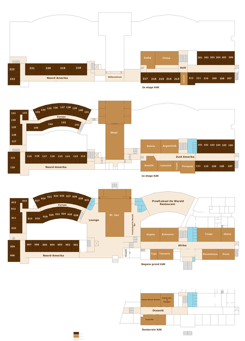
247 247