Modern Siege Weapons: Mechanics of the Trebuchet

Size: px

Start display at page:

Download "Modern Siege Weapons: Mechanics of the Trebuchet"

Kristopher Skinner
6 years ago
Views:

1 1/35 Modern Siege Weapons: Mechanics of the Trebuchet Shawn Rutan and Becky Wieczorek

2 The Project The purpose of this project is to study three simplifications of a trebuchet. We will analyze the motion over time of each of these models using differential equations and modern mechanics. 2/35

3 Why the Trebuchet? The trebuchet is a historical example of mechanics and the field of engineering. 3/35 The motion of a trebuchet can used as an example of a double and a triple pendulum. It s an awesome example of human ingenuity!

4 History of the Trebuchet The first trebuchets on record appear in Asia in the 7th century. They are rightly known as the heavy artillery of the middle ages. The chronicler Olaus Magnus writes of another trebuchet used at Kalmar. An old woman happened to sit down on the sling pouch and by mistake triggered the trebuchet with her walking stick. As a result she was hurled through the air across the streets of the town, apparently without suffering any damage. Another story about trebuchets is told by Froissart in connection with the siege of Auberoche in 1334 by the French. In this case an English messenger was captured and sent flying back to the castle with his letters tied around his neck. 4/35

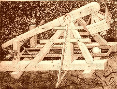
5 Various Historical Trebuchets 5/35

6 Lagrangian Mechanics Lagrangian mechanics is a way to analyze a system that is sometimes easier to use than Newtonian mechanics. What is the Lagrangian? The Lagrangian is defined as L = T V, where T is the kinetic energy and V is the potential energy of the system. Lagrangian mechanics utilizes an integral of the Lagrangian over time, called action. This path of minimum action will determine which of an infinite choice of paths a system or particle is likely to take. 6/35

The Euler-Lagrange Equation Derived from minimizing the action, the Euler-Lagrange equation gives us an simple way to solve for the equations of motion of a system.

7 The Euler-Lagrange Equation Derived from minimizing the action, the Euler-Lagrange equation gives us an simple way to solve for the equations of motion of a system. 7/35 The Euler-Lagrange equation depends on the degrees of freedom of the system (in how many ways can it move) The general Euler-Lagrange equation (as a function of the generalized coordinates of the system, q i ). L q i d dt ( ) L q i = 0 (1) There will be an equation for each degree of freedom, so our final model, which will be described as a function of θ, φ, and ψ, will require three equations.

8 The Ideal Launcher The counterweight falls the maximum distance allowable for any model All of the potential energy of the counterweight goes into kinetic energy of the projectile Projectile launched from the origin Launch angle of 45 8/35

9 The Seesaw Model m 1 (x 1, y 1 ) 9/35 l 1 (0, 0) θ l 2 (x 2, y 2 ) m 2 The seesaw model is an extreme simplification of the trebuchet The system can be modeled as a two mass pendulum. Only one degree of freedom, θ, means only one equation of motion.

10 Positions of the Masses The coordinates of m 1 are 10/35 x 1 = l 1 sin θ(t) and y 1 = l 1 cos θ(t). When we vectorize m 1, this becomes P 1 =< l 1 sin(θ), l 1 cos(θ) >. The coordinates of m 2 are x 2 = l 2 sin(θ) and y 2 = l 2 cos(θ) Similarly, the position vector describing the path of m 2, P 2, is defined as: P 2 =< l 2 sin(θ), l 2 cos(θ) >.

11 Energy of the System and the Lagrangian From the position functions, the kinetic and potential energies of each of the masses can be derived. Kinetic energy (T ) = 1 2 m v2, where v is the derivative of P Potential energy is given by the equation V = mg P y. Once you have the kinetic and potential energies, the Lagrangian is simple to calculate. L = 1 2 (m 1l m 2 l 2 2) θ 2 g cos(θ)( m 1 l 1 + m 2 l 2 ) = 1 2 (m 1l m 2 l 2 2) θ 2 + g cos(θ)(m 1 l 1 m 2 l 2 ) 11/35

12 Equations of Motion Applying the Euler-Lagrange equation to the Lagrangian gives us the equation L θ d ( ) L dt θ = 0 Solving this, we have our equation of motion to be 12/35 (m 1 l 1 m 2 l 2 )g sin(θ) (m 1 l m 2 l 2 2) θ = 0

13 13/35 Figure 1: A strobe-like image of the seesaw model in action

14 Range and Efficiency of the Seesaw Model The range is easily calculated from the x and y velocity of the projectile upon moment of release. Using the following parameters 14/35 θ(0) = 135, θ(0) = 0 g = 9.8m/s 2, l 1 = 10m, l 2 = 100m, m 1 = 1000 kg, m 2 = 1kg The range is calculated to be 2570 meters. Optimal release angle of Maximum range for a projectile shot by the ideal launcher is 34, 142 meters. This means the seesaw model is only 8% efficient.

15 Range(ft) / Angle(degrees) Figure 2: A graph of the release angle versus the range of the projectile

16 Trebuchet With a Hinged Counterweight (0, 0) θ l 1 φ l 4 m 1 (x 4, y 4 ) 16/35 l 2 (x 2, y 2 ) m 2 An example of a double pendulum More of the potential energy of the counterweight is translated into kinetic energy of the projectile This system is dependent on both θ and φ, so there will be two equations of motion.

17 Positions of the Masses The only change is the position of the counterweight This can be seen as a geometric addition of the original position vector for m 1 and a new position vector to the mass from that point. 17/35 Q 1 =< l 1 sin(θ) l 4 sin(θ + φ), l 1 cos(θ) + l 4 cos(θ + φ) > Q 2 =< l 2 sin(θ), l 2 cos(θ) >

18 The Lagrangian The Lagrangian of this system is dependent on both θ and φ. 18/35 L = T V = 1 2 m 1[l 2 1 θ 2 2l 1 l 4 θ( θ + φ)cos(θ) + l 2 4 ( θ + φ) 2 ] m 2l 2 2 θ 2 + m 1 gl 1 cos(θ) m 1 gl 4 cos(θ + φ) m 2 l 2 g cos(θ)

19 Equations of Motion We solve the ELE with respect to θ L θ d ( ) L dt θ = 0 From this we see that the first equation of motion is Eq1 = m 1 g sin(θ)l 1 + m 2 gl 2 sin(θ) + gm 1 l 4 cos(θ) sin(φ) + gm 1 l 4 sin(θ) cos(φ) m 1 l 2 1 θ + 2 θ cos(φ)m 1 l 4 l 1 2 θ sin(φ) φm 1 l 4 l 1 m 1 l 4 l 1 sin(φ)( φ) 2 + m 1 l 4 l 1 cos(φ) φ m 2 l 2 2 θ m 1 l 2 4 θ m 1 l 2 4 φ Solving the ELE with respect to φ L φ d dt ( L φ ) = 0 (2) 19/35

20 Thus, the second equation of motion is Eq2 = m 1 l 4 ( l 1 ( θ) 2 sin(φ) sin(φ) cos(θ)g g sin(θ) cos(φ) l 1 θ cos(φ) + l4 θ + l4 φ) (3) 20/35

21 21/35 Figure 3: A strobe-like image of the hinged counterweight trebuchet in action

22 Range and Efficiency We used the following parameters in our calculations. 22/35 θ(0) = 135, θ(0) = 0 φ(0) = 45, φ(0) = 0 g = 9.8, l 1 = 10, l 2 = 100, l 4 = 21, m 1 = 1000m 2 = 1

23 Range(ft) / Angle(degrees) Figure 4: A graph of the release angle versus the range of the projectile

24 Properties of the Hinged Counterweight Model Angular speed of this model is greater Optimal angle of release is 19. Maximum range of 16, 050 meters (approximately six times the range of the seesaw model) Range efficiency is 47% 24/35

25 Trebuchet with a Hinged Counterweight and Sling 25/35 (0, 0) θ l 1 φ l 4 m 1 (x 4, y 4 ) l 2 ψ l 3 (x 3, y 3 ) m 2

26 Benefits of the Sling Increase in the length of the throwing arm Rotational energy of the system is greater Angular velocity of the projectile is greater The overall range is increased 26/35

27 Positions of the Masses The position of m 1 is 27/35 R 1 =< l 1 sin(θ) l 4 sin(θ + φ), l 1 cos(θ) + l 4 cos(θ + φ) >. However, the position of m 2 has changed. Now, the new position of m 2 is R 2 =< l 2 sin(θ) l 3 sin( θ + ψ), l 2 cos(θ) l 3 cos( θ + ψ) >.

28 The Lagrangian 28/35 L = 1 2 ( θ) 2 m 1 l 2 1 m 1 l 4 l 1 ( θ) 2 cos(φ) + m 1 gl 1 cos(θ) m 1 l 4 l 1 θ φ cos(φ) ( θ) 2 m 2 l 2 2 m 2 gl 2 cos(θ) m 2 l 3 l 2 ( θ) 2 cos(ψ) + m 2 l 3 l 2 θ ψ cos(ψ) m 2l 2 3( ψ) 2 m 2 l 2 3 θ ψ m 2l 2 3( θ) 2 + m 2 gl 3 cos( θ + ψ) + m 1 l 2 4 θ φ m 1l 2 4( φ) m 1l 2 4( θ) 2 gm 1 l 4 cos(θ + φ)

29 Equations of Motion We solve the ELE with respect to θ L θ d ( ) L dt θ = 0 29/35

30 From this we see that the first equation of motion is Eq1 = m 1 gl 1 sin(θ) + m 2 gl 2 sin(θ) m 2 gl 3 sin(θ) cos(ψ) + m 2 gl 3 cos(θ) sin(ψ) + m 1 gl 4 sin(θ) cos(φ) + m 1 gl 4 cos(θ) sin(φ) θm 1 l m 1 l 4 l 1 θ cos(φ) 2m 1 l 4 l 1 θ sin(φ) φ + m1 l 4 l 1 φ cos(φ) m 1 l 4 l 1 ( φ) 2 sin(φ) θm 2 l m 1 l 3 l 2 θ cos(ψ) 2m2 l 3 l 2 θ sin(ψ) ψ m 2 l 3 l 2 ψ cos(ψ) + m2 l 3 l 2 ( ψ) 2 sin(ψ) + m 2 l 2 3 ψ m 2 l 2 3 θ m 1 l 2 4 φ m 1 l 2 4 θ Solving the ELE with respect to φ L φ d dt ( L φ ) = 0 (4) 30/35

31 Thus, the second equation of motion is Eq2 =m 2 l 3 l 2 ( θ) 2 sin(ψ) m 2 gl 3 cos(θ) sin(ψ) + m 2 gl 3 sin(θ) cos(ψ) m 2 l 3 l 2 θ cos(ψ) m2 l 2 3 ψ + m 2 l 2 3 θ Solving the ELE with respect to ψ L ψ d dt ( L ψ ) = 0 Thus the third equation of motion is Eq3 =m 1 l 4 l 1 ( θ) 2 sin(φ) + m 1 gl 4 cos(θ) sin(φ) + m 1 gl 4 sin(θ) cos(φ) + m 1 l 4 l 1 θ cos(φ) m1 l 2 4 θ m 1 l 2 4 φ (5) (6) 31/35

32 32/35 Figure 5: A strobe-like image of a trebuchet with a hinged counterweight and sling

33 Range and Efficiency Optimal θ angle of release is 2.7. Optimal ψ angle of release is Maximum range is 29, 030 meters (approximately twice the range of the trebuchet with just a hinged counterweight and approximately fourteen times the range of the seesaw trebuchet). Range efficiency is 84% for this trebuchet model. Only 16% shy of being a perfect launcher! 33/35

34 Range(ft) / Angle(degrees) Figure 6: Release Angle (θ) vs. Range

35 Conclusion The trebuchet was developed before the methods of calculus were discovered. It was the most destructive weapon of its day due to its efficient use of energy and great range. The abilities of the trebuchet still spark the interest of both historians and engineers. Although the development of the trebuchet took hundreds of years, today we can use mathematical modeling to reproduce these advancements in hours. 35/35

Modeling of a Trebuchet with a Sling and Counterweight

Modeling of a Trebuchet with a Sling and Counterweight MEAM 211 Project 3, Phase III April 4, 2007 Background In Phase III, you are required to analyze the dynamics of a trebuchet with a sling and develop