Interglacials of the last 800,000 years Authorship: Past Interglacials Working Group of PAGES (list of contributors at end)

Transcription

1 Interglacials of the last 800,000 years Authorship: Past Interglacials Working Group of PAGES (list of contributors at end) Corresponding author: Eric Wolff, Key points We have reviewed the occurrence, strength, shape and timing of interglacials Despite spatial variability, MIS 5 and 11 stand out as strong/warm The current interglacial is expected to be longer than any of those reviewed Index terms: 4936 (Interglacials), 4946 (Milankovitch cycles), 0473 (Paleoclimatology and paleoceanography), 1622 (Earth system models), 1105 (Geochronology). This article has been accepted for publication and undergone full peer review but has not been through the copyediting, typesetting, pagination and proofreading process which may lead to differences between this version and the Version of Record. Please cite this article as doi: /2015RG

2 Abstract Interglacials, including the present (Holocene) period, are warm, low land-ice extent (high sea level), end members of glacial cycles. Based on a sea-level definition, we identify eleven interglacials in the last 800,000 years, a result that is robust to alternative definitions. Data compilations suggest that, despite spatial heterogeneity, Marine Isotope Stages (MIS) 5e (last interglacial) and 11c (~400 ka ago) were globally strong (warm), while MIS 13a (~500 ka ago) was cool at many locations. A step change in strength of interglacials at 450 ka is apparent only in atmospheric CO 2, and in Antarctic and deep ocean temperature. The onset of an interglacial (glacial termination) seems to require a reducing precession parameter (increasing northern hemisphere summer insolation), but this condition alone is insufficient. Terminations involve rapid, non-linear, reactions of ice volume, CO 2 and temperature to external astronomical forcing. The precise timing of events may be modulated by millennialscale climate change that can lead to a contrasting timing of maximum interglacial intensity in each hemisphere. A variety of temporal trends is observed, such that maxima in the main records are observed either early or late in different interglacials. The end of an interglacial (glacial inception) is a slower process involving a global sequence of changes. Interglacials have been typically ka long. The combination of minimal reduction in northern summer insolation over the next few orbital cycles, owing to low eccentricity, and high atmospheric greenhouse gas concentrations implies that the next glacial inception is many tens of millennia in the future. 2

3 1. Introduction interglacials of the last 800 ka Earth s climate of the last 800 ka (1 ka = 1000 years) is the latest stage in a slow cooling that has been in progress for the last ~50 Ma (1 Ma = one million years) [Zachos et al., 2008]. During this cooling, ice sheets formed on the Antarctic continent ~40 Ma ago, while the first signs of northern hemisphere (NH) glaciation appeared much more recently. Only at the start of the Quaternary Period and the Pleistocene Epoch, ~2.6 Ma ago, did alternations between cold glacial periods with ice on the NH continents, and warmer intervals with little or no NH continental ice, first appear, reflected in the appearance of ice-rafted debris [Shackleton et al., 1984; Kleiven et al., 2002] and in enhanced amplitude of cyclicity in benthic oxygen isotopes in marine sediment records (Figure 1) [Lisiecki and Raymo, 2005]. Somewhere between 1.2 and 0.6 Ma ago, weaker cycles with a period of ~40 ka gave way to stronger (greater isotopic amplitude) cycles with a recurrence period closer to 100 ka. This change is known as the Mid-Pleistocene Transition or Revolution. Its exact date is debated, and it is likely that different aspects of climate shifted into their new mode of operation at different times [Mudelsee and Schulz, 1997; Rutherford and D'Hondt, 2000; Clark et al., 2006; Elderfield et al., 2012]. By 800 ka ago, the change in amplitude was complete in most records, and glacial cycles with sea level amplitudes of more than 100 m were occurring, mostly with lengths of the order of 100 ka. The last 800 ka time period also benefits from the enormous progress over recent decades in collecting and analyzing a wide range of continuous climate records from terrestrial sites, marine sediment cores, and the oldest Antarctic ice cores. It is approximately the most recent interval associated with the orientation of the Earth s magnetic field in the normal polarity with the inclination vector pointing north [Shackleton et al., 1990], providing a useful sedimentary demarcation in settings where magnetic reversals are preserved. As an additional motivation, it has also become possible in recent years to run Earth models of intermediate complexity (EMICs) through several glacial cycles, and full Earth system models (ESMs) for a significant range of boundary conditions, including those appropriate for some of the recent interglacials. Interglacials are the warm, low ice extent (high sea-level) end members of the glacial cycles although as we shall discuss, the exact definition of an interglacial is not simply stated. We live in such an interglacial. Human actions, increasing the concentration of greenhouse gases in the 3

4 atmosphere, ensure that our climate will become warmer in the next century, and remain warm for many millennia to come [IPCC, 2013]. This makes particularly pertinent the study of periods in which at least sectors of the Earth system may have been warmer than they are currently. Our understanding of the climate of our current interglacial is good in a static sense: given the boundary conditions (solar irradiance, astronomical characteristics, geography, ice cover, concentrations of long-lived greenhouse gases such as CO 2 ) and the resulting radiation balance of the planet. However, we cannot currently give a satisfactory explanation of how the climate system evolved to this state: why we live in an interglacial at this time, or indeed why we live in an interglacial embedded in 100 ka rather than 40 ka cycles. Finally the entries into interglacials (and exits from them) are fascinating examples of non-linear behavior of the Earth system that need to be understood. For these reasons importance of warm periods, need to understand how our current climate arose, fascinating climate dynamics, and recent availability of significant amounts of data and model simulations it is timely to review and synthesize existing knowledge about the warm periods (interglacials) of the last 800 ka. After identifying what an interglacial is, this review aims to summarize the common features and differences between them. This allows us to highlight particular interglacials that may enlighten us about the climate system, and to describe current knowledge of the factors that lead into and out of an interglacial. The review ends with a discussion about the likely extent of the present interglacial, both in the absence and presence of human influence on the climate system. 2. Identifying interglacials 2.1. Nomenclature and history Terrestrial, marine and ice core sequences deposited since the intensification of NH glaciation, ~2.6 Ma ago have traditionally been divided on the basis of climate changes inferred from their lithological, biological and geochemical signature. The fundamental units of this geologic-climate classification [American Commission on Stratigraphic Nomenclature, 1961] are (i) glaciations (or glacials), representing episodes during which extensive glaciers developed; and (ii) interglaciations (or interglacials), representing episodes during which the climate was incompatible with the wide 4

5 extent of glaciers. Further subdivisions include stades (stadials) and interstades (interstadials), reflecting secondary advances and recessions or standstills of glaciers, respectively. The term interglacial derives from the position of temperate-climate sediments interbedded between glacial sediments [Heer, 1865; Geikie, 1874]. In the higher mid-latitudes of Europe and North America the concept of an interglacial as an interval of time during which conditions were at least as warm as the present interglacial (Holocene) was traditionally based on floral evidence, indicating the development of temperate deciduous forest [e.g., Jessen and Milthers, 1928; Fairbridge, 1972; Woillard, 1978; West, 1984; Gibbard and West, 2000]. By comparison, the term interstadial has been used to describe a period that was either too short or too cold to allow the development of temperate deciduous forest. Similar distinctions were also adopted for faunal evidence [e.g., Coope, 1977]. In deep-sea sediments, the terms glacial and interglacial were first applied to even- and oddnumbered oxygen isotope stages, respectively, defined by variations in the oxygen isotope ratio (δ 18 O) in planktonic foraminifera and first thought to reflect changes in sea surface temperature [Emiliani, 1955]. However, the concept of a marine isotopic stratigraphy is based on the principle that changes in the oxygen isotopic composition of the oceans primarily arises from changes in the volume of ice stored on the continents [Shackleton, 1967] and that, given the slow mixing of the deep ocean, such a signal would be global on timescales of thousands of years. Shackleton and Opdyke [1973] proposed the formalization of Marine Isotope Stages (MIS) 1-22, using the δ 18 O in foraminifera in core V from the Eastern Equatorial Pacific, a practice which has been gradually extended over the entire Pleistocene, Pliocene and beyond. Marine isotope stages may be further divided into substages (e.g., MIS 5 into 5a-e [Shackleton, 1969]), characterized by local minima and maxima in δ 18 O values known as marine isotopic events [Prell et al., 1986], such that MIS 5a contains event 5.1, MIS 5b contains event 5.2 and so on. The decimal event notation has occasionally been used to denote substages, but the two systems are not interchangeable. An event refers to a point in time rather than an interval; in a detailed record there will be space between successive events, whereas substages have boundaries and together fill the stratigraphic record and the time that it represents [Shackleton, 2006]. To avoid confusion, please note that we use a recently recommended substage nomenclature [Railsback et al., 2015], which contrasts with some literature usage, particularly for MIS 9 and MIS 15. 5

6 A major development in the understanding of the correspondence between marine and terrestrial stages was the realization that the Eemian (Last) Interglacial of northwest Europe is not equivalent to the whole of MIS 5, but rather approximates to a substage (MIS 5e) within it [Shackleton, 1969]. In line with the terrestrial evidence, other isotopically depleted marine substages corresponded to interstadials associated with the same interglacial complex (so that MIS 5c and 5a would broadly correspond to the Amersfoort/Brörup and Odderade interstadials, respectively, of the northwest European stratigraphy). Joint foraminiferal isotopic and pollen analyses from marine sequences have confirmed such correlations, but also showed that the marine and terrestrial stage boundaries are not necessarily time parallel, reflecting geographical asynchroneity, and differences in response times of e.g., vegetation and ice [Sánchez Goñi et al., 1999; Shackleton et al., 2002; Shackleton et al., 2003; Tzedakis et al., 2004] Definition of interglacial The population of interglacials must be defined before any attempt is made to discuss their individual characteristics, including the statistics of their timing and spacing. Given that interglacial complexes (odd-numbered Marine Isotope Stages, such as MIS 5, but excluding MIS3 which is not now considered to include an interglacial period) contain a number of temperate intervals within them, a crucial question is how to categorize interglacials and distinguish them from interstadials. In some conceptual models [Parrenin and Paillard, 2003], the climate system occupies (and jumps between) a glacial and deglacial (or interglacial) state, with different governing equations in each. While a bifurcation structure may indeed be relevant for describing the dynamics of glacialinterglacial cycles, identifying it from the available palaeo-observations is complex [Imbrie et al., 2011]. Distinguishing interglacial from interstadial climates is nonetheless important, not only on formal stratigraphic grounds, but also in climatic context. Though temperate in climatic signature, interstadials are still part of a glacial world with excess ice in the Northern Hemisphere outside Greenland. Thus, for example, the Amersfoort/Brörup and Odderade interstadials in northwestern European nomenclature (roughly MIS 5a and 5c) are part of the Early Glacial (MIS 5d-5a) in this region, which reflects not only their stratigraphic position, but also their overall climatic character compared to the Eemian. 6

7 Central to any definition of an interglacial is the choice of an appropriate criterion that can be applied consistently through time. A number of approaches are possible, each with inherent advantages and disadvantages (Table 1). A recurring issue is that distinctions between interglacials and interstadials depend on the metric used. It is desirable that whatever metric is chosen has global significance, such that interglacials are phenomena that can be considered widespread (probably of global extent), even if their regional expression is neither globally uniform or synchronous. Some definitions that have been used are based on temperature. Temperature records exist at many sites, but are essentially local, and therefore the definition of an interglacial based on temperature would vary according to the location. This will remain the case until there are sufficient data with accurate chronologies, such that some kind of global average temperature can be constructed across multiple glacial/interglacial cycles. Only recently has a first such reconstruction [Shakun et al., 2012; Marcott et al., 2013] become available for the last 22 ka, and none is available for earlier interglacials. We might also be tempted to define interglacials on the basis of the external forcing. At the multimillennial time scale, the dominant external forcing of Earth s climate is the astronomical forcing. This drives the climate system dynamics which, lead, for example, to variations in atmospheric CO 2 concentration and in the mass of the ice sheets. These in turn may be viewed as feedbacks, or as internal forcing factors of the atmospheric and oceanic conditions all over the globe. Increased concentrations of CO 2, in particular, are a characteristic of interglacials. However, the relationships between astronomical forcing, CO 2 and the mass of continental ice are non-linear and complex. In particular, eccentricity, often cited as a possible origin of the 100-ka periodicity characteristic of glacial-interglacial cycles does not appear in the spectrum of regional insolation changes; it merely modulates the amplitude of insolation changes. Combinations of obliquity and precession predict the occurrence of some interglacials [Kukla et al., 1981], but as longer paleoclimate records have appeared, it has become clear that such simple formulae do not correctly predict the full roster observed in the data. It is therefore not currently practical to use astronomical forcing to define interglacials. As discussed earlier, interglacials have been defined as episodes during which global climate was incompatible with the wide extent of glaciers [American Commission on Stratigraphic Nomenclature, 1961]. While remembering that there is still a large volume of ice in Antarctica 7

8 during every interglacial, this nonetheless emphasises that the fundamental concept underlying the terminology of an interglacial is that of low continental ice volume, a consequence of integrated global climate effects, which would also be observed as high sea-level or less positive seawater δ 18 O. This is in line with early definitions of interglacials based on the marine transgression [e.g., Harting, 1874]. The slow response of ice sheets would mean that the sea level highstand or isotopic minimum may be attained relatively late compared to increases in warmth or climate forcing. Here we clearly distinguish the use of such values to define whether an interglacial is occurring, from any measure used to define when the interglacial starts and ends. As an example, for the current interglacial, sea level close to present, a value we might use to define MIS 1 as an interglacial, occurs as late as~7-8 ka ago. However, having determined that an interglacial is occurring, its start can be defined in other ways [Walker et al., 2009]. A eustatic, or global mean, sea-level curve would therefore provide a useful measure to address this issue, but in practice direct sea-level determinations are often complicated by local isostatic and gravitational effects and dating uncertainties, are discontinuous, and only cover the most recent part of the record [e.g., Thompson and Goldstein, 2006]. The δ 18 O from benthic foraminifera is sometimes used as a sea-level proxy, but it is overprinted by local deep-water temperature and hydrographic effects, which can obscure the glacioeustatic signal [Chappell and Shackleton, 1986; Skinner and Shackleton, 2005]; averaging many globally distributed δ 18 O benthic records as in the stacked record of Lisiecki and Raymo [2005] (hereafter referred to as LR04) does however remove some of the regional variability. Various approaches to isolate the sea-level component of δ 18 O benthic [Shackleton, 1987; McManus et al., 1999; Shackleton, 2000; Waelbroeck et al., 2002] have been attempted, but until recently none of them have been extended to cover the last 800 ka. A modelled sea-level curve by Bintanja and van de Wal [2008] extends over the last 3 million years, but depends on uncertain assumptions about deep-water temperatures and their coupling with atmospheric temperatures. A record using shallow-infaunal benthic foraminifera to deconvolve deep-water temperatures (using Mg/Ca ratios) and the δ 18 O of seawater (δ 18 O sw ) over the last 1.5 million years has recently become available from ODP site 1123 on the Chatham Rise, east of New Zealand [Elderfield et al., 2012]. With hydrographic effects considered minimal at this site, the δ 18 O sw provides an important insight into ice-volume changes over this interval, although the propagated error of ±0.2 in calculated δ 18 O sw estimated by Elderfield et al. [2012] means that the 8

9 uncertainty is ±20 m sea-level-equivalent. A continuous sea-level reconstruction based on planktonic δ 18 O records and a hydrological model for the Red Sea is available for the last 520 ka [Rohling et al., 2009]. A related method covering a longer time period, using a hydrological model for the Mediterranean [Rohling et al., 2014], gives a further useful overview, but with a large propagated uncertainty in sea level, similar to that of Elderfield et al. [2012]. Finally, recent work [Shakun et al., 2015] has used a global compilation of paired planktonic δ 18 O and sea surface temperatures in an attempt to deduce δ 18 O of surface seawater, interpreted to reflect mainly ice volume and sea level. However, it is hard to use this record to compare the strength of interglacials because the authors had to make a correction for a long-term trend, believed to be unrelated to sea level. Given that the LR04 stack is affected by deep-water temperature and hydrographic effects of variable influence through time, we first examine those records where the sea-level component has been (mostly) isolated. The ODP Site 1123 [Elderfield et al., 2012], the Red Sea/Mediterranean [Rohling et al., 2009; Rohling et al., 2014], and the detrended surface seawater stack [Shakun et al., 2015] records all suggest that, within the uncertainties of the reconstructions (±20 m), highstands during the most prominent isotopic substages of the last 800 ka reached a level similar to present (Figure 2). Assuming that the East Antarctic ice sheet was not significantly smaller than today, this observation points to a more specific definition of an interglacial as an interval within which the distribution of northern hemisphere ice resembled the present (0±20 m), i.e., there was little northern hemisphere ice outside Greenland, with periods of significantly greater ice volume (sea level passing below approximately -50 m compared to present) before and after the interglacial period. The second half of the definition is required in order to separate periods of interglacial character that are interrupted by clearly glacial conditions. However it has consequences for the number of interglacials in MIS 15 and 7. The distinction between an interglacial and an interstadial under this definition lies in the absence/presence of significant northern hemisphere ice outside Greenland. An example of this distinction is MIS 5. Evidence from the Norwegian Sea and western Scandinavia indicates ice-free conditions during the Eemian (interglacial), but expansion of mountain glaciers during the Amersfoort/Brørup (MIS 5c) and Odderade (MIS 5a) interstadials leading to increased background values in the relative abundance of ice-rafted detritus in the Norwegian Sea during these intervals [Baumann et al., 1995]. 9

10 Tzedakis et al. [2009] assigned an interglacial status to the most prominent temperate (low δ 18 O) interval within each odd-numbered marine isotope stage of the LR04 benthic δ 18 O stack [Lisiecki and Raymo, 2005] (with the exception of the historical artifact of MIS 3). On this basis, MIS 5e, 9e, 11c, 13a, 17c, 19c (and by default MIS 1) are unambiguously the most prominent intervals within each MIS (Figure 2), but choosing the most prominent interval in MIS 7 and MIS 15 is difficult. Yin and Berger [2010; 2012] chose a similar set of interglacials to simulate, using the expectation of a 100 ka cycle to justify including MIS 7e but not 7a-c, and including MIS 15a but not 15e. Using our sea level definition, MIS 7a-c and 7e, and also MIS 15a and 15e are all equally prominent within their respective stages, and as we do not assume a particular periodicity, they are all included in our interglacial roster, which therefore comprises MIS 1, 5e, 7a-7c (as a single interglacial), 7e, 9e, 11c, 13a, 15a, 15e, 17c, 19c. Although a definition based on sea level, as we have suggested, is attractive in its simplicity, its application is hampered by uncertainties that remain in the values of sea level provided by indirect but continuous methods. In particular, direct sea level evidence suggests [Dutton and Lambeck, 2012; Kopp et al., 2013] that sea level during MIS 5e was higher than present. However, the (ODP 1123) derived sea level record [Elderfield et al., 2012] places the MIS 5e highstand at the edge of the lowest range of our proposed threshold (-20 m), and at a similar level in MIS 5a, with MIS 5c higher than both (Figure 2). Had we only the ODP1123 data [Elderfield et al., 2012], then MIS 5a and MIS 5c would have been identified as interglacials on a par with MIS 5e, but we use knowledge from other sea level datasets [Dutton and Lambeck, 2012; Grant et al., 2012; Kopp et al., 2013] to distinguish MIS 5e as an interglacial and MIS 5a and 5c as interstadials. This however casts doubt on the reliability of the reconstruction in earlier periods (especially before 450 ka ago) when alternative sea level evidence is weaker. Given this uncertainty, we also test the sensitivity of our interglacial assignments by using simple thresholds in the uncorrected benthic oxygen isotope record (in this case the LR04 stack [Lisiecki and Raymo, 2005]), and in the ice core record of CO 2 (chosen as a global-scale indicator which, together with ice volume/extent, affects the global radiative forcing). Our sensitivity studies with the LR04 benthic isotope stack [Lisiecki and Raymo, 2005] would produce the same set of interglacials for any threshold between 3.5 and 3.73 (to qualify as an interglacial, values lower than the threshold must be achieved). Any threshold set lower than

11 would exclude first MIS 17c and very quickly all other stages except MIS 1, 5e, 9e and 11c. At thresholds higher than 3.73, several other stages, starting with MIS 5c, would become interglacials. The very wide range of thresholds ( ) that lead to the same answer suggest that this solution is robust, i.e., that new data are unlikely to make it obsolete. We need also to assess the criterion for how deep the surrounding glacials must be to decide that a peak qualifies as a separate interglacial. Using LR04, it would in theory be possible to set a second threshold for the depth of the valley between interglacials, such that MIS 13 and 15 are separate interglacials, while MIS 7a-e and MIS 15a-e each form single very long interglacials. However, the range of values for such a second threshold is very narrow (~0.1 ), suggesting that it has no robust validity. In addition it would imply inclusion in an interglacial of isotopic values (during MIS 7d and 15b) that are generally characteristic of periods that are clearly part of the glacial world. A final argument against this solution is that two of the derived sea level records [Elderfield et al., 2012; Shakun et al., 2015] place sea level lower in MIS 7d than in MIS 14. Thus, unless we are willing to describe MIS as a very long continuous interglacial, we are forced to set the threshold such that MIS 7ac and 7e (similarly 15a and 15e) are separate interglacials. As a final sensitivity study, we investigate the ice core CO 2 record [Lüthi et al., 2008; Bereiter et al., 2015]; because of its importance as a radiative forcer at global scale, CO 2 may plausibly be one of the controlling factors on interglacial strength in a range of other records (see section 6.7). If the threshold is 260 ppm or higher, only one interglacial (MIS 19) is recognized before MIS 11. However, as the threshold is lowered other interglacials qualify: by 250 ppm, all the interglacials in our roster (including 7c and 15a) have qualified, with the exception of MIS 17c. Periods of clearly interstadial nature in other records get drawn in for lower thresholds, starting with MIS 5a. The low values of CO 2 in MIS 17c were already noted [Lüthi et al., 2008]and persist even in the revised dataset recently published [Bereiter et al., 2015]. Perhaps most importantly for this sensitivity study, there is again no reasonable criterion using CO 2 that qualifies MIS 13a as an interglacial without also qualifying MIS 7c and 15a as separate interglacials. The scheme we have used allows for the occurrence of more than one interglacial within the same complex and does not require an interglacial to follow a traditionally-numbered glacial termination. Only a definition that insists on a minimum temporal spacing (of order 100 ka) between 11

12 interglacials could force a more traditional list of interglacials. While we recognize that the definition applied here will lead to some inconsistency in relation to traditional nomenclature, we feel it is justified by its objectivity and robustness against a range of definitions and thresholds; the traditional assumptions on the other hand will lead to misleading conclusions about the spacing and timing of interglacials. It is important to reiterate that this is a working definition based on a global metric and as such it has global stratigraphic significance. Interglacial stages may continue to be defined in local contexts using local signals (e.g., local temperature or forest development), but they do not carry general applicability. One cautionary note to add is that our definition is clearly dependent on the context of the last 800 ka, and would not necessarily be suitable for the early Quaternary, even though we recognise from benthic isotopes that periods with interglacial character existed then, nor for earlier periods containing alternations of icy and ice-free intervals. 3. Methods Before attempting to assess the nature, intensity and timing of interglacials, it is necessary to establish and summarize the main methods used to measure interglacial climate characteristics, to place them on an age scale, and to model the processes involved Stratigraphy and Chronology Regardless of what definition is adopted for an interglacial, the study of past interglacials must be underpinned by a robust stratigraphy and chronology. Comparing climate signals in different archives is challenging and requires precise stratigraphic correlation of marine, ice, and terrestrial records, including those providing information about sea level and atmospheric composition. Study of the initiation, termination, and duration of interglacials as well as rates of processes is entirely dependent on the accuracy of the time scale. The age model controls the rate, shape, and duration of interglacial periods and absolute ages are needed to discuss the phasing of proxies relative to astronomical forcing. Sampling frequency as well as chronological precision can affect the degree of variability and peak values (amplitude) of the interglacial signal. The long ice core records have relied mostly on the Antarctic Ice Core Chronology 2012 (AICC 2012) based on information from several ice cores [Bazin et al., 2013], and its predecessor, the EDC3 chronology that was derived by inversion of a snow accumulation and mechanical ice flow 12

13 model using a set of independently dated horizons (age markers) along the core [Parrenin et al., 2007]. Note that all ages shown in figures in this paper are nominally relative to 1950 as present. The uncertainty of the EDC3 (EPICA Dome C, 3 rd generation) age model is estimated to be ±3 ka at 100 ka ago and increasing to ±6 ka from 130 ka to the base of the core. AICC2012 [Bazin et al., 2013] shows only small differences from EDC3 and is well within the quoted age uncertainty. The duration of the last four interglacial periods is not affected by more than 5 % using AICC2012 instead of EDC3 [Bazin et al., 2013]. One powerful alternative method for developing ice core chronologies is orbital tuning of the O 2 /N 2 ratio to local insolation forcing [Bender, 2002; Kawamura et al., 2007]. This method has the advantage that it dates the ice (which holds the climate signal), rather than the enclosed air, which can be considerably younger because the air bubbles close only at depths of typically m). With an assumption that O 2 /N 2 is in phase with local summer insolation, this method provides a link to absolute ages however, the precision of this assumption has been questioned [Landais et al., 2012]. Vostok O 2 /N 2 data are included in AICC2012 as one component of the age model, but the Dome Fuji (DFO2006) age model relies mainly on this tuning, and a smaller estimated uncertainty (up to 2.5 ka) is quoted. Comparison of EDC3 and Dome Fuji chronologies reveals reasonable agreement for the last 350 ka (within the estimated uncertainty of EDC3, but not always within the uncertainty quoted for DFO2006). Most deep-sea records are dated by correlating benthic δ 18 O signals to the LR04 stack [Lisiecki and Raymo, 2005]. The LR04 stack is tuned to the output of an ice volume model [Imbrie and Imbrie, 1980] that, in turn, is driven by insolation, assuming fixed response times. The estimated error for LR04 is ±4 ka for the past million years. One of the caveats associated with the LR04 time scale is its reliance on assumptions associated with astronomical forcing of climate. The depth-derived ages of Huybers and Wunsch [2004] are almost free of such assumptions but are estimated to be accurate only to within ±9 ka. The differences between LR04 and other age models fall within the uncertainties of these error estimates (Figure 3). LR04 and EDC3 or AICC2012 are well aligned with each other although Antarctic temperature changes consistently lead LR04 δ 18 O by an average of 3 ka. The deep-sea temperature component of the benthic δ 18 O signal, as estimated by Mg/Ca, significantly leads the δ 18 O seawater signal [Elderfield et al., 2012] (see discussion below) and agrees closely with the timing of Antarctic temperature change (Figure 3). This likely reflects the late response of ice volume compared to 13

14 temperature in the benthic δ 18 O signal. The lead of warming Antarctic and deep-sea temperatures over (NH) ice volume change underscores the problem of how to define the start of interglacial periods because the early warming may not be considered to be part of the interglacial period if defined by ice volume reduction. Speleothems and corals provide an opportunity for absolute dating of the timing of terminations [e.g., Cheng et al., 2009] and the duration of interglacials by radiometric U series dating, and to determine the phasing of climate change relative to insolation forcing. If age markers from speleothems can be identified as unequivocally synchronous to features in ice cores and/or marine sediment cores, then the speleothem chronology can be exported to other archives [e.g., Barker et al., 2011; Grant et al., 2012] and used to evaluate the accuracy of independent chronologies. Full use of such methods awaits firm proof that rapid jumps in local speleothem δ 18 O are synchronous with rapid jumps in ice core temperature or atmospheric methane and marine sea surface temperature (SST) records. Assumptions of this nature have been disputed [e.g., Blaauw et al., 2010]. Barker et al. [2011] placed the EPICA Dome C (EDC) record on a Speleo-Age timescale for the last 400 ka by first differentiating the Antarctic δd record, according to a conceptual model of interhemispheric millennial temperature change, to produce a synthetic Greenland record, and then correlating cold events in Greenland with weak monsoon events in the detrended speleothem δ 18 O record. The ages agree to within ±2-3 ka with EDC3 from present to MIS 11 where the difference increases to 5 ka. A similar approach has been applied to Iberian Margin sediments where planktonic δ 18 O and SST have been used to synchronize millennial-scale events among marine sediment core, Antarctic ice core, and speleothem records [Barker et al., 2011; Hodell et al., 2013]. Differences between the speleo-synchronized and LR04 age models from the Iberian Margin are less than ±5 ka for the last 400 ka. While speleothem records can be radiometrically dated, the age models of other long terrestrial records have been derived by tuning litho- or bio-stratigraphical variations to an astronomical target (which may be a local insolation target) or to marine records [Prokopenko et al., 2006; Tzedakis et al., 2006; Melles et al., 2012; Torres et al., 2013]. While this can be done rather precisely, it involves assumptions about synchroneity that could be in error by several thousand years. Unless these assumptions can be tested (for example through the use of pollen in marine cores, of tephra layers that can be shown to have the same origin, or through the use of dated paleomagnetic 14

15 boundaries), it is impossible to assess the phasing of change between different processes during relatively rapid changes that occur at terminations in particular. The accuracy of time scales directly influences our interpretations of the causes of interglacial periods. For example, the errors associated with the ages for the onset and end of an interglacial period (regardless of defining criteria) are large relative to the accuracy of astronomical solutions, which we take to have no error for the last 800 ka. The absolute chronological error (of order ±5 ka for ice cores and marine records) is also large relative to the duration of interglacial periods, which ranges from ~10 to 30 ka. The age uncertainty (about one quarter of a precession cycle) provides considerable leeway in interpretation of how the onset and end of interglacials align with astronomical forcing, underscoring the importance of reducing chronological error in the future Proxies Temperature, greenhouse gas (GHG) concentrations, and ice volume (sea level) have been the three reconstructed climate parameters used most often for studying past interglacial periods, although changes in the hydrologic cycle are also important especially at low latitudes, and changes in ocean circulation are also highly relevant. Clearly it is not appropriate here to review all the methods used in palaeoclimate reconstruction; however, we briefly summarize the main methods used to derive the records that appear most often in this paper. In the polar regions, temperature is derived from the ratios of water isotopes (δ 18 O, δd) in ice cores. This has a strong physical basis as a temperature proxy [Jouzel et al., 1997], but there remains uncertainty about its calibration, particularly for higher temperatures [Sime et al., 2009]. Additional methods to constrain temperature in ice cores have been used [e.g., Buizert et al., 2014] in Greenland ice cores, but so far the water isotopes are the only method used to reconstruct temperatures in the long Antarctic ice cores that extend through several glacial cycles. SSTs are estimated from marine sediment cores using a range of geochemical and biological proxies: fossil assemblages (using foraminifera, coccolithophores, radiolarians, diatoms or dinocysts), alkenone and other biomarkers (U k 37, U k 37, TEX 86 ), Mg/Ca ratios and clumped isotopologues of carbon and oxygen. Each of these methods comes with uncertainty about calibration and about the precise interpretation of the proxy (for example whether it indicates an annual or seasonal signal). Where methods have been compared, discrepancies are found in some regions [Nurnberg et al., 2000; de 15

16 Vernal et al., 2006; de Garidel-Thoron et al., 2007]. This means that it is difficult to construct consistent spatial timeslices of absolute temperature. However, the relative signal within a single proxy at a single site should be much more reliable, so that anomaly data can be used with some confidence to assess the relative strength of different interglacials, or the timing of maxima and transitions at a given location. For terrestrial sites, pollen assemblages may sometimes be used to estimate temperature; many other commonly-described terrestrial proxies are influenced by factors other than temperature. GHG concentrations (particularly CO 2, CH 4 ) for the last 800 ka can be determined directly from measurements in the air within ice cores [e.g., Loulergue et al., 2008; Lüthi et al., 2008]. The uncertainty in the concentrations measured in this way is very small (a few ppm for CO 2 and about 10 ppb for CH 4 ), although methodology is important for obtaining correct values, especially in deep ice [Bereiter et al., 2015]. However, in the cores for which old ice is available, there is an inherent limit to the resolution (of several centuries), and an uncertainty in the age relative to the temperature proxy in the same core, because of changes in delta-age, the age difference between the ice and the younger air that diffuses from the surface and is trapped within the ice matrix only at depth [e.g., Parrenin et al., 2013]. CH 4 changes result from changes in wetlands in the tropics and high northern latitudes, and thus are often used as an indicator in the gas phase of the timing of northern hemisphere and tropical climate change relative to other signals. Estimates of relative sea level change at individual sites and dates can be made using a range of methods (already partly discussed in section 2.2). While dated corals are of particular importance, to obtain a continuous (over multiple glacial cycles) and global, eustatic, sea level record, marine sediments remain important. The δ 18 O of benthic foraminifera is affected by changes in continental ice volume, but also by deep-water temperature and local hydrographic (water mass) changes. On timescales significantly greater than the mixing time of the oceans (10 3 yrs), the δ 18 O calcite signal represents changes in the mean state of the global ocean as local/regional hydrographic changes that exist in the ocean are diminished [Shackleton, 1967; Imbrie et al., 1984; Skinner and Shackleton, 2006]. If an independent estimate of temperature is derived, the seawater δ 18 O component (i.e., δ 18 O seawater ) of the benthic δ 18 O signal can be calculated. As discussed in section 2.2, one approach has been to stack benthic δ 18 O records assuming that local and regional hydrographic signals are averaged out, thereby leaving the common global δ 18 O signal [Imbrie et 16

17 al., 1984; Prell et al., 1986; Lisiecki and Raymo, 2005]. In reality, however, the relative contributions of temperature and ice volume still remain unconstrained in a stacked record. Another approach has been to measure benthic δ 18 O in cores from regions where deep-water temperature is close to freezing [e.g., Labeyrie et al., 1987]. Others have attempted to model δ 18 O seawater and sea level from the benthic δ 18 O stack [Bintanja et al., 2005; Bintanja and van de Wal, 2008] or use a sea level transfer function to convert benthic δ 18 O to relative sea level equivalent [Waelbroeck et al., 2002]. Mg/Ca ratios of foraminifera have the potential to reconstruct temperature and, when combined with foraminiferal δ 18 O measurements, provide an estimate of changes in the δ 18 O of seawater [Elderfield et al., 2010; Elderfield et al., 2012]. This approach was taken to deconvolve δ 18 O seawater and deep water temperature at Site ODP1123 in the deep SW Pacific. A completely separate approach for obtaining a continuous (albeit local, and therefore relative) sea level record has been used in a series of papers using marine cores from the Red Sea. This relies on an assumption that δ 18 O in foraminifera in these cores is controlled mainly by changes in salinity induced by evaporation, whose influence varies depending on the depth of seawater above a shallow sill that controls exchange with the open ocean. The Red Sea records so far extend only to just over 500 ka ago [Rohling et al., 2009], although a longer record using a similar method for the Mediterranean has been published recently [Rohling et al., 2014]. Different sea level estimates are compared in Figure Models A range of different types of model has been used to study past interglacials. Experiments can be carried out with a range of underlying purposes, for example: testing models that are used to simulate the present and future climate; understanding the dynamics of termination and inception of glacials (i.e., the start and end of interglacials); or understanding the whole dynamics of glacialinterglacial cycles. By far the most common approach is to carry out snapshot simulations of particular time-slices, using models ranging from full ESMs and Atmosphere-Ocean General Circulation Models (GCMs), in some cases identical to those used to study present and future climate, through to EMICs. The majority of such simulations have been conducted for specific time periods in the last interglacial (LIG), in particular under the Paleoclimate Model Intercomparison Project (PMIP)3 exercise [Lunt 17

18 et al., 2013], which focussed on timeslices at 130, 128, 125 and 115 ka. Such simulations are driven by boundary conditions distinct from those of the Holocene. For most interglacial simulations, ice sheet extent is assumed similar to that of today, as are other components such as vegetation and aerosol concentration. Therefore the main changes are in astronomical parameters (which can be calculated precisely) and GHG concentrations (which are derived from ice core data); these can be modified as appropriate for the time period under study. A very few studies have carried out snapshots for earlier interglacials [Yin and Berger, 2010; Herold et al., 2012; Yin and Berger, 2012; Milker et al., 2013; Muri et al., 2013; Yin and Berger, 2015]. The evaluation of snapshot simulations is severely hampered by the scarcity of data compilations for previous interglacials. As an example, the PMIP3 LIG intercomparison was evaluated against a compilation that consisted of a single value of temperature for each site [Turney and Jones, 2010] for the whole interglacial, which clearly makes the separate evaluation of snapshots at 125 and 130 ka impossible. Work is underway to improve this situation for a number of interglacials, including MIS 5e [Capron et al., 2014] and MIS 11 [Milker et al., 2013; Kleinen et al., 2014]. To evaluate the mechanisms at the start and the end of interglacials, and eventually to understand the interactions during interglacials between ice sheet history, climate, vegetation and greenhouse gases, transient simulations are essential. However, due to limitations of computer resources, it remains challenging to run even simplified GCMs for many thousands of years (remember that a full simulation of the last interglacial would need to run at least from 135 to 110 ka). A few EMICs, and GCMs running at low resolution (and in some cases with accelerated astronomical forcing), have been deployed across the last interglacial ( ka) [Bakker et al., 2013], and transient simulations of earlier interglacials (in this case 9e, 11c and 19c) are starting to appear [Yin and Berger, 2015]. Another development that may allow a detailed analysis of the sensitivity of climate (including that of interglacials) to different boundary conditions (such as orbital parameters, CO 2 and ice sheet size) is the use of an emulator that is based on, and attempts to mimic, a GCM or EMIC. [Araya-Melo et al., 2015; Bounceur et al., 2015] At least two EMICs have been run across the full 800 ka period we are considering in this paper, one with prescribed [Holden et al., 2010; Holden et al., 2011], the other with interactive [Ganopolski and Calov, 2011], ice sheets, and both with prescribed CO 2 concentration. While these models necessarily have extremely simplified dynamics and other simplifications, they do allow the 18

19 exploration of the influence of different factors (such as GHG concentrations, insolation, dust) on the timing and occurrence of interglacials. An alternative way to look at what influences glacial cycles is to drive a state of the art ice sheet model with parameterized climates, which are themselves developed from GCM simulations [Abe-Ouchi et al., 2013]. This latter study covered a period of the last 400 ka. A range of studies have investigated the loss and growth of ice sheets across one or more glacial cycles using a variety of simplified forcings [e.g., Berger et al., 1998b]. A final class of models that should be mentioned seeks to understand the dynamics of glacialinterglacial cycles through simplified mathematical concepts [Paillard, 1998; Crucifix, 2013 and references therein]. Although these conceptual models are addressing an issue much wider than just interglacial climate, we include them here because they form part of the discussion in sections 7 and Forcings Because of the effect of components of the climate system with a long response time, the state of the climate at any given time depends not only on the instantaneous forcing but also the forcing history. This section focusses on the instantaneous forcing during interglacials, while the impact of forcing history during the preceding glacial is considered in later sections. This will provide a context for discussions about the relative strength of interglacials, their timing, and the trends that occur during them Insolation characteristics due to astronomical changes The largest difference in forcing between and during different interglacials lies in the latitudinal and seasonal pattern of incoming solar radiation [Yin and Berger, 2012; 2015], which is controlled by the three astronomical parameters precession, obliquity and eccentricity (Figure 4). Here we consider firstly the instantaneous forcing at a characteristic time in each interglacial, and then the trends and patterns of astronomical forcing through the interglacial. Yin and Berger [2010] discussed the insolation patterns at the precession minimum (NH summer insolation maximum) near to what they considered to be the peak of each interglacial. In the absence of robust datasets for global temperature or ice volume, they identified the period of interest using the LR04 benthic δ 18 O stack [Lisiecki and Raymo, 2005]. They chose this dataset 19

20 because it has some global character, and peak values (isotopic minima) are easily identified. Within the chronological uncertainty, the LR04 dates for the interglacial peaks (shown on Figure 4) are generally similar to those for the Antarctic temperature proxy from the EDC3 or AICC2012 Antarctic ice core age models; however, we note that all these age models are partly dependent on astronomical tuning, so that the exact phasing between astronomical parameters and peak interglacial should be treated cautiously. The structure of the latitudinal and seasonal distribution of insolation depends upon the precessional parameter and the obliquity [Berger, 1978; Berger and Loutre, 1991]. When precession minima (i.e., NH summer occurs at perihelion (when Earth is closest to the Sun in its elliptical orbit)) and obliquity maxima are in phase, they strengthen the NH insolation during boreal summer, especially at high latitudes. According to Milanković theory [Milankovitch, 1941; Milanković, 1998 (translation)], boreal summer insolation controls the growth and shrinkage of ice sheets, so one might expect the interglacial minimum in ice volume to occur sometime after the insolation maximum. This timing issue will be discussed further in the sections about glacial terminations and inceptions. Yin and Berger [2010] noted that the δ 18 O minima of many interglacials occur while precession is rising (NH summer moving from perihelion towards aphelion), and in 6 cases (of 11) the isotopic minimum occurs about one fourth of a precessional cycle after the precessional minimum (NH summer at perihelion) (Figure 4). This timing would be consistent with the expected response time of the melting ice sheets to the peak forcing. However, such a relationship should be treated cautiously as it is partly related to the astronomical tuning of the LR04 stack, and the phase relationship of the second control on LR04 (i.e., deep-water temperature) is not directly addressed by Milanković theory. Furthermore, there are also several interglacials where this timing is not seen. The minimum in δ 18 O also always occurs within or just later than a quarter of an obliquity cycle after the obliquity maximum, with the notable exception of MIS 7c and 7e. It is not obvious that the astronomical factors controlling the timing of interglacials should also control their strength. Of the two factors governing the benthic δ 18 O signal, ice volume (and hence boreal insolation) may have a limited effect on interglacial strength, if most NH ice disappears in every interglacial [Elderfield et al., 2012]. The insolation control on deep-water temperature is not clear. It is therefore unsurprising that (Figure 4) there is no strict general relationship valid for all the interglacials of the last 800 ka between the strength of the interglacials and either the strength of 20

21 the nearest precessional peak, or the phase of obliquity maximum and precession minimum [Yin and Berger, 2010]. The latitudinal-seasonal distribution of daily insolation for a single time slice is usually used in model snapshot simulations. Compared to the average of recent interglacials, MIS 1, MIS 11c and MIS 19c are characterized by less (more) insolation over the Earth during boreal (austral) summer because of weak precession caused by low eccentricity. In contrast, MIS 5e, MIS 7c, MIS 15a, MIS 15e and MIS 17c are characterized by more (less) insolation over the Earth during boreal (austral) summer due to their high eccentricity. Due to its low obliquity, MIS 7e shows low insolation over the summer hemispheres with a deep minimum over the poles, and higher than average insolation over the winter hemispheres with a maximum in the mid-latitudes. MIS 9e has high obliquity and a unique insolation pattern with high insolation centered over the poles in both summer hemispheres. For MIS 13a, the precession peak (506 ka) occurs so long before the δ 18 O peak (491 ka) that it does not make sense to consider it in the same way [Yin and Berger, 2012]. A full analysis must consider the insolation distribution as a function of time, as illustrated in Figure 5 for MIS 5e for an example. This interglacial shows the common features of many others [Yin and Berger, 2015] (the exceptions are those where the interglacial peak does not occur during rising precession (MIS 13a, 15e, 17c) and falling obliquity (MIS 7c)). For the 8 interglacials with rising precession index, a positive anomaly in insolation at the NH summer solstice (Figure 5a) occurs before the interglacial peaks (based on LR04), covers the whole Earth and lasts more than 10 ka. It is followed by a negative anomaly a few thousands of years later. The amplitude of the negative and positive anomalies varies with interglacial, and is controlled by the amplitude of precession variation (which in turn is determined by eccentricity), and at high latitude also by obliquity. The time-evolution of the mean summer irradiance is very similar to that of the insolation at the summer solstice except that its maximum occurs 1 or 2 ka later and is shifted towards lower latitudes (Figure 5c). This underlines the problem raised by the choice of the insolation parameter that is used to "tune" or to compare with proxy records, the timing being different from one parameter to the other by a non-negligible amount. A seasonal maximum in insolation at 65 N is seen before the interglacial peaks in LR04 (Figure 5c), shifting from the month of April to July over a period of more than 10 ka. The same pattern 21

22 occurs, with some differences in timing, for all the interglacials with rising precession. After the peaks of the interglacials (in LR04), the maximum insolation occurs in boreal fall and winter, and the minimum in boreal spring and summer. The values in Figure 5a-c are controlled mainly by precession, while the total annual irradiation (Figure 5d) is only a function of obliquity [Berger et al., 2010]. As a result of the falling obliquity at the interglacial peak, the time evolution of total annual irradiation exhibits also a more or less similar pattern for all interglacials, except MIS 7c. The interglacial peak (in LR04) (Figure 5d) is preceded by a positive anomaly in the high latitudes of both hemispheres centered over the poles, lasting more than 10 ka, and followed by a negative anomaly. The differences between the interglacials and today and between the interglacials themselves are mainly in the high latitudes and are very small between 60 N and 60 S. Therefore the high latitudes are considered critical regions for explaining the differences between the interglacials. An interesting feature is that the 10 ka long positive anomalies of the high latitudes occurring before the interglacial peaks tend on average to be larger since the mid-brunhes (MB) than before, related to the larger amplitude of obliquity after the MB associated with the 1.3 Ma periodicity in the amplitude modulation of obliquity [Berger et al., 1998a]. To what degree this difference in obliquity and therefore in the total energy received at high latitudes explains any systematic differences between the pre-mb and post-mb interglacials needs further investigation. In addition to the insolation distributions discussed above, other combinations of insolation factors might also deserve attention for the determination of the differences between the interglacials. The mean annual insolation, and its gradient, might be important for moisture transport and ocean physics [Loutre et al., 2004], while the latitudinal insolation gradient may induce a systematic difference between the pre- and the post-mb interglacials in the Southern Ocean ventilation and deep-sea temperature [Yin, 2013] Ice sheets and greenhouse gases In general, and as discussed earlier, our definition assumes that the northern hemisphere ice sheets were similar to today for at least part of each interglacial, i.e., with significant ice only in Greenland. Most studies have also assumed that the Antarctic Ice Sheet was at a similar size to today in each previous interglacial. Thus changes in ice sheet forcing are generally ignored when 22

23 comparing interglacials. However, given the high sea levels [Dutton et al., 2015] that have been inferred for MIS 5e [Kopp et al., 2009] and MIS 11 [Raymo and Mitrovica, 2012], a significant reduction in these interglacials of either or both of the Greenland Ice Sheet [Otto-Bliesner et al., 2006; Overpeck et al., 2006; de Vernal and Hillaire-Marcel, 2008] or West Antarctic Ice Sheet [Scherer et al., 1998] cannot be discounted, and might impose a significant additional forcing to regional climate [Holden et al., 2011]. The GHG concentrations reached during different interglacials show considerable variation (Figure 6). In particular, the interglacials between 450 and 800 ka ago have significantly lower concentrations of both CO 2 and CH 4 than do the later interglacials. The radiative forcing from greenhouse gases between an interglacial with relatively high GHG concentrations (280 ppm, 700 ppb) and the ones with lower values is around 1 W m -2. This radiative forcing is sufficient, all other things being equal, to drive a global temperature drop of just under 1 C (for typical values of climate sensitivity [IPCC, 2013]). 5. The diversity and structure of interglacials The following sections will consider key aspects of interglacials: their strength, timing, shape, variability, and length. However, it is first important to have an overview of the collection of interglacials occurring in the last 800 ka, and of their anatomy and characteristics, in order to introduce the terminology we use later. To illustrate the terminology, we use the last interglacial (MIS 5e, identified with the Eemian in NW Europe and the Sangamonian in North America) as an example (Figure 7). The figure shows benthic δ 18 O, relative sea level as estimated by the Red Sea method, and Antarctic deuterium (temperature proxy, representing an example of a southern hemisphere (SH) signal) and methane concentration (representing a signal based in the NH). Moving forwards through time, we first observe the end of the preceding glacial (MIS 6). In this case, as in many but not all other glacials, the glacial maximum (lowest sea level/coldest temperatures) was reached just before the termination. The glacial termination is characterized by several thousand years of rising sea level and temperature. A brief early maximum is seen in some parameters, notably Antarctic deuterium (representing temperature), and the transient peak is sometimes referred to as an overshoot. Caution is needed in the use of this latter term, as it has 23

24 been used to refer to brief centennial scale rises of greenhouse gas concentrations above the interglacial value that followed, and to the much longer millennial scale peak in temperatures seen for Antarctic δd at the start of the interglacial in Figure 7. We will discuss the likely origin of this early maximum in the section on terminations. However since it clearly provides a particularly warm climate at least in Antarctica, we consider it a part of the local interglacial when assessing maximum amplitudes. Methane clearly displays a different pattern of change, and this reflects the fact that maximum values for a given interglacial are achieved at different times in each record. After the initial maximum, a period of relatively stable interglacial climate is seen in MIS 5e (but not in all interglacials) and then values start to descend (generally more slowly than they rise during the termination): the first period of descent is the glacial inception. We also note that full glacial conditions are achieved only slowly, with cooling continuing well beyond the period shown in Figure 7. In this case, the interstadials MIS 5c and 5a intervene before strong glacial conditions arrive only in MIS 4, ~ 74 ka ago. Figure 8 shows, for each interglacial, a range of key climate datasets. Each dataset is plotted on its own age scale (i.e., there is no attempt at synchronizing), so spurious phasings may result. Each is presented with the same scales on each x- and y-axis, so that it is immediately possible to recognize long interglacials as opposed to short ones, and ones that are strong in a particular property. In each figure, the four panels relate to (a) astronomical parameters (obliquity and precession), (b) indicators related to sea level (LR04 benthic oxygen isotope stack, and ODP1123 sea level estimate based on derived isotopic content of bottom water), (c) GHG (CO 2 and CH 4 ), (d) temperature (high latitude North Atlantic SST (ODP982) and Antarctic air temperature (EPICA Dome C)). 6. The intensity of interglacials Numerous records from the marine and terrestrial (including ice core) realm show a pattern in which the basic glacial-interglacial sequence is seen, and in which peaks and troughs can easily be aligned (but not necessarily synchronized) with marine isotope stages (MIS) identified in marine benthic isotope records, such as the LR04 stack [Lisiecki and Raymo, 2005]. This indicates that, however we define them, interglacial states are global phenomena, expressed in almost every type of paleoenvironmental signal at every location. (Some tropical records are an exception to this: in particular the Chinese speleothem record [Cheng et al., 2012] expresses strong precessional variability but the interglacials (as we have defined them) do not stand out as unusual.) However, 24

25 the intensity and precise timing of that expression varies between records, and the different spatial and environmental patterns seen in each of them are important evidence to test against our understanding of the mechanisms behind them. In this section, we focus on the intensity or strength of interglacials. In some cases we can relate the proxy record we use with a single climate parameter (for example the ice core measurements of CO 2, or Mg/Ca in marine records representing near surface temperature); in others (for example, the biosilica content of sediments in Lake Baikal) the association is more complex but still the glacial-interglacial pattern is seen. In each record one can define the intensity of the interglacial based on the extent to which the measured parameter changes in the interglacial direction (higher CO 2, more arboreal pollen, less dust, etc ): this allows us to use a range of proxies without necessarily having a clear or unique interpretation of its meaning. In assessing the intensity of each interglacial, we therefore have a range of measures representing different aspects of the Earth system and different geographical regions. A further issue to consider is whether one defines the intensity based on the maximum value achieved, or on the average over the entire interglacial or over a specified period. There are advantages and disadvantages to each approach: a. Comparing the identical time period in each record would allow us to build the kind of snapshot climate reconstructions that are useful for comparison with most climate model outputs. However, the accuracy of the chronology in many records is variable, and our ability to synchronize records in any of the earlier interglacials is too low to allow such an approach in practice. b. An average over the entire interglacial would probably be the most intuitive approach, allowing us to assess the integrated strength of an interglacial without assuming that the strength occurred simultaneously at every location. However, the period of averaging, and hence the result, is very dependent on the definitions used to determine the timing of the start and end of an interglacial, as discussed in section 7.5. In addition, this method carries an underlying assumption that there is a stable interglacial period over which it is possible to define stationary statistics, whereas in some parameters and interglacials no such period 25

26 exists: rather, values approach a peak and immediately start to descend towards glacial values again. c. Using the maximum value obtained during a particular interglacial puts focus on what may be a short anomalous period caused by local factors. This approach also suffers from the fact that we have records of varying resolution available, implying that we could find a maximum that is resolved in one record and miss it because it is unresolved in another. We must also be very aware that the maximum value may occur at different dates in different records, so that comparisons must not be used incorrectly. Nonetheless it is very easy to define the maximum value objectively, it represents the value that the human eye is drawn to, and is of environmental importance because it is the most intense condition that other aspects of the system (including ecological ones) have had to endure. d. Finally, we could assess the amplitude of change over the termination. This has the advantage that it can be defined statistically, and pinned to a particular time period in which the forcing may be determined. It shares with the maximum value criterion the disadvantage that termination may not be simultaneous in all records. Additionally it is sensitive to the magnitude of the preceding glaciation and places emphasis on only one part of the interglacial, reducing its relevance for aspects such as sea level and ecological impact Methodology In this paper we will follow and build on the approach and compilation used in earlier work [Lang and Wolff, 2011]. To ensure that we are comparing the same marine isotopic substage (but with no expectation that we have synchronized records to within a few ka), marine records are all aligned to the LR04 age model [Lisiecki and Raymo, 2005]; ice core records are aligned to the AICC2012 age scale [Bazin et al., 2013]; terrestrial records are on their own age scale, which often implicitly uses a similar tuning target as LR04. We then take the maximum (or minimum, as appropriate) value that occurs within the interglacial (i.e., for practical reasons we use method c above): the only exception is that where resolution is better than 1000 years, we take the maximum value after applying a 1000 year smoothing, to avoid the influence of noisy outliers. More complex methods were attempted in previous work [Lang and Wolff, 2011], but as they gave similar results, we have decided to take the simplest approach here. It is important to note that the resulting indices or maps 26

27 of interglacial intensity do not represent snapshots of a single time slice, since the maximum value does not always occur at the same date in different records. In some cases we will note where maxima occur particularly and noticeably asynchronously in different records, but will leave a more general discussion of the trends during interglacials to section 7.2. Data have been included only if they meet the following criteria: Records must cover the entire 800 ka period to allow a consistent comparison to be made between interglacials. We have relaxed this criterion for two 700 ka marine records that supply information in a region (western South Pacific) that is otherwise poorly represented. Records must be continuous, with no hiatuses or data gaps, at least during interglacials. The resolution must be better than 3 ka. However, in order to include a reasonable geographical range of SSTs, we relaxed this rule to just over 4 ka in some cases for such records Data compilation There are a few differences (Table 2 and 3) from a recent compilation [Lang and Wolff, 2011], on which we have built. Firstly, a few additional marine records of SST have been included, allowing better, geographical coverage. There are now 17 SST records (of which two fall short of the full 800 ka period). Antarctic temperature is still represented by only one record (EPICA Dome C): although a second long ice core record, covering 720 ka from Dome F, distant from Dome C on the East Antarctic plateau, exists, the data are as yet unpublished. However, we note that the shorter published record [Kawamura et al., 2007; Sime et al., 2009] suggests that the relative intensity of different interglacials at Dome F is similar (though not identical) to that at Dome C, and that this likely represents an Antarctic-wide pattern. A second difference is that in the present discussion we have more strongly emphasised temperature (and especially SST) records; the earlier paper [Lang and Wolff, 2011] devoted a lot of attention to benthic and planktonic marine isotope records. While that study did show some minor differences in pattern between sites, it was clear that the common overprint (due to ice volume and for benthic records, deepwater temperature) on such records is sufficiently strong that they basically tell a single story. Here we therefore only display the LR04 stack, but now supplemented with a new 27

28 record that splits the isotopic signal at one site into a deepwater temperature (based on Mg/Ca) and seawater δ 18 O (ice volume) component [Elderfield et al., 2012]. In the terrestrial realm, the previous compilation [Lang and Wolff, 2011] included stacked loess records from China, biogenic silica from Lake Baikal and arboreal tree pollen from Tenaghi Philippon. Here we have added data for the lacustrine sediments of Funza in South America and for Lake El gygytgyn in the Russian Arctic. For Lake El gygytgyn [Melles et al., 2012], temperature data have been deduced from pollen for some periods in the record but are not yet available through 800 ka, so we are forced to use the Si/Ti data as an indicator of interglacial strength without attaching any particular climatic interpretation to them. For Funza, a new age model [Torres et al., 2013] has facilitated use of the data, but it remains difficult to know which data provide a climate signal. While a relationship is observed between arboreal pollen fraction, tree line altitude and temperature [Hooghiemstra and Ran, 1994], total arboreal pollen percentages are certainly biased by the fact that Quercus arrived in the region only at the mid-brunhes. It is not obvious how to compare data before and after this arrival: we have calculated arboreal pollen percentage after removing Quercus, but urge caution in interpreting the resulting record, particularly across the MB. The pollen record from Lake Van (Turkey) offers a chance to discuss conditions in south western Asia, but only extends to MIS 15b. We therefore discuss it but do not include it in Table 2. For the Chinese loess record, the earlier compilation [Lang and Wolff, 2011] used magnetic susceptibility and mass accumulation rate: both parameters showed a pattern of glacial-interglacial variability that became indistinct in parts of the last 800 ka, and it is not clear that they gave a meaningful indication of interglacial intensity. It has been argued that indices of chemical weathering may be more useful, being controlled largely by the summer-monsoon related moisture and temperature [Guo et al., 2009]. Here we have therefore used the ratio of free to total Fe 2 O 3 (Fed/Fet, representing weathering) and the redness index (believed to reflect soil temperature) at Xifeng in northern China [Guo et al., 2009]. However we have additionally used a new frequencydependent record of magnetic susceptibility [Hao et al., 2012] that does show a glacial-interglacial pattern, and that is interpreted as a record of East Asian summer monsoon strength. The same study also presents a grain size parameter that is interpreted as a record of winter monsoon strength. We refer to this record but do not include it in our tabular compilation because the minimum values of 28

29 the parameter (indicating weakest winter monsoon) generally occur after the end of the interglacial (as judged in other records), and are therefore not directly indicative of interglacial amplitude. A further long, continuous record is available in data from lake sediments at Heqing Basin, China, where an Indian summer monsoon index was compiled [An et al., 2011]. This record shows glacialinterglacial variability in the part of the record from ka, but little pattern after that, and does not include MIS 5e or MIS 1. We therefore discuss it but have not included it in our table. A final continuous and well-resolved 800 ka record is available from the sapropel record obtained in the eastern Mediterranean, at sites ODP 967 and 968 [Ziegler et al., 2010; Konijnendijk et al., 2014]. Following the authors, we interpret the Ti/Al ratio as an indicator for monsoon strength in central to north Africa, and we therefore treat it as a terrestrial record. Like many speleothem records, it is dominated by precessional rather than glacial-interglacial variability. Finally, there is a small change in methodology. In the earlier work, the maximum immediately after the glacial termination was used as the intensity value. Here, we simply take the highest (or lowest) value that occurs during the interglacial, making no judgement about which part of the interglacial it occurs in Findings large scale measures (ice volume, deep ocean temperature and CO 2 ) We start by considering some measures (Table 2) that have a wide significance as an indicator, forcing and/or feedback at global-scale: benthic oxygen isotopes, deepwater temperature (using site ODP1123, east of New Zealand), seawater oxygen isotope content (which is equivalent to global ice volume or sea level) and atmospheric CO 2. In the LR04 benthic oxygen isotope stack, MIS 5e, 11c, 1 and 9e (in that order) are considerably stronger than the remaining interglacials. MIS 7e and 7c are of comparable strength to all the interglacials that occurred before 450 ka ago, with MIS 17 as the weakest. Although there are small variations in rank order, this general pattern is confirmed in each of the numerous benthic and planktonic isotope records that were examined earlier [Lang and Wolff, 2011]: MIS 5e and 11c are consistently the strongest interglacials, with MIS 1 and 9e just behind, and MIS 17 and 13 are most commonly the weakest interglacial in the last 800 ka. Note that in the earlier compilation the values for MIS 13 were taken from MIS 13c, making it stand out as a particularly cold stage; in the new 29

30 compilation, the inclusion of stronger values in MIS 13a, which is considered here as part of the continuing MIS 13 interglacial, means that it is not always the weakest. Although the benthic isotope record from ODP Site 1123 has very similar intensities to that of the LR04 stack, the pattern becomes more complex when the benthic isotopes are split into their two components, deepwater temperature and seawater δ 18 O [Elderfield et al., 2012]. For seawater δ 18 O [Elderfield et al., 2012], MIS 11 stands out as having the lowest value (implying lowest ice volume), with MIS 9e and, surprisingly, MIS 17 next in rank. Most other interglacials (whether before or after 450 ka) show similar minimum values, comparable to those of the Holocene. One interpretation is that this is a threshold effect: all interglacials were warm enough to lose most NH ice volume outside Greenland, and higher values (for example in in MIS 11) imply further loss from Antarctica and/or Greenland. However, the imprecision of the ice volume calculation (using Mg/Ca values to correct the benthic δ 18 O) means that the latter inference is not robust; this is illustrated by the relatively low inferred sea level for MIS 5e, for which abundant other evidence suggests a level higher than today [Thompson and Goldstein, 2006; Dutton and Lambeck, 2012; Kopp et al., 2013]. Other attempts to partition benthic δ 18 O, such that sea level/ice volume can be derived from it [Bintanja et al., 2005; Siddall et al., 2010], used only a single measurement series to infer two outputs, and therefore had to make assumptions that were not necessary in the work of Elderfield et al. [2012]. However, the latter suffers from the fact that the joint precision of the derived seawater δ 18 O is poor (±20 m for single data points). To test how robust the derived interglacials strengths are, we can look at independent estimates of sea level, albeit not covering 800 ka continuously. Continuous measurements over the last 500 ka using the Red Sea method [Rohling et al., 2009] suggest that MIS 5e has the highest sea level in that period; MIS 9e does not show high values, and even MIS 11c is not unusual compared to the other interglacials. Similar results emerge from globally distributed studies of foraminifera δ 18 O [McManus et al., 1999; Hodell et al., 2000; King and Howard, 2000; McManus et al., 2003]. Estimates using coral terraces and other indicators certainly suggest that sea level was higher than today in MIS 5e [Kopp et al., 2009; Dutton and Lambeck, 2012]. Some less direct evidence suggests the same for MIS 11 [Raymo and Mitrovica, 2012], although there continues to be more debate about sea level in this earlier interglacial [e.g. Hearty et al., 1999; Olson and Hearty, 2009; Bowen, 2010; Raymo and Mitrovica, 2012]. One way to explain particularly low ice volume/high sea level during interglacials would be through melting 30

31 of all or part of the Greenland ice sheet. There is only indirect evidence about this: measurements of pollen in a marine core off south Greenland [de Vernal and Hillaire-Marcel, 2008] suggest a much reduced ice sheet particularly in MIS 11 and, more surprisingly, in MIS 13a. The result for MIS 11 is supported by geochemical provenancing of silt deposited south of the Greenland margin, suggesting near complete deglaciation of southern Greenland [Reyes et al., 2014]. Relatively, pollen concentrations in MIS 5e were only slightly raised, and other interglacials showed low values similar to those of today. The MIS 5e result is also supported by the geochemistry of silt, which in this case suggests that only limited retreat occurred in southern Greenland [Colville et al., 2011]. In summary, ice volume was not very different in each interglacial of the last 800 ka, and there is no particular evidence for a change at the MB. However, there appears to be relatively strong evidence for somewhat higher sea level and lower ice volume during MIS 5e and some evidence suggesting the same for MIS 11. The low ice volume deduced for MIS 9 [Elderfield et al., 2012] is not yet supported by other studies, while the reduced Greenland ice sheet inferred in MIS 13 [de Vernal and Hillaire-Marcel, 2008] does not appear to have led to high sea level or low overall ice volume. For deepwater temperature, where there are values deduced directly from Mg/Ca ratios at a South Pacific site [Elderfield et al., 2012] MIS 11c, 7e, 5e, 1 and 9e have significantly warmer values than MIS 7c or any of the interglacials before 450 ka ago. We note that a different ranking would be derived for the only other site where bottom water temperature has been measured, DSDP 607 [Sosdian and Rosenthal, 2009] in the North Atlantic. As well as representing a different water mass, the latter study used epifaunal rather than infaunal benthic foraminifera, and the reliability of deep water temperature estimates in this case has been questioned [Yu and Broecker, 2010] and defended [Sosdian and Rosenthal, 2010]. The same interglacials emerge as the highest in atmospheric CO 2, although the exact rank order is different, with MIS 9e showing the highest value at nearly 300 ppm. All of MIS 1, 5e,7e, 9e and 11c exceed 275 ppm, while none of MIS 7c, 13, 15a, 15e, or 17c exceed 260 ppm. MIS 19c stands out as an interglacial in the earlier part of the record that has a moderately high concentration in the newly-corrected compilation [Bereiter et al., 2015], while MIS 17c stands out in the case of CO 2 for its particularly low values, reaching a maximum of 244 ppm Findings SST and SAT 31

32 We now consider temperature estimates from around the world (Table 3, Figure 9), considering SSTs derived from Mg/Ca, alkenones or foraminifer assemblages from marine sediments, and surface air temperatures (SAT) derived from water isotopes for Antarctic ice. A pattern that seems consistent across most of the world is of particular warmth during MIS 5e and to a lesser extent MIS 11c, and of particularly cold conditions during MIS 13. There are apparent exceptions to this first order rule; for example at ODP1123 in the SW Pacific, MIS 5e is relatively cool and MIS 13a not unusually so. Nonetheless high temperatures are observed e.g., for MIS 5e in Antarctica (EDC), the South Atlantic (ODP1090), SE Pacific (GeoB and PS75/034-2), Eastern equatorial Pacific (ODP846), western equatorial Pacific (ODP806B, ODP1146, MD ), NE Pacific (ODP1020), and the North Atlantic (ODP982, ODP607). Only at site ODP552 (which is close to ODP982 in the Atlantic), and at site ODP1123 mentioned above, does MIS 5e rank lower. MIS 5e is also an exceptionally warm interglacial in records from regions that are not represented in our compilation because they do not meet our criteria: for example, MIS 5e has the warmest SSTs of any interglacial of the last 600 ka [Martrat et al., 2007; Rodrigues et al., 2011] in records from the Portuguese Margin on the east of the North Atlantic, while MIS 11c, 5e and 9e stand out as considerably warmer than other interglacials [Caley et al., 2011] in a record from the east coast of South Africa (MD , Indian Ocean) that lacks resolution for a quantitative analysis. A similar global intensity seems to be observed for MIS 11c, but there are some notable exceptions in the table as well as in SST records that do not reach back 800 ka [e.g., McManus et al., 1999; Martrat et al., 2007] and in some isotopic records [Helmke and Bauch, 2003]. The only exceptions to the cold conditions of MIS 13 in the continuous records we used occur at a couple of tropical sites where the differences between interglacials are anyway small. However we note that some shorter SST records show a relatively warm MIS 13 [e.g., McManus et al., 1999], and some areas of the world have little or no data. Other interglacials show warmth at only some sites. MIS 9e is the warmest interglacial of all in Antarctica, mirroring the high CO 2 concentration. Similar warmth is also seen at some other sites (such as site ODP1123 in the SW Pacific, site ODP1146 in the eastern equatorial Pacific, and site ODP982 in the north Atlantic). However, there is no consistent geographical pattern to warmth in this interglacial, and because this interglacial has an exceptionally short peak, we must exercise caution in comparing records with low resolution. MIS 7e, though warm in Antarctica and at site 32

33 ODP1123 in the SW Pacific, is otherwise cool, comparable to MIS 15a and e, 17c and 19c. At least in the northern hemisphere, MIS 7c is generally warmer than MIS 7e Findings terrestrial records There are few terrestrial records we can use in this synthesis. Ice core CH 4 may be viewed as a signal integrating parts of the NH terrestrial biosphere. It shows a pattern in which MIS 9e is strongest, while MIS 11c, 19c, 1 and 5e stand significantly (more than 25 ppb higher concentration) stronger than MIS 7e, 15e and 17c. MIS 13a again emerges as the weakest interglacial (Figure 6a). For arboreal pollen at Tenaghi Philippon in Greece [Tzedakis et al., 2006], MIS 11c and 1 are strongest and 17c and 19c are weakest. Going eastwards, arboreal pollen at Lake Van (Turkey, not included in Table 2) is not especially prominent in MIS 11, and instead MIS 5e (followed by MIS 9 amd MIS 7c) appears particularly strong. For biogenic silica in Lake Baikal [Prokopenko et al., 2006], MIS 11c and 15a are the strongest interglacials and MIS 13a and 7e the weakest. For Si/Ti at Lake El gygytgyn in the Russian Arctic [Melles et al., 2012], MIS 11c is hugely stronger than any other interglacial. We counsel caution in interpreting the Funza [Torres et al., 2013] (arboreal pollen minus Quercus) data because of the changing structure of the tree population, but have presented the data for completeness. With the Xifeng loess indices used here, MIS 13a, 11c and 5e are particularly intense [Guo et al., 2009]. The unusual strength of MIS 13 in the East Asian monsoon region is supported by the magnetic susceptibility stack (summer monsoon proxy, strong in interglacials, strongest in MIS 13) [Hao et al., 2012]; the winter monsoon proxy (not shown in the table; weakest winter monsoon in interglacials and inceptions) also reaches its most extreme (weak winter monsoon) values during MIS 13. The intensity of MIS 13a in these records contrasts with its weakness in the methane record, also assumed to have a strong East Asian control. The Indian monsoon index reported from lake sediments at Heqing [An et al., 2011] is hard to interpret in terms of interglacial strength. The Indian summer monsoon index was, at face value, strongest in MIS 15e, and very weak in all interglacials since MIS 10. However the authors of this study interpreted the variability in terms of a combination of northern and southern hemisphere controls, that lead to a complex pattern that is not expected to relate to other climate indices in any simple way. Interestingly, the authors also present [An et al., 2011] a winter temperature proxy 33

34 (percent Tsuga) for the site; in this proxy, MIS 11c is the warmest interglacial, and MIS 13a, MIS 7e and MIS 7c are the coolest, more in line with the pattern seen in marine temperatures. The Mediterranean sapropel record (Ti/Al at ODP sites 967/968) suggests that rainfall in the African monsoonal belt was particularly intense in early MIS 13a, and particularly weak in MIS 19c. However we emphasise that the record is dominated by precession, and also shows intense monsoonal peaks in glacial periods, so this record cannot really be considered to be providing a measure of interglacial intensity Synthesis of interglacial intensity The main conclusions do not differ from those of an earlier synthesis. Across the whole range of records, there is a tendency for more intense interglacials in the period after 450 ka compared to that from 800 to 450 ka. However, as others have emphasised [Candy et al., 2010; Candy and McClymont, 2013] this is by no means a general rule: MIS 7c and in most cases 7e is often of similar strength to earlier interglacials and each of MIS 13a, 15a and e, 17c and 19c show strength comparable to the later interglacials in one or more important records (MIS 13a shows a strong loess weathering signal; MIS 15a and e are particularly strong at Baikal; MIS 17c is particularly strong in seawater δ 18 O and in two North Atlantic SST records; and MIS 19c shows high CH 4 values). For the mid-latitude Atlantic, it has been argued, using a range of shorter SST records along with British terrestrial evidence, that there is no significant shift even in mean interglacial strength at 450 ka [Candy and McClymont, 2013], though more data are needed to confirm whether this is a true regional finding. In any case, it can be agreed that there is not an exclusive step change for most properties at the MB (mid-brunhes), as MIS 7e (and certainly MIS 7c) show a widespread weakness that is more characteristic of the pre-mb events. If we exclude MIS 7c, then a step change to persistently stronger values after 450 ka can be inferred only for CO 2, Antarctic temperature and deepwater temperature. As an example, for CO 2, the new interglacial range after the MB ( ppm), excluding MIS 7ac, is about 30 ppm higher than that seen before it ( ppm). The general strength of MIS 5e and the widespread weakness of MIS 13a are of almost global nature, extending to temperatures nearly everywhere. A very strong MIS 5e and very weak MIS 13a are also observed in the first attempt at a global SST stack [Shakun et al., 2015]. The one 34

35 characteristic in which MIS 13 shows unusual strength is the summer monsoon recorded in Chinese loess. The patchy nature of warmth in MIS 9e may arise in part from the short length of this interglacial compared to the resolution of many records. Its overwhelming strength in CO 2, CH 4, Antarctic temperature and in the low δ 18 O seawater values suggest that this interglacial may warrant further detailed study. A final point is that MIS 15a and 7c, which we newly introduce as interglacials, stand comparison in all respects with their peers. MIS 15a and 15e are of comparable strength in most records. MIS 7c is weaker than 7e in many but not all records, but still as strong as MIS 13a Understanding interglacial intensity The mechanisms for the observed pattern of interglacial intensities can be explored in more detail by model simulations. Conceptual models are able to some extent to simulate the sea level amplitude of interglacials [Parrenin and Paillard, 2003], but more physically-based models must be used to understand the mechanisms. However, few transient simulations designed to explore this issue have not yet been carried out, except for MIS 5e (discussed later), so that studies to date have generally simply used peak forcing in snapshot experiments. The individual contributions of insolation and CO 2 to the interglacial climates of the past 800 ka were quantified by Yin and Berger [2012] through snapshot simulations with the model LOVECLIM (and did not include MIS 7a-c and 15e). They carried out simulations using astronomical parameters at the times when NH summer occurs at perihelion just preceding the interglacial peaks of the LR04 stack, combined with the maximum GHG concentrations occurring around the isotopic peak. Their simulations show that, globally, MIS 9e, 5e and 11c are indeed expected to be the warmest interglacials, MIS 1 and 19c are very similar and slightly above the average of the last nine interglacials, MIS 7e and 15a should be cool interglacials, and MIS 13a and 17c the coolest. This is in broad agreement with the qualitative conclusions of the data. However, the differences in their intensity result from different contributions of insolation and CO 2. According to the model [Yin and Berger, 2012], the insolation and CO 2 of MIS 5e and 9e both contribute to a warming, but MIS 11 is a warm interglacial only because of its high CO 2 concentration. The insolation and CO 2 of MIS 13a and 17c both contribute to a cooling. MIS 7e is a cool interglacial because its insolation-induced cooling beats its CO 2 - induced warming, and MIS 15a is due to the reverse situation. 35

36 The relative contributions of insolation and CO 2 to the modelled climate are different from one region to another and from one climatic variable to another [Yin and Berger, 2012]. The modelled anomalies of the annual mean temperatures averaged over the globe and over the southern high latitudes are mainly controlled by CO 2 and perhaps obliquity, whereas over the northern high latitudes, regional insolation plays a dominant role. In low latitudes, insolation (and precession) definitely dominates changes in monsoon precipitation and therefore in vegetation. For example, due to high eccentricity, MIS 15a is the simulated wettest and most vegetated interglacial at least at low latitudes, followed by MIS 5e and MIS 17. The relative roles of eccentricity, precession and obliquity on temperature, precipitation, sea ice and vegetation at different latitudes have been assessed and quantified using snapshot [Yin and Berger, 2012] and transient simulations [Yin and Berger, 2015], and is shown to vary between climatic variables and latitudes. The varying importance of insolation, CO 2, and the three astronomical parameters among variables and latitudes may explain at least partly the regional and temporal diversity of the interglacials. In addition to EMIC studies, a similar intercomparison [Herold et al., 2012] of the climate response to the combined effect of insolation and CO 2 for five warm interglacials (MIS 1, 5e, 9e, 11c and 19c) used the ESM CCSM3. Their results show that the greatest variation between these interglacials occurs in sea-ice margins and in the regions where the insolation difference is the largest. At northern middle latitudes, large insolation variations and extensive land masses lead to large temperature differences between the interglacials during boreal summer. However, the mean annual temperature exhibits relatively little change over most of the continents, but shows large variation in far North Pacific, Arctic and around Wilkes Land. These model results reveal the complex interplay between insolation and CO 2 in different regions and for different variables. However, when comparing them with proxy reconstructions, one should keep in mind that: (1) Ice sheets were fixed in these simulations and therefore the possible impact of ice sheet changes were not taken into account. Although the difference in minimum ice sheet size between the interglacials might be small according to the sea water δ 18 O [Elderfield et al., 2012], early peaks in some locations (e.g., the early maximum in Antarctic temperature seen in Figure 7) might still be strongly influenced by both ice sheets and freshwater inputs. 36

37 (2) All the experiments described are snapshot simulations, therefore the possible impact of interglacial duration and deglacial history on intensity is not taken into account, and they do not represent the peak insolation forcing (Figure 5) at particular latitudes. (3) The climate response to insolation change has strong seasonal, as well as regional, dependence. It is therefore essential to consider the seasonality of the signals recorded in proxies before comparing them with modeling results. As far as the MB is concerned, one modeling study [Yin and Berger, 2012] shows that an MB clearly appears in the modelled variables dominated by CO 2 (such as the global annual mean temperature and the southern high latitude temperature), acting particularly in boreal winter and the SH [Yin and Berger, 2010]. There is no clear MB in modelled precipitation, vegetation and the northern high latitude temperature which are all dominated by insolation [Yin and Berger, 2012]. A related study [Yin, 2013] suggests that insolation alone can induce stronger southern westerly winds and weaker stratification during several of the pre-mb interglacials (MIS 13a, 15a, 17c, but also 7e). These lead to stronger Southern Ocean ventilation and a cooler deep ocean. A cooler pre-mb deep ocean is observed in the data [Elderfield et al., 2012]; the model simulations [Yin, 2013] suggest that this cooling results from a combination of insolation and lower CO 2 concentration. This work implies that the apparent shift at 450 ka resulted from a series of individual interglacial responses to various combinations of insolation conditions. To the extent that there is a change in behavior at 450 ka, it is essential mainly to understand the change in peak CO 2 concentrations. While these model experiments are a promising start, the one interglacial (MIS 5e) for which multiple experiments are available suggests that we should interpret the results with caution. Within the Paleoclimate Model Intercomparison Project (PMIP3), time-slice climate simulations have been run by 13 modeling groups with a hierarchy of climate models (AOGCMs and EMICs, different resolutions) forced with the astronomical and GHG changes of ka [Lunt et al., 2013]. These simulations can be compared to global quantitative data syntheses of maximum annual surface temperatures for MIS 5e [Turney and Jones, 2010; McKay et al., 2011]. A caveat is that these data syntheses implicitly treat the warmest phases as globally synchronous [Cortese et al., 2013], and this emphasises the need to reconstruct individual time slices within the interglacial [Capron et al., 2014]. Much higher mean annual temperatures than pre-industrial are reconstructed 37

38 for Europe, the Arctic coastal regions of Alaska and Siberia, Greenland, and the Atlantic Ocean north of 40 N. The multi-model mean simulates the reconstructed pattern of NH annual warming [Bakker et al., 2013]. The magnitude of the warming over the NH high-latitude continental regions, though, is underestimated in the multi-model mean. This could be partly due to the lack of interactive vegetation in many of the models: vegetation has been shown to have a positive feedback with surface temperature, associated with changes in land surface albedo and plant transpiration [Foley et al., 1994; Swann et al., 2010]. Strong warming at proxy sites near the Arctic Ocean also suggests a role for sea ice [Schurgers et al., 2007; Fischer and Jungclaus, 2010; Otto- Bliesner et al., 2013]. The East Antarctic ice cores record much higher annual temperatures than present early in MIS 5e, which are not present in simulations. Sensitivity simulations that account for changes in the East Antarctic ice sheet elevation [Bradley et al., 2013] and in the presence of the West Antarctic ice sheet [Holden et al., 2010; Otto-Bliesner et al., 2013] simulate more warming over Antarctica. The bipolar seesaw response to ice melt to the North Atlantic during the early part of MIS 5e [Govin et al., 2012] may also have been important for explaining the early peak temperatures in East Antarctica. Recent synthesis of climate data [Capron et al., 2014] also emphasises that the northern hemisphere temperature signal is very different at 130 ka and 125 ka in the data (in contrast to the models), which again might be partly explained by a bipolar seesaw response. These results emphasise that we cannot expect good agreement in the magnitude of warming at particular times and sites in earlier interglacials without accounting for the transient evolution of the forcings and range of internal feedbacks. The MIS 5e work also points to the need for reconstructions of other parameters such as precipitation and sea ice to further constrain model performance. As an example, recent work [Kleinen et al., 2014] comparing climate and vegetation against the few available terrestrial records for time slices in MIS 11, shows general agreement between models and reconstructions, although reconstructed precipitation changes are often larger than those simulated by models Glacial intensity In previous work [Lang and Wolff, 2011], comparative glacial intensities (looking at extreme values occurring in the period just before termination) were also surveyed and we will not repeat this analysis here. It has been suggested [Berger and Wefer, 2003; Lang and Wolff, 2011] that, particularly in marine isotope records (including LR04), the strength of interglacial response partly 38

39 mirrors the strength of the preceding glacial maximum, already implicated in determining the timing of terminations [Raymo, 1997]. This is an interesting concept that might perhaps be related to ideas that will be developed later, that the ice volume during the glacial maximum acts as a threshold for termination to occur at all. However, while it is an intriguing idea, it has one prominent failure (in that the very strong glacial MIS 16 is followed by one of the weakest interglacials (15e). While it is valuable to consider that the size of the glacial maximum ice sheet likely determines the volume and rate of freshwater forcing, and therefore has an influence on the shape and regional pattern of the following interglacial, there does not appear to be a straightforward predictive rule. 7. The structure and timing of interglacials Having gained an overview of the interglacials of the last 800 ka, we now dissect aspects of them in more detail, following a chronological sequence. Firstly, we discuss the way that the onset of interglacials (which equates effectively to glacial termination) occurs, up to the point at which full interglacial conditions exist. We then examine the trends and variability of climate during full interglacial conditions. After that we review the end of interglacials, which roughly equates to glacial inception. In each section, considerations of timing will be important what determines when an interglacial starts and when it ends? We will bring all this together in a separate section about the duration of interglacials The onset of interglacials (glacial terminations) Interglacial onsets in the palaeoclimate record The onset of each interglacial (Figure 8) is characterized by a change, relatively rapid in the context of the length of a glacial cycle, in all the properties associated with an interglacial: rises in sea level, associated falls in marine oxygen isotope ratios, increased SSTs and air temperatures (including those inferred from Antarctic ice cores), increases in CO 2 and methane concentrations, and so on. Glacial cycles of the 100 ka world are often referred to as having a sawtooth pattern, reflecting the rather sharp onset of interglacials compared to the slow descent back to full glacial conditions. Obviously interglacial onset coincides approximately with glacial termination: a glacial Termination is strictly defined as the midpoint of rapid transition between late Pleistocene glacial- 39

40 and interglacial climate conditions, as recorded in marine stable oxygen isotopes [Broecker and Van Donk, 1970]. Terminations therefore represent key stratigraphic boundaries in the Pleistocene MIS stratigraphy [Shackleton and Opdyke, 1973]. However, the glacial terminations assigned simply Roman numerals are only those associated with the onset of odd-numbered MIS, and so there was traditionally no numbered termination associated with interglacials at MIS 7c or MIS 15a. Nonetheless, there is a sharp and rapid jump in the marine oxygen isotope record at the MIS 7d/7c and 15b/15a transitions, of a magnitude larger than that of Termination VI (MIS 14/13), and accompanied by changes in all the usual properties (Figure 8). This was partly recognized by previous authors [Huybers and Wunsch, 2005; Cheng et al., 2009] who numbered the onset of MIS 7c as T3a or T-IIIA, distinguishing it from the onset of MIS 7e (T3b or just T-III). The period of rapid isotopic change (greater than 0.1 /ka) in the LR04 stack [Lisiecki and Raymo, 2005] typically spans 4-9 ka, sometimes including an interval with a lower rate of change. We note that 4-9 ka is also the typical transition duration for Antarctic ice core isotope (representing temperature) records [Röthlisberger et al., 2008]. On timescales that are longer than the mixing time of the global ocean (e.g., several thousand years), the MIS stratigraphy can be interpreted to reflect glacioeustatic sea-level (i.e., total land ice volume) changes [Shackleton, 1967], and terminations therefore reflect periods of relatively rapid deglacial glacioeustatic sea level rise, marking the onset of an interglacial sea level high-stand. However, on shorter (centennial to millennial) timescales, terminations are in fact diachronous climatostratigraphic boundaries: when exactly the marine oxygen isotope Termination happens will depend on where it is observed in the ocean, due to the finite (and potentially variable) mixing time of the ocean, resulting in local temporal offsets between MIS boundaries of up to ~ 4 millennia [Skinner and Shackleton, 2005; Lisiecki and Raymo, 2009; Primeau and Deleersnijder, 2009]. It is important to note that Terminations (defined from marine oxygen isotopes) are not identical to, nor synchronous with, other markers of the transition between glacial and interglacial climates (in the remainder of this section we will however refer to terminations meaning the transition in all the properties that change at the glacial-interglacial transition). A classic illustration of this is provided by the distinction between the onset of MIS 5e (defined in marine oxygen isotopes) and of the Eemian interglacial (defined on the basis of terrestrial vegetation change) [Shackleton, 1969; Shackleton et al., 2003; Sánchez Goñi et al., 2005]. A particularly unambiguous example is 40

41 provided by the trace gas records measured in Antarctic ice cores (Figure 8, c panels), and therefore on the same chronology: CO 2 typically jumps by ppm over a period of several thousand years, more or less synchronously with rising Antarctic temperature [Pedro et al., 2012; Parrenin et al., 2013], while CH 4 makes its transition to interglacial conditions within a few decades towards the end of the CO 2 increase (and at least in the case of Termination I, synchronously with Greenland temperature [Rosen et al., 2014]). Another example comes from comparing changes in SST and benthic δ 18 O in the same (South Atlantic) core, where the benthic signal lags at TI and TV by several ka [Vazquez Riveiros et al., 2010]. In general however, it is challenging to synchronize records from different locations and different archives beyond the radiocarbon era, so it is only for Termination I that a clear sequence of events can be defined [Shakun et al., 2012]. Milanković theory would suggest that terminations (and associated interglacial onset) should occur on the rising limb of NH summer insolation. As not every precessional cycle leads to an interglacial, there must be another factor that leads to interglacials occurring in some precessional cycles and not others [Imbrie and Imbrie, 1980]. This will be discussed further below. However, we can assess the timing of the transition to an interglacial, relative to an absolute astronomical cycle, in some parameters. It is important to avoid circularity, and therefore records that have been tuned using an assumption about the temporal control of the astronomical signal on the record being considered. Independent constraints on the timing of interglacial onset are provided (a) in ice core records, using ice-core O 2 /N 2 ratios which, for reasons unrelated to those controlling the climate signals, are assumed to reflect local insolation [Kawamura et al., 2007], and (b) in corals and speleothems by uranium-series dating [Wang et al., 2001; Thompson and Goldstein, 2005] of rapid changes in oxygen isotope content which are assumed to mirror rapid changes in other proxies such as ice core methane. These confirm the broad association between terminations and insolation changes that has been inferred from the similar frequency structure of climate and insolation timeseries [Shackleton, 2000]. In particular, within dating uncertainties of the independent methods, the last four interglacial onsets in properties such as Antarctic temperature, CO 2, and marine oxygen isotopes coincide with the period during which NH daily summer insolation is rising [Kawamura et al., 2007; Cheng et al., 2009], and with changes in any other correlative aspect of the global insolation field [Huybers and Denton, 2008]. Because of its faster pacing, precession tends to dominate in discussions about timing, but it is important to note that high obliquity should also be 41

42 conducive to glacial termination [Drysdale et al., 2009], and in most cases termination indeed occurs during a time of high obliquity [Huybers and Wunsch, 2005]. It remains an open question, whether the precise timing of a termination, relative to its insolation forcing, may influence the character of the ensuing interglacial [Tzedakis et al., 2012b]. Furthermore it is unlikely that the climate system responds only to insolation at a specific latitude and season. In seeking to determine how interglacials arise (i.e., how deglaciations are triggered) and more specifically whether or not differences between terminations lead to differences between interglacials, it is probably most useful to consider separately the deglacial evolution (precise timing and character) of various key global climate parameters, such as: ice volume, regional surface temperatures, low-latitude precipitation/monsoon systems, greenhouse gases, and the marine carbonate system. All of these parameters show commonalities between successive terminations, but key differences also emerge, most notably in terms of their amplitude and/or duration. One important commonality between terminations (of the last 800 ka) is that they appear consistently to include millennial-scale events with a particular regional fingerprint. This fingerprint is that of the so-called bipolar seesaw [Broecker, 1998; Schmittner et al., 2003; Stocker and Johnsen, 2003]. High latitude SH (Antarctic) temperatures begin gradually to rise prior to a more abrupt rise in high latitude NH (Greenland and North Atlantic) temperatures, after which Antarctic temperatures gradually fall again (Figure 10). The canonical theory for this asymmetry between southern- and northern hemisphere high latitude temperatures is that it reflects the impact of a collapse or at least significant reduction of the Atlantic overturning circulation on crossequatorial meridional heat transport [Broecker, 1998; McManus et al., 1999; Schmittner et al., 2003; Stocker and Johnsen, 2003]. Thus, a significant freshwater discharge into the North Atlantic at the onset of deglaciation would maintain cold conditions in the northern high latitudes while contributing to warming in the southern high latitudes. Additional global impacts would arise from these terminal seesaw events, including perturbations of the low latitude atmospheric convection [Cheng et al., 2009] and the marine carbon cycle [Anderson et al., 2009; Skinner et al., 2013]. A number of papers have noted evidence of an increase in Agulhas leakage (involving transfer of warm, salty water from the Indian to Atlantic Ocean) during each glacial termination [Peeters et al., 2004; Caley et al., 2012]. While this has been proposed as a possible cause of the resumption of strong AMOC during interglacials, other studies would imply that a reduction in meltwater forcing 42

43 is alone sufficient to explain the resumption [Liu et al., 2009]. Further work is needed to assess the interactions, and cause-effect relationship, between AMOC strength, frontal movements and Agulhas leakage. The occurrence of terminal seesaw events raises important issues for the definition and study of interglacial onset. It has been suggested that terminations may simply start as a millennial southern warming (bipolar seesaw tilted south, probably induced by northern meltwater) that, through the operation of feedbacks, runs out of control until interglacial onset becomes inevitable [Wolff et al., 2009], and that terminations are intrinsically associated with millennial-scale events [Sima et al., 2004; Broecker et al., 2010]. In such a scenario, while the conditions for interglacial onset are under astronomical control, the precise (millennial-scale) timing of termination should be variable, as the actual termination is overprinted by the millennial-scale events. Such a model also implies that there may be a continuum from small Antarctic Isotopic Maxima [EPICA Community Members, 2006] through to full terminations, with some events having an appearance of aborted terminations. At a practical level, the impacts of the bipolar seesaw on high latitude temperatures and on global GHG concentrations mean that peak values of these parameters might be overprinted and dominated by an independent millennial climate dynamic or anomaly or may even fall outside of the interglacial interval defined by ice volume [Tzedakis et al., 2012a]. Thus many important peaks in the Antarctic ice-core records of temperature and of GHG concentrations (especially the early interglacial maxima of MIS 5e, 7e and 9e for example) must be treated with care when attempting to link peak climatic conditions during different interglacials to peak radiative forcings, for example. This underlines the more general point that Antarctic temperature trends, especially on millennial but perhaps also on longer timescales, are driven by local to regional processes, and can differ significantly from global average surface temperature trends [Shakun et al., 2012] Simulating and explaining interglacial onset From a climate dynamics perspective, glacial terminations are a manifestation of the strongly nonlinear nature of the Earth system [MacAyeal, 1979; Paillard, 2001], and of the ways in which a seasonal/regional forcing can lead, though feedbacks, to a long-term/global response. While the rate of sea level rise during the mid-late Pleistocene scales broadly with the concurrent intensity of 43

44 NH insolation forcing, terminations are characterized by anomalously high rates of sea level rise (Figure 11). The exact presentation of this finding in Figure 11 is determined by the scaling and smoothing we have used. However, it is interesting that the high rate of sea level rise (at least based on the benthic isotope record) at the onset of MIS 7c and 15a can be seen mainly as a response to a very strong insolation forcing (these periods have the strongest forcings in the record). In contrast, at most traditionally numbered terminations, high rates of change are observed only because they stand well above the scaled forcing (implying high levels of non-linearity). This suggests that these two interglacials, each occurring after a very short cold period, may be the result of a response to a very strong insolation forcing, rather than a non-linear response to a weaker forcing. From an energy balance perspective, two key amplifiers of the deglaciation process, both internal to the climate system as opposed to the external forcing, are the atmospheric greenhouse gas concentration (that of CO 2 in particular) and land albedo [e.g., Köhler et al., 2010]. The latter will have contributed to glacial terminations via an ice-albedo feedback on temperature. In principle, the trigger for this feedback could stem partly from a marine ice sheet instability mechanism [Weertman, 1974; Schoof, 2007], which would lead to the rapid collapse of a part of an ice sheet and enhanced ice discharge into the ocean. Recent explanations have emphasised the observation that termination generally only occurs when a large ice volume (or low sea level) has been reached, and this was also the basis for successful conceptual models [Parrenin and Paillard, 2003]. This underlies for example the proposal that an ice lithosphere feedback, leading to a non-linear tendency towards ice sheet instability when the ice sheet is large, could be at play [Abe-Ouchi et al., 2013]. It has also been proposed that intensive deposition of aeolian dust over the NH ice sheets can lead to lowering of snow and ice albedo and thus significantly enhance surface melt beyond a threshold in dust deposition [Peltier and Marshall, 1995; Ganopolski et al., 2010], with strong dust deposition apparently occurring only when ice sheets are large. Climate-ice sheet models of different complexity are able to simulate the timing of glacial terminations successfully with prescribed astronomical variations and time-dependent CO 2 concentration [Berger et al., 1999; Bonelli et al., 2009] or even with a constant, sufficiently low, CO 2 concentration [Ganopolski and Calov, 2011; Abe-Ouchi et al., 2013]. The idea that large ice volume is required for termination to occur seems to be breached for the onset of MIS 15a, 13, and 7c. However for 15a and 7c, as discussed earlier, very strong insolation forcing seems to be overcoming such a requirement; one 44

45 could think of that forcing as aborting the glacial that would otherwise be expected, returning the system to an interglacial state. The onset of MIS 13 remains enigmatic, but still the paradigm that large ice volume induces non-linear feedbacks seems strong. However these studies leave open the question of exactly which ice sheet instability mechanism has been the most important for terminations during the last 800 ka. Explanations of the greenhouse gas amplifier also remain equivocal, though it would appear that the primary source of CO 2 to the atmosphere during deglaciation must have been the deep ocean [Sigman et al., 2010], and that the primary locations for ocean-atmosphere CO 2 exchange were likely in the Southern Ocean [Anderson et al., 2009; Skinner et al., 2013] and/or the North Pacific [Galbraith et al., 2007]. Changes in biological export productivity, ocean carbonate chemistry and the overturning circulation (and physical properties) of the ocean will have all played important roles in mediating deglacial CO 2 rise and interglacial CO 2 levels [Kohfeld and Ridgwell, 2009]. Some papers also suggest that the CO 2 plays an active role in triggering deglaciation, with low sea level inducing changes in southern circulation that releases carbon that has accumulated in the deep ocean [Paillard and Parrenin, 2004; Bouttes et al., 2010; Paillard, 2015]. However, no quantitative physical explanation has yet been advanced for the different CO 2 levels and trends that were experienced during each interglacial of the last 800 ka [Wolff et al., 2005]. The exact mechanism linking insolation forcing and deglacial CO 2 rise remains unclear. The millennial-scale regional climate perturbations that occur across terminations (i.e., terminal seesaw events ) could be part of the link between CO 2 rise and deglaciation. This would rely on their combined impacts on the marine carbon cycle (i.e., the CO 2 amplifier) and polar temperatures (i.e., the ice-albedo amplifier). Thus, a large freshwater flux into the North Atlantic caused by rapid (astronomically-induced) melting of the NH ice sheets during glacial terminations would have strongly affected the Atlantic meridional overturning circulation (AMOC) [McManus et al., 2004], which in turn would have caused anomalous cooling in the northern hemisphere and anomalous warming in the southern hemisphere via the thermal bipolar seesaw mechanism [Broecker, 1998; Schmittner et al., 2003; Stocker and Johnsen, 2003; Shakun et al., 2012] (Figure 10). Although the first of these effects may have acted as a negative feedback on European deglaciation (via reduced air temperatures), it may also have helped to trigger the destabilization of parts of the North American ice sheets via subsurface warming in the North Atlantic, ice-shelf destabilization and 45

46 enhanced ice discharge into the ocean [Alvarez-Solas et al., 2011]. This latter process (a positive feedback on freshwater forcing in the North Atlantic) could help to explain why particularly large ice-rafting events (Heinrich events) would be a persistent feature of glacial terminations [McManus et al., 1999; Venz et al., 1999; Hodell et al., 2008; Vazquez Riveiros et al., 2013]. In the SH, rapid warming during terminal seesaw events would produce an overshoot in Antarctic temperatures relative to the unperturbed equilibrium climate state [Ganopolski and Roche, 2009] (Figure 10). This transient excess Antarctic warmth may have contributed to a complete disintegration of the West Antarctic ice sheet during some interglacials [Marino et al., 2015], and could help to explain much higher than Holocene Antarctic temperatures during early phases of MIS 11c, 9e and 5e for example [Holden et al., 2010]. Another important SH impact of terminal seesaw events would be to trigger a rapid pulse of CO 2 release from the Southern Ocean, for example via their impact on winds [Anderson et al., 2009] or on sea ice/upper ocean stratification [Stephens and Keeling, 2000; Skinner et al., 2014]. This effect is consistent with existing atmospheric and marine radiocarbon records [Hughen et al., 2006; Skinner et al., 2010; Burke and Robinson, 2012; Skinner et al., 2013], and atmospheric stable carbon isotope records [Lourantou et al., 2010], and would be a key contributor to deglacial CO 2 rise. While numerical models disagree on the exact mechanisms at play, many are able to produce a significant increase in atmospheric CO 2 following a shutdown of the AMOC [Marchal et al., 1998; Schmittner and Galbraith, 2008; Menviel et al., 2014], though they do not produce the very high rates and magnitudes of CO 2 rise observed at intervals during the last deglaciation [Marcott et al., 2014]. In summary, terminations clearly represent a strongly non-linear response of the global climate system to regional changes in the seasonality of solar radiation. Although incompletely understood, this non-linearity appears to emerge primarily from instabilities in the ice-sheets (triggering an icealbedo feedback) and instabilities in the carbon cycle (triggering an enhanced greenhouse effect). Furthermore, it would appear that transient millennial-scale regional climate anomalies could represent a crucial bridging mechanism between the regional influence of astronomical insolation forcing, and global climate and carbon cycle impacts. This would underline the possible role of short-term regional climate perturbations in longer-term global climate transitions, and would raise the question of whether or not the intensity, the duration or the stability of an interglacial period 46

47 might depend on the pattern of change during the termination that preceded it. This remains an important and unresolved question Trends and variability during interglacials Intra-interglacial climate variability During glacial periods, the dominant variability is at millennial scale, documented over the last glacial period through the identification of Heinrich events [Heinrich, 1988] in marine sediment cores, and Dansgaard-Oeschger [Dansgaard et al., 1993] and Antarctic Isotopic Maximum events [EPICA Community Members, 2006] in ice cores. Long marine, terrestrial and Antarctic ice core records have subsequently revealed the recurrence of such millennial-scale features in all glacial periods [McManus et al., 1999; Jouzel et al., 2007; Wang et al., 2008]. No comparable millennial events have been identified under warm climate conditions once the major phase of ice melt is complete, and interglacial periods have commonly been considered as less variable than glacial ones. For example, one of the most conspicuous features of Greenland ice cores is the presence of large, abrupt millennial-scale variability during the glacial period compared to the relatively subdued climate variability under full interglacial conditions. This pattern of enhanced suborbital climate variability during glacials and its suppression during full interglacial periods is a consistent pattern in North Atlantic sediment cores throughout the Pleistocene [McManus et al., 1999; Hodell et al., 2013; Barker et al., 2015; Hodell et al., 2015]. However, from the well-documented Holocene, it is clear that there is significant variability at centennial-millennial timescales [e.g., Wanner et al., 2008; Marcott et al., 2013], although the evidence that this variability is spatially-coherent is less clear. In addition to such variability, each interglacial exhibits differences in multi-millennial climatic trends controlling the observed shape of each past interglacial. Exploring this intra-interglacial variability is important for placing Holocene climate into context, for detection and attribution of climate changes, and for projecting a future where anthropogenic forcings will be added to natural ones and internal variability. In addition, the trends during interglacials are a crucial factor in understanding the relevance of the interglacial intensities discussed in section 6, and may play a role in the timing of the subsequent inception. Documenting 47

48 intra-interglacial climate variability however remains challenging because of the limited temporal resolution of available records and the difficulty of comparing signals between proxies and between interglacials where relative and absolute chronologies may have large uncertainties. Moreover, the response time specific to each climatic component may induce different delays in the imprint of climatic variations (for example, the time of ocean overturning being several centuries against a few months for tropospheric mixing). For the same reason combined with the spatial heterogeneity of climate forcings and feedbacks, local or regional proxy records (e.g., temperature, SST, pollen) have to be differentiated from globally integrated signals such as sea level or atmospheric greenhouse gas composition. The characteristic averaging time of proxy signals can also result in a loss of information by the smoothing of highest frequency signals due to inherent processes (i.e., the bioturbation in sediments may smooth the records by several thousand years at some sites; the timescale of bubble enclosure in ice core sites with low snow accumulation rates may smooth GHG records by several centuries [e.g., Spahni et al., 2003]). The description of interglacial variability is therefore inherently limited by the time-scales resolved by proxy records and their spatial representativeness Millennial to sub-millennial scale variability during past interglacials The climate variability of the last ~12 ka has been well preserved in many palaeoclimatic records and described at high temporal resolution, up to decadal scale (see [Wanner et al., 2008] for a synthesis). Persistent significant millennial to multi-decadal scale oscillations have emerged from those Holocene records and millennial to multi-centennial events (Figure 12) first detected in the North Atlantic sector [O'Brien et al., 1995; Bond et al., 2001; Debret et al., 2007] have been documented at a global scale in many records [Mayewski et al., 2004; Wanner et al., 2011]. The lack of palaeoclimatic data at sufficient time resolution for past interglacial periods has long prevented such climatic features being identified within earlier interglacials. The emergence of climatic records resolved at decadal or better scale for MIS 5e [Brauer et al., 2007; Bigler et al., 2010; Pol et al., 2014] and MIS 11c [Koutsodendris et al., 2011; Pol et al., 2011] starts to allow the identification of such events in a few locations (Figure 12), thus confirming evidence from Europe [Martrat et al., 2004; Allen and Huntley, 2009], the Mediterranean [Martrat et al., 2004; Sprovieri et al., 2006; Mangili et al., 2007; Milner et al., 2013], and the North Atlantic [Bauch and Kandiano, 2007], without however providing a global framework. High resolution records for earlier 48

49 interglacials, such as MIS 19c, are starting to emerge [Ferretti et al., 2015], and the retrieval of high resolution records from, for example, annually-laminated and partially annually-laminated lakes [Stockhecke et al., 2014] raises the prospect of future studies down to sub-centennial scales. Understanding the causes of intra-interglacial variability requires the knowledge of past natural forcings. Using available records over the last 12 ka, solar activity [Steinhilber et al., 2012] and volcanic eruptions [Castellano et al., 2005; Gao et al., 2008] have been investigated as potential drivers of the Holocene millennial to sub-millennial scale climate oscillations. This has led to the conclusion that observed frequency patterns of the current interglacial period cannot be simply explained by external forcings [Wanner et al., 2008]. In parallel, model studies have demonstrated the possibility for the climate system to exhibit internal modes of variability at those key timescales [Schulz et al., 2007; Park and Latif, 2008], which not only add to the usual forced variability but can also act as amplifying factors [Jongma et al., 2007]. Holocene multi-centennial to millennial variability has also been reported to result from fluctuations in ocean overturning in response to changes in freshwater fluxes [Renssen et al., 2007; Renssen et al., 2012; Mathiot et al., 2013]. The lack of solar or volcanic forcing records for earlier interglacials obviously limits the exploration of drivers of intra-interglacial variability. Similarly, no systematic modeling study is yet available that allows investigation of the characteristics of simulated internal climate variability under different astronomical contexts. The combination of such modelling studies with additional high resolution data from a range of sites and interglacials is needed to assess whether climate variability at millennial and sub-millennial timescales is itself dependent on the background climate. This was for instance recently suggested in the case of an East Antarctic ice core record, where multicentennial to millennial climate variability appeared stronger during the warm MIS 5e phase than during the Holocene [Pol et al., 2014] Multi-millennial trends and variability In contrast with sub-millennial scale variability, multi-millennial climate trends can be observed in numerous records covering the last 800 ka. We use the palaeoclimatic records of Figure 8 to draw general patterns for each interglacial, within the available spatial proxy coverage. Here we focus on just a few datasets. The marine benthic isotope record [Lisiecki and Raymo, 2005] serves as a proxy 49

50 of global sea level changes along with deep-water temperature. The CH 4 [Loulergue et al., 2008] and CO 2 [Lüthi et al., 2008] records define changes in the GHG radiative forcing of the last 800 ka. Note that changes in CH 4 concentration also reflect the impacts of NH climate on methane emissions. Antarctic temperatures inferred from the EDC δd signal [Jouzel et al., 2007] have been related to global-scale temperature changes with a polar amplification factor of ~2 at glacialinterglacial scale [Masson-Delmotte et al., 2010a], consistent with recent findings [Elderfield et al., 2012; Milker et al., 2013]. Based on those data and multi-millennial time-scales, interglacial periods can be classified into two different structures [e.g., Tzedakis et al., 2012a; Tzedakis et al., 2012b]. The first group (MIS 5e, 7e, 9e, and 19) is characterized by highest values reached at the beginning of the interglacial (i.e., soon after glacial termination), particularly in the EDC δd and GHG records. The relatively short peak in these properties (Antarctic temperature, CO 2 and CH 4 ) is sometimes described as an overshoot (as discussed earlier), and could be a result of millennial scale changes discussed in section 7.1. The marine isotopic/sea level maximum typically occurs soon after the peak in these properties and then most parameters slowly decline towards inception. A second group (MIS 11c, 13a and 17c) shows gradually increasing trends in many properties, followed by maximum values late in the interglacial intervals. In MIS 11c and 17c, only about half the inferred change in sea level (based on site ODP1123) occurs in the period of ~5 ka of sharp sea level rise that would generally be thought of as the termination, with the remaining rise occurring over the following ka [Rohling et al., 2010]. Other properties show a positive but weaker trend. MIS 13 requires a special comment as Termination VI, consisting of the sharpest change in marine isotope values (LR04) in this period of the record, and the main jump in Antarctic temperature and CO 2, occurs at about 530 ka. However, sea level is inferred to have reached its maximum only after 500 ka, separated from the termination by a distinct dip in sea level and other properties, and by almost two precessional cycles. This description is partly a result of our criteria that defined MIS 13 as a single interglacial, but the absence of a further sharp rise in sea level that could be interpreted as a termination does suggest that the pattern is indeed unusual. We note that there is no obvious insolation trend to explain these two classifications, and indeed, sea level apparently stabilizes or even continues to rise through an entire half-cycle of reducing NH summer 50

51 insolation at MIS 17, 13 and 11. However, there may be systematic differences in the phasing of obliquity and precession maxima that should be further explored. MIS 15a, 15e and 7a-c show either rather flat patterns without significant trends, or different trends in different key parameters, making them difficult to classify. In some parameters (such as Antarctic temperature and CO 2 ), there is a distinct dip between MIS 7c and 7a, but this is by no means obvious in, for example, LR04. As examples of local or regional nuances, we however note that the transition between interglacial and glacial states is not always obvious in some records, as observed between MIS 19 and 18 and between MIS 9 and 8 in local SST (in North Atlantic [Ruddiman et al., 1989] or Southern Ocean [Martinez-Garcia et al., 2009] sectors for instance) or pollen records [Tzedakis et al., 2006; Fletcher et al., 2013]. In the same SST records, the return to glacial conditions between MIS 15e and 15a is not always clearly depicted. Likewise, the consecutive MIS 7e, c and a periods cannot always be clearly picked out [e.g., Martinez-Garcia et al., 2009] MIS 1 vs. past interglacials As shown in the EDC δd and CO 2 signal, MIS 1 shows a small optimum and might therefore belong to the first group of interglacials, together with MIS 5e, 7e, 9e and 19c (we note that MIS 11c also shows a small early peak in these properties, but after a small decreasing trend, it eventually trended upwards over a long period [Rohling et al., 2010]). Early Antarctic optima of MIS 5e and 1 have both been related to the bipolar seesaw in respect to Greenland or North Atlantic records [Masson-Delmotte et al., 2010b; Marino et al., 2015]. This supports the hypothesis that Antarctic early maxima during interglacial periods are responses to the NH deglaciation history. However, analogies between MIS 1 and earlier interglacial periods have also been investigated on the basis of astronomical contexts. MIS 11c has long been considered as a partial analog due to its low eccentricity values (cf. section 4.1), implying weak precessional forcing [Droxler et al., 2003; Loutre and Berger, 2003; McManus et al., 2003]. MIS 19c also offers an astronomical configuration comparable to that of MIS 1, including (unlike MIS 11c) similar phasing between obliquity and precession [Pol et al., 2010; Tzedakis, 2010]. Although not often mentioned in this context, a number of other interglacials (MIS 5e, 9e, 15a, 15e) also have this phasing [Yin and Berger, 2010], but with varying amounts of precessional power and obliquity amplitude. 51

52 These astronomical comparisons have assumed particular relevance because of the observation that CO 2 and CH 4 concentrations have been increasing for the last 8 ka and 5 ka respectively. It has been observed that this is in contrast to decreases in similar astronomical contexts in other interglacials (especially MIS 19), and suggested that it is driven by land use changes due to deforestation and agriculture [Ruddiman, 2003; 2007]. However, this early anthropogenic hypothesis has been challenged [e.g., Joos et al., 2004; Claussen et al., 2005; Broecker and Stocker, 2006; Elsig et al., 2009] (see also the special journal issue introduced by Ruddiman et al. [2011]). During deglaciations, atmospheric CO 2 usually rises by ppm, as a consequence of carbon released by oceans into the atmosphere. The CO 2 shows a decreasing multimillennial trend during most interglacials (including MIS 19, often considered the best astronomical analog) after the initial post-termination peak. The observation of the increasing trend in MIS 1, coupled with new estimates of possible anthropogenic carbon release [Ruddiman, 2013], provides motivation for the early anthropogenic hypothesis. There are two clear exceptions to the decreasing trend apart from MIS 1 (20 ppm increase): MIS 11c (10 ppm increase) and MIS 15e (20 ppm), both discussed above as partial astronomical analogs in different senses. This emphasises the point that the relationship between astronomical parameters and CO 2 trends is expected to be indirect and complex. The magnitude and isotopic composition of the MIS 1 CO 2 trend can be explained by purely natural mechanisms related to ocean carbonate chemistry and terrestrial carbon, including peats [Elsig et al., 2009; Kleinen et al., 2010; Yu et al., 2010; Schmitt et al., 2012]. Small differences between land and ocean processes can drive either positive or negative multi-millennial atmospheric CO 2 trends, the overall result depending on astronomical context which affects continental climate and associated land storage and deglaciation history (including the pattern of bipolar seesaw changes). For methane, a natural explanation for the Holocene trend has also been proposed on the basis of modeling experiments [Singarayer et al., 2011], while new measurements of the interpolar difference in CH 4 through the Holocene [Mitchell et al., 2013] suggest that both a natural southern source and a (probably anthropogenic) northern source have been increasing together. In summary, while natural mechanisms may be capable of explaining the MIS 1 observations, they are not yet diagnosing why MIS 1 behaves differently to other interglacials; as a result, the extent to which anthropogenic activities have influenced greenhouse gas concentrations over the last several millennia, remains open. 52

53 Recent (instrumental, last century) changes have been compared to the broader context of MIS 1 temperature variations. Continental temperature reconstructions spanning the past 1,500 years have highlighted the exceptional worldwide structure of the late 20 th century warming, compared to all previous multi-decadal intervals in the period studied [IPCC, 2013; Pages 2k Consortium, 2013]. Further work [Marcott et al., 2013] suggests that global temperatures in recent decades are approaching those of the early Holocene optimum; however care must be taken when comparing decadally resolved temperatures with less well-resolved proxy data from earlier periods. The same study suggests clearly that projected year 2100 global temperatures [IPCC, 2013] will be warmer than those reconstructed during all of MIS 1 under all emissions scenarios considered Simulating interglacial dynamics While the Mid-Holocene (6 ka) has long been a target for snapshot paleoclimate modeling intercomparisons [Braconnot et al., 2012] major efforts have been recently made (e.g., to perform multi-millennial transient simulations for MIS 1 (8-0 ka ago) and 5e ( ka ago), which complement the MIS 5e time slice simulations discussed earlier [Lunt et al., 2013]. The transient experiments used nine climate models of different complexities. Those simulations were used to test model abilities in reproducing the astronomically driven interglacial temperature trends [Bakker et al., 2013; Bakker et al., 2014]. Consistent with the expected seasonal impact of climatic precession changes, simulated trends during the warmest months of the year appear systematically larger than annual mean temperature trends. Overall, simulated temperatures also show smaller variations for MIS 1 than for MIS 5e, as expected from the different rates of seasonal insolation changes in the studied intervals. While decreasing temperature trends appear robust within periods and models for mid to high latitudes of the northern hemisphere, no clear signals emerge in the southern hemisphere. The inter-model spread is moreover particularly large in monsoon areas. As regards MIS 5e, model results appear difficult to reconcile with the magnitude of temperature changes reconstructed from Greenland ice cores [NEEM Community Members, 2013] and do not capture the warming depicted in Antarctic ice core data [Masson-Delmotte et al., 2011]. Transient experiments covering at least one precessional cycle have also been made to simulate the climate of five warm interglacials (MIS 1, 5e, 9e, 11c and 19c) with the model LOVECLIM [Yin and Berger, 2015]. The authors show that the phase relationship between precession and obliquity 53

54 is important in shaping the trends of regional temperature within each individual interglacial. Although other factors, such as the after-effects of meltwater forcing may also be involved, this result might partly explain the differences in the internal structure between the interglacials as observed in proxy records discussed in section Specific sensitivity modeling studies have de facto emphasized the key role of Laurentide and possibly West Antarctic fresh water fluxes to correctly simulate the polar multi-millennial early Holocene temperature variability patterns [Renssen et al., 2009; Mathiot et al., 2013]. Similarly, past changes in Antarctic topography have been suggested to explain the MIS 5e Antarctic warming [Holden et al., 2010; Otto-Bliesner et al., 2013]. Those indirect lines of evidence suggest that ice sheet climate interactions play a key role on interglacial climate and its variability for climatic conditions 1-2 C warmer than during the pre-industrial period. More generally, understanding the part of the intra-interglacial variability that is predictable and a response to radiative perturbations and the part that is linked to the internal behavior of ocean and atmosphere dynamics is a major challenge and requires additional palaeoclimate information, simulations, and new modeling methods such as data assimilation [Goosse et al., 2006]. Assessing the magnitude of this internal intra-interglacial variability component over different time scales is particularly important in the context of ongoing global warming Glacial inception Each peak interglacial interval of the Pleistocene gave way to a subsequent glaciation. Due to the saw-tooth character of the most recent ice-age cycles [Broecker and Van Donk, 1970], the end of the peak interglacial conditions often occurred long before the glacial maximum of the same cycle. Yet the long-term trend following the peak interglacial within each large climate cycle of the last 0.8 million years can be seen as leading toward increased glaciation as each glacial proceeds, despite significant precessional and millennial oscillations. For this reason, the discussion here will consider the end of the peak interglacial conditions as the initial stage of the subsequent glaciation, and thus also as the glacial inception. Following the Milanković theory [Milankovitch, 1941; Milanković, 1998 (translation)] the succession of glacial and interglacial periods is immediately related to the amount of northern hemisphere summer insolation at latitudes where ice sheets would nucleate, because it controls the 54

55 annual mass balance of snow. The direct effects of changes in insolation are amplified by the feedback caused by the higher albedo of snow and ice compared to land and sea. It is now understood that glacial inception is a dynamical process during which environmental changes (including changes in GHG concentrations) gradually affect climate in a way that further promotes glaciation [Berger, 1992; Imbrie et al., 1992]. The decline in northern summer insolation is the combined result of changes in the eccentricitymodulated precession and obliquity. Precession is particularly important for processes sensitive to maximum (solstice) insolation values at high latitudes, and is often found to dominate low-latitude and local climatic processes [Kutzbach, 1981; Bender et al., 1994; Tzedakis et al., 1997; Clemens and Prell, 2003; Ruddiman, 2003; Tzedakis et al., 2003; Wang et al., 2008; Yin and Berger, 2012; Collins et al., 2014; Govin et al., 2014]. Obliquity, on the other hand, is more influential in distributing insolation between low and high latitudes, and can thus drive glacial processes when low obliquity reduces the magnitude of northern (as well as southern) summers in polar and subpolar regions [Vernekar, 1972; Berger, 1978; Ruddiman and McIntyre, 1984; Imbrie et al., 1992; Huybers, 2006] and more generally affects processes associated with annual mean insolation and its latitudinal gradient [Loutre et al., 2004]. Along with insolation, existing data indicate that nearly every aspect of the Earth system undergoes changes during glacial inception. Ice begins to accumulate on land, causing global sea level to fall [Thompson and Goldstein, 2006]. The atmospheric concentration of CO 2 and other GHG declines [Barnola et al., 1987; Chappellaz et al., 1990; Petit et al., 1999; Lüthi et al., 2008; Bereiter et al., 2012]. Dust deposition increases [EPICA Community Members, 2004; Winckler et al., 2008], reflecting stronger winds, increased aridity, or both. Rain belts migrate and monsoons weaken [Yuan et al., 2004; Wang et al., 2008]. Millennial scale variability starts to appear, most visibly around the North Atlantic [McManus et al., 2002; Landais et al., 2006; Oppo et al., 2006; Bauch et al., 2011; Capron et al., 2012; Mokeddem et al., 2014]. Declining NH summer insolation reduces the amount of accumulated growing-season warmth, critical for the survival of boreal trees, and leads to expansion of tundra [Tzedakis, 2003]. Vegetation in temperate regions also changes, with for example, latitudinal shifts in vegetation in Europe [Sánchez Goñi et al., 2005]. Loess deposition expands at the expense of soils [Kukla et al., 1990; Hao et al., 2012]. The expansion of ice on land and sea, the increase in dust loading in the atmosphere, loess over soils, and the shift in vegetation 55

56 zones all contribute to an increase in the planetary albedo. Atmospheric, continental and sea surface temperatures decrease. Although this cooling is neither globally synchronous nor homogeneous in magnitude [Ruddiman and McIntyre, 1984; Imbrie et al., 1992; Landais et al., 2006], it eventually represents a net reduction of the Earth s surface temperature [e.g., CLIMAP Project Members, 1984], which also extends into the deep ocean [Labeyrie et al., 1987; Shackleton, 1987; Martin et al., 2002; Elderfield et al., 2012]. Nearly all of these changes appear to accompany each glacial inception [Imbrie et al., 1992], although they do not necessarily occur in a fixed sequence or with consistent timing relative to insolation. This may be due to the non-stationary nature of glacial onset [Tzedakis et al., 2012b] or because each climatic component and location is influenced by a unique combination of local and indirect forcing effects of insolation, temperature gradients, seasonality, heat transport, etc. Some internal systems such as the monsoon [Yuan et al., 2004; Wang et al., 2008; Cheng et al., 2009; Govin et al., 2014] appear to respond rapidly to declining insolation. Other systems, such as changes in the strength and position of the westerly winds and the tropical rain belts, may be more likely to respond to ice sheet growth or hemispheric thermal gradients, as they do late in glaciation [e.g., Manabe and Broccoli, 1985; Peterson et al., 2000; Wang et al., 2004; Toggweiler et al., 2006; McGee et al., 2014], although their behavior during glacial inception is currently poorly documented. Important changes emanate from the high northern latitudes, where initial ice growth, vegetation shifts and albedo feedback are accompanied by dynamical changes in the ocean and atmosphere [Imbrie et al., 1992; Landais et al., 2006; Bauch et al., 2011; Capron et al., 2012; Mokeddem et al., 2014; Pol et al., 2014]. During the most recent and best studied glacial inception (from MIS 5e to MIS 5d), the early increase in sea ice export from the Arctic weakens and constricts the subpolar gyre circulation in the northwest Atlantic [Born et al., 2010], enhancing northward penetration of warm, saline subtropical waters toward the northeast Atlantic and into the Nordic Seas [Risebrobakken et al., 2007; Born et al., 2010; Born et al., 2011; Mokeddem et al., 2014]. This in turn enhances convection and deepwater production in those seas, and provides a negative feedback on sea ice production that contributes to a progressive millennial-scale oceanographic oscillation as insolation declines [Mokeddem et al., 2014]. The intermittent, yet persistent, production of deep water maintains an overturning circulation throughout the glacial inception [Hall et al., 1998; 56

57 McManus et al., 2002; Guihou et al., 2011] that contributes to extended warmth in the North Atlantic [Ruddiman and McIntyre, 1979; Ruddiman et al., 1980; McManus et al., 1994; Kukla et al., 1997; Shackleton et al., 2003]. This warmth persists despite, and may even enhance, ice sheet growth on surrounding continents [Ruddiman and McIntyre, 1979; McManus et al., 2002; Wang and Mysak, 2002]. Variability in the extent of southern deep waters occurs at the same time [Govin et al., 2009], along with surface cooling [Ruddiman and McIntyre, 1984] and changes in the winds and sea ice around Antarctica [Toggweiler et al., 2006; Govin et al., 2009]. Northern ice sheet growth in this configuration appears to proceed rapidly, reaching the sea in the form of tidewater glaciers relatively early [McManus et al., 1994]. The ocean-cryosphere interaction of icebergs and meltwater then influences deep convection and the overturning circulation [McManus et al., 1999; Oppo et al., 2006; Mokeddem et al., 2014], initiating the bipolar see-saw of millennial-scale temperature changes that characterizes glaciations [Broecker, 1998; Landais et al., 2006; Barker et al., 2011; Capron et al., 2012]. A threshold for this response to initial ice growth is estimated to be meters of sea-level equivalent [Chapman and Shackleton, 1999; McManus et al., 1999; Schulz et al., 1999], and may be used to define the end of the peak interglacial [Tzedakis et al., 2012b]. By this time, ice growth is sufficient, and accompanied by reduced GHG concentrations and increased planetary albedo so that, despite subsequent increases in northern summer insolation, a return to full interglacial conditions is prevented, and glaciation generally proceeds progressively with only interspersed interstadial intervals until the conditions are eventually met for the next termination, as described earlier. Reductions in CO 2 concentration clearly form an important part of the feedbacks that drive the system from an interglacial towards glacial maximum, and prevent return to interglacial conditions. However, it may be less important for the onset of inception. In contrast to the situation in terminations, much of the CO 2 reduction in some inceptions occurs rather late compared to temperature decreases, at least in Antarctica. As an example [Schneider et al., 2013], in the inception following MIS 5e, CO 2 reduces from around 280 to 240 ppm only after 115 ka, when the inception reduction in Antarctic deuterium is already half-completed. A similar phasing of change is seen in several other inceptions (see, e.g., end of MIS 11 in Figure8). 57

58 The modern understanding of the glacial inception process also relies on advances in climate system theory, which have been made possible through the combination of conceptual modeling and experiments with numerical models of various levels of complexity. Different experiment designs are needed, both to quantify the effects of the astronomical forcing, possibly in combination with greenhouse gas concentration changes, on the snow mass balance [Royer et al., 1983; Harvey, 1988], and to identify the dynamics of the glacial inception over several thousands of years [Crowley et al., 1992; Gallee et al., 1992]. Consistent with Milanković theory, the effect of variations in summer insolation on snow and ice melt continues to be identified as at least one of the dominant controls on the annual mass balance of ice [Vettoretti and Peltier, 2011]. The localisation of early nucleation sites is determined by a combination of orography, summer temperature and snow accumulation that point to the Hudson Bay and the Kewatin regions as the most likely candidates [Calov et al., 2005b; Otieno and Bromwich, 2009; Gregory et al., 2012]. At the hemispheric scale, summer temperature appears to be the most important driver of glacial inception, and varies as a result of the combination of direct radiative effects amplified locally by the snow albedo feedback, along with significant remote effects associated with ocean cooling, sea-ice expansion, and vegetation feedbacks [de Noblet et al., 1996; Crucifix and Loutre, 2002; Meissner et al., 2003; Kageyama et al., 2004; Wang et al., 2005]. The detailed evolution of individual ice sheets, however, may be largely determined by regional effects associated with changes in atmosphere and ocean circulation, hence the importance of controlling as much as possible warm or cold biases in climate models for glacial inception studies [Vettoretti and Peltier, 2011]. Calov et al. [2005b] reported significant sensitivity of the Fennoscandian ice sheet on Norwegian Sea circulation patterns, involving significant variations in both snow accumulation and ablation. Models generally confirm the above-quoted interpretations of observations, according to which ocean circulation and sea-ice dynamics significantly influence the regional expression and global propagation of glacial inception. For example, based on experiments with the IPSL model, it was proposed [Born et al., 2010] that sea-ice export towards the Canadian Archipelago, during the early stage of hemispheric cooling at the end of the Eemian, may disrupt Labrador Sea convection and favour Canadian ice inception, while Norwegian Sea convection is being maintained and delays the growth of the Fennoscandian ice sheet. As a consequence, the European glacial inception would occur later than the American inception, which, 58

59 in contrast, may actually be accelerated by the evaporative moisture source of subtropical waters moving northward to balance the deep-water production in the Nordic Seas. Several models display continued or even enhanced North Atlantic deep circulation as glacial inception proceeds [Meissner and Gerdes, 2002; Wang and Mysak, 2002; Govin et al., 2012; Jochum et al., 2012]. While it is now clear that astronomical forcing affects the timing of glacial inception, a full understanding of the process must also explain why the climate system does not usually return to an interglacial state at the following insolation maximum. This is not covered by the original Milanković theory. A successful theory should also explain why the timing of glacial inception is not as tightly coupled to the northern summer insolation minimum as deglaciation is tied to the maximum [Tzedakis et al., 2012b]. Two conceptual frameworks may provide appropriate explanations. The first one is based on the notion of a 'tipping point'. It assumes that interglacial and glacial states are each dynamically quasistable. At some stage, the positive feedbacks induced by the early glacial inception process dominate the dynamics of the system, so that the latter runs towards ever stronger glaciation and reaches the glacial quasi-stable state. Mathematically, this hypothesis can be expressed by positing the existence of a bifurcation point in the climate system that is being crossed under the influence of the astronomical forcing. There are several elements supporting this scenario. First, ice-sheet models consistently present a bifurcation structure that is compatible with this explanation. Oerlemans [1980], for example, showed the coexistence of at least two stable states in a 1-D ice sheet model, and this result was confirmed at least with a range of ice-sheet-atmosphere models [Calov et al., 2005a; Crucifix, 2011; Abe-Ouchi et al., 2013]. The tipping-point model also gets some indirect support from the data. In particular, the bifurcation hypothesis is expected to leave an imprint on the dynamics of glaciation, which should be marked by an acceleration phase followed by a relaxation phase [Calov et al., 2009]. This is compatible with sea-level observations over the last glacial inception. The approach of a bifurcation should also translate into specific dynamical phenomena, such as an increase in auto-covariance (sometimes referred to as critical slow-down) and an increase in variability [Dakos et al., 2008]. Increased variability, at least, is documented in Antarctic ice core records at the end of interglacial periods [Pol et al., 2011; Pol et al., 2014] and may also be evident in some surface and deep ocean records [Oppo et al., 2006; Galaasen et al., 2014; Mokeddem et al., 2014]. 59

60 In the second framework, the dynamics of the deglaciation prime the system for the following glacial inception, possibly with a time lag that depends on the amplitude, millennial patterns and rate of the preceding termination, creating the possibility of self-sustained glacial cycles for which the astronomical forcing is only a time control, or a pace-maker. The idea was extensively developed by Saltzman and co-workers [Saltzman and Maasch, 1988; Maasch and Saltzman, 1990], and has recently been revisited [Crucifix, 2012]. Carbon cycle dynamics were stressed [Saltzman and Maasch, 1988] as an essential element for the generation of such a limit cycle. It has been suggested more recently that Southern Ocean dynamics controlling ocean carbon storage and release [Bouttes et al., 2010], or processes associated with the carbonate balance biogeochemistry [Rickaby et al., 2010] may indeed be involved, although the literature is not definitive about the importance of such mechanisms. We note in particular that in the CLIMBER model, effects associated with changes in sea surface temperatures and in the volume of bottom water of southern origin dominate biogeochemical effects during the glacial inception process [Brovkin et al., 2012]. This distinction between tipping point and limit cycle has consequences for understanding the factors that control the duration and the end of an interglacial. The tipping point model implies the existence of forcing thresholds beyond which inception occurs. Hence, the problem of identifying the controls on the duration of past interglacials, or predicting the timing of the next glacial inception, relates conceptually to the identification of this threshold [Petit et al., 1999; Berger and Loutre, 2002; McManus et al., 2003], even if, as already noted, the distinct effects of precession and obliquity on the distribution of insolation are such that defining a threshold on a specific insolation quantity will always be an oversimplification [Crucifix, 2011; Tzedakis et al., 2012b]. The self-sustained limit cycle model gives a clearer role to long-memory effects, so that the timing of each glacial inception is also conditioned in part by aspects of the preceding deglaciation, and may thus be intrinsically less predictable [Crucifix, 2013] Spacing of interglacials While spectral analysis of Pleistocene climate records produces a significant spectral peak at a period centered on 100 ka [Hays et al., 1976; Lisiecki and Raymo, 2007], the averaging nature of this method is not appropriate for discussion of the spacing between interglacials (or terminations). In the LR04 record, the spacing of the interglacial peak value (as shown by dashed lines in Figure 4) is 84 ka (MIS 19c-17c), 86 ka (17c-15e), 35 ka (15e-15a), 84 ka (15a-13a), 86 ka (13a-11c), 76 60

61 ka (11c-9e), 90 ka (9e-7e), 22 ka (7e-7c), 94 ka (7c-5e), 121 ka (5e-1). It is noteworthy that none of the intervals are within any reasonable uncertainty of 100 ka; nor would they be so if we skipped MIS 15a or 7c (this would produce intervals of 119 ka (15e-13a) and 116 ka (7e-5e)). It therefore appears that intervals cluster around ka and perhaps ka, as well as the shorter intervals within MIS 7 and 15. This could be related to the fact that the eccentricity period normally discussed as 100 ka is actually a group of periods of which 95 ka and 123 ka have the largest amplitude [Berger, 1977]. It also matches the possibility that the repeat times for glacial cycles may be related to multiples of obliquity or precession cycles [Raymo, 1997; Ridgwell et al., 1999; Huybers and Wunsch, 2005; Raymo and Huybers, 2008] Duration of interglacials Knowledge of the duration of past interglacial periods provides valuable insights into the climate system dynamics, and is important from the perspective of understanding how natural processes, modified by human influence on atmospheric composition, will control the future evolution of the Holocene. It is also fundamental for comparing the interglacials and better understanding their diversity. As discussed previously, no single, continuous, integrative and absolutely dated indicator exists for past interglacial intervals. Instead, a wide range of evidence exists for many climatic components and processes at local, regional, and global scales. The duration of interglacial conditions in each of these may be estimated, firstly in order to consider how the timescales may differ between components of the climate system, and secondly, to evaluate the different duration of each past interglacial in the same record or records. We emphasise that the question of whether an interglacial exists (discussed in section 2) may be a separate one from that of defining its length. In particular we proposed that an interglacial requires that sea level approaches modern levels (within ±20 m). However, it would then be extremely restrictive to say that the interglacial starts only when sea level reaches zero: taking MIS 5e as an example, Antarctic temperature and CO 2 reached values generally considered characteristic of interglacials well before such a level is reached. The first question to be discussed is whether there is such a thing as an objective interglacial duration at all. In some conceptual models of glacial cycles [Paillard, 1998; Parrenin and Paillard, 2003], the system switches from a glacial to interglacial (or deglacial) state based on insolation and 61

62 ice volume criteria, thus clearly defining the start and end of the interglacial. As already noted, defining such an interglacial state from the data is not straightforward. We have already noted that the most recent glacial terminations seem to be synchronized (within uncertainty of a few ka) to a decreasing precession index (i.e., rising northern summer insolation). On theoretical grounds, we would expect inception to occur during rising precession, i.e., approximately 0.5 (or 1.5, 2.5 ) precession cycles later. Obliquity may also play a significant role in determining how many precession cycles an interglacial includes [Tzedakis et al., 2012b]. Assessments of interglacial duration can be made in the context of this expectation. Recognizing that there is no simple definition for the length of an interglacial, we calculate in Table 4 the length of each interglacial using a range of methods, and three different measurement sets, each represented by a precise dataset and considered to have wide significance: the marine sediment benthic oxygen isotope stack (LR04) [Lisiecki and Raymo, 2005], atmospheric CO 2 concentration [Bereiter et al., 2015], and the Antarctic temperature proxy, deuterium [Jouzel et al., 2007]. The methods we have used in Table 4 are: Fixed pre-determined thresholds. This method has the advantage of simplicity. However, thresholds based on Holocene values, as might be implied by the idea that interglacials are periods of comparable warmth to the present, inevitably fail for the weaker interglacials. As an example, the typically-quoted post-mb interglacial CO 2 value of 280 ppm, if used as a threshold, would provide a duration for only 3 interglacials., We have therefore chosen less stringent subjective threshold values. Specifically we used: (a) LR04 δ 18 O value of 3.6, chosen because it is in the middle of the range of values used in our sensitivity study for the identification of interglacials, (b) CO 2 from Antarctic ice with a threshold at 260 ppm (the minimum observed in the Holocene);(c) δd from the EPICA Dome C ice core with a threshold at -403, which was used previously because it is the minimum 300 year average for the Holocene. Half-transition boundaries. In this method, the minimum value in the glacial maximum immediately before glacial termination, and the maximum value immediately following termination are identified. The average of these values is then the transition value determined independently for each interglacial. An interglacial is defined as starting when 62

63 the measure last passes through the transition value, and ending at the earliest point that the measure passes back down through the value. The difference between the two times is the duration. (Note that we chose this method over the variant that defines the inception halftransition as a different value bisecting the maximum and minimum value at the start and end of the inception itself.) This method has the advantage that it ensures that a value can be determined for each period we have defined as an interglacial, and that it uses the rapid termination (which might be considered the point at which the system changes mode). However, where inception is slow, it produces long interglacials that are controlled by the speed of glaciation rather than the period of low ice volume or high temperature. The method was applied to the same three datasets as for the threshold method. A third series of methods uses datasets that have been normalised so that they have a threshold that is adapted to different time periods with different amplitudes of variability. For one set of estimates, the threshold (variable on the raw data but fixed on the normalised records) was 1 standard deviation (SD) above the mean for each individual cycle (in this case the normalisation was carried out across the periods of order 100 ka encompassing MIS 2-5, 6-7, etc., not the shorter time period representing e.g., MIS 7d/7e). With this method the threshold can vary strongly from one interglacial to the next, and the interglacial length is adapted to the climate in which it is embedded. In a second test we calculated the threshold using a 400 ka interval around the relevant interglacial, meaning that the threshold varies slowly with time, and again set the threshold to 1 SD above the mean. These methods identify the warmest 17% of the record within a given window, and ensures that there are still identified interglacials when the amplitude of cycles is smaller. In both these methods, the averaging interval and SD threshold are subjective choices. A final method identifies the cessation and onset of millennial scale variability believed to arise from freshwater input that can only occur when there are substantial ice sheets. As applied here, the start of the interglacial is at the terminal oscillation of the bipolar seesaw and the end of the interglacial is set to 3 ka before the first identified re-activation of the millennial switch during inception [Tzedakis et al., 2012b]. Advantages of this method are that it is process-based, and it places the start of the Holocene at the end of the Younger 63

64 Dryas, exactly where the official definition of the start of the Holocene has been placed [Walker et al., 2009]. However, it is not always simple to identify millennial activity, especially on inception Effects of methodology and measured parameter A first examination of the resulting durations (Table 4, Figure 13) highlights some of the issues with using different methods. As we have discussed, the ice-age cycles of the first half of the period (~ ka) were generally smaller in magnitude and did not reach the peak interglacial values of the last four cycles prior to the Holocene [Shackleton, 1987; EPICA Community Members, 2004]. Using fixed thresholds, unless they are placed very low, can imply that there were therefore no, few, or very short, interglacials within the interval prior to MIS 11. Half-threshold values avoid this issue, ensuring a finite length for all defined interglacials, but tend to give greater durations than other methods. For some of the weaker interglacials (especially MIS 13), they imply a particularly long duration, and cause interglacial length to accumulate in periods with values that would be strongly glacial in other cycles. The results of the normalising methods depend on the criteria used, and particularly on the number of SD used for the threshold: with lower values than we have used, very long durations are again found for the weaker interglacials. The process-based approach of using the occurrence of the bipolar seesaw is unaffected by baseline shifts [Tzedakis et al., 2012b]. There is more scatter between methods for the earlier interglacials, reflecting different philosophies as to whether interglacial length is defined by changes relative to a baseline, or by absolute conditions experienced. For the same methodology, there appears to be little systematic difference between calculations using LR04, CO 2 or Antarctic temperature proxy. For example, using the half-transition method, each of the 3 proxies gives a longer duration than the others for at least 2 interglacials; the same result is found using the normalised (400 ka interval) method Evaluation of interglacial duration Both in their individual estimates and particularly when compared to the Holocene duration using the same method, a number of consistent distinctions emerge among the previous interglacials (Table 4, Figure 13). In comparing durations with that of the Holocene (MIS 1), it must be remembered that the Holocene has not yet ended: under none of the criteria has it passed a threshold for inception. 64

65 Interglacials generally have a duration of ~10 30 ka, consistent with the time scale of the astronomical forcing, but significantly less than the duration of the more glacial portion of climate cycles of the past 800 ka. The elapsed duration of the Holocene is generally estimated to be ka, comparable to one half of a precession cycle. Few previous interglacials were shorter than this, and some were similar in duration. The most recent complete interglacial, MIS 5e, was longer, with a length approximately 1.5 times the length of the Holocene to date. MIS 9e is generally comparable in length, while MIS 7e is the shortest interglacial peak under most criteria used. MIS 11c appears to be an exceptionally long interglacial. On all criteria, it is much longer than the Holocene to date, with a range of 20 ka to 40 ka depending on the individual method, and generally 2-3 times the Holocene duration using the same method. The MIS 11c duration is also longer in comparison to other interglacials, none of which (except MIS 13, see below) have mean durations twice as long as the Holocene. The exceptional length of MIS 11 has been noted previously [Berger and Loutre, 1996; Droxler et al., 2003; Loutre and Berger, 2003; McManus et al., 2003; EPICA Community Members, 2004; Rohling et al., 2010], with potentially important implications for the natural continuation of the Holocene [Berger and Loutre, 2002; McManus et al., 2003], which (until the last century) shares similar GHG concentrations and astronomical configuration, particularly the nearly circular orbit and damped precession of MIS 11. Results of transient model simulations [Yin and Berger, 2015] have been used to suggest that the length of MIS 11 may be influenced by the near anti-phase between obliquity and precession as well as the weak precession itself. The other interglacial occurring at a time of weak precession (MIS 19c) has a length much shorter than MIS 11c, and in the mean and median, comparable to the current length of the Holocene; however while MIS 11c is longer than either MIS 19c or elapsed MIS 1 in all methods, the relative length of MIS 19c compared to MIS 1 differs between methods. MIS 13 is exceptional in the fact that it is a particularly weak interglacial, so that in some definitions the length of the interglacial is zero, and by several others it is short. On the other hand, the time between the apparent termination event and the subsequent maximum in warmth or sea level is particularly long, so that in some criteria it stands out as a particularly long interglacial, encompassing an additional precession cycle and isotopic substage. Possibly this combination resulting in an unusually long period of intermediate warmth, explains the surprising finding that Greenland may have been partially deglaciated in MIS 13 [de Vernal and Hillaire-Marcel, 2008]. 65

66 8. Present and future interglacials. This review has identified and described the interglacials that have occurred over the last 800 ka, and discussed some of the factors that may have controlled the diversity of interglacials we have observed. Important remaining questions relate to the climate of the present and the future. The first question is that of determinism and predictability. Given the (known) astronomical forcing and the feedbacks that are present, is the occurrence and character of interglacials (in terms of timing, strength and shape) predictable? In other words, starting from 800 ka ago with only astronomical forcing prescribed, is it inevitable that we would find ourselves in today s interglacial climate following the same sequence of glacial and interglacials that has occurred? Several additional critical questions follow from this first one, and relate to the timing of the next glacial inception. What is the natural progression of the current interglacial? Most previous interglacials have been observed to be as long as or longer than this one. Is it possible to predict when the next glacial inception would have occurred if greenhouse gases had followed a natural trajectory? Has human activity already played a role in prolonging this transition? If CO 2 concentrations continue to rise due to human activity as anticipated, by how long will the inception be delayed? We address these questions briefly in the concluding sections Predictability It is widely accepted that astronomical variations pace the sequence of glacial-interglacial cycles. The appearance of the main astronomical periods in palaeoclimate records [Hays et al., 1976], and the evidence that recent terminations line up with periods of decreasing precession, support this [Cheng et al., 2009]. This leads to a view that the ice age cycles are to a large degree deterministic and predictable. A number of different conceptual models are capable of producing the qualitative structure of the ice age cycles [Maasch and Saltzman, 1990; Paillard, 1998; Tziperman et al., 2006] and, with an appropriate choice of parameters, the timing of the observed sequence over the last 800 ka. In most models, the initial conditions do not affect the timing and amplitude of subsequent glacial cycles beyond a horizon of 200 ka [Parrenin and Paillard, 2012]. However, in some models, small changes in the parameters or stochastic perturbations can perturb the sequence, leading to later inception, or to termination in a different precessional cycle [Paillard, 2001; Crucifix, 2013]. EMICs can produce a good representation of the climate of the last 800 ka, when GHG and ice sheets are prescribed [Holden et al., 2010; Ganopolski and Calov, 2011]. Although it 66

67 has been proposed that glacial cycles will still occur with constant CO 2 [Ganopolski and Calov, 2011; Abe-Ouchi et al., 2013], the exact shape and timing of interglacial occurrence is clearly dependent on both the CO 2 and other aspects of the model parameters. At this stage it therefore remains unclear whether the timing and shape of interglacials is predictable or not, and over what length of time [Parrenin and Paillard, 2012; Crucifix, 2013] Next glacial inception Most model experiments of the end of an interglacial were performed for the last glacial inception (ca. 115 ka ago) when summer insolation was significantly lower than at present. However, over the last million years several glacial inceptions occurred under astronomical configuration similar to the present one. Based on model experiments, the glaciation threshold depends not only on insolation but also on the atmospheric CO 2 content [Archer and Ganopolski, 2005]. Models of different complexity and time-series analyses of proxy data have been used to investigate the response to orbital forcing in the future for a range of atmospheric CO 2 levels. These results show consistently, that a glacial inception is unlikely to happen within the next approximate 50 ka (when the next strong drop in northern hemisphere summer insolation occurs) if either atmospheric CO 2 concentration remains above 300 ppm or cumulative carbon emissions exceed 1000 PgC [Loutre and Berger, 2000; Archer and Ganopolski, 2005; Cochelin et al., 2006]. Only for an atmospheric CO 2 content below the pre-industrial level may a glaciation occur within the next 10 ka [Loutre and Berger, 2000; Cochelin et al., 2006; Kutzbach et al., 2011; Vettoretti and Peltier, 2011; Tzedakis et al., 2012a]. This can be used to explain why glacial inception occurred during MIS 19c under astronomical configuration rather similar to the present one but at lower CO 2 concentration (~ 240 ppm). Given the continued anthropogenic CO 2 emissions, glacial inception is very unlikely to occur in the next 50 ka, because the timescale for CO 2 and temperature reduction towards unperturbed values in the absence of active removal is very long [IPCC, 2013], and only weak precessional forcing occurs in the next two precessional cycles. 9. Conclusions Interglacials of the last 800 ka represent the warm, low ice extent (high-sea level) end member of the climate system during this period. There has been no single definition of interglacials that satisfies all the attributes we associate with them, but a working definition based on a sea level close to present is becoming practical with the emergence of new sea level datasets, and is 67

68 supported by sensitivity studies on other datasets. Using such a definition (in which there is little or no ice in the northern hemisphere outside Greenland), we have identified 11 interglacials in the last 800 ka. Using the median values for duration in Table 4, interglacials represent about 20% of the past 800 ka (but note that for some of the definitions included in the calculation, such a percentage was prescribed by the method). Although there is a lack of available terrestrial datasets, there are now sufficient well-resolved long records, particularly of SSTs, that it is possible to assess the pattern of each interglacial. There is however no apparent template for the shape, amplitude, duration or spatial pattern of an interglacial. They all start with a sea level rise that is rapid compared to the length of a glacial cycle, and highly non-linear in relation to the external forcing. The interglacials that are seen in the ocean as MIS 5e and 11c show a global strength (based mainly on temperature records), while MIS 13a is generally weaker. There is however no simple astronomical cause for the pattern of amplitude between interglacials, which seems to arise at least partly from the pattern of CO 2. This emphasises the need to better understand and model the carbon cycle across glacial cycles. Snapshot, and a few transient, model runs, using boundary conditions appropriate for previous interglacials, are now becoming available. The majority of them are for the last interglacial (MIS 5e), and while there are some areas of agreement with data, it is already apparent that the interhemispheric pattern of climate across that interglacial cannot be explained unless significant millennial bipolar seesaw activity (presumably due to changes in AMOC) is taken into account. This poses a challenge for models (as the correct forcing will be hard to deduce), and offers hints for understanding how astronomical forcing and millennial-scale events interact to produce glacial terminations. Glacial inception involves a sequence of events that still needs to be better documented for most interglacials prior to the last one. There is not yet a clear understanding of what controls the length of each interglacial, and there is no perfect analog for the present interglacial. However, inception at pre-industrial greenhouse gas concentrations seems unlikely without a strong precession cycle, suggesting a long interglacial ahead of us. Anthropogenic additions to these gases further increase the likelihood of a long interglacial. 68

69 Within this paper we have identified a number of key concepts, which also give rise to some key questions that remain to be solved. We summarize these here: A definition of interglacials that respects the origin of the term but also the implications of modern datasets would be that they are those climate states with little or no northern hemisphere ice outside Greenland. However, available datasets do not yet provide a robust and consistent identification of these intervals o Can a sea level record be constructed with sufficient precision and confidence that such a definition becomes a practical reality? While the intensity of different interglacials varies geographically and among the different climate indices, the concentration of CO 2 appears to play a key role in influencing the relative strength of each interglacials o What determines the CO 2 concentration and trend during each interglacial? High ice volume seems to be a strong indicator for the subsequent occurrence of an interglacial within a particular precession cycle, although strong insolation forcing may also be capable of returning the climate system to its interglacial state o What are the mechanistic links (ice-lithosphere interaction, dust, ocean circulation and carbon cycle, other) that drive this observation? o How does this apply to interglacials before 800 ka? Millennial variability, involving a bipolar seesaw signature, seems crucial for the relative timing of changes in different climatic parameters and at different locations during glacial terminations and interglacial onset o To what extent does stochastic variability (such as changes in volcanic and solar forcing, and internal variability) affect the precise timing of interglacial onset and demise? o To what extent is the pattern of millennial variability at interglacial onset also important for trends during each subsequent interglacial? o And alternatively, to what extent is the relative phasing of different orbital parameters responsible? It remains a challenge, only partly addressed in the last three bullets, to quantitatively link causal factors (either primary astronomical forcing, or secondary factors such as ice 69

70 volume and CO 2 concentration) to observed interglacial properties (intensity, timing and duration) o This nonetheless remains an aim, which can be pursued as further data make new data analyses possible; its feasibility is however closely related to the next point. It is possible to create models of varying complexity that do a reasonable job of reproducing the pattern of interglacial occurrence in the last 800 ka o Does this mean that interglacials are predictable? o Are such models sufficiently constrained by the data, and by understanding of processes, that we can confidently predict the timing of the end of the current interglacial for a range of CO 2 concentration scenarios? A number of more technical research issues need to be solved if we are to make further breakthroughs in understanding recent interglacials. The data allow a broad overview of the pattern of each interglacial. However, chronological advances, both in assessing absolute ages relative to astronomical forcing, and in aligning different proxies and locations, are essential if we are to assess the dynamics of interglacials and their termination and inception. The paucity of terrestrial records precludes the assessment of many important aspects of climate. Although sea level is quasi-similar at each interglacial apex, better knowledge of the state of the Greenland and Antarctic ice sheets in stronger interglacials could be critical. Identifying the controls on intrainterglacial variability remains a challenge. It appears that inclusion of realistic freshwater forcing is essential for simulating terminations and the interhemispheric pattern in climate models. Furthermore, while the pattern of glacial-interglacial cycles is well-understood if CO 2 is prescribed, we will not be able to say we understand it until realistic modeling of the carbon cycle over these cycles is achieved. Finally, it remains unrealistic to run the latest state of the art ESMs over the full 800 ka. While this must be a goal for future model development, conceptual understanding of glacial cycles may also involve better integration of some of the ideas addressed above into simpler models. Acknowledgments. This paper arose as a result of a succession of workshops of the Past Interglacials Group (PIGS), sponsored by the Past Global Changes Project (PAGES). The authors acknowledge the contributions of all participants at those workshops, of whom the listed authors 70

71 are only a subset. Numerous funding agencies have contributed to the work of this paper including NSF (USA), NERC and The Royal Society (UK), F.R.S FNRS (Belgium), and SNF (Switzerland). Most data described in this paper are available through relevant data repositories, and in particular. In addition, the datasets from which Tables 2 and 3 were derived have been compiled into a spreadsheet as a supplement to this paper. Insolation data for Figure 5 can be calculated using programs available at ftp://ftp.elic.ucl.ac.be/berger/berger78/ and ftp://ftp.elic.ucl.ac.be/berger/ellipticintegrals/. 71

72 Abe-Ouchi, A., F. Saito, K. Kawamura, M. E. Raymo, J. Okuno, K. Takahashi, and H. Blatter (2013), Insolationdriven 100,000-year glacial cycles and hysteresis of ice-sheet volume, Nature, 500(7461), , doi: /nature Allen, J. R. M., and B. Huntley (2009), Last Interglacial palaeovegetation, palaeoenvironments and chronology: a new record from Lago Grande di Monticchio, southern Italy, Quat. Sci. Rev., 28(15-16), , doi: /j.quascirev Alvarez-Solas, J., M. Montoya, C. Ritz, G. Ramstein, S. Charbit, C. Dumas, K. Nisancioglu, T. Dokken, and A. Ganopolski (2011), Heinrich event 1: an example of dynamical ice-sheet reaction to oceanic changes, Climate of the Past, 7(4), , doi: /cp American Commission on Stratigraphic Nomenclature (1961), Code of stratigraphic nomenclature, Bulletin of the American Association of Petroleum Geologists, 5, An, Z. S., et al. (2011), Glacial-Interglacial Indian Summer Monsoon Dynamics, Science, 333(6043), , doi: /science Anderson, R. F., S. Ali, L. I. Bradtmiller, S. H. H. Nielsen, M. Q. Fleisher, B. E. Anderson, and L. H. Burckle (2009), Wind-driven upwelling in the Southern ocean and the deglacial rise in atmospheric CO 2, Science, 323, Araya-Melo, P. A., M. Crucifix, and N. Bounceur (2015), Global sensitivity analysis of the Indian monsoon during the Pleistocene, Clim. Past, 11(1), 45-61, doi: /cp Archer, D., and A. Ganopolski (2005), A movable trigger: Fossil fuel CO2 and the onset of the next glaciation, Geochemistry Geophysics Geosystems, 6, doi: /2004gc Bakker, P., et al. (2013), Last interglacial temperature evolution - a model inter-comparison, Climate of the Past, 9(2), , doi: /cp Bakker, P., et al. (2014), Temperature trends during the Present and Last Interglacial periods - a multimodel-data comparison, Quat. Sci. Rev., 99, , doi: /j.quascirev Barker, S., J. Chen, X. Gong, L. Jonkers, G. Knorr, and D. Thornalley (2015), Icebergs not the trigger for North Atlantic cold events, Nature, 520(7547), , doi: /nature Barker, S., G. Knorr, R. L. Edwards, F. Parrenin, A. E. Putnam, L. C. Skinner, E. W. Wolff, and M. Ziegler (2011), 800,000 years of abrupt climate variability, Science, 334(6054), Barnola, J. M., D. Raynaud, Y. S. Korotkevich, and C. Lorius (1987), Vostok ice core provides 160,000 year record of atmospheric CO 2, Nature, 329, Bauch, H. A., and E. S. Kandiano (2007), Evidence for early warming and cooling in North Atlantic surface waters during the last interglacial, Paleoceanography, 22(1), doi: /2005pa Bauch, H. A., E. S. Kandiano, J. Helmke, N. Andersen, A. Rosell-Mele, and H. Erlenkeuser (2011), Climatic bisection of the last interglacial warm period in the Polar North Atlantic, Quat. Sci. Rev., 30(15-16), , doi: /j.quascirev Baumann, K. H., K. S. Lackschewitz, J. Mangerud, R. F. Spielhagen, T. C. W. Wolfwelling, R. Henrich, and H. Kassens (1995), Reflection of Scandinavian ice-sheet fluctuations in Norwegian Sea sediments during the past 150,000 years, Quaternary Res., 43(2), , doi: /qres Bazin, L., et al. (2013), An optimised multi-proxy, multi-site Antarctic ice and gas orbital chronology (AICC2012): ka, Climate of the Past 9, Bender, M. (2002), Orbital tuning chronology for the Vostok climate record supported by trapped gas composition, Earth planet. Sci. Lett., 204, Bender, M., T. Sowers, and L. Labeyrie (1994), The Dole effect and its variations during the last 130,000 years as measured in the Vostok ice core, Global Biogeochemical Cycles, 8(3), , doi: /94gb

73 Bereiter, B., D. Luthi, M. Siegrist, S. Schupbach, T. F. Stocker, and H. Fischer (2012), Mode change of millennial CO2 variability during the last glacial cycle associated with a bipolar marine carbon seesaw, Proc. Natl. Acad. Sci. U. S. A., 109(25), , doi: /pnas Bereiter, B., S. Eggleston, J. Schmitt, C. Nehrbass-Ahles, T. F. Stocker, H. Fischer, S. Kipfstuhl, and J. Chappellaz (2015), Revision of the EPICA Dome C CO2 record from 800 to 600 kyr before present, Geophys. Res. Lett., 42(2), , doi: /2014GL Berger, A., and M. F. Loutre (1991), Insolation values for the climate of the last 10 million of years, Quat. Sci. Rev., 10(4), Berger, A., and M. F. Loutre (1992), Astronomical solutions for paleoclimate studies over the last 3 million years, Earth planet. Sci. Lett., 111, Berger, A., and M. F. Loutre (1996), Modelling the climate response to astronomical and CO2 forcings, Comptes Rendus de l'academie des Sciences Serie I-Sciences de la Terre et des Planetes, 323(1), Berger, A., and M. F. Loutre (2002), An exceptionally long interglacial ahead?, Science, 297(5585), Berger, A., M. F. Loutre, and J. L. Mélice (1998a), Instability of the astronomical periods from 1.5 Myr BP to 0.5 Myr AP, Paleoclimates, 2(4), Berger, A., M. F. Loutre, and H. Gallee (1998b), Sensitivity of the LLN climate model to the astronomical and CO2 forcings over the last 200 ky, Clim. Dynam., 14(9), , doi: /s Berger, A., X. S. Li, and M. F. Loutre (1999), Modelling northern hemisphere ice volume over the last 3 Ma, Quat. Sci. Rev., 18(1), Berger, A., M. F. Loutre, and Q. Z. Yin (2010), Total irradiation during any time interval of the year using elliptic integrals, Quat. Sci. Rev., 29(17-18), , doi: /j.quascirev Berger, A. L. (1977), Support for astronomical theory of climatic change, Nature, 269(5623), 44-45, doi: /269044a0. Berger, A. L. (1978), Long-term variations of daily insolation and Quaternary climatic changes, J. atmos. Sci., 35(12), , doi: / (1978)035<2362:ltvodi>2.0.co;2. Berger, A. L. (1992), Astronomical theory of paleoclimates and the last glacial-interglacial cycle, Quat. Sci. Rev., 11, Berger, W. H., and G. Wefer (2003), On the dynamics of ice ages: Stage-11 paradox, mid-brunhes climate shift, and 100-ky cycle, in Earth's Climate and Orbital Eccentricity: the Marine Isotope Stage 11 Question, Geophysical Monograph 137, edited by A. W. Droxler, R. Z. Poore and L. H. Burckle, pp , AGU, Washington. Bigler, M., R. Röthlisberger, F. Lambert, E. W. Wolff, E. Castellano, R. Udisti, T. F. Stocker, and H. Fischer (2010), Atmospheric decadal variability from high-resolution Dome C ice core records of aerosol constituents beyond the Last Interglacial, Quat. Sci. Rev., 29(1-2), , doi: doi: /j.quascirev Bintanja, R., and R. S. W. van de Wal (2008), North American ice-sheet dynamics and the onset of 100,000- year glacial cycles, Nature, 454(7206), , doi: /nature Bintanja, R., R. S. W. Van de Wal, and J. Oerlemans (2005), Modelled atmospheric temperatures and global sea levels over the past million years, Nature, 437, Blaauw, M., B. Wohlfarth, J. A. Christen, L. Ampel, D. Veres, K. A. Hughen, F. Preusser, and A. Svensson (2010), Were last glacial climate events simultaneous between Greenland and France? A quantitative comparison using non-tuned chronologies, Journal of Quaternary Science, 25(3), , doi: /jqs

74 Bond, G., B. Kromer, J. Beer, R. Muscheler, M. N. Evans, W. Showers, S. Hoffmann, R. Lotti-Bond, I. Hajdas, and G. Bonani (2001), Persistent solar influence on north Atlantic climate during the Holocene, Science, 294(5549), Bonelli, S., S. Charbit, M. Kageyama, M. N. Woillez, G. Ramstein, C. Dumas, and A. Quiquet (2009), Investigating the evolution of major Northern Hemisphere ice sheets during the last glacialinterglacial cycle, Climate of the Past, 5(3), Born, A., M. Kageyama, and K. H. Nisancioglu (2010), Warm Nordic Seas delayed glacial inception in Scandinavia, Climate of the Past, 6(6), , doi: /cp Born, A., K. H. Nisancioglu, and B. Risebrobakken (2011), Late Eemian warming in the Nordic Seas as seen in proxy data and climate models, Paleoceanography, 26, doi: /2010pa Bounceur, N., M. Crucifix, and R. D. Wilkinson (2015), Global sensitivity analysis of the climate vegetation system to astronomical forcing: an emulator-based approach, Earth Syst. Dynam., 6(1), , doi: /esd Bouttes, N., D. Paillard, and D. M. Roche (2010), Impact of brine-induced stratification on the glacial carbon cycle, Climate of the Past, 6(5), , doi: /cp Bowen, D. Q. (2010), Sea level similar to years ago (MIS 11): analogue for present and future sealevel?, Climate of the Past, 6(1), Braconnot, P., S. P. Harrison, M. Kageyama, P. J. Bartlein, V. Masson-Delmotte, A. Abe-Ouchi, B. Otto- Bliesner, and Y. Zhao (2012), Evaluation of climate models using palaeoclimatic data, Nature Climate Change, 2(6), , doi: /nclimate1456. Bradley, S. L., M. Siddall, G. A. Milne, V. Masson-Delmotte, and E. Wolff (2013), Combining ice core records and ice sheet models to explore the evolution of the East Antarctic Ice sheet during the Last Interglacial period., Global and Planetary Change, 100, , doi: /j.gloplacha Brauer, A., J. R. M. Allen, J. Mingram, P. Dulski, S. Wulf, and B. Huntley (2007), Evidence for last interglacial chronology and environmental change from Southern Europe, Proceedings of the National Academy of Sciences, 104(2), , doi: /pnas Broecker, W. S. (1998), Paleocean circulation during the last deglaciation: A bipolar seesaw?, Paleoceanography, 213, Broecker, W. S., and J. Van Donk (1970), Insolation changes, ice volumes, and O-18 record in deep-sea cores, Reviews of Geophysics and Space Physics, 8(1), , doi: /RG008i001p Broecker, W. S., and T. F. Stocker (2006), The Holocene CO2 rise: anthropogenic or natural?, EOS Trans., 87(3), 27. Broecker, W. S., G. H. Denton, R. L. Edwards, H. Cheng, R. B. Alley, and A. E. Putnam (2010), Putting the Younger Dryas cold event into context, Quat. Sci. Rev., 29(9-10), , doi: /j.quascirev Brovkin, V., A. Ganopolski, D. Archer, and G. Munhoven (2012), Glacial CO2 cycle as a succession of key physical and biogeochemical processes, Climate of the Past, 8(1), , doi: /cp Buizert, C., et al. (2014), Greenland temperature response to climate forcing during the last deglaciation, Science, 345(6201), , doi: /science Burke, A., and L. F. Robinson (2012), The Southern Ocean's Role in Carbon Exchange During the Last Deglaciation, Science, 335(6068), , doi: /science Caley, T., J. Giraudeau, B. Malaizé, L. Rossignol, and C. Pierre (2012), Agulhas leakage as a key process in the modes of Quaternary climate changes, Proceedings of the National Academy of Sciences, 109(18), , doi: /pnas

75 Caley, T., et al. (2011), High-latitude obliquity as a dominant forcing in the Agulhas current system, Clim. Past, 7(4), , doi: /cp Calov, R., A. Ganopolski, C. Kubatzki, and M. Claussen (2009), Mechanisms and time scales of glacial inception simulated with an Earth system model of intermediate complexity, Climate of the Past, 5(2), Calov, R., A. Ganopolski, M. Claussen, V. Petoukhov, and R. Greve (2005a), Transient simulation of the last glacial inception. Part I: glacial inception as a bifurcation in the climate system, Clim. Dynam., 24(6), , doi: /s Calov, R., A. Ganopolski, V. Petoukhov, M. Claussen, V. Brovkin, and C. Kubatzki (2005b), Transient simulation of the last glacial inception. Part II: sensitivity and feedback analysis, Clim. Dynam., 24(6), , doi: /s Candy, I., and E. L. McClymont (2013), Interglacial intensity in the North Atlantic over the last years: investigating the complexity of the mid-brunhes Event, Journal of Quaternary Science, 28(4), , doi: /jqs Candy, I., G. R. Coope, J. R. Lee, S. A. Parfitt, R. C. Preece, J. Rose, and D. C. Schreve (2010), Pronounced warmth during early Middle Pleistocene interglacials Investigating the Mid-Brunhes Event in the British terrestrial sequence, Earth-Sci. Rev., 103(3-4), , doi: /j.earscirev Capron, E., A. Govin, E. J. Stone, V. Masson-Delmotte, S. Mulitza, B. Otto-Bliesner, L. C. Sime, C. Waelbroeck, and E. W. Wolff (2014), Temporal and spatial structure of multi-millennial temperature changes at high latitudes during the Last Interglacial, Quat. Sci. Rev., 103, Capron, E., A. Landais, J. Chappellaz, D. Buiron, H. Fischer, S. J. Johnsen, J. Jouzel, M. Leuenberger, V. Masson-Delmotte, and T. Stocker (2012), A global picture of the first abrupt climatic event occurring during the last glacial inception, Geophys. Res. Lett., 39, L Castellano, E., S. Becagli, M. Hansson, M. Hutterli, J. R. Petit, M. R. Rampino, M. Severi, J. P. Steffensen, R. Traversi, and R. Udisti (2005), Holocene volcanic history as recorded in the sulfate stratigraphy of the European Project for Ice Coring in Antarctica Dome C (EDC96) ice core, J. Geophys. Res., 110(D6), D06114, doi: /02004jd Chapman, M. R., and N. J. Shackleton (1999), Global ice-volume fluctuations, North Atlantic ice-rafting events, and deep-ocean circulation changes between 130 and 70 ka, Geology, 27(9), , doi: / (1999)027<0795:givfna>2.3.co;2. Chappell, J., and N. J. Shackleton (1986), Oxygen isotopes and sea level, Nature, 324, Chappellaz, J., J. M. Barnola, D. Raynaud, Y. S. Korotkevich, and C. Lorius (1990), Ice-core record of atmospheric methane over the past 160,000 years, Nature, 345, Cheng, H., A. Sinha, X. F. Wang, F. W. Cruz, and R. L. Edwards (2012), The Global Paleomonsoon as seen through speleothem records from Asia and the Americas, Clim. Dynam., 39(5), , doi: /s Cheng, H., R. L. Edwards, W. S. Broecker, G. H. Denton, X. G. Kong, Y. J. Wang, R. Zhang, and X. F. Wang (2009), Ice age terminations, Nature, 326, Clark, P. U., D. Archer, D. Pollard, J. D. Blum, J. A. Rial, V. Brovkin, A. C. Mix, N. G. Pisias, and M. Roy (2006), The middle Pleistocene transition: characteristics. mechanisms, and implications for long-term changes in atmospheric PCO2, Quat. Sci. Rev., 25(23-24), , doi: /j.quascirev Claussen, M., V. Brovkin, R. Calov, A. Ganopolski, and C. Kubatzki (2005), Did humankind prevent a Holocene glaciation?, Climatic Change, 69(2-3), Clemens, S. C., and W. L. Prell (2003), A 350,000 year summer-monsoon multi-proxy stack from the Owen ridge, Northern Arabian sea, Mar. Geol., 201(1-3), 35-51, doi: /s (03)00207-x. 75

76 CLIMAP Project Members (1984), the last interglacial ocean, Quaternary Res., 21(2), Cochelin, A. S. B., L. A. Mysak, and Z. M. Wang (2006), Simulation of long-term future climate changes with the green McGill paleoclimate model: The next glacial inception, Climatic Change, 79(3-4), , doi: /s Collins, J. A., E. Schefuss, A. Govin, S. Mulitza, and R. Tiedemann (2014), Insolation and glacial-interglacial control on southwestern African hydroclimate over the past years, Earth planet. Sci. Lett., 398, 1-10, doi: /j.epsl Colville, E. J., A. E. Carlson, B. L. Beard, R. G. Hatfield, J. S. Stoner, A. V. Reyes, and D. J. Ullman (2011), Sr- Nd-Pb Isotope Evidence for Ice-Sheet Presence on Southern Greenland During the Last Interglacial, Science, 333(6042), , doi: /science Coope, G. R. (1977), Fossil coleopteran assemblages as sensitive indicators of climatic changes during Devensian (last) cold stage, Philos. Trans. R. Soc. Lond. Ser. B-Biol. Sci., 280(972), 313-&, doi: /rstb Cortese, G., et al. (2013), Southwest Pacific Ocean response to a warmer world: Insights from Marine Isotope Stage 5e, Paleoceanography, 28(3), , doi: /palo Crowley, T. J., K. Y. Kim, J. G. Mengel, and D. A. Short (1992), Modeling 100,000-year climate fluctuations in pre-pleistocene time-series, Science, 255(5045), , doi: /science Crucifix, M. (2011), How can a glacial inception be predicted?, Holocene, 21(5), , doi: / Crucifix, M. (2012), Oscillators and relaxation phenomena in Pleistocene climate theory, Philosophical Transactions of the Royal Society a-mathematical Physical and Engineering Sciences, 370(1962), , doi: /rsta Crucifix, M. (2013), Why could ice ages be unpredictable?, Climate of the Past, 9(5), , doi: /cp Crucifix, M., and M. F. Loutre (2002), Transient simulations over the last interglacial period ( kyr BP): feedback and forcing analysis, Clim. Dynam., 19(5-6), , doi: /s z. Crundwell, M., G. Scott, T. Naish, and L. Carter (2008), Glacial-interglacial ocean climate variability from planktonic foraminifera during the Mid-Pleistocene transition in the temperate Southwest Pacific, ODP Site 1123, Paleogeogr. Paleoclimatol. Paleoecol., 260(1-2), , doi: /j.palaeo Dakos, V., M. Scheffer, E. H. van Nes, V. Brovkin, V. Petoukhov, and H. Held (2008), Slowing down as an early warning signal for abrupt climate change, Proc. Natl. Acad. Sci. U. S. A., 105(38), , doi: /pnas Dansgaard, W., et al. (1993), Evidence for general instability of past climate from a 250-kyr ice-core record, Nature, 364, de Garidel-Thoron, T., Y. Rosenthal, F. Bassinot, and L. Beaufort (2005), Stable sea surface temperatures in the western Pacific warm pool over the past 1.75 million years, Nature, 433(7023), , doi: /nature de Garidel-Thoron, T., Y. Rosenthal, L. Beaufort, E. Bard, C. Sonzogni, and A. C. Mix (2007), A multiproxy assessment of the western equatorial Pacific hydrography during the last 30 kyr, Paleoceanography, 22(3), doi: /2006pa de Noblet, N. I., I. C. Prentice, S. Joussaume, D. Texier, A. Botta, and A. Haxeltine (1996), Possible role of atmosphere-biosphere interactions in triggering the last glaciation, Geophys. Res. Lett., 23,

77 de Vernal, A., and C. Hillaire-Marcel (2008), Natural variability of Greenland climate, vegetation, and ice volume during the past million years, Science, 320(5883), , doi: /science de Vernal, A., A. Rosell-Melé, M. Kucera, C. Hillaire-Marcel, F. Eynaud, M. Weinelt, T. Dokken, and M. Kageyama (2006), Comparing proxies for the reconstruction of LGM sea-surface conditions in the northern North Atlantic, Quat. Sci. Rev., 25(21-22), Debret, M., V. Bout-Roumazeilles, F. Grousset, M. Desmet, J. F. McManus, N. Massei, D. Sebag, J. R. Petit, Y. Copard, and A. Trentesaux (2007), The origin of the 1500-year climate cycles in Holocene North- Atlantic records, Climate of the Past, 3(4), Droxler, A. W., R. B. Alley, W. R. Howard, R. Z. Poore, and L. H. Burckle (2003), Unique and exceptionally long interglacial marine isotope stage 11: window inot Earth warm future climate, in Earth's Climate and Orbital Eccentricity: the Marine Isotope Stage 11 Question, Geophysical Monograph 137, edited by A. W. Droxler, R. Z. Poore and L. H. Burckle, pp. 1-14, AGU, Washington. Drysdale, R. N., J. C. Hellstrom, G. Zanchetta, A. E. Fallick, M. F. Sánchez Goñi, I. Couchoud, J. McDonald, R. Maas, G. Lohmann, and I. Isola (2009), Evidence for Obliquity Forcing of Glacial Termination II, Science, 325(5947), , doi: /science Dutton, A., and K. Lambeck (2012), Ice Volume and Sea Level During the Last Interglacial, Science, 337(6091), , doi: /science Dutton, A., A. E. Carlson, A. J. Long, G. A. Milne, P. U. Clark, R. DeConto, B. P. Horton, S. Rahmstorf, and M. E. Raymo (2015), Sea-level rise due to polar ice-sheet mass loss during past warm periods, Science, 349(6244), 153-+, doi: /science.aaa4019. Elderfield, H., P. Ferretti, M. Greaves, S. Crowhurst, I. N. McCave, D. Hodell, and A. M. Piotrowski (2012), Evolution of ocean temperature and ice volume through the Mid-Pleistocene Climate Transition, Science, 337, Elderfield, H., M. Greaves, S. Barker, I. R. Hall, A. Tripati, P. Ferretti, S. Crowhurst, L. Booth, and C. Daunt (2010), A record of bottom water temperature and seawater delta O-18 for the Southern Ocean over the past 440 kyr based on Mg/Ca of benthic foraminiferal Uvigerina spp, Quat. Sci. Rev., 29(1-2), , doi: /j.quascirev Elsig, J., J. Schmitt, D. Leuenberger, R. Schneider, M. Eyer, M. Leuenberger, F. Joos, H. Fischer, and T. F. Stocker (2009), Stable isotope constraints on Holocene carbon cycle changes from an Antarctic ice core, Nature, 461(24 Sep), , doi: doi: /nature Emiliani, C. (1955), Pleistocene temperatures, Journal of Geology, 63(6), EPICA Community Members (2004), Eight glacial cycles from an Antarctic ice core, Nature, 429(6992), EPICA Community Members (2006), One-to-one hemispheric coupling of millennial polar climate variability during the last glacial, Nature, 444, Fairbridge, R. W. (1972), Climatology of a glacial cycle, Quaternary Res., 2(3), , doi: / (72)90049-X. Ferretti, P., S. J. Crowhurst, B. D. A. Naafs, and C. Barbante (2015), The Marine Isotope Stage 19 in the midlatitude North Atlantic Ocean: astronomical signature and intra-interglacial variability, Quat. Sci. Rev., 108(0), , doi: /j.quascirev Fischer, N., and J. H. Jungclaus (2010), Effects of orbital forcing on atmosphere and ocean heat transports in Holocene and Eemian climate simulations with a comprehensive Earth system model, Climate of the Past, 6(2), Fletcher, W. J., U. C. Mueller, A. Koutsodendris, K. Christanis, and J. Pross (2013), A centennial-scale record of vegetation and climate variability from 312 to 240 ka (Marine Isotope Stages 9c-a, 8 and 7e) 77

78 from Tenaghi Philippon, NE Greece, Quat. Sci. Rev., 78, , doi: /j.quascirev Foley, J. A., J. E. Kutzbach, M. T. Coe, and S. Levis (1994), Feedbacks between climate and boreal forests during the Holocene epoch, Nature, 371(6492), 52-54, doi: /371052a0. Galaasen, E. V., U. S. Ninnemann, N. Irvali, H. F. Kleiven, Y. Rosenthal, C. Kissel, and D. A. Hodell (2014), Rapid Reductions in North Atlantic Deep Water During the Peak of the Last Interglacial Period, Science, 343(6175), , doi: /science Galbraith, E. D., S. L. Jaccard, T. F. Pedersen, D. M. Sigman, G. H. Haug, M. Cook, J. R. Southon, and R. Francois (2007), Carbon dioxide release from the North Pacific abyss during the last deglaciation, Nature, 449, 890-U899, doi: /nature Gallee, H., J. P. Vanypersele, T. Fichefet, I. Marsiat, C. Tricot, and A. Berger (1992), Simulation of the last glacial cycle by a coupled, sectorially averaged climate-ice sheet model. 2. Response to insolation and CO2 variations, J. Geophys. Res.-Atmos., 97(D14), Ganopolski, A., and D. M. Roche (2009), On the nature of lead-lag relationships during glacial-interglacial climate transitions, Quat. Sci. Rev., 28(27-28), , doi: /j.quascirev Ganopolski, A., and R. Calov (2011), The role of orbital forcing, carbon dioxide and regolith in 100 kyr glacial cycles, Climate of the Past, 7(4), , doi: /cp Ganopolski, A., R. Calov, and M. Claussen (2010), Simulation of the last glacial cycle with a coupled climate ice-sheet model of intermediate complexity, Climate of the Past, 6(2), Gao, C., A. Robock, and C. Ammann (2008), Volcanic forcing of climate over the past 1500 years: An improved ice core-based index for climate models, J. Geophys. Res., 113(D23), D Geikie, J. (1874), Great Ice Age and Its Relation to the Antiquity of Man, 575 pp., W. Isbister, London. Gibbard, P. L., and R. G. West (2000), Quaternary chronostratigraphy: the nomenclature of terrestrial sequences, Boreas, 29(4), Goosse, H., H. Renssen, A. Timmermann, R. S. Bradley, and M. E. Mann (2006), Using paleoclimate proxydata to select optimal realisations in an ensemble of simulations of the climate of the past millennium, Clim. Dynam., 27(2-3), , doi: /s Govin, A., V. Varma, and M. Prange (2014), Astronomically forced variations in western African rainfall ( 21 N-20 S) during the Last Interglacial period, Geophys. Res. Lett., 41(6), , doi: /2013gl Govin, A., E. Michel, L. Labeyrie, C. Waelbroeck, F. Dewilde, and E. Jansen (2009), Evidence for northward expansion of Antarctic Bottom Water mass in the Southern Ocean during the last glacial inception, Paleoceanography, 24, doi: /2008pa Govin, A., et al. (2012), Persistent influence of ice sheet melting on high northern latitude climate during the early Last Interglacial, Climate of the Past, 8, Grant, K. M., E. J. Rohling, M. Bar-Matthews, A. Ayalon, M. Medina-Elizalde, C. B. Ramsey, C. Satow, and A. P. Roberts (2012), Rapid coupling between ice volume and polar temperature over the past 150,000 years, Nature, 491(7426), , doi: /nature Gregory, J. M., O. J. H. Browne, A. J. Payne, J. K. Ridley, and I. C. Rutt (2012), Modelling large-scale icesheet-climate interactions following glacial inception, Climate of the Past, 8(5), , doi: /cp Guihou, A., S. Pichat, A. Govin, S. Nave, E. Michel, J. C. Duplessy, P. Telouk, and L. Labeyrie (2011), Enhanced Atlantic Meridional Overturning Circulation supports the Last Glacial Inception, Quat. Sci. Rev., 30(13-14), , doi: /j.quascirev Guo, Z. T., A. Berger, Q. Z. Yin, and L. Qin (2009), Strong asymmetry of hemispheric climates during MIS-13 inferred from correlating China loess and Antarctica ice records, Climate of the Past, 5(1),

79 Hall, I. R., I. N. McCave, M. R. Chapman, and N. J. Shackleton (1998), Coherent deep flow variation in the Iceland and American basins during the last interglacial, Earth planet. Sci. Lett., 164(1-2), 15-21, doi: /s x(98)00209-x. Hao, Q. Z., L. Wang, F. Oldfield, S. Z. Peng, L. Qin, Y. Song, B. Xu, Y. S. Qiao, J. Bloemendal, and Z. T. Guo (2012), Delayed build-up of Arctic ice sheets during 400,000-year minima in insolation variability, Nature, 490(7420), , doi: /nature Harting, P. (1874), De bodem van het Eemdal, Verslagen Koninklijke, Academie van Wetenschappen, Afdeling Natuurkunde II, 8, Harvey, L. D. D. (1988), On the role of high-latitude ice, snow, and vegetation feedbacks in the climatic response to external forcing changes, Climatic Change, 13(2), , doi: /bf Hays, J. D., J. Imbrie, and N. J. Shackleton (1976), Variations in the earth's orbit: Pacemaker of the ice ages, Science, 194, Hayward, B. W., A. T. Sabaa, A. Kolodziej, M. P. Crundwell, S. Steph, G. H. Scott, H. L. Neil, H. C. Bostock, L. Carter, and H. R. Grenfell (2012), Planktic foraminifera-based sea-surface temperature record in the Tasman Sea and history of the Subtropical Front around New Zealand, over the last one million years, Marine Micropaleontology, 82-83, 13-27, doi: /j.marmicro Hearty, P. J., P. Kindler, H. Cheng, and R. L. Edwards (1999), A +20 m middle Pleistocene sea-level highstand (Bermuda and the Bahamas) due to partial collapse of Antarctic ice, Geology, 27(4), Heer, O. (1865), Die Urwelt der Schweiz, 622 pp., Schultheiss, Zurich. Heinrich, H. (1988), Origin and consequences of cyclic ice rafting in the northeast Atlantic Ocean during the past 130,000 years, Quaternary Res., 29(2), , doi: / (88) Helmke, J. P., and H. A. Bauch (2003), Comparison of glacial and interglacial conditions between the polar and subpolar North Atlantic region over the last five climatic cycles, Paleoceanography, 18(2), doi: /2002pa Herbert, T. D., L. C. Peterson, K. T. Lawrence, and Z. Liu (2010), Tropical Ocean Temperatures Over the Past 3.5 Million Years, Science, 328(5985), , doi: /science Herbert, T. D., J. D. Schuffert, D. Andreasen, L. Heusser, M. Lyle, A. Mix, A. C. Ravelo, L. D. Stott, and J. C. Herguera (2001), Collapse of the California Current during glacial maxima linked to climate change on land, Science, 293(5527), 71-76, doi: /science Herold, N., Q. Z. Yin, M. P. Karami, and A. Berger (2012), Modelling the climatic diversity of the warm interglacials, Quat. Sci. Rev., 56, , doi: /j.quascirev Ho, S. L., G. Mollenhauer, F. Lamy, A. Martinez-Garcia, M. Mohtadi, R. Gersonde, D. Hebbeln, S. Nunez- Ricardo, A. Rosell-Mele, and R. Tiedemann (2012), Sea surface temperature variability in the Pacific sector of the Southern Ocean over the past 700 kyr, Paleoceanography, 27, doi: /2012pa Hodell, D., S. Crowhurst, L. Skinner, P. C. Tzedakis, V. Margari, J. E. T. Channell, G. Kamenov, S. Maclachlan, and G. Rothwell (2013), Response of Iberian Margin sediments to orbital and suborbital forcing over the past 420 ka, Paleoceanography, 28(1), , doi: /palo Hodell, D., et al. (2015), A reference time scale for Site U1385 (Shackleton Site) on the SW Iberian Margin, Global and Planetary Change, 133, 49-64, doi: /j.gloplacha Hodell, D. A., C. D. Charles, and U. S. Ninnemann (2000), Comparison of interglacial stages in the South Atlantic sector of the southern ocean for the past 450 kyr: implifications for Marine Isotope Stage (MIS) 11, Global and Planetary Change, 24(1), Hodell, D. A., J. E. T. Channell, J. H. Curtis, O. E. Romero, and U. Rohl (2008), Onset of "Hudson Strait'' Heinrich events in the eastern North Atlantic at the end of the middle Pleistocene transition (similar to 640 ka)?, Paleoceanography, 23(4), doi: /2008pa

80 Holden, P. B., N. R. Edwards, E. W. Wolff, P. J. Valdes, and J. S. Singarayer (2011), The mid-brunhes event and West Antarctic Ice Sheet stability, Journal of Quaternary Science, 26(5), Holden, P. B., N. R. Edwards, E. W. Wolff, N. J. Lang, J. S. Singarayer, P. J. Valdes, and T. F. Stocker (2010), Interhemispheric coupling and warm Antarctic interglacials, Climate of the Past, 6, Hooghiemstra, H., and E. T. H. Ran (1994), Late and middle Pleistocene climatic-change and forest development in Colombia - pollen record Funza-II (2-158m core interval), Paleogeogr. Paleoclimatol. Paleoecol., 109(2-4), , doi: / (94) Horikawa, K., M. Murayama, M. Minagawa, Y. Kato, and T. Sagawa (2010), Latitudinal and downcore (0 750 ka) changes in n-alkane chain lengths in the eastern equatorial Pacific, Quaternary Res., 73(3), , doi: /j.yqres Hughen, K., J. Southon, S. Lehman, C. Bertrand, and J. Turnbull (2006), Marine-derived C-14 calibration and activity record for the past 50,000 years updated from the Cariaco Basin, Quat. Sci. Rev., 25(23-24), , doi: /j.quascirev Huybers, P. (2006), Early Pleistocene glacial cycles and the integrated summer insolation forcing, Science, 313(5786), Huybers, P., and C. Wunsch (2004), A depth-derived Pleistocene age model: Uncertainty estimates, sedimentation variability, and nonlinear climate change, Paleoceanography, 19(1), doi: /2002pa Huybers, P., and C. Wunsch (2005), Obliquity pacing of the late Pleistocene glacial terminations, Nature, 434(7032), , doi: /nature Huybers, P., and G. Denton (2008), Antarctic temperature at orbital timescales controlled by local summer duration, Nature Geoscience, 1(11), , doi: /ngeo311. Imbrie, J., and J. Z. Imbrie (1980), Modeling the climatic response to orbital variations, Science, 207(4434), , doi: /science Imbrie, J., J. D. Hays, D. G. Martinson, A. McIntyre, A. C. Mix, A. J. Morley, N. G. Paces, W. L. Prell, and N. J. Shackleton (1984), The orbital theory of Pleistocene climate: support from a revised chronology of the marine 18O record, in Milankovitch and climate. Understanding the response to astronomical forcing, edited by A. L. Berger, J. Imbrie, J. Hays, G. Kukla and B. Saltzman, pp , D. Reidel, Dordrecht. Imbrie, J., et al. (1992), On the structure and origin of major glaciation cycles 1. Linear responses to Milankovitch forcing, Paleoceanography, 7(6), , doi: /92pa Imbrie, J. Z., A. Imbrie-Moore, and L. E. Lisiecki (2011), A phase-space model for Pleistocene ice volume, Earth planet. Sci. Lett., 307(1-2), , doi: /j.epsl IPCC (2013), Climate Change 2013: The physical science basis. Contribution of Working Group I to the Fifth Assessment Report of the Intergovernmental Panel on Climate Change, 1535 pp., Cambridge University Press, Cambridge and New York. Jessen, K., and V. Milthers (1928), Stratigraphical and paleontological studies of interglacial fresh-water deposits in Jutland and northwest Germany, Danmarks Geologiske Undersögelse, Ser. II, 48, Jochum, M., A. Jahn, S. Peacock, D. A. Bailey, J. T. Fasullo, J. Kay, S. Levis, and B. Otto-Bliesner (2012), True to Milankovitch: Glacial Inception in the New Community Climate System Model, J. Clim., 25(7), , doi: /jcli-d Jongma, J. I., M. Prange, H. Renssen, and M. Schulz (2007), Amplification of Holocene multicentennial climate forcing by mode transitions in North Atlantic overturning circulation, Geophys. Res. Lett., 34(15), doi: /2007gl Joos, F., S. Gerber, I. C. Prentice, B. L. Otto-Bliesner, and P. J. Valdes (2004), Transient simulations of Holocene atmospheric carbon dioxide and terrestrial carbon since the Last Glacial Maximum, Global Biogeochemical Cycles, 18(2), GB2002, doi: /2003gb

81 Jouzel, J., et al. (1997), Validity of the temperature reconstruction from water isotopes in ice cores, J. Geophys. Res., 102(C12), Jouzel, J., et al. (2007), Orbital and millennial Antarctic climate variability over the last years, Science, 317, Kageyama, M., S. Charbit, C. Ritz, M. Khodri, and G. Ramstein (2004), Quantifying ice-sheet feedbacks during the last glacial inception, Geophys. Res. Lett., 31(24), doi: /2004gl Kawamura, K., et al. (2007), Northern Hemisphere forcing of climatic cycles over the past 360,000 years implied by accurately dated Antarctic ice cores, Nature, 448, King, A. L., and W. R. Howard (2000), Middle Pleistocene sea-surface temperature change in the southwest Pacific Ocean on orbital and suborbital time scales, Geology, 28(7), , doi: / (2000)28<659:mpstci>2.0.co;2. Kleinen, T., V. Brovkin, W. von Bloh, D. Archer, and G. Munhoven (2010), Holocene carbon cycle dynamics, Geophys. Res. Lett., 37, L02705, doi: /2009gl Kleinen, T., S. Hildebrandt, M. Prange, R. Rachmayani, S. Muller, E. Bezrukova, V. Brovkin, and P. E. Tarasov (2014), The climate and vegetation of Marine Isotope Stage 11-Model results and proxy-based reconstructions at global and regional scale, Quaternary International, 348, , doi: /j.quaint Kleiven, H. F., E. Jansen, T. Fronval, and T. M. Smith (2002), Intensification of Northern Hemisphere glaciations in the circum Atlantic region ( Ma) - ice-rafted detritus evidence, Paleogeogr. Paleoclimatol. Paleoecol., 184(3-4), Kohfeld, K. E., and A. Ridgwell (2009), Glacial-interglacial variability in atmospheric CO 2, in Surface Ocean- Lower Atmosphere Processes, edited by C. Le Quéré and E. S. Saltzman, pp , AGU, Washington DC. Köhler, P., R. Bintanja, H. Fischer, F. Joos, R. Knutti, G. Lohmann, and V. Masson-Delmotte (2010), What caused Earth's temperature variations during the last 800,000 years? Data-based evidence on radiative forcing and constraints on climate sensitivity, Quat. Sci. Rev., 29(1-2), Konijnendijk, T. Y. M., M. Ziegler, and L. J. Lourens (2014), Chronological constraints on Pleistocene sapropel depositions from high-resolution geochemical records of ODP Sites 967 and 968, Newsletters on Stratigraphy, 47(3), , doi: / /2014/0047. Kopp, R. E., F. J. Simons, J. X. Mitrovica, A. C. Maloof, and M. Oppenheimer (2009), Probabilistic assessment of sea level during the last interglacial stage, Nature, 462(7275), 863-U851, doi: /nature Kopp, R. E., F. J. Simons, J. X. Mitrovica, A. C. Maloof, and M. Oppenheimer (2013), A probabilistic assessment of sea level variations within the last interglacial stage, Geophysical Journal International, 193(2), , doi: /gji/ggt029. Koutsodendris, A., A. Brauer, H. Palike, U. C. Muller, P. Dulski, A. F. Lotter, and J. Pross (2011), Sub-decadalto decadal-scale climate cyclicity during the Holsteinian interglacial (MIS 11) evidenced in annually laminated sediments, Climate of the Past, 7(3), , doi: /cp Kukla, G., A. Berger, R. Lotti, and J. Brown (1981), Orbital signature of interglacials, Nature, 290(5804), , doi: /290295a0. Kukla, G., J. F. McManus, D. D. Rousseau, and I. Chuine (1997), How long and how stable was the last interglacial?, Quat. Sci. Rev., 16(6), , doi: /s (96)00114-x. Kukla, G., Z. S. An, J. L. Melice, J. Gavin, and J. L. Xiao (1990), Magnetic-susceptibility record of Chinese loess, Trans. R. Soc. Edinb.-Earth Sci., 81, Kutzbach, J. E. (1981), Monsoon climate of the early Holocene - climate experiment with the Earth s orbital parameters for 9000 years ago, Science, 214(4516), 59-61, doi: /science

82 Kutzbach, J. E., S. J. Vavrus, W. F. Ruddiman, and G. Philippon-Berthier (2011), Comparisons of atmosphereocean simulations of greenhouse gas-induced climate change for pre-industrial and hypothetical 'no-anthropogenic' radiative forcing, relative to present day, Holocene, 21(5), , doi: / Labeyrie, L. D., J. C. Duplessy, and P. L. Blanc (1987), Variations in mode of formation and temperature of oceanic deep waters over the past 125,000 years, Nature, 327(6122), , doi: /327477a0. Landais, A., V. Masson-Delmotte, J. Jouzel, D. Raynaud, S. Johnsen, C. Huber, M. Leuenberger, J. Schwander, and B. Minster (2006), The glacial inception as recorded in the NorthGRIP Greenland ice core: timing, structure and associated abrupt temperature changes, Clim. Dynam., 26(2-3), , doi: /s y. Landais, A., et al. (2012), Towards orbital dating of the EPICA Dome C ice core using δo2/n2, Climate of the Past, 8(1), , doi: /cp Lang, N., and E. W. Wolff (2011), Interglacial and glacial variability from the last 800 ka in marine, ice and terrestrial archives, Climate of the Past, 7, , doi: /cp Laskar, J., P. Robutel, F. Joutel, M. Gastineau, A. C. M. Correia, and B. Levrard (2004), A long-term numerical solution for the insolation quantities of the Earth, Astronomy & Astrophysics, 428(1), Lawrence, K. T., T. D. Herbert, C. M. Brown, M. E. Raymo, and A. M. Haywood (2009), High-amplitude variations in North Atlantic sea surface temperature during the early Pliocene warm period, Paleoceanography, 24, doi: /2008pa Li, L., Q. Li, J. Tian, P. Wang, H. Wang, and Z. Liu (2011), A 4-Ma record of thermal evolution in the tropical western Pacific and its implications on climate change, Earth planet. Sci. Lett., 309(1 2), 10-20, doi: Lisiecki, L. E., and M. E. Raymo (2005), A Pliocene-Pleistocene stack of 57 globally distributed benthic delta O-18 records, Paleoceanography, 20(1), PA1003, doi: /2004PA Lisiecki, L. E., and M. E. Raymo (2007), Plio-Pleistocene climate evolution: trends and transitions in glacial cycle dynamics, Quat. Sci. Rev., 26(1-2), 56-69, doi: /j.quascirev Lisiecki, L. E., and M. E. Raymo (2009), Diachronous benthic delta O-18 responses during late Pleistocene terminations, Paleoceanography, 24, PA3210, doi: /2009pa Liu, Z., et al. (2009), Transient Simulation of Last Deglaciation with a New Mechanism for Bolling-Allerod Warming, Science, 325(5938), , doi: /science Liu, Z. H., and T. D. Herbert (2004), High-latitude influence on the eastern equatorial Pacific climate in the early Pleistocene epoch, Nature, 427(6976), , doi: /nature Liu, Z. H., M. A. Altabet, and T. D. Herbert (2005), Glacial-interglacial modulation of eastern tropical North Pacific denitrification over the last 1.8-Myr, Geophys. Res. Lett., 32(23), doi: /2005gl Loulergue, L., A. Schilt, R. Spahni, V. Masson-Delmotte, T. Blunier, B. Lemieux, J. M. Barnola, D. Raynaud, T. F. Stocker, and J. Chappellaz (2008), Orbital and millennial-scale features of atmospheric CH4 over the last 800,000 years, Nature, 453, Lourantou, A., J. V. Lavric, P. Köhler, J. M. Barnola, D. Paillard, E. Michel, D. Raynaud, and J. Chappellaz (2010), Constraint of the CO 2 rise by new atmospheric carbon isotopic measurements during the last deglaciation, Global Biogeochemical Cycles, 24, GB2015, doi: doi: /2009gb Loutre, M. F., and A. Berger (2000), Future climatic changes: Are we entering an exceptionally long interglacial?, Climatic Change, 46(1-2), 61-90, doi: /a: Loutre, M. F., and A. Berger (2003), Marine Isotope Stage 11 as an analogue for the present interglacial, Global and Planetary Change, 36(3),

83 Loutre, M. F., D. Paillard, F. Vimeux, and E. Cortijo (2004), Does mean annual insolation have the potential to change the climate?, Earth planet. Sci. Lett., 221(1-4), 1-14, doi: /s x(04) Lunt, D. J., et al. (2013), A multi-model assessment of last interglacial temperatures, Climate of the Past, 9(2), , doi: /cp Lüthi, D., M. Le Floch, T. F. Stocker, B. Bereiter, T. Blunier, J. M. Barnola, U. Siegenthaler, D. Raynaud, and J. Jouzel (2008), High-resolution carbon dioxide concentration record 650, ,000 years before present, Nature, 453, Maasch, K. A., and B. Saltzman (1990), A low-order dynamic-model of global climatic variability over the full Pleistocene, J. Geophys. Res.-Atmos., 95(D2), , doi: /JD095iD02p MacAyeal, D. (1979), A catastrophe model of the paleoclimate, J. Glaciol., 24, Manabe, S., and A. J. Broccoli (1985), The influence of continental ice sheets on the climate of an ice age, J. Geophys. Res., 90(D1), Mangili, C., A. Brauer, B. Plessen, and A. Moscariello (2007), Centennial-scale oscillations in oxygen and carbon isotopes of endogenic calcite from a 15,500 varve year record of the Pianico interglacial, Quat. Sci. Rev., 26(13-14), , doi: /j.quascirev Marchal, O., T. F. Stocker, and F. Joos (1998), Impact of oceanic reorganizations on the ocean carbon cycle and atmospheric carbon dioxide content, Paleoceanography, 13(3), , doi: /98pa Marcott, S. A., J. D. Shakun, P. U. Clark, and A. C. Mix (2013), A reconstruction of regional and global temperature for the past 11,300 years, Science (New York, N.Y.), 339(6124), , doi: /science Marcott, S. A., et al. (2014), Centennial-scale changes in the global carbon cycle during the last deglaciation, Nature, 514(7524), , doi: /nature Marino, G., E. J. Rohling, L. Rodriguez-Sanz, K. M. Grant, D. Heslop, A. P. Roberts, J. D. Stanford, and J. Yu (2015), Bipolar seesaw control on last interglacial sea level, Nature, 522(7555), 197-+, doi: /nature Martin, P. A., D. W. Lea, Y. Rosenthal, N. J. Shackleton, M. Sarnthein, and T. Papenfuss (2002), Quaternary deep sea temperature histories derived from benthic foraminiferal Mg/Ca, Earth planet. Sci. Lett., 198(1-2), , doi: /s x(02) Martinez-Garcia, A., A. Rosell-Mele, W. Geibert, R. Gersonde, P. Masque, V. Gaspari, and C. Barbante (2009), Links between iron supply, marine productivity, sea surface temperature, and CO2 over the last 1.1 Ma, Paleoceanography, 24, doi: /2008pa Martrat, B., J. O. Grimalt, N. J. Shackleton, L. de Abreu, M. A. Hutterli, and T. F. Stocker (2007), Four climate cycles of recurring deep and surface water destabilizations on the Iberian margin, Science, 317, Martrat, B., J. O. Grimalt, C. Lopez-Martinez, I. Cacho, F. J. Sierro, J. A. Flores, R. Zahn, M. Canals, J. H. Curtis, and D. A. Hodell (2004), Abrupt temperature changes in the Western Mediterranean over the past 250,000 years, Science, 306(5702), , doi: /science Masson-Delmotte, V., et al. (2011), Sensitivity of interglacial Greenland temperature and δ18o: ice core data, orbital and increased CO2 climate simulations, Climate of the Past, 7, Masson-Delmotte, V., et al. (2010a), EPICA Dome C record of glacial and interglacial intensities, Quat. Sci. Rev., 29(1-2), Masson-Delmotte, V., et al. (2010b), Abrupt change of Antarctic moisture origin at the end of Termination II, Proc. Natl. Acad. Sci. U. S. A., 107(27), , doi: /pnas Mathiot, P., H. Goosse, X. Crosta, B. Stenni, M. Braida, H. Renssen, C. J. Van Meerbeeck, V. Masson- Delmotte, A. Mairesse, and S. Dubinkina (2013), Using data assimilation to investigate the causes of 83

84 Southern Hemisphere high latitude cooling from 10 to 8 ka BP, Climate of the Past, 9(2), , doi: /cp Mayewski, P. A., et al. (2004), Holocene climate variability, Quaternary Res., 62(3), McGee, D., A. Donohoe, J. Marshall, and D. Ferreira (2014), Changes in ITCZ location and cross-equatorial heat transport at the Last Glacial Maximum, Heinrich Stadial 1, and the mid-holocene, Earth planet. Sci. Lett., 390, 69-79, doi: /j.epsl McKay, N. P., J. T. Overpeck, and B. L. Otto-Bliesner (2011), The role of ocean thermal expansion in Last Interglacial sea level rise, Geophys. Res. Lett., 38, doi: /2011gl McManus, J., D. Oppo, J. Cullen, and S. Healey (2003), Marine isotope stage 11 (MIS 11): Analog for Holocene and future climate?, in Earth's climate and orbital eccentricity: The Marine Isotope Stage 11 question, edited by A. W. Droxler, R. Z. Poore and L. H. Burckle, pp , AGU, Washington. McManus, J. F., D. W. Oppo, and J. L. Cullen (1999), A 0.5 million-year record of millennial scale climate variability in the North Atlantic, Science, 283, McManus, J. F., D. W. Oppo, L. D. Keigwin, J. L. Cullen, and G. C. Bond (2002), Thermohaline circulation and prolonged interglacial warmth in the North Atlantic, Quaternary Res., 58(1), 17-21, doi: /qres McManus, J. F., R. Francois, J. M. Gherardi, L. D. Keigwin, and S. Brown-Leger (2004), Collapse and rapid resumption of Atlantic meridional circulation linked to deglacial climate changes, Nature, 428(6985), McManus, J. F., G. C. Bond, W. S. Broecker, S. Johnsen, L. Labeyrie, and S. Higgins (1994), High-resolution climate records from the North Atlantic during the last interglacial, Nature, 371, Medina-Elizalde, M., and D. W. Lea (2005), The mid-pleistocene transition in the tropical Pacific, Science, 310(5750), Meissner, K. J., and R. Gerdes (2002), Coupled climate modelling of ocean circulation changes during ice age inception, Clim. Dynam., 18(6), , doi: /s x. Meissner, K. J., A. J. Weaver, H. D. Matthews, and P. M. Cox (2003), The role of land surface dynamics in glacial inception: a study with the UVic Earth System Model, Clim. Dynam., 21(7-8), , doi: /s Melles, M., et al. (2012), 2.8 Million Years of Arctic Climate Change from Lake El gygytgyn, NE Russia, Science, 337(6092), , doi: /science Menviel, L., M. H. England, K. J. Meissner, A. Mouchet, and J. Yu (2014), Atlantic-Pacific seesaw and its role in outgassing CO2 during Heinrich events, Paleoceanography, 29(1), 58-70, doi: /2013pa Milanković, M. (1998), Canon of Insolation and the Ice-Age Problem (translated from German edition of 1941), I ed., 619 pp., Agency for Textbooks, Belgrade. Milankovitch, M. (1941), Kanon der Erdbestrahlung und seine Anwendung auf das Eiszeitenproblem, Belgrade. Milker, Y., R. Rachmayani, M. F. G. Weinkauf, M. Prange, M. Raitzsch, M. Schulz, and M. Kucera (2013), Global and regional sea surface temperature trends during Marine Isotope Stage 11, Climate of the Past, 9(5), , doi: /cp Milner, A. M., U. C. Muller, K. H. Roucoux, R. E. L. Collier, J. Pross, S. Kalaitzidis, K. Christanis, and P. C. Tzedakis (2013), Environmental variability during the Last Interglacial: a new high-resolution pollen record from Tenaghi Philippon, Greece, Journal of Quaternary Science, 28(2), , doi: /jqs Mitchell, L., E. Brook, J. E. Lee, C. Buizert, and T. Sowers (2013), Constraints on the Late Holocene Anthropogenic Contribution to the Atmospheric Methane Budget, Science, 342(6161), , doi: /science

85 Mokeddem, Z., J. F. McManus, and D. W. Oppo (2014), Oceanographic dynamics and the end of the last interglacial in the subpolar North Atlantic, Proceedings of the National Academy of Sciences, 111(31), Mudelsee, M., and M. Schulz (1997), The mid-pleistocene climate transition: onset of 100 ka cycle lags ice volume build-up by 280 ka, Earth planet. Sci. Lett., 151, Muri, H., A. Berger, Q. Z. Yin, M. P. Karami, and P. Y. Barriat (2013), The Climate of the MIS-13 Interglacial according to HadCM3, J. Clim., 26(23), , doi: /jcli-d NEEM Community Members (2013), Eemian interglacial reconstructed from a Greenland folded ice core Nature, 493, , doi: /nature Nurnberg, D., A. Muller, and R. R. Schneider (2000), Paleo-sea surface temperature calculations in the equatorial east Atlantic from Mg/Ca ratios in planktic foraminifera: A comparison to sea surface temperature estimates from U-37(K '), oxygen isotopes, and foraminiferal transfer function, Paleoceanography, 15(1), , doi: /1999pa O'Brien, S. R., P. A. Mayewski, L. D. Meeker, D. A. Meese, M. S. Twickler, and S. I. Whitlow (1995), Complexity of Holocene climate as reconstructed from a Greenland ice core, Science, 270, Oerlemans, J. (1980), Model experiments on the 100,000-yr glacial cycle, Nature, 287(5781), , doi: /287430a0. Olson, S. L., and P. J. Hearty (2009), A sustained+21 m sea-level highstand during MIS 11 (400 ka): direct fossil and sedimentary evidence from Bermuda, Quat. Sci. Rev., 28(3-4), , doi: /j.quascirev Oppo, D. W., J. F. McManus, and J. L. Cullen (2006), Evolution and demise of the Last Interglacial warmth in the subpolar North Atlantic, Quat. Sci. Rev., 25(23-24), , doi: /j.quascirev Otieno, F. O., and D. H. Bromwich (2009), Contribution of Atmospheric Circulation to Inception of the Laurentide Ice Sheet at 116 kyr BP, J. Clim., 22(1), 39-57, doi: /2008jcli Otto-Bliesner, B. L., S. J. Marshall, J. T. Overpeck, G. H. Miller, and A. X. Hu (2006), Simulating arctic climate warmth and icefield retreat in the last interglaciation, Science, 311(5768), Otto-Bliesner, B. L., N. Rosenbloom, E. J. Stone, N. P. McKay, D. J. Lunt, E. C. Brady, and J. T. Overpeck (2013), How warm was the last interglacial? New model-data comparisons, Philosophical Transactions of the Royal Society a-mathematical Physical and Engineering Sciences, 371(2001), doi: /rsta Overpeck, J. T., B. L. Otto-Bliesner, G. H. Miller, D. R. Muhs, R. B. Alley, and J. T. Kiehl (2006), Paleoclimatic evidence for future ice-sheet instability and rapid sea-level rise, Science, 311(5768), , doi: /science Pages 2k Consortium (2013), Continental-scale temperature variability during the past two millennia, Nature Geoscience, 6(5), , doi: /ngeo1797. Paillard, D. (1998), The timing of Pleistocene glaciations from a simple multiple- state climate model, Nature, 391(6665), Paillard, D. (2001), Glacial cycles: Toward a new paradigm, Rev. Geophys., 39(3), Paillard, D. (2015), Quaternary glaciations: from observations to theories, Quat. Sci. Rev., 107, 11-24, doi: /j.quascirev Paillard, D., and F. Parrenin (2004), The Antarctic ice sheet and the triggering of deglaciations, Earth planet. Sci. Lett., 227(3-4), Park, W., and M. Latif (2008), Multidecadal and multicentennial variability of the meridional overturning circulation, Geophys. Res. Lett., 35(22), doi: /2008gl

86 Parrenin, F., and D. Paillard (2003), Amplitude and phase of glacial cycles from a conceptual model, Earth planet. Sci. Lett., 214(1-2), Parrenin, F., and D. Paillard (2012), Terminations VI and VIII (similar to 530 and similar to 720 kyr BP) tell us the importance of obliquity and precession in the triggering of deglaciations, Climate of the Past, 8(6), , doi: /cp Parrenin, F., V. Masson-Delmotte, P. Koehler, D. Raynaud, D. Paillard, J. Schwander, C. Barbante, A. Landais, A. Wegner, and J. Jouzel (2013), Synchronous Change of Atmospheric CO2 and Antarctic Temperature During the Last Deglacial Warming, Science, 339(6123), , doi: /science Parrenin, F., et al. (2007), The EDC3 chronology for the EPICA Dome C ice core, Climate of the Past, 3, Pedro, J. B., S. O. Rasmussen, and T. D. van Ommen (2012), Tightened constraints on the time-lag between Antarctic temperature and CO2 during the last deglaciation, Climate of the Past, 8(4), , doi: /cp Peeters, F. J. C., R. Acheson, G.-J. A. Brummer, W. P. M. de Ruijter, R. R. Schneider, G. M. Ganssen, E. Ufkes, and D. Kroon (2004), Vigorous exchange between the Indian and Atlantic oceans at the end of the past five glacial periods, Nature, 430(7000), , doi: /nature Peltier, W. R., and S. Marshall (1995), Coupled energy-balance ice-sheet model simulations of the glacial cycle - a possible connection between terminations and terrigenous dust, J. Geophys. Res.-Atmos., 100(D7), , doi: /95jd Peterson, L. C., G. H. Haug, K. A. Hughen, and U. Rohl (2000), Rapid changes in the hydrologic cycle of the tropical Atlantic during the last glacial, Science, 290(5498), Petit, J. R., et al. (1999), Climate and atmospheric history of the past 420,000 years from the Vostok ice core, Antarctica, Nature, 399, Pol, K., et al. (2014), Climate variability features of the last interglacial in the East Antarctic EPICA Dome C ice core, Geophys. Res. Lett., 41(11), , doi: /2014GL Pol, K., et al. (2011), Links between MIS 11 millennial to sub-millennial climate variability and long term trends as revealed by new high resolution EPICA Dome C deuterium data - A comparison with the Holocene, Climate of the Past, 7(2), , doi: /cp Pol, K., et al. (2010), New MIS 19 EPICA Dome C high resolution deuterium data: Hints for a problematic preservation of climate variability at sub-millennial scale in the "oldest ice", Earth planet. Sci. Lett., 298(1-2), , doi: /j.epsl Prell, W. L., J. Imbrie, D. G. Martinson, J. J. Morley, N. G. Pisias, N. J. Shackleton, and H. F. Streeter (1986), Graphic correlation of oxygen isotope stratigraphy application to the late Quaternary, Paleoceanography, 1(2), , doi: /PA001i002p Primeau, F., and E. Deleersnijder (2009), On the time to tracer equilibrium in the global ocean, Ocean Science, 5(1), Prokopenko, A. A., L. A. Hinnov, D. F. Williams, and M. I. Kuzmin (2006), Orbital forcing of continental climate during the Pleistocene: a complete astronomically tuned climatic record from Lake Baikal, SE Siberia, Quat. Sci. Rev., 25(23-24), , doi: /j.quascirev Railsback, L. B., P. L. Gibbard, M. J. Head, N. R. G. Voarintsoa, and S. Toucanne (2015), An optimized scheme of lettered marine isotope substages for the last 1.0 million years, and the climatostratigraphic nature of isotope stages and substages, Quat. Sci. Rev., 111(0), , doi: /j.quascirev Raymo, M. E. (1997), The timing of major climate terminations, Paleoceanography, 12(4), Raymo, M. E., and P. Huybers (2008), Unlocking the mysteries of the ice ages, Nature, 451(7176), , doi: /nature

87 Raymo, M. E., and J. X. Mitrovica (2012), Collapse of polar ice sheets during the stage 11 interglacial, Nature, 483(7390), , doi: /nature Renssen, H., H. Goosse, and T. Fichefet (2007), Simulation of Holocene cooling events in a coupled climate model, Quat. Sci. Rev., 26(15-16), , doi: /j.quascirev Renssen, H., H. Seppa, X. Crosta, H. Goosse, and D. M. Roche (2012), Global characterization of the Holocene Thermal Maximum, Quat. Sci. Rev., 48, 7-19, doi: /j.quascirev Renssen, H., H. Seppa, O. Heiri, D. M. Roche, H. Goosse, and T. Fichefet (2009), The spatial and temporal complexity of the Holocene thermal maximum, Nature Geoscience, 2(6). Reyes, A. V., A. E. Carlson, B. L. Beard, R. G. Hatfield, J. S. Stoner, K. Winsor, B. Welke, and D. J. Ullman (2014), South Greenland ice-sheet collapse during Marine Isotope Stage[thinsp]11, Nature, 510(7506), , doi: /nature Rickaby, R. E. M., H. Elderfield, N. Roberts, C. D. Hillenbrand, and A. Mackensen (2010), Evidence for elevated alkalinity in the glacial Southern Ocean, Paleoceanography, 25, doi: /2009pa Ridgwell, A. J., A. J. Watson, and M. E. Raymo (1999), Is the spectral signature of the 100 kyr glacial cycle consistent with a Milankovitch origin?, Paleoceanography, 14(4), , doi: /1999pa Risebrobakken, B., T. Dokken, O. H. Ottera, E. Jansen, Y. Q. Gao, and H. Drange (2007), Inception of the Northern European ice sheet due to contrasting ocean and insolation forcing, Quaternary Res., 67(1), , doi: /j.yqres Rodrigues, T., A. H. L. Voelker, J. O. Grimalt, F. Abrantes, and F. Naughton (2011), Iberian Margin sea surface temperature during MIS 15 to 9 ( ka): Glacial suborbital variability versus interglacial stability, Paleoceanography, 26, doi: /2010pa Rohling, E. J., K. Grant, M. Bolshaw, A. P. Roberts, M. Siddall, C. Hemleben, and M. Kucera (2009), Antarctic temperature and global sea level closely coupled over the past five glacial cycles, Nature Geoscience, 2(7), , doi: /ngeo557. Rohling, E. J., K. Braun, K. Grant, M. Kucera, A. P. Roberts, M. Siddall, and G. Trommer (2010), Comparison between Holocene and Marine Isotope Stage-11 sea-level histories, Earth planet. Sci. Lett., 291(1-4), , doi: /j.epsl Rohling, E. J., G. L. Foster, K. M. Grant, G. Marino, A. P. Roberts, M. E. Tamisiea, and F. Williams (2014), Sealevel and deep-sea-temperature variability over the past 5.3 million years, Nature, 508(7497), , doi: /nature Rosen, J. L., E. J. Brook, J. P. Severinghaus, T. Blunier, L. E. Mitchell, J. E. Lee, J. S. Edwards, and V. Gkinis (2014), An ice core record of near-synchronous global climate changes at the Bølling transition, Nature Geoscience, 7(6), Röthlisberger, R., et al. (2008), The southern hemisphere at glacial terminations: Insights from the Dome C ice core, Climate of the Past 4, Royer, J. F., M. Deque, and P. Pestiaux (1983), Orbital forcing of the inception of the Laurentide ice-sheet, Nature, 304(5921), 43-46, doi: /304043a0. Ruddiman, W. F. (2003), The anthropogenic greenhouse era began thousands of years ago, Climatic Change, 61(3), Ruddiman, W. F. (2007), The early anthropogenic hypothesis: Challenges and responses, Rev. Geophys., 45(3), RG4001, doi: doi: /2006rg Ruddiman, W. F. (2013), The Anthropocene, Annual Review of Earth and Planetary Sciences, Vol 41, 41, 45-68, doi: /annurev-earth Ruddiman, W. F., and A. McIntyre (1979), Warmth of the sub-polar North Atlantic ocean during northern hemisphere ice-sheet growth, Science, 204(4389), , doi: /science

88 Ruddiman, W. F., and A. McIntyre (1984), Ice-age thermal response and climatic role of the surface Atlanticocean, 40-degrees-N to 63-degrees-N, Geol. Soc. Am. Bull., 95(4), , doi: / (1984)95<381:itracr>2.0.co;2. Ruddiman, W. F., N. J. Shackleton, and A. McIntyre (1986), North Atlantic sea-surface temperatures for the last 1.1 million years, in North Atlantic Palaeoceanography, edited by C. P. Summerhayes and N. J. Shackleton, pp , Geological Society of America Special Publication. Ruddiman, W. F., M. C. Crucifix, and F. A. Oldfield (2011), Introduction to the early-anthropocene Special Issue, Holocene, 21(5), , doi: / Ruddiman, W. F., A. McIntyre, V. Niebler-Hunt, and J. T. Durazzi (1980), Oceanic evidence for the mechanism of rapid northern hemisphere glaciation, Quaternary Res., 13(1), 33-64, doi: / (80) Ruddiman, W. F., M. E. Raymo, D. G. Martinson, B. M. Clement, and J. Backman (1989), Pleistocene evolution: northern hemisphere ice sheets and North Atlantic ocean, Paleoceanography, 4(4), , doi: /PA004i004p Rutherford, S., and S. D'Hondt (2000), Early onset and tropical forcing of 100,000-year Pleistocene glacial cycles, Nature, 408(6808), Saltzman, B., and K. A. Maasch (1988), Carbon cycle instability as a cause of the Late Pleistocene Ice Age Oscillations: Modeling the asymmetric response, Global Biogeochem. Cycles, 2, , doi: /GB002i002p Sánchez Goñi, M. F., F. Eynaud, J. L. Turon, and N. J. Shackleton (1999), High resolution palynological record off the Iberian margin: direct land-sea correlation for the Last Interglacial complex, Earth planet. Sci. Lett., 171(1), , doi: /S X(99) Sánchez Goñi, M. F., M. F. Loutre, M. Crucifix, O. Peyron, L. Santos, J. Duprat, B. Malaizé, J. L. Turon, and J. P. Peypouquet (2005), Increasing vegetation and climate gradient in Western Europe over the Last Glacial Inception ( ka): data-model comparison, Earth planet. Sci. Lett., 231(1 2), , doi: /j.epsl Schaefer, G., J. S. Rodger, B. W. Hayward, J. P. Kennett, A. T. Sabaab, and G. H. Scott (2005), Planktic foraminiferal and sea surface temperature record during the last 1 Myr across the Subtropical Front, Southwest Pacific, Marine Micropaleontology, 54(3-4), , doi: /j.marmicro Scherer, R. P., A. Aldahan, S. Tulaczyk, G. Possnert, H. Engelhardt, and B. Kamb (1998), Pleistocene collapse of the West Antarctic ice sheet, Science, 281(5373), Schmitt, J., et al. (2012), Carbon Isotope Constraints on the Deglacial CO2 Rise from Ice Cores, Science, 336(6082), , doi: /science Schmittner, A., and E. D. Galbraith (2008), Glacial greenhouse-gas fluctuations controlled by ocean circulation changes, Nature, 456, Schmittner, A., O. A. Saenko, and A. J. Weaver (2003), Coupling of the hemispheres in observations and simulations of glacial climate change, Quat. Sci. Rev., 22(5-7), , doi: /s (02) Schneider, R., J. Schmitt, P. Kohler, F. Joos, and H. Fischer (2013), A reconstruction of atmospheric carbon dioxide and its stable carbon isotopic composition from the penultimate glacial maximum to the last glacial inception, Climate of the Past, 9(6), , doi: /cp Schoof, C. (2007), Ice sheet grounding line dynamics: Steady states, stability, and hysteresis, J. Geophys. Res.-Earth Surf., 112(F3), doi: /2006jf Schulz, M., M. Prange, and A. Klocker (2007), Low-frequency oscillations of the Atlantic Ocean meridional overturning circulation in a coupled climate model, Climate of the Past, 3(1),

89 Schulz, M., W. H. Berger, M. Sarnthein, and P. M. Grootes (1999), Amplitude variations of 1470-year climate oscillations during the last 100,000 years linked to fluctuations of continental ice mass, Geophys. Res. Lett., 26(22), , doi: /1999gl Schurgers, G., U. Mikolajewicz, M. Groger, E. Maier-Reimer, M. Vizcaino, and A. Winguth (2007), The effect of land surface changes on Eemian climate, Clim. Dynam., 29(4), , doi: /s x. Shackleton, N. (1967), Oxygen Isotope Analyses and Pleistocene Temperatures Re-assessed, Nature, 215(5096), Shackleton, N. J. (1969), Last interglacial in marine and terrestrial records, Proceedings of the Royal Society Series B-Biological Sciences, 174(1034), , doi: /rspb Shackleton, N. J. (1987), Oxygen isotopes, ice volume and sea-level, Quat. Sci. Rev., 6(3-4), Shackleton, N. J. (2000), The 100,000-year ice-age cycle identified and found to lag temperature, carbon dioxide, and orbital eccentricity, Science, 289(5486), Shackleton, N. J. (2006), Formal Quaternary stratigraphy - What do we expect and need?, Quat. Sci. Rev., 25(23-24), , doi: /j.quascirev Shackleton, N. J., and N. D. Opdyke (1973), Oxygen isotope and palaeomagnetic stratigraphy of Equatorial Pacific core V28-238: Oxygen isotope temperatures and ice volumes on a 10^5 year and 10^6 year scale, Quaternary Res., 3(1), 39-55, doi: / (73) Shackleton, N. J., A. Berger, and W. R. Peltier (1990), An Alternative Astronomical Calibration of the Lower Pleistocene Timescale Based on Odp Site 677, Trans. R. Soc. Edinb.-Earth Sci., 81, Shackleton, N. J., M. F. Sanchez-Goñi, D. Pailler, and Y. Lancelot (2003), Marine Isotope Substage 5e and the Eemian interglacial, Global and Planetary Change, 36(3), , doi: /s (02) Shackleton, N. J., M. Chapman, M. F. Sanchez-Goni, D. Pailler, and Y. Lancelot (2002), The classic Marine Isotope Substage 5e, Quaternary Res., 58(1), 14-16, doi: /qres Shackleton, N. J., et al. (1984), Oxygen isotope calibration of the onset of ice-rafting and history of glaciation in the North Atlantic region, Nature, 307(5952), Shakun, J. D., D. W. Lea, L. E. Lisiecki, and M. E. Raymo (2015), An 800-kyr record of global surface ocean and implications for ice volume-temperature coupling, Earth planet. Sci. Lett., 426, 58-68, doi: /j.epsl Shakun, J. D., P. U. Clark, F. He, S. A. Marcott, A. C. Mix, Z. Liu, B. Otto-Bliesner, A. Schmittner, and E. Bard (2012), Global warming preceded by increasing carbon dioxide concentrations during the last deglaciation, Nature, 484, 49-54, doi: /nature Siddall, M., B. Hönisch, C. Waelbroeck, and P. Huybers (2010), Changes in deep Pacific temperature during the mid-pleistocene transition and Quaternary, Quat. Sci. Rev., 29(1-2), , doi: /j.quascirev Sigman, D. M., M. P. Hain, and G. H. Haug (2010), The polar ocean and glacial cycles in atmospheric CO2 concentration, Nature, 466(7302), 47-55, doi: /nature Sima, A., A. Paul, and M. Schulz (2004), The Younger Dryas - an intrinsic feature of late Pleistocene climate change at millennial timescales, Earth planet. Sci. Lett., 222(3-4), Sime, L. C., E. W. Wolff, K. I. C. Oliver, and J. C. Tindall (2009), Evidence for warmer interglacials in East Antarctic ice cores, Nature, 462, , doi: doi: /nature Singarayer, J. S., P. J. Valdes, P. Friedlingstein, S. Nelson, and D. J. Beerling (2011), Late-Holocene methane rise caused by orbitally-controllled increase in tropical sources, Nature, 470(3 Feb), Skinner, L. C., and N. J. Shackleton (2005), An Atlantic lead over Pacific deep-water change across Termination I: implications for the application of the marine isotope stage stratigraphy, Quat. Sci. Rev., 24(5-6), , doi: /j.quascirev

90 Skinner, L. C., and N. J. Shackleton (2006), Deconstructing Terminations I and II: revisiting the glacioeustatic paradigm based on deep-water temperature estimates, Quat. Sci. Rev., 25(23-24), , doi: /j.quascirev Skinner, L. C., C. Waelbroeck, A. E. Scrivner, and S. J. Fallon (2014), Radiocarbon evidence for alternating northern and southern sources of ventilation of the deep Atlantic carbon pool during the last deglaciation, Proc. Natl. Acad. Sci. U. S. A., 111(15), , doi: /pnas Skinner, L. C., S. Fallon, C. Waelbroeck, E. Michel, and S. Barker (2010), Ventilation of the Deep Southern Ocean and Deglacial CO2 Rise, Science, 328(5982), , doi: /science Skinner, L. C., A. E. Scrivner, D. Vance, S. Barker, S. Fallon, and C. Waelbroeck (2013), North Atlantic versus Southern Ocean contributions to a deglacial surge in deep ocean ventilation, Geology, 41(6), , doi: /g Sosdian, S., and Y. Rosenthal (2009), Deep-Sea Temperature and Ice Volume Changes Across the Pliocene- Pleistocene Climate Transitions, Science, 325(5938), , doi: /science Sosdian, S., and Y. Rosenthal (2010), Response to Comment on "Deep-Sea Temperature and Ice Volume Changes Across the Pliocene-Pleistocene Climate Transitions", Science, 328(5985), doi: /science Spahni, R., J. Schwander, J. Flückiger, B. Stauffer, J. Chappellaz, and D. Raynaud (2003), The attenuation of fast atmospheric CH4 variations recorded in polar ice cores, Geophys. Res. Lett., 30(11), 1571, doi: /2003GL Sprovieri, R., E. Di Stefano, A. Incarbona, and D. W. Oppo (2006), Suborbital climate variability during Marine Isotopic Stage 5 in the central Mediterranean basin: evidence from calcareous plankton record, Quat. Sci. Rev., 25(17-18), , doi: /j.quascirev Steinhilber, F., et al. (2012), 9,400 years of cosmic radiation and solar activity from ice cores and tree rings, Proc. Natl. Acad. Sci. U. S. A., 109(16), , doi: /pnas Stephens, B. B., and R. F. Keeling (2000), The influence of Antarctic sea ice on glacial-interglacial CO2 variations, Nature, 404(6774), Stocker, T. F., and S. J. Johnsen (2003), A minimum thermodynamic model for the bipolar seesaw, Paleoceanography, 18(4), Stockhecke, M., et al. (2014), Chronostratigraphy of the 600,000 year old continental record of Lake Van (Turkey), Quat. Sci. Rev., 104, 8-17, doi: /j.quascirev Swann, A. L., I. Y. Fung, S. Levis, G. B. Bonan, and S. C. Doney (2010), Changes in Arctic vegetation amplify high-latitude warming through the greenhouse effect, Proc. Natl. Acad. Sci. U. S. A., 107(4), , doi: /pnas Thompson, W. G., and S. L. Goldstein (2005), Open-system coral ages reveal persistent suborbital sea-level cycles, Science, 308(5720), , doi: /science Thompson, W. G., and S. L. Goldstein (2006), A radiometric calibration of the SPECMAP timescale, Quat. Sci. Rev., 25(23-24), , doi: /j.quascirev Toggweiler, J. R., J. L. Russell, and S. R. Carson (2006), Midlatitude westerlies, atmospheric CO2, and climate change during the ice ages, Paleoceanography, 21(2). Torres, V., H. Hooghiemstra, L. Lourens, and P. C. Tzedakis (2013), Astronomical tuning of long pollen records reveals the dynamic history of montane biomes and lake levels in the tropical high Andes during the Quaternary, Quat. Sci. Rev., 63, 59-72, doi: /j.quascirev Turney, C. S. M., and R. T. Jones (2010), Does the Agulhas Current amplify global temperatures during super-interglacials?, Journal of Quaternary Science, 25(6), , doi: /jqs Tzedakis, C. (2003), Timing and duration of Last Interglacial conditions in Europe: a chronicle of a changing chronology, Quat. Sci. Rev., 22(8 9), , doi: /S (03)

91 Tzedakis, P. C. (2010), The MIS 11-MIS 1 analogy, southern European vegetation, atmospheric methane and the 'early anthropogenic hypothesis', Climate of the Past, 6(2), , doi: /cp Tzedakis, P. C., H. Hooghiemstra, and H. Palike (2006), The last 1.35 million years at Tenaghi Philippon: revised chronostratigraphy and long-term vegetation trends, Quat. Sci. Rev., 25(23-24), Tzedakis, P. C., K. H. Roucoux, L. de Abreu, and N. J. Shackleton (2004), The duration of forest stages in southern Europe and interglacial climate variability, Science, 306(5705), , doi: /science Tzedakis, P. C., J. F. McManus, H. Hooghiemstra, D. W. Oppo, and T. A. Wijmstra (2003), Comparison of changes in vegetation in northeast Greece with records of climate variability on orbital and suborbital frequencies over the last years, Earth planet. Sci. Lett., 212(1-2), , doi: /s x(03) Tzedakis, P. C., J. E. T. Channell, D. A. Hodell, H. F. Kleiven, and L. C. Skinner (2012a), Determining the natural length of the current interglacial, Nature Geoscience, 5(2), , doi: /ngeo1358. Tzedakis, P. C., D. Raynaud, J. F. McManus, A. Berger, V. Brovkin, and T. Kiefer (2009), Interglacial diversity, Nature Geoscience, 2(11), , doi: /ngeo660. Tzedakis, P. C., E. W. Wolff, L. C. Skinner, V. Brovkin, D. A. Hodell, J. F. McManus, and D. Raynaud (2012b), Can we predict the duration of an interglacial?, Climate of the Past, 8, Tzedakis, P. C., et al. (1997), Comparison of terrestrial and marine records of changing climate of the last 500,000 years, Earth planet. Sci. Lett., 150(1-2), , doi: /s x(97) Tziperman, E., M. E. Raymo, P. Huybers, and C. Wunsch (2006), Consequences of pacing the Pleistocene 100 kyr ice ages by nonlinear phase locking to Milankovitch forcing, Paleoceanography, 21(4), PA4206, doi: /2005pa Vazquez Riveiros, N., C. Waelbroeck, L. Skinner, D. M. Roche, J. C. Duplessy, and E. Michel (2010), Response of South Atlantic deep waters to deglacial warming during Terminations V and I, Earth planet. Sci. Lett., 298(3-4), , doi: /j.epsl Vazquez Riveiros, N., C. Waelbroeck, L. Skinner, J. C. Duplessy, J. F. McManus, E. S. Kandiano, and H. A. Bauch (2013), The "MIS 11 paradox" and ocean circulation: Role of millennial scale events, Earth planet. Sci. Lett., 371, , doi: /j.epsl Venz, K. A., D. A. Hodell, C. Stanton, and D. A. Warnke (1999), A 1.0 Myr record of glacial North Atlantic intermediate water variability from ODP site 982 in the northeast Atlantic, Paleoceanography, 14(1), 42-52, doi: /1998pa Vernekar, A. D. (1972), Study of mean temperature of Earth s surface, Bull. Amer. Meteor. Soc., 53(5), 513. Vettoretti, G., and W. R. Peltier (2011), The impact of insolation, greenhouse gas forcing and ocean circulation changes on glacial inception, Holocene, 21(5), , doi: / Waelbroeck, C., L. Labeyrie, E. Michel, J. C. Duplessy, J. F. McManus, K. Lambeck, E. Balbon, and M. Labracherie (2002), Sea-level and deep water temperature changes derived from benthic foraminifera isotopic records, Quat. Sci. Rev., 21(1-3), , doi: /s (01) Walker, M., et al. (2009), Formal definition and dating of the GSSP (Global Stratotype Section and Point) for the base of the Holocene using the Greenland NGRIP ice core, and selected auxiliary records, Journal of Quaternary Science, 24(1), 3-17, doi: /jqs Wang, X. F., A. S. Auler, R. L. Edwards, H. Cheng, P. S. Cristalli, P. L. Smart, D. A. Richards, and C. C. Shen (2004), Wet periods in northeastern Brazil over the past 210 kyr linked to distant climate anomalies, Nature, 432(7018), , doi: /nature

92 Wang, Y. J., H. Cheng, R. L. Edwards, Z. S. An, J. Y. Wu, C. C. Shen, and J. A. Dorale (2001), A high-resolution absolute-dated Late Pleistocene monsoon record from Hulu Cave, China, Science, 294(5550), Wang, Y. J., H. Cheng, R. L. Edwards, X. G. Kong, X. H. Shao, S. T. Chen, J. Y. Wu, X. Y. Jiang, X. F. Wang, and Z. S. An (2008), Millennial- and orbital-scale changes in the East Asian monsoon over the past 224,000 years, Nature, 451, , doi: /nature Wang, Z. M., and L. A. Mysak (2002), Simulation of the last glacial inception and rapid ice sheet growth in the McGill Paleoclimate Model, Geophys. Res. Lett., 29(23), doi: /2002gl Wang, Z. M., A. S. B. Cochelin, L. A. Mysak, and Y. Wang (2005), Simulation of the last glacial inception with the green McGill Paleoclimate Model, Geophys. Res. Lett., 32(12), doi: /2005gl Wanner, H., O. Solomina, M. Grosjean, S. P. Ritz, and M. Jetel (2011), Structure and origin of Holocene cold events, Quat. Sci. Rev., 30(21-22), , doi: /j.quascirev Wanner, H., et al. (2008), Mid- to Late Holocene climate change: an overview, Quat. Sci. Rev., 27(19-20), , doi: /j.quascirev Weertman, J. (1974), Stability of the junction between an ice sheet and an ice shelf, J. Glaciol., 13, West, R. G. (1984), Interglacial, interstadial and oxygen isotope stages, Dissertationes Botanicae, 72, Winckler, G., R. F. Anderson, M. Q. Fleisher, D. McGee, and N. Mahowald (2008), Covariant glacialinterglacial dust fluxes in the equatorial Pacific and Antarctica, Science, 320(5872), 93-96, doi: /science Woillard, G. M. (1978), Grande Pile peat bog - continuous pollen record for last 140,000 years, Quaternary Res., 9(1), 1-21, doi: / (78) Wolff, E. W., H. Fischer, and R. Rothlisberger (2009), Glacial terminations as southern warmings without northern control, Nature Geoscience, 2, Wolff, E. W., et al. (2005), Modeling past atmospheric CO 2 : results of a challenge, EOS Trans., 86(38), 341,345. Yin, Q. Z. (2013), Insolation-induced mid-brunhes transition in Southern Ocean ventilation and deep-ocean temperature, Nature, 494(7436), , doi: /nature Yin, Q. Z., and A. Berger (2010), Insolation and CO(2) contribution to the interglacial climate before and after the Mid-Brunhes Event, Nature Geoscience, 3(4), , doi: /ngeo771. Yin, Q. Z., and A. Berger (2012), Individual contribution of insolation and CO2 to the interglacial climates of the past 800,000 years, Clim. Dynam., 38(3-4), , doi: /s Yin, Q. Z., and A. Berger (2015), Interglacial analogues of the Holocene and its natural near future, Quat. Sci. Rev., 120, 28-46, doi: /j.quascirev Yu, J. M., and W. S. Broecker (2010), Comment on "Deep-Sea Temperature and Ice Volume Changes Across the Pliocene-Pleistocene Climate Transitions", Science, 328(5985), doi: /science Yu, Z. C., J. Loisel, D. P. Brosseau, D. W. Beilman, and S. J. Hunt (2010), Global peatland dynamics since the Last Glacial Maximum, Geophys. Res. Lett., 37, L13402, doi: /2010gl Yuan, D. X., et al. (2004), Timing, duration, and transitions of the Last Interglacial Asian Monsoon, Science, 304(5670), , doi: /science Zachos, J. C., G. R. Dickens, and R. E. Zeebe (2008), An early Cenozoic perspective on greenhouse warming and carbon-cycle dynamics, Nature, 451(7176), , doi: /nature Ziegler, M., E. Tuenter, and L. J. Lourens (2010), The precession phase of the boreal summer monsoon as viewed from the eastern Mediterranean (ODP Site 968), Quat. Sci. Rev., 29(11 12), , doi: 92

93 93

94 Tables Table 1. Comparison of different approaches to defining interglacials. It should be noted that some of these definitions are also appropriate for estimating interglacial duration. The difference, however, is that the identification of interglacials using a threshold approach usually is made with reference to its acme (peak), whereas estimating duration does not necessarily consider only peak conditions. Table 2. Maximum values for each interglacial for global and terrestrial indicators. The values are colour-coded according to strength (as defined in the text) with deep red as strongest through yellow in the middle and deep blue as the weakest among the interglacials. White indicates no data. Stacked χ fd norm is the stacked and normalised magnetic susceptibility record from Yimaguan and Luochan. Ice core data have been smoothed to 1 ka resolution where their raw resolution was substantially better than that, in order to allow fair comparison between different periods (see supplementary data table for details). Table 3. Maximum values for each interglacial for temperature records. The values are colourcoded according to strength (as defined in the text) with deep red as strongest through yellow in the middle and deep blue as the weakest among the interglacials. White indicates no data. Latitude and longitude are given positive for north and west, negative for south and east. A, P and I indicate sites in the Atlantic, Pacific and Indian Oceans respectively. Where a site name ends in s we have taken the summer temperature estimate. Table 4. Estimates of interglacial duration for various methods and datasets. Datasets are the benthic isotope stack (LR04) [Lisiecki and Raymo, 2005], atmospheric CO 2 concentration from Antarctic ice cores [Lüthi et al., 2008; Bereiter et al., 2015], and δ-deuterium for the EPICA Dome C ice core (EDC deut) [Jouzel et al., 2007]. Methods are as described in the text, where T is threshold method, HT is half threshold method, and norm x ka, 1SD represents a normalisation over an x ka window, with the threshold set at 1 standard deviation above the mean. na means that the method was not applicable, bt that values never reached the threshold for this interglacial. For purposes of averaging, bt was counted as zero, while na values were disregarded. 94

95 Table 1. Definitions Advantages Disadvantages Conceptual change of state Clear and mechanistic Such a bifurcation may not exist Lack of objective criteria to recognize such a bifurcation from the existing records As warm or warmer than the Holocene Unambiguous in that a demarcation value is set (e.g., Holocene peak) In absence of sufficient data to calculate global mean temperature, definition will vary with location. With this definition, no interglacials between 800 and 450 ka ago Fixed threshold (similar to above, but cut-off value is not determined by Holocene values) Unambiguous for given metric Depends on metric used (e.g., temperature, sea level, CO 2 ). Depending on where threshold is set, it can exclude cool interglacials or could include interstadials (e.g., MIS 5a, 5c) 95

96 With specific reference to Antarctic records, depends on whether overshoots are included in the interglacial (see section 7.1) Varying threshold, for example different pre-mbe vs post-mbe values, or one for each g-ig cycle (alternatively, segments of time series are normalized and a fixed threshold, e.g., one standard deviation is applied across) If amplitude of signal is genuinely non-stationary when subjected to similar controls, then this method addresses that. Depends on metric used (e.g., temperature, sea level, CO 2 ). Subjective choice of time period over which threshold can change makes unproven assumption about non-stationarity. Interglacial defined as the interval following a glacial termination Good for calculating repeat times of g-ig cycles With specific reference to Antarctic records, depends on whether overshoots are included in the interglacial (see section 7.1) Shifts problem to defining what a termination is. Interglacial defined as the Allows for more than one Depends on metric used (e.g., 96

97 most prominent peak(s) within each odd-numbered marine isotopic complex Interglacials are characterized by absence of NH ice outside Greenland; different interglacials must be separated by lowering of sea level below a set threshold. interglacial within one complex Uses a metric (global sea level / ice volume) that integrates global climate effects Consistent with stratigraphic concepts temperature, sea level, CO 2 ). Makes an unwarranted assumption that original numbering system satisfactorily defines interglacial recurrence. Uncertainties with sea-level reconstructions Subjective choice of remaining NH ice that can be tolerated, and of ice volume increase to separate interglacials. Allows for more than one interglacial within one complex 97

98 MIS 1 5e 7c 7e 9e 11c 13a 15a 15e 17c 19c Ref LR a CO 2 (ppm) b CH 4 (ppb) c 1123 b Mg/Ca T d O SW / d Baikal (Biosilica %) e Lake E (Si/Ti) f TP (Arb pollen %) g Funza (AP%-Q) h Xifeng Fed/Fet i Xifeng redness i Stacked χ fd norm j Sapropel 967/968 Ti/Al k References: (a) [Lisiecki and Raymo, 2005]; (b) [Lüthi et al., 2008; Bereiter et al., 2015]; (c) [Loulergue et al., 2008]; (d) [Elderfield et al., 2012]; (e) [Prokopenko et al., 2006]; (f) [Melles et al., 2012]; (g) [Tzedakis et al., 2006]; (h) [Torres et al., 2013]; (i) [Guo et al., 2009]; (j) [Hao et al., 2012]; (k) [Ziegler et al., 2010; Konijnendijk et al., 2014]. 98

99 99

100 Latitude Longitude Site 1 5e 7c 7e 9e 11c 13a 15a 15e 17c 19c Ref ODP 982 A l DSDP552s A m ODP 1020 P n DSDP 607s A o ODP1012 P p ODP 1146 P q ODP 722 I q ODP1143 P r HY04 P s MD P t ODP 806B P u ODP 846 P v ODP 1123 P w ODP 1090 A x MD P y DSDP594 P z PS75/034-2 P aa Dome C δd ab References in table: (l) [Lawrence et al., 2009]; (m) [Ruddiman et al., 1986]; (n) [Herbert et al., 2001]; (o) [Ruddiman et al., 1989]; (p) [Liu et al., 2005]; (q) [Herbert et al., 2010]; (r) [Li et al., 2011]; (s) [Horikawa et al., 2010]; (t) [de Garidel-Thoron et al., 2005]; (u) [Medina-Elizalde and Lea, 2005]; (v) [Liu and Herbert, 2004]; (w) [Crundwell et al., 2008]; (x) [Martinez-Garcia et al., 2009]; (y) [Hayward et al., 2012]; (z) [Schaefer et al., 2005]; (aa) [Ho et al., 2012]; (ab) [Jouzel et al., 2007]. 100

101 Dataset LR04 LR04 LR04 LR04 CO2 CO2 CO2 CO2 EDC deut EDC deut Threshol ppm -403 Method T HT Norm 100 ka, 1 SD Norm 400 ka, 1 sd T HT Norm 100 ka, 1 SD Norm 400 ka, 1 sd T HT EDC deut Norm 400 ka, 1 sd Millennial variability Mean Median MIS na na MIS 5e MIS 7ac bt 22.0 bt bt bt MIS 7e MIS 9e MIS MIS 13a bt bt MIS 15a bt MIS 15e bt MIS bt bt bt MIS

102 Figure captions Figure 1. Benthic oxygen isotope stack for the last 5 million years [Lisiecki and Raymo, 2005]. Oxygen isotopes in benthic foraminifera represent a combination of changes in the oxygen isotope content of the water (dominated by ice volume) and deepwater temperature. This plot shows the onset of cyclicity, when northern hemisphere ice started to wax and wane, at ~2.6 Ma ago (arrow marks the official start of the Quaternary), and the strengthening and lengthening of cycles across the Mid-Pleistocene Transition (horizontal bar). Figure 2. Definition of interglacials based on sea level. Top: δ 18 O of benthic foraminifera in the LR04 stack [Lisiecki and Raymo, 2005]; bottom: probability maximum Red Sea relative sea level [Rohling et al., 2009] (orange line); and deconvolved δ 18 O of seawater [Elderfield et al., 2012] (grey line). Marine Isotopic sub-stages of interglacial status are indicated (as well as interstadials MIS 5a and 5c). Note that there is some confusion in the literature about the lettering of sub-stages in MIS 9 and 15. Here, we use the sub-stage numbering recommended in a recent paper [Railsback et al., 2015], such that the oldest sub-stages in MIS 9 and 15 are 9e and 15e. This contrasts with the usage in some recent papers [Tzedakis et al., 2012b]. Dashed lines mark values discussed in the text that might be used in the definition of interglacials. Figure 3. Comparison of proxy records on independent time scales. LR04 (blue): Benthic δ 18 O stack [Lisiecki and Raymo, 2005]; HW04 (green): Benthic δ 18 O stack on a depth-derived time scale [Huybers and Wunsch, 2004]; EDC3 (lime green): δd ice on EDC3 timescale [Parrenin et al., 2007]; Dome Fuji (black): δ 18 O ice on DF06 time scale based on O 2 /N 2 tuned to local insolation [Kawamura et al., 2007]; 1123 (orange): Deep-sea temperature at site ODP1123, SW Pacific [Elderfield et al., 2012]. Figure 4. Identification of interglacial peaks and insolation parameters. Top: benthic δ 18 O from the LR04 stacked record. Middle: precession parameter (red, negative plotted high) with eccentricity as an envelope (blue); obliquity (in degrees). Bottom: calculated insolation at 65 N [Berger and Loutre, 1992], for the summer solstice. Dashed vertical lines show the LR04 isotopic minima referred to in the text. 102

103 Figure 5. Time evolution of the deviation from today for four types of insolation parameters [Berger, 1978]. The y-axis is latitude in parts a, b, d and month in c; the x axis is age in ka. Top left (a) is the insolation at the time of northern hemisphere summer solstice. Lower left (b) is the mean insolation during boreal summer (total irradiation during astronomical summer divided by the number of days). Top right (c) shows the seasonal pattern of insolation at 65 N. Lower right (d) is the total annual irradiation; for comparison, note that 31.6 MJ m -2 over a year averages to 1 W m -2. MIS 5e is used as an example showing the common features of most interglacials. Exceptions for parts a-c are MIS 13a, 15e and 17c; for part d (total irradiation) MIS 7c has a different temporal pattern. The vertical line marks the time when LR04 δ 18 O has its minimum value. Figure 6. Concentrations of atmospheric greenhouse gases over the last 800 ka, based on measurements in Antarctic ice cores. Data for CO 2 [Lüthi et al., 2008] as recently revised and updated [Bereiter et al., 2015] and CH 4 [Loulergue et al., 2008], both plotted on the AICC2012 age model. Horizontal red lines are drawn at values considered typical of the pre-industrial atmosphere. Figure 7. Climate and sea level records across marine isotope stage 5e. Top: Benthic δ 18 O [Lisiecki and Raymo, 2005] (blue, on LR04 age scale) and relative sea level derived from Red Sea data [Grant et al., 2012] (red, on speleothem age scale). Bottom: EPICA Dome C δd [Jouzel et al., 2007] (representing Antarctic temperature, blue) and CH 4 [Loulergue et al., 2008] (red) on the AICC2012 age scale. Note that, although there are not large age offsets, this plot should not be used to determine phasing between parameters as no attempt at synchronizing the three age scales used has been made. Figure 8. Presentation of key datasets for each interglacial discussed in this paper. In each case, the x-axis (time) and y-axis for each interglacial have the same scaling to allow comparison between interglacials. Each plot runs (right to left) from the preceding glacial period through the termination, across the interglacial peak, and into the inception of the following glacial period (except MIS 1 which stops at the present). Panel (a) shows obliquity and precession [Laskar et al., 2004]. Panel (b) shows the LR04 benthic oxygen isotope stack [Lisiecki and Raymo, 2005], and the sea level estimate based on separating deepwater temperature and water isotopic content from a record at site ODP1123 (South Pacific) [Elderfield et al., 2012]. Panel (c) shows the ice core record of CO 2 [Lüthi et al., 2008; Bereiter et al., 2015] and CH 4 [Loulergue et al., 2008]. Panel (d) shows 103

104 the temperature estimated from δd at EPICA Dome C, Antarctica [Jouzel et al., 2007], and SSTs at the North Atlantic site ODP982 [Lawrence et al., 2009]. Figure 9. Maps showing peak interglacial SSTs and EDC temperature for MIS 5e, 7e, 11c and 13a. For each location the colours follow those in table 2, i.e., the site has a dark red dot in the warmest interglacial, dark blue in the coldest. Figure 10. The nature of millennial scale and bipolar climate change across Terminations I to V. The lower plots show δd (temperature proxy) in an ice core at Dome C [Jouzel et al., 2007], Antarctica (grey), and methane concentration [Loulergue et al., 2008] (blue), whose fast changes track those of Greenland temperature. The high-pass filtered records (filtered to retain frequencies from 1-10 ka) clearly show the importance of a hemispherically-different millennial scale variability in each termination. Figure 11. Interglacial onsets over the last 800 ka (vertical grey bars mark traditionally numbered glacial terminations). Lower plot: benthic LR04 isotope record (blue) [Lisiecki and Raymo, 2005] and ice core CO 2 (red) [Lüthi et al., 2008; Bereiter et al., 2015]. Upper plot shows the rate of change of the benthic isotope ratio (light blue), overlying a plot of northern hemisphere insolation forcing (black). The rate (related partly to the rate of sea level change) broadly tracks insolation forcing throughout the last 800 ka, but stands out above the scaled insolation curve at glacial terminations. Figure 12: Comparison of MIS 1 (left) and MIS 5e (right) variance analysis over 12 ka intervals. a. and d. Normalised 20 year EDC δd records (black) and their associated multi-millennial trend (red), calculated from a Singular Spectrum Analysis method (SSA). b. and e. Smoothed δd signals resulting from the 500 year binomial smoothing applied on data of panels a and d as done in [Wanner et al., 2008]. Detected events with respect to methodology displayed on panels c and f are labelled according to [Pol et al., 2014]. c. and f. De-trended signals obtained by the subtraction of the red signals of panels a and f from the black signals of panels b and g. Black dashed lines represent the respective ± 1σ levels of the MIS 1 and 5e data distributions. Extreme isotopic values which do not range within the ± 1σ interval are highlighted by red (warm excursions) and blue points (cold excursions). Significant interglacial climatic sub-events are taken as sequences of two consecutive opposite excursions. 104

105 Figure 13. Estimates for interglacial duration in paleoclimate records based on various methods for identifying each interglacial interval. (see Table 4). Interglacial intervals are labelled here using the marine isotope stage (MIS) nomenclature. Datasets are the benthic isotope stack (LR04) [Lisiecki and Raymo, 2005], atmospheric CO 2 concentration from Antarctic ice cores [Lüthi et al., 2008; Bereiter et al., 2015], and δ-deuterium for the EPICA Dome C ice core (EDC Deut) [Jouzel et al., 2007]. Methods are as described in the text, where T is threshold method, HT is half threshold method, and Norm x ka, 1SD represents a normalisation over an x ka window, with the threshold set at 1 standard deviation above the mean. The mean and median are shown as bold symbols. 105

106 List of Past Interglacials Working Group authors (the first 12 authors, listed alphabetically, contributed equally as lead authors) A. Berger 1, M. Crucifix 1, D.A. Hodell 2, C. Mangili 3, J.F. McManus 3, B. Otto-Bliesner 4, K. Pol 5, D. Raynaud 6, L.C. Skinner 2, P.C. Tzedakis 7, E.W. Wolff 2, Q.Z. Yin 1, A. Abe-Ouchi 8, C. Barbante 9, V. Brovkin 10, I. Cacho 11, E. Capron 5, P. Ferretti 9, A. Ganopolski 12, J.O. Grimalt 13, B. Hönisch 3, K. Kawamura 14, A. Landais 15, V. Margari 7, B. Martrat 13, V. Masson-Delmotte 15, Z. Mokeddem 3,16, F. Parrenin 6, A.A. Prokopenko 17, H. Rashid 18, M. Schulz 19, N. Vazquez Riveiros Université catholique de Louvain, Louvain-la-Neuve, Belgium; 2. University of Cambridge, UK; 3. Lamont Doherty Earth Observatory, Palisades, New York, USA; 4. National Center for Atmospheric Research, Boulder, Colorado, USA; 5. British Antarctic Survey, Cambridge, UK; 6. Laboratoire de Glaciologie et Géophysique de l Environnement, CNRS/UJF, Grenoble, France; 7. Department of Geography, University College London, UK; 8. Atmosphere and Ocean Research Institute, University of Tokyo, Chiba, Japan; 9. CNR-IDPA, Venice, Italy; 10. Max Planck Institute for Meteorology, Hamburg, Germany; 11. University of Barcelona, Spain; 12. Potsdam Institute for Climate Impact Research, Germany; 13. Consejo Superior de Investigaciones Científicas (CSIC), Barcelona, Spain; 14. National Institute for Polar Research, Tokyo, Japan; 15. Laboratoire des Sciences du Climat et de l'environnement, Gif sur Yvette, France;16. IFREMER (Institut Français de la Recherche pour l Exploitation de la Mer), Plouzané, France; 17. University of South Carolina, Columbia, USA; 18. Memorial University of Newfoundland, Canada; 19. University of Bremen, Germany. 106

107 3 MPT Benthic δ 18 O ( ) Age (ka)

108 1 5e 7a-c 7e 9e 11c 13a 15a 15e 17c 19c 3 5a5c LR04 δ 18 O benthic ( ) ODP1123 δ 18 O seawater ( ) Age (ka) Relative Sea Level (m)

109

110 Obliquity ( ) Age (ka) Insol, 65N, 21 Jun (W m -2 ) LR04 δ 18 O ( ) Eccentricity, precession

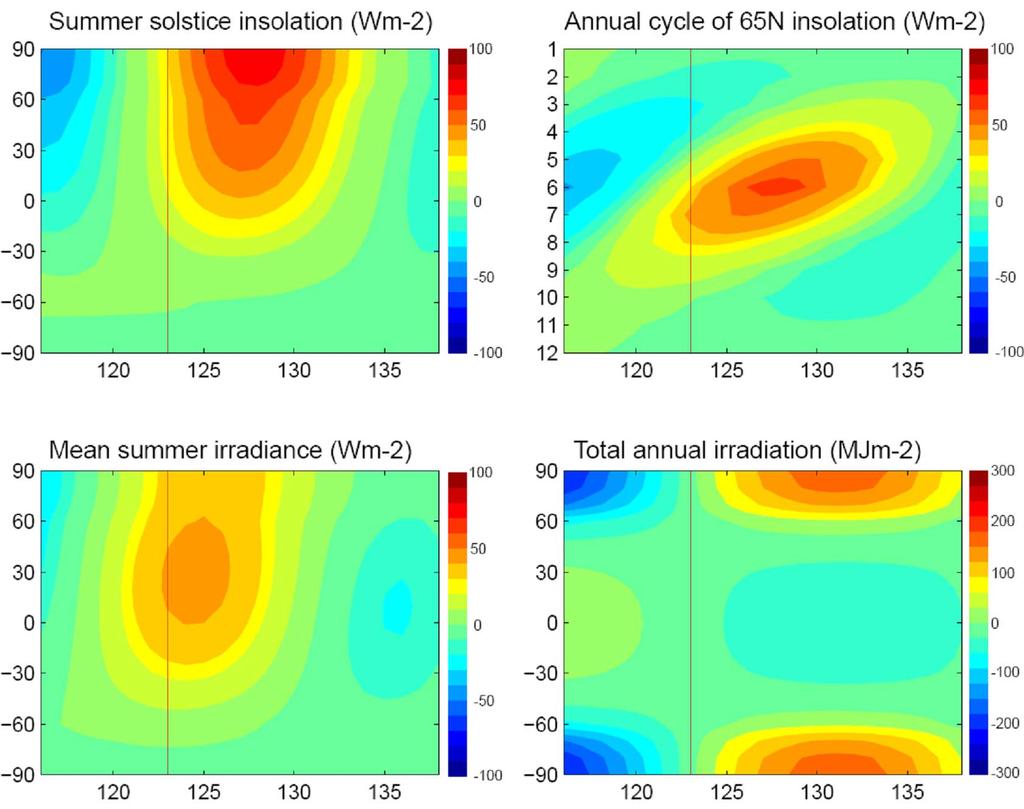
111

112 800 CH 4 (ppb) CO 2 (ppm) Age (ka)

113 Inception TII 0 δ 18 O ( ) MIS RSL (m) 4.0 MIS 5d δd ( ) Early maximum Age (ka) CH 4 (ppb)

114

115

116

117

118

119

120

121

122

123

124

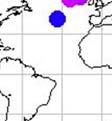
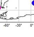
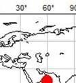
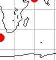
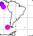
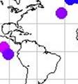
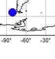
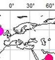
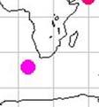
125 5e 11c 7e 13a

126

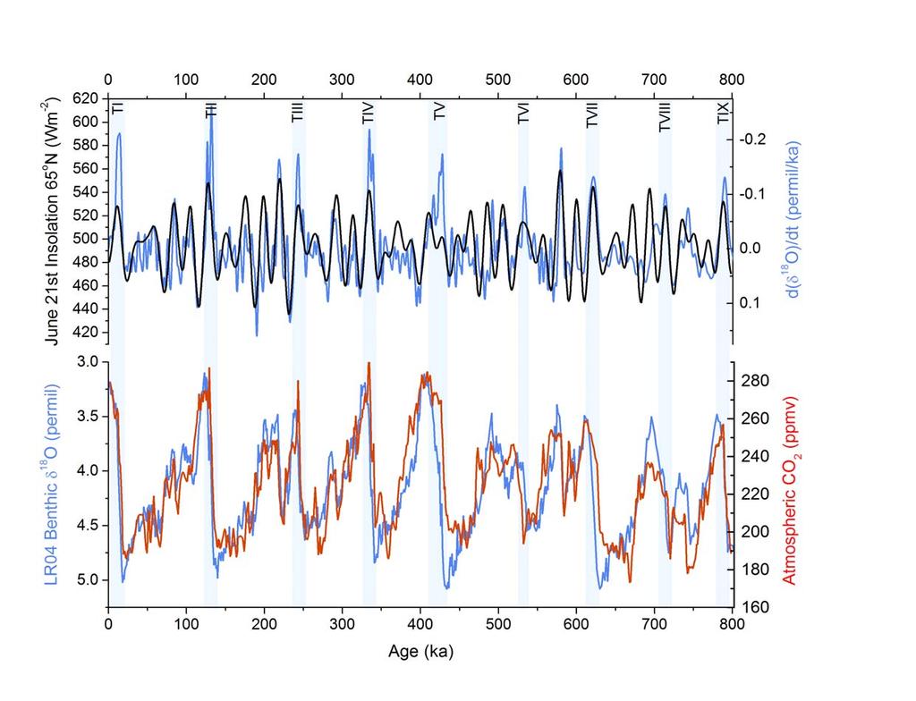
127