Land Degradation Monitoring Tool

Transcription

1 Land Degradation Monitoring Tool -Guidance Document - Land Degradation Monitoring Tool; Version 1 September 27, 2017 Part of the project Enabling the use of global data sources to assess and monitor land degradation at multiple scales Prepared by: Mariano Gonzalez-Roglich, Conservation International Yengoh Genesis, Lund University Monica Noon, Conservation International Lennart Olsson, Lund University Mariano Gonzalez-Roglich, Conservation International Tristan Schnader, Conservation International Anna Tengberg, Lund University Alex Zvoleff, Conservation International

2 Table of Contents: 1) Before installing the toolbox 3 2) Installing the toolbox 3 3) Settings 6 4) Download data 8 5) Calculate Indicators 10 a) Productivity 11 Summary 11 Productivity Trajectory 12 Calculating Trajectory 12 Productivity Performance 14 Calculating Performance 15 Productivity State 15 Calculating State 16 Productivity Area of interest 16 Submit task 17 b) Land Cover 17 Summary 17 Calculating Land cover changes 18 Land cover Area of interest 20 c) Soil Carbon 20 6) View Google Earth Engine Tasks 21 7) Visualizing results in QGIS 21 Visualizing results from Productivity Trajectory 22 Visualizing results from Productivity Performance 23 Visualizing results from Productivity State 25 Visualizing results from Land Cover Change 27 8) Plot Data 29 9) Reporting Tool 31 10) Info 32 11) References 33 2 of 39

3 1) Before installing the toolbox Before installing the toolbox, QGIS version 2.18 or higher (64 bit) needs to be installed in the computer. QGIS can be downloaded from: Once the installer is downloaded from the website, it needs to be run (double click on it). Select the options using the Default settings. 2) Installing the toolbox There are two methods to install the toolbox. The preferred one is through QGIS. For that, launch QGIS (Go to your Start > Programs menu to launch QGIS), then go to Plugins In the menu bar at the top of the program and select Manage and install plugins. 3 of 39

4 Then search for a plugin called Land degradation monitoring tool and select Install plugin at the bottom right of the screen. If your plugin has been installed properly, there will be a toolbox in the top left of your browser The second installation method is manual. For that, first make sure QGIS is closed. Then you ll need to download the toolbox file from: The file needs to be unzipped, and the LDMP folder needs to be copied into your QGIS Plugin Folder: D:\Documents and Settings\USER\.qgis2\python\plugins USER: will be replaced by the user name of the windows session. In this example mnoon. 4 of 39

5 Now open QGIS, Select Plugins > Manage and install plugins, place a check next to the Land Degradation Monitoring Tool. The toolbox bar should appear in the QGIS menu. 5 of 39

6 Scrolling over each of the icons will display a text pop up with the description of each icon category on the toolbar. Settings Raw download Calculate indicators View GEE Tasks Plot data Reporting tool About 3) Settings This is the registration page to use the plugin. Users must register their address to obtain a free account. Select the wrench to go to Settings. Here you can register as a new user or Login with your credentials. 6 of 39

7 To Register, select the Register button and enter your , Name, Organization and Country of residence and select Register user A unique password will be sent to your . Please check your Junk folder if you cannot find it within your inbox. The will come from ldmp-api@resilienceatlas.org. 7 of 39

8 Enter your credentials and Login. 4) Download data To work offline, you will be able to select an area of interest or upload a shapefile to download your relevant datasets and work in areas with limited or no internet access. This feature is currently unavailable. 8 of 39

9 The table below describes all the data available through the toolbox. It specifies data sources, resolutions, coverage and the different indicators for which each data set is used. 3 m -3 * (0-7 cm) 3 m -3 9 of 39

10 5) Calculate Indicators Sustainable Development Goal 15.3 intends to combat desertification, restore degraded land and soil, including land affected by desertification, drought and floods, and strive to achieve a land degradation-neutral world by In order to address this, we are measuring primary productivity, land cover and soil carbon to assess the annual change in degraded or desertified 10 of 39

11 arable land (% of ha). The Calculate indicators button brings up a page that allows calculating datasets associated with the three SDG Target 15.3 sub indicators. For productivity and land cover, the toolbox implements the Tier 1 recommendations of the Good Practice Guidance lead by CSIRO. For productivity, users can calculate trajectory, performance, and state. For Land Cover, users can calculate land cover change relative to a baseline period, and enter a transition matrix indicating which transitions indicate degradation, stability, or improvement. Select which Indicator you would like to calculate Productivity: measures the trajectory, performance and state of primary productivity Land cover: calculates land cover change relative to a baseline period, enter a transition matrix indicating which transitions indicate degradation, stability or improvement. Soil carbon: under review following the Good Practice Guidance (CSIRO, ). a) Productivity Summary Productivity measures the trajectory, performance and state of primary productivity using either 8km GIMMS3g.v1 AVHRR or 250m MODIS datasets. The user can select one or multiple indicators to calculate, the NDVI dataset, name the tasks and enter in explanatory notes for their intended reporting area. NOTE: The valid date range is set by the NDVI dataset selected within the first tab: AVHRR dates compare and MODIS of 39

12 Productivity Trajectory 1) Trajectory is related to the rate of change of productivity over time. a) Users can select NDVI trends, Rain Use Efficiency (RUE), Pixel RESTREND or Water Use Efficiency (WUE) to determine the trends in productivity over the time period selected. b) The starting year and end year will determine de period on which to perform the analysis. c) The initial trend is indicated by the slope of a linear regression fitted across annual productivity measurements over the entire period as assessed using the Mann-Kendall Z score where degradation occurs where z= (CSIRO, 2017). d) Degradation in each reporting period should be assessed by appending the recent annual NPP values (measured in the toolbox as annual integral of NDVI) to the baseline data and calculating the trend and significance over the entire data series and the most recent 8 years of data (CSIRO, 2017). e) Climate datasets need to be selected to perform climate corrections using RESTREND, Rain Use Efficiency or Water Use Efficiency (refer to table 1 for full list of climate variables available in the toolbox). Calculating Trajectory 1) Check next to Trajectory 2) Select NDVI dataset to use 12 of 39

13 3. Assign a name to the task. Use descriptive names including study area, periods analyzed and datasets used, to be able to refer to them later. 4. In the tab Trajectory, select the method to be used to compute the productivity trajectory analysis. The options are: NDVI trend: This dataset shows the trend in annually integrated NDVI time series ( ) using MODIS (250m) dataset (MOD13Q1) or AVHRR (8km; GIMMS3g.v1). The normalized difference vegetation index (NDVI) is the ratio of the difference between near-infrared band (NIR) and the red band (RED) and the sum of these two bands (Rouse et al., 1974; Deering 1978) and reviewed in Tucker (1979). Rain use efficiency (RUE): is defined as the ratio between net primary production (NPP), or aboveground NPP (ANPP), and rainfall. It has been increasingly used to analyze the variability of vegetation production in arid and semi-arid biomes, where rainfall is a major limiting factor for plant growth Pixel RESTREND: The pointwise residual trend approach (P-RESTREND), attempts to adjust the NDVI signals from the effect of particular climatic drivers, such as rainfall or soil moisture, using a pixel-by-pixel linear regression on the NDVI time series and the climate signal, in this case precipitation from GCPC data at 250m resolution. The linear model and the climatic data is used then to predict NDVI, and to compute the residuals between the observed and climate-predicted NDVI annual integrals. The NDVI residual trend is finally plotted to spatially represent overall trends in primary productivity independent of climate. 13 of 39

14 Water use efficiency (WUE): refers to the ratio of water used in plant metabolism to water lost by the plant through transpiration. Productivity Performance Performance is a comparison of how productivity in an area compares to productivity in similar areas at the same point in time. Select the period of analysis. This determines the initial degradation state and serves as a comparison to assess change in degradation for each reporting period. The initial productivity performance is assessed in relation to the 90 th percentile of annual productivity values calculated over the baseline period amongst pixels in the same land unit. The toolbox defines land units as regions with the same combination of Global Agroecological Zones and land cover (300m from ESA CCI). Pixels with an NPP performance in the lowest 50% of the distribution for that particular unit may indicate degradation in this metric (CSIRO, 2017). 14 of 39

15 Calculating Performance 1. Select the baseline period of comparison. This determines the initial degradation state and serves as a comparison to assess change in degradation for each reporting period. 2. The initial productivity performance is assessed in relation to the 90 th percentile of annual productivity values calculated over the baseline period amongst pixels in the same land unit. Pixels with an NPP performance in the lowest 50% of the historical range may indicate degradation in this metric (CSIRO, 2017). 3. Contemporary Productivity Performance for each reporting period should be calculated from an average of the years between the previous (or baseline) assessment up to the current year (CSIRO, 2017). Productivity State State is a comparison of how current productivity in an area compares to past productivity in that area. o The user selects the baseline period and comparison period to determine the state for both existing and emerging degradation. o The baseline period classifies annual productivity measurements to determine initial degradation. Pixels in the lowest 50% of classes may indicate degradation (CSIRO, 2017). o Productivity State assessments for each reporting period should compare the average of the annual productivity measurements over the reporting period (up to 4 years of new data) to the productivity classes calculated from the baseline period. NPP State classifications that have changed by two or more classes between the baseline and reporting period indicate significant productivity State change (CSIRO, 2017). 15 of 39

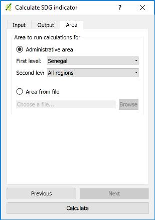
16 Calculating State 1. The user selects the baseline period and comparison period to determine the state for both existing and emerging degradation. 2. The baseline period classifies annual productivity measurements to determine initial degradation. Pixels in the lowest 50% of classes may indicate degradation (CSIRO, 2017). 3. productivity State assessments for each reporting period should compare the average of the annual productivity measurements over the reporting period (up to 4 years of new data) to the productivity classes calculated from the baseline period. NPP State classifications that have changed by two or more classes between the baseline and reporting period indicate significant productivity State change (CSIRO, 2017). Productivity Area of interest The final step before submitting the task to Google Earth Engine, is to define the study area on which to perform the analysis. The toolbox allows this task to be completed in one of two ways: 1. The user selects first (i.e. country) and second (i.e. province or state) administrative boundary from a drop down menu. 2. The user can upload a shapefile with an area of interest. NOTE: This boundary should have only one polygon, i.e. when uploading a country with outlying islands, there will be multiple geometries drawn separately. By merging the polygons, the analysis will be run on the entire study area as opposed to a single polygon. 16 of 39

17 Submit task When all the parameters have been defined, click Calculate, and the task will be submitted to Google Earth Engine for computing. When the task is completed (processing time will vary depending on server usage, but for most countries it takes only a few minutes most of the time), you ll receive an notifying the successful completion. b) Land Cover Summary Changes in land cover is one of the indicators used to track potential land degradation which need to be reported to the UNCCD and to track progress towards SDG While some land cover transitions indicate, in most cases, processes of land degradation, the interpretation of those transitions are for the most part context specific. For that reason, this indicator requires the input of the user to identify which changes in land cover will be considered as degradation, improvement or no change in terms of degradation. The toolbox allows users to calculate land cover change relative to a baseline period, enter a transition matrix indicating which transitions indicate degradation, stability or improvement. 17 of 39

18 Calculating Land cover changes 1) Click on the Calculate Indicators button from the toolbox bar, then select Land cover. 2) Set up tab: Allows the user to select the starting year and ending year a) The baseline should be considered over an extended period over a single date (e.g. 1/1/ /31/2015). b) User selects target year. c) Metadata: User enters unique task name and notes for the analyses. 3) Transition matrix tab a) User selects the transition matrix value of land cover transitions for each transition between the 6 IPCC land cover classes. For example: i) The default for cropland to cropland is 0 because the land cover stays the same and is therefore stable. 18 of 39

19 ii) The default for forest to cropland is -1 because forest is likely cut to clear way for agriculture and would be considered deforestation. iii) The transition can be defined as stable in terms of land degradation, or indicative of degradation (-1) or improvement (1). b) Users can keep the default values or create unique transition values of their own. By default, and following the CSIRO best practices guidance document, the major land cover change processes that are classified as degradation are: 1) Deforestation (forest to cropland or settlements) 2) Urban expansion (grassland, cropland wetlands or otherland to settlements) 3) Vegetation loss (forest to grassland, otherland or grassland, cropland to other land) 4) Inundation (forest, grassland, cropland to wetlands) 5) Wetland drainage (wetlands to cropland or grassland) 6) Withdrawal of agriculture (croplands to grassland) 7) Woody encroachment (wetlands to forest) The major land cover change processes that are not considered degradation are: 1) Stable (land cover class remains the same over time period) 2) Afforestation (grassland, cropland to forest; settlements to forest) 3) Agricultural expansion (grassland to cropland; settlements or otherland to cropland) 4) Vegetation establishment (settlements or otherland to settlements) 5) Wetland establishment (settlements or otherland to wetlands) 19 of 39

20 6) Withdrawal of settlements (settlements to otherland) It is important to remember that those are suggested interpretations, and should be evaluated and adjusted considering the local conditions of the regions in for which the analysis will be performed. Land cover Area of interest The final step before submitting the task to Google Earth Engine, is to define the study area on which to perform the analysis. The toolbox allows this task to be completed in one of two ways: 1. The user selects first (i.e. country) and second (i.e. province or state) administrative boundary from a drop-down menu. 2. The user can upload a shapefile with an area of interest. c) Soil Carbon SOC indicator calculation coming soon! 20 of 39

21 6) View Google Earth Engine Tasks Users can view their current and previous tasks here. The unique task name provided by the user, which analysis is running (job), the start time and end time of when the task was started and completed and whether or not the task was successful. The Details page outlines the reason a task may have failed. To download the results to the computer click on Download results and a window will pop up, to select the location in which to store the raster files and click on Select Folder. 7) Visualizing results in QGIS Once the results are downloaded (this could take a few minutes depending on the size of the area analyzed and the internet connection speed), they will automatically load in QGIS. The results from each analysis will be loaded with its corresponding symbology. 21 of 39

22 Visualizing results from Productivity Trajectory Parameters used: Visualizing in QGIS: The first layer is the Productivity trajectory trend layer: 22 of 39

23 The second layer added is a classified version of the layer above. The classes are: Visualizing results from Productivity Performance Parameters used: 23 of 39

24 Visualizing in QGIS: The productivity performance indicator layer output has 5 classes: 24 of 39

25 Visualizing results from Productivity State Parameters used: Visualizing in QGIS: The productivity state initial degradation indicator layer output has 5 classes: 25 of 39

26 The productivity state emerging degradation indicator layer output has 6 classes: 26 of 39

27 Visualizing results from Land Cover Change Parameters used: Visualizing in QGIS: The land cover change analysis produces four raster outputs. The land cover baseline and target layers have 6 classes: Baseline land cover: 27 of 39

28 Target land cover: The land cover change layer has 36 classes, where beige indicate regions in which land cover did not change between the baseline and target periods. 28 of 39

29 The land cover degradation layer has 3 classes: 8) Plot Data 29 of 39

30 The toolbox also supports plotting time series showing how a particular indicator has changed over time. To use this feature, click on the Plot data button from the toolbox bar. Then se;ect a dataset, indicator, and area to plot: When all the parameters have been defined, click Calculate, and the task will be submitted to Google Earth Engine for computing. When the task is completed (processing time will vary depending on server usage, but for most countries it takes only a few minutes most of the time), you ll receive an notifying you of the successful completion of the task. Use the Download tool described above to download and plot the results: 30 of 39

31 9) Reporting Tool Using the analyses from the former set of steps (under the Calculate indicators tab), there is a set of outputs currently displayed within the QGIS window. Select the Reporting Tool in the LDMT. The Land degradation reporting window will appear. Click on SDG Target Indicator to aggregate the analyses. The output layer can be selected using the existing layers within the map: Productivity trajectory trend (significance), productivity performance (degradation), Productivity (emerging) and Land Cover (degradation). Then select where the output will be saved and the area of interest for the final degradation map. This analysis is run locally in QGIS and will automatically appear in your map window. 31 of 39

32 10) Info 32 of 39

33 11) Interpreting results The three metrics (trend, state and performance) are aggregated to determine if land is degraded in areas where productivity may be increasing but remains low relative to other areas with similar land cover characteristics and climatic conditions. Areas with a statistically significant negative trend over time indicate a decline in productivity. When both performance and state show potential degradation, the assessment indicates negative productivity as well. The LDMT allows users to select the trajectory indicatory method to detect productivity. Selecting NDVI Trends for the baseline period will yield the following two outputs: (left) Productivity trajectory trend (significance) and (right) Productivity trajectory trend (slope of NDVI) for East Africa and Senegal. 33 of 39

34 Performance is a measurement of local productivity relative to other similar vegetation types in similar land cover types and bioclimatic regions (areas of similar topographic, edaphic and climatic conditions). The initial baseline value for land productivity, from which future changes are compared, is in the above performance output. 34 of 39

35 State compares the current productivity level in a given area to historical observations of productivity in that same area. Assessments are completed for a given location over time, as an indicator of the current state of vegetation productivity. These three-metrics help determine if land is degraded in areas where productivity may be increasing but remains low relative to other areas with similar land cover characteristics and climatic conditions. In this assessment, changes in productivity are considered negative when there is a statistically significant negative trend over time, or when both the Performance and State assessments indicate potential degradation, including in areas where the trend is not significantly negative (CSIRO 2017). In order to interpret the likelihood of results indicating false positives or false negatives, a lookup table is used to identify support class combinations of metrics in each pixel (CSIRO 2017). Classes 1-5 indicate degradation. 35 of 39

36 The assessment and evaluation of land cover changes are derived from the European Space Agency Climate Change Initiative Land Cover (ESA-CCI-LC) 300m product. These are aggregated into the IPCC major land cover classes: Forest land, grassland, cropland, wetlands, settlements and other land. Degradation can be identified through land cover as: 1) a decline in the productive capacity of the land, through loss of biomass or a reduction in vegetation cover and soil nutrients, 2) a reduction in the land s capacity to provide resources for human livelihoods, 3) a loss of biodiversity or ecosystem complexity, and 4) an increased vulnerability of population or habitats to destruction at the national scale (CSIRO 2017). 36 of 39

37 Land cover transitions are designated by the user via the transition matrix. This example, using the default in the LDMT, the beige color indicate areas where no change has occurred. The remaining pixels highlighted demonstrate the transition from the baseline ( ) to the target year (2015). A closer look (below) shows transitions in central Tanzania of conversion from croplands (red) or forest land (green) to other land cover classes. The transition matrix has both default values and the option to select the transition values within the context of the specified area of interest. The matrix allows users to define 30 possible transitions. The unlikely transitions are highlighted above (left) in red text with major land cover 37 of 39

38 processed (flows) noted. The boxes are color coded as improvement (green), stable (blue) or degradation (red) using land cover/land use change for the 6 IPCC classes (CSIRO 2017). The table (above right) demonstrates how the description of major land cover change processes are identified as flows. Note that some transitions between classes will not yield logical results. Calculating the final indicator is done using the pie chart symbol in the LDMT. The output layer can be selected using the existing layers within the map: Productivity trajectory trend (significance), productivity performance (degradation), Productivity (emerging) and Land Cover (degradation). These are aggregated to highlight degradation given the inputs and parameters from former analyses. 38 of 39

39 The final output show degradation in red and improvement in green excluding the urban and water values from the output. Given the analyses prior to the we can conclude that the areas in red have been degraded using as a baseline for NDVI Trend (trajectory), for performance, for emerging baseline with 2015 as the target year of comparison for degradation. Land cover highlighted the transition from the baseline ( ) to the target year (2015) using the standard default transitions to identify degradation. Together these were aggredated to forumulate the final degradation output above. This notes degradation within central Uganda. 12) References CSIRO, Good Practice Guidance. SDG Indicator : Proportion of land that is degraded over total land area. September of 39