Mesoscale atmospheric modeling of the San Francisco Bay Area using the Weather Research & Forecasting model (WRF)

Transcription

1 Mesoscale atmospheric modeling of the San Francisco Bay Area using the Weather Research & Forecasting model (WRF) Jian Wilson Dong August 1, 29 Abstract A fully compressible and non-hydrostatic Numerical Weather Prediction (NWP) model called the Weather Research & Forecasting (WRF) model is used to model atmospheric ow over the San Francisco Bay Area. Simulations are done in WRF using ne resolutions grids and twoway nesting. Atmospheric ow over SF Bay Area must take into account the inuence of underlying topography and land cover, including hills, buildings, etc. Due to the complex terrain and heterogeneous land cover, high-resolution simulations are needed to accurately describe the ow. Simulations are performed at 9km and 3km horizontal resolutions as well as 6km and a two way nested domain of 2km for two dierent days. Typical NWP models are run at 12km resolution. The simulations results are compared to radiosonde observations at the Oakland Airport on various dates to provide insights to how well WRF performs at ner resolutions than what is typically used for weather forecasting. 1

2 Contents 1 Introduction 3 2 Background & Theory Continuity Equation Navier-Stokes Equations Energy Equation - First Law of Thermodynamics Scalar Transport Equation Runge-Kutta Time Integration Scheme Methodology & Approach WRF Pre-processing System (WPS) WRF Post-Processing Visualization Approach Results Radiosonde and Simulation Comparisons NCL Visualizations Discussion Simulation & Radiosonde Comparison Relative Humidity and Satellite Image Comparison General Remarks Conclusion 25 7 Acknowledgements 26 2

3 1 Introduction The San Francisco Bay Area can display a variety of meteorological conditions simultaneously. The hills, winds, fog, ocean and bay strongly aect local weather, resulting in "microclimates" where weather can be very dierent depending on the exact location. For example, San Francisco and San Jose are separated by a distance of less than 5 miles but can experience temperature dierences of greater than 2 degrees Fahrenheit. This makes microweather prediction very dicult using the typical 12km grid resolutions used in operational weather forecasting. Therefore, there exists a need for ner grid resolution to better simulate the weather in the Bay Area which is strongly inuenced by complex topography and proximity to large bodies of water. Increasingly sophisticated computational uid dynamics software and computational powers have rendered Numerical Weather Prediction (NWP) systems progressively more indispensable in the simulations of weather phenomena. Mesoscale modeling is capable of forecasting weather in the range of several kilometers to several hundred kilometers per grid. Many weather occurrences manifest at the mesoscale level: tornadoes, turbulence, and other phenomena forced by coastlines or topography. Mesoscale modeling can also produce superior forecasts in coastal and mountainous terrains where higher resolutions are desired. The Weather Research & Forecasting (WRF) model is a mesoscale NWP system capable of modeling of suciently high grid resolutions, from several meters to several thousand meters. Developed primarily by National Center for Atmospheric Research (NCAR) and other research facilities, WRF is used for both operational weather forecasting and for research advancements in computational uid dynamics and atmospheric sciences. In the words of the creators of WRF[1], The WRF model is a fully compressible and non-hydrostatic model (with a runtime hydrostatic option). Its vertical coordinate is a terrain-following hydrostatic pressure coordinate. The grid staggering is the Arakawa C-grid. The model uses the Runge-Kutta 2nd and 3rd order time integration schemes, and 2nd to 6th order advection schemes in both horizontal and vertical. It uses a time-split small step for acoustic and gravity-wave modes. The dynamics conserves scalar variables. The model also supports one-way, two-way and moving nest options. It runs on single-processor, shared- and distributed-memory computers. WRF is used to model atmospheric ow over the general San Francisco Bay Area using ne resolutions: 9km and 3km individually, and 6km with a twoway nesting of 2km. All are compared to radiosonde data from the Oakland Airport to test the accuracy of the simulations at various resolutions. WRF executes the equations of motions and many physical parameterizations on a grid system. Hence, the more complex the terrains over which a simulation runs, the more dicult it is to accurately represent the topography and the resulting ow features. Altering the horizontal grid resolutions allows for the assessment of whether or not ner grid resolutions help achieve better comparison with actual observations. 3

4 2 Background & Theory At the core of all computational uid dynamics simulation software are the fundamental laws of uid mechanics and thermodynamics. They consist of mainly of three sets of equations: Navier-Stokes equations for the conservation of momentum, the continuity equation for the conservation of mass, and the thermal energy equation for the conservation of energy. These primitive equations describe the way which uid ows and energy is transferred in the atmosphere. 2.1 Continuity Equation The continuity equation is a partial dierential equation that describes the transport of a conserved quantity: mass. In plain words, the continuity equation states that the rate at which mass enters any innitesimal control volume must equal the rate at which mass leaves the control volume plus any change in the density (accumulation) of the uid with respect to time. Mathematically, the continuity equation in Cartesian coordinates is as follows: ρ + (ρv) = (1) t where ρ is the density of the uid and V is the velocity vector, and is the gradient operator. Upon expansion, equation 1 is expressed as ρ t + (ρv) x + (ρu) + (ρw) = y z This form of conservation of mass for a innitesimal control volume requires no assumptions as long as density and the velocity vector are continuum functions. The equation is valid for compressible or incompressible, steady or unsteady, and viscous or friction-less ow as long as there is no source or sink singularities within the element. 2.2 Navier-Stokes Equations All NWP models rely on the use of a version of the momentum equations. These equations of motion describe the balance among the friction encountered by a uid, the pressure and external forces acting on the uid and the inertia of the uid. This can be compactly written as: ρ DV [ ] dv Dt = ρ dt + V V = P + τ ij + f (2) where DV Dt is the substantial (total) derivative, P is the pressure function, τ ij is the stress tensor, and f is the body force exerted on the uid, namely, gravity and Coriolis. In the explanation of the NS equations, the Coriolis force is excluded. Equation 2 is the full-blown momentum equation and is so deceivingly brief and concise that one may not grasp its innate complexity. Expanding the vector equation yields three component equations (x, y, z) each with nine terms. 4

5 ( u ρ t + u u x + v u y + w u ) = P z x + τ xx x + τ yx y + τ zx z + ρg x ( v ρ t + u v x + v v y + w v ) = P z y + τ xy x + τ yy y + τ zy z + ρg y ( w ρ t + u w x + v w y + w w ) = P z z + τ xz x + τ yz y + τ zz z + ρg z To simplify, the application of the constitutive laws and the assumption of Newtonian uid is employed; that is, the viscous terms are proportional to the strain rate and the viscosity of the uid. This yields ρ ( u t + u u x + v u y + w u ) z = P x + µ ( 2 u x u y u z 2 ) + ρg x ( v ρ t + u v x + v v y + w v ) = P ( 2 ) z y + µ v x v y v z 2 + ρg y ( w ρ t + u w x + v w y + w w ) = P ( 2 ) z z + µ w x w y w z 2 + ρg z These are known as the set of Navier-Stokes equations. They are a set of second-order, non-linear partial dierential equations with no known general solution. In this form they can be written compactly as [ ] V ρ t + V V = P + µ 2 V + f (3) The Navier-Stokes equations state that density acceleration = pressure gradient force per unit volume + viscous force per unit volume + gravity force per unit volume. There are many variations of the Navier-Stokes equations, such as the Reynolds-averaged Navier Stokes equations for turbulent ow, which have a similar form to Equation 3 except that the molecular viscosity is replaced by a turbulent eddy viscosity to account for the eects of turbulent mixing. However elegant they look, these sets of equal are notoriously dicult to solve analytically. There are only a handful of exact solutions for simple uid ow problems; the majority of Navier Stokes problems are solved numerically using computational uid dynamics, such as WRF. 5

6 2.3 Energy Equation - First Law of Thermodynamics The energy equation is given by ρ Dû + P ( V) = (k T ) + Φ (4) Dt where û is the specic internal energy, T is the temperature in Kelvin, k is the thermal conductivity coecient, Φ is the viscous-dissipation function, [ ( u ) 2 ( ) 2 ( ) ] 2 v w Φ = 2µ x y z [ ( v µ x + u ) 2 ( w + y y + v ) 2 ( u + z z + w ) ] 2 (5) x Equation 4 is valid for any Newtonian uid under general conditions of unsteady, viscous, compressible and heat conducting ow. Often, the following assumptions are made: Dû c v dt and c v, ρ, k, µ = constant. Thus equation 4 is rewritten as ρc v DT Dt = ρc v ( T t + u T x + v T y + w T ) = k 2 T + Φ (6) z Notice that for a static uid, the viscous-dissipative function drops out, and what is left is the heat-conduction equation: T ρc v t = k 2 T (7) The heat conduction equation is relevant for a stable atmosphere, in which there is no convective heat transfer. It can be used to explain heat ow in the absence of atmospheric mixing (for example, the presence of a temperature inversion layer). 2.4 Scalar Transport Equation Although the equations of mass, momentum and energy conservation are required in describing atmospheric uid motion, many other atmospheric physics equations are needed to describe the transport mechanism of certain quantities or substances within a moving uid. The uid motion can be described as a vector eld of time and space, while the scalar function describes the amount of stu that is conserved within the contained uid. This can be explained by a general scalar transport equation: (ρφ) + (ρφv) = (Γ φ) + S φ } t {{}}{{}}{{}}{{} convection term diffusion term source term transient term (8) 6

7 where φ is the scalar quantity of a substance (for example, humidity or moisture), V is the known velocity eld of the uid, Γ is the diusion coecient and S φ is the source term. More specically, transient term accounts for any accumulation or change in density of the scalar φ in a given innitesimal control volume. convection term accounts for the transport of the scalar φ due to the presence of a velocity eld. diusive term accounts for the transport of the scalar φ due to gradients. source/sink term accounts for any local production or destruction of the scalar φ. The scalar transport equation can be used to describe the distribution in time and space of many conserved scalar quantities. In atmospheric uid ow, they include precipitation of water from clouds in addition to other cloud variables, like ice, snow, hail, graupel, cloud water and humidity. 2.5 Runge-Kutta Time Integration Scheme The third order of Runge-Kutta numerical method is used to advance the time integration of WRF. It integrates dierential equations using a predictorcorrector formulation. If we dene our prognostic variables as Φ, and our model equation as Φ t = R(Φ), we would need to form three steps to advance one solution, from Φ(t) to Φ(t + t). 3 Methodology & Approach Φ = Φ t + t 3 R(Φt ) (9) Φ = Φ t + t 2 R(Φ ) (1) Φ t+ t = Φ t + tr(φ ) (11) A Windows machine is used to connect, via Cygwin, to a Linux server which does the actual conguration, compilation and computation of WRF and its pre-processor. 3.1 WRF Pre-processing System (WPS) Before running WPS or WRF, a number of steps has to be completed. These include getting all the necessary libraries needed for WRF. They include netcdf, GRIB2 libraries, and a post-processing visualizer such as NCL. WPS was con- gured and compiled using a serial gfortran compiler. 7

8 Figure 1: WPS Flowchart[2] WPS consists of a set of three programs that collects and prepares the input data into WRF. The three programs are geogrid.exe, ungrib.exe and metgrid.exe. Geogrid's purpose is to dene the simulation domains and to extract the various static terrestrial data sets onto the model grids. These include computing the latitude, longitude, and map scale factors. It will also determine the necessary terrain properties such as the soil categories, the land use category, the terrain height, the mean soil temperature, the albedo, and so on. Geogrid options can be edited under the geogrid section of namelist.wps. Ungrib's purpose is to read in GRIB les and degrib the data so that it can be written in a simple format, called the intermediate format. The GRIB les are comprised of time-varying meteorological data which are usually from regional or global data models. Simulation data was attained from the NOAA's North America Mesoscale (NAM) model database to provide initial and lateral boundary conditions at 12km horizontal resolution. Ungrib options can be edited under the ungrib section of namelist.wps Metgrid maps the meteorological data extracted by the ungrib program onto the land domains extracted by the geogrid program. The output of the metgrid program is used as the input to the WRF real program. Metgrid options can be edited under the metgrid section of namelist.wps. Ungrib, geogrid, and metgrid all refer to the same text le, namelist.wps, to attain the simulation dates, part of the simulation options and the geographical domain over which simulation is performed. 3.2 WRF WRF consists of two programs: real.exe and wrf.exe. Real.exe is the WRF initialization program that vertically interpolates meteorological elds to WRF eta levels; wrf.exe is the numerical integration program. Most options and physics schemes can be edited in a le called namelist.input (which diers from 8

9 Figure 2: WRF Flowchart[2] namelist.wps in WPS) in the directory in which real.exe and wrf.exe are located. Namelist.input must match its WPS counterpart namelist.wps or else the simulation might output an error. Namelist.input includes many more options that can be turned on or o. A partial list of namelist variables to edit are: start_*, end_* : the start time and end time of the simulation interval_seconds: the time interval between input data which provides the lateral boundary conditions time_step: model time step of integration e_ws, e_sn, e_vert: the domain dimensions in west-east, south-north and in the vertical coordinate dx, dy: the grid resolution in meters max_dom: the number of domains in the simulation ref_lat, ref_lon: latitude and longitude of coarse domain's center-point The output from real.exe is fed into wrf.exe which then outputs the simulation results. These results can be visualized using many dierent post-processing softwares and visualizers. 3.3 Post-Processing Visualization To visualize the output from wrf.exe, the primary software used is the NCAR Command Language (NCL). NCL is an interpreted language designed by the 9

10 National Center for Atmospheric Research specically for the processing and visualization of scientic data. The graphics outputs by NCL are highly customized to the user's need. The graphics produced by NCL is publication quality. Despite being an interpreted language, NCL has similarities to programming languages as it includes operators, loops, variables, etc. It is robust and powerful, hence why it is used for visualization of the model data. NCL is capable of writing ASCII les. NCL scripts are written to extract data from WRF simulations. The ASCII les outputted by NCL are read in by matlab and subsequently plotted. See the following subsection for more details. 3.4 Approach WRF simulation is performed for two days: June 21, 29 and July 11, 29. For all cases, the following namelist.input options is chosen: Lambert conformal mapping is used. Geographical domain centered at latitude, longitude. Simulation is performed for 18 hours. Time interval between incoming NAM meteorological data is 6 hours. The incoming data is used to initialize the conditions and provide lateral boundary conditions. Data for initialization is input at Z, data for lateral boundary conditions are input at 6Z, 12Z and 18Z and interpolated in between. Time interval between WRF output data is 3 hours. 3 vertical levels. Boundary-layer physics is called at every time step (option ). Microphysics (mp_physics) scheme is set to WRF single-moment 3-class scheme (option 3). Longwave Radiation (ra_lw_physics) is set to the Rapid Radiative Transfer Model scheme (option 1). Shortwave Radiation (ra_sw_physics) is set to Duhia scheme (option 1). Surface Layer physics (sf_sfclay_physics) is set to Monin-Obukhov scheme (option 1). Land Surface physics (sf_surface_physics) is set to the Noah Land Surface Model (option 2). The Planetary Boundary Layer physics (bl_pbl_physics) uses the Yonsei University scheme (option 1). 1

11 Figure 3: Geographical Domains: 9km, 6km & its nested 2km, 3km Cumulus Parameterization (cu_physics) is set to the Kain-Fritsch scheme (option 1). Diusion Option is set to use the simple diusion option, in which gradients are taken along coordinate surfaces (option 1). Damping (damp_opt) is set to none (option ). The June 21, 29 case consists of three runs: one single-domain run at 9km, another at 3km over the greater San Francisco Bay Area, and then a 6km and 2km two-way nested domain over the San Francisco Bay Area. The July 11, 29 simulation run consists of only a 6km and its 2km two way nested run. The geographical domains for all three resolutions for all the runs are shown in gure 3: For all three runs, the simulation start date is at , Z and the simulation end date is at , 18Z. In the 9km and 3km simulation runs, WRF is set up with the following namelist options (in addition to those specied before): Grid resolution of 9km or 3km Grid number of 51 in the x and y horizontal grids Integration time step of 27 seconds For the 6km and its 2km nested domain, a two-way nested run is utilized. A two-way nested run allows for simultaneous communication between multiple domains of dierent grid resolutions. The larger domain can provide boundary values for the smaller nest domain, and the nest can feed its ner calculation back to the larger domain. Nested runs (both the June 21 and July 11 runs) use the following options: Integration time step of 16 seconds for the parent domain, a third of that (5.333 seconds) for the nested domain. 11

12 6 kilometers grid resolution for the parent domain, a third of that for the nested domain. Grid numbers of 48 for the parent domain and 49 for the nested domain. The goal is to compare radiosonde data from the Oakland International Airport to the simulation data produced by the WRF. Necessary data from all the WRF output les are extracted using NCL. Scripts are written in NCL to extract data of variables of interest at the grid point that contains the location of the Oakland International Airport. The variables is plotted with the same variables observed by the radiosonde to assess the accuracy of the simulations. These variables include Pressure Potential temperature Relative humidity Wind speed Direction All ve variables are plotted against height to display the degree to which simulation reects observation. WRF simulations at the initial time Z and at 12Z is compared to Oakland Airport radiosonde data at Z and 12Z for both days. The Pacic Division Time is 7 hours behind the Universal Time Coordinates (Z). Therefore, in Pacic Division Time, the simulations from Z to 18Z is actually from 17PDT (5pm) to 11PDT (11am). Additionally, visualizations done in NCL are provided. The focus is on the prediction of fog, therefore the contour plots consist of relative humidity levels at the following heights in meters: 25, 5, 75. Any area of high relative humidity ( 1%) is generally perceived to be fog covered. The visualizations are compared to images from a 4km GOES satellite in the visible range. 4 Results 4.1 Radiosonde and Simulation Comparisons For each run, which starts at midnight of their respective dates and ends at 18Z, data from simulation is compared to radiosonde data at both Z and 12Z of that date. Shown below are plots for Z and 12Z for both days. 12

13 6/21/9 Z Comparison: Pressure vs. Height 6 Radiosonde 2km 3km 6km 9km 2 6/21/9 Z Comparison: Relative Humidity vs. Height Pressure (mbar) Relative Humidity (%) 6 2 6/21/9 Z Comparison: θ vs. Height 6/21/9 Z Comparison: Wind Speed vs. Height Potential Temperature θ (K) Wind Speed (m/s) 6/21/9 Z Comparison: Wind Direction vs. Height Wind Direction Figure 4: 6/21/29 - Hour 13

14 6/21/9 12Z Comparison: Pressure vs. Height 6 Radiosonde 2km 3km 6km 9km 2 6/21/9 12Z Comparison: Relative Humidity vs. Height Pressure (mbar) Relative Humidity (%) 6 2 6/21/9 12Z Comparison: θ vs. Height 6/21/9 12Z Comparison: Wind Speed vs. Height Potential Temperature θ (K) Wind Speed (m/s) 6/21/9 12Z Comparison: Wind Direction vs. Height Wind Direction Figure 5: 6/21/29-12 Hour 14

15 7/11/9 Z Comparison: Pressure vs. Height 6 Radiosonde 2km 6km 2 7/11/9 Z Comparison: Relative Humidity vs. Height Pressure (mbar) Relative Humidity (%) 6 2 7/11/9 Z Comparison: θ vs. Height 7/11/9 Z Comparison: Wind Speed vs. Height Potential Temperature θ (K) Wind Speed (m/s) 7/11/9 Z Comparison: Wind Direction vs. Height Wind Direction Figure 6: 7/11/29 - Hour 15

16 7/11/9 12Z Comparison: Pressure vs. Height 6 Radiosonde 2km 6km 2 7/11/9 12Z Comparison: Relative Humidity vs. Height Pressure (mbar) Relative Humidity (%) 6 2 7/11/9 12Z Comparison: θ vs. Height 7/11/9 12Z Comparison: Wind Speed vs. Height Potential Temperature θ (K) Wind Speed (m/s) 7/11/9 12Z Comparison: Wind Direction vs. Height Wind Direction Figure 7: 7/11/29-12 Hour 16

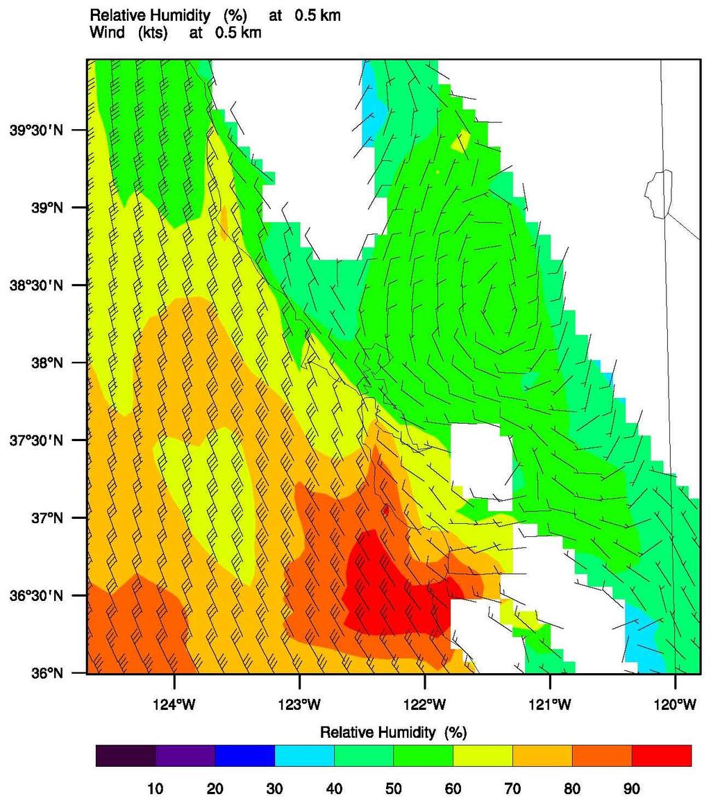
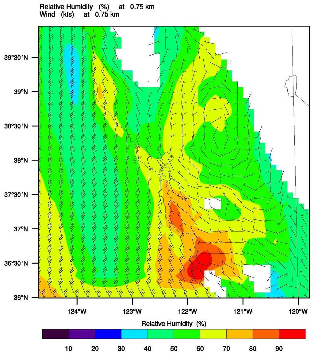
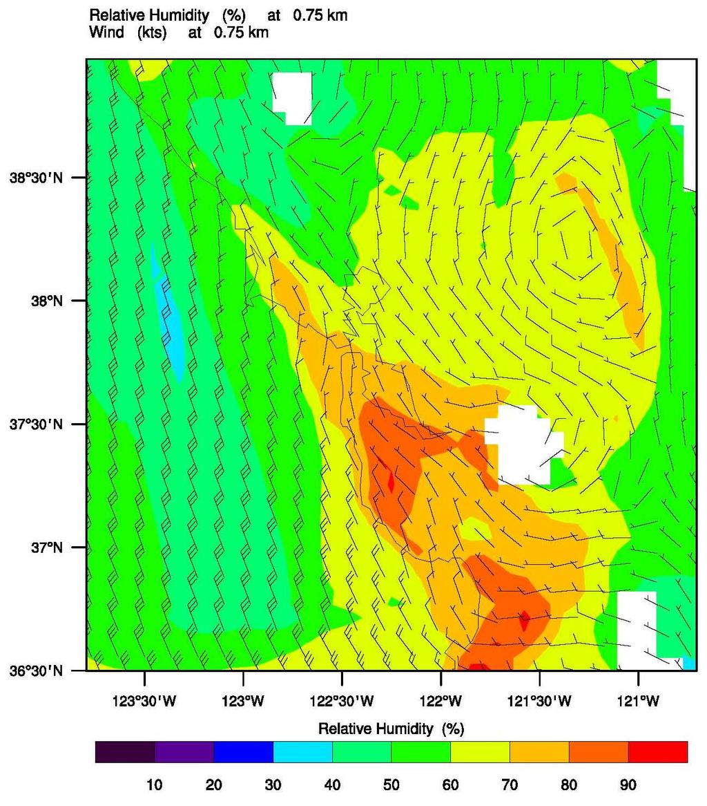
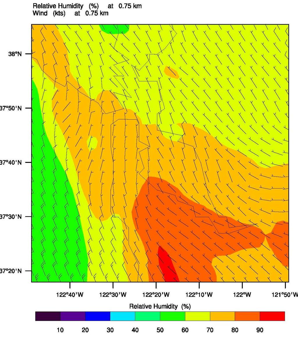
17 4.2 NCL Visualizations Relative humidity contour plots are compared to satellite images of the San Francisco Bay Area at 18Z (11am Pacic Time) for 6/21/9 and 7/11/9. Figure 8: 6/21/9 3km 17

18 Figure 9: 6/21/9 9km 18

19 Figure 1: 6/21/9 6km 19

20 Figure 11: 6/21/9 2km 2

21 Figure 12: 7/11/9 6km 21

22 Figure 13: 7/11/9 2km 5 Discussion 5.1 Simulation & Radiosonde Comparison The pressure vs. height plots show that the pressure data for the simulation agrees with the radiosonde data in all cases. This is expected, however, because 22

23 the comparisons are for total pressure which is usually very close to hydrostatic. (Variations in the horizontal are important for driving regional and local wind systems.) The 6/21/9 Z simulation data are expected to compare well with the radiosonde data because all the data are initialized using the input meteorological data, namely the NAM data at 12 km. The relative humidity of all the simulations for all four grid resolutions match the radiosonde observation data equally well. The initialization data from NAM still does not match the radiosonde data perfectly because the NAM analysis data incorporates both observations and simulations to create a best picture of the atmosphere at Z. The potential temperature simulation proles matches the radiosonde prole very well, with the exception of the 9km data, whose temperature is higher than observation at height to 5m. Likewise for wind speed: the 9km is lower compared to the rest of the simulation data. The wind direction is also least accurate for the 9km data. Given that these are all comparisons at the initial time, it is possible the grid interpolation errors are causing the dierences between the grids. The general trend of the 6/21/9 12Z data for relative humidity is captured by all the model domains. The 2km uctuates more than the rest while the 6km one ts the radiosonde data more closely. For potential temperature, the 3 and 6km data are closest to the radiosonde data while the 2km simulation data demonstrates a positive bias. For wind speed, the 3km data matches the radiosonde best, while the 2km data once again deviates most. The 2km is also farthest from the radiosonde data in the plot of wind direction, while the rest follows the radiosonde data relatively closely, indicating relatively uniform ow from the northwest. The initialization data for relative humidity for the 7/11/9 Z case do not reect the elevated humidity spikes in the radiosonde observations above m but rather show higher overall values between 1 and 2%. For potential temperature, both initialization data proles match well. Likewise for wind speed and direction there are some deviations but overall values are in good agreement. For the 12Z case of 7/11/9, the relative humidity radiosonde data shows a sudden change at height 45m, where the relative humidity jumps from to 6% indicating layering of dry and moist air. The two simulations fail to capture these sharp transitions, which may be due to poor grid resolution at these elevations. Although both are bad, the 6km case does a better job than the 2km case in that it has the same general shape as the radiosonde data. For potential temperature, both simulations do a great job but the 6km data is slightly better than the 2km near the ground. For wind speed, the 6km case again does better. However, both are not as close to the radiosonde data as desired. Similarly, wind direction is slightly better portrayed by the 6km case. Based on these results, the 3 and 6km cases seem to perform best for both days. In the 6/21/9 case, the 9km is least accurate. This suggests that maybe the grid resolution is too large to capture details observed in the Oakland radiosonde data. In the 6/21/9 case, the prediction at 12Z is more accurately portrayed by the 3km, although the 6km case is pretty close as well. The 2km 23

24 case (which was nested within the 6km grid) does not do well. This is also true in the 7/11/9 case, where the 6km grid resolution clearly does a better job than the 2km grid resolution. This could mean that the 2km is too ne a grid resolution given the parameterizations chosen, but it is likely to be more complicated than that given that two-way nesting is used. It is possible that the domain size of the 2km grid is too small, despite the fact that the 2km grid is nested within the 6km domain, which supposedly feeds more detailed lateral boundary conditions provided by the 6km domain. It is also possible that the choice of turbulence or cumulus parameterizations is no longer valid on the 2km grid. The results of the radiosonde comparison reveal the need to nd a grid resolution range that can best reproduce actual weather phenomena. The data presented suggests that the range of 3-6km surpasses the other grid resolutions chosen here in simulating weather in the Bay Area. Further simulations should be done to further pinpoint a grid resolution in the range of 3 to 6km that can product results better than the 3km or 6km horizontal grid resolutions. 5.2 Relative Humidity and Satellite Image Comparison Fog or clouds normally form when the relative humidity is at or near 1%. The color red is used to represent 1%, therefore any area of red is perceived to be cloudy or foggy. The 6/21/9 18Z (11am) contour plots show a small section of high relative humidity over lower west of San Francisco and the coastal range at the 25m level. At the 5m level and 75m level, the levels reduce to an even smaller section. The satellite image shows a clear sky over the Pacic Ocean, a hint that coastal fog has not formed or has dissipated. This implies that coastal fog has not moved into the Bay Area. The 9km and 6km case show a Pacic Ocean that has a relative humidity of 8-9%. Although there is no fog, the relative humidity is high. The 2km case has a longer patch of 1% relative humidity along the coast. From observation it is dicult to say which resolution performed best, because the satellite image shows relatively clear sky and any level of relative humidity of less than 1% cannot be seen. The 7/11/9 18Z (11am) satellite image shows white clouds along the Pacic Ocean to the west of the Bay Area, most of San Francisco and some part of Berkeley. Both the 6km and 2km cases show a large section of 1% relative humidity at the 25m level (but not at the 5m or 75m), implying that there is high possibility that fog formed. In accordance with the satellite image, the simulations show that fog is present throughout the Pacic coast and along the coastlines, the San Francisco peninsula and part of Berkeley. Both the 6km and the 2km case predict fog over most of the Bay as opposed to mainly North Bay as seen by the satellite image. This may be due in part to the representation of the topography of the coastal mountain range which serves to block and channel fog through the Golden Gate pass. 24

25 5.3 General Remarks While more simulations should be done, the study strongly suggests that 3-6km resolution grids generally outperform larger grids (such as 9km) and smaller grids (2km) in prediction of meteorological variables such as potential temperature, relative humidity, wind speed and wind direction. In the 7/11/9 case, the 6km grid resolution consistently produces better results in all categories and in the prediction of fog. Even though 2km is a ner grid resolution and has the benet of detailed lateral boundary conditions, its prediction is not as good as that of the 6km. In the 6/21/9 case, 6km and 3km grid resolutions produce the best results in the prediction of the meteorological variables. Further studies should be done that involve grid resolutions between 3 and 6km with a full exploration of physical parameterization choices to determine the ideal resolution for this region. Future studies should incorporate higher vertical grid resolution to provide more data points between and 6m height. This will provide better results in the atmospheric boundary layer where sharp gradients often exist which are not captured on coarse vertical grids. Although the physical parameterizations were held constant for all cases, one parameter that might have negatively aected the results at higher resolution is the cumulus parameterization option (cu_physics). At 2 or 3km, the cumulus scheme isn't needed. The cumulus scheme represents sub-grid scale vertical uxes and rainfall caused by convective clouds and isn't need if the grid size is small enough to explicitly resolve such motions (such as in the 2 or 3km case). This may be one explanation to why the 2km performed poorly against other horizontal grid resolutions. Another possible object of further study is nesting options. Two way nesting supposedly provides improved lateral boundary conditions to the nested domain. In the case of the 6km and 2km nest, the parent domain performed much more accurately than the nested domain. This raises questions as to how nesting aects grids of such resolution. A good alternative would be to do a two way nesting for the 9km case with a nested 3km grid resolution to compare whether or not nesting aects the accuracy of the simulation. Another possibility is to run the 2km and the 6km alone without nesting and compare the results with the nested 6km/2km case. 6 Conclusion WRF is used to simulate mesoscale atmospheric ow over the San Francisco Bay Area. Weather for 6/21/9 is modeled from Z to 18Z using ner resolutions than what are typically used for weather forecasting: 9km and 3km individually, and 6km with a two-way nest of 2km. 7/11/9 weather is modeled from Z and 18Z for the 6km resolution and its two-way nest of 2km. The goal of the simulations using ne resolutions is to determine horizontal grids that can best represent the microweather of the Bay Area and incorporate complex ter- 25

26 rain eects. Data for pressure, relative humidity, potential temperature, wind speed and direction from all simulations are plotted against radiosonde data for comparison. The 3km and the 6km horizontal grid resolutions provide most accurate simulations as compared to the radiosonde observations. The 2km grid resolution performed least accurately. Further studies should access the dierent options in nesting and parameterization as well as the vertical grid resolution to determine the potential eects they may have on the precision of simulations with various horizontal grid resolutions. 7 Acknowledgements Many thanks are due to my professor, Dr. Tina Katopodes Chow, of the Department of Civil and Environmental Engineering at the University of California at Berkeley for her patience, support and guidance throughout this research project. I am grateful for my graduate mentors, Bowen Zhou and Megan Daniels, for their consistent help with setting up the models and answering questions throughout this internship. I would also like to thank the Environmental Fluid Mechanics Research Group at UC Berkeley for all the bits and pieces I've learned from everyone and for their hospitality and accommodation. References [1] NCAR et al, 28: A Description of the Advanced Research WRF Version 3 < Chapter 1,7. [2] NCAR et al, 29: ARW Version 3 Modeling System User's Guide. < [3] Chow, F.K., A.P. Weigel, R.L. Street, M.W. Rotach and M. Xue, 22: High-Resolution Large-Eddy Simulations of Flow in a Steep Alpine Valley. Part I: Methodology, Verication, and Sensitivity Experiments. Journal of Applied Meteorology and Climatology., 45, [4] Lundquist, J.K., F.K. Chow, J.D. Mirocha and K.A. Lundquist, 27: An Improved WRF for Urban-Scale and Complex-Terrain Applications. American Meteorological Society's 7th Symposium on the Urban Environment, paper [5] White, F.M., 26: Fluid Mechanics, 4e. Mc-Graw Hills, Chapter 4. [6] Crowe, C.T., D.F. Elger and J.A. Roberson, 21: Engineering Fluid Mechanics, 7e. John Wiley & Sons, Chapters 4-7. [7] Cengel, Y.A., 1998: Heat Transfer: A Practical Approach. Mc-Graw Hills, Chapters

27 [8] Ahrens, C.D., 1991: Meteorology Today, 4e. West Publishing Company, Chapters 7-8. [9] NCL website, < 27