OCEAN CLIMATE INDICATORS STATUS REPORT 2013

Transcription

1 OCEAN CLIMATE INDICATORS STATUS REPORT 213 Meredith Elliott and Jaime Jahncke California Current Group Point Blue Conservation Science 382 Cypress Drive # 11 Petaluma, CA, il Point Blue Conservation Science

2 Acknowledgments We would like to thank our partners at Cordell Bank National ine Sanctuary (Dan Howard and Danielle Lipski) and Gulf of the Farallones National ine Sanctuary (ia Brown and Jan Roletto). We also acknowledge U.S. Fish and Wildlife Service and the Farallon National Wildlife Refuge (Anne Morkill and Gerry McChesney) for partnering with Point Blue to monitor wildlife on the Farallon Islands, California Department of Public Health (Gregg Langlois) for contributing phytoplankton data, the Institute of Ocean Sciences (Moira Galbraith) for helping process zooplankton samples collected during ACCESS cruises, and Ben Saenz for helping process the acoustics data. Funders of the ACCESS Partnership include Elinor Patterson Baker Trust Fund, Boring Family Foundation, California Sea Grant, California Dept. of Fish and Wildlife, Cordell ine Sanctuary Foundation, DJ&T Foundation, Farallones ine Sanctuary Association, Faucett Catalyst Foundation, Firedoll Foundation, Hellman Family Foundation, McCaw Family Foundation, Moore Family Foundation, National Fish and Wildlife Foundation, Oikonos Ecosystem Knowledge, Resources Legacy Fund Foundation, Restoration Center (NOAA), and Point Blue Anonymous Donors. Results in this report would not be possible without Point Blue staff, interns and volunteers. Any reference to or use of this report, or any portion thereof, shall include the following citation: Elliott, M. L. and J. Jahncke Ocean Climate Indicators Status Report 213. Unpublished Report. Point Blue Conservation Science, Petaluma, California. Point Blue contribution number For further information contact the director of the California Current Group at or Point Blue Conservation Science, 382 Cypress Drive #11, Petaluma, CA,

3 Executive Summary Physical ocean climate indicators illustrated strong upwelling in the region for the early months of 213, while a relaxation event was observed mid-year. Sea surface temperatures were cold during most of the year, with warmer surface waters in summer and early fall. Sea surface salinities were high through il, followed by declining salinities for the remaining months. Sea surface heights were anomalously low through y then appeared to rise for the rest of the year. Strong alongshore winds and positive upwelling indices during the first half of the year also confirm the strong upwelling in the region, which has translated to an early spring transition date for 213. Climate variables showed mixed results for 213. The Southern Oscillation Index (SOI) showed mostly warm water conditions for the year, with a period (ch-y) of cold water; these results likely reflect the ENSO-neutral conditions observed at the broader basin scale. The Pacific adal Oscillation (PDO) values indicated cold water conditions for the North Pacific Ocean, while the North Pacific Gyre Oscillation also showed cold, productive waters (although less productive than in recent years). Biological ocean climate indicators echo results from the physical indicators. Starting at the base of the marine food web, we found phytoplankton abundance (as indicated by chlorophyll a concentrations) appeared highest during the early and latter parts of the year, coinciding with upwelling. The phytoplankton community consisted almost entirely of diatoms, which is a good indicator of productive ocean conditions. Zooplankton community composition results are not yet available for 213. Results from the last two years (which had relatively similar ocean conditions to 213) illustrate the effects of productive ocean conditions on overall zooplankton abundance, with increased zooplankton abundance compared to warm, poor productivity years (e.g. 24-6), particularly for euphausiids and copepods. Analyses of zooplankton samples show two main clusters: the first three years (24-6), and the next five years (27-11). Results on various mid-trophic level species are not available for 213. Copepod community composition results to date indicate large increases in the abundance of boreal copepods (i.e., species from northern latitudes which are generally considered better prey based on their larger size and greater lipid content) during cold, productive ocean conditions. Copepod species common to mid-latitudes also became more abundant in cold water years, although not as dramatically. Equatorial copepods (i.e., copepods from southern latitudes which are smaller and have less lipid content) increased in abundance in the tember cruises some years. Pteropod abundance has remained relatively low throughout our time series, with significant increases in

4 211. Euphausiid biomass results (as measured by acoustics) indicate a peak in krill densities in y 213; over time, there appears to be declining krill abundances since 29. Adult krill, which are larger and higher in lipid content than their younger counterparts, dominate the zooplankton samples during cold water years, including 213; however, the percentage of adult stages appears to be declining since mid- 21. The top-level predators in our region are represented by three resident breeding seabirds and two migrant whales. Cassin s auklet, a zooplanktivorous seabird, was observed foraging on the shelf and near the shelf break in 213; this species began breeding slightly early this year on SEFI and experienced high productivity. An omnivorous seabird species, the common murre, foraged more in nearshore waters and on shelf waters near SEFI in 213, had an early start to breeding, experienced average breeding success, and fed mostly on rockfish. Brandt s cormorants are piscivorous and were observed in low numbers near SEFI and in nearshore waters in 213. This species had a slightly early start to breeding, experienced very high productivity (contrary to recent years of low breeding success), and consumed mostly rockfish species in 213. For marine mammals in 213, humpback whales were observed in higher numbers in the y and tember cruises, and they were spotted on the shelf and near the shelf break. Blue whales peaked in abundance in tember 213 and were observed mostly on the shelf break, with a few sightings on the shelf.

5 Introduction The Applied California Current Ecosystem Studies (ACCESS) is a partnership between a science organization and a Federal agency to inform management in support of marine wildlife conservation in central California, encompassing NOAA National ine Sanctuary waters (CBNMS, GFNMS and MBNMS) and the potential expansion area south of Point Arena, in Federal and State waters (Figure 1). Our group has initiated integrated, collaborative, and multi-disciplinary research to monitor distribution, abundance and demography of marine wildlife in the context of underlying physical oceanographic processes. We are also working towards coordinated private and government research at an ecosystem scale to support a healthy marine ecosystem in the region. Effective management and conservation of natural resources requires adaptive management strategies that are informed by robust analysis of past and present data, which we intend to provide in this report. Some of the main potential issues we aim to address include 1) water quality (ecosystem effects of freshwater outflow), 2) ocean zoning (guide human uses to provide protection of the marine ecosystem), 3) climate change (document effects of environmental change on the marine ecosystem), 4) fisheries (contribute to ecosystembased management approaches), and 5) water quality (assess ecosystem effects of freshwater outflow). The information we collect, while available upon request, will become available to collaborators as part of the California Avian Data Center ( The purpose of this report is to inform managers and policy-makers about wildlife responses to changes in ocean conditions and to mobilize public support for conservation. This effort builds off the report Ocean Climate Indicators: A Monitoring Inventory and Plan for Tracking Climate Change in the North-central California Coast and Ocean Region ( Monitoring-Plan-FINAL.pdf), which was used to help prioritize indicators to include in the Point Blue report, but additional indicators were also included, as these data were readily available and provide a more comprehensive picture of regional ocean conditions. We have compiled a variety of datasets to look at long-term trends, as well as short-term trends (i.e., 24-present). While some datasets have been updated through this year, not all 213 data are available. We have shown here what we could obtain at the time we released this report.

6 Figure 1. Applied California Current Ecosystem Studies (ACCESS) study area.

7 Sea surface temperature Overview Sea surface temperature (SST) is a way of monitoring the productivity of the ecosystem, as cold water is brought to the surface during upwelling in early spring. The surface waters eventually warm up during relaxation events that follow upwelling, typically in late summer or early fall. We used buoy and Southeast Farallon Island data for more localized observations, and satellite data were used for a more regional perspective on SST. Buoy data SSTs in 213 were anomalously cold (i.e. large negative blue bars) for most months, with the exception of - when SSTs were closer to the long-term mean (Figure 2). SSTs were close to average values in the early months of 24. In 25 and 26, anomalously warm SSTs (i.e. large positive red bars) were observed in the winter and spring months. In contrast, low SSTs were noted in most months of years 27-12; short periods of average or warm waters (e.g. late months of 28, early months of 21) suggest local downwelling/relaxation events. Southeast Farallon Island data SST data collected near Southeast Farallon Island (SEFI) shows similar results for 213, with cold (i.e., negative blue bars) temperatures dominating the year but with warmer (i.e., positive red bars) temperatures observed later (-) than the buoy results (Figure 3). There were some signs of short upwelling events in 24, but most values were closer to the long-term averages. Warm SSTs were observed throughout most of Conversely, cold SSTs were observed throughout the early months of Results for 21 suggest delayed upwelling in that the cold temperatures were not noticed until il and. SSTs in 211 were normal to warm for most of the year, then SSTs dropped in 212. Satellite data Satellite results show cooler (i.e., negative blue bars) SSTs in 213 in spring (-) and fall (), while a relaxation event may have occurred during summer (-; Figure 4). Temperatures in 24 through mid-25 were consistently warm (i.e., positive red bars); this differs from the buoy and SEFI data, as these other data show periods of cold, upwelled water at the surface. Similar to buoy and SEFI results, 26 had warmer SSTs in the first half of 26, and cold SSTs in the first half of years Warm waters in the early months and cold waters in the later months of 21 are also consistent with other SST results. SSTs in 211 were average, while 212 showed mostly cooler SSTs.

8 Jan Jan e il t y Monthly anomalies Jan Jan e il Jan Jan Data source: with additional data from: Figure 2. Monthly anomalies of SSTs, Bodega buoy, Black lines represent ±99% confidence intervals around the long-term monthly means. Monthly anomalies Data source: Monthly anomalies Figure 3. Monthly anomalies of SSTs, SEFI, Black lines represent ±99% confidence intervals around the long-term monthly means Data source: Figure 4. Monthly anomalies of SSTs, MODISA satellite, Black lines represent ±99% confidence intervals around the long-term monthly means.

9 Sea surface salinity and height Overview Other variables used to estimate upwelling and productive oceanographic conditions are sea surface salinity and sea surface height. Higher salinity values can be a sign of nutrient-rich waters, which is a result of upwelling. During upwelling, surface waters along the coast are pushed offshore, causing depressed sea surface heights near the coast; the opposite is true for downwelling conditions, as offshore water returns to the coast and causes a rise in sea surface height. Southeast Farallon Island data Sea surface salinity data from SEFI in 213 shows high salinity values (i.e. the positive blue bars) in the early months, suggesting upwelling, then progressively lower salinity values (i.e. the negative red bars) for the rest of the year (Figure 5). Low salinity values were evident in 24-6, indicating weak upwelling conditions. Anomalously high salinity values were observed in early months of 27-9 and 212. Salinity values in were average, indicating a lack of strong upwelling events in the early months of these years. Satellite data Sea surface height in 213 was lower (i.e., negative blue bars) in spring-summer (- ), suggesting upwelling conditions during this period; then downwelling conditions (i.e. positive red bars) were observed for the remainder of the year (Figure 6). In general, sea surface heights were higher than average in 24-6, indicating downwelling or relaxation conditions. From early 27 through the first half of 29, sea surface height declined, suggesting upwelling in the region. Conditions switched in mid-29 to higher sea surface heights (i.e., downwelling), then switched again in mid- 21 to lower surface heights, which persisted through ruary 211. Weak relaxation conditions returned in - 211, then weak upwelling conditions dominated the remainder of the year and into 212. Weak upwelling was followed by weak downwelling starting in 212 and for the rest of the year.

10 Jan Jan Jan Jan 1 Monthly anomalies Data source: Figure 5. Monthly anomalies of sea surface salinity, SEFI, Black lines represent ±99% confidence intervals around the long-term monthly means. Monthly anomalies Data source: Figure 6. Monthly anomalies of sea surface heights, Aviso satellite, Black lines represent ±99% confidence intervals around the long-term monthly means. NOTE: Data have been re-formatted starting in y 29; therefore, anomalies and confidence intervals before y 29 are different than anomalies and confidence intervals since y 29.

11 Winds, upwelling and spring transition Overview Upwelling is a wind-driven process where coastal winds blowing parallel to the coast result in an offshore movement of surface water drawing deep, cold, nutrient-rich waters to the surface nearshore. The strength and timing of upwelling can have significant effects on the marine ecosystem. In addition, periods of strong upwelling should be alternated by relaxation events to allow for the spring bloom to occur. Winds Alongshore winds in 213 were particularly strong (i.e. negative blue bars) in Jan-; winds relaxed in - (i.e. positive red bars), followed by moderate winds to strong winds for the rest of the year (Figure 7). There was moderate alongshore wind activity in 24, followed by a lack of alongshore winds in Strong, upwellingproducing winds are clearly visible in the early months of Alongshore winds in 21 appeared to weaken, with some strong wind activity in - and. Winds continued to be moderate to weak throughout most of , with periods of stronger winds observed in the early and later months of these years. Upwelling Strong upwelling conditions (i.e. positive blue bars) dominated most of 213, with a few months (e.g.,, and ) of reduced upwelling (Figure 8). Intermittent upwelling and downwelling (i.e. negative red bars) events were noticed in the early months of some years (e.g. 24, 211), while upwelling was weak and delayed in 25-6 and 21. Strong upwelling conditions were found in the early months of 27-9, followed by relaxation events. Strong upwelling was noted in 212, with downwelling occurring in early and late parts of that year. Upwelling indices calculated from buoy data are similar to the regional results for 213, but they capture the more localized periods of relaxation in the middle of the year not observed in the monthly indices (Figure 9). Spring transition The spring transition date for 213 was ruary 21, the second earliest transition date in the time series (Figure 1). Most of the recent years (e.g. 26-9) showed earlier transition dates (i.e. negative red bars) and some years (e.g. 21) had a late spring transition (i.e. large positive bars). Spring transition dates calculated from Bodega Bay buoy data since 1981 show similar results as dates calculated from upwelling indices for most years, including a very early date for 213 (Figure 11). Late transition dates tend to be associated with El Niño events (e.g. 1983) and early dates with La Niña years (e.g., 27).

12 Monthly anomalies Jan Jan Jan Jan Jan Jan Data source: Figure 7. Monthly anomalies of alongshore winds, Black lines represent ±99% confidence intervals around long-term monthly means. Monthly anomalies Data source: Figure 8. Monthly anomalies of upwelling indices, Black lines represent ±99% confidence intervals around long-term monthly means. 1 Data source: Monthly anomalies Figure 9. Monthly anomalies of upwelling indices as calculated from the Bodega buoy data, Black lines represent ±99% confidence intervals around long-term monthly means.

13 Annual anomalies Data source: Figure 1. Anomalies of spring transition dates based on daily upwelling indices, Black lines represent ±99% confidence intervals around 42-year mean. Annual anomalies Figure 11. Anomalies of spring transition dates based on Bodega Bay buoy data, Black lines represent ±99% confidence intervals around 33-year mean.

14 Climate Indices Overview Several climate variables have been developed to understand climate effects on the basin-level scale. The Southern Oscillation Index (SOI) uses differences in mean sea level pressure anomalies between Tahiti and Darwin, Australia. Negative SOI values indicate warm ocean conditions related to El Niño, and cold water conditions are shown in positive SOI values. The Pacific adal Oscillation (PDO) shows changes in surface waters in the North Pacific (from 2 N to the pole) at inter-decadal scales. Positive PDO values correspond to warmer ocean waters in the eastern Pacific, and negative PDO values correspond to cold waters. The North Pacific Gyre Oscillation (NPGO) measures changes in circulation of the North Pacific gyre, and is highly correlated with nutrients and overall productivity. Similar to the SOI, negative NPGO values reflect warm water and poor productivity, while cold water and high productivity correspond to positive NPGO values. Southern Oscillation Index (SOI) SOI values in 213 showed mildly warm water conditions (i.e. negative red bars) early and late in the year and colder conditions (i.e. positive blue bars) in - (Figure 12). Warm water conditions were observed from 24 through the first half of 27. SOI values showed cool water conditions from mid-27 through early 29, at which point the SOI changed to negative values again. The SOI remained mostly negative throughout the later months of 29 and early 21, switching to positive values in ch 21. SOI values in 211 showed largely cold water conditions, while values in 212 were average to warm. Pacific adal Oscillation (PDO) PDO results for 213 showed cold water conditions (i.e. negative blue bars) for most of the year, although some months (e.g. Jan, -, ) were close to average (Figure 13). Warm water conditions (i.e. positive red bars) dominated the early years of this time series (roughly 24-7), while cold water conditions were more prominent from late 27 through the end of 29. A brief period of warm water conditions returned in late 29 and early 21, then giving way to cold conditions from mid-21 to the present. North Pacific Gyre Oscillation (NPGO) NPGO values for 213 show cold, productive ocean conditions (i.e. positive blue bars), although not as cold and productive as recent years (Figure 14). Warm water, poor productivity conditions (i.e. negative red bars) were observed throughout 25 and 26. Normal values were observed for most of 29, while cold, productive conditions were evident in all other years.

15 SOI values Jan Jan Jan Jan Jan Jan Data source: PDO values Figure 12. Southern Oscillation Index (SOI) values, Black lines represent ±99% confidence intervals around the long-term monthly means Data source: NPGO values Figure 13. Pacific adal Oscillation (PDO) values, Black lines represent ±99% confidence intervals around the long-term monthly means Data source: Figure 14. North Pacific Gyre Oscillation (NPGO) values, Black lines represent ±99% confidence intervals around the long-term monthly means.

16 Chlorophyll a and phytoplankton composition Overview Concentrations of chlorophyll a can provide information on the amount of phytoplankton in surface waters. The timing of peak phytoplankton abundance could also have effects on how productive a marine ecosystem will be. Satellite data provide us with phytoplankton abundance estimates. Phytoplankton collected within and adjacent to the Sanctuaries was analyzed by the California Department of Health to help us understand the phytoplankton community composition. Composition of the phytoplankton community can provide insight into how productive an ecosystem might be. For instance, an increase in the abundance of dinoflagellates (a small organism) could signify poor ocean conditions, whereas a greater abundance of diatoms (a larger organism) could indicate more productive ocean waters. Satellite data Phytoplankton blooms (i.e. positive anomalies) were observed in the early months (Jan- ) and again in the fall (-; Figure 15). There is some evidence of peak chlorophyll in the spring and fall months of 24-7, but evidence for sustained phytoplankton blooms is lacking in From the oceanographic results, we might have anticipated seeing anomalously high chlorophyll a concentrations in 27-9, when upwelling conditions were good. However, blooms are known to occur after the seasonal thermocline is established, so the peak chlorophyll concentrations in later months (fall and winter) of 25 and 26 could be explained by the delayed upwelling in those years. Strong upwelling and a lack of relaxation could explain the average to low phytoplankton abundance in Blooms appeared more frequently in 211 but were relatively small and sporadic, whereas blooms were relatively non-existent in 212. California Department of Health data Phytoplankton composition in 213 was largely dominated by diatoms throughout the year, similar to 212 (Figure 16). Other years (e.g. 26, 27, 29 and 211) showed an increase in dinoflagellates from spring/summer to fall/winter, while other years (e.g. 21 and 212) showed low dinoflagellate abundance throughout the year. Dinoflagellates are most associated with warm, less turbulent waters later in the year (when diatoms sink and become scarce in surface waters) and are responsible for harmful algal blooms (e.g. red tides) common in the fall months. Contrary to most years, dinoflagellates were relatively more abundant than diatoms in the spring/summer of 28. The greater importance of diatoms (i.e., the species most associated with cold, turbulent ocean waters) throughout the eight-year time series could indicate improved upwelling conditions through time.

17 Monthly anomalies Jan Jan Data source: Figure 15. Monthly anomalies of chlorophyll a, MODISA satellite, Black lines represent ±99% confidence intervals around the long-term monthly means. Average percent composition diatoms dinoflagellates Figure 16. Average relative composition of diatoms and dinoflagellates in offshore samples,

18 Zooplankton composition Overview Information on the abundance and species composition of zooplankton are also indicators of the productivity of an ecosystem. For example, an overabundance of gelatinous species can signify poor productivity, and a highly productive ecosystem may have high abundances of euphausiids (which are important prey for fish, seabirds, and marine mammals). Relative composition While all years of data are not yet available, we can see variability in zooplankton abundance and composition in years (Figure 17). From tember 24 through ober 26, the overall average abundance of zooplankton is greatly reduced and never reaches over 3 individuals per cubic meter of water sampled. The trend changed in 27, when overall zooplankton abundance increased dramatically, and this overall increase in zooplankton abundance is sustained for most surveys in 27 and 28. This is mainly attributed to increases in euphausiid and copepod abundance. The first half of 29 shows high zooplankton abundance (especially euphausiids and copepods), followed by a return to low zooplankton densities. Results from 21 show increasing zooplankton abundances through the year, with a significant increase (particularly for copepdos) in tember. Preliminary results for 211 indicate dramatic increases in all zooplankton, especially euphausiids. Community analysis We looked for similarities between different years based on the zooplankton data by performing a non-metric multi-dimensional scaling analysis for samples collected in the spring and summer months (-; Figure 18). In general, there appear to be two main groups that cluster together: years 24-6, and years

19 Average abundance (# / m 3 ) AMPHIPODS COPEPODS DECAPODS EUPHAUSIIDS MYSIDS PISCES Other Figure 17. Zooplankton composition in the upper 5 m of the water column determined from hoop net samples, NOTE: Euphausiid abundances include all life stages except eggs. Figure 18. Non-metric multi-dimensional scaling analysis of zooplankton results, - samples, NOTE: Data are not complete for 211.

20 Copepods Overview Copepods are mid-trophic level organisms, and they are the most abundant and diverse zooplankton taxon, constituting the largest source of protein in the marine environment. Copepod communities change in response to changing oceanographic conditions, and the presence and absence of key species can indicate these changes. Copepods that are common to northern latitudes (called boreal species) become more abundant in colder, productive ocean waters. Transition zone species are common species to this region, yet they can become more abundant in colder waters and less abundant in poor ocean conditions. Equatorial species (i.e., species from tropical or subtropical regions) can be found during warm water intrusions (e.g., El Niño events) from southern latitudes. Relative composition While we do not yet have data for all years, the results we do have indicate changes in the copepod species composition, the most notable in the boreal species (Figure 19). These species were largely absent for the first three years of data (24-6), and abundance increased significantly in 27-8; boreal species declined again in the latter half of 29, but a dramatic increase was observed in 21 and preliminary data for 211. Species common to mid-latitude areas were in relatively low abundances throughout the time series, with peaks in abundance in the latter months (especially tember) in 27-8 and 21 (Figure 2). Equatorial copepods remained in low abundances throughout the eight years, except for the increases in abundance during tember cruises of 27-9, and an apparent increase in y 211 (Figure 21).

21 Average abundance (# / m 3 ) Figure 19. Average abundances of boreal copepod species, NOTE: Data are not complete for 211. Average abundance (# / m 3 ) Figure 2. Average abundances of transition zone copepod species, NOTE: Data are not complete for 211. Average abundance (# / m 3 ) Figure 21. Average abundances of equatorial copepod species, NOTE: Data are not complete for 211.

22 Pteropods Overview Pteropods are pelagic marine gastropods and are commonly known as sea butterflies. There are two orders of these mid-trophic level organisms: Thecosomata and Gymnosomata; the former contains a shell while the latter does not. One species belonging in the order Thecosomata, Limacina helicina, has been used to study the effects of ocean acidification. This species calcium carbonate shell is sensitive to dissolution in acidic conditions, and shell thickness can be measured on this species to assess ocean acidification and its effects on the marine environment. L. helicina has been classified as a key indicator species of ocean acidification. Abundance We do not yet have results from 213. However, results to date have revealed very low abundances of L. helicina in our region, particularly in the first two years (Figure 22). Increases were first noted in 26 (which may have coincided with the beginning of the delayed upwelling in that year). Abundances have remained at low levels since, with dramatic increases noted in the 211 cruises. The significance of these results so far are still being discussed. Future work is being planned to measure the shell thickness of this species from the ACCESS cruise samples. Average abundance (# / m 3 ) Figure 22. Average abundance of the pteropod Limacina helicina, NOTE: Data are not complete for 211.

23 Euphausiids Overview Euphausiids (commonly known as krill) are important mid-trophic level organisms, feeding mainly on phytoplankton and then becoming prey for many marine top predators (e.g., salmon, seabirds, and humpback whales). There are two main species found in the Gulf of the Farallones: Euphausia pacifica and Thysanoessa spinifera, the former being more abundant than the latter. Adult and immature stages of these species are known to be the primary prey items of the Cassin s auklet, a zooplanktivorous seabird species breeding on the Farallon Islands. Abundance Acoustic biomass results of euphausiids down to 2 m below the surface in 213 reveals similar results to 212: a peak in biomass in y and lower biomass observed in the earlier and later months (Figure 23). Lower abundances of krill were observed in 24-8 (with seasonal peaks in spring/summer), followed by increases in 29-11; while higher biomass was noted in compared to the early years of this time series, krill abundance appears to be slowly declining. Annual peaks in euphausiid abundance appear to happen mostly during y cruises in the latter years of our time series. The large 26 densities are likely due to salps and other gelatinous zooplankton that were abundant that year, as these species can confound acoustic results. Euphausiid age classes Adult E. pacifica were more abundant in Tucker trawl samples (i.e., sampling down to 2 m) during the and y cruises of 213, then younger life stages became slightly more abundant in tember (Figure 24). Adult krill were more abundant during the cold, productive conditions of 27-8, as well as average conditions in 21-11, while younger stages dominated during the warm, less productive conditions observed of 25-6 and the latter part of 29. Adults were abundant for most of 21-12, although percentages appear to be declining through time. Fall cruises (tember) usually show higher percentages of the younger life stages.

24 Average density of euphausiids (g/m 2 ) Figure 23. Acoustic biomass of euphausiids down to 2 m, Percent of total wet weight zoea juveniles immatures adults Figure 24. Percent composition of different age classes of Euphausia pacifica,

25 Birds Overview Seabirds are top marine predators that feed on a variety of marine organisms. Some species breed within our study area, while other species migrate great distances to spend their non-breeding period in the central California Current. The abundances and distributions of marine birds have been linked to bathymetric and hydrographic features which aggregate prey; many seabirds live in or travel to the central California Current because of the highly-productive waters common to the region. Relative composition There were a total of 55 species of seabird identified during at-sea cruises (Table 1). When looking at the top ten most abundant seabird species, six of these are known to breed on SEFI or other areas within the central California Current. Sooty and pinkfooted shearwaters overwinter in the study area, while phalarope species can be found here as they make their way from their Arctic breeding grounds to tropical waters for the non-breeding period. The next few sections will concentrate on the information available on some of these abundant species, particularly three species which breed on SEFI: common murre, Cassin s auklet, and Brandt s cormorant.

26 Table 1. Seabird species and average densities per cruise, Average density (number of animals observed per km 2 of survey area) Average density (number of animals observed per km 2 of survey area) Common Name Common Name common murre Canada goose.1133 Cassin's auklet 9.97 unidentified duck.1133 sooty shearwater peregrine falcon.1133 western gull parasitic jaeger.1132 Brandt's cormorant Thayer's gull.1132 rhinoceros auklet.9442 unidentified loon.1132 unidentified phalarope.6372 mottled petrel.137 red-necked phalarope.657 red-throated loon.137 pink-footed shearwater.4751 black scoter.999 California gull.3663 black storm-petrel.884 northern fulmar.349 herring gull.644 black-footed albatross.2581 pigeon guillemot.2151 red phalarope.1884 fork-tailed storm-petrel.158 unidentified gull.1227 Buller's shearwater.976 Heermann's gull.596 unidentified shearwater.525 ashy storm-petrel.51 black-legged kittiwake.396 pelagic cormorant.258 brown pelican.238 tufted puffin.18 Pacific loon.165 Sabine's gull.151 Bonaparte's gull.142 unidentified alcid.138 unidentified dark shearwater.125 Scripps's murrelet.117 short-tailed shearwater.96 pomarine jaeger.88 Arctic tern.77 surf scoter.58 unidentified auklet.54 double-crested cormorant.39 flesh-footed shearwater.34 glaucous-winged gull.33 ancient murrelet.32 common loon.25 elegant tern.23 unidentified storm-petrel.21 Laysan albatross.16 South Polar skua.12

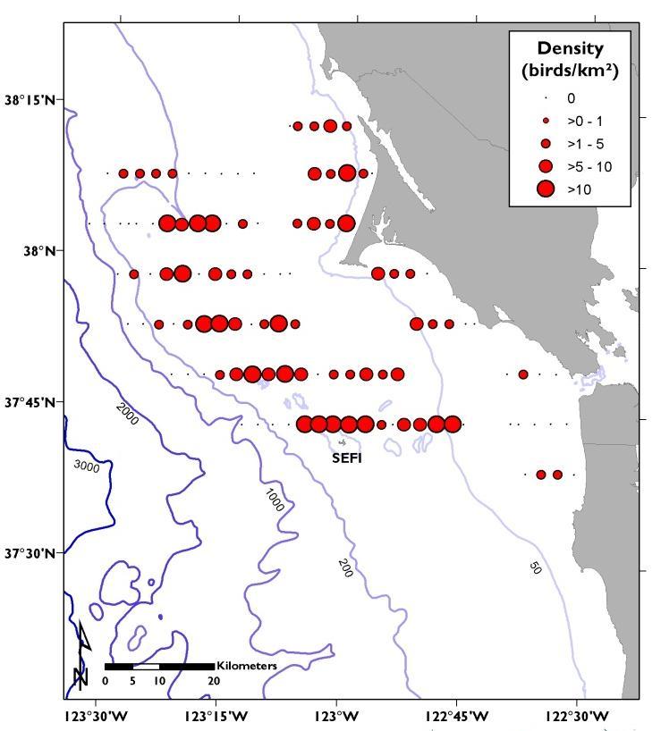
27 Cassin s auklet Brief species account The Cassin s auklet is a small burrowing seabird that breeds on the Farallon Islands. This is a zooplanktivorous species, with the majority of their diet consisting of euphausiids. Abundance In 213, the highest number of Cassin s auklets (852 auklets) was observed in y (Figure 25). The highest number of Cassin s auklets in the time series was found in 24 (2683 auklets). After this, less than half this peak number was observed in any cruise. In general, counts were higher during the breeding season (ch-ust). The lowest number of auklets was found in 26, the year with delayed and weak upwelling conditions. Numbers rebounded to some degree in 29-12, with peak numbers occurring in y or tember in these years. Total number observed Figure 25. Abundances of Cassin s auklets observed during each cruise, Distribution Cassin s auklets were observed near the Farallones and north along the shelf break during and e in most years, including 213 (Figure 26). Cassin s auklets are raising chicks during the months of and e, which is why they were found close to SEFI in some years (e.g., 212). While not shown here, poor upwelling years (e.g. 25-6) were characterized by smaller auklet flocks, and they ventured farther north and inland. Improved ocean conditions returned in 27, and auklets were observed over Cordell Bank, along the shelf break and closer to SEFI, but not in the large flocks noted in 24.

28 Figure 26. Cassin s auklet distributions during or e

29 Cassin s auklet Timing of breeding The Cassin s auklet median egg lay date for 213 was slightly earlier than the 42-year average on SEFI (Figure 27). Anomalously late lay dates correspond to El Niño events (e.g., 1982, 1992, 1998), when ocean conditions were poor. Since 24, lay dates for Cassin s auklets have been average or earlier than the long-term average, with only 25 (i.e., a poor ocean condition year) being later. There is a slight trend towards later lay dates through the time series, but this is not significant. Breeding success Breeding success for the Cassin s auklet on SEFI was anomalously high in 213, plotting well above the 43-year mean, lying at the upper 8% confidence interval (Figure 28). The anomalously low productivity years have occurred during El Niño years (e.g., 1983, 1992) and generally correlate with years of later egg laying (Figure 27); years 25 and 26 are exceptions, as these were not El Niño years and lay dates were near the average, but they were the worse productivity years on record. Conversely, earlier lay dates (e.g., 29-11; Figure 27) were linked to better productivity, indicating that an earlier start to breeding can lead to higher breeding success. Diet The diet of the Cassin s auklet in 213 was dominated by euphausiids, as in most years of the 32-year time series (Figure 29). The diet in 25 and 26 deviate greatly from the other years, as mysids (shrimp-like marine invertebrates) comprised the entire diet of the few diet samples collected in those years. This also led to breeding failure (Figure 28), revealing the importance of krill in this species diet, as well as the lack of krill in the region during 25 and 26. Since the breeding failures of 25-6, euphausiids have increased in the auklet diet, and breeding success has also rebounded.

30 Standardized anomaly (days) Figure 27. Cassin s auklet annual median egg lay dates on SEFI, Standardized productivity anomaly Figure 28. Cassin s auklet breeding success anomalies on SEFI, Solid black line represents 43-year mean, and dotted red lines represent ±8% confidence intervals. Percent by number 1% 8% 6% 4% 2% % Other Pisces Mysids Amphipods Euphausiids Figure 29. Cassin s auklet diet composition on SEFI,

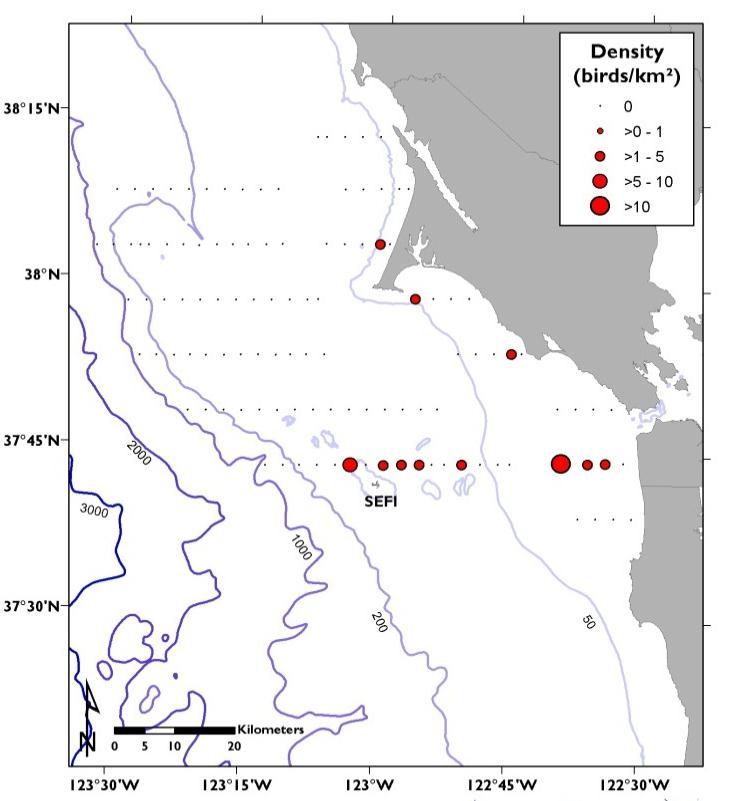
31 Common murres Brief species account The common murre is a frequently-observed seabird in the Gulf of the Farallones and breeds on the Farallon Islands. They are an omnivorous seabird feeding mainly on fish, but they also consume zooplankton. Abundance In 213, common murres were observed in slightly higher abundances compared to 212, with the highest number counted in y (Figure 3). Since 24, the highest number of murres were seen in y 21 (245 murres) and il 25 (2264 murres). This species was abundant in 24 and early 25, then declined in abundance in 26. Counts of murres gradually increased over the next few years, followed by a decline after 21. In general, this species was present in higher number in spring and summer (i.e., the breeding months) than in the fall months. Total number observed Figure 3. Abundances of common murres observed during each cruise, Distribution In 213, common murres were observed near SEFI and northward in shelf waters, especially in the nearshore environment (Figure 31). In most years, murres have been observed in shelf waters near SEFI and between SEFI and Cordell Bank (e.g., 24-6 and 28, not shown; 21-11, Figure 31). In some years, this species was more dispersed, with more observations in the northern parts of the study area (e.g., 25 and 29, not shown) or further nearshore to the southeast area of SEFI (e.g., 27-8, not shown). Note that distributions shown here represent adult murre distributions; common murre chicks do not start appearing in the waters of the Sanctuaries until y and after.

32 Figure 31. Common murre distributions during or e,

33 Common murres Timing of breeding In 213, common murres on SEFI had a median egg laying date earlier than the 42- year mean (Figure 32). Similar to the Cassin s auklet, we observed that common murres have later lay dates in poor ocean condition years (e.g., 1983, 1992, 1998). Since 24, the annual median lay date has hovered close to the long-term mean, with some years showing earlier lay dates (e.g., 24, 27, 28) and some years showing later dates (e.g., 25, 26, 29-11). There has been a slight trend in earlier lay dates through time, although this is not significant. Breeding success Common murre breeding success in 213 was equivalent to the 42-year mean (Figure 33). Similar to the Cassin s auklet, anomalously low productivity years (e.g., 1983, 1992, 1998) that punctuate the time series correspond to El Niño years, as well as years with late median lay dates (Figure 32). However, recent years of extremely low breeding success (i.e., 26 and 29) had relatively late median lay dates but were not El Niño years. Earlier lay dates (e.g., 1988; Figure 32) were linked to better productivity in some years, but this was not consistent; annual median lay dates for 26 and 29 were earlier compared to 25, yet breeding success was worse. Some of these discrepancies in lay dates and productivity can be explained by low feeding rates to chicks, as observed in 29. Diet In 213, juvenile rockfish was the most common prey item being fed to common murre chicks (Figure 34). Prey items being brought to common murre chicks has varied over time, with rockfish being the main diet items in the 197s and 198s, then anchovy and sardine becoming the dominant prey in the 199s. This changed again in the early 2s when rockfish became the dominant prey, then back to anchovy/sardine in the 24-8 period. Since 29, rockfish has been more important in the diet. Historically, El Niño years corresponded to years with a low percentage of rockfish in the diet; these were also years of late timing of breeding (Figure 32) and low breeding success (Figure 33). However, 25 and 26 were not El Niño years, yet these years of poor ocean conditions yielded late breeding, low breeding success, and few rockfish in the murre diet. The 29 results have been exceptional, as murres were eating a lot of rockfish, yet breeding success was one of the lowest years on record; as mentioned previously, low chick feeding rates can help explain the low productivity in this year.

34 197 Standardized anomaly (days) Figure 32. Common murre annual median egg lay dates on SEFI, Standardized productivity anomaly Percent by number Figure 33. Common murre breeding success anomalies on SEFI, Solid black line represents 42-year mean, and dotted red lines represent ±8% confidence intervals. 1% 8% 6% 4% 2% % Other Anchovy/Sardine Rockfish Figure 34. Common murre chick diet composition on SEFI,

35 Brandt s cormorant Brief species account Brandt s cormorants are piscivorous birds found throughout the coastal areas of California. They are one of the seabirds monitored on SEFI. Abundance Since 28, Brandt s cormorants were observed in very low numbers, and this trend has continued in 213 (Figure 35). Numbers of Brandt s cormorants have declined through the time series, with the peak in ober 24 (273 cormorants); since this cruise, numbers have been less than half of this high count. The ober 24 peak was later in the year compared to the high counts of other years, which generally occurred during the summer months (i.e., the breeding season). The low abundances observed in correspond to poor productivity for this species in these years (Figure 38). Total number observed Figure 35. Abundances of Brandt s cormorants observed during each cruise, Distribution In 213, Brandt s cormorants were observed near SEFI and in nearshore waters near San Francisco Bay and the Point Reyes peninsula (Figure 36). Brandt s cormorants have been observed near SEFI in most other years (Figure 36). In some years, this species was more scattered and observed in smaller groups or as individual birds in waters closer to shore (e.g., 27, not shown; 21 and 212).

36 Figure 36. Brandt s cormorant distributions during or e,

37 Brandt s cormorants Timing of breeding The median egg lay date for Brandt s cormorants on SEFI in 213 was earlier than the 42-year average (Figure 37). Timing of breeding in Brandt s cormorants isn t as clearly linked to ocean conditions as in Cassin s auklets or common murres; El Niño years (e.g., 1983, 1992, and 1998) do not show anomalously late lay dates. There has been a slight trend in later lay dates through time, although this is not significant. Since 24, this species began breeding early for four years (24-7), and then bred extremely late in the following five years (28-12). Breeding success Breeding success of Brandt s cormorants on SEFI in 213 was one of the highest annual productivity values of this species in the 43-year time series (Figure 38). Most of the annual productivity estimates for Brandt s cormorants fall within the 8% confidence intervals around the long-term mean, similar to auklets and murres; however, unlike auklets and murres, Brandt s cormorants have experienced several years of extremely low productivity, usually corresponding to El Niño years (e.g., 1983, 1992). In looking at breeding success data since 24, above average breeding success was observed in the first four years (24-7), then extremely low productivity in 27-12, and now it is very high in 213. Diet Brandt s cormorants on SEFI in 213 consumed almost exclusively rockfish (Figure 39). The diet of Brandt s cormorants on SEFI has consisted of forage fishes (i.e., northern anchovy, Pacific sardine), various benthic species (i.e., sculpins, gobies, rockfish, and flatfish), and cephalopods. Years with high percentages of anchovy and sardine in the diet (e.g., 25-7) have usually corresponded to years of high productivity, with the exception of 213 (Figure 38).

38 Standardized anomaly (days) Figure 37. Brandt s cormorant annual median egg lay dates on SEFI, Standardized productivity anomaly Percent by number Figure 38. Brandt s cormorant breeding success anomalies on SEFI, Solid black line represents 42-year mean, and dotted red lines represent ±8% confidence intervals. 1% 8% 6% 4% 2% % Cephalopods Anchovy/Sardine Rockfish/Sculpin Flatfish Other Figure 39. Brandt s cormorant diet composition on SEFI, NOTE: Data for years from Ainley et al Years 1999, 24 and 26 have low sample sizes.

39 Mammals Overview ine mammals are top marine predators that feed on a variety of marine organisms. Some species breed within our study area, while other species migrate great distances to spend their non-breeding period in the central California Current. The abundances and distributions of marine mammals have been linked to bathymetric and hydrographic features which aggregate prey; many marine mammals live in or travel to the central California Current because of the highly-productive waters common to the region. Relative composition There were 31 species of marine mammals observed during at-sea cruises since 24 (Table 2). When looking at the top fifteen most abundant marine mammal species, two of these are known SEFI inhabitants: California sea lion and Steller sea lion; both of these species are piscivorous. Risso s dolphin, Dall s porpoise, northern right whale dolphin, and Pacific white-sided dolphin all consume fish and squid, and are known to inhabit offshore waters. The two whale species (humpback and blue) are both krillconsuming whales that are common to coastal and shelf waters. In the following sections, more detailed information will be provided on the two common migrant whales observed in the region: humpback whale and blue whale.

40 Table 2. ine mammal species and average densities per cruise, Average density (number of animals Common Name observed per km of survey distance) Risso's dolphin California sea lion humpback whale Dall's porpoise Pacific white-sided dolphin northern right whale dolphin unidentified whale ocean sunfish blue whale northern fur seal blue shark Steller sea lion harbor porpoise northern elephant seal unidentified pinniped unidentified otariid unidentified dolphin killer whale unidentified shark.2439 harbor seal common minke whale.722 unidentified porpoise.5825 unidentified cetacean.5939 salmon shark.5573 unidentified sea lion.5374 gray whale unidentified seal.2347 sperm whale thresher shark.1373 leatherback sea turtle fin whale.99738

41 Humpback Whale Brief species account Humpback whales are found in groups along the coast of western North America. The North Pacific population spends the summer months along the coast from Alaska to California, moving south (e.g., Hawai i and Mexico) during the winter. This species feeds mainly on krill. Abundance In 213, humpback whale abundance was relatively low, with a peak in tember of 51 whales (Figure 4). The highest number of humpback whales was sighted in y 21 with 24 whales. Peak numbers of this species were generally seen in the fall (t-) in most years, although the 21 and 211 peaks were earlier (in y). The poor ocean conditions in 25-6 could explain why there were relatively fewer whales. The improved conditions in have led to more sightings of this species. Total number observed Figure 4. Humpback whale abundances, Distribution Humpback whales were sighted on the shelf and near the shelf break between SEFI and Cordell Bank in 213 (Figure 41). In 24-6 (not shown), this species congregated on the shelf and near SEFI in earlier months (-y), and then expanded north to Cordell Bank and near the 2 m isobath in the fall (t-). In 27-9 (not shown), the distributions changed; humpback whales were observed on the shelf throughout the study area, with some aggregations in inshore areas and near SEFI, even during summer/early-fall months (e-t). In 21-11, small numbers of this species were observed in early months (mainly near the shelf break), while greater numbers of whales were observed over Cordell Bank and on the shelf in later months (Figure 41). This distribution was also observed in 212, with more sightings in nearshore waters.

42 Figure 41. Humpback whale annual distributions,

43 Blue Whale Brief species account The blue whale is the largest animal on earth, and it feeds on krill (and occasionally other invertebrates). This species is found in all the oceans, with calving occurring in tropical and subtropical waters during winter months. This species is found off the coast of California during the summer. Abundance Blue whale sightings increased from one whale in to 11 whales in t of 213 (Figure 42). The highest number of blue whales (2 whales) in our time series was recorded in y 211. In most years, blue whales have peaked in abundance in late summer and early fall months (y-). The delayed upwelling in 25 may have led to peak numbers later in that year, and the lack of blue whales in 26 was evidence to the poor ocean conditions in that year. Despite the improved conditions in 27-9, observations of this species remained relatively low, but then increased in 21-11; abundances have declined slightly since 211. Total number observed Figure 42. Blue whale abundances, Distribution Blue whale sightings were observed on the shelf break between SEFI and Cordell Bank in 213, with a few sightings on the shelf (Figure 43). These results are consistent with most other years. Blue whales have been found in the northern part of the study area (over Cordell Bank) in 24-5 and 21; this species was observed closer to SEFI in 27, 29, and Blue whale sightings were scattered on the shelf in 212.

44 Literature Cited Figure 43. Blue whale annual distributions, Ainley, D. G., D. W. Anderson, and P. R. Kelly Feeding ecology of marine cormorants in southwestern North America. Condor 83: