Kepler: A Search for Terrestrial Planets

Transcription

1 Kepler: A Search for Terrestrial Planets Description of the TCERT Vetting Products for the Q1-Q16 Catalog Using SOC 9.1 KSCI November 19, 2014 NASA Ames Research Center Moffet Field, CA 94035

2 Prepared by: Date: Jeffrey L. Coughlin, Kepler Science Office Approved by: Date: Michael R. Haas, Science Office Director 2 of 32

3 Table of Contents PREFACE...4 KIC/TCE Cover Page...5 Page 1 DV Summary...5 Detrended Lightcurve...5 Phase-curve...7 Odd-even Test...9 Weak Secondary Test...10 Out of Transit Centroid Offsets...12 DV Analysis Table...13 Page 2 - Alternate Detrending...16 Page 3 Multi-Quarter Transit Plots...17 Page 4 Model-Shift Uniqueness Test and Occultation Search...18 Model-Shift Uniqueness and Occultation Test Theory...20 Phased Lightcurve...22 Model Filtered Data...22 Primary, Secondary, Tertiary, and Positive Events...22 Model-Shift Metrics...24 Page 5 Centroid Analysis Overview...25 Pages 6-9 The Pixel-Level Images...27 Page 10 The Multi-Quarter Pixel and UKIRT Images...28 Page 11 Folded Flux and Flux-Weighted Centroid Time Series...29 Page 12 and Beyond...31 References of 32

4 PREFACE The Q1-Q16 TCERT Vetting products are a collection of plots and diagnostics used by the Threshold Crossing Event Review Team (TCERT) to designate threshold crossing events (TCEs) as Kepler Objects of Interest (KOIs) and then classify them as Planet Candidates (PCs) or False Positives (FPs) for the Q1-Q16 planet catalog described in Mullally et al. (2014). For each TCE identified in the Q1Q16 transit search, these products collect in one readily accessible place: (a) the DV one-page summary, (b) selected pertinent diagnostics and plots from the full DV report, and (c) supplemental plots and diagnostics not included in the full DV report, including an alternate means of data detrending. This document describes each plot in detail, and how it can be used to evaluate the various data sources to determine if a TCE is a PC or FP. While the TCERT team has not manually vetted every Q1-Q16 TCE, the vetting products do exist for every Q1-Q16 TCE. The population of TCEs that was vetted is described in Tenenbaum et al. (2014) and Mullally et al. (2014). It should be noted that the TCERT group operates under a philosophy of innocent until proven guilty, meaning that a specific reason must be enumerated to classify an object as a FP, else it is presumed to be a PC. Any questions about these products, or the content therein, can be directed to the Kepler Science Office and/or the TCERT, both of which can be contacted at kepler-scienceoffice@lists.nasa.gov. When citing this document, please use the following reference: Coughlin, J. L., Rowe, J. F., Bryson, S. T., Burke, C. J., Catanzarite, J. H., Haas, M. R., Jenkins, J. M., Li, J., Mullally, F.., Thompson, S. E., and Twicken, J. D. 2013, Description of the TCERT Vetting Products for the Q1-Q16 Catalog Using SOC 9.1 (KSCI ). 4 of 32

5 KIC/TCE Cover Page All TCEs originating from the same KIC star are grouped into a single PDF. This cover page lists the KIC ID for the PDF, a link to the full DV report, and a table for every TCE belonging to the given KIC with each TCE's period, epoch, depth, duration, MES, and whether or not it is designated as a KOI. Throughout this document, we will show examples from the Kepler-69 system (KIC ), a well-known system with two confirmed planets. We focus on Kepler-69b (Q1-Q16 TCE ) as it is the first TCE of the system with a higher signal-to-noise. The cover page for KIC is shown in Figure 1. Figure 1: The cover page for all TCE's found on the given KIC star. The KIC ID is shown at the top, followed by a clickable link to the full DV report. The table lists each TCE found, along with whether or not it is a KOI, as well as its period, epoch, depth, duration, and MES value. Page 1 DV Summary The Kepler Q1-Q16 TCERT Vetting Products has 12 additional pages for each TCE. Page 1 contains the Data-Validation (DV) one-page summary that highlights some of the tests and figures from the associated full DV report. DV reports are always available and people are encouraged to make use of them when the summaries prove insufficient. The DV summary shown in Figure 2 is the first page of the Kepler Q1-Q16 TCERT Vetting Products for each TCE. Each panel will be discussed separately below, but briefly, the top panel shows the photometric time-series, and underneath is the photometric time-series folded on the period of the candidate event. To the right is the best candidate for a secondary eclipse in the data. Below and to the left is the phase-curve zoomed in on the transit event. To the right is the phase-curve zoomed in on the transit event, but binned and in the whitened domain. In addition, this plot shows the residuals from the best-fit model and the whitened light curve at a phase of 0.5. The bottom row has the odd-even transit plot on the left, a centroid snapshot in the center, and a table of model parameters to the right. Detrended Lightcurve The top panel of the DV summary is shown in Figure 3. This figure shows the detrended Kepler longcadence photometric time-series. Above this plot the user can find the Kepler identifier (in this example 5 of 32

6 ), the candidate number (1 of 2) and the measured orbital period ( d). On the line below is the Kepler magnitude (Kp:13.75), the estimated stellar radius in solar units (R*: 0.94 Rs), the stellar effective temperature (Teff: K), the stellar surface gravity in cgs units (logg: 4.40) and the metallicity scaled to solar ([Fe/H]: ). The plot itself shows relative flux versus time. The red, dashed vertical lines mark the beginning of each quarter of observations. The quarter and CCD channel number are marked next to each line at the top of the panel. In the example shown, the target was located on channel [8.1] in Q3, on channel [12.1] in Q4, etc. Along the bottom axis there are triangle markers that indicate the location of each transit. For very short orbital periods, the markers along the bottom overlap and appear as a thick line. Figure 2: Page 1 of the Kepler Q1-Q16 TCERT Vetting Products showing the DV Summary page. The example shown here is for Kepler-69b (KIC ). 6 of 32

7 Figure 3: The detrended Kepler long-cadence photometric time-series. The red, dashed vertical lines mark the beginning of each quarter of photometric observations. The upward-facing, filled, black triangles along the bottom mark the location of each individual transit. The numbers in brackets next to each quarter designate the CCD channel and module that the star fell on each quarter. Only the deepest transit events will be apparent in this figure; most moderate to low S/N events only become apparent in the phased and binned data plots. However, users should be alert for significant outliers that align with the marked transits or changes in the noise properties with a periodicity similar to the transit period. Phase-curve Below the plot of the photometric time series, one finds the photometric phase-curve as shown in Figure 4, where the observations have been folded at the orbital period of the candidate transit event. The best-fit model is shown as a red line, and binned points are shown via blue-circled, cyan-filled points. Along the bottom, the upward-facing, blue triangle denotes the location of the primary eclipse, and the downward-facing, blue triangle denotes the location of the strongest secondary event detected. Upward-facing triangles of other colors denote the location of transits of other TCEs in the phase space of the current TCE under examination. This figure is useful for identification of the transit and possible secondary events, which may or may not generate their own TCEs. One should also take note of the transit photometry and ask whether the event is consistent with a planetary transit event or appears to be due to stellar variability. In the third row on the left, you will find an additional plot of the phase-folded photometry, but this time zoomed in on the transit event as shown in Figure 5. This figure is useful for judging the S/N of the transit event and its shape. While the Kepler pipeline fitter and DV module work with photometry in the whitened domain, this plot is shown in the flux domain, detrended using a moving median filter. Due to the window size of the median filter, do not over-interpret any increases in the flux before ingress or after egress as signs of a photometric false-positive. We recommend using Figure 6 (discussed below), which presents the data and fit in the whitened domain, for FP identification. Figure 5 is useful for identification of the transit event, validation of the reported SN, and noting anomalies. 7 of 32

8 Figure 4: The photometric data folded at the orbital period of the candidate transit event. The red line shows the best-fit transit model. The blue-circled, cyan-filled points show the data binned. The transit event is located at phase 0.0 with an upward-facing, blue triangle. The downward-facing, blue triangle marks the location of the strongest secondary eclipse candidate via the weak secondary test. Upwardfacing triangles of other colors show the locations of the primary events of other TCEs in the system, in the phase space of the current TCE under examination. Figure 5: The phased photometric time-series zoomed in on the transit event. The blue-circled, cyanfilled points show the data binned and the red line shows the best fit transit model. Figure 6 shows the whitened, binned, and phased photometric time-series zoomed in on the transit event, and is often one of the most useful figures for evaluating the data and the transit model fit. The data is presented as whitened, so you are seeing the data as fit by the whitened transit model. If you examine Figure 6, you will see increases in the flux before ingress and after egress as the transit photometry and the model are distorted by the whitener. The user should also be aware that the transit model is restricted to have an impact parameter less than 1.0. Thus, 'V'-shaped transits due to stellar binaries and grazing transits may be poorly fit, especially when the impact parameter, b, approaches 1.0. If the model is a poor representation of the whitened transit photometry, then caution should be exercised when interpreting statistics that rely on the model fit such as the signal-to-noise, transit depth, and odd-even transit comparison. 8 of 32

9 Figure 6: The whitened, binned, and phased photometric time-series zoomed in on the transit event is shown by the blue points. The red line with points shows the best-fit, whitened transit model. The green points show the residuals after subtracting the best fit transit model. The magenta markers show the phased data at half the orbital phase where a potential occultation may occur for a circular orbit. Odd-even Test Kepler photometry can provide a precise measurement of the transit depth. With multiple transits, precision levels can reach the part-per-million (ppm) level. Determination and comparison of the transit depths for odd-numbered transits (the first, third, fifth, etc) with the transit depths for even-numbered transits (the second, fourth, sixth, etc) can provide a powerful test of whether a transit event is consistent with an extrasolar planet interpretation or not. A common false-positive is an eclipsing binary system composed of two stars with nearly equal mass, size, and temperature. This type of falsepositive may be detected by TPS at half the true period of the system, thus showing alternating eclipses with slightly different depths. Figure 7 presents the Kepler photometry for the odd-numbered transits on the left panel butted up against the even-numbered transits in the right panel. The difference in the odd- and even-numbered transits is determined by the DV transit model fit to each set independently, and is used to estimate the probability that the depths are different. The calculation is presented above the odd-even plot as shown in Figure 7. The Depth-sig metric determines if the depths are similar (100%) or different (0%) and is alternately reported as a sigma confidence level. This calculation depends on the transit model being a good representation of the transit photometry (see Figure 6) and assumes that there are no systematics present in the photometry, such as data outliers. 9 of 32

10 The odd-even test will fail when astrophysical phenomena, such as star-spots, are present on the host star. These become an important concern when only a few transits are present. Stellar activity may produce systematic differences in the transit depths that are not properly reflected in the calculation of significance for the depth difference. To check for spot modulation, you can review the full DV reports to see the raw photometric aperture photometry, or obtain photometry directly from the Kepler Data Archive at MAST. Also, due to natural seasonal depth variations, the odd-even test is not effective at periods greater than ~90 days, when there is only one, or less than one, transit per quarter. Figure 7: The odd numbered transits are folded on top of one another and plotted in the left panel and the even numbered transits are folded on top of one another and plotted in the right panel. The vertical dashed line separates the panels. The horizontal dashed line indicates the modeled transit depth of all transits combined. The horizontal solid lines represent the depth of the odd- and evennumbered transits separately. The blue-circled, cyan-filled points show the data binned in phase. The upward pointing triangles mark the location of the center of the transit as measured by the model. In the case of this PC there is no significant difference between the odd- and even-numbered transits. Weak Secondary Test Starting with the Q1-Q16 search, a new diagnostic test is performed called the Weak Secondary Test. First, the primary transit signal is removed, and the whitening filter is re-applied to the light curve. The Transiting Planet Search (TPS) algorithm is then run on the resulting data with the same duration as the primary TCE. Finally, the resulting single event detection time-series is folded at the same period as the 10 of 32

11 primary TCE. This produces, among many other useful quantities, the value and phase of the Multiple Event Statistic (MES) for the strongest transit-like signal at the TCE's period, aside from the primary TCE itself. The phased data centered on the secondary eclipse candidate is shown in Figure 8, with black dots representing the raw data and blue-circled, cyan-filled points representing phase-binned averages of the data. The values of the MES and phase of the secondary eclipse candidate (in days relative to the TCE) are displayed at the top of Figure 8. If the MES is greater than 7.1 (the formal mission detection threshold) then it is colored red to indicate the secondary eclipse candidate is statistically significant. This plot helps assess whether there is a statistically significant secondary event in the phased light curve, which may indicate the candidate is an eclipsing binary, and thus not a viable planet candidate. The only exception is if the secondary eclipse could be due to planetary emission, but typically this is only observed for hot Jupiters with very small eclipse depths and very short periods. This plot and the characteristics of the secondary eclipse candidate may also help to highlight transit-like artifacts in the data, which may cast doubt on the uniqueness of the primary TCE and thus validity of the candidate. Vetters should be careful in the interpretation of this signal though, as often there remains significant systematics in the Kepler DV data, and this test occasionally triggers on the edge of the primary TCE itself. Figure 8: The strongest secondary eclipse candidate found by the weak secondary test, with the resulting phase and MES displayed above. The blue-circled, cyan-filled points represent phase-binned averages of the data. In the case of this PC there is no significant secondary eclipse detected. 11 of 32

12 Out of Transit Centroid Offsets Figure 9 shows the PRF centroid offset with the RA Offset in arcseconds on the x-axis, and the Dec Offset in arcseconds on the y-axis. For each quarter, two separate pixel-level images of the source are computed, one using the average of only the in-transit data, and the other using the average of data just outside of transit. The difference of the in- and out-of-transit images is used to produce a difference image, which produces a star-like image at the location of the transit signal. The Kepler Pixel Response Function (PRF) is the Kepler point spread function combined with expected spacecraft pointing jitter and other systematic effects (Bryson et al. 2010). The PRF is fit separately to the difference and out-of-transit images to compute centroid positions. The fit to the difference image gives the location of the transit source, and the fit to the out-of-transit image gives the location of the target star (assuming there are no other bright stars in the aperture). Subtracting the target star location from the transit source location gives the offset of the transit source from the target star. This calculation is performed on a per-quarter basis, and the quarterly offsets are shown as green cross-hairs and labeled with the quarter number, where the length of the arms of each cross-hair represents the 1σ error in RA and Dec. Asterisks in the image show the location of known stars in the aperture, with the red asterisk being the target star. The coordinate system of the plot is chosen so that the target star is at (0,0). A robust fit (i.e., an error-weighted fit that iteratively removes extreme outliers) is performed using all the quarterly centroid offsets to compute an average in-transit offset position, and is shown with 1σ error bars as a magenta cross. A dark blue circle is shown, always centered on the magenta cross, that represents the 3σ limit on the magnitude of the robust-fit, quarter-averaged offset of the transit source from the target star. The numerical value of the quarterly-averaged offset source from the target star is given by OotOffset-rm in the DV analysis table (see Figures 2 or 10). The plot in Figure 9 graphically indicates whether there is a significant centroid offset between the transit source and target star location during transits, and if an alternate star is likely to be the true source of the TCE. In general, a significant (i.e., >3σ) centroid offset is seen if the red asterisk lies outside the dark blue circle. In this case it is likely that the observed transit is not due to a transit on the target star. However, significant systematic noise exists in the computed centroid offsets, just as it exists in the photometric data. Thus, it is not recommended to trust any offsets to a precision of less than ~0.1''. As well, bright stars near the target may cause an inaccurate PRF fit, rendering the centroid results invalid. This can be checked by ensuring that the KIC position is coincident with the out-oftransit PRF fit by comparing OotOffset-rm with the measured offset using the KIC location, KicOffsetrm, given in the DV results table, and discussed more in the next section (see Figure 10). Finally, these diagnostics are valid only if the TCE is due to a transit or eclipse on a star in the aperture. If the TCE results from a systematic error, such as a spacecraft pointing tweak, pixel sensitivity dropout, or other similar effect, then this method of measuring centroids is invalid. 12 of 32

13 Figure 9: The PRF centroid offset plot. Individual quarterly offsets are represented by crosses, with the size of the cross corresponding to the size of the 1σ measurement error for that quarter. The location of stars is represented by asterisks, which are also labeled with their KIC number and Kepler magnitude. The red asterisk represents the target. The blue circle represents the 3σ threshold for a significant centroid offset. For this PC, nearly all of the quarterly centroid measurements lie within the blue circle (Q1 is likely an anomalous outlier) and thus there is no significant offset detected. DV Analysis Table Figure 10 shows a table of fit parameters, derived parameters, and vetting statistics generated by the DV analysis. The left column contains best-fit parameters from a Mandel-Agol (2002) transit model that has been fitted to the whitened data, assuming the TCE is a transiting planet. The right column contains various diagnostic parameters, most of which are used to determine the location of the transit signal relative to the target star using a variety of methods, as well as the quality of the measurements. The parameters for the left column are: Period: The orbital period of the planetary candidate in days. The measurement error is shown in brackets. Epoch: The epoch (i.e., the central time of the first transit) shown in Barycentric Kepler Julian Date (BKJD), where BKJD = JD The measurement error is shown in brackets. 13 of 32

14 Rp/R*: The ratio of the planetary radius to the stellar radius. The measurement error is shown in brackets. a/r*: The ratio of the planet-star separation at time of transit to the stellar radius. The measurement error is shown in brackets. b: The impact parameter. A value of b = 0 represents a central transit and b = 1 represents a grazing transit where the center of the planet aligns with the limb of the star at the time of central transit. The measurement error is shown in brackets. Note that the DV fit does not allow for models with b > 1.0. Teq: The calculated equilibrium temperature of the planet's surface in Kelvin. Rp: The calculated planetary radius in units of Earth radii. a: The calculated semi-major axis of the system in AU. Figure 10: The DV Analysis Table. The left column contains best-fit parameters from a Mandel-Agol (2002) transit model fitted to the whitened data, assuming the TCE is a transiting planet. The right column contains various diagnostic parameters, most of which are used to determine the location of the transit signal relative to the target star using a variety of methods, as well as the quality of the centroid measurements. 14 of 32

15 The parameters for the right column are: Epoch-sig: A metric for how well the difference of the epochs computed separately for the oddand even-only transits agree with the orbital period. 100% [0.0σ] indicates a perfect match, while lower percentages (higher σs) indicate more significant (sig) odd-even epoch differences. A significant (small percentage, high σ) value of Epoch-sig suggests that the TCE is an eccentric eclipsing binary with a small but non-zero value of e cos(ω) (so that the secondary eclipse is slightly offset from phase 0.5) with the TCE period half of the binary's true period. ShortPeriod-sig: A comparison of the period of the current TCE to the next shortest period TCE in the system. A value of 100% [0.0σ] indicates no match at all between the two periods, with lower percentages (higher σs) indicating increasingly more significant (sig) agreements between the TCE periods. A significant (small percentage, large σ) value of ShortPeriod-sig may indicate that the system contains an eclipsing binary whose primary and secondary eclipse events have been detected as two different TCEs, thus having very similar periods but different epochs. If ShortPeriod-sig has a value of "N/A" it means that there are no additional TCEs detected in the system with a shorter period than the current TCE. LongPeriod-sig: A comparison of the period of the current TCE to the next longest period TCE in the system. A value of 100% [0.0σ] indicates no match at all between the two periods, with lower percentages (higher σs) indicating increasingly more significant (sig) agreements between the TCE periods. A significant (small percentage, large σ) value of LongPeriod-sig may indicate that the system contains an eclipsing binary whose primary and secondary eclipse events have been detected as two different TCEs, thus having very similar periods but different epochs. If LongPeriod-sig has a value of "N/A" it means that there are no additional TCEs detected in the system with a longer period than the current TCE. Bootstrap-pfa: The probability of a false alarm (pfa) due to statistical fluctuations. When Bootstrap-pfa 1e-12 we believe we have a credible transit detection. In essence the test works by searching the transit-removed data for signals with the same period and duration as the TCE if signals of comparable strength are found the validity of the original TCE is called into question. Technically speaking, the bootstrap-pfa compares the distribution of MES values that result when searching the transit-removed data at the same period and duration as the original TCE, to the MES of the original TCE. Note that this metric was not available for Q1-Q16, and thus all values will be N/A, but the Model-Shift test and associated metrics on Page 4 of the vetting document are similar in spirit and can be used in a similar fashion. Centroid-sig: A measure of whether there is a statistically significant (sig) centroid shift correlated with the transit as measured by flux-weighted centroids. A Centroid-sig value near zero (i.e., <50%) indicates that a flux-weighted centroid shift was not detected. Centroid-so: The measured angular distance between the target star position and the location of the transiting source, determined from the in- and out-of-transit flux-weighted centroid shift. This helps determine if there is a significant offset (so) between the target and the source of the transit signal. The measurement significance is shown in brackets. 15 of 32

16 Offset-rm: The measured angular distance between the quarterly-averaged out-of-transit source location and the quarterly averaged location of the transiting source, both determined via PRF fitting, utilizing a robust mean (rm). The measurement significance is shown in brackets. KicOffset-rm: The measured angular distance between the quarterly-averaged transit location determined via PRF fitting and the target star position listed in the KIC, using a robust mean (rm). The measurement significance is shown in brackets. OotOffset-bf: The measured angular distance between the out-of-transit (OOT) source and the transiting source location, determined via a joint multi-quarter PRF fit, with uncertainties computed via a bootstrap fit (bf). The measurement significance is shown in brackets. KicOffset-bf: The measured angular distance between the transit location and the target star position listed in the KIC, determined via a joint multi-quarter PRF fit, with uncertainties computed via a bootstrap fit (bf). The measurement significance is shown in brackets. OotOffset-st: The number of quarters for which offsets of the transit source from the out-oftransit (OOT) source location were successfully computed, as determined from PRF fitting. The data is broken down into each season (S1/S2/S3/S4) with the season total (st) number shown in brackets. This is useful to determine if the centroid measurements are all in the same season. KicOffset-st: The number of quarters for which offsets of the transit source location from the target star position listed in the KIC were successfully computed, using PRF fitting. The data is broken down into each season (S1/S2/S3/S4) with the season total (st) number shown in brackets. This is useful to determine if the existing centroid measurements are from multiple seasons, or if they are all from the same season, which may indicate a bias. DiffImageQuality-fgm: A measure of the quality of the PRF fit to the difference image for each quarter by computing the correlation between the fitted PRF and the difference image. When the correlation is > 0.7 the fit is declared to be "high-quality". PRF fits that are not high quality are not necessarily invalid and are used in the centroid offset plot, though examination of the pixel images in the full DV report is recommended to determine their validity. The values in brackets are the number of quarters with high-quality centroids divided by the number of quarters with detected transits, also known as the fraction of good measurements (fgm). Page 2 - Alternate Detrending Kepler data often contains significant systematics even after PDC. The DV data that is presented is detrended to remove these systematics utilizing a harmonic filter, and then either a whitener or median filter. The DV detrending can sometimes take astrophysically varying systems and greatly distort them in a way that flattens or enhances transit-like events. This page contains data similarly shown in the DV one-page summary, but with an alternate detrending algorithm applied. Specifically the algorithm is the nonparametric penalized least squares method presented in Garcia (2010). The phased transit light curve is fit by a simple trapezoidal model. The goal of this plot is to look for any major discrepancies between the DV data and this alternate detrending. An example is shown in Figure 11, containing three panels, which is analogous to the first three panels of the DV Summary (see Figures 3, 4, and 5). 16 of 32

17 Figure 11: Page 2 of the Kepler Q1-Q16 TCERT Vetting Products for each TCE. This data is detrended using a different algorithm (Garcia 2010) than used by the TPS and DV modules. The top panel shows the full time-series light curve. Locations of expected transits are marked by upward triangles along the bottom axis. The middle panel shows the phase-folded light curve, with binned points shown via green circles. The primary is located at phase Red circles mark the primary and secondary (if present) eclipses, assuming a circular orbit. The bottom panel shows the phased data zoomed-in on the transit event, with cyan points representing binned points, and a solid red line representing a trapezoidal model fit. Page 3 Multi-Quarter Transit Plots With 16 quarters of data, it becomes possible to look for quarter-to-quarter and seasonal variations. Extreme variations are often telltale signs of contamination and false-positive identification. As well, when examining long-period candidates with only a few transits total, it is valuable to look at each individual transit, in case any are due to systematics such as SPSDs, thermal events, spacecraft pointing, etc. Zooming in on each individual transit, centered on the time of transit expected from the linear ephemeris, may also reveal transit timing variations. 17 of 32

18 Figure 12 shows the phased light curve for each quarter, utilizing DV detrended data. Each quarter is labeled via Q1 for Quarter 1, Q2 for Quarter 2, etc. To the right of each row of quarters is the combined data for that year, e.g., Year 1 (Y1) is composed of Q1, Q2, Q3, and Q4. At the bottom of each column of quarters is the combined data for that season, e.g., Season 0 (S0) is composed of Q1, Q5, Q9, and Q13. Finally, all data combined for all 16 quarters is shown in the lower-right corner as All. Red points are unbinned data and the larger, blue points are binned data. The best-fit transit model to all the data combined is shown by the solid black line, for all quarters, years, and seasons. Since the model fit is constant, it provides a scale for the variation of each individual quarter or yearly/seasonal combination. Thus, if the data for a particular quarter is much deeper than the solid black transit model, it means that the data for that quarter presents a much deeper transit compared to all the data combined. Similarly, if the data appears flat compared to the transit model, then the data for that quarter shows no transit compared to all the data combined. Note that the period of the system is greater than ~90 days, then the transit displayed in each quarter is the only transit observed in that quarter. Finally, please also note that small quarter-to-quarter and season-to-season variations are normal, as the star falls on different pixels with different photometric apertures each quarter. Page 4 Model-Shift Uniqueness Test and Occultation Search In the Q1-Q16 search and analysis, 16 quarters of data were used to search for shallow transit events (less than 100 ppm) with long periods (over 300 days). This means that only a small percentage of the orbital phase contains transit information and it can be very difficult to judge the quality of a detected event when examining either a full phase-curve or a zoom-in on data close to transit. This is simply a fact of the large dynamic range of information that must be assessed to judge a transit candidate. As such, a new data product was developed and used in the Q1-Q12 TCERT activity, and refined for the Q1-Q16 TCERT activity, to search for additional transit-like events in the data that have the same periodicity as the primary event. An example is shown in Figure 13. If the TCE under investigation is truly a PC, there should not be any other transit-like events in the light curve with similar depth and duration to the primary signal, in either the positive or negative flux directions. If such signals are present, it calls into question the significance of the primary event, (as discussed for the bootstrap metric on Page 1). Furthermore, if the primary is unique, and there is a secondary event that is unique and distinct from any other event, it is most likely indicative of an eclipsing stellar binary. Thus, the model-shift uniqueness test and occultation search can indicate if the TCE under examination is a false alarm due to a source of non transit-like systematics, as well as if it is a false positive due to its signal originating from an eclipsing binary. 18 of 32

19 Figure 12: Page 3 of the Kepler Q1-Q16 TCERT Vetting Products for each TCE. The top line lists the TCE ID and its associated period and epoch. The top-left box shows the DV detrended flux light curve (see Figure 3) from Quarter 1 (Q1) phased to the given period and epoch. The other boxes labeled 19 of 32

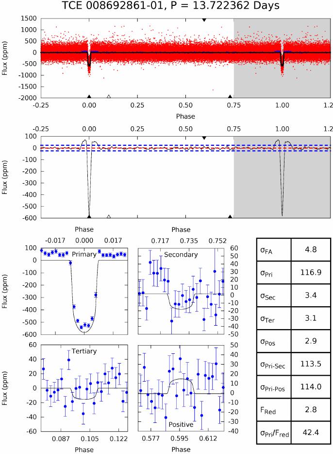
20 starting with Q represent the other quarters, up to Quarter 16 (Q16). The boxes labeled starting with Y are all data combined for the given year, where Year 1 (Y1) contains data from Q1-Q4, Y2 contains data from Q5-Q8, etc. The boxes labeled starting with S are all data combined for the given season, where Season 1 (S1) contains all data from Q1, Q5, Q9, and Q13, S2 contains all data from Q2, Q6, Q10, and Q14, etc. The box in the bottom-right labeled All contains all data for the target. Red points represent the raw data and blue points are binned data such that eight binned points will always be located in-transit. The black line, for all boxes, is the DV transit model fit to all of the data. While no tick marks are shown on the y axis for any box, since the model-fit shown by the black line is constant for all boxes, it provides a sense of scale. Model-Shift Uniqueness and Occultation Test Theory To search for additional events, we take the DV photometric time series folded at the orbital period of the primary event (see Figure 4) and use the DV-generated transit model as a template to measure the amplitudes of other transit-like events at all phases. The amplitudes are measured by effectively fitting the depth of the transit model centered on each of the data points. The deepest event aside from the primary transit event, and located at least two transit durations from the primary, is labeled as the secondary event. The next-deepest event located at least two transit durations away from the primary and secondary events is labeled as the tertiary event. Finally, the most positive flux event (i.e., shows a flux brightening) located at least three transit durations from the primary and secondary events is also labeled. We determine the uncertainty in the amplitude measurements by calculating the standard deviation of the photometric data points outside of the primary and secondary events. Dividing the amplitudes by this standard deviation yields significance values for the primary (σpri), secondary (σsec), tertiary (σter), and positive (σpos) events. Assuming there are P/Tdur independent statistical tests per TCE, where P is the period of the TCE, and Tdur is the transit duration, we can compute a detection threshold for each TCE such that this test yields no more than one false alarm when applied to all TCEs. We call this threshold σfa, and compute it via the following equation, σfa = sqrt(2)*inverfc[(tdur / P) (1/nTCEs)] where inverfc is the inverse complementary error function and ntces is the number of TCEs dispositioned. For the Q1-Q16 TCERT activity, we assumed a value of ntces = 10,000. Finally, we also measure the amount of systematic red noise in the lightcurve on the timescale of the transit by computing the standard deviation of the measured amplitudes outside of the primary and secondary events. We report the value FRed, which is this standard deviation of the measured amplitudes divided by the standard deviation of the photometric data points. FRed = 1 if there is no red noise in the lightcurve. It should be noted that if no DV fit was performed for the given TCE, this plot and its associated statistics cannot be generated, and does not exist. We show the full plot in Figure 13, present each individual panel in subsequent plots, and discuss how to use this plot and associated metrics for vetting. 20 of 32

21 21 of 32

22 Figure 13: Page 4 of the Kepler Q1-Q16 TCERT Vetting Products for each TCE. The top line shows the TCE ID and associated orbital period. The top panel shows the photometric observations from the DV detrended light curve (see Figure 3) phased to the orbital period of the candidate event. The middle panel shows the data fitted at other phases using the transit model. The bottom left panels show the primary event on the top left, potential secondary event on the top right, third strongest transit-like signal (tertiary) on the bottom-left, and the strongest transit-like signal with increasing flux (positive) on the bottom-right. The table on the right lists the values for the false alarm detection threshold (σfa), significance of the primary (σpri), secondary (σsec), tertiary (σter), and positive (σpos) events, the difference in significance between the primary and secondary events (σpri-σsec), the difference in significance between the primary and positive events (σpri-σpos), the ratio of the noise level on the timescale of the transit duration (red noise) divided by the Gaussian noise (Fred), and the significance of the primary event when taking into account the red noise (σpri/fred). Phased Lightcurve Similar to Figure 4, Figure 14 shows the Kepler DV photometric time-series phased to the orbital period of the primary event. The location of the primary event is marked by an upward, filled triangle at a phase of 0.0. The location of the best secondary eclipse candidate is marked by an upward, filled triangle at a phase other than 0.0. The location of the most significant tertiary event is marked by the location of the upward, open triangle. The location of the most significant positive flux event is marked by the location of the downward, filled triangle. Model Filtered Data Figure 15 shows the measured amplitude (or depth) at each phased, photometric measurement. The primary transit is always located at phase zero. A red dashed line is plotted at Flux = 0, with two blue dashed lines marking the fluxes that correspond to ±σfa. This figure is used to evaluate the significance of possible secondary events and, more generally, to help determine the uniqueness of the transit event. Primary, Secondary, Tertiary, and Positive Events We also present zoomed-in plots of binned photometry for the primary, secondary, tertiary, and positive events as shown in Figure 16. Only the binned data points, shown in blue, are shown for clarity, with the transit model at the best-fit depth shown via a black line. These can be very useful for establishing the credibility of σpri and σsec. We also note that the transit model is based on the whitened data, so mismatches due to flux differences before ingress and after egress are common. 22 of 32

23 Figure 14: The red points show the phased DV photometric light curve for the candidate event. Blue points show binned data, such that eight binned points lie within the primary transit. (In this example, as it is a high SNR planet candidate, the blue points mostly all lie behind the black model line.) The black line shows the best-fit transit model from DV. The primary event is located at phase zero and is marked by an upward-facing triangle on the bottom axis. The other triangles mark the locations of potential secondary (filled) and tertiary events (open); the location of the strongest anti-transit is marked by the downward-facing triangle on the top axis. The grayed out area from phase 0.75 to 1.25 plots the same data as is plotted between phases and Figure 15: The fitted amplitude of the transit at each phased, photometric measurement. A red dashed line is plotted at Flux = 0. The two blue dashed lines mark the fluxes that correspond to ±σfa, which is a Gaussian estimate of a detection threshold that will produce no more than 1 false-alarm for every 10,000 TCEs. The triangles mark the location of the primary, secondary, tertiary and anti-transit events as described for Figure 14. Note that the shoulders seen on either side of the primary event are due to the DV median detrending algorithm. 23 of 32

24 Figure 16: Phased and binned data zoomed in on the primary (top left), secondary (top right), tertiary (bottom left), and positive (bottom right) events. The line is an overlay of the best-fit transit model to each event. As the model fit is performed in the whitened domain, sometimes it will not match up perfectly with the flux-level data, as shown. Model-Shift Metrics We also report eight measurements on the right side of Page 4 (Figure 13): σfa,: The computed detection threshold for each TCE, above which we expect only one detection of a false alarm in 10,000 TCEs. Specifically, σfa = sqrt(2)*inverfc[(tdur / P) (1/nTCEs)], inverfc is the inverse complementary error function, Tdur is the transit duration, P is the period of the object, and ntces is the number of TCEs dispositioned. For the Q1-Q16 TCERT activity we set ntces = 10, of 32

25 σpri,: The significance of the primary transit. This value will appear in red if σpri < σfa. σsec: The significance of the next deepest event outside of the primary eclipse, which is labeled as a potential secondary. The phase of this event is constrained to not be within two transit durations of the phase of the primary. This value will appear in red if σsec > σfa. σter,: The significance of the third deepest event, aside from the primary and secondary. The phase of this event is constrained to not be within two transit durations of either the phases of the primary or secondary events. This value will appear in red if σter > σfa. σpos: The strongest positive or 'anti-transit' event. The phase of this event is constrained to not be within three transit durations of either the phases of the primary or secondary events, as the DV detrending can create positive shoulders on the edges of transits/eclipses. This value will appear red if σpos > σfa. σpri-sec: The significance difference between the primary and secondary events. This value will appear red if it is less than 3.0. σpri-pos: The significance difference between the primary and anti-transit events. This value will appear red if it is less than 3.0. FRed: The ratio of the level of red noise to the white, Gaussian noise. The level of red noise is computed by taking the standard deviation of the computed amplitudes at all phases outside of the primary and secondary events (see Figure 15), and dividing by the standard deviation of the photometric light curve outside of the primary and secondary events (see Figure 15). FRed = 1 if the noise spectrum is white. σpri / FRed: The significance of the primary transit when taking into account the amount of red noise in the lightcurve at the same timescale as the transit duration. This value will appear red if σpri / FRed < σfa. In general, if σpri/fred > σfa, we believe the transit candidate is real and not due to random noise or systematic fluctuations. If σpri-sec > 3 and σpri-pos > 3 then we believe the transit candidate is unique, i.e., it tells us there is a large difference between the transit event and other putative events in the rest of the phased photometric data. If σpri-sec < 3 or σpri-pos < 3 then the validity of the transit candidate is called into question because then there are other events in the light curve of comparable depth and signal-to-noise. The presence of an occultation is determined by σsec which is a measurement of the significance of the secondary event, analogous to σpri. Similar to the constraints on the primary, a secondary eclipse is generally considered detected if σsec/fred > σfa, σsec-ter > 3 and σsec-pos > 3. There is no outlier rejection performed in this analysis for the Q1-Q16 activity. Thus, one must be careful in interpreting these plots and results when very large outliers are present. The Model-Shift plots however will always show all points present, including outliers, while the DV plots (Figures 2-8) will not. Outlier rejection for the Model-Shift plots will be implemented for future TCERT activities. Page 5 Centroid Analysis Overview The centroid analysis pages provide more in-depth centroid information than what was presented in Figure 9 for the DV summary. Three different yet complementary reconstructions of the location of the transit signal relative to the target star are shown in Figure of 32

26 Figure 17: The Centroid Analysis Overview page, which is page 5 of the Kepler Q1-Q16 TCERT Vetting Products. The centroid offsets computed relative to the out-of-transit PRF fit, KIC position, and photometric centroids are shown from left to right. This page has three elements: 1. Descriptive information about the target: a) Kepler magnitude. This is important to identify saturated targets. When the target star is bright enough that saturation may be an issue this value is turned red. b) The transit SNR as measured by the DV transit model fit. This will generally indicate the quality of the difference images. c) The number of quarters with good difference images. This refers to the difference image quality metric, which tells you how well the fitted PRF is correlated with the difference image pixel data. A difference image fit is considered good if the correlation is > 0.7. If the correlation is smaller this does not mean that the quarter s difference image is useless, just that it must be examined carefully. When the number of good quarters is three or less this line is turned red. d) The distance from the out-of-transit PRF-fit centroid to the target star s catalog position. When this distance is > 2 arcsec this line is turned red. 26 of 32

27 2. A table giving the reconstructed location of the transit signal relative to the target star using three different but complimentary methods: a) The multi-quarter average offset of the PRF-fit difference image centroid from the PRF-fit out-of-transit (OOT) image. b) The multi-quarter average offset of the PRF-fit difference image centroid from the Kepler Input Catalog (KIC) position. c) The offset reconstructed from photometric centroids. For all of these methods the distance, significance, and RA and Dec components are reported. We consider an offset distance to be statistically significant when it is greater than 3 sigma and greater than ~0.1''. 3. Three panels showing the reconstructed location of the transit signal relative to the target star (located at 0,0), which correspond to the three rows of the table. The first two panels, based on PRF-fitting techniques, show the offset from the out-of-transit fit and the KIC position, respectively. In each of these the crosses represent each individual quarter, with the size of the crosses corresponding to their 1-sigma errors. The circle is the 3-sigma result for all quarters combined. The third panel shows the offset location based on photometric centroids, which provides only a multi-quarter result. As discussed previously, one should look to see if any bright stars are near the target that may influence the PRF fit by comparing the calculated offsets from the out-of-transit PRF fit and the KIC position. For more information on these metrics and the identification of false positives using the pixel-level data, see Bryson et al. (2013). Pages 6-9 The Pixel-Level Images The next four pages show the average difference and out-of-transit images for each quarter, which provide the data behind the PRF-fit centroids and the resulting multi-quarter average. These images are arranged so that they show four quarters, or a full year, per page. Each image shows three positions via markers: x marks the catalog location of the target star, + marks the PRF-fit centroid of the OOT image, and Δ marks the PRF-fit centroid of the difference image. The color bar is a crucial interpretation tool: when it is almost entirely positive for the difference image, this means that the difference image is reliable. When the color bar indicates negative values one should be more cautious. Large negative values are indicated with large, red X symbols, and may indicate that the difference images are unreliable, or that the TCE is due to systematics that do not have a stellar PRF. White asterisks indicate background stars with their Kepler ID and magnitudes. This includes stars from the UKIRT catalog, which have Kepler IDs > 15,000,000. These UKIRT Kepler IDs are internal project numbers and do not correspond with UKIRT catalog identifiers. A N/E direction indicator is provided to allow matching with the figures on page 5 (see Figure 17). 27 of 32

28 An example for quarters 1 and 2 is shown in Figure 18. The pixels highlighted by a red X in the difference image for quarter 1 represent pixel value variations that are slight increases in light during the transit, but since this quarter contains less data than others (~30 days in Q1 compared to ~90 days in other quarters) and is prone to detrending errors, they do not invalidate the difference image. When the high value pixels in the difference image are isolated and appear star-like we consider this to be a clear transit signal, such as is seen for quarter 2. When the location of those difference image pixels correspond with the location of the star s OOT image, we say that the transit signal s location is consistent with the target star location. In this TCE, for quarters 1 and 2 as shown in Figure 18, the difference images are consistent with the OOT images, and thus the transit signal originates from the target star. No centroid offset is observed. Page 10 The Multi-Quarter Pixel and UKIRT Images This page provides an average of the pixel-level images from all quarters, utilizing an alternate detrending technique. The pixel-level time-series flux data is detrended following the same procedure as described for the trapezoid-fit, alternate detrending plot (see Figure 11). The resulting detrended pixel time series is phase folded on the trapezoid model fit ephemeris, and the average relative flux change during transit is adopted as the transit depth for that pixel. The transit SNR for a pixel is calculated from the transit depth divided by an empirical estimate of the noise in the detrended out-oftransit pixel time series. The images are combined by choosing a reference quarter and aligning the other quarters' pixel-level images to it. The resulting SNR sky image is thus on the pixel grid of the reference quarter. Figure 19 shows the combined, multi-quarter SNR image in the top-left, the average depth in the bottom-left, the out-of-transit logarithmic flux in the bottom-right, and a UKIRT image of the area of the sky covered by the pixels in the top-right. On each image, the cyan square is the KIC position on the reference image. The cyan plus indicates the out-of-transit PRF fit location for the single quarter DV analysis. The magenta triangles indicate the difference image PRF fit location from each individual quarter. Since Figure 19 is an example of a high SNR planet candidate, all the symbols align on the target star, indicating that no significant centroid offset is seen. The purpose of the multi-quarter average is to turn quarter-to-quarter scatter into a statistical measurement of the most likely transit location. By combining the pixel-level images of all quarters, a higher SNR difference image can be obtained, which may reveal details not easily seen in the individual quarter difference images. In this case, as shown in Figure 19, the multi-quarter average and its uncertainty are strongly consistent with the location of the target star, so this TCE would be a centroid pass. When the high-value difference image pixels are isolated, star-like, and clearly different from the target star s out-of-transit image, then the multi-quarter average will indicate a statistically significant centroid offset, which indicates a centroid fail. Examining an alternate detrending also helps instill confidence that transit-like features haven't been artificially suppressed or enhanced by the DV detrending. Overlaying a UKIRT image on the observed pixels helps provide great utility for examining the stellar point sources at a higher resolution than provided by Kepler with its ~4 arcsecond pixels. 28 of 32

29 Figure 18: An example of the pixel-level images for Q1 and Q2 for Kepler-69b. The white x marks the catalog location of the target star, + marks the PRF-fit centroid of the out-of-transit image, and Δ marks the PRF-fit centroid of the difference image. Large red X symbols indicate significantly negative pixels. In this case of this PC, the out of transit flux image can be seen to match the difference image very well, indicating the observed transit signal originates from the target star. Page 11 Folded Flux and Flux-Weighted Centroid Time Series This page shows the flux-weighted photometric centroids, which can be used to determine if there is a centroid shift occurring at the time of transit. Unlike the difference images, this plot is guaranteed to exist for every TCE. In Figure 20, the top panel shows the phase-folded DV photometric time-series. The middle and bottom panels show the computed RA and Dec centroid offsets, respectively, for each photometric data point. A photometric offset can be considered to be observed if there is a change in the centroid time series (second and third panel) that looks like the flux time series (top panel). 29 of 32

30 Figure 19: An example of the multi-quarter, alternate detrending, centroid analysis. The photometric time-series of each individual pixel has been detrended utilizing the algorithm of Garcia et al. (2010). The bottom-right plot shows the average out-of-transit flux in a logarithmic scale for all quarters of data combined. The bottom-left plot shows the difference image (out-of-transit flux minus in-transit flux) for all quarters combined. The top-left image shows the difference image in units of signal-tonoise. The top-right image shows a registered UKIRT image with the same size as the pixel-level images. The + symbols mark the combined out-of-transit PRF fit location, the triangles mark the measured centroid of each quarter's difference image, and the square marks the target's KIC position. In the case of this TCE, most of the individual quarter centroid locations, target location, and out-oftransit centroid location stack on top of each other, thus showing no centroid offset. 30 of 32

31 Figure 20: The flux-weighted photometric centroids. Top: The DV phase-folded photometric time series. Middle: The computed RA centroid offset for each photometric data point. Bottom: The computed DEC centroid offset for each photometric data point. The purpose of this figure is to verify that if there is a measured photometric shift from the difference images, it looks like the transit signal, and thus isn't due to instrumental systematics. However, any amount of light in the aperture not from the target star will cause a centroid shift to appear in this plot, even when the signal does originate from the target star. Thus, this plot should never alone be used to centroid fail a TCE. Page 12 and Beyond If there are additional TCEs for the system beyond the first, they will show up as additional pages, replicating those described in Pages In each analysis, the in-transit data from previous TCE(s) will have been subtracted from the data. 31 of 32