Accurate Cosmology with Galaxy and Quasar Surveys. Boris Leistedt

Transcription

1 Accurate Cosmology with Galaxy and Quasar Surveys Boris Leistedt Submitted for the degree of Doctor of Philosophy Department of Physics and Astronomy University College London September 2014

2 I, Boris Leistedt, confirm that the work presented in this thesis is my own. Where information has been derived from other sources, I confirm that this has been indicated in the thesis. 1

3 Abstract Observations of the cosmic microwave background have led to a golden age of cosmology, where precise measurements can be confronted with predictions from cosmological models. Ongoing and future surveys of the distribution of galaxies will continue this revolution: they will enable us to test the laws of gravity, uncover the properties of dark energy and dark matter, and reinforce the connection to high-energy physics. However, current galaxy survey analyses are already limited by our ability to identify and treat observational systematics, and this problem will be even more pronounced in future experiments. Therefore, it is essential to develop novel methods to deal with these complications when testing cosmological models and searching for new physics. This is the focus of this thesis. Firstly, I will present measurements of primordial non-gaussianity obtained from the clustering of quasars from the Sloan Digital Sky Survey. Primordial non-gaussianity is a powerful probe of inflation, the leading theory of the initial conditions of the universe, but its effects on the distribution of quasars are mimicked by observational systematics. I will describe a framework to deal with these systematics and robustly measure primordial non-gaussianity from the clustering of quasars. Secondly, I will present a new set of wavelet transforms on the sphere and the ball. These approaches are highly promising for analysing cosmological and geophysical data and dealing with their systematics in novel ways. Finally, I will examine the recent claims that extra massive neutrinos can resolve the tensions between cosmic microwave background, galaxy survey and supernova observations. I will demonstrate that this conclusion is premature since it is driven by the least robust data sets. Given the growing number of cosmological observables and their varied levels of robustness, combining data sets and dealing with such tensions will become critical in the near future. 2

4 Acknowledgements First and foremost, I would like to express my deepest gratitude and appreciation to my advisor, Hiranya Peiris. During the past three years, you have been an attentive, supportive, and inspiring mentor, and I am extremely grateful for the infinite amount of time and energy you have invested in me. My time in UCL has been a life changing experience, and I could never hope for a better supervisor. I would also like to thank the exceptional individuals I have had the chance to collaborate with: Jason McEwen, Daniel Mortlock, Andrew Pontzen, Aurélien Benoit-Lévy, Licia Verde, Nina Roth, and Franz Elsner (in order of appearance). I have learned so much from you, both personally and scientifically, and you made me discover how fun, fascinating, and humanly enriching research could be. Thank you to Ofer Lahav and Filipe Adballa for the useful discussions and advice during the course of this PhD. I am also grateful to Alan Heavens and Benjamin Joachimi, who kindly accepted to examine this thesis and provide many useful comments and suggestions. My experience in UCL would not have been complete without the UCL astro-p(i)gs. For all the love, laughs and tears, I thank all the students and post-docs of the Astrophysics Group. Special thoughts go to the inhabitants of G16, this parallel universe where I worked during the three years of my PhD. Thanks to you I have enjoyed every single day in the office. I am indebted to my parents and my brothers for their unconditional backing over the years. Thank you for encouraging me and providing me everything I needed to follow my dreams. And finally, thank you Olivier, for standing by my side from the very first day, and making my life so colourful. Without your love and support, this document would simply be blank. 3

5 Contents 1 Introduction The Universe Composition and structure Brief history The early Universe The cosmic microwave background Inflation and primordial non-gaussianity The evolved Universe Matter perturbations and structure formation Galaxy surveys Scale-dependent halo and galaxy bias Quasars Cosmological neutrinos Wavelets in cosmology Thesis outline Estimating the large-scale angular power spectrum in the presence of systematics: a case study of Sloan Digital Sky Survey quasars Abstract Introduction Theory and methods Background

6 2.3.2 Partial sky coverage and quadratic estimators Likelihood analysis and band-powers Galaxy surveys, shot noise and systematics Illustration: recovering the power spectrum of the CMASS sample Application to SDSS photometric quasars Data and subsamples Theory predictions Redshift distributions estimates Masks and systematics Power spectrum results Discussion Aknowledgements Appendices Pixelisation, band-limit and smoothing issues Karhunen-Loève compression demystified χ 2 for band-power estimates Exploiting the full potential of photometric quasar surveys: optimal power spectra through blind mitigation of systematics Abstract Introduction Theory and methods Power spectrum estimation Extended mode projection Fast cross-power spectra and null-tests Application to SDSS photometric quasars Sample selection and redshift distributions Masks and systematic uncertainties Estimation settings and blind mitigation of systematics Power spectrum measurements Conclusion Acknowledgements

7 4 Constraints on primordial non-gaussianity from 800,000 photometric quasars Abstract Introduction PNG with photometric quasars XDQSOz power spectrum measurements Halo bias from PNG Monte Carlo Markov Chain (MCMC) analysis Results Future prospects Conclusion Acknowledgments S2LET: A code to perform fast wavelet analysis on the sphere Abstract Introduction Wavelets on the sphere Harmonic analysis on the sphere Scale-discretised wavelets on the sphere The S2LET code Multiresolution algorithm Implementation Numerical validation Future extensions Examples Wavelet transform from the command line Wavelet transform in Matlab and IDL Wavelet denoising in C Summary Acknowledgements Exact Wavelets on the Ball Abstract Introduction Harmonic Analysis on the Ball

8 6.3.1 The spherical Laguerre transform Relation to the spherical Bessel transform The spherical harmonic transform The Fourier-Laguerre transform Wavelets on the Ball Convolutions Exact flaglet transform Flaglets and scaling functions Multiresolution Algorithm Algorithm Fast implementation Numerical validation Denoising Illustration Wavelet denoising Examples Conclusions No new cosmological concordance with massive sterile neutrinos Abstract Introduction Data and methods No new concordance with sterile neutrinos Constraints on neutrino masses from robust datasets Conclusions Acknowledgments Bibliography 180 7

9 List of Figures 1.1 Current picture of cosmic history, as suggested by cosmological observations and explained by the concordance model The angular power spectra of the CMB temperature and polarization fluctuations measured by Planck (Planck Collaboration, 2013i) Example of an inflaton potential, from Baumann (2009) Power spectrum and bispectrum in Fourier space Matter power spectrum from a range of probes, reproduced from Hlozek et al. (2012), where the data sets are described in detail Left: measurements of the 3D power spectrum of galaxies from the Baryon Acoustic Oscillation Survey (Anderson et al., 2012). Right: tomographic angular power spectrum of luminous red galaxies from SDSS DR7 (Thomas et al., 2010) Kaiser effect and scale-dependent halo bias due to primordial non-gaussianity Typical spectral energy distribution of a quasar, from Vanden Berk et al. (2001) Effect of massive neutrinos on the matter and CMB power spectra, reproduced from Park et al. (2012) Example of mexican hat wavelets constructed to be localised in time and frequency domains (Couderc and Zareba, 1998). These wavelets are redundant, i.e., a given scale or frequency is probed by more than one wavelet Fiducial CMB and galaxy survey masks used to calculate the covariance matrices of Fig

10 2.2 Fiducial CMB and CMASS angular power spectra used to calculate the covariance matrices of Fig Covariance matrices V ll of the PCL and QML estimates calculated for the CMB and LSS spectra and masks in Figs. 2.1 and 2.2 in the absence of noise and systematics Mask of the CMASS DR9 sample in the Northern Galactic Cap Average PCL and QML estimates of the 600 CMASS mock catalogues Distributions of the photometric and spectroscopic redshift estimates of the RQCat UVX-LOWZ sample, cross-matched with the SDSS-DR7, BOSS and 2SLAQ spectroscopic quasar catalogues Histograms of the redshifts and apparent magnitudes of UVX-LOWZ objects in RQCat, and of objects with good spectra found in the SDSS-DR7, BOSS and 2SLAQ spectroscopic quasar catalogues Low-resolution redshift- and magnitude-dependent completeness corrections for estimating the redshift distributions of the RQCat subsamples through cross-matching with the SDSS-DR7, BOSS and 2SLAQ spectroscopic quasar catalogues Final estimates of the redshift distributions of the four RQCat photometric subsamples, calculated by cross-matching with the SDSS-DR7 spectroscopic quasar catalogue Theory predictions for the four RQCat subsamples computed with CAMB SOURCES Systematics templates used in this analysis, and the (dimensionless) angular power spectra C l of their overdensity maps Masks used for the power spectrum analysis of RQCat, in Equatorial coordinates Illustration of the suboptimality of the PCL estimator in the case of the Mid+High-z subsample QML estimates of the (dimensionless) auto-power spectra of the overdensity maps of the four RQCat samples presented in Fig QML estimates of the (dimensionless) cross-power spectra of the RQCat overdensity maps using the same conventions as Fig QML estimates for the (dimensionless) cross-power spectra of the four RQCat overdensity maps with the systematics templates using the same conventions as Fig Beams that apply to the power spectrum estimates of pixelised, smoothed maps at HEALPIX resolution N side Histograms of the χ 2 values of the PCL (left) and QML (right) estimates of the 600 CMASS mock catalogues

11 3.1 Redshift distributions of the photometric quasar samples selected with P QSO > 0.8 and top hat windows on the photometric redshift estimates ẑ p Templates of the main systematics selected as potential contaminants in the photometric quasar catalogues, and used within the extended mode projection approach A subset of systematics templates originating from the decorrelation (using Mask 1) of the basic set of systematics, a subset of which is presented in Fig Masks constructed for the power spectrum analysis of the XDQSOz samples Comparison of the reduced χ 2 obtained with the optimal and approximate QML cross-correlation estimators Distributions of the reduced χ 2 arising from null tests performed with the cross-power spectra of the four quasar samples with the 3700 orthogonal modes of the extended set of systematics templates Auto- and cross-angular power spectra of the four XDQSOz quasar samples measured with the quadratic maximum likelihood (QML) estimator Same as Fig. 3.7, but using extended mode projection Redshift distributions of the four quasar samples used in this analysis, parametrised as superpositions of normal distributions. The shaded regions show the 1, 2 and 3σ regions explored when adding 5% uncertainty to the parameters of these fits, which are included in the MCMC analysis Constraints on the quasar bias model described in Eq The solid line shows the fiducial model with b 0 = 1, β = 5, and the shaded bands show the 1σ constraints (b 0 = 0.96 ± 0.15, 68% CL, β and f NL marginalised) from the XDQSOz power spectra when varying the bias and PNG parameters, the shot noise, and the redshift distributions. The coloured bands show the results when fixing β = 5 and allowing a different bias amplitude in each redshift bin, to demonstrate the ability of the overall model to simultaneously describe the four samples Constraints on local-type f NL (in the ΛCDM+f NL model, with n fnl = g NL = 0) using the power spectrum analysis of XDQSOz quasars, for different bias models and incorporating uncertainties in the redshift distributions and cosmological parameters. The error bars show the 1 and 2σ constraints, the dashed line shows f NL = 0, and the shaded bands show the constraints from Planck (Planck Collaboration, 2013h)

12 4.4 1σ and 2σ joint constraints on f NL and g NL for the (b 0, β) + n(z)+cosmo case, i.e., marginalising over the uncertainties in the cosmological parameters, redshift distributions, and bias model σ and 2σ joint constraints on f NL and n fnl for the extended model of Eq. 4.3, marginalising over the same parameters as Fig Wavelets and scaling function constructed with the scale-discretised (SD), needlet and B-spline generating functions with parameters λ = 3 and J 0 = 2 and for band-limit L = Wavelets for scales j {2, 3, 4, 5} and scaling function constructed through a tiling of the harmonic line using scale-discretised functions Scale-discretised wavelet transform of a band-limited topography map of the Earth for λ = 3, J 0 = 2 and L = 128, i.e. with the scale-discretised wavelets shown in Figure Numerical accuracy and computation time of the scale-discretised wavelet transform computed with S2LET Wavelet denoising by hard-thresholding, using parameters λ = 2 and J 0 = 0 and scale-discretised generating functions Spherical Laguerre sampling scheme on r [0, 1] for increasing band-limit First six spherical Laguerre basis functions K p (r) constructed on r [0, 1] and the associated sample positions Slices of an axisymmetric flaglet wavelet kernel constructed on the ball of radius R = 1, translated along the radial half-line Tiling of Fourier-Laguerre space at resolution L = N = 64 for flaglet parameters λ = ν = 2, giving J = J = Slices of four successive axisymmetric flaglet wavelet kernels, probing different scales in angular and radial space Numerical accuracy and computation time of the Fourier-Laguerre transform computed with FLAG Numerical accuracy and computation time of the flaglet transform computed with FLAGLET Flaglet decomposition of the N-body simulation dataset considered for the first denoising example

13 6.9 Denoising of an N-body simulation Denoising of a seismological Earth model Constraints on the ΛCDM+N eff + m eff ν,sterile model, showing that non-zero sterile neutrino mass is only favoured as a result of a tension between the CMB and cluster data (PlaSZ, Xray) in the σ 8 Ω m plane, and the degeneracy between σ 8 and neutrino mass Persistence of the tension as the minimal ΛCDM model is extended in the neutrino sector, i.e., as N eff and massive active or sterile neutrinos are added Constraints on the ΛCDM+ r N eff + m eff ν,sterile model, illustrating the persisting tension between X-ray clusters and CMB+BAO in the σ 8 Ω m plane, despite an apparent reconciliation of the BICEP and Planck results on r

14 List of Tables 2.1 Number of objects in the four RQCat redshift subsamples, and for which good spectra (and thus good spectroscopic redshifts) were found in the SDSS-DR7 quasar catalogue Systematics thresholds used to restrict the power spectrum analysis of RQCat to the most reliable regions of the sky to minimise contamination from calibration errors The chi square values for the auto- and cross-power spectra of the four RQCat samples presented in Figs and 2.15, with and without mode projection (mp) The chi square values for the cross-power spectra of the four RQCat samples with the systematics templates, presented in Fig. 2.16, using the same conventions as Table The chi-square values for the power spectra measured using extended mode projection with Mask 2, presented in Fig PNG constraints for different models. The base model is (b 0, β)+cosmo+n(z). The first super/subscript corresponds to the 68% CL, and the 95% CL can be obtained by adding the second number Order of magnitude of the accuracy of the HEALPix spherical harmonic transform Evidence ratios between the minimal ΛCDM model and the extended neutrino models Marginalised 95% CL constraints on the ΛCDM+N eff + m ν model from a variety of robust LSS datasets with the Planck CMB temperature and lensing measurements Same as Table 7.2, but for the ΛCDM+N eff + m eff ν,sterile model, showing tight constraints on the mass of sterile neutrinos

15 7.4 Evidence ratios ln[e ΛCDM /E ext. ] between the minimal ΛCDM model and the ΛCDM+ r N eff + m eff ν,sterile model, showing that sterile neutrinos are not favoured by the data, even when adding the BICEP results

16 1 Introduction The purpose of models is not to fit the data but to sharpen the questions.. S. Karlin 1.1. The Universe Cosmology is the quantitative study of the Universe as a whole: its content, origin, evolution, and fate. Its recent success as a precision science mostly rests on two pillars: large data sets mapping the Universe on a wide range of scales and frequencies, and a remarkable model describing these observations at unprecedented fidelity. Yet, many questions remain unsolved, and cosmology is an active field of research, requiring a vital balance of theory and observation, and overlapping with numerous other disciplines including astronomy, chemistry, particle physics, statistics, signal processing, and machine learning Composition and structure The fundamental assumption of the current concordance model ΛCDM, summarised in the following sections is the homogeneity and isotropy of the Universe on large scales. Supported by a range of observations, this idea has been promoted to a guiding axiom: the Cosmological Principle, stating the Universe looks the same for all observers, whoever and wherever they are. A natural consequence of this axiom is the assumption that the observable Universe is a fair sample, i.e., representative of the whole Universe, and that the same physical laws apply throughout. Violations of these assumptions are under investigation, but they are not considered in this thesis. 15

17 One of the pillars of the ΛCDM model is the theory of General Relativity (GR), which describes the interplay between mass, gravity, and space time. A good review GR from a cosmological perspective is provided in Dodelson (2003), and we use the same conventions here. Following the principles of GR, the Universe can be viewed as an evolving object, the structure and dynamics of which are influenced by its content, and vice versa. More precisely, in the current concordance model, the Universe is mainly composed of four ingredients: Baryonic matter: visible matter interacting through gravitational, electromagnetic, strong and weak forces, composing stars, planets, and living organisms. Making up only 4.9% of the total energy budget today, it mostly contains hydrogen and light elements formed in the early Universe. Relativistic species: electromagnetic radiation and neutrinos, mainly produced in the early Universe in the form of the cosmic microwave and neutrino backgrounds (CMB and CνB, respectively). They are currently subdominant in energy density compared to the other components, but played an essential role in earlier epochs (see details below). Cold dark matter (CDM): non-baryonic, pressureless, non-relativistic matter, that interacts very weakly (or not at all) through the electromagnetic force. Although it hasn t been directly observed or produced, its existence is well motivated by a range of observations including the CMB, galaxy rotation curves, galaxy clustering (Davis et al., 1982; Oort, 1932; Rubin and Ford, 1970; Zwicky, 1933) and gravitational lensing of galaxies and clusters (Clowe et al., 2004, 2006; Dietrich et al., 2012; Massey et al., 2007; Taylor et al., 1998). It makes up 26.8% of the energy budget of the Universe, and played a crucial role in the formation of structures in the Universe, such as galaxies and clusters of galaxies. CDM remains by far the simplest and most successful joint explanation of a plethora of phenomena. The detection of its associated particles as well as understanding baryonic physics in the CDM context (e.g., in galaxy formation) are active fields of research (see e.g., Aalseth et al. 2011a,b; Angle et al. 2008; Bernabei et al. 2008). Dark energy (Λ): it dominates the energy budget of the Universe today (68.3%) and drives a phase of accelerated expansion (Perlmutter et al., 1999; Riess et al., 1998, 2004). It is currently indistinguishable from a cosmological constant, which poses a deep theoretical challenge. In particular, when considered as vacuum energy, the theoretical prediction under estimates the observed value by 120 orders of magnitude. This discrepancy is likely due to our 16

18 inability to unify quantum physics and GR and correctly compute all the contributions to the energy of the vacuum. Modern reviews of these theoretical challenges can be found in Carroll (2001), Clifton et al. (2012), and Martin (2012). Dark energy is a pressing question, and the search for deviations from a cosmological constant are high priorities of modern observational cosmology. Cosmological observables such as the CMB and galaxy surveys, detailed in subsequent sections, inform us about the proportions of these four constituents, which have dominated the energy budget in various epochs, and influenced the formation of structure and the expansion history of the Universe. The idea of an expanding Universe was introduced to resolve the apparent violation of homogeneity in Hubble s observations of the recession of galaxies. The expansion is encoded in the scale factor a, which is isotropic and a function of physical time t only, with a = 1 today. The space-time metric g µν of the expanding, homogenous, isotropic Universe takes a simple form, ( ) dr g µν dx µ dx ν = c 2 dt 2 + a 2 2 (t) 1 kr 2 + r2 (dθ 2 + sin 2 dφ 2 ). (1.1) In this metric, often called the Friedmann-Lemaitre-Robertson-Walker (FLRW) metric, (r, θ, φ) are the 3D polar coordinates labelling the points of the 3-dimensional constant-time slice, thereby defining comoving observers. k is a measure of the spatial curvature, reduced to canonical values k = +1, 0, 1 corresponding to a constant-positive-curvature, a flat, and a negative-curvature 3D spaces, respectively. Another important quantity is the conformal time η, η dt a(t), (1.2) which is used to defined the comoving particle horizon in the time interval t t i, denoted by χ(t) = η η i. The latter is the maximum comoving distance travelled by a photon traveled between t i and t, and therefore defines a causal horizon beyond which particles have not been causally connected since t i. In addition, solving for the geodesics equations g µν dx µ dx ν yields that the physical momentum and energy of photons scale as a 1 as the Universe expands, the result leading to the definition of redshift z, λ obs λ em 1 + z = a(t obs) a(t em ), (1.3) connecting the wavelengths and scale factors at emission and observation times (t em and t obs, respectively). For observations made today, we have t obs = today and a(t obs ) = 1 by convention. 17

19 For small redshifts, expansion around t obs yields the famous Hubble law cz H 0 d with the Hubble constant defined as H 0 = 1 da a dt, (1.4) tobs sometimes expressed in terms of the dimensionless parameter h as H 0 = 100 hkms 1 Mpc 1. While early measurements of cepheids yielded h 0.7 (Sandage, 1958), current CMB, supernovae and gravitational lensing measurements are able to pin down H 0 to percent level. However, some of the most recent measurements are discrepant (Freedman et al., 2001; Hinshaw et al., 2013; Planck Collaboration, 2013k; Riess et al., 2011a), and it is unclear whether this points to new physics or to residual systematic uncertainties in the measurements. Extra relativistic species in the early universe, such as neutrinos, could alleviate these tensions if they are confirmed. This issue is briefly considered below and in the last chapter of this thesis. Assuming GR as a theory of gravity, the dynamics of the Universe are beautifully encapsulated in terms of the Friedmann and Lemaître solution of the Einstein equations, (ȧ ) 2 = a ä a 8πGρ 3 k a 2 + Λ 3 (1.5) = 4πG 3 (3P + ρ) + Λ 3. (1.6) These equations often called the Friedmann equations connect the content and the (background) expansion of the Universe, entirely captured in the time-dependent scale factor a(t). The components are encoded in the equation of state P = P (ρ), which can be written as P = wρ for perfect fluids. Relativistic particles have w = 1/3, matter w = 0, and cosmological constant w = 1, although the search for deviations from w = 1 is an active research topic. Using the equation of state a byproduct of the Einstein and Friedmann equations, ρ + 3ȧ (ρ + P ) = 0, (1.7) a one finds the solution ρ(a) = ρ 0 a 3(1+w). This result, in conjunction with the Friedmann equations, gives t 2/3(1+w), w 1 a(t) = e Ht, w = 1. (1.8) for a flat universe. In other words, a radiation-dominated Universe has a t, whereas matterdomination yields a t 2/3. A cosmological constant drives an exponential solution (with a constant 18

20 Hubble parameter H = H). Finally, the Friedmann equations can be rewritten in terms of the critical density ρ cr = 3H 2 /8πG, to pull out an explicit curvature term Ω(a) 1 = k H 2 a 2, (1.9) where Ω(a) is the total energy density in units, Ω(a) = ρ/ρ cr. Observationally, the Universe appears to be spatially flat (i.e., Ω = 1), but this raises an important fine-tuning problem the flatness problem, for the initial conditions of the cosmological model, as detailed below Brief history The observable Universe was smaller, denser and hotter in the past. In the standard cosmological paradigm, described in the next section, an initial phase of inflation is assumed to have caused a 60 e-fold (=e ) accelerated expansion and imprinted a distinctive, nearly scale-invariant spectrum of perturbations on a smooth background. Inflation is discussed in more details below. After this initial phase, the Universe was filled with an ionised baryon-electron-photon plasma. The mean free path of photons subject to Thomson scattering was extremely short due to the high number density of free electrons. During this radiation-dominated epoch, the Universe expanded as a t and cooled, steadily decreasing the mean photon energy, and eventually becoming dominated by matter rather than radiation. Recombination occurred at a temperature of about 3000 K, when the Universe was about 380,000 years old. Electrons and protons of the primordial plasma combined into neutral atoms, while photons began to free-stream, their mean free path becoming larger than the Hubble scale. This is when the CMB was emitted. The Universe then remained matter dominated for a long period, expanding as a t 2/3, and allowing matter perturbations to grow as the scale factor. Cosmic structures started to form: stars, quasars, galaxies, clusters of galaxies. The period between recombination and the formation of light sources is known as the dark ages. Reionisation occurred when the first objects were energetic enough to ionise neutral hydrogen, slowly filling the Universe with an ionised plasma. This process is believed to have occurred between 150 million and one billion years after inflation. These estimates will soon be refined by precise observations of the polarisation of the CMB, and by 21-cm experiments, which will map the neutral hydrogen in the epoch of reionisation. At the age of 10 billion years, the 19

21 Today : dark energy domination Galaxy formation 400 million years : End of reionisation Dark ages 380,000 years : cosmic microwave background Universe fully ionised Inflation and reheating Figure 1.1: Our picture of cosmic history, as suggested by cosmological observations and explained by the concordance model. Universe started to undergo a new period of accelerated expansion, presumably driven by dark energy, which stopped the growth of matter perturbations on all scales. Figure 1.1 gives a cartoon overview of the various stages of the history of the Universe, starting from a phase of inflation to the recent dark energy domination epoch. If the accelerated expansion persists, it will prevent any more structures from entering the cosmological horizon, and new gravitationally bound structures from forming The early Universe The cosmic microwave background As previously discussed, recombination of electrons and protons occurred when the Universe cooled below 3000 K, leading to the emission of relic radiation known as the cosmic microwave background (CMB). The CMB is the cornerstone of modern cosmology and one of the pillars of the ΛCDM model. First detected by Penzias and Wilson (1965), then identified by Dicke et al. (1965), its spectrum is the most perfect black body spectrum ever measured. It was first measured by COBE (Smoot et al., 1992), which also detected its temperature fluctuations of the order of 1 in 20

22 100,000 which have since then been studied by a great number of experiments. In particular, the WMAP satellite mission (Spergel et al., 2003) revealed the extraordinary informative power of these fluctuations, and firmly established cosmology as a precision science. More recently, the Planck satellite (Planck Collaboration, 2013g) refined our understanding of these fluctuations. Planck also bridged the gap between WMAP, mapping 0.2 degree scales, and experiments like the South Pole Telescope (Keisler et al., 2011) and the Atacama Cosmology Telescope (Dunkley et al., 2011), which focused on very small ( 0.1 deg 2 ) angular scales. The angular power spectra of the temperature and polarisation fluctuations from the first Planck release are shown in Figure 1.2. Their amplitude and features are intimately related to the composition and physical laws of the early Universe. For instance, the peaks of the power spectra constrain the curvature, the amount of dark matter and dark energy, whereas the damping tail informs us about the number of relativistic species at the time of recombination. Figure 1.2: The angular power spectra of the CMB temperature and polarization fluctuations measured by Planck (Planck Collaboration, 2013i). Not only is the physics of the CMB itself well understood and tested, but CMB experiments also provide a number of secondary observables. In particular, the lensing of the CMB by the intervening matter can now be mapped at great accuracy (Das et al., 2011; Planck Collaboration, 2013d; van Engelen et al., 2012), and is becoming established as a powerful cosmological probe. Finally, the CMB temperature maps can be used to search for physics that is not captured by angular power spectra. Indeed, the latter only contain all the information if the CMB is Gaussian. This has been tested to excellent precision, but current measurements leaves room for small 21

23 deviations, which will be discussed in the next section. Beyond (non-)gaussianity of the CMB, mapbased techniques are used to search for specific physics or features in the CMB, such as signatures of collisions with bubble Universes, cosmic strings, and deviations from homogeneity or isotropy. These are beyond the scope of this thesis, but some of the most recent investigations can be found in Feeney et al. (2013); Planck Collaboration (2013a,b,c) and references therein Inflation and primordial non-gaussianity The CMB offers a unique picture of the early Universe, and Figure 1.2 shows that it is remarkably well described by the ΛCDM model. However, a number of phenomena are unexplained without appropriate initial conditions, set by an initial phase of inflation. A pedagogic review of these problems and how to resolve them is presented in Baumann (2009). Here I only summarise how the inflationary paradigm addresses the horizon and flatness problems. The horizon problem results from the observation that the CMB is uniform to 10 5, and that this uniformity cannot be explained by causality alone. Indeed, in ΛCDM Fourier modes can only evolve from outside to inside the horizon, since the radiation- and then matter-dominated Universe has been in decelerating expansion from recombination until recent times, before dark energy started to dominate. In fact, the particle horizon in the ΛCDM model is approximately 1 degree on across the CMB sky, which is at odds with the measured full-sky uniformity. The flatness problem results from analysing Equation 1.9 and noticing that spatial flatness is an unstable point; in other words any deviation from flatness grows with time. Since CMB observations indicate that the Universe is spatially flat to percent level (i.e., the total density today is close to the critical density), it must have been even flatter in the past. One can extrapolate these constraints to find e.g., Ω 1 < O(10 16 ) at the time of nucleosynthesis, yielding a striking fine-tuning problem. Inflation is an elegant solution to these problems, and is currently the leading theory for the initial conditions of the Universe. It consists of a period of quasi-de Sitter expansion with H 2 Ḣ, where comoving separations grow as a(t) = e Ht and can cross the horizon. But one of the features of inflation is that it must end, i.e., it must only last for a finite period, and then return to a standard picture of matter and radiation domination. Therefore, a cosmological constant alone is not a viable solution since it would give constant H. This corresponds to the old inflation scenario (Guth, 1981; Guth and Weinberg, 1981): a scalar field trapped in a false vacuum. Therefore, a viable model of inflation requires a physical clock (Linde, 1982). One simple implementation of 22

24 this idea is a rolling scalar field with Lagrangian L = 1 2 µφ µ φ V (φ). The potential energy produces an exponential expansion rate, solving both the horizon and flatness problems provided the scale factor increases by at least a factor of e 60. The condition H 2 Ḣ therefore translates into V (φ) φ 2, and inflation ends when reaching the bottom of the potential, to undergo oscillations and reheat the Universe. This process is illustrated in Figure 1.3. This reheating converts the potential energy of the inflaton into particles of the Standard Model. (see e.g., Allahverdi et al for a review). Quantum density and metric fluctuations are generated during inflation, yielding powerful predictions, such as the near scale-invariance of its scalar perturbations and the existence of tensor perturbations producing gravitational waves. The latter leave a distinctive large-scale angular power in the B-mode polarisation of the CMB, the detection of which is one of the main goals of ongoing CMB experiments. Figure 1.3: Example of an inflaton potential, from Baumann (2009). CMB fluctuations are created by quantum fluctuations δφ, and acceleration occurs when the potential energy of the field dominates over its kinetic energy. Inflation ends at φ end when the kinetic energy has grown to become comparable to the potential energy. At reheating, the energy density of the inflaton is converted into radiation. Inflation is a successful phenomenological model, but its exact physical implementation is currently poorly understood. Dozens of classes of models exist, with hundreds of different variants, all solving the previous horizon and flatness problems (see Planck Collaboration et al for a set of models tested with Planck data). In addition, there is currently a growing ambition to implement inflation in the context of a more fundamental theory, such as string theory. Therefore, pinning down the detailed physics of inflation and reducing the space of models with observational constraints is a pressing question. 23

25 One of the most important observables that can help discriminate between classes of inflationary models is primordial non-gaussianity (PNG), denoting deviation from Gaussianity in the primordial fluctuations. In the CMB, since angular power spectra only measure the Gaussian information, PNG is measured by higher-order correlations, such as bispectra and trispectra, i.e., correlations between triplets and quadruplets of modes on the sky, as illustrated in Figure 1.4. k 1 k 2 k 1 k 2 P (k 1, k 2 ) = P ( k 1 k 2 ) k 1 k 2 k 3 k 2 /k 1 squeezed equilateral folded B(k 1, k 2, k 3 ) = B( k 3 k 1, k 2 k 1 ) k 3 /k 1 Figure 1.4: Power spectrum and bispectrum in Fourier space. Conditions P ( k 1 k 2 ) and B(k 1, k 2, k 3 ) = B( k3 k 1, k2 k 1 ) ensure that they are equivalent to the 2- and 3-point correlations in real space. The power spectrum is a one-dimensional curve; the bispectrum is a two-dimensional surface which is a function of the triangle formed by (k 1, k 2, k 3 ). In the context of inflation, limiting configurations (squeezed, equilateral, folded) correspond to different physical mechanisms. Specific physical mechanisms during inflation will create correlations in different configurations and shapes. For this reason, PNG is a powerful window on inflation. In particular, canonical singlefield slow-roll inflation predicts negligible level of squeezed-type PNG (see e.g., Allen et al. 1987; Bartolo et al. 2004; Maldacena 2003; Salopek and Bond 1990). Any measurement of deviations from this prediction can thus provide evidence for non-standard inflationary physics. This specific form of PNG arising from squeezed configurations is the so-called local model, where the primordial potential φ is modified by including higher order terms, Φ = φ + f NL [φ 2 φ 2 ] + g NL [φ 3 3φ φ 2 ], (1.10) where all fields are evaluated at the same spatial coordinate, and f NL and g NL are real-valued 24

26 constants (often called the skewness and kurtosis parameters). The most stringent constraints on local PNG currently come from higher-order statistics of the CMB. Most recently, the Planck Collaboration reported 8.9 < f NL < 14.3 (95% CL) (Planck Collaboration, 2013h), while constraints on the kurtosis have been obtained from the WMAP satellite, also consistent with g NL = 0. While these results are compatible with Gaussian initial conditions, their uncertainties still leave room for non-standard inflation models. Importantly, PNG can be detected in surveys of the large-scale distribution of galaxies, as detailed below. Performing this measurement in real data is one of the objectives of this thesis The evolved Universe The CMB is a powerful window on the early Universe, but is not sensitive to all predictions of the ΛCDM model. For example, the effects the dark energy are only detectable on the largest angular scales through the Integrated Sachs-Wolfe (ISW) effect, the blueshifting of CMB photons due to evolving potential wells at late times. Relativistic species like neutrinos are hard to distinguish from radiation, and theories of gravity can only be tested indirectly through their geometrical effects. Finally, the CMB is a surface by nature, and CMB temperature experiments like Planck are already on the verge of being limited by the number of modes ( 10 6 modes). Even though CMB polarisation and lensing have not yet reached their full maturation, they will also be ultimately limited by the statistical power of the last scattering surface. On the contrary, the large-scale structure of the Universe is a three-dimensional structure giving access to a much larger number of modes, and a plethora of additional observables. Ongoing and future experiments like the Dark Energy Survey 1 (DES), Euclid 2, the Square Kilometer Array 3 (SKA), the Large Synoptic Survey Telescope 4 (LSST), will probe > 10 9 modes and an immense range of physical processes, scales and epochs, which will allow us to test detailed scale- and redshift-dependent models of dark matter, dark energy, gravity, and baryonic physics

27 Matter perturbations and structure formation Figure 1.5 shows the power spectrum of the matter perturbations today (z = 0), i.e., fluctuations in the dark matter and baryon fluid, superimposed with a variety of observables. This again highlights the remarkable success of the ΛCDM model to describe cosmological observations in a range of scales and frequencies. The form of the matter power spectrum can be derived with linear perturbation theory and evolving the primordial scale-invariance power spectrum P (k) k, as summarised below. Figure 1.5: Matter power spectrum from a range of probes, reproduced from Hlozek et al. (2012), where the data sets are described in detail. The turnover scale around k 0.02 hmpc 1 is due to the very different physics that affects the modes entering the horizon before or after matter-radiation equality. The largest scale modes are always bigger than the horizon ( super-horizon ) and don t evolve through causal processes. During radiation- and matter-dominated epochs, they grow linearly with conformal time, and become constant once dark energy starts to dominate. At intermediate scales, modes enter the horizon after matter-radiation equality and evolve in a dark matter-dominated Universe. Since cold dark matter is pressureless, in this case the perturbations also grow linearly with conformal time. The smallest-scale modes, however, enter the horizon before matter-radiation equality and evolve in a radiation-dominated Universe. Therefore, the power at these scales is suppressed by a factor of 26

28 k 4 due to oscillations in the photon plasma, yielding the k 3 scaling of the matter power spectrum at k > 0.1 hmpc 1. The matter power spectrum is a rich source of cosmological information, since it is sensitive to the composition, initial conditions, and evolution of the Universe Galaxy surveys Unlike the CMB, the distribution of matter is not directly observable. It is sampled by tracers of the light distribution, such as galaxies and quasars, which probe the large-scale structure through their positions, and the magnification and lensing of their light by gravity. This thesis focuses on the study of the clustering of galaxies and quasars found by wide area surveys. Obviously, other tracers can be used, such as the distribution of neutral hydrogen, measured in the Lyα forest of quasar spectra or with future 21cm radio surveys. Their study can bring a great deal of information about baryonic physics and the z > 1 Universe. There are two distinct types of surveys of the large-scale structure (with a spectrum of intermediate cases, not considered here): spectroscopic and photometric surveys. In the former, one uses a high-resolution spectrograph to stare at bright sources and acquire their spectral energy distribution to estimate their type, characteristics and redshift. Hence, such surveys provide the 3D positions of galaxies and quasars, and can be used to map the large-scale structure in great detail. However, they are limited by the sensitivity of the spectrographs, and by the time and financial constraints needed to acquire good spectra of large numbers of sources. Photometric surveys, on the contrary, make use of broad band filters and wide-field cameras to overcome these constraints. They can detect faint sources (typically hundreds of millions of galaxies) over large areas of the sky (from hundreds to tens of thousands of square degrees), giving access to larger volumes and higher statistical power. Obviously, other complications arise, since the light spectrum is now only observed through a handful of filters. Topical issues include detecting sources and classifying sources (e.g., distinguishing galaxies from stars), estimating their fluxes and shapes in noisy images, and estimating their photometric redshift (photo-z). Most of these issues remain open problems and intense areas of research. Interestingly, some of them benefit from machine learning techniques (e.g., Collister and Lahav 2004; Graff et al. 2014), such as neural networks, which efficiently find classification and estimation rules in existing data and prove useful when physical models are not available or perform poorly (e.g., for photo-z estimation and star-galaxy separation). 27

29 Photometric surveys also rely different types of analysis compared to spectroscopic surveys. In general, photo-z estimates contain significant uncertainties, causing the radial distribution of detected galaxies to be poorly known. Hence one cannot probe the 3D distribution of matter, for example through 3D statistics such as the Fourier power spectrum P (k). The most common alternative is to measure the projected clustering of galaxies, involving 2D statistics such as angular power spectra or 2D correlation functions, in redshift slices of size greater than the photometric redshift uncertainties. In the best cases (with good photo-z), using sufficiently small bins and crosscorrelations between overlapping redshift samples enable the recovery of most of the information compared to the 3D distribution. Some of the most recent measurements of the 3D and 2D clustering of galaxies are presented in Figure 1.6. A notable advantage of exploiting angular power spectra in redshift bins is to keep the angular and radial dimensions decoupled in the analysis. This can facilitate the treatment of redshift dependent effects (sometimes difficult to incorporate in P (k) approaches 5 ), and observational complications or systematics, which usually affect the angular and radial information differently. The identification and robust treatment of systematics is a central point of this thesis. Indeed, future surveys will not be limited by statistical uncertainties, but rather by our ability to deal with systematics. The balance between depth, volume, photo-z uncertainties, and systematics can advantage spectroscopic and photometric surveys in different applications. The former are currently used for accurate measurements of the 3D power spectrum and bispectrum, mainly aiming at sub-percent level measurements of baryon acoustic oscillation feature. But the largest ongoing and future surveys the Kilo Degree Survey 6 (KiDS), DES, Euclid, LSST are all photometric. Beyond the gain in volume and statistical power, this is also because such surveys are optimal for measuring and combining information from the clustering and gravitational lensing of galaxies. These quantities do not only probe different scales and types of physics, but also suffer from different systematics. In particular, cosmic shear the magnification of light and distortion of shapes of galaxies due to gravity is a powerful window on the matter distribution, but also involves complications such as intrinsic alignment and shape measurement noise. The agreement but also complementarity between various probes of the large-scale structure is illustrated in Figure 1.5. The ΛCDM model remarkably fits all datasets, but future experiments will decrease the errors on these measurements by orders of magnitude. Combining data sets and testing models will then be challenging. 5 Most spectroscopic P (k) analyses assume no redshift evolution within the redshift range of the sample. It can be shown that sample spanning a large redshift range requires the a full 3D approach, for example involving the Fourier-Bessel transform, to exploit all the information

30 Figure 1.6: Left: measurements of the 3D power spectrum of galaxies from the Baryon Acoustic Oscillation Survey (Anderson et al., 2012). Right: tomographic angular power spectrum of luminous red galaxies from SDSS DR7 (Thomas et al., 2010) Scale-dependent halo and galaxy bias Connecting the distribution of light tracers to the underlying matter is a difficult task, due our limited knowledge of the physics controlling the formation and evolution of galaxies in dark matter halos. These complications are usually encapsulated in a galaxy (or quasar) bias term, which is added on top of the halo bias, to relate the galaxy and the dark matter overdensity fields. In its simplest incarnations well verified observationally for certain types of galaxies the bias is linear and scale-independent on large-scales, and becomes non-linear, and scale-dependent on small scales. The development of bias models is an active field of research, involving theoretical investigations and extensive comparisons to cosmological simulations. A major challenge of ongoing and future surveys will be to connect phenomenological bias models (fitted to measurements of the clustering of galaxies as a function of scale, luminosity, galaxy type) to the underlying physics of dark matter halo and galaxy formation. Interestingly, the halo bias itself can be affected by primordial physics. The example considered in this thesis is primordial non-gaussianity, which couples large and small scale modes in the initial conditions. This coupling can propagate and modify the abundance of halos in overdense regions (by tilting the halo mass function), therefore also affecting the number of galaxies in a scale-dependent manner. The effect can be visualised in Figure 1.7: non-zero local PNG will 29

31 δ c δ(x) Figure 1.7: The Kaiser effect (Kaiser 1984) describes the fact that galaxies form at the peaks of the primordial density fluctuations. Squeezed non-gaussianity increases the large scale modulation of the density peaks and thus impacts the clustering of tracers. Compared to the Gaussian case, not only are tracers more massive but they are more correlated over large distances, which modifies the bias of the power spectrum at large-scales. increase the abundance of massive halos on either large or small scales (for positive and negative f NL, respectively). Therefore, the net signature of primordial non-gaussianity on the large-scale structure is an enhancement of the bias of tracers on large-scales. Quantitatively, non-zero f NL and g NL will modify the Gaussian bias b G (z) into (Dalal et al., 2008; Desjacques and Seljak, 2010b; Matarrese and Verde, 2008; Slosar et al., 2008; Smith et al., 2012) b NG (k, z) = b G (z) + β f (z)f NL + β g (z)g NL α(k, z) (1.11) β f = 2δ c ( b G (z) 1 ) (1.12) β g = 3 log n f NL (1.13) α(k, z) = 2k2 T (k)d(z) 3Ω m H 2 0 (1.14) where δ c is the spherical collapse threshold, n the halo number density, and α(k, z) relates the linear density field and the primordial potential through δ lin (k, z) = α(k, z)φ(k). These expressions neglect an additional small contribution induced by the effect of PNG on the halo mass function (which can absorbed in b G ). For simplicity, the implicit mass dependence of b G, β f, and β g is also neglected, and the bias b G is considered to be only redshift dependent. Note that for β g we use the fitting formula from Smith et al. (2012), which is valid for the range of masses and scales considered in this thesis. Primordial non-gaussianity is powerful window on the early Universe, and it is remarkable that 30

32 its effect can be measured in the bias of large-scale structure tracers. However, measurements of the bias on large scales are largely limited by cosmic variance and the presence of spurious large-scale correlations, often produced by contamination from observational systematics. This thesis deals with this specific problem, i.e., measuring the bias and constraining primordial non-gaussianity in the presence of these two complications Quasars Quasars are the compact, energetic regions surrounding the central supermassive black hole of massive galaxies. The violent accretion of material by black holes makes quasars the most luminous objects in the known Universe. They have a very distinctive spectral energy distribution, show in Figure 1.8, and radiate in a range of frequencies, from X-rays to the far-infrared, with a peak in the ultraviolet-optical bands. Some quasars are also strong sources of radio emission and of gamma-rays. Among all tracers of the large-scale structure, quasars are the most biased, and their bias strongly increases with redshift (b 2, 3, 5 at z = 1.5, 2, 2.5 respectively), mostly because they form and reside in average mass halos across cosmic times (Fanidakis et al., 2013; Tinker et al., 2010). Figure 1.8: Typical spectral energy distribution of a quasar, from Vanden Berk et al. (2001). Thanks to the distinctive quasar spectrum, spectroscopic surveys of quasars don t suffer from 31

33 stellar contamination. However, they are based on small samples of bright sources pre-selected in specific redshift ranges. This is due to the limited sensitivity of multi-fiber spectrographs and the resources needed to verify large numbers of sources. This thesis focuses on surveys of photometric quasars, i.e., quasar candidates identified with an imaging survey, here the Sloan Digital Sky Survey 7 (SDSS). The main advantage of this type of survey is to detect a large number of quasars up to redshift z 4, and probe much larger volumes than spectroscopic surveys, therefore significantly decreasing the variance of large-scale clustering. This makes quasars ideal populations for PNG studies. However, a significant fraction of these photometric candidates are likely to be stars, mostly because it is difficult to distinguish quasars from stars and estimate their redshift using only photometric information. The performances of the star-quasar classification are also heavily redshift-dependent as the emission lines fall in or out of the photometric filters as they get redshifted. Observational systematics couple with these effects to create a complex spatially varying stellar contamination and depth in photometric quasar samples. These effects lead to spurious large-scale correlations and prevent from harnessing the statistical power of photometric quasars to constrain PNG. The first part of this thesis (chapters 1-3) largely deals with the resolution of this problem Cosmological neutrinos Neutrinos are electrically neutral fermions playing an important role in sub-atomic interactions. Solar and atmospheric experiments have revealed that they are massive, in contrast with the predictions from the standard model of particle physics. Yet, their precise masses have not been measured. This is an active research area in cosmology because the number and masses of neutrinos affect both the CMB and matter anisotropies. In particular, ongoing and future CMB and galaxy surveys should provide precise measurements of these quantities, and guide the extensions of the standard models of cosmology and particle physics. In the early universe, neutrinos are relativistic and behave like radiation, therefore affecting the acoustic peaks and damping tail of the CMB power spectrum. The latter is not very sensitive to the mass of neutrinos, but rather to their number, usually parametrised by N eff, the number of extra relativistic species (or dark radiation). The fiducial value N eff = corresponds to three active neutrinos (of left-handed chirality), the difference from three being due to the small

34 Figure 1.9: Effect of massive neutrinos on the matter and CMB power spectra, reproduced from Park et al. (2012). amount of entropy from electron/positron annihilation that gets transferred to the neutrino. N eff is by design equal to three in the idealised case that all of this entropy is transferred to photons. Current estimates of N eff have a slight (1 2σ) preference for N eff > (Dunkley et al., 2011; Keisler et al., 2011; Planck Collaboration, 2013k), especially when combining the CMB with local measurements of H 0 (Freedman et al., 2001; Hinshaw et al., 2013; Planck Collaboration, 2013k; Riess et al., 2011a). In the late universe, massive neutrinos free-stream and suppress the growth of structure on small scales, in proportion to their total mass, as shown in Figure 1.9. Therefore, the latter can be constrained by any observable of the matter power spectrum, including the clustering of galaxies and quasars, cosmic shear, abundances of clusters of galaxies, and redshift space distortions. Some recent measurements of the σ 8 parameter, the RMS of matter fluctuations on a 8 h 1 Mpc scale, are in significant tension with the CMB estimate. It was also argued that including very massive neutrinos in the ΛCDM model could resolve these discrepancies. It is currently unclear whether the discrepancies on H 0 and σ 8 measurements are hints of new physics or due to residual systematics in the measurements. The last chapter of this thesis investigates these tensions, and whether extending ΛCDM with extra massive neutrinos (active or sterile) can resolve them. It is focused on tracking down the origin of the tensions and testing the extended models with robust combinations of data sets. 33

35 1.4. Wavelets in cosmology The uncertainty principle of harmonic analysis states that functions cannot be perfectly localised in both real and frequency spaces simultaneously. In other words, a Dirac delta function (perfectly localised) in one space is necessarily unbounded (i.e., has infinite support) in the other space. Wavelets are the compromise solution: they are bounded (or band-limited) in both spaces, as shown in Figure 1.10, and can be constructed to probe specific scales and frequency ranges. The prove particularly useful to represent or analyse data with localised features. In fact, they are a key ingredient of the notion of sparsity, which aims at finding and exploiting sets of functions or dictionaries to optimally represent data with the smallest number of components. Many natural datasets turn out to be sparse in wavelet-type bases, which has lead the development of groundbreaking algorithms in applications such as data compression and reconstruction. Comprehensive overviews of the fundamentals of wavelets and sparsity can be found in e.g., Daubechies 1992a; Mallat Figure 1.10: Example of mexican hat wavelets constructed to be localised in time and frequency domains (Couderc and Zareba, 1998). These wavelets are redundant, i.e., a given scale or frequency is probed by more than one wavelet. In cosmology, wavelets have been commonly used to search for anomalous features in the CMB (e.g., Feeney et al. 2011a), as well as constraining dark energy (McEwen et al., 2007a, 2008) and primordial non-gaussianity (Cayón et al., 2001; Vielva et al., 2004). The latter modifies the average amplitude and size of hot and cold spots, which are efficiently represented in wavelet bases. They are also used in several raw data analysis operations, for example to decompose and process CMB polarisation beams and galaxy shapes (e.g., Kuijken 2006; Refregier and Bacon 2003). Most recently, the perspectives of using wavelets and sparsity for galaxy survey data analysis have 34

36 become apparent. Indeed, most features of the large-scale structure filaments, clusters, voids can be represented with a small number of localised components. The chapters 4 and 5 of this thesis deal with developing wavelets on the 2D sphere and on the 3D ball with interesting localisation and reconstruction properties, and lay down the perspectives of applying them to CMB and galaxy survey data Thesis outline Each chapter of this thesis consists of a paper written by myself and collaborators. I was critically involved in every aspect of these papers, including the development of the theory and methods, the implementation and application to data, and the writing of the manuscript, where I was the main author. The chapters of this thesis are reproductions of the following papers as they appear in print. Minor formatting changes have been made to made to match thesis requirements. The titles, co-authors and publication details of the papers comprising each chapter are listed below. All were carried out in collaboration with the named co-authors. Chapter 1: Estimating the large-scale angular power spectrum in the presence of systematics: a case study of Sloan Digital Sky Survey quasars. This work was published as Boris Leistedt, Hiranya V. Peiris, Daniel Mortlock, Aurélien Benoit-Lévy, Andrew Pontzen, 2013, Monthly Notices of the Royal Astronomical Society, 435 (3): , and was carried out in collaboration with the named co-authors. Chapter 2: Exploiting the full potential of photometric quasar surveys: Optimal power spectra through blind mitigation of systematics. This work was published as Boris Leistedt, Hiranya V. Peiris, 2014, Monthly Notices of the Royal Astronomical Society, 444(1): 2-14, and was carried out in collaboration with the named co-authors. Chapter 3: Constraints on primordial non-gaussianity from 800,000 photometric quasars. This work was carried out in collaboration with Hiranya V. Peiris and Nina Roth, and was submitted to Physical Review Letters in August It is currently in review. 35

37 Chapter 4: S2LET: a code to perform fast wavelet analysis on the sphere. This work was published as Boris Leistedt, Jason D. McEwen, Pierre Vandergheynst, Yves Wiaux, 2013, Astronomy & Astrophysics, 558, A128, and was carried out in collaboration with the named co-authors. Chapter 5: Exact Wavelets on the Ball. This work was published as Boris Leistedt, Jason D. McEwen, 2012, IEEE Transactions on Signal Processing, 60, , and was carried out in collaboration with the named co-authors. Chapter 6: No new cosmological concordance with massive sterile neutrinos. This work was published as Boris Leistedt, Hiranya V. Peiris, Licia Verde, 2014, Physical Review Letters, 113, , and was carried out in collaboration with the named co-authors. 36

38 2 Estimating the large-scale angular power spectrum in the presence of systematics: a case study of Sloan Digital Sky Survey quasars The first principle is that you must not fool yourself and you are the easiest person to fool. R. Feynman 2.1. Abstract The angular power spectrum is a powerful statistic for analysing cosmological signals imprinted in the clustering of matter. However, current galaxy and quasar surveys cover limited portions of the sky, and are contaminated by systematics that can mimic cosmological signatures and jeopardise the interpretation of the measured power spectra. We provide a framework for obtaining unbiased estimates of the angular power spectra of large-scale structure surveys at the largest scales using quadratic estimators. The method is tested by analysing the 600 CMASS mock catalogues constructed by Manera et al. (2013) for the Baryon Oscillation Spectroscopic Survey (BOSS). We then consider the Richards et al. (2009) catalogue of photometric quasars from the Sixth Data Release (DR6) of the Sloan Digital Sky Survey (SDSS), which is known to include significant stellar contamination and systematic uncertainties. Focusing on the sample of ultraviolet-excess (UVX) sources, we show that the excess clustering power present on the largest-scales can be largely mitigated by making use of improved sky masks and projecting out the modes corresponding to the principal systematics. In particular, we find that the sample of objects with photometric redshift 37

39 1.3 < z p < 2.2 exhibits no evidence of contamination when using our most conservative mask and mode projection. This indicates that any residual systematics are well within the statistical uncertainties. We conclude that, using our approach, this sample can be used for cosmological studies Introduction The cosmic microwave background (CMB) and the large-scale structure (LSS) of galaxies contain a wealth of physical information that can be used to test models of the origin and evolution of the Universe. Both are well-described by correlated Gaussian random fields, and therefore can be characterised by two-point statistics (see, e.g., Bond et al. 1998, 2000; Tegmark et al. 2002a). In particular, the angular power spectrum is a natural tool for CMB data analysis, and has also proved useful for the study of the clustering properties of galaxy surveys in redshift bins. Such tomographic approaches will be essential for exploiting next generation surveys such as the Dark Energy Survey 1 (DES), which will provide large photometric catalogues where the uncertainties on the redshift estimates complicate a full three-dimensional analysis. However, data unavoidably contain non-cosmological contributions, for example due to instrumental errors and systematic uncertainties. These contaminants result in additional correlations in the measured power spectra, and can compromise our interpretation of the observables if not correctly treated. In the context of galaxy surveys, observational systematics and calibration errors can result in extra clustering power over a wide range of scales (see e.g., Huterer et al. 2013; Ross et al. 2011, 2012a; Thomas et al. 2010, 2011). This proves especially problematic at the largest scales, since the corresponding modes need to be constrained from partial sky data. These modes are nonetheless crucial for testing early universe theories such as cosmological inflation (e.g., Albrecht and Steinhardt 1982; Guth 1981; Linde 1982), the standard paradigm for describing the origin of structure in the universe. Future galaxy surveys will be able to test this paradigm very precisely, particularly through the search for signatures of primordial non-gaussianity (PNG). PNG creates a scale-dependent galaxy bias affecting the 2-point clustering properties of LSS tracers at the largest scales (Dalal et al., 2008; Matarrese and Verde, 2008). Hence, these scales, which can be strongly affected by systematics, require particularly careful treatment

40 Quasars, being highly biased tracers of LSS, are excellent candidates to study the scale- and redshift dependence of galaxy bias, for example to constrain PNG. However, since current spectroscopic samples have low number densities and cannot compete with PNG constraints derived from the CMB, one must resort to photometric quasar catalogues. The largest catalogues currently available are extracted from the Sloan Digital Sky Survey (SDSS), and were used to study PNG and the integrated Sachs-Wolfe effect (ISW) (Giannantonio et al., 2006, 2008; Slosar et al., 2008; Xia et al., 2010, 2011). However, these studies demonstrated the high sensitivity of the correlation functions to the sky masks under consideration, indicating the presence of significant levels of contamination by stars and calibration-related systematics. In particular, recent work by Pullen and Hirata (2013), corroborated by Giannantonio et al. (2014), confirmed the high levels of contamination in the Richards et al. (2009) catalogue of SDSS photometric quasars, leading to concerns about the use of this sample for clustering measurements. In this work, we use sample reduction, masking and mode projection to identify a subset of objects in this catalogue that can be used for cosmological analyses. We concentrate on the main systematics found by previous studies, and analyse their impact on the clustering measurements through auto- and cross-correlation of redshift subsamples with each other, and with templates of the systematics. Note that cross-correlating with external data can also prove useful in identifying and mitigating the systematics in quasar samples. When analysing photometric catalogues in redshift bins, the theory power spectrum predictions require precise estimates of the redshift distributions, which are compromised by the large uncertainties of the photometric redshifts. This issue is critical for photometric quasars, since their redshift estimates are significantly more uncertain than for other types of galaxies and include a significant fraction of catastrophic failures. We investigate the use of spectroscopic catalogues for calculating robust and unbiased redshift distribution estimates for the photometrically-selected quasar subsamples. In addition to data quality and modelling issues, various methodological issues arise when estimating the power spectrum of a galaxy survey for comparison with theory. The pseudo-spectrum (Hivon et al., 2002; Wandelt et al., 2001) and quadratic maximum likelihood (Bond et al., 2000; Tegmark, 1997) estimators were developed to measure the power spectrum in the presence of sky cuts. However, numerous technical subtleties and constraints due to pixelisation or limited computer resources are implicit in these estimators, and can create significant biases if not handled carefully, as concluded by several studies on the CMB (see e.g., Copi et al. 2011; Efstathiou 2004a; Eriksen et al. 2007; Pontzen and Peiris 2010). This paper aims to clarify these technicalities in the context of galaxy surveys. 39

41 This article is organised as follows. In Sec. 2 we define and illustrate the properties of quadratic power spectrum estimators, and demonstrate their validity by applying them to a set of mock catalogues. In Sec. 3 we turn to the Richards et al. (2009) catalogue of SDSS photometric quasars. We present our data samples, redshift distribution estimates, masks, and power spectrum measurements, and discuss the impact of the main systematics on these measurements. Our conclusions are presented in Sec. 4. Further technical details on smoothing and masking rules, Karhunen-Loève compression and χ 2 measures are contained in appendices Theory and methods Background We consider a real signal x(n) on the unit sphere S 2, equivalently described in terms of its spherical harmonic coefficients {x lm } with l N and m { l,..., l}. The angular power spectrum {C l } of x is defined as C l = l m= l x lm 2 2l + 1, (2.1) and corresponds to the average power in fluctuations on scales of order 180/l degrees on the sphere. Assuming that x is a realisation of an underlying random field denoted by X, the power spectrum of x can be viewed as a compression technique, and used to perform statistical inference on physical models of X. In particular, this compression is lossless if X is an isotropic Gaussian random field, and the power spectrum is then a sufficient statistic containing all the relevant information in the realisation x. Moreover, the observed power spectrum C l is a realisation of a theory power spectrum C l that fully characterises the field of interest X. The variance of the former, known as cosmic variance, depends on the number of modes on the sky and is given by Var(C l ) = 2C2 l 2l + 1. (2.2) In practice, real data contain a finite amount of information, and the continuous signal x is observed at finite resolution on the sphere. In the context of LSS surveys, galaxy catalogues are 40

42 usually constructed from raw imaging data and then reduced into pixelised overdensity maps x = (x 0,..., x Npix 1) where x i = x(n i ) and n i is the centre of the ith pixel on the sphere. More details on the construction of such maps from the source number counts will be given in Sec The average correlation between the pixels, namely the pixel-pixel covariance matrix, depends on the theory power spectrum through a Legendre expansion, i.e., S = xx t = l C l P l, (2.3) where (P l ) ij = (2l + 1)/4π P l (n i n j ) is a useful matrix notation (Tegmark, 1997). A quadratic estimator for the power spectrum of full-sky pixelised data is given by the projection of the data onto the Legendre matrices, i.e., C l = x t P l x, (2.4) which is the pixel-space equivalent of Eq. (3.1) (see discussion and references in Pontzen and Peiris 2010). In this section we have used an arbitrary equal-area pixelisation scheme, but henceforth we will adopt the HEALPIX conventions (Górski et al., 2005). In defining Eq. (2.4), we only considered full sky coverage. This assumption will be relaxed in the next section. We also implicitly assumed that the power spectrum of the pixelised map x was equal to that of the continuous signal x. This approximation is only true at high resolution when the pixel size is small compared with 180/l, and the integrals in the spherical harmonics and Legendre transforms are correctly approximated by matrix multiplications through quadrature, as in Eq. (2.4). The bias induced by pixelisation as a function of l is critical for low-resolution power spectrum estimation, and needs to be corrected. This issue is investigated in Appendix 2.7.1, and the following sections will assume that the relevant corrections have been applied Partial sky coverage and quadratic estimators Due to contamination or inaccessibility of certain regions of the sky, most cosmological applications involve signals that only cover a portion of the sphere. The power spectrum must then be calculated from a cut-sky map x. From a theoretical perspective, the latter can be viewed as the restriction of the full sky map x using a binary mask m = (m 0,..., m Npix 1), such that m i = 0 for masked pixels and m i = 1 elsewhere. Masked/unmasked vectors or matrices are related to each 41

43 other through an operator K, a diagonal matrix such that (K) ij = m i δ ij (with δ ij the Kronecker delta) removing pixels that lie inside the mask 2. In what follows, the addition of a tilde will represent cut-sky quantities. In the presence of partial sky coverage, applying Eq. (2.4) on the cut-sky map x leads to a cut-sky power spectrum { C l } that considers the zones inside the mask as data, i.e., as pixels with x(n) = 0. Consequently C l differs from the quantity of interest C l and is not a realisation of the underlying theory spectrum C l. Inverting this effect involves deconvolving the effect of the mask from the observed power spectrum { C l }, leading to the definition of the pseudo-spectrum (PCL) estimator (Brown et al. 2005; Efstathiou 2004b; Hivon et al. 2002; Wandelt et al. 2001), Ĉ PCL l = l (M 1 ) ll Cl, (2.5) where C l = x t Pl x are the cut-sky estimates. The coupling matrix is defined as (M) ll = Tr P l Pl, (2.6) and is a function of the mask only. Since the variance of each l-mode depends on number of times it is observed, the minimum variance, namely the cosmic variance presented in Eq. (3.2), is achieved on the full sky only. Partial sky coverage decreases the number of observed modes, and the variance of the PCL estimates in the absence of noise is approximately Var(ĈPCL l ) 1 Var(C l ). (2.7) f sky Here, f sky = i m i/n pix is the fraction of the sky covered by the mask, with f sky = 1 corresponding to full sky coverage. Equation (2.7) is a good approximation for small scale modes, which remain numerous after masking. The exact expression for the variance in the Gaussian framework is given in Eq. (2.11), and must be used for low-l modes since they are sensitive to the shape of the mask. The PCL approach is simply an inversion of the mask and does not attempt to minimise the loss of information caused by the decrease in the number of observed modes. In fact, it is well known that the PCL estimates are only optimal (i.e., unbiased, minimum variance estimates) for a flat power spectrum (see e.g., Efstathiou 2004b and Pontzen and Peiris 2010). This equivalence will prove useful in the context of galaxy surveys, as we shall see in the next sections. To recall the 2 Hence b = Kb for any data vector b, while for any matrix B we write B = KBK implicitly taking advantage of the property K t = K. 42

44 definition of the optimal estimator, we consider the generic class of quadratic estimators of the form Ĉ l = x t E l x. (2.8) In this formalism, the PCL estimator reads E l PCL = l (M 1 ) PCL ll Pl, (2.9) with the coupling matrix (M) PCL ll = Tr P l Pl. In the Gaussian case, the expected value of the generic quadratic estimator is given by Ĉl = Tr CE l, (2.10) and its variance by V ll = ĈlĈl Ĉl Ĉl = 2Tr CE l CE l. (2.11) As a result, in the presence of sky cuts the uncertainties on the power spectrum estimates are typically significantly correlated. Uncorrelated error bars can be obtained by diagonalising the covariance matrix and using the resulting rotation matrix to transform the power spectrum estimates and the theory predictions (Tegmark, 1997; Tegmark et al., 2002a). In the previous equations, C denotes the cut-sky pixel-pixel covariance matrix, which can be modelled as the superposition of a signal part S calculated with a theory prior {C l } and noise, i.e., C = x x t = S + Ñ. (2.12) The pixel-pixel covariance matrix must also incorporate any additional signal present in the data, such as the systematics, as detailed in Sec The minimum variance estimator in the Gaussian framework, first introduced in Tegmark (1997), is the so-called quadratic maximum likelihood (QML) estimator. The latter reads E l QML = l (M 1 ) QML 1 ll 2 C 1 Pl C 1, (2.13) and uses the deconvolution matrix (M) QML ll = 1 2 Tr C 1 Pl C 1 Pl. (2.14) 43

45 In the Gaussian, isotropic case, QML is a lossless estimator that recovers all the relevant information contained in the data. The deconvolution and covariance matrices of the estimates are then equal to the inverse of the Fisher information matrix. While being no longer theoretically optimal for anisotropic theories, Pontzen and Peiris (2010) showed that QML remained superior to PCL. PCL and QML can be contrasted in terms of the computational complexity and quality of the final power spectrum estimates. They both depend on the mask, but QML additionally requires an accurate model of the pixel-pixel covariance matrix. This model requires priors on the fiducial theory {C l } and on the additional correlations present in the data, such as noise and systematics. Although the pseudo-spectrum estimator does not explicitly use such priors, it is equivalent to a maximum likelihood analysis when a flat spectrum is assumed in place of a more motivated choice for the pixel-pixel covariance matrix (Efstathiou, 2004b; Pontzen and Peiris, 2010). As a result, PCL yields nearly optimal estimates when the power spectrum is close to flat and with no anisotropic contributions. Moreover, the sensitivity to the shape of the spectrum decreases at small scales as the number of observed modes increases. A simple inversion of the mask then maximises the likelihood function and the variance of PCL reaches its minimum, namely the inverse of the Fisher matrix (Efstathiou, 2004b, 2006), i.e., Vll PCL 2C lc l 2l + 1 (M 1 ) PCL ll (M 1 ) QML ll = V QML ll. (2.15) Note that this result is only valid in the regime where the signal dominates in the covariance matrix. To illustrate the contrast between the PCL and QML estimates, we calculated and compared their covariance matrices in three realistic settings of interest, involving typical masks and spectra of CMB and galaxy catalogues. The masks are shown in Fig. 2.1, the theory power spectra in Fig. 2.2, and the resulting covariance matrices in Fig For the CMB, we considered the KQ85 mask (smoothed, galaxy part only) and the best-fit theory angular power spectrum of the Wilkinson Microwave Anisotropy Probe 9-year data release (WMAP, see e.g., Bennett et al. 2012; Hinshaw et al. 2012). As a realistic setting for a galaxy survey, we considered a mask created from the sky coverage of the SDSS DR6, enlarged and smoothed for stability of the estimates, shown in Fig. 2.1 (the variance rapidly becomes unstable for complex mask shapes and requires binning, as detailed in Sec ). We used CAMB SOURCES 3 (Challinor and Lewis, 2011) to project the matter power spectrum P (k) (corresponding to the WMAP 9-year cosmology) into an angular power spectrum using the redshift distribution of the CMASS sample, using a fixed astrophysical bias b g = 2. The

46 (a) CMB mask (b) LSS mask Figure 2.1: Fiducial CMB and galaxy survey masks used to calculate the covariance matrices of Fig These masks are in Galactic coordinates and approximate the WMAP KQ85 mask and the SDSS DR6 sky coverage respectively. CMASS sample will be described in further detail in Sec The CMB spectrum varies across three orders of magnitude in the range 0 < l < 50 and, as expected, QML performs better than PCL in this range. In particular, the variance of the largest scale modes is up to 20% smaller compared with PCL. For this mask, PCL is a good estimator for l > 50; its variance is typically within 10% of that expected for a maximum likelihood estimator, although the degree of suboptimality will depend on the noise and the geometry of sky cut under consideration (Efstathiou, 2004a,b, 2006; Hamimeche and Lewis, 2009). The variance of the estimates is much larger for the galaxy survey mask, but since the CMASS spectrum varies by only one order of magnitude in 0 < l < 200, the variance of the PCL and QML estimates in fact only differ by a few percent for l > 15. In conclusion, since LSS power spectra are close to flat, PCL yields nearly optimal estimates, when no motivated prior for C is available. However, the degree of suboptimality increases when considering masks with complex geometries, and in the presence of non-isotropic contributions (e.g., spatial fluctuations due to calibration errors). In this case, the implicit assumptions in the PCL estimator are poor priors for a maximum likelihood analysis, and a better model of the pixel-pixel covariance matrix must be used in the QML estimator to obtain optimal estimates. The complexity and resources involved in the PCL and QML algorithms also differ considerably. PCL benefits from fast, low-memory algorithms, and therefore can be applied to resolutions and multipole ranges which are amply sufficient for galaxy survey analyses. By contrast, QML involves the inversion of large covariance matrices and the execution of non-symmetric matrix multiplications. Although our optimised QML algorithm advantageously balances the work-load across processors and minimises memory use, typical galaxy surveys such as the SDSS (f sky 1/6) can only be analysed at HEALPIX N side = 64 on a personal computer. To ensure that the estimates are minimally 45

47 C l Cl [µk 2 ] C Cl l Multipole l (a) CMB spectrum Multipole l (b) CMASS spectrum Figure 2.2: Fiducial CMB and CMASS angular power spectra used to calculate the covariance matrices of Fig The grey bands show the cosmic variance. affected by the resolution, accurate smoothing and masking rules are detailed in Appendix Neglecting these considerations can lead to significant biases if the estimation is performed at low-resolution. Since high-l maximum likelihood estimates might be desirable at high-resolution in some cases, Gruetjen and Shellard (2012) recently proposed a iterative algorithm (similar to the Newton-Raphson iterative scheme presented in the next section) to converge to the maximum likelihood solution using an augmented PCL basis. This approach will prove useful for obtaining optimal estimates of the damping tail of the CMB spectrum, where a full QML analysis is intractable, and PCL estimates are sub-optimal due to the exponential decay and anisotropic contributions to these modes (Hamimeche and Lewis, 2009). However, this improved estimator is unnecessary for the study of galaxy surveys, since PCL is nearly optimal at the smallest scales where shot noise dominates. Alternatively, the complexity of the QML estimator can be reduced by adopting Karhunen-Loève compression (Tegmark et al., 1997, 1998, 2002b; Vogeley and Szalay, 1996); for further details see Appendix The results of this paper were obtained without this technique since we were able to run the estimator at N side = 64 without any other approximation, thus covering the scales which are not dominated by shot noise Likelihood analysis and band-powers The size and the shape of the mask strongly influence the variance of power spectrum estimates, and thus, the quality of any subsequent analysis. Typical CMB masks only cause a modest increase in the variance (e.g., 30% for a WMAP-style mask with f sky = 75%) compared with the full sky case. By contrast, galaxy survey masks typically have f sky < 20% and can increase the variance of 46

48 40 40 CMB mask & CMB spectrum PCL estimates - - QML estimates - 1.E E E E E+01 1.E E+01 1.E l 1.E E l l LSS mask & CMB spectrum PCL estimates - - QML estimates - l 1.E E-03 1.E-05 1.E E E E+01 1.E E+01 1.E l 1.E E l l LSS mask & LSS spectrum PCL estimates - - QML estimates - 1.E-08 l 40 1.E-03 1.E-05 1.E E E E-10 1.E E-10 1.E l l 1.E-13 1.E l l 1.E-13 1.E-14 Figure 2.3: Covariance matrices V ll of the PCL and QML estimates calculated for the CMB and LSS spectra and masks in Figs. 2.1 and 2.2 in the absence of noise and systematics. For a CMB spectrum, the QML variances (top and middle right) are smaller and less correlated than PCL variances (top and middle left), and the resulting PCL estimates are significantly suboptimal compared to QML. For the LSS spectrum, which is considerably flatter, this distinction is much less pronounced (bottom left and right panels), as expected by the reduction of QML to PCL in the case of a flat spectrum. 47

49 the individual multipoles by factors of This problem is usually addressed by estimating the power spectrum in multipole bands, which smoothes the power spectrum, Gaussianises the likelihood function, reduces the sensitivity to the input prior, and decreases the variance of the estimates. In particular, this approach proves useful for PCL since its prior can be significantly suboptimal when using complex masks and in the presence of anisotropic contributions. The PCL and QML estimators in Eqs. (2.9) and (2.13) are straightforwardly transformed into band-power estimators by considering binned Legendre matrices P b = l L b Pl, where L b denotes the range of multipoles included in the b-th bin. The pixel-pixel covariance matrix C is unchanged and calculated as before, but the coupling matrices in the binned formulation are given by (M) bb = (M) ll. (2.16) l L b l L b The expectation value of each band-power estimate reads Ĉb = l W bl C l, (2.17) where the window function W bl is constructed with the coupling matrix through W bl = b (M) 1 bb (M) b l. (2.18) Hence, to be confronted with band-power estimates, the theory power spectrum must be transformed into band-powers using these window functions. Using large band-powers guarantees that the likelihood function is sufficiently close to Gaussian for QML to deliver maximum-likelihood estimates. However, intermediate situations with smaller bins and complex masks might not fulfil this condition, leading to sub-optimal estimates. This issue can be addressed by iteratively converging to the maximum-likelihood solution using a Newton- Raphson scheme (Bond et al., 1998, 2000; Knox et al., 1998). With the so-called Newton-Raphson maximum likelihood (NRML) estimator, each iteration improves the previous one using δc l = l (M 1 ) QML ll 1 2 Tr [( xx t C) ( C 1 Pl C 1 )]. (2.19) This approach is in fact equivalent to calculating the i-th estimate by feeding QML with the previous 48

50 iteration. The formulation of the NRML estimator then simplifies to Ĉ i+1 l = x t (E l ) i x, (2.20) where (E l ) i explicitly makes use of the covariance matrix calculated from Ĉi l, namely C = P l l Ĉl i + Ñ. Hence, a critical issue is to construct a reliable covariance matrix at each iteration. Both PCL and QML estimates can be extended to estimate the angular cross-power spectra (and hence cross band-powers) between two maps denoted by x 1 and x 2. The PCL estimator reads Ĉ PCL,cross l = x t 1E l PCL x 2, (2.21) and implicitly assumes flat auto-power spectra and zero cross-power spectrum as priors. On the contrary, since QML derives from a likelihood function, the estimator must be adapted (following e.g., Padmanabhan et al. 2005; Tegmark and de Oliveira-Costa 2001) by considering the input data vector as a concatenation of the two maps, x = x 1 x 2, (2.22) and by using a pixel-pixel covariance matrix which incorporates all the information about the maps and their cross-correlation, C = C 11 C12. (2.23) C 12 C 22 This formulation makes use of priors for the three power spectra, and must include models of the additional correlations and noise present in the data. The auto- and cross-spectra can be simultaneously estimated from x and C using the usual formulation of QML, i.e., Eqs. (2.13) and (2.14), In particular, the matrices to be used in the estimator with the covariance matrix of Eq. (2.23) in order to calculate Ĉ11 l, Ĉ22 l and Ĉ12 l read P l 11 = P l 0 0 0, P l 22 = Pl, P l 12 = 0 Pl P l 0. (2.24) 49

51 Galaxy surveys, shot noise and systematics Galaxy catalogues are usually provided as lists of objects whose positions and properties, such as photometric colours, were measured by an instrument in the context of a sky survey. To relate to the dark matter distribution, a catalogue must be pixelised into a number count map G, and then transformed into an overdensity map x. Given a pixelisation scheme, if G i denotes the number of objects in the i-th pixel (described by its size Ω i and the position of its centre n i ), the overdensities are constructed as x i = G i 1, (2.25) Ω i Ḡ where Ḡ = N obj/ Ω is the average number of objects per steradian. N obj is the total number of objects in the catalogue, and Ω is the total surface outside the mask. The Poisson sampling of the observed tracers naturally gives rise to shot noise, characterised by a diagonal noise matrix Ñ (Huterer et al., 2001) such that (Ñ) ij = Ḡ 1 δ ij, where δ is the Kronecker delta. Moreover, the power spectrum estimates of galaxy survey overdensity maps always include a constant bias term due to shot noise, Ĉl = C l + 1 Ḡ. (2.26) Since the cosmological contribution C l steadily decreases with l in the linear regime, shot noise usually dominates on small scales for catalogues with small number densities (i.e., for l higher than a limit determined by Ḡ). So far, we assumed that the map x was the result of cosmological clustering encapsulated by a theory power spectrum {C l }. In other words, the relevant correlations in the map were due to {C l } and the shot noise 1/Ḡ. However, observations xobs are often contaminated by various signals introducing spurious correlations and requiring appropriate modelling to avoid suboptimal estimates. In particular, x obs can always be described as the superposition of the true cosmological signal x true and a contamination part due to systematics. We will assume that templates of the systematics are available, namely n sys maps denoted by c k with k = 1,..., n sys. In this case, one can adopt a model for the contamination signal, and estimate its parameters from the data. The best-fit contamination model is then subtracted from the measured power spectra. This approach was recently used to correct the angular power spectra and 2-pt correlation functions of the CMASS sample with a best-fit linear contamination model (Ho et al., 2012; Ross et al., 2011). A more robust approach to mitigate the influence of the systematics is to incorporate their 50

52 contribution in the pixel-pixel covariance matrix with large coefficients ξ k, i.e., C ij = S ij + Ñij + k ξ k c k i c k j. (2.27) This technique, known as mode projection (Ho et al., 2008; Slosar et al., 2004), assigns a very large variance to the modes corresponding to the systematics in pixel space, such that they do not influence the power spectrum estimates 4. As a result, the QML estimates are unbiased in the power spectrum of x true as ξ i, provided that the contamination signal can be described as a linear combination of the templates. In the Bayesian perspective, mode projection is equivalent to marginalising over the parameters of a linear model of the contamination. Hence, non-linear contamination or neglected systematics leave residual biases that must be eliminated by other means, for example through masking or modelling of the contamination signal Illustration: recovering the power spectrum of the CMASS sample The ongoing Baryon Oscillation Spectroscopic Survey (BOSS) is part of SDSS-III (Eisenstein et al., 2011) and aims to measure the spectroscopic redshifts of 1.5 million galaxies, 160,000 quasars and various ancillary targets from SDSS photometry (Gunn et al., 1998, 2006). The CMASS spectroscopic sample includes extended sources selected using colour magnitude cuts to produce a roughly volume limited sample in the redshift range 0.4 < z < 0.7. In the DR9 release of BOSS, CMASS uses data taken up to the end of July 2011 and covers 3344 deg 2 in the Northern and Southern Galactic caps. Manera et al. (2013) presented a set of 600 mock catalogues for the CMASS DR9 sample, constructed based on a ΛCDM cosmology defined by {Ω m = 0.274, Ω b h 2 = , h = 0.70, n s = 0.95, σ 8 = 0.8}, and evolved using 2nd-order Lagrangian perturbation theory (Crocce et al., 2006; Scoccimarro, 1997). These mock catalogues were used to compute accurate covariance matrices for CMASS and constrain cosmological parameters (Sánchez et al., 2012), test deviations from General Relativity (Samushia et al., 2013) and measure the scale-dependent halo bias (Ross et al., 2013). To evaluate the performance of the previously described angular power spectrum estimators, we compared the mean and standard deviation of the power spectrum estimates of the mock catalogues with the theoretical expectations. We only considered the CMASS DR9 mock catalogues in the 4 This approach does not prevent the extraction of cosmological signals that happen to have the same power spectra as the systematics. In particular, projecting out a systematic is equivalent to ignoring one mode defined in pixel space. 51

53 Figure 2.4: Mask of the CMASS DR9 sample in the Northern Galactic Cap, in equatorial coordinates. Northern Galactic cap (NGC), covering 2635 deg 2 as shown in Fig We computed a theory prediction for the angular power spectrum of the underlying dark matter with CAMB SOURCES (Challinor and Lewis, 2011) using a redshift distribution parametrised by an Edgeworth expansion of the redshift histogram of CMASS objects. We calculated the PCL and QML estimates of the individual mock catalogues at HEALPIX resolutions N PCL side =128 and NQML=64. The mean and variance of the estimates compared with theoretical side expectations are shown in Fig Note that the error bars of the power spectrum estimates are correlated; see Eq. (2.11). We subtracted the shot noise and also multiplied the theory prediction by a scale-independent bias of 1.9, the value used to construct these mock catalogues (Manera et al., 2013). We were able to recover the theory power spectrum and the covariance of the estimates with good precision using the smoothing, masking and band-limit rules defined in Appendix The estimates and the theory predictions from CAMB SOURCES were insensitive to small changes in the redshift distribution. However, we observed that inconsistent smoothing, masking and band-limit rules led to biases in the recovered power spectra, resulting from a mismatch between the model pixel-pixel covariance matrices and the information content in the data. As expected, due to the flatness of the power spectrum and the simple geometry of the mask, QML performed only marginally better than PCL, which yielded nearly-optimal estimates in the absence of systematics. The theory spectrum was converted into band-powers using the exact window functions in Eqs. (2.17) and (2.18), which are shown in the bottom panel of Fig

54 25 20 PCL estimates QML estimates 10 4 lcl Theory power spectrum Theory band-powers Standard deviation of the simulations Wbl 0.0 PCL window functions QML window functions Multipole l Figure 2.5: Average PCL and QML estimates of the 600 CMASS mock catalogues (Manera et al., 2013). Shot noise was subtracted from the estimates, and the angular power spectrum was calculated with CAMB SOURCES (black dashed line) using a scale-independent astrophysical bias b g = 1.9. The theory band-powers (black solid line) were obtained by applying the exact PCL and QML binning window functions of Eqs. (2.18) and (2.17) (bottom panel). We were able to recover the theory power spectrum and the covariance of the estimates with good precision using the smoothing, masking and band-limit rules defined in Appendix

55 2.4. Application to SDSS photometric quasars Data and subsamples We considered the Richards et al. (2009) catalogue of photometric quasars, which is based on the Sixth Data Release (DR6) of the SDSS (Adelman-McCarthy et al., 2008). The objects in this catalogue which we call RQCat as in Pullen and Hirata (2013) were photometrically selected by a binary Bayesian classifier trained in 4D colour space using several catalogues of spectroscopicallyconfirmed stars and quasars. The final version of the catalogue includes 1,172,157 objects with several quality and technical flags, which can be exploited to apply further systematics cuts and obtain cleaner samples. The Bayesian classifier was initially applied to all point sources in the DR6 release without restriction, and explicitly assumed that 95% of the input objects were stars (i.e., constant star and quasar priors p star = 0.95 and p quasar = 0.05). It was also applied with stronger priors (p star = 0.98) to objects with photometric redshifts z p (estimated by the SDSS pipeline, as opposed to the true redshift z) in three redshift ranges 0 < z p 2.2, 2.2 < z p 3.5 and z p > 3.5 to achieve higher efficiency 5 and completeness. The efficiency is degraded in the two higher redshift ranges since the Bayesian classifier performs worse due to the overlap between the stellar and quasar loci in the colour space (at z 2.6). More sophisticated algorithms such as XDQSO (Bovy et al., 2011a) were developed to specifically address this issue and identify higher-redshift quasars for spectroscopic follow-up in the context of BOSS (Ross et al., 2012b). However, in this work we focused on z 2.2 objects, where the performance of the binary Bayesian classifier used by Richards et al. (2009) is satisfactory. Colour-based selection of quasars is difficult, and RQCat is expected to be significantly contaminated by stars, which are often misclassified as quasars due to similar colours. Hence, the full catalogue cannot be used as a statistical sample for direct power spectrum analysis due to its low efficiency (lower than 80%). In this work, we restricted ourselves to good UV-excess low-redshift objects, defined as u g < 1.0 and z p < 2.2 (the corresponding flags are GOOD>0, UVX=1 and LOWZ=1). This sample, denoted by UVX-LOWZ, is the least contaminated by stars and achieves 96.3% ± 1.2 efficiency (Richards et al., 2009). 5 The efficiency, or purity, of a catalogue denotes the fraction of objects which are quasars. It characterises the ability of the classifier to separate quasars from stars. 54

56 Previous studies considered the UVX sources in RQCat for cosmological analyses, e.g., studying the environment of quasars (Myers et al., 2006, 2007a), detecting the ISW effect (Corasaniti et al., 2005; Giannantonio et al., 2006, 2008; Giannantonio et al., 2012) and constraining PNG (Slosar et al., 2008; Xia et al., 2010, 2011). Recent work by Pullen and Hirata (2013), corroborated by Giannantonio et al. (2014), found that the UVX objects were significantly contaminated, as indicated by the cross-spectra of redshift bins which exhibited excess power at the largest scales. The two main sources of systematics in quasar photometric catalogues are contamination and calibration errors. The origin of contamination lies in the classification stage: selecting quasars based on photometric data is a complex task. Various objects can be misclassified as quasars, and are thus present in the final catalogues. Since the clustering properties of these contaminants differ from those of quasars, they affect the measured power spectra and can jeopardise the interpretation of the data. Calibration errors, on the other hand, are present in the catalogue regardless of the ability of the classifier to separate stars and quasars. In the ideal case, a perfect classifier applied to all point sources detected by a given instrument will lead to a sample with clustering properties purely due to cosmological physics. However, real instruments are not perfectly calibrated, and observing conditions also change with time, introducing spurious correlations due to variations in the number of detected sources on the sky. In addition, calibration errors impact the apparent magnitude estimates, which propagate through the Bayesian classifier (since the latter does not model or account for them), inducing a spatial dependence in its efficiency. Contamination and calibration issues can be addressed in different ways. First, it is important to reduce the catalogue of interest by selecting the most reliable objects (here UVX sources) and also restricting the analysis to the most reliable areas of the sky. Secondly, corrections can be applied to the power spectrum estimates themselves to minimise the remaining spurious correlations. Alternatively, one can opt for a Bayesian analysis and marginalise over the systematics in the cosmological analysis. In this study, we focused on the sample reduction approach. We separated the UVX-LOWZ sample into four subsamples by selecting objects with photometric redshifts z p in bins with ranges [0.5, 1.3], [1.3, 1.8], [1.8, 2.2] and [1.3, 2.2]. These samples are called Low-z, Mid-z, High-z and Mid+High-z respectively, as referred to as the RQCat subsamples. We rejected low redshift quasars ( z p < 0.5) because their power spectra were severely contaminated: this can be attributed to strong stellar contamination, and to the fraction of low-z quasars which are extended sources and were therefore not processed by the Bayesian classifier. The corresponding incompleteness is non-trivial and likely to depend on observational effects such as dust absorption and seeing variations. 55

57 zs z p Figure 2.6: Distributions of the photometric and spectroscopic redshift estimates ( z p and z s ) of the RQCat UVX-LOWZ sample, cross-matched with the SDSS-DR7, BOSS and 2SLAQ spectroscopic quasar catalogues (blue, red and green dots). The dashed lines indicate the photometric redshift cuts used to assemble the four RQCat subsamples. The photometric redshift estimates are seen to be unreliable and cannot be used to estimate the redshift distributions of the photometrically-selected subsamples. On the contrary, the cross-matched samples have reliable spectroscopic redshifts, and can be used for this purpose. However, one must apply the relevant completeness corrections in order to account for the change of selection function between the photometric and cross-matched subsamples (due to e.g., different magnitude limits) Theory predictions In order to calculate theoretical predictions for the angular power spectra of the four RQCat subsamples, we used CAMB SOURCES (Challinor and Lewis, 2011), a high-precision code which projects the 3D matter power spectrum P (k) into angular auto- and cross-power spectra. Since this study is focused on the impact of the systematics on the observed power spectra, we fixed the cosmological parameters to Planck ΛCDM best-fit values 6 (Planck Collaboration, 2013g). We opted 6 Fixed to Ω ch 2 = 0.188, Ω m = 0.315, Ω b h 2 = , H 0 = 67.3 kms 1 Mpc 1, ln(10 10 A s) = 3.089, n s = , and τ =

58 Object counts in z = 0.25 z s z phot Object counts in g = 1.0 g z s z s Figure 2.7: Histograms of the redshifts and apparent magnitudes of UVX-LOWZ objects in RQCat, and of objects with good spectra found in the SDSS-DR7, BOSS and 2SLAQ spectroscopic quasar catalogues. In addition to the higher number of objects, the SDSS-DR7 cross-matched sample has redshift and magnitude distributions close to that of RQCat, indicating similar selection functions. Hence, the redshift distributions of the RQCat subsamples can be estimated using the cross-matched sample, with only minor completeness corrections to account for the differences in magnitude limits. By contrast, BOSS and 2SLAQ target significantly different redshift and magnitude ranges, and the completeness corrections required to estimate the redshift distributions of RQCat are strongly redshift- and magnitude-dependent. In addition, the latter are limited by sample variance due to the smaller number of objects. for a scale-independent linear bias to relate the observed galaxy clustering to dark matter. Although the matter power spectrum P (k) only depends on cosmological parameters, computing angular power spectrum predictions requires additional knowledge about the distributions and properties of the samples under consideration. In particular, the auto-angular power spectrum of a sample of interest reads C l = 2 π dkk 2 P (k)[w l (k)] 2, (2.28) where the window function W l (k) includes several cosmological effects, as detailed in Challinor and Lewis (2011). In fact, W l (k) requires two quantities in addition to the standard cosmological parameters: the unit-normalised redshift distribution of tracers, denoted by n(z), and the logarithmic slope of the number counts s, which accounts for the effect of magnification due to lensing. A simplified formula for W l (k), which we use for illustration purposes only (see Challinor and Lewis (2011) for the full formalism), reads W l (k) = dz [b g n(z) + 2(2.5s 1)f(z)] D(z)j l (kr), (2.29) where b g is the linear galaxy bias, D(z) is the growth factor, j l is the spherical Bessel function, r(z) 57

59 g SDSS-DR7 BOSS 2SLAQ z g z g z 1.0E E E E E E-05 Figure 2.8: Low-resolution redshift- and magnitude-dependent completeness corrections for estimating the redshift distributions of the RQCat subsamples through cross-matching with the SDSS-DR7, BOSS and 2SLAQ spectroscopic quasar catalogues. As expected from Fig. 2.7, the redshift distribution of the cross-matched sample with SDSS-DR7 only requires weak magnitude corrections to relate to that of RQCat. On the contrary, BOSS and 2SLAQ require significant corrections, since they target different redshift and magnitude ranges than RQCat. is the comoving distance, and f(z) is the lensing window function, giving rise to magnification. In this work, we assumed that the logarithmic slope of the number counts, defined as s = d log N(m), (2.30) dm was constant in each redshift range. We estimated its value for the four RQCat subsamples by calculating the slope of the histogram of number counts in terms of the g-band PSF magnitude at g = 21. We found s = 0.18, 0.89, 0.89 and 0.87 respectively for these subsamples, consistent with previous studies in similar redshift ranges (Pullen and Hirata, 2013; Xia et al., 2009). The choice of a scale- and redshift-independent linear bias is motivated by previous studies of RQCat and of low-redshift quasars in general (e.g., Giannantonio et al. 2014; Myers et al. 2007a; Pullen and Hirata 2013; Sherwin et al. 2012). The redshift evolution of the bias in 0.5 < z < 2.2 proves to be smaller than the uncertainty on the completeness corrections, and thus marginally affects the predicted angular power spectra Redshift distributions estimates The quasars in each RQCat subsample are characterised by a normalised redshift distribution n(z), with n(z)dz corresponding to the probability of finding a quasar with redshift between z and z + dz. Consequently, n(z) incorporates the physical distribution (i.e., originating from the quasar 58

60 0.10 Low-z : 0.5 < z p Mid-z : 1.3 < z p ñ(z) ñ(z) z High-z : 1.8 < z p z Mid+High-z : 1.3 < z p 2.2 ñ(z) ñ(z) z z Figure 2.9: Final estimates of the redshift distributions of the four RQCat photometric subsamples, calculated by cross-matching with the SDSS-DR7 spectroscopic quasar catalogue (Schneider et al., 2010). The accuracy of the redshift distribution estimates is essential for obtaining robust angular power spectrum estimates. Maps of the photometric and cross-matched samples are shown on the right subpanels at HEALPIX resolution N side = 64. The dashed vertical lines in the main subpanels indicate the photometric redshift cuts used to construct the RQCat subsamples. Since the crossmatched samples have different selection functions, their redshift distributions (red thin histograms) must be corrected in order to accurately estimate the redshift distributions of the RQCat samples. The thick black histograms show the final estimates obtained by applying magnitude- and pixeldependent completeness corrections, and were fitted with a superposition of Gaussian distributions (solid lines) for use in CAMB SOURCES. 59

61 luminosity function), the survey characteristics (such as the magnitude limits), and the photometric redshift cuts used to construct the subsample under consideration. The simplest estimator for n(z) is a normalised histogram of the photometric redshifts of all objects in each subsample of interest. However, in practice, this approach does not yield good estimates due to the large uncertainties in quasar photometric redshift estimates. To illustrate this issue, we used the SDSS-DR7, BOSS and 2SLAQ spectroscopic quasar catalogues (Croom et al., 2009; Pâris et al., 2012; Schneider et al., 2010) to find objects in the four RQCat subsamples for which reliable spectra, and thus good spectroscopic redshifts, were available. Figure 2.6 shows the photometric and spectroscopic redshifts ( z p and z s, respectively) of the cross-matched objects. The dispersion of the points ( z p, z s ) around z p = z s demonstrates that the photometric redshift estimates of quasars suffer from large uncertainties and catastrophic failures, yielding a large fraction of spectroscopic redshifts outside the photometric windows used to construct the RQCat subsamples, indicated by the dashed lines. The photometric redshift estimates do not accurately follow the underlying redshift distributions n(z), and cannot be used to compute accurate angular power spectrum predictions. Nevertheless, one can use the redshift distributions of the cross-matched samples, which can be calculated with great accuracy using the spectroscopic redshift estimates, whose uncertainties are negligible compared to the precision required for n(z). However, the redshift, magnitude and spatial distributions of the cross-matched samples may deviate from those of the photometric samples due to differences in their selection functions, caused, e.g., by different magnitude limits, redshift ranges, or sky coverage. In order to avoid biases in the redshift distribution estimates, one must include a completeness correction factor, denoted by f c, which is a function of redshift z, magnitude g and position on the sky n. In practice, we divide the redshift and magnitude domains into bins denoted by [zi min, zi max ] (centred at z i ) and [gj min, gj max ] (centred at g j ) respectively, and the sky into pixels denoted by k. For each RQCat subsample, an estimator of n(z) at redshift z = z i is given by ñ(z i ) = C jk N obj (cross, [zi min, zi max ], [gj min, gj max ], k), (2.31) f c (z i, g j, k) where C is a normalisation constant (such that i ñ(z i) = 1) and N obj (cross, [z min i, zi max ], [gj min, gj max ], k) is the number of objects in the cross-matched sample in the ith redshift bin, jth magnitude bin and kth pixel. With an estimator of n(z) in hand, we now discuss how to construct the completeness correction. 60

62 A simple estimator for the correction in the (i, j, k)th volume element reads where N obj (photo, [z min i f c (z i, g j, k) = N obj(cross, [zi min, zi max ], [gj min, gj max ], k) N obj (photo, [zi min, zi max ], [gj min, gj max ], k), (2.32), z max ], [g min, g max ], k) is the number of objects in the photometric sample i j j (namely, one of the RQCat subsamples), thus constructed using the photometric redshifts. The resolution of previous multidimensional histograms is limited by sample variance and by the uncertainties on (both photometric and spectroscopic) redshift and magnitude estimates 7. To estimate the redshift distribution of the RQCat subsamples, we investigated the use of the SDSS-DR7, BOSS and 2SLAQ spectroscopic quasar catalogues. The redshift and magnitude distributions of the UVX-LOWZ objects in RQCat cross-matched with these catalogues are shown in Fig We found that the BOSS- and 2SLAQ-based cross-matched samples were small and had selection functions quite different from RQCat. As a result, the estimator required significant completeness corrections, and the multidimensional histograms had to be constructed with large bins to reduce sample variance and biases due to uncertainties on the redshift and magnitude estimates. On the other hand, cross-matching with SDSS-DR7 led to large samples which had selection functions similar to that of the RQCat subsamples. Fig. 2.8 shows low-resolution estimates of completeness corrections arising when cross-matching the whole UVX-LOWZ sample (union of the RQCat subsamples) with SDSS-DR7, BOSS and 2SLAQ, where spatial dependence was neglected for purposes of illustration. Even at such low resolution, the completeness corrections for BOSS and 2SLAQ exhibit strong redshift and magnitude dependences (and are limited by sample variance due to the low number of cross-matched objects). For these reasons, the final redshift distribution estimates of the four RQCat samples were calculated using the SDSS-DR7 catalogue. The right panels of Fig. 2.9 show number count maps of the RQCat subsamples and the SDSS-DR7-based cross-matched samples. The numbers of objects in the respective subsamples are summarised in Table 2.1. With the high number of cross-matched objects, we were able to test various assumptions for the completeness corrections, such as the weakness of the redshift-dependence, and choose resolutions that yielded the best estimates. Since SDSS-DR7 spans the same redshift range as RQCat, no redshiftdependent corrections were required (Fig. 2.8 shows that the correction is only weakly redshift dependent, apart from a mild transition at z = 2. Neglecting this transition did not significantly impact the final estimates). We used magnitude-dependent completeness corrections at resolution g = 1.0, due to the different magnitude limits in the SDSS photometric and spectroscopic data. 7 We will neglect the uncertainty in the sky position since it is negligible compared to the pixel size used for the completeness correction. 61

63 Table 2.1: Number of objects in the four RQCat redshift subsamples (N obj photo), and for which good spectra (and thus good spectroscopic redshifts) were found in the SDSS-DR7 quasar catalogue (N obj cross). These cross-matched samples were used to estimate the redshift distributions shown in Fig 2.9. Low-z Mid-z High-z Mid+High-z N obj photo 95, ,713 92, ,453 N obj cross 19,328 17,589 10,654 28,243 Finally, the SDSS-DR7 spectroscopic quasar catalogue was assembled from different data releases of SDSS and is known to be non-uniform on the sky (Schneider et al., 2010). Indeed, Fig. 2.9 shows that the cross-matched samples contain regions with a greater number of objects, in some cases exploring fainter magnitudes. To address this spatial dependence, we calculated the magnitudedependent completeness corrections in individual pixels at HEALPIX resolution N side = 16. The final estimates ñ(z i ) are shown in Fig. 2.9, and were fitted by superpositions of Gaussian distributions for use in CAMB SOURCES. Figure 2.10 shows the estimates obtained with CAMB SOURCES (thus using the full formalism from Challinor and Lewis 2011) with our best estimates for s and n(z), compared with the same estimates where magnification and completeness corrections were neglected. The large differences between the resulting angular power spectra demonstrate that these effects must be accounted for, and carefully estimated from the data in order to avoid significant biases in the theory predictions Masks and systematics We considered five sources of systematics: stellar contamination, dust absorption, seeing, airmass and sky brightness. Following Pullen and Hirata (2013), we constructed the stellar density map from SDSS DR6 point sources with 18.0 < r < 18.5 and i < For the extinction, we used the dust maps from Schlegel et al. (1998) with the corrections by Peek and Graves (2010). Templates for seeing, airmass and sky brightness were constructed with the MANGLE software (Hamilton and Tegmark, 2004; Swanson et al., 2008) using data retrieved from the FIELDS table in the SDSS CAS server. All maps were binned onto the HEALPIX grid at resolution N side = 128, and are shown in Fig We designed three sky masks by excluding pixels based on their values in the systematics maps. The thresholds are summarised in Table 2.2, and the resulting masks are presented in Fig

64 10 4 lcl 10 4 lcl 6 Low-z Mid-z High-z Mid+High-z Low-z / Mid-z Low-z / Mid-z Low-z / High-z Mid-z / High-z Multipole l Multipole l Multipole l Multipole l Figure 2.10: Theory predictions for the four RQCat subsamples computed with CAMB SOURCES. The black lines show the final theory predictions, calculated with the best redshift distribution estimates presented in Sec , for a Planck cosmology and a fixed galaxy bias b g = 2.3. The blue dashed lines show the predictions obtained by neglecting the effect of magnification, and the red dot-dashed lines by neglecting the completeness correction in the estimated redshift distributions (i.e., using the redshift histograms of the cross-matched samples without accounting for the differences in magnitude limits) lcl (a) Stellar density (b) Extinction (c) Airmass (d) Seeing (e) Sky brightness Stellar density Dust absorbtion Airmass Seeing Sky Brightness Mask 1 Mask Mask lcl 10 4 lcl Multipole l Multipole l Multipole l Multipole l Multipole l Figure 2.11: Systematics templates used in this analysis, and the (dimensionless) angular power spectra C l of their overdensity maps lcl 10 4 lcl 63

65 Table 2.2: Systematics thresholds used to restrict the power spectrum analysis of RQCat to the most reliable regions of the sky to minimise contamination from calibration errors. The maps of the systematics are shown in Fig. 2.11, and the resulting masks in Fig Systematic (unit) Mask 1 Mask 2 Mask 3 Seeing (arcsec) Reddening (mag) Stellar density (stars/deg 2 ) Airmass (mag) Sky brightness (nmgy/arcsec 2 ) (a) Mask 1 (b) Mask 2 (c) Mask 3 Figure 2.12: Masks used for the power spectrum analysis of RQCat, in Equatorial coordinates. Retained regions are based on thresholds summarised in Table 2.2 and the systematics templates of Fig Additional excised rectangles follow Pullen & Hirata (2012). The three masks respectively have f sky = 0.148, 0.121, and Following Pullen and Hirata (2013), we also excised rectangular regions with missing data 8. Our first mask is therefore very similar to those used in previous studies of RQCat and constitutes the reference mask. The two other masks use more aggressive systematics cuts. The cut-sky angular power spectra, C l, of the systematics maps for the three masks are shown in Fig Interestingly, stellar density and dust absorption templates display strong large-scale power (l < 30), and calibration error templates (seeing, airmass, sky brightness) have notable features at l 70, 110 and 150. The masked template maps have these features reduced, but not eliminated. Since the data are known to be affected by these systematics, the measured spectra are likely to be contaminated at these multipoles Power spectrum results We obtained angular band-power estimates with the QML estimator and multipole bins of size 8 In equatorial (J2000) coordinates, the discarded angular rectangles are (α, δ) = ( , 1.5 ( 0.5) ), ( , 0 4 ), ( , 4 6 ), ( , 6 25 ), ( , ), ( , ), ( , 8.5, 13.5 ), ( , ), ( , ), ( , ). 64

66 Mask 1 Mask 2 Mask V QML bb Vbb PCL 1 - Vbb PCL Mask Mask Mask /V QML bb Mask Mask Mask Mask Mask 2 20 Mask e-15 1e-14 1e-13 1e-12 1e l(ĉpcl b ĈQML b ) Mid+High-z Mask Mask 2 Mask Multipole l Figure 2.13: Illustration of the suboptimality of the PCL estimator in the case of the Mid+High-z subsample. The top panels show the covariance matrices of the PCL and QML estimates with l = 11 for the three masks of Fig The suboptimality of the PCL prior is measured by the fractional increase of variance compared to QML, shown in the right column. The bottom panel shows the resulting effects on the power spectrum estimates, which are more pronounced for the second and third masks due to their complex geometry

67 l = 11, which led to a good balance in terms of multipole resolution and variance of the estimates. We did not use the PCL estimator for the final results because the geometry of the second and third masks, in addition to the presence of systematics, yielded significantly suboptimal estimates. To illustrate this point, Fig shows a comparison of the PCL and QML covariance matrices and the band-power estimates of the Mid+High-z subsample for the three masks. Any significant increase of the PCL variance compared to that of QML, especially on diagonal- and nearly-diagonal elements which contain the most significant contributions, demonstrates the suboptimality of the PCL prior. For the first mask, the PCL variance of these elements is at most 20% greater than the QML variance, indicating that the resulting estimates are nearly optimal. However, for the second and third masks, these elements have a PCL variance up to 50% greater than that of QML, and the resulting PCL estimates significantly differ from the optimal QML estimates, as shown in the bottom panel of Fig This effect is less pronounced for larger multipole bins (e.g., l = 31), as the likelihood becomes less sensitive to the priors on the pixel-pixel covariance matrix. However, the resulting loss of resolution prevents the study of localised multipole ranges affected by systematics. For these reasons we opted for the QML estimator with l = 11 in the final analysis. We systematically marginalised over the values the monopole and the dipole by projecting them out. They are poorly constrained from cut-sky data, and may affect the power spectrum estimates over a wide range of multipoles when deconvoling the cut-sky power spectrum into full sky estimates 9. We used the values Ḡ 1 = , , and respectively for the shot noise of the four RQCat subsamples, calculated from the average number count per steradian assuming 5% stellar contamination. The auto- and cross-spectra of the four RQCat samples are presented in Figs and 2.15, and the χ 2 values of the theory prediction are listed in Table 2.3. We subtracted the shot noise from the auto-spectra, and used a constant bias, b g = 2.3, following previous studies of these data (Giannantonio et al., 2006, 2008; Pullen and Hirata, 2013; Slosar et al., 2008; Xia et al., 2010). The theory predictions are summarised in Fig We also used the exact window functions W bl for converting the theory power spectra into band-powers; see Eq. (2.17). Figure 2.16 shows the cross-correlation power spectra of the quasar samples with the systematics templates, and Table 2.4 lists the corresponding χ 2 values. Details of the χ 2 computation are contained in Appendix In Figs and 2.15, the top panels show the final band-power estimates, where the pixel space modes corresponding to the five systematics templates were projected out. The effect of mode 9 In standard P (k) analyses, this issue is resolved by applying an integral constraint to the power spectrum estimates (see,.e.g, Tegmark et al. 2002a). 66

68 projection on the estimates is illustrated in the bottom panels, showing the differences in the QML estimates. Hence, these values can be added to the estimates in the top panels to recover the results without mode projection. The change in the covariance of the estimates due to mode projection is negligible. Reference mask Our first mask, which is similar to that used in previous studies of RQCat (Giannantonio et al., 2006, 2008; Pullen and Hirata, 2013; Slosar et al., 2008; Xia et al., 2010), is mostly based on extinction, stellar density and seeing cuts, and also excises a few pixels with extreme values of airmass and sky brightness. When using this reference mask, the auto-spectrum estimates of the four RQCat subsamples exhibit significant excess power in the first multipole bin. In particular, the cross-correlation of the Low-z sample with the other samples confirm the presence of systematics in common. The cross-spectra of the quasar subsamples with the systematics templates, shown in Fig. 2.16, enable us to identify the main sources of contamination responsible for this excess power. In addition to seeing and airmass, which are the main contaminants in the four samples, stellar contamination affects the Low-z sample, and dust extinction and sky brightness contaminate the Mid-z and High-z samples. The auto- and cross-spectra are marginally improved by projecting out the modes corresponding to the systematics templates, as shown by the small decrease in the χ 2 values, summarised in Tables 2.3 and 2.4. In particular, the large-scale power excess persists, confirming the conclusions by Pullen and Hirata (2013) that the contamination must involve non-linear combinations of systematics, or else systematics which have not been accounted for. Improved masks Our second mask is based on more restrictive cuts on the systematics, the most important of which are seeing and stellar density cuts. Using this mask not only improves the overall quality of the estimates, as measured by the χ 2, but also eliminates the excess power at low l in all subsamples except the Low-z one. Interestingly, the cross-spectra of the Low-z sample with the others exhibit no excess power. This indicates that the systematics responsible for the excess in the Low-z sample are successfully mitigated in the Mid-z and High-z samples, and thus in the Mid+High-z sample. The cross-spectra with the systematics templates are significantly decreased, although dust extinction and seeing still affect the Mid-z and High-z samples. Mode-projection further improves the quality 67

69 Table 2.3: The chi square values for the auto- and cross-power spectra of the four RQCat samples presented in Figs and 2.15, with and without mode projection (mp). The number of degrees of freedom is ν p = 13, and the probability to exceed (PTE) the observed chi squares are shown in parentheses. The results are shown in bold when PTE < 1% (corresponding to χ 2 13 = 27.7). χ 2 ν p Mask 1 Mask 2 Mask 3 no mp mp no mp mp no mp mp Low-z 56.6 (2e-7) 44.4 (3e-5) 16.4 (0.23) 12.4 (0.49) 25.6 (0.02) 20.2 (0.09) Mid-z 23.9 (0.03) 22.9 (0.04) 11.2 (0.59) 11.1 (0.60) 8.8 (0.78) 8.7 (0.79) High-z 16.4 (0.22) 14.4 (0.34) 12.9 (0.45) 11.8 (0.54) 11.0 (0.61) 11.5 (0.57) Mid+High-z 13.6 (0.40) 13.1 (0.44) 8.2 (0.83) 8.3 (0.82) 4.2 (0.99) 4.5 (0.98) Low-z / Mid-z 33.2 (2e-4) 23.7 (5e-3) 27.7 (1e-4) 15.8 (0.07) 27.9 (1e-4) 15.3 (0.08) Low-z / High-z 10.2 (0.68) 11.5 (0.24) 12.1 (0.52) 7.3 (0.60) 6.2 (0.94) 3.5 (0.94) Low/MidHigh-z 26.3 (0.02) 19.9 (0.02) 17.9 (0.16) 9.7 (0.37) 13.9 (0.38) 8.3 (0.50) Mid-z / High-z 6.1 (0.94) 4.3 (0.89) 11.0 (0.61) 3.9 (0.92) 9.2 (0.75) 2.7 (0.97) of the estimates, but does not eliminate the excess power in the Low-z sample. The third mask is based even more stringent cuts on the systematics. The cross-spectra with the systematics templates show that using this mask further decreases the influence of extinction, airmass and seeing on the Mid-z and High-z samples. However, it fails to remove the excess power in the Low-z sample, and dust extinction continues to impact the Mid-z sample. Yet, no statistical anomalies are observed in the auto-spectra of Mid-z, High-z and Mid+High-z samples. Mode-projection further improves the χ 2 values of all auto- and cross-spectra. In particular, the χ 2 values for the cross-spectra between the Mid-z and the High-z samples significantly improve, indicating a successful mitigation of the remaining levels of extinction. In summary, when using the third mask and mode projection, the auto-spectra of the Mid-z, the High-z and Mid+High-z samples exhibit no evidence of systematics, and are well-fitted by the theory prediction. The cross-spectra of these samples with the Low-z sample are also not anomalous, indicating the absence of systematics in common. Mode-projection eliminates the contributions (to linear order) of the five systematics we have considered, so that any remaining contamination can only involve non-linear combinations or unidentified systematics. Their presence is confirmed in the Low-z subsample, but the other subsamples exhibit no evidence of contamination, indicating that any residual systematics are well within the sample variance Discussion We have investigated the problem of estimating angular auto- and cross-power spectra on the 68

70 10 Low-z : 0.5 < z p Mid-z : 1.3 < z p lcl 10 4 l Cl 10 4 lcl 10 4 l Cl Mask 1 Mask 2 Mask High-z : 1.8 < z p 2.2 Multipole l Multipole l 10 4 lcl 10 4 l Cl 10 4 lcl 10 4 l Cl Multipole l Mid+High-z : 1.3 < z p Multipole l Figure 2.14: QML estimates of the (dimensionless) auto-power spectra of the overdensity maps of the four RQCat samples presented in Fig The estimates were calculated for the three masks in Fig (blue diamond, red triangles and black squares) for multipole bins of size l = 11, and compared with the theory prediction for a Planck cosmology (solid line). The top panel shows the estimates obtaining by mode-projecting the five systematics of Fig The bottom panel indicates the difference in the estimates when mode projection is not used, i.e., Ĉno mp b Ĉmp b, and can be added to the top panel to recover the estimates without mode projection (the change in the covariance of the estimates due to mode projection is negligible). Table 2.4: The chi square values for the cross-power spectra of the four RQCat samples with the systematics templates, presented in Fig. 2.16, using the same conventions as Table 2.3. χ 2 ν p Stellar density Extinction Airmass Seeing Sky brightness Masks 1 / 2 / 3 Masks 1 / 2 / 3 Masks 1 / 2 / 3 Masks 1 / 2 / 3 Masks 1 / 2 / 3 Low-z 17 / 11.2 / / 9.1 / / 8.2 / / 25.2 / / 4.1 / 6.9 Mid-z 4.0 / 9.5 / / 17.7 / / 16.1 / / 11.1 / / 6.4 / 7.7 High-z 3.3 / 5.7 / / 26.9 / / 3.0 / / 20.1 / / 18.6 / 15 Mid+High2.8 / 5.3 / / 14.3 / / 9.1 / / 14.8 / / 10.8 /

71 10 4 lcl 10 4 l Cl 10 4 lcl 10 4 l Cl Low-z / Mid+High-z Low-z / Mid-z Multipole l Multipole l 10 4 lcl 10 4 l Cl 10 4 lcl 10 4 l Cl Mask 1 Mask 2 Mask Mid-z / High-z Low-z / High-z Multipole l Multipole l Figure 2.15: QML estimates of the (dimensionless) cross-power spectra of the RQCat overdensity maps using the same conventions as Fig l (l+1) C l / 2p 10 4 lcl l (l+1) C l / 2p 10 4 lcl l (l+1) C l / 2p 10 4 lcl l (l+1) C l / 2p 10 4 lcl Low-z / Stellar density Low-z / Extinction Low-z / Airmass Low-z / Seeing Low-z / Sky brightness Mid-z / Stellar density Mid-z / Extinction Mid-z / Airmass Mid-z / Seeing Mid-z / Sky brightness High-z / Stellar density High-z / Extinction High-z / Airmass High-z / Seeing High-z / Sky brightness Mid+High-z 10 / Stellar density Mid+High-z / Extinction Mid+High-z / Airmass Mid+High-z / Seeing Mid+High-z / Sky brightness Multipole l Multipole l Multipole l Multipole l Multipole l Figure 2.16: QML estimates for the (dimensionless) cross-power spectra of the four RQCat overdensity maps with the systematics templates using the same conventions as Fig

72 largest scales in the presence of systematics, and applied this framework to the UVX sources in the RQCat catalogue of SDSS photometric quasars. Previous studies (Giannantonio et al., 2014; Pullen and Hirata, 2013; Xia et al., 2011) indicated that this catalogue was not suitable for clustering analyses due to the high-levels of contamination by the systematics. We examined these conclusions by focusing on 0.5 < z p 2.2 objects, divided into four redshift bins, and attempted to remove the influence of the main systematics using improved sky masks and mode projection. We also improved the theoretical predictions by making use of refined redshift distributions estimated by cross-matching objects in RQCat with the SDSS-DR7 spectroscopic catalogue and applying robust completeness corrections. In agreement with previous studies, we found that z p < 1.3 objects exhibited significant levels of contamination by systematics, in particular dust absorption, airmass and seeing, which could not be eliminated by masking and mode projection. The remaining excess power on large scales points to the presence of unknown or non-linear combinations of the systematics in this redshift bin. The large-scale excess power observed in the auto- and cross-spectra of 1.3 < z p 2.2 objects was eliminated by using improved sky masks based on templates of five of the main systematics. The agreement with the theory predictions further improved when projecting out the modes corresponding to these systematics. Within the statistical uncertainties, we found no evidence for remaining contamination in this sample. We conclude that photometric quasar samples can be made suitable for cosmological studies. We did not attempt to model the contamination signal, but rather constructed a sample (through object selection and masking) which exhibited negligible levels of contamination. This approach relies on the ability to measure these levels of contamination, in our case through auto- and cross-spectra of the samples and cross-spectra with systematics templates, which are limited by the variance of the estimates due to the shot noise and sky coverage. Consequently, more contaminated samples (such as the whole RQCat) with higher number densities require a model of the systematics in order to obtain clustering measurements that are not dominated by spurious correlations. In this context, mode projection can be used to marginalise over the parameters of linear contamination models while estimating the power spectrum. However, future surveys may require more sophisticated algorithms, or even Bayesian component separation models similar to COMMANDER-RULER (Eriksen et al., 2006, 2008) used in the context of Planck (Planck Collaboration, 2013f). The clustering properties of the large galaxy and quasar catalogues produced by next generation photometric surveys such as DES will put tight constraints on models of galaxy bias and PNG. However, stellar contamination and calibration errors will always be present in galaxy survey 71

73 data, and may compromise our understanding of the observables if not correctly treated. Thus, as sample variance becomes steadily smaller with increasing catalogue sizes, efficient strategies for mitigating the systematics, such as those presented here, will become critical for the cosmological interpretation of these surveys Aknowledgements We thank Stephen Feeney, Filipe Abdalla and Ofer Lahav for useful discussions and comments. BL is supported by the Perren Fund and the IMPACT Fund. HVP is supported by STFC, the Leverhulme Trust, and the European Research Council under the European Community s Seventh Framework Programme (FP7/ ) / ERC grant agreement no CosmicDawn. ABL is supported by the Leverhulme Trust and STFC. AP is supported by the Oxford Martin School. We acknowledge use of the following public software packages: HEALPIX (Górski et al., 2005); MANGLE (Hamilton and Tegmark, 2004; Swanson et al., 2008) and CAMB SOURCES (Challinor and Lewis, 2011). We acknowledge use of the Legacy Archive for Microwave Background Data Analysis (LAMBDA). Support for LAMBDA is provided by the NASA Office of Space Science Appendices Pixelisation, band-limit and smoothing issues The equations defining the PCL and QML estimators do not impose maximum multipoles for the reconstruction, the coupling or the covariance matrices. Such bounds are called band-limits, and are in practice imposed by the finite information content of x, which depends on the resolution of the map and any additional operations such as smoothing. In particular, pixelising the signal x into a (full or cut-sky) map x induces a distortion in the power spectrum estimates, which we parametrise as C pix l = b 2 lc l, (2.33) 72

74 where C pix l and C l are the power spectra of x and x respectively. The continuous map x is usually not accessible, but can be approximated using a high-resolution pixelisation, which in practice will correspond to the highest resolution at which the data are available (and will only require a small correction of the pixelisation-induced bias as detailed below). x will then refer to a smoothed, lower-resolution map constructed from x, which will be used to estimate the power spectrum on a specific range of scales. This approach is motivated by the complexity of the PCL and QML pixel-space estimators which depends on the number of pixels in the mask. It is usually desirable to use the lowest resolution for which the power spectrum can be accurately estimated in the range of multipoles of interest. The beam b l is decomposed into a pixelisation-induced part b pix l and a smoothing part b pix l. In the previous sections we have assumed that pixelisation distortions were negligible, i.e., b pix l 1 for all l, but this assertion is true for a mode l only if the pixels of x are small compared with 180/l degrees. We considered the HEALPIX pixelisation of the sphere, where a map at resolution N side has 12N 2 side equal-area pixels. In terms of its effect on the power spectrum, pixelising a signal at resolution N side is well approximated by smoothing with a Gaussian kernel of full width at half maximum (FWHM) 41.7/N side degrees. This beam, shown in Fig. 2.17, smoothly decays as l increases, and imposes an effective band-limit of l max = 7N side on the pixelised map. However, it is well-known that the accessible multipoles for a map at HEALPIX resolution N side lie within l [0, 2N side ]. Higher multipoles are not accessible because the integrals in the spherical harmonics and Legendre transforms are not accurately approximated by matrix multiplications at this resolution. It is essential to smooth the initial map before degrading it in order to avoid a mismatch between the band-limits, while insuring that the power spectrum can be reconstructed up to l max = 2N side. We investigated this issue and found that band-limiting the map at l max = 4N side gives optimal performance. This can be realised by a Gaussian smoothing of FWHM 60/N side degrees, as illustrated in Fig However, the smoothing procedure introduces information from outside the mask into the map, hence biasing the estimates (Aurich and Lustig, 2011; Copi et al., 2011; Feeney et al., 2011b). This effect depends on the resolution of the map and the shape of the mask, and can significantly affect the power spectrum on a wide range of scales. To avoid this smoothing-induced contamination, the mask must be extended. A systematic procedure is to smooth the complement of the mask, i.e., 1 m, and keep the pixels below a certain threshold (0.01 in this work). But because the Gaussian kernel is band-limited in harmonic space but not compact in pixel space, the smoothing will always leak contamination signal into the data. Also, depending on the threshold, the mask extension might 73

75 Square Beam beam b 2 l HEALPix pixelisation window Gaussian smoothing rule Gaussian smoothing + pixelisation Top-hat smoothing rule Top-Hat smoothing + pixelisation l max reconstruction = 2N side l max covariance = 4N side l / N side Figure 2.17: Beams that apply to the power spectrum estimates of pixelised, smoothed maps at HEALPIX resolution N side. The beam must be accounted for in the construction of the model covariance matrices, and inverted when comparing the estimates with theory. be large and thus significantly increase the variance of the estimates. This can be resolved by using a top-hat smoothing of diameter 90/N side degrees, which band-limits the data at l max = 4N side similar to the Gaussian smoothing. The top-hat kernel is compact and the mask extension is smaller and requires no threshold. However its extent in harmonic space is infinite (in other words it is not band-limited), as shown in Fig. 2.17, which can introduce further contamination in the map due to approximated smoothing. This can be avoided by performing the top-hat smoothing at high-resolution with a large band-limit. Alternatively, the smoothing can easily be performed in pixel space through explicit convolution since the kernel has a simple shape and the procedure can be parallelised. In conclusion, the power spectrum of a high-resolution signal can be estimated from a map at lower resolution N side provided that the band-limits, the pixelisation and smoothing-induced biases are correctly handled. Before degradation, the initial map is smoothed with a Gaussian kernel of FWHM 60/N side degrees or a top-hat kernel of diameter 90/N side degrees, and the mask must be extended accordingly to minimise the contamination due to smoothing. The estimation can then be performed on the low resolution map in the range l [0, 4N side ] and the signal covariance matrix created with a prior b 2 l C l up to l max = 4N side in order to incorporate all the information in the data. Dividing by the beam b 2 l leads to accurate unbiased band-power estimates of C l in the range l [0, 2N side ] Karhunen-Loève compression demystified 74

76 The Karhunen-Loève (KL) transform (Tegmark et al., 1997, 1998, 2002b; Vogeley and Szalay, 1996) refers to finding a basis in which the transformed data pixels are statistically orthogonal with respect to a prior on the power spectrum. The transformation matrix B satisfies x = Bỹ. (2.34) such that ỹ n ỹ n = λ nδ nn, (2.35) and the columns B n are the eigen-vectors of the pixel-pixel covariance matrix, i.e., CB n = λ n B n. (2.36) Hence x and ỹ retain the same information and KL compression is equivalent to a principal component analysis performed through singular value decomposition (SVD) of the pixel-pixel covariance matrix. However, this approach is only optimal if the noise covariance is diagonal. Anisotropic noise requires a so-called prewhitening operation, changing the eigen-problem to be solved into SB n = λ n ÑB n, (2.37) where the eigen-vectors now diagonalise both the signal and the noise covariance matrices. If the transformation is renormalised such that B nnb n = 1 before transforming the map x, the coefficients λ n can be interpreted as signal-to-noise ratios, i.e., ỹ n ỹ n = δ nn (1 + λ n). (2.38) The power spectrum is invariant under rotation in the isotropic case, it can be estimated from y provided that the matrices C and P l are in the same coordinate system. In the KL basis the most informative contributions to the spectrum explicitly come from the first KL modes, as they correspond to high SNR modes. Hence KL compression is often used to remove the noisiest modes and speed up power spectrum estimation, in particular for the matrix inversion in the QML estimator. However, this gain is usually offset by the cost of the preliminary SVD required to compute the KL transformation matrix. Moreover, although removing the noisiest modes leaves the PCL and QML estimates unbiased, it increases their variance and potentially impacts the estimates on a wide range of scales. In particular, 75

77 0.15 PCL estimates 0.15 QML estimates p(χ 2 ) p(χ 2 ) χ χ 2 Figure 2.18: Histograms of the χ 2 values of the PCL (left) and QML (right) estimates of the 600 CMASS mock catalogues. We used multipole bins of size l = 11, and the theory prediction from CAMB SOURCES. The boxes show the Poisson errors due to sample variance. The histograms were normalised and compared with the theoretical χ 2 probability distributions (thick lines). Their good agreement demonstrates the validity of the χ 2 given by Eq assuming a constant diagonal noise, the KL modes calculated from a full sky covariance matrix S directly relate to the theory spectrum. The largest modes correspond to the largest C l s with multiplicity 2l + 1. On the cut sky, this degeneracy is broken and each mode uniquely relates to a linear combination of C l s with finite support peaking at the previous full sky value (thus conserving the order of the modes). Small masks increase the scope of this combination, and removing small KL modes can thus impact a wide range of multipoles. Logically, considering the CMB spectrum with a typical CMB mask shows that the lowest KL modes, the noisiest, relate to high l multipoles, and removing them leaves the low l power spectrum estimates unchanged. However for a galaxy survey the theory spectrum is flatter and the mask larger, and the noisiest modes then relate to a wide range of multipoles. Therefore, removing them also impacts the largest scales. Fortunately this effect is reduced when performing the estimation in bins, and the KL compression has a negligible impact on the quality and the variance estimates. We did not use KL compression in the context of our analyses because the gain in computer time is marginal. We were able to run the QML estimator at N side = 64 without any approximation χ 2 for band-power estimates To compare power spectrum measurements with theory predictions we used a χ 2 defined as χ 2 = (Ĉb C b )V 1 bb (Ĉb C b ) (2.39) bb 76

78 where Ĉb denotes the (PCL or QML) band-power estimates and C b the theory band-powers, constructed from the theory power spectrum C l (calculated from CAMB SOURCES) using the window functions W bl defined in Eqs. (2.17) and (2.18). The covariance matrix V is calculated using Eq. (2.11) and is equal to the inverse of the Fisher matrix when the QML estimator is used. Note that the shot noise 1 must be subtracted from the auto-spectrum estimates Ĉb. Ḡ It is well known that observed power spectra C l as calculated by Eq. (3.1) are only described by Gaussian statistics at high-l when the central limit theorem applies. For low-l estimates, one must resort to alternative likelihood functions (see, e.g., Hamimeche and Lewis 2009; Jaffe et al. 1999). However, when estimating band-powers rather than individual multipoles, these effects can be neglected, and a Gaussian likelihood can be used to compare the estimates with theory band-powers. To illustrate this point, Fig shows the χ 2 values for the PCL and QML estimates of the 600 CMASS mock catalogues with bin size l = 11 in the range [2,120], corresponding to 11 degrees of freedom. The normalised histograms follow the theoretical χ 2 distributions, demonstrating the validity of a Gaussian likelihood, as expected when using band-powers. 77

79 3 Exploiting the full potential of photometric quasar surveys: optimal power spectra through blind mitigation of systematics If tortured sufficiently, data will confess to almost anything. F. Menger 3.1. Abstract We present optimal measurements of the angular power spectrum of the XDQSOz catalogue of photometric quasars from the Sloan Digital Sky Survey. These measurements rely on a quadratic maximum likelihood estimator that simultaneously measures the auto- and cross-power spectra of four redshift samples, and provides minimum-variance, unbiased estimates even at the largest angular scales. Since photometric quasars are known to be strongly affected by systematics such as spatially-varying depth and stellar contamination, we introduce a new framework of extended mode projection to robustly mitigate the impact of systematics on the power spectrum measurements. This technique involves constructing template maps of potential systematics, decorrelating them on the sky, and projecting out modes which are significantly correlated with the data. Our method is able to simultaneously process several thousands of nonlinearly-correlated systematics, and mode projection is performed in a blind fashion. Using our final power spectrum measurements, we find a good agreement with theoretical predictions, and no evidence for further contamination by systematics. Extended mode projection not only obviates the need for aggressive sky and quality cuts, but also provides control over the level of systematics in the measurements, enabling the 78

80 search for small signals of new physics while avoiding confirmation bias Introduction Quasars are bright, highly biased tracers of the large scale structure (LSS) of the universe, and are useful for testing cosmological models in large volumes and over extended redshift ranges. In particular, their bias can inform us about the abundance and mass of dark matter halos in which they form, opening new windows on galaxy formation and the astrophysics of active galactic nuclei (e.g., Fan et al. 2006). In addition, they can be used to constrain primordial non-gaussianity (PNG) which is predicted to enhance the bias of LSS tracers on large scales (Dalal et al., 2008; Komatsu et al., 2009; LoVerde et al., 2008; Matarrese and Verde, 2008). However, these applications require accurate auto- and cross-correlation power spectrum measurements, which are complicated by the presence of significant systematics in the data, and the difficulty of creating large, deep quasar catalogues. Indeed, although quasar candidates are easily confirmed with spectroscopy, quasars are point sources, and most point sources in the sky are stars. Since acquiring high resolution spectra is a time- and resource-consuming process, the creation of large quasar catalogues is cumbersome and can only be realised by preselecting targets and scheduling them for spectroscopic follow-up. In optical frequencies, catalogues of photometric quasars were constructed from the Sloan Digital Sky Survey (SDSS, Gunn et al. 2006), and promising candidates were followed up using the SDSS spectrograph, yielding large catalogues of confirmed quasars such as the Baryon acoustic OScillations Survey (BOSS, Dawson et al. 2013). While spectroscopic catalogues don t suffer from stellar contamination, photometric samples are larger and extend to fainter magnitudes, and can therefore yield more precise measurements of the clustering and the bias of quasars. However, photometric data are significantly contaminated by multiple sources of systematics, either intrinsic (e.g., dust extinction), observational (e.g., seeing, airmass), or instrumental (e.g., instrument calibration), and star-quasar separation using only colour information is also nontrivial. These systematics affect the properties of the raw images in complex ways, propagate into the final quasar catalogues, and create spurious spatial correlations (spatially-varying star-quasar separation efficiency will induce a spurious clustering signal, see e.g., Huterer et al. 2013). Finally, some of these correlations may also be imprinted in spectroscopic catalogues, since the latter rely on targets selected from photometric quasars. Therefore, not 79

81 just precise but also accurate cosmological inferences from quasar surveys require careful mitigation of systematics. The first studies of the clustering of quasars in optical frequencies used both spectroscopic (e.g., Outram et al. 2003; Ross et al. 2009; Shen et al. 2007) and photometric (e.g., Myers et al. 2006) catalogues from early SDSS data, and were used to constrain numerous cosmological and astrophysical quantities of interest, such as the quasar bias, PNG, and the quasar luminosity function (Myers et al., 2007a; Richards et al., 2006; Serber et al., 2006; Slosar et al., 2008; Strand et al., 2008). They exhibited power excesses on large and small scales (Myers et al., 2007b), which were even more significant in the DR6 photometric quasar catalogue (Richards et al., 2009). Although cuts to the data were not sufficient to remove this excess power, thus pointing to PNG (Giannantonio et al., 2012; Karagiannis et al., 2013; Xia et al., 2009, 2011), recent work has demonstrated that the excess power was due to systematics (Pullen and Hirata, 2013) and could be eliminated using mode projection (Leistedt et al., 2013). Indeed, it is known that spatially-varying stellar contamination can combine with other systematics and generate such excess clustering power, mimicking significant levels of PNG (Giannantonio et al., 2014). Alternatively, other studies have focused on using the cross-correlations of the photometric quasars with other data (Giannantonio and Percival, 2014), thus extracting some of the information they contain while avoiding the main systematics. The resulting PNG constraints were competitive with those obtained using normal galaxies (e.g., Ross et al. 2013). The eighth data release of SDSS yielded a new catalogue of photometric quasars, XDQSO (Bovy et al., 2011a), relying on the extreme deconvolution technique (Bovy et al., 2011b); the latest spectroscopic data were used to provide an improved probabilistic selection of quasars, with greater control over completeness issues. XDQSO extends to fainter magnitudes, and was primarily used to select high redshift candidates scheduled for spectroscopic follow-up in the context of BOSS (Ross et al., 2012c). Its extension, coined XDQSOz (Bovy et al., 2012), provides estimates and probability density distributions for the photometric redshifts of the catalogued objects. XDQSOz was cross-correlated with the cosmic microwave background (CMB) lensing map from the Atacama Cosmology Telescope (Sievers et al., 2013) to constrain the quasar bias (Sherwin et al., 2012). Constraints on PNG were also derived from clustering measurements (Agarwal et al., 2014b; Ho et al., 2013), but required significant cuts and corrections to exploit measured power spectra, and corrected for systematics using methodologies introduced in Agarwal et al. (2014a); Ho et al. (2012); Ross et al. (2011, 2012a). Quasar clustering studies therefore remain suboptimal and limited due to cuts and corrections needed to address the high levels of spurious correlations created by systematics. Nevertheless, most 80

82 of the potential systematics are actually known and can be mapped onto the sky. It is their complex impact on the data which is not known, and prevents the modelling of spurious correlations when estimating power spectra. Mode projection, however, can mitigate the impact of systematics in a robust manner, while minimising the need to throw out hard-won data through masking and cuts (Leistedt et al., 2013; Pullen and Hirata, 2013; Slosar et al., 2004; Tegmark et al., 1998). The purpose of this work is to extend the standard mode projection approach by designing a generic methodology to mitigate the impact of large numbers of known systematics in a flexible and robust manner. We apply this technique to the XDQSOz catalogue in order to precisely control the level of the contamination and accurately measure the power spectrum on the largest scales, which is essential for constraining PNG. Next generation photometric surveys, such as the Dark Energy Survey 1 (DES), will reach unprecedented precision and will require careful treatment of systematics. This extended mode projection approach will enable the full potential of such surveys to be exploited in the search for new physics. This article is organised as follows. In Sec. 2 we recall the definitions and properties of quadratic power spectrum estimators, and introduce the extended mode projection technique to mitigate systematics when estimating power spectra. In Sec. 3 we turn to the XDQSOz catalogue of photometric quasars. We present our data samples, theory predictions and power spectrum measurements, and discuss the ability of the extended mode projection, in combination with blind analysis techniques, to mitigate systematics. The discussion and conclusions are presented in Sec Theory and methods Power spectrum estimation The statistics of a Gaussian random field on the sphere are entirely characterised by its power spectrum C l. Any realisation of this field, denoted by x, has an observed power spectrum C l, defined

83 as the variance of the spherical harmonic coefficients a lm, C l = l m= l a lm 2 2l + 1, (3.1) which, on the full sky only, is an unbiased estimator of C l (i.e., over many realisations, C l = C l ) with cosmic variance Var(C l ) = 2C2 l 2l + 1. (3.2) Cosmological models usually predict theory C l s which can then be confronted with observed C l s to constrain model parameters. However, when measuring C l with real data, several issues arise. Most datasets are only defined on a portion of the sky, and C l must then be estimated from a cut-sky or masked data vector x. This issue has been extensively studied in the context of the CMB (e.g., Efstathiou 2004a,b, 2006; Gruetjen and Shellard 2012; Knox et al. 1998; Pontzen and Peiris 2010; Tegmark 1997), and also more specifically for LSS data (e.g., Ho et al. 2012; Leistedt et al. 2013; Tegmark et al. 2002a). The two main quadratic angular power spectrum estimators are the pseudospectrum (PCL) and quadratic maximum likelihood (QML) estimators. In both cases, band-power estimates Ĉb (i.e., estimates of C l in multipole bins l b ) are quadratic in the data, Ĉ b = x t E b x, (3.3) blwhere E b characterises the estimator under consideration. The covariance of the estimates, denoted by V bb = Cov(Ĉb, Ĉb ), includes a cut-sky induced variance which is larger than the cosmic variance and specific to the estimator at hand, and a contribution from the noise and systematics in the data. The equations and implementation details we use are detailed in Leistedt et al. (2013), and in this paper we only provide a summary of the main characteristics of these estimators. The PCL estimator deconvolves the mask-induced mode-coupling to produce unbiased estimates of C l. The estimator is straightforward to implement, not very computationally intensive, but only optimal (i.e., it provides minimum-variance estimates) when C l is close to flat, and if the mask has a simple geometry. The QML estimator is unbiased in C l and is a minimum variance estimator, but is computationally intensive and requires priors on the power spectrum, noise and potential systematic uncertainties in the data. These priors go in a pixel-pixel covariance C modelled as the 82

84 superposition of a signal part S calculated using a theory prior {C l } and noise N, i.e., C = xx t = S + N = l C l P l + N, (3.4) where (P l ) ij = (2l + 1)/4π P l (n i n j ) is a useful matrix notation (Tegmark, 1997) in which n i denotes the angular position of the ith pixel. In fact, it can be shown that PCL is equivalent to QML when assuming uncorrelated pixels, i.e., using a flat power spectrum as prior. Further complications arise because power spectra of real data can only be accurately estimated in a multipole range 0 < l < l max, where l max mainly depends on the noise level and the resolution at which the pixelised maps are analysed. These parameters must be consistently adjusted when constructing priors and computing the power spectrum estimates. Rules that guarantee the correct implementation of the PCL and QML estimators for LSS studies are detailed in Leistedt et al. (2013) Extended mode projection As mentioned in the introduction, real data are often contaminated by systematic effects which create spurious correlations in the measured power spectra. A first order solution is to construct masks to ignore the regions of the sky which are not reliable, for example by rejecting pixels based on quality cuts, or where potential systematics are significant (e.g., dust, seeing). However, this approach does not remove the spurious correlations due to spatially-varying depth or stellar contamination in the unmasked region. Hence, masking is insufficient when these systematics are not negligible compared to noise and the cosmic variance. In addition, several ad hoc choices are required to define what one means by unreliable regions, decide which systematics to include, and what cuts to apply in order to construct the sky mask. As a consequence, there is a risk of being subject to confirmation bias, i.e., one may perform the analysis using an initial mask, then notice it is insufficient to remove the impact of systematics, and therefore perform another analysis with a more stringent mask, until the results are in accordance with expectation. To illustrate more robust solutions to mitigate systematics, let us start with a toy model where the observed data y is the superposition of the systematics-free data vector x (of covariance C) and a set of N sys systematics maps t i, i.e., N sys y = x + α i t i. (3.5) i=1 83

85 With a method to estimate and fix the α i parameters at hand, one could correct the maps or the power spectra to remove the impact of the systematics (Ho et al., 2012; Ross et al., 2011, 2012a). However, if the systematics are not well-described by a linear model, the correction may be not be robust, and create biases in the measured power spectra. Alternatively, one could sample the coefficients α i, estimate the power spectra of the corrected data vector y α i t i, and finally perform a Bayesian Monte Carlo marginalisation over the α i s. This approach can be seen as an analytic marginalisation of systematics to linear order, and is more robust than attempting to correct the data or the power spectra. Interestingly, this approach can be implemented in the QML estimator to directly obtain power spectrum estimates for the systematics-free map x. This mode projection (e.g., Leistedt et al. 2013; Pullen and Hirata 2013; Slosar et al. 2004; Tegmark et al. 1998) is implemented by using a prior covariance matrix D = C + lim ɛ i ɛt i t t i, (3.6) and setting ɛ to large values, i.e., by giving a large variance to the templates t i. Hence, the spatial modes corresponding to these templates 2 are considered as noise and ignored when estimating the power spectra. To gain intuition into the mode projection process and find its limitations, let us first notice that the results of the QML estimator are invariant under rotation, i.e., transforming the data and the prior covariance matrix D using an arbitrary rotation matrix does not affect the band-power estimates (the rotation is a linear transformation of the data pixels and conserves the information content). Therefore, it is straightforward to show that using mode projection with only one template is equivalent to masking one pixel of the data vector x in an arbitrary rotated frame (defined by the template). With multiple templates, this masking interpretation is only valid if the templates are orthogonal on the patch of sky of interest, i.e., if t t i t j = δ ij. In this case only, projecting out N sys templates is equivalent to masking N sys pixels in some rotated frame. Hence, the increase in variance in the band-power estimates scales as the number of templates. However, real systematics are often correlated, and projecting out N sys systematics may correspond to masking less than N sys pixels, leaving no control over the effective increase in variance in V bb. Moreover, without physically-motivated models for the contamination, one may want to include large numbers of templates and consider more generic data-driven models. Yet, in this case many modes may in fact not be relevant in treating systematics, and only contribute to increasing the variance of the band- 2 In this paper, we will use the terms templates and spatial modes interchangeably. 84

86 power estimates. The standard mode projection framework is not appropriate in these situations, because it leaves no control over the increase in variance or the accepted level of contamination when projecting out numerous correlated modes. To address these issues, we extend the mode projection framework and add two operations to it, prior to power spectrum estimation. Firstly, the systematics templates are decorrelated on the patch of sky of interest. This eliminates the redundant information and leads to a minimal representation of the input templates. Secondly, the resulting orthogonal modes are cross-correlated with the data, yielding null tests that can be used to select and only project out the modes which significantly contaminate the data. This selection can be done according to any criteria of interest, such as cuts based on reduced χ 2 for null tests, which is the metric we use in this work. Together, these two extensions provide control over the effective number of modes and the increase in variance due to mode projection. We now detail our implementation of extended mode projection in the context of galaxy and quasar survey analysis. For the first step, we stack the systematics templates to construct a matrix T where the rows contain the modes to be projected out. As detailed in the next sections about SDSS quasars, we will in fact use modes t i which are either base systematics templates, or products of templates, so that Eq. (3.5) will be extended to non-linear contamination models. The templates t i are then decorrelated using standard singular value decomposition (SVD) techniques to find a transformation matrix W which, once applied to T, yields uncorrelated templates contained in the rows of a matrix U. This procedure is encapsulated in the set of equations 3 T t T = WΛW t (3.7) U = TW (3.8) U t U = W t T t TW = Λ, (3.9) where Λ is a diagonal matrix containing the eigenvalues λ i of T. The advantage of this decorrelation step is twofold. Firstly, the output templates, denoted by u i, are orthogonal (u t i u j = λ i δ ij ), and yield a minimal description of the input systematics. Secondly, the SVD provides the number and the significance of the orthogonal modes in this minimal description. In particular, it may find modes which are consistent with numerical noise 4, and can safely be ignored since they are redundant or 3 Note that one may modify these equations to incorporate a covariance matrix and use the Sherman-Morrison formula to analytically perform the mode projection. In this work, we have employed Eq. (3.6) instead, to avoid the need to reweight all templates using a large covariance matrix, which is computationally very intensive. 4 A mode is considered as numerical noise if the ratio between its eigenvalue and the largest eigenvalue of the system is smaller than numerical precision. 85

87 not significant in the input system. The second step aims to select which of these orthogonal modes u i should be projected out. In this work, we resort to C l estimators to measure cross-correlation power spectra between the data and the systematics templates. In principle, any measure of correlation could be used, but resorting to power spectrum estimators captures scale information, which is desirable since the χ 2 will be used to project out modes for the auto-correlation power spectrum. On average, LSS data such as quasar and galaxy surveys should not be correlated with observational systematics, e.g., dust extinction, seeing variation or stellar density. Individual realisations may exhibit non-zero cross-spectra, but, in the absence of systematics, these should be consistent with zero within the statistical uncertainties resulting from the estimator and the noise. Therefore, the cross-spectra can be used for null tests, yielding one reduced χ 2 per systematics mode, to decide if the mode should be projected out. Large χ 2 indicates significant spurious correlation between the data and the mode, pointing to contamination by systematics. For a given set of uncorrelated systematics, one can impose a global χ 2 cut and only project out the modes with null test χ 2 above this value. The χ 2 cut can be fixed according to absolute criteria, for example χ 2 cut = 1.0, which ensures that the remaining (i.e., non-projected) modes pass the null tests and are consistent with zero within the statistical uncertainties. Alternatively, one can also adjust χ 2 cut to control the number of projected modes and thus, the increase in variance in the estimated power spectra. The next section provides more details about the power spectrum estimator used for the null tests. In conclusion, extended mode projection only relies on the ability to create systematics templates, decorrelate them, and cross-correlate them with the data of interest. It allows one to consider generic contamination models with large numbers and complex combinations of templates, from which the main orthogonal modes will be extracted. Under the reasonable assumption that these systematics and thus the orthogonal modes do not correlate on average with the data, one can efficiently find the modes which need to be projected out. Compared to other techniques previously applied to galaxy and quasar survey data (Agarwal et al., 2014b; Ho et al., 2013; Ross et al., 2011, 2012a), extended mode projection does not attempt to directly correct the data or the power spectra but rather, analytically marginalises over the systematics when computing band-power estimates. Beyond the parameters of the cross-power spectrum estimator (e.g., band-power width), which are guided by the sky coverage and noise level, the only tunable parameters in this technique are the set of input systematics templates and χ 2 cut, which corresponds to the accepted level of correlation between a potential systematic and the data. Therefore, this framework is based on the principles of blind analysis, and can be used in a variety of situations where the data are non-linearly 86

88 contaminated by several systematics Fast cross-power spectra and null-tests With our implementation of extended mode projection, the systematics modes to be projected out are selected based on null tests resulting from cross-power spectra with the data of interest. Due to the potentially large number of modes, it is essential to use a fast estimator to compute these cross-power spectra. The PCL estimator is a good candidate, but may be suboptimal when using complex masks, or if the cross spectra are significantly non-flat, which is likely when considering significantly contaminated data such as quasar surveys (Leistedt et al., 2013). Yet, using the QML estimator would require significant time and memory resources, despite these power spectra only being used for null tests, and thus not requiring the same level of accuracy as the main C l analysis. Therefore, we designed an approximate QML estimator which yields fast null tests which are quasi-optimal when compared with the full QML estimator. This new estimator simply replaces the Fisher matrix in E b QML by the inverse covariance matrix of the PCL estimator. More precisely, we compute cross spectra between one data sample x map and a systematics mode x sys using Ĉ nulltest b = b G 1 bb 1 2 [xt mapc 1 mapp b C 1 sysx sys ], (3.10) where G b1b 2 is the covariance of the PCL estimator, which can be simplified to G b1b 2 = M 1 b 1b 3 M 1 b 1b 2b 3b 4 b 2b 4 C map b 3 C sys b 4 4Π b1b 2b 3b 4, (3.11) where M is the PCL coupling matrix. Here, Π b1b 2b 3b 4 = Tr [P b1 P b2 P b3 P b4 ] is computationally intensive to evaluate but only depends on the mask under consideration, and can therefore be precalculated. In this formulation, C map b and C sys b are priors for the band-powers of the data and the systematics mode to be cross correlated, also used to construct the covariance matrices C map and C sys. In particular, C map b we obtain C sys b is the theoretical prior also used in the main optimal estimator, whereas using a fast PCL estimator applied to x sys. As a consequence, the approximate power spectrum estimator of Eq. (3.10) is fast and can be used to efficiently calculate the numerous cross-power spectra between the data and the systematics. In this work, we use null test χ 2 s which are simply calculated using a Gaussian likelihood comparing the Ĉnulltest b with zero, as in 87

89 n(z) n(z) Bin 1: P QSO >0.80, 0.50 <ẑ p <1.35, ŝ = z Bin 3: P QSO >0.80, 1.70 <ẑ p <2.20, ŝ = z n(z) n(z) Bin 2: P QSO >0.80, 1.35 <ẑ p <1.70, ŝ =0.445 Cross-match with SDSS DR7 Cross-match with BOSS DR9 XDQSOz p(z) sum Fit with Gaussian sum ẑ p selection z Bin 4: P QSO >0.80, 2.20 <ẑ p <3.50, ŝ = z Figure 3.1: Redshift distributions of the photometric quasar samples selected with P QSO > 0.8 and top hat windows on the photometric redshift estimates ẑ p, highlighted by the grey regions. The black curves show redshift distribution estimates n(z) of the underlying quasar distributions, calculated as the sum of the posterior distributions on the individual redshift estimates. The dashed line shows a fit with Gaussian kernels, used for calculating the theoretical C l s. The red and blue dashed curves are redshift histograms of the objects cross-matched to the SDSS DR7 and BOSS DR9 spectroscopic quasar catalogues. These are only used for qualitative purposes, since they provide estimates of n(z) which are biased towards low- and high-redshift, respectively, due to the magnitude and redshift selection effects (details in the text). Leistedt et al. (2013). In a later section, we compare the χ 2 values obtained by the optimal and the approximate power spectrum estimators, and show that the latter is sufficiently accurate for the masks, data and systematics under consideration Application to SDSS photometric quasars We now apply the extended mode projection framework to photometric quasars from the SDSS, and compare the resulting power spectrum measurements with theoretical predictions. We discuss these measurements, their suitability for cosmological inference, and the ability of extended mode projection to eliminate spurious correlations due to spatially-varying systematics. 88

90 Sample selection and redshift distributions We consider the XDQSOz catalogue of photometric quasars (Bovy et al., 2012), which contains quasar candidates selected from the set of point sources of the SDSS DR8 imaging data, covering 10 4 deg 2 of the southern and northern Galactic sky. For each object, XDQSOz includes the probability of being a quasar or a star, calculated from the observed magnitudes (ugriz) and their estimated errors, using a data-driven model of the density distribution of quasars in ugriz flux-redshift space. This model was constructed by applying the extreme deconvolution algorithm (Bovy et al., 2011b) to the spectroscopically-confirmed quasars in the SDSS DR7 quasar catalogue (Schneider et al., 2010). XDQSOz also includes photometric redshift estimates ẑ p, defined as the highest peak in the posterior distribution of the individual photo-z estimates. Although the latter distributions are not directly released in the public version of XDQSOz, they can be straightforwardly recalculated using the flux-redshift space model and the publicly-available code. We consider all objects with P QSO > 0.8, but with no further cuts to the data, other than the sky masks described in the next section. We separate this catalogue into four samples by selecting objects with photometric redshifts ẑ p in top-hat windows ranging [0.5, 1.35], [1.35, 1.7], [1.7, 2.2] and [2.2, 3.5], which have comparable numbers of objects, and thus similar shot noise. We reject the low-redshift objects ( z p < 0.5); this redshift range suffers from nontrivial incompleteness issues due to missed low-z quasars, which are resolved and therefore not processed by the point source star-quasar classifier. In order to calculate theoretical predictions for the angular power spectra of the four samples, we follow Leistedt et al. (2013) and use CAMB SOURCES (Challinor and Lewis, 2011) to compute and project the 3D matter power spectrum into angular auto- and cross-power spectra. We fix the cosmological parameters to Planck ΛCDM best-fit values 5 (Planck Collaboration, 2013g). Importantly, although the matter power spectrum only depends on cosmological parameters, the projected power spectra require additional information about the samples under consideration: the unit-normalised redshift distribution of tracers n(z), and the logarithmic slope of the number counts s, to account for the effect of magnification due to lensing. We estimated s for the four samples by calculating the slope of the histogram of number counts in terms of the g-band PSF magnitude at g = 21. We found ŝ = 0.361, 0.445, 0.493, and 0.355, respectively, for these samples. The redshift distributions are nontrivial to estimate because photometric redshift estimates of 5 Specifically, Ω ch 2 = 0.118, Ω m = 0.305, Ω b h 2 = , H 0 = 67.7 kms 1 Mpc 1, ln(10 10 A s) = 3.09, n s = 0.961, τ = 0.095, N eff = 3.046, and m ν =

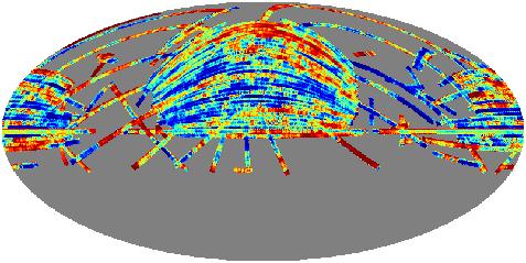
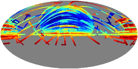
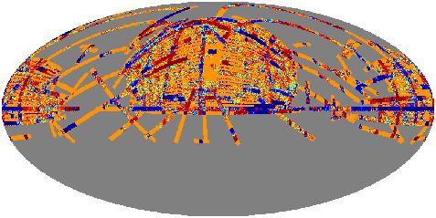
91 Figure 3.2: Templates of the main systematics selected as potential contaminants in the photometric quasar catalogues, and used within the extended mode projection approach. Apart from the first row, all systematics are mapped in the ugriz bands and included in the analysis, but only templates for the i band are shown here. More details can be found in the text, and the full descriptions of the nature and units of these quantities (only referred to by their abbreviated names in this paper) can be found in the SDSS database and documentation. 90

92 Figure 3.3: A subset of systematics templates originating from the decorrelation (using Mask 1) of the basic set of systematics, a subset of which is presented in Fig quasars suffer from large uncertainties (typically σ(ẑ phot ) 0.3) and large fractions of outliers (see e.g., Bovy et al. 2012; Richards et al. 2009). In the present case, the actual n(z) of the quasar samples extend significantly beyond the windows used to construct them. This not only introduces uncertainties in the theoretical predictions, but also cosmological information in the cross-power spectra, since the n(z) of the samples are likely to overlap with each other, as detailed in the next sections. One solution to reduce the associated uncertainties is to employ low-resolution histograms, which are more robust to individual photo-z uncertainties, but do not capture all the structure of the underlying n(z). Alternative methods also exist to attempt to estimate high-resolution n(z) from the poorly-determined photometric redshifts (e.g., Matthews and Newman 2010; McQuinn and White 2013). In Leistedt et al. (2013), we used a cross-matching technique to obtain unbiased estimates for the n(z) of the Richards et al. (2009) catalogue SDSS DR6 photometric quasars. In our case the XDQSOz catalogue includes posterior distributions for the redshift estimates of individual objects, which are computed with the same data-driven model used for the classification, and trained with the best spectroscopic data available. Hence, a simple estimator for n(z) is the sum of the posterior distributions of the individual objects in each sample. Fig. 3.1 shows the resulting n(z), as well as a fit using a superposition of Gaussian kernels for use in CAMB SOURCES. We also show the redshift histograms of cross-matched catalogues of quasars found in catalogues of spectroscopically-confirmed quasars from SDSS DR7 and BOSS DR9 (Pâris et al., 2012; Schneider 91

93 et al., 2010). We applied the relevant flags and cuts to create spatially-uniform versions of these catalogues, i.e., with constant depth, in order to avoid spurious selection effects due to depth variations. However, SDSS DR7 mostly contains bright objects, and BOSS DR9 is dominated by z > 2.2 quasars. Therefore the dashed redshift histograms shown in Fig. 3.1 are biased estimates of n(z), but nevertheless confirm the features found in the XDQSOz n(z). In particular, all four samples contain low-redshift quasars (z ), mainly because of their large scatter in ugriz colour space which overlaps with that of higher redshift quasars hence the difficulty of separating them (Bovy et al., 2011a). The corrections required to follow Leistedt et al. (2013) and obtain unbiased n(z) estimates through cross-matching are more difficult to calculate for XDQSOz than the Richards et al. (2009) catalogue, because the former extends to fainter magnitudes and higher redshifts. In particular, using the full spectroscopic catalogue requires spatially-dependent corrections, which are much more uncertain due to sample variance. For these reasons, we did not attempt to derive and apply these corrections, but rather used the n(z) obtained using the stacked XDQSOz redshift posterior distributions. This should provide the most robust solution, since the XD data-driven model has not been demonstrated to suffer from any biases or systematics over the redshift ranges of interest. In this paper, we focus on evaluating the quality of the measurements and the capacity of mode projection to mitigate systematics. Hence, we will fix the parameters used to calculate the theoretical angular power spectra, and also observational parameters such as the shot noise and the bias of quasars. The latter is assumed to be scale-independent and fixed to b(z) = [ 1 + ( ) ] z, (3.12) 2.5 which is consistent with observations (e.g., Porciani and Norberg 2006; Sherwin et al. 2012; Slosar et al. 2008). As shown in subsequent sections, these parameters provide a good fit to the measured power spectra. However, it is essential to consider their uncertainties when testing models and inferring cosmological parameters. Hence, all theoretical and observational parameters will be varied in the companion paper (Leistedt et al., 2014), where we constrain PNG and evaluate the robustness of these constraints to the underlying models and assumptions Masks and systematic uncertainties 92

94 Figure 3.4: Masks constructed for the power spectrum analysis of the XDQSOz samples. Mask 1 (grey + white) and Mask 2 (grey only) are created by applying dust extinction cuts E(B V ) > 0.1 and E(B V ) > 0.08 to the full SDSS DR8 coverage (black region), in addition to the common cuts Psfwidth i > 2.0 and Score> 0.6 to avoid bad quality regions. The main source of systematics in photometric quasar catalogues is stellar contamination, which arises because separating stars from quasars using imaging data is a difficult task. With the P QSO > 0.8 cut, one can expect a significant fraction of the selected photometric quasars to be stars. However this proportion further depends on the redshift range of interest, since the colours of quasars, and thus the separability of the stellar and quasar loci, evolve with redshift. In addition, observing conditions unavoidably vary with time, and thus on the sky, as data are acquired. This affects both the number of detected point sources and the star-quasar separation, thus creating spatially-varying depth and stellar contamination. We have mapped as many of the potential systematics as possible in order to create templates for the mode projection framework. In what follows, we detail the construction of a base set and an extended set of systematics templates, which will be projected out when estimating the quasar power spectra. For Galactic dust extinction, which affects the properties of point sources and photometric colours, we used the maps of E(B V ) from Schlegel et al. (1998) and Planck (Planck Collaboration, 2013e). They differ in some regions of the sky, especially near the Galactic plane, but are correlated, so we include both maps in the set of systematics prepared for extended mode projection. For the stellar density, we constructed a stellar density map from the SDSS DR6 point sources selected with 18.0 < r < 18.5 and i < 21.3, and a second map with an additional cut g r > 1.4 to select red stars (Pullen and Hirata, 2013). We retrieved the data for the calibration and observing conditions from the FIELDS table in the SDSS CAS server. We mapped all quantities on the sky directly on the HEALPIX (Górski et al., 2005) grid, as the quasar maps are also manipulated in this format. This 93

95 solution does not use the exact geometry of the SDSS tiles (which would require the use of the MANGLE software (Hamilton and Tegmark, 2004; Swanson et al., 2008)) but is much faster while being sufficiently accurate on the scales of interest. Fig. 3.2 shows the base set of systematics we include in this study. Apart from the first row, all templates were constructed for the five ugriz bands, and only the i band is shown in Fig Also, the following quantities were not included on the figure for space reasons: ra, dec, run, fields, mjd, mustart, nustart, total, devapcorrection, devapcorrectionerr, devmodelapcorrection, devmodelapcorrectionerr, nfaintobj, nstaroffset. Full details of the nature, description and units of these quantities can be found in the SDSS database and documentation. The total number of templates in this set of base systematics is 220, but after decorrelating these templates only 100 have significant eigenvalues, the others being consistent with numerical noise, i.e., redundant modes in the system of templates. A subset of these orthogonal modes is shown in Fig. 3. With such a small number of modes, all can be projected out when estimating power spectra, since they only generate a small increase in variance V bb. However, this setting will only treat the spurious clustering due to linear combinations of these systematics. The actual contamination signal is likely to be non-linear and therefore may not be effectively eliminated. To consider non-linear contamination model, we create an extended set of templates, also including products of pairs of the base systematics. Once decorrelated, the 22, 000 maps were reduced to 3, 700 modes. Since they are orthogonal modes, projecting out all of them would be equivalent to removing 3, 700 data points in some rotated basis, thus significantly increasing the variance of the estimates. For this reason, we now use the extended mode projection approach to project out only those modes which are significantly correlated with the quasar data, as detailed in the next section. Although extended mode projection considers non-linear contamination models, it is unlikely to fully clean the stellar contamination across the whole survey area, in particular in the worst regions where systematics are significant. Hence, we construct two masks, shown in Fig Both exclude pixels with PSFWIDTH i > 2.0 and SCORE > 0.6. In addition, Mask 1 uses E(B V ) > 0.1 and Mask 2 uses E(B V ) > 0.08, to remove more dusty regions in the South Galactic Cap. The masks were extended to avoid smoothing-induced contamination, as explained in Feeney et al. (2011b) and Leistedt et al. (2013). Note that previous SDSS quasar studies used more aggressive masks (Ho et al., 2013; Leistedt et al., 2013; Pullen and Hirata, 2013), and the point of extended mode projection precisely is to avoid extra sky cuts and obtain finer control over the elimination of contamination by projecting out the relevant systematics. 94

96 Estimation settings and blind mitigation of systematics We used the QML estimator to simultaneously measure the auto- and cross- angular power spectra of the four XDQSOz samples. We used HEALPIX resolution of N side = 64 for all quasar maps, masks and systematics templates in this work, in which case the power spectrum can be estimated accurately up to l max 130, which is a satisfactory band-limit given the noise levels and the sky cuts under consideration, and the computational requirements of the estimator. The choice of the multipole bin size is guided by the variance of the estimates. For most cases we adopted a bin size l = 21 to obtain a good compromise between variance and multipole resolution of the estimated power spectra. We also used l = 15 for the final runs in order to obtain a better resolution on the lowest multipoles, and therefore a better sensitivity to the PNG signal. The resulting constraints on PNG are presented in the companion paper (Leistedt et al., 2014), and are indeed more stringent in that setting. For the fiducial power spectrum priors required for QML, we used the theoretical power spectra detailed in the previous sections. The QML estimator is robust to small changes in these values, especially when measuring the auto- and cross- spectra, which are relatively featureless 6, and simultaneously estimated from the four quasar maps and the full prior covariance matrix. For the power spectrum measurements presented in the next section, we considered three settings for the treatment of systematics (in combination with the two masks of Fig. 3.4): no mode projection ( no mp ), projection of the base set of systematics basic mp, 100 uncorrelated modes), and projection of the extended set plus products of pairs of templates ( ext. mp, 3700 uncorrelated modes). For the latter, we followed our implementation of extended mode projection, and only projected the modes which were significantly correlated with the data. To perform this selection, we cross-correlated the quasar maps with all orthogonal modes using the approximate QML estimator presented in Section 3.3.3, using the same setting as the main estimator (N side = 64, l max = 130, l = 21 or l = 15). The resulting cross-spectra were used as null tests, and we calculated a reduced χ 2 per systematics mode using a simple Gaussian likelihood (Leistedt et al., 2013). Fig. 3.5 shows the comparison of the reduced χ 2 obtained with the optimal and approximate QML estimators detailed in Section 3.3.3, and demonstrates that the latter is sufficiently accurate for the purpose of these null tests. We observe no significant bias, a reasonable scatter around the axis χ 2 opt.qml = χ2 approx.qml, and a small number of outliers. In particular, we see that selecting modes 6 Since quasars span large volumes, the projection integrals weaken features such as the baryon acoustic oscillations. The latter would only be detectable using narrow redshift samples, which cannot be done with XDQSOz due to the large uncertainties of the photometric redshift estimates. 95

97 χ 2 using approx QML χ 2 using exact QML Figure 3.5: Comparison of the reduced χ 2 obtained with the optimal and approximate QML crosscorrelation estimators. Each dot is a value obtained by using both estimators to calculate the cross-spectra between the four quasar samples (colour-coded) and the base set of 220 systematics templates. N N Bin χ Bin 3 Mask 1, l =21 Mask 2, l =21 Mask 2, l = χ 2 N 1400 Bin χ 2 N 600 Bin χ 2 Figure 3.6: Distributions of the reduced χ 2 arising from null tests performed with the cross-power spectra of the four quasar samples (four panels) with the 3700 orthogonal modes of the extended set of systematics templates ( 200 base templates plus products of pairs). The last step of extended mode projection consists of choosing a χ 2 cut to decide which modes will be projected out when estimating the angular power spectra of the quasar samples. 96

98 for mode projection with the cut χ 2 approx.qml > 1 reproduces the selection using a cut χ2 opt.qml > 1 reasonably well, validating the use of the approximate estimator in the null tests. Fig. 3.6 shows the distributions of the reduced χ 2 values obtained by cross-correlating the four quasar maps with the 3700 modes. Interestingly, these distributions can be used to qualitatively evaluate the level of contamination of the samples, and also the effect of masking. In particular, the second and third samples are the least contaminated, and the χ 2 distributions are not improved by using the second mask instead of the first mask, in addition to being robust to the multipole resolution ( l = 21 or l = 15). The null tests also demonstrate that the first and fourth samples are significantly contaminated by systematics, since a large fraction of the modes have large reduced χ 2. Using resolution l = 15 yields even more modes with large χ 2, because the cross spectra are able to extract features due to systematics which were not discernible with l = 21. In the next section, all power spectra calculated with extended mode projection were computed by projecting out modes with χ 2 > 1. One can adjust this parameter to set the accepted level of correlation between with the data and the templates, above which modes are considered as contaminated by systematics and are projected out. One or multiple values for the χ 2 cut should be decided before the analysis, so that the systematics mitigation relies on objective criteria, and is performed in a blind fashion. Alternatively, iterating and refining the χ 2 cut during the analysis could improve the systematics mitigation, but may also yield fine-tuning and over-processing of the data if the results do not conform to expectation (confirmation bias), jeopardising the search for new physics. We finally note that previous analyses of SDSS quasars (e.g., Pullen and Hirata 2013) used samples with redshift distributions that were not overlapping: therefore their cross-power spectra could be used as null tests, i.e., any systematics in common between the quasar samples would be detectable in the cross-spectra between redshift bins, which should be consistent with zero in the absence of systematics. In this work, the redshift distributions of the quasar samples overlap, some of them significantly, implying that the cross-spectra will contain cosmological information. We will demonstrate in the next section and the companion paper (Leistedt et al., 2014) that the fourth sample is not only the one with the most constraining power for PNG, but also the one with the redshift distribution overlapping the least with the other samples: its cross-power spectra can thus be used for approximate null tests Power spectrum measurements 97

99 10 4 lc l 10 4 lc l 10 4 lc l 10 4 lc l Bin 1 / Bin l Bin 2 / Bin l Bin 3 / Bin l Bin 4 / Bin l 10 4 lc l 10 4 lc l 10 4 lc l Theory, f NL = 0 Theory, -50< f NL < 50 Mask 1, l =21, no mp Mask 2, l =21, no mp Mask 2, l =21, basic mp Bin 2 / Bin l Bin 3 / Bin l Bin 4 / Bin l 10 4 lc l 10 4 lc l Bin 3 / Bin l Bin 4 / Bin l 10 4 lc l Bin 4 / Bin l Figure 3.7: Auto- and cross-angular power spectra of the four XDQSOz quasar samples measured with the quadratic maximum likelihood (QML) estimator, for the two masks in Fig. 3.4, without ( no mp ) and with ( basic mp ) mode projection of the base set of systematics (220 templates from the SDSS FIELDS table, shown in Fig. 3.2). The solid lines show our fiducial theoretical power spectra from a Planck best-fit cosmology and f NL = 0, and the shaded bands show the excursion region allowed when varying f NL in [ 50, 50] (see text for details). 98

100 10 4 lc l 10 4 lc l 10 4 lc l 10 4 lc l Bin 1 / Bin l Bin 2 / Bin l Bin 3 / Bin l Bin 4 / Bin l 10 4 lc l 10 4 lc l 10 4 lc l Theory, f NL = 0 Theory, -50< f NL < 50 Mask 2, l =21, ext. mp (null tests with l =21) Mask 2, l =15, ext. mp (null tests with l =21) Mask 2, l =15, ext. mp (null tests with l =15) Bin 2 / Bin l Bin 3 / Bin l Bin 4 / Bin l 10 4 lc l 10 4 lc l Bin 3 / Bin l Bin 4 / Bin l 10 4 lc l Bin 4 / Bin l Figure 3.8: Same as Fig. 3.7, but using extended mode projection. We used a non-linear contamination model incorporating the base set of systematics templates and also pairs of products of templates, yielding 22, 000 templates: but only 3, 700 orthogonal spatial modes remained after decorrelation. We calculated QML cross-angular power spectra to perform null-tests and calculated reduced χ 2, as shown in Fig

101 Fig. 3.7 shows the results of the QML estimator applied to the quasar samples in three settings: Masks 1 and 2 without mode projection, and Mask 2 with mode projection of the base set of systematics templates. The black lines show our fiducial theoretical predictions, detailed in the previous section. The shaded band indicates the zone spanned by the theory curves when varying PNG in 50 < f NL < 50. Note that all spectra are dimensionless, since they relate to overdensity maps. At first examination, we see that all measured power spectra exhibit significant excess power on a range of scales compared to the theoretical expectation. In particular, the first and the fourth samples (the low and high redshift quasar samples) are in significant disagreement with the theoretical curve. The quasar cross-power spectra also exhibit power excesses, pointing to the presence of significant systematics and spatially-varying stellar contamination in these samples. Qualitatively, the discrepancy between the measurements and the prediction agrees with the levels of contamination measured by the null test χ 2 histograms of the previous section, indicating that at least some of the systematics responsible for the excesses are included in the sets of templates prepared for mode projection. Indeed, the third set of spectra of Fig. 3.7 show that using the basic mode projection significantly decreases the power excesses in the auto-spectra, especially that of the fourth sample. The autopower spectra are now subject to an offset compared to the theoretical predictions. Although this could be due to inadequate cosmological or observational parameters in the predictions, such as underestimated biases, significant excess power in the cross-power spectra indicates that part of the remaining discrepancies must be due to systematics. In the formalism of Section 3.3.2, this also demonstrates that a linear model of the basic set of systematics ( 100 uncorrelated modes) is insufficient to describe the contamination signal and spurious clustering. Moreover, since the error bars of Fig. 3.7 only include cosmic variance and shot noise, we deduce that the contamination level is so large that it prevents any reliable measurement of the quasar bias and PNG. In fact, constraining 7 PNG from the measurements of Fig. 3.7 (ignoring the null test cross-spectra and thus the evidence for high levels of systematics) would yield very large levels of PNG, significantly above the limits set by previous studies of SDSS quasars, luminous red galaxies (LRGs), and in the CMB (e.g., Giannantonio et al. 2014; Planck Collaboration 2013h). The purpose of extended mode projection is precisely to address these issues, and reduce the levels of systematics below the statistical uncertainties by marginalising over the most contaminated modes. 7 The error bars of Fig. 3.7 use the fiducial priors and are included to illustrate the large discrepancies and power excesses due to systematics. To exploit these power spectra in a likelihood analysis, one would need to recompute the covariance matrices around the best-fit theoretical power spectra, which were done for the cleanest power spectrum estimates of Fig

102 Fig. 3.8 shows three sets of estimates obtained when using extended mode projection with the more restrictive mask (Mask 2). The first set of spectra are calculated using band powers of width l = 21 for both quasar spectra and null tests, the third set uses l = 15 for both, and the second set is an intermediate setting where the quasar spectra use l = 15 and the null tests l = 21. This hybrid case is to check the robustness of the final spectra, since we observed in Fig. 3.6 that the null tests with l = 21 and l = 15 yielded slightly different χ 2 distributions for the first and fourth (most contaminated) quasar samples. Firstly, we see that the three settings are in good overall agreement with each other, and also with the fiducial theoretical predictions, as demonstrated by the χ 2 values presented in Table 3.1. Indeed, despite a few band-powers that seem discrepant with the theory predictions at the 1 2σ level when examining Fig. 3.8, the values of the probability to exceed (PTE) show that the fiducial spectra are good fits to the measurements. This indicates that extended mode projection succeeds at mitigating the most important systematics and reduce the contamination to a level below the statistical uncertainties. Interestingly, the multipole resolution l = 21 yields better χ 2 than l = 15. This can be explained by the fact that some systematics had their correlation signatures averaged and smoothed out at l = 21, but resolved at l = 15. In other words, greater multipole resolution generally uncovers more systematics, and may require the use of more numerous or more complex combinations of systematics templates. But for the three sets of spectra shown in Fig. 3.8, none of the low-l band powers in the auto- and cross-power spectra exhibit evidence for systematics. Therefore we conclude that they are suitable for cosmological inference and for constraining PNG, which produces a signal that is more pronounced on large scales. Indeed, the error bars and shaded bands of Fig. 3.8 demonstrate that the clean power spectra will be able to constrain PNG Conclusion Photometric quasar surveys are deep and span extended redshift ranges, which allows us to probe the largest scales of the universe, and therefore test physics which is not well constrained by galaxy surveys. In particular, they can be used to constrain PNG, which is expected to enhance quasar clustering on large scales and leave a characteristic scale-dependent signature in the quasar bias. However, this requires accurate power spectrum measurements, which are compromised by the presence of numerous observational systematics, creating spurious correlations which can mimic 101

103 Table 3.1: The chi-square values for the power spectra measured using extended mode projection with Mask 2 with χ 2 cut = 1.0, presented in Fig The theory curves use Planck ΛCDM cosmology, f NL = 0, and fiducial linear bias b(z) = 1 + [(1 + z)/2.5] 5. The numbers of degrees of freedom are ν p = 7 and ν p = 9 for l = 21 and l = 15, respectively. The probability to exceed (PTE) the observed chi squares are shown in parentheses. Note that PTE < 1% corresponds to χ 2 7 = 18.4 and χ 2 9 = C l estimator: l = 21 l = 15 l = 15 Ext. mp null tests: l = 21 l = 21 l = 15 Bin 1 auto 4.81 (0.682) 7.42 (0.593) 7.66 (0.568) Bin 2 Bin (0.319) 6.13 (0.727) 5.67 (0.772) Bin 2 auto 3.89 (0.792) 4.79 (0.852) 6.23 (0.716) Bin 3 Bin (0.341) (0.180) (0.304) Bin 3 Bin (0.948) 4.02 (0.909) 9.50 (0.392) Bin 3 auto 0.76 (0.997) 6.39 (0.699) 9.16 (0.423) Bin 4 Bin (0.296) (0.137) (0.296) Bin 4 Bin (0.230) (0.162) (0.045) Bin 4 Bin (0.559) 7.55 (0.579) (0.165) Bin 4 auto 3.44 (0.8411) 3.14 (0.958) 4.07 (0.906) the signatures of new physics. We have introduced the extended mode projection technique to robustly mitigate the impact of large numbers of systematics when estimating angular power spectra, and applied it to the photometric quasars from the SDSS XDQSOz catalogue. This technique only relies on the ability to map known and potential sources of systematics on the sky, and cross-correlate them with the data of interest. Previous studies of XDQSOz data required stringent quality and sky cuts, and even the removal of band-powers in order to avoid excessive contamination by systematics. In our analysis, we have used minimal sky cuts, and applied the extended mode projection approach using a large number of systematics templates. Mode projection is equivalent to a Bayesian marginalisation over the amplitudes of the modes of the contamination model when estimating the power spectra. The base set of templates included 220 potential systematics found in the SDSS database, and we have also included products of pairs of templates, leading to a total of 22, 000 systematics templates, yielding a non-linear model for the contamination signal. We have then decorrelated the systematics, and cross-correlated the resulting 3, 700 orthogonal modes with the quasar samples to carry out null tests and detect the modes which most likely create spurious correlations in the data. We have finally estimated clean quasar power spectra by projecting out the modes which yielded reduced χ 2 > 1 for the cross-spectrum null tests. Our pool of systematics and resulting contamination model was very general, and the sky masks minimal; thus, the reduced χ 2 cut is the only tuneable parameter in the extended mode projection approach. Our approach is therefore 102

104 based on the principles of blind analysis, since projecting out modes with reduced χ 2 > 1 is a simple and pre-selected criterion for the accepted level of correlation between the systematics and the maps, which does not depend on the intrinsic clustering of quasars. Using various settings for both the power spectrum estimation and the systematics mitigation, we have tested that the power spectrum measurements are robust to these choices, and consistent with the theoretical predictions. In a companion paper (Leistedt et al., 2014), we show that these spectra, used in a combined likelihood function, yield stringent and robust constraints on PNG and on the bias of quasars. In particular, the constraints separately derived using the auto- and cross-spectra are consistent with each other, and robust to the underlying model and assumptions, for example to the uncertainties in the redshift distributions of the samples. This demonstrates that the remaining levels of correlations created by systematics are below the statistical uncertainties, and that the quasar power spectra are suitable for use in cosmological inferences. Future galaxy and quasar survey data will reach unprecedented precision, and will require accurate mitigation of large numbers of systematics. For instance DES, Euclid (Amendola et al., 2013), and LSST (Abell et al., 2009) will observe hundreds of millions of objects, and probe extended redshift ranges and finer angular scales. This makes them very promising for testing new physics beyond the standard cosmological model, such as PNG, the neutrino sector, dark energy phenomenology, and modifications to General Relativity. At such precision levels, and given that these new physics signatures are typically small deviations from the standard model, power spectrum measurements will be highly sensitive to any systematics. The extended mode projection framework is a good candidate for mitigating such systematics in a robust and blind fashion, while extracting as much information as possible from the hard-won data Acknowledgements We are grateful to Jo Bovy, David Hogg and Adam Myers for sharing the XDQSOz catalogue with us. We also thank Daniel Mortlock, Nina Roth, Filipe Abdalla, Aurélien Benoit-Lévy, and Blake Sherwin, for useful discussions and comments. BL is supported by the Perren Fund and the IMPACT Fund. HVP is supported by STFC and the European Research Council under the European Community s Seventh Framework Programme (FP7/ ) / ERC grant agreement no CosmicDawn. 103

105 We acknowledge use of the following public software packages: HEALPIX (Górski et al., 2005) and CAMB SOURCES (Challinor and Lewis, 2011). We acknowledge use of the Legacy Archive for Microwave Background Data Analysis (LAMBDA). Support for LAMBDA is provided by the NASA Office of Space Science. This work is based on observations obtained with SDSS. Funding for the SDSS and SDSS-II has been provided by the Alfred P. Sloan Foundation, the Participating Institutions, the National Science Foundation, the U.S. Department of Energy, the National Aeronautics and Space Administration, the Japanese Monbukagakusho, the Max Planck Society, and the Higher Education Funding Council for England. The SDSS Web Site is The SDSS is managed by the Astrophysical Research Consortium for the Participating Institutions. The Participating Institutions are the American Museum of Natural History, Astrophysical Institute Potsdam, University of Basel, University of Cambridge, Case Western Reserve University, University of Chicago, Drexel University, Fermilab, the Institute for Advanced Study, the Japan Participation Group, Johns Hopkins University, the Joint Institute for Nuclear Astrophysics, the Kavli Institute for Particle Astrophysics and Cosmology, the Korean Scientist Group, the Chinese Academy of Sciences (LAMOST), Los Alamos National Laboratory, the Max-Planck-Institute for Astronomy (MPIA), the Max-Planck-Institute for Astrophysics (MPA), New Mexico State University, Ohio State University, University of Pittsburgh, University of Portsmouth, Princeton University, the United States Naval Observatory, and the University of Washington. 104

106 4 Constraints on primordial non-gaussianity from 800,000 photometric quasars No one trusts a model except the man who wrote it; everyone trusts an observation, except the man who made it. H. Shapley 4.1. Abstract We derive robust constraints on primordial non-gaussianity (PNG) using the clustering of 800,000 photometric quasars from the Sloan Digital Sky Survey in the redshift range 0.5 < z < 3.5. These measurements rely on the novel technique of extended mode projection to control the impact of spatially-varying systematics in a robust fashion, making use of blind analysis techniques. This allows the accurate measurement of quasar halo bias at the largest scales, while discarding as little as possible of the data. The standard local-type PNG parameters f NL and g NL both imprint a k 2 scale-dependent effect in the bias. Constraining these individually, we obtain 49 < f NL < 31 and < g NL < , while their joint constraints lead to 105 < f NL < 72 and < g NL < (all at 95% CL). Introducing a running parameter n fnl to constrain b(k) k 2+n f NL and a generalised PNG amplitude f NL, we obtain 45.5 exp(3.7 n fnl ) < f NL < 34.4 exp(3.3 n fnl ) at 95% CL. These results incorporate uncertainties in the cosmological parameters, redshift distributions, shot noise, and the bias prescription used to relate the quasar clustering to the underlying dark matter. These are the strongest constraints obtained to date on PNG using a single population of large-scale structure tracers, and are already at the level of pre-planck constraints from the cosmic microwave background. A conservative forecast for a Large Synoptic Survey Telescope-like 105

107 survey incorporating mode projection yields σ(f NL ) 5 competitive with the Planck result highlighting the power of upcoming large scale structure surveys to probe the initial conditions of the universe Introduction Canonical single-field slow-roll inflation predicts initial conditions for structure formation that are essentially Gaussian (Acquaviva et al., 2003; Allen et al., 1987; Babich et al., 2004; Bartolo et al., 2004; Falk et al., 1993; Gangui and Martin, 2000; Gangui et al., 1994; Komatsu and Spergel, 2001; Maldacena, 2003; Salopek and Bond, 1990; Verde et al., 2000; Wang and Kamionkowski, 2000). Any measurement of deviations from this prediction summarised by the term primordial non-gaussianity (PNG) can thus provide evidence for non-standard inflationary physics. One of the most physically interesting forms of PNG is the so-called local model, where the primordial potential φ is modified by including higher order terms, Φ = φ + f NL [φ 2 φ 2 ] + g NL [φ 3 3φ φ 2 ], (4.1) where all fields are evaluated at the same spatial coordinate, and f NL and g NL are real-valued constants (often called the skewness and kurtosis parameters). The most stringent constraints on PNG currently come from higher-order statistics of the cosmic microwave background (CMB). Most recently, the Planck collaboration reported 8.9 < f NL < 14.3 (95% CL) (Planck Collaboration, 2013h), while constraints on the kurtosis have been obtained from the WMAP satellite: < g NL < (WMAP5, 95% CL) (Smidt et al., 2010), or g NL = ( 4.3 ± 2.3) 10 5 (WMAP9, 68% CL) (Regan et al., 2013), g NL = ( 3.3 ± 2.2) 10 5 (WMAP9, 68% CL) (Sekiguchi and Sugiyama, 2013). While these results are compatible with Gaussian initial conditions, their uncertainties still leave room for non-standard inflation models. The unknown relation (bias) between the dark matter density field and a set of observed tracers (which inhabit dark matter halos) is generally considered to be a complication in constraining cosmological parameters from large-scale structure (LSS) data. However, in the case of PNG, the bias is actually an advantage that can be used to distinguish between non-gaussianity in the initial conditions and that generated through late-time non-linear structure formation. PNG introduces a distinctive k-dependence into the halo bias; qualitatively, the bias for local-type PNG scales as 106

108 b(k) k 2 (Dalal et al., 2008; Desjacques and Seljak, 2010b; Matarrese and Verde, 2008; Slosar et al., 2008; Smith et al., 2012). This implies that the strongest signal can be expected on large scales (small k), accessible to wide-area galaxy surveys. At these scales, the bias can be well-approximated by a multiplicative factor between the dark matter- and galaxy power spectra. LSS clustering constraints on PNG provide an independent validation of the CMB results, and are predicted to improve significantly with on-going and future LSS surveys, eventually surpassing CMB constraints if systematic errors can be controlled (Carbone et al., 2008; Desjacques and Seljak, 2010a; Giannantonio et al., 2012; Hamaus et al., 2011; Lidz et al., 2013; Mao et al., 2013; Marian et al., 2011; Pillepich et al., 2012). Quasars the bright nuclei at the centre of the most active galaxies are highly-biased tracers of the LSS, spanning large volumes and covering extended redshift ranges: in principle, quasar surveys are ideal for constraining PNG Giannantonio et al. (2014); Slosar et al. (2008). However, previous analyses have been complicated by the presence of spurious excess power at large scales due to systematics, which mimic the signature of PNG (Giannantonio et al., 2014; Leistedt and Peiris, 2014; Leistedt et al., 2013; Pullen and Hirata, 2013; Xia et al., 2009, 2011). In this Letter, we use a large sample of quasars (Bovy et al., 2012) from the Sloan Digital Sky Survey (SDSS) (Gunn et al., 2006) to constrain PNG. Using a novel technique for blind mitigation of systematics described in Leistedt and Peiris (2014), we are able to significantly enhance the constraining power of the dataset, resulting in PNG constraints from a single LSS dataset which are competitive with those from the CMB. Our results represent a significant step toward achieving the exquisite control of systematics necessary to exploit future LSS surveys to measure PNG PNG with photometric quasars The first LSS constraints on PNG were derived in Slosar et al. (2008) using a combination of tracers from early SDSS releases, leading to f NL = (68% CL). Among these tracers, the photometric quasars candidate quasars identified using imaging data only have the highest bias and probe the largest volume. Therefore, they had the most constraining power (f NL = at 68% CL), demonstrating their potential to constrain PNG and complement CMB experiments. However, subsequent analyses (Giannantonio et al., 2014; Xia et al., 2009, 2011) of photometric quasars from the Sixth SDSS Data Release (using the catalogue from Richards et al. 2009) also revealed 107

109 systematic effects, such as spatially-varying depth and stellar contamination, which could strongly bias the clustering measurements on the largest scales and jeopardise cosmological inferences if not properly mitigated (Leistedt et al., 2013; Pullen and Hirata, 2013). Giannantonio and Percival (2014); Giannantonio et al. (2014) obtained f NL = 5 ± 21 (68% CL) using a range of LSS probes, discarding the auto-correlation of quasars to avoid the main systematic contamination. Ho et al. (2013) used the latest catalogue of SDSS photometric quasars, XDQSOz (Bovy et al., 2011a, 2012), to obtain f NL = (68% CL), and f NL = (68% CL) when combined with constraints from the clustering of Luminous Red Galaxies, relying however on stringent quality cuts on the survey maps and power spectra to limit the impact of systematics. Therefore, photometric quasars have thus far remained underexploited for PNG, as systematics are handled by removing hard-won data XDQSOz power spectrum measurements A different approach was adopted by two of us in Leistedt and Peiris (2014), where the SDSS XDQSOz catalogue was analysed with minimal quality and sky cuts, leading to a sample of 800, 000 quasars covering 8300 deg 2 (compared to 400, , 000 objects used by previous analyses). This base sample was further separated into four redshift bins by selecting objects with photometric redshift estimates ẑ p in top-hat windows [0.5, 1.35], [1.35, 1.7], [1.7, 2.2], [2.2, 3.5]. A quadratic maximum likelihood Bond et al. (1998); Tegmark (1997) method was used to simultaneously estimate the auto- and cross-angular power spectra of the z-binned data. To mitigate the impact of systematics in these power spectra, Leistedt and Peiris (2014) introduced a novel technique, extended mode projection, relying on the fact that most potential systematics (e.g., observing conditions, calibration) were also measured during SDSS observations, and could therefore be mapped onto the sky. We constructed a non-linear, data-driven model of systematics, using 3,700 orthogonal templates obtained by decorrelating 20,000 maps of potential contaminants, including 200 base templates constructed from SDSS data and products of pairs. These orthogonal templates were cross-correlated with the XQDSOz data, yielding null tests which are used to select the most significant systematics following the principles of blind analysis. These were then marginalised over via mode projection (Leistedt et al., 2013; Pullen and Hirata, 2013; Slosar et al., 2004; Tegmark, 108

110 Figure 4.1: Redshift distributions of the four quasar samples used in this analysis, parametrised as superpositions of normal distributions. The shaded regions show the 1, 2 and 3σ regions explored when adding 5% uncertainty to the parameters of these fits, which are included in the MCMC analysis. 1997; Tegmark et al., 1998; Wandelt et al., 2004) in the power spectrum estimator, self-consistently enhancing the estimator variance. This approach allows precision control over systematics, and yields robust measurements of the angular power spectra of XDQSOz quasars, even at the largest angular scales. We now turn to the ingredients and models needed to connect the power spectrum measurements to theoretical predictions and constrain PNG. The redshift distributions n(z) of the four quasar samples, shown in Fig. 4.1, were estimated in Leistedt and Peiris (2014) by stacking the posterior distributions of the individual photometric quasars, and then fit with a superposition of Gaussians. Here, we also added a 5% Gaussian uncertainty on the parameters of this fit (illustrated by the shaded bands in Fig. 4.1) which propagates into the final uncertainties in the PNG parameters. The shot noise was measured in each sample from the average surface density of photometric quasars, but is also subject to uncertainties due to the unknown fraction of stars in the samples between 0 and 20% from the quality cuts applied to XDQSOz (Leistedt and Peiris, 2014). Since non-zero stellar contamination reduces the shot noise, we also marginalised over this effect when constraining PNG. 109

111 Figure 4.2: Constraints on the quasar bias model described in Eq The solid line shows the fiducial model with b 0 = 1, β = 5, and the shaded bands show the 1σ constraints (b 0 = 0.96 ± 0.15, 68% CL, β and f NL marginalised) from the XDQSOz power spectra when varying the bias and PNG parameters, the shot noise, and the redshift distributions. The coloured bands show the results when fixing β = 5 and allowing a different bias amplitude in each redshift bin, to demonstrate the ability of the overall model to simultaneously describe the four samples Halo bias from PNG The impact of local-type PNG is to modify the halo bias by adding a k-dependent term to the Gaussian bias b G (z) (Dalal et al., 2008; Desjacques and Seljak, 2010b; Matarrese and Verde, 2008; Slosar et al., 2008; Smith et al., 2012) b NG (k, z) = b G (z) + β f (z)f NL + β g (z)g NL. (4.2) α(k, z) Here, we neglect an additional small contribution induced by the effect of PNG on the halo mass function, which is independent of k and can thus be absorbed in b G (z). Note that we have also suppressed the implicit mass dependence of b G, β f, and β g in the previous equation. The exact expression for α(k, z) and fitting functions for β f and β g can be found in Smith et al. (2012). A simple extension of the local model is the introduction of a spectral index n fnl in the f NL - generated scale-dependent bias (Agarwal et al., 2014b; Agullo and Shandera, 2012; Dias et al., 2013; Giannantonio et al., 2014; Wagner and Verde, 2012), i.e., changing its scaling from k 2 into k 2+n f NL by using ( ) nfnl k α(k, z) α(k, z), (4.3) k piv 110

112 (b 0,β) (b 1 4 ) (b 1 4 ) +n(z)+cosmo (b 0,β) +n(z) (b 0,β) +cosmo (b 0,β) +n(z)+cosmo f NL Figure 4.3: Constraints on local-type f NL (in the ΛCDM+f NL model, with n fnl = g NL = 0) using the power spectrum analysis of XDQSOz quasars, for different bias models and incorporating uncertainties in the redshift distributions and cosmological parameters. The error bars show the 1 and 2σ constraints, the dashed line shows f NL = 0, and the shaded bands show the constraints from Planck (Planck Collaboration, 2013h). where we choose k piv = 0.06 Mpc 1. Note that this parametrisation is not equivalent to an intrinsically scale-dependent f NL as described in Becker et al. (2011, 2012). Instead, it allows us to extend our analysis to other types of PNG, like that generated by single-field inflation with a modified initial state Agullo and Shandera (2012), or models with several light fields (Dias et al., 2013). The quasar bias is known to evolve strongly with redshift (e.g., Myers et al. 2006, 2007a,b; Shen et al. 2009; White et al. 2012), and thus one cannot use a constant linear bias per redshift bin due to the extended and complicated redshift distributions shown in Fig For the Gaussian bias b(z) in Eq. 4.2, we used b(z) = b 0 [1 + ( ) ] β 1 + z, (4.4) 2.5 which is in good agreement with previous studies of SDSS quasars (e.g., Porciani and Norberg 2006) Monte Carlo Markov Chain (MCMC) analysis We built a Gaussian likelihood (Leistedt et al., 2013), jointly using the 10 auto- and cross- 111

113 angular power spectra (between redshift bins) estimated in Leistedt and Peiris (2014), at multipole resolution l = 15. The theoretical predictions were calculated using CAMB sources (Challinor and Lewis, 2011), modified to support PNG and our quasar bias model. We used emcee (Foreman-Mackey et al., 2013) to run an MCMC analysis, and sample combinations of the following parameters: Cosmological parameters ( cosmo ): parameters of the base ΛCDM model, with fiducial values and uncertainties corresponding to the constraints from Planck combined with Baryon Acoustic Oscillations (BAO), as in Planck Collaboration (2013g). Bias model: the model described above, with uniform priors b 0 [0, 2] and β [4, 6]. Redshift distributions ( n(z) ): the amplitude and width of the Gaussian functions used to fit the n(z) estimates, with Gaussian priors of 5% 1σ uncertainties around the fiducial values. Additionally, we sampled the slope of number counts, which controls magnification bias, with Gaussian priors centred at the measured value with 5% 1σ uncertainty. Shot noise: we marginalised over the shot noise with a prior [0.8, 1.0] times the value measured from the photometric quasar surface density, in order to account for the unknown (but bounded) amount of stellar contamination Results We first test the robustness of the bias model by examining the bias measured in the four redshift samples individually and jointly. Therefore, in addition to the coupled model presented above, used to connect all power spectra to the theory predictions, we consider an alternative, decoupled case where the bias amplitude of each redshift sample is fit separately, using four parameters b 1, b 2, b 3, b 4. In this case, we used β = 5 and uniform priors b i [0, 2]. The constraints on the bias parameters from the XDQSOz power spectra are shown in Fig. 4.2, and demonstrate that the separate bias amplitudes b i, i = of the four samples are in good agreement with each other, with the fiducial model with b 0 = 1 and β = 5 (black line), and also with the results obtained with the coupled model (shaded band). Note that the slope parameter β is used to capture the uncertainty in the evolution of the bias at z > 2.5. This redshift range is not as strongly constrained by the data, but is nevertheless crucial since it has the greatest bias, and therefore is expected to produce the strongest PNG signature. Having confirmed that Eq. 4.4 is an adequate model for the quasar bias, we can now advance towards constraining the PNG parameters. Unless stated otherwise, all values are quoted at 95% CL. 112

114 f NL g NL Figure 4.4: 1σ and 2σ joint constraints on f NL and g NL for the (b 0, β) + n(z)+cosmo case, i.e., marginalising over the uncertainties in the cosmological parameters, redshift distributions, and bias model fnl n fnl Figure 4.5: 1σ and 2σ joint constraints on f NL and n fnl for the extended model of Eq. 4.3, marginalising over the same parameters as Fig

115 Model f NL g NL /10 5 base+f NL base+g NL base+f NL +g NL Table 4.1: PNG constraints for different models. The base model is (b 0, β)+cosmo+n(z). The first super/subscript corresponds to the 68% CL, and the 95% CL can be obtained by adding the second number. Fig. 4.3 shows the constraints on f NL only (with n fnl = g NL = 0) for various combinations of parameters and sources of uncertainties. As expected, adding parameters (e.g., using the decoupled bias model) increases the error estimates. When only varying b 0, β, we obtain 26 < f NL < 34 (top row), and adding the uncertainties in the cosmological parameters and redshift distributions relaxes the constraints to 49 < f NL < 31 (bottom row). Note that this case is more conservative but introduces degeneracies between parameters, in particular those affecting the overall amplitude of the power spectra, such as the bias b 0, the amplitude of matter fluctuations σ 8, and the relative amplitudes of the peaks in n(z). However, f NL does not suffer from any direct degeneracies with these parameters given its specific signature on large scales, yielding constraints which are robust to the choice of model. When only using g NL as a source of scale-dependent bias, we obtain < g NL < However, as apparent from Eq. 4.2, and as shown in Roth and Porciani (2012), f NL and g NL leave similar signatures on the scale-dependent bias of LSS tracers, and are not easily separable. Despite the large volume and extended redshift range spanned by our data, this degeneracy is confirmed by their joint constraints, shown in Fig. 4.4, leading to 105 < f NL < 72 and < g NL < For the extended model of Eq. 4.3, we can introduce a generalised parameter f NL, which only corresponds to f NL as defined in Eq. 4.1 when n fnl = 0. In this model, the scale-dependent bias scales as b(k) k 2+n f NL, so the constraints on f NL widen as n fnl increases, due to the less pronounced signature of PNG on large scales. Nevertheless, f NL can be constrained at any n fnl < 2. Fig. 4.5 shows the joint constraints on f NL and n fnl, summarised as 45.5 exp(3.7 n fnl ) < f NL < 34.4 exp(3.3 n fnl ), fully compatible with f NL =

116 4.8. Future prospects We performed a Fisher forecast of a Large Synoptic Survey Telescope-like photometric survey (LSST Dark Energy Science Collaboration, 2012), using angular power spectra of galaxies in 20 tomographic bins in the redshift range 0.5 < z < 3.5, with bias modelled by b 0 = 1, β = 3 in Eq This idealised forecast, without any contamination by systematics, yields a 1σ uncertainty on f NL of 1, consistent with the 3D power spectrum analysis of Carbone et al. (2008). We then incorporated realistic estimates of the main 50 systematics identified in Leistedt and Peiris (2014). This translates into a 10% clustering contamination for l > 100, up to factors of a few on the largest scales where the PNG signal is strongest. Without any mitigation in the subsequent analysis, the resulting estimate for f NL is biased by f NL 30, which is highly significant compared to the expected uncertainty. Including a harmonic-space mode projection in the forecast removes this bias, while consistently increasing the parameter uncertainty to σ(f NL ) = 5, comparable to current Planck constraints. However, this increase in uncertainty will be significantly reduced when performing the mode projection in pixel space, using sky maps of the systematics which will be available for a real survey (Leistedt and Peiris, 2014; Leistedt et al., 2013) Conclusion Photometric quasar surveys, while potentially constituting ideal datasets for probing PNG, have thus far been systematics-limited. We derived constraints on PNG using the results of a novel power-spectrum estimation method applied to 800, 000 photometric quasars from SDSS. This approach self-consistently marginalises over a non-linear data-driven model of spatially-varying systematics. Our results, summarised in Table 4.1, incorporate uncertainties in the cosmological parameters and the parameters of a realistic bias model, while marginalising over uncertainties in the redshift distributions of the quasars. The resulting constraints on f NL and g NL are the tightest obtained using a single population of LSS tracers, and are at the level of pre-planck CMB constraints. Our results demonstrate the potential of future LSS surveys to reach the f NL 1 levels predicted by the simplest models of inflation. 115

117 4.10. Acknowledgments We are grateful to Jo Bovy, David Hogg and Adam Myers for sharing the XDQSOz catalogue with us, and Jo Bovy, Masahiro Takada for useful conversations. BL is supported by the Perren Fund and the IMPACT Fund. HVP and NR are supported by STFC and the European Research Council under the European Community s Seventh Framework Programme (FP7/ ) / ERC grant agreement no CosmicDawn. We acknowledge use of the following public software packages: HEALPIX (Górski et al., 2005) and CAMB SOURCES (Challinor and Lewis, 2011). We acknowledge use of the Legacy Archive for Microwave Background Data Analysis (LAMBDA). Support for LAMBDA is provided by the NASA Office of Space Science. This work is based on observations obtained with SDSS. Funding for the SDSS and SDSS-II has been provided by the Alfred P. Sloan Foundation, the Participating Institutions, the National Science Foundation, the U.S. Department of Energy, the National Aeronautics and Space Administration, the Japanese Monbukagakusho, the Max Planck Society, and the Higher Education Funding Council for England. The SDSS Web Site is 116

118 5 S2LET: A code to perform fast wavelet analysis on the sphere Energy is neither created nor destroyed. It just changes shape. S. Reynolds 5.1. Abstract We describe S2LET, a fast and robust implementation of the scale-discretised wavelet transform on the sphere. Wavelets are constructed through a tiling of the harmonic line and can be used to probe spatially localised, scale-dependent features of signals on the sphere. The reconstruction of a signal from its wavelets coefficients is made exact here through the use of a sampling theorem on the sphere. Moreover, a multiresolution algorithm is presented to capture all information of each wavelet scale in the minimal number of samples on the sphere. In addition S2LET supports the HEALPix pixelisation scheme, in which case the transform is not exact but nevertheless achieves good numerical accuracy. The core routines of S2LET are written in C and have interfaces in Matlab, IDL and Java. Real signals can be written to and read from FITS files and plotted as Mollweide projections. The S2LET code is made publicly available, is extensively documented, and ships with several examples in the four languages supported. At present the code is restricted to axisymmetric wavelets but will be extended to directional, steerable wavelets in a future release. 117

119 5.2. Introduction Signals defined or measured on the sphere arise in numerous disciplines, where analysis techniques defined explicitly on the sphere are now in common use. In particular, wavelets on the sphere (Antoine and Vandergheynst, 1998, 1999; Baldi et al., 2009; Marinucci et al., 2008; McEwen et al., 2006; Narcowich et al., 2006; Starck et al., 2006a; Wiaux et al., 2005, 2006, 2007, 2008; Yeo et al., 2008) have been applied very successfully to problems in astrophysics and cosmology, where data-sets are increasingly large and need to be analysed at high resolution in order to confront accurate theoretical predictions (e.g. Barreiro et al. 2000; Basak and Delabrouille 2012; Cayón et al. 2001; Deriaz et al. 2012; Labatie et al. 2012; Lan and Marinucci 2008; McEwen et al. 2006, 2007a,b, 2008; Pietrobon et al. 2008; Schmitt et al. 2010; Starck et al. 2006b; Vielva et al. 2004, 2006a,b, 2007; Wiaux et al. 2006, 2008). While wavelet theory is well established in Euclidean space (see e.g. Daubechies 1992b), multiple wavelet frameworks have been developed on the sphere, only a fraction of which lead to exact transforms in both the continuous and discrete settings. In fact, discrete methodologies (Schröder and Sweldens, 1995; Sweldens, 1996, 1997) achieve exactness in practice but may not lead to a stable basis on the sphere (Sweldens, 1997). In the continuous setting several constructions are theoretically exact, and have been combined with sampling theorems on the sphere to enable exact reconstruction in the discrete setting also. In particular, scale-discretised wavelets (Wiaux et al., 2008) lean on a tiling of the harmonic line to yield an exact wavelet transform in both the continuous and discrete settings. In the axisymmetric case, the scale-discretised wavelets reduce to needlets (Baldi et al., 2009; Marinucci et al., 2008; Narcowich et al., 2006), which were developed independently using an analogous tiling of the harmonic line. Similarly, the isotropic undecimated wavelet transform (UWT) developed by (Starck et al., 2006a) exploits B-splines of order 3 to cover the harmonic line with filters with greater overlap but nevertheless compact support. In this paper we describe the new publicly available S2LET 1 code to perform the scale-discretised wavelet transform of complex signals on the sphere. At present S2LET is restricted to axisymmetric wavelets (i.e. azimuthally symmetric when centred on the poles) and includes generating functions for axisymmetric scale-discretised wavelets (Wiaux et al., 2008), needlets (Baldi et al., 2009; Marinucci et al., 2008; Narcowich et al., 2006) and B-spline wavelets (Starck et al., 2006a). We intend to extend the code to directional, steerable wavelets and spin functions in a future release

120 The core routines of S2LET are written in C, exploit fast algorithms on the sphere, and have interfaces in Matlab, IDL and Java. We note that many very useful public codes are already available to compute wavelet transforms on the sphere, including isotropic undecimated wavelet, ridgelet and curvelet transforms 2 (Starck et al., 2006a), invertible filter banks 3 (Yeo et al., 2008), needlets (NeedATool 4 ; Pietrobon et al. 2010) and scale-discretised wavelets (S2DW 5 ; Wiaux et al. 2008). S2LET aims primarily to provide a fast and flexible implementation of the scale-discretised transform with exact reconstruction on the sphere using the sampling theorem of McEwen and Wiaux (2011), although it has also been extended to support some of the features of these other codes. Furthermore, particular attention has been paid in the development of S2LET to prove a user-friendly code, supporting multiple programming languages, and which is extensively documented. The remainder of this article is organised as follows. In section 2 we detail the construction of scale-discretised axisymmetric wavelets and the corresponding exact scale-discretised wavelet transform on the sphere. In section 3 we describe the S2LET code, including implementation details, computational complexity and numerical performance. We present a number of simple examples using S2LET in section 4, along with the code to execute them. We conclude in section Wavelets on the sphere We review the construction of scale-discretised wavelets on the sphere through tiling of the harmonic line (Wiaux et al., 2008). Directional, steerable wavelets were also considered by Wiaux et al. (2008), however we restrict our attention to axisymmetric wavelets here. Furthermore, the use of a sampling theorem on the sphere guarantees that spherical harmonic coefficients capture all the information content of band-limited signals, resulting in theoretically exact harmonic and wavelet transforms. One may alternatively adopt samplings of the sphere for which exact quadrature rules do not exist, such as HEALPix (Górski et al., 2005), but which nevertheless exhibit other useful properties, leading to numerically accurate but not theoretically exact transforms

121 Harmonic analysis on the sphere The spherical harmonic decomposition of a square integrable signal f L 2 (S 2 ) on the twodimensional sphere S 2 reads l f(ω) = f lm Y lm (ω), (5.1) l=0 m= l where Y lm are the spherical harmonic functions, which form the canonical orthogonal basis on S 2. The spherical harmonic coefficients f lm, with l N and m Z such that m l, form a dual representation of the signal f in the harmonic basis on the sphere. The angular position ω = (θ, φ) S 2 is specified by colatitude θ [0, π] and longitude φ [0, 2π). The spherical harmonic coefficients are given by f lm = f Y lm = dω(ω)f(ω)ylm(ω), S 2 (5.2) with the surface element dω(ω) = sin θdθdφ. We consider band-limited signals in the spherical harmonic basis, with band-limit L if f lm = 0, l L. For band-limited signals sampling theorems can be invoked so that both forward and inverse transforms can be reduced to finite summations that are theoretically exact. Sampling theorems effectively encode a quadrature rule for the exact evaluation of integrals on the sphere from a finite set of sampling nodes. Various sampling theorems exist in the literature (e.g. Driscoll and Healy 1994; Healy et al. 1996; McEwen and Wiaux 2011). In this work we adopt the McEwen and Wiaux (2011) sampling theorem (hereafter MW), which is based on an equiangular sampling scheme and, for a given band-limit L, requires the lowest number of samples on the sphere of all sampling theorems, namely (L 1)(2L 1) + 1 2L 2 samples (for comparison 4L 2 samples are required by Driscoll and Healy (1994)). Fast algorithms to compute the corresponding spherical harmonic transform scale as O(L 3 ) and are numerically stable to band-limits of at least L = 4096 (McEwen and Wiaux, 2011). The GLESP pixelisation scheme (Doroshkevich et al., 2005) also provides a sampling theorem based on the Gauss-Legendre quadrature, and could be used in place of the MW sampling theorem. However, GLESP uses more samples than Gauss-Legendre quadrature requires, which may lead to an overhead when considering large band-limits and numerous wavelet scales. We focus on the MW sampling scheme to obtain a theoretically exact transform. Alternative sampling schemes that are not based on sampling theorems also exist such as HEALPix (Górski et al., 2005), which is supported by S2LET, MRS and Needatool. HEALPix does not lead to exact transforms on the sphere but the resulting approximate 120

122 transforms nevertheless achieve good accuracy and benefit from other practical advantages, such as equal-area pixels Scale-discretised wavelets on the sphere The scale-discretised wavelet transform allows one to probe spatially localised, scale-dependent content in the signal of interest f L 2 (S 2 ). The j-th wavelet scale W Ψj L 2 (S 2 ) is defined as the convolution of f with the wavelet Ψ j L 2 (S 2 ): W Ψj (ω) (f Ψ j )(ω) f R ω Ψ j dω(ω )f(ω )(R ω Ψ j ) (ω ), (5.3) S 2 where denotes complex conjugation. Convolution on the sphere is defined by the inner product of f with the rotated wavelet R ω Ψ j. We restrict our attention to axisymmetric wavelets, i.e. wavelets that are azimuthally symmetric when centred on the poles. Consequently, the rotation operator R ω is parameterised by angular position ω = (θ, φ) only and not also orientation 6. For the axisymmetric case the spherical harmonic decomposition of W Ψj is then simply given by a weighted product in harmonic space: W Ψj lm = 4π 2l + 1 f lmψ j l0, (5.4) where W Ψj lm = W Ψj Y lm, f lm = f Y lm and Ψ j l0 δ m0 = Ψ j Y lm, and where δ m0 is the Kronecker delta symbol. The wavelet coefficients extract the detail information of the signal only; a scaling function and corresponding scaling coefficients must be introduced to represent the low-frequency (low-l), approximate information of the signal. The scaling coefficients W Φ L 2 (S 2 ) are defined by the convolution of f with the scaling function Φ L 2 (S 2 ): W Φ (ω) (f Φ)(ω) = f R ω Φ, (5.5) or in harmonic space, 4π Wlm Φ = 2l + 1 f lmφ l0, (5.6) 6 As already noted, the extension to directional scale-discretised wavelets has been derived by Wiaux et al. (2008). At present the S2LET code supports axisymmetric wavelets only; directional wavelets will be added in a later release. 121

123 where W Φ lm = W Φ Y lm and Φ l0 δ m0 = Φ Y lm. Provided the wavelets and scaling function satisfy an admissibility property (defined below), the function f may be reconstructed exactly from its wavelet and scaling coefficients by f(ω) = dω(ω )W Φ (ω )(R ω Φ)(ω) S 2 J + dω(ω )W Ψ j (ω )(R ω Ψ j )(ω), (5.7) S 2 j=j 0 or equivalently in harmonic space by 4π 4π f lm = 2l + 1 W lmφ Φ l0 + 2l + 1 J W Ψ j j=j 0 lm Ψ j l0. (5.8) The parameters J 0, J define the lowest and highest scales j of the wavelet decomposition and must be defined consistently to extract and reconstruct all the information content of f. These parameters depend on the construction of the wavelets and scaling function and are defined explicitly in the next paragraphs. The admissibility condition under which a band-limited function f can be decomposed and reconstructed exactly is given by the following resolution of the identity: 4π Φ l l + 1 J j=j 0 Ψ j l0 2 = 1, l. (5.9) We are now in a position to define wavelets and a scaling function that satisfy the admissibility property. In this paper, we use the smooth generating functions defined by Wiaux et al. (2008) in order to tile the harmonic line. Alternative definitions are also supported by S2LET, as presented at the end of this section. Consider the C Schwartz function with compact support on [ 1, 1]: s(t) e 1 1 t 2, t [ 1, 1] 0, t / [ 1, 1], (5.10) for t R. We introduce the positive real parameter λ R + to map s(t) to ( ) 2λ s λ (t) s (t 1/λ) 1, (5.11) λ 1 122

124 which has compact support in [1/λ, 1]. We then define the smoothly decreasing function k λ by k λ (t) 1 dt t 1 1/λ t s 2 λ (t ) dt t s 2 λ (t ), (5.12) which is unity for t < 1/λ, zero for t > 1, and is smoothly decreasing from unity to zero for t [1/λ, 1]. We finally define the wavelet generating function by κ λ (t) k λ (t/λ) k λ (t) (5.13) and the scaling function generating function by η λ (t) k λ (t). (5.14) The wavelets and scaling function are constructed from their generating functions to satisfy the admissibility condition given by Eqn. (6.35). A natural approach is to define Ψ j lm from the generating functions κ λ to have support on [λ j 1, λ j+1 ], yielding Ψ j lm 2l + 1 4π ( ) l κ λ λ j δ m0. (5.15) For these wavelets Eqn. (6.35) is satisfied for l λ J0, where J 0 is the lowest wavelet scale used in the decomposition. The scaling function Φ is constructed to extract the modes that cannot be probed by the wavelets (i.e. modes with l < λ J0 ): Φ lm 2l + 1 4π ( ) l η λ δ m0. (5.16) λ J0 To satisfy exact reconstruction, J is set to ensure the wavelets reach the band-limit of the signal of interest, yielding J = log λ (L 1). The choice of the lowest wavelet scale J 0 is arbitrary, provided that 0 J 0 < J. The wavelets and scaling function may then be reconstructed on the sphere through an inverse spherical harmonic transform. The harmonic tiling and real space representation of these wavelets are shown in Figure 5.1 and Figure 5.2 respectively. In addition to the scale-discretised generating functions (Wiaux et al., 2008), S2LET also supports the needlet functions (Marinucci et al., 2008) 7, which yield a similar tiling of the harmonic line, as shown in Figure 5.1. The B-spline filters used to construct the isotropic undecimated wavelet 7 In our implementation of needlets we use a scaling function to represent the approximate information in the signal, which is not always included (e.g., NeedAtool; Pietrobon et al. 2010). 123

125 Φ l0 Ψ 2 l0 Ψ 3 l0 Ψ 4 l0 Ψ 5 l0 (a) Tiling of the harmonic line l Φ(θ, φ = 0) Ψ 2 (θ, φ = 0) Ψ 3 (θ, φ = 0) θ θ θ (b) Angular profiles of the scaling function and the first wavelets Figure 5.1: Wavelets and scaling function constructed with the scale-discretised (SD), needlet and B-spline generating functions (Marinucci et al., 2008; Starck et al., 2006a; Wiaux et al., 2008) with parameters λ = 3 and J 0 = 2 and for band-limit L = 128. The tiling is shown in the top panel, and the profiles of the reconstructed wavelets in the bottom panel. transform (Starck et al., 2006a) are also supported, as also shown in Figure With these three constructions, the wavelets and scaling functions are well-localised both spatially on the sphere and also in harmonic space. Consequently, the associated wavelet transforms on the sphere can be used to extract spatially localised, scale-dependent features in signals of interest. 8 For the B-spline-based construction to probe approximately the same scales as the scale-discretised and needlet ones, we defined the generating functions as k λ (t) = 3 2 B 3(2 tλj 1 L ) (5.17) 1 B 3 (x) = 12 ( x x x 3 4 x x ), (5.18) so that the jth filter has (compact) support [0, L/λ J j 2 ] and peaks at the same scales as the j-th scale-discretised and needlet filters obtained with the same parameters. 124

126 Φ(ω) Ψ 2 (ω) Ψ 3 (ω) Ψ 4 (ω) Ψ 5 (ω) Figure 5.2: Wavelets for scales j {2, 3, 4, 5} and scaling function constructed through a tiling of the harmonic line using scale-discretised functions, with parameters λ = 3 and J 0 = 2 and for band-limit L = 128. This plot was produced with a Matlab demo included in S2LET The S2LET code In this section we describe the S2LET code. We first introduce a multiresolution algorithm to capture each wavelet scale in the minimum number of samples on the sphere, which follows by taking advantage of the reduced band-limit of the wavelets for scales j < J 1. This multiresolution algorithm reduces the computation cost of the transform considerably. We then provide details of the implementation, the computational complexity and the numerical accuracy of the scale-discretised wavelet transform supported in S2LET. We finally outline planned future extensions of the code Multiresolution algorithm In harmonic space, the wavelet coefficients are simply given by the weighted product of the spherical harmonic coefficients of f and the wavelets, as expressed in Eqn. (6.30). Although the wavelet coefficients can be analysed at the same resolution as the signal f (i.e., at full resolution), by construction they have different band-limits for different scales j, as shown in Figure 5.1. The reconstruction can thus be performed at lower resolution, without any loss of information if a sampling theorem is used. This approach yields a multiresolution algorithm where the wavelet coefficients are reconstructed with the minimal number of samples on the sphere: the j-th wavelet 125

127 coefficients have band-limit k = λ j+1 when using the scale-discretised and needlet kernels, and k = L/λ J j 2 when using the B-splines. When the MW sampling theorem is used, the wavelets are recovered on (k 1)(2k 1) + 1 samples on the sphere. This approach leads to significant improvements in terms of speed and memory use compared to the full-resolution case, as shown in the next section. Figure 5.3 illustrates the use of the full-resolution and multiresolution transforms on a map of Earth topography data with the scale-discretised filters and the MW scheme. When adopting the HEALPix sampling of the sphere, multiresolution can also be used. However HEALPix does not rely on a sampling theorem and therefore the resolution for the reconstruction of each wavelet scale must be chosen heuristically and adapted to the desired accuracy. For example, in the MRS code (Starck et al., 2006a) it is chosen such that N j side = k/2. More detail on the accuracy of the wavelet transform with HEALPix are provided below. (a) Full-resolution scale-discretised wavelet transform (b) Multiresolution scale-discretised wavelet transform Figure 5.3: Scale-discretised wavelet transform of a band-limited topography map of the Earth for λ = 3, J 0 = 2 and L = 128, i.e. with the scale-discretised wavelets shown in Figure 5.2. The wavelet transform decomposes the band-limited signal into wavelet coefficients that extract spatially localised, scale-dependent features. Since the wavelets for different scales j have different band-limits, the wavelet coefficients can be reconstructed at lower resolution on the sphere for lower scales j. Panel (a) shows the full-resolution wavelet transform of the topography map. The original Earth topography map is shown in the top-left plot, the scaling coefficients are shown in the top-right plot, while the wavelet coefficients at scales j {2, 3, 4, 5} are shown left-to-right, top-to-bottom respectively in the remaining plots. Panel (b) shows the same decomposition but using the multiresolution algorithm. The signals shown in panel (b) contain the same information as in panel (a) but represented in the minimal number of samples on the sphere. These plots were produced by one of the many Matlab demos provided with S2LET. 126