arxiv: v1 [astro-ph.sr] 26 Dec 2018
|
|
|
- Josephine Tyler
- 5 years ago
- Views:
Transcription
1 Transition from circular-ribbon to parallel-ribbon flares associated with a bifurcated magnetic flux rope Z. Zhong 1,2, Y. Guo 1,2, M. D. Ding 1,2, C. Fang 1,2, Q. Hao 1,2 1 School of Astronomy and Space Science, Nanjing University, Nanjing , China arxiv: v1 [astro-ph.sr] 26 Dec 2018 guoyang@nju.edu.cn, dmd@nju.edu.cn 2 Key Laboratory for Modern Astronomy and Astrophysics (Nanjing University), Ministry of Education, Nanjing , China ABSTRACT Magnetic flux ropes play a key role in triggering solar flares in the solar atmosphere. In this paper, we investigate the evolution of active region NOAA within 36 hours from 2015 January 29 to 30, during which a flux rope was formed and three M-class and three C-class flares were triggered without coronal mass ejections. During the evolution of the active region, the flare emission seen in the Hα and ultraviolet wavebands changed from a circular shape (plus an adjacent conjugated ribbon and a remote ribbon) to three relatively straight and parallel ribbons. Based on a series of reconstructed nonlinear force-free fields, we find sheared or twisted magnetic field lines and a large-scale quasi-separatrix layer (QSL) associated with 3D null points in a quadrupolar magnetic field. These features always existed and constantly evolved during the two days. The twist of the flux rope was gradually accumulated that eventually led to its instability. Around the flux rope, there were some topological structures, including a bald patch, a hyperbolic flux tube and a torus QSL. We discuss how the particular magnetic structure and its evolution produce the flare emission. In particular, the bifurcation of the flux rope can explain the transition of the flares from circular to parallel ribbons. We propose a two-stage evolution of the magnetic structure and its associated flares. In the first stage, sheared arcades under the domelike large-scale QSL were gradually transformed into a flux rope through magnetic reconnection, which produced the circular ribbon flare. In the second stage, the flux rope bifurcated to form the three relatively straight and parallel flare ribbons. Subject headings: Sun: flares Sun: UV radiation Sun: magnetic field Sun: magnetic topology 1. Introduction Solar flares are one of the most complex dynamic processes in the solar atmosphere, which release a large amount of energy in a wide wavelength range (e.g., Shibata & Magara 2011). They are usually associated with coronal mass ejections (CMEs) ejecting a large amount of magnetized plasmas. The magnetized plasmas along with energetic particles from explosive events propagate through the interplanetary space. They may impact the Earth, resulting in serious space weather conditions (e.g., Gosling et al. 1991; Chen 2011; Cheng et al. 2017). Therefore, it is important to study the origin of solar flares. In two dimensions, the formation and evolution of a flare is usually described by a standard model known as the CSHKP model (Carmichael 1964; Sturrock 1968; Hirayama 1974; Kopp & Pneuman 1976). It states that a magnetic flux rope rises
2 2 due to its instability (or loss of equilibrium), stretches the field lines above, and at the same time, leaves a current sheet behind where magnetic reconnection occurs. The rising flux rope could drive a CME, while the reconnection forms a series of post-flare loops that stride over the magnetic neutral line. Energetic particles can be accelerated during magnetic reconnection and then spiral down along the magnetic field lines to impact the lower atmosphere, where the flare ribbons are formed. Although the standard 2D flare model is quite successful in interpreting some observations, flares indeed occur in three dimensions and show many features that cannot be described by the 2D model (Aulanier et al. 2012). Typical three-dimensional (3D) features include S-shaped coronal sigmoids (e.g., Aulanier et al. 2010), twisted flux ropes (e.g., Canou et al. 2009), sheared and J-shaped flare ribbons (e.g., Cheng & Ding 2016), and circular flare ribbons (e.g., Masson et al. 2009; Sun et al. 2012, 2013; Mandrini et al. 2014). Therefore, extensions of the 2D model, or quasi-3d models were proposed in the past two decades (e.g., Shibata et al. 1995; Tripathi et al. 2006). However, they still cannot explain all the new features revealed by the new observations with increasing resolutions. Recently, Aulanier et al. (2010) revealed the whole process of a flare, in which the formation and eruption of a 3D flux rope plays a key role in the flare process. First, bald-patch (BP) reconnection, driven by flux cancellation, transforms the sheared arcades into a flux rope. Second, due to the slip-running reconnection in the sheared coronal magnetic fields, the flux rope keeps rising and the BP separatrix is gradually transformed into a quasi-separatrix layer. Finally, when the flux rope reaches the critical point of the torus instability, it rises rapidly and triggers the eruption of the CME. In the standard flare model, the stability of the magnetic flux rope determines whether the flare is triggered or not. The magnetic flux rope is a very significant structure in the corona that is defined as helical magnetic field lines wrapping around the central axis with more than one turn. Magnetic flux ropes play important roles in triggering solar flares, driving CMEs, and structuring filaments. Over the past three decades, many authors have contributed to the study of magnetic flux ropes in various aspects including theory (e.g., see review by Forbes 2000), observations (e.g., Cheng et al. 2011; Zhang et al. 2012), and numerical simulations (e.g., Amari et al. 2000, 2003a,b; Inoue & Kusano 2006; Aulanier et al. 2010). In particular, the scientific questions that have been explored include how the magnetic flux rope forms and evolves (Aulanier et al. 2010; Zhang et al. 2012), whether a magnetic flux rope exists before a CME (Chintzoglou et al. 2015), how the magnetic flux rope becomes unstable (Török & Kliem 2003, 2005; Hassanin & Kliem 2016), how the magnetic flux rope breaks out (Antiochos et al. 1999), whether the magnetic flux rope is a necessary condition to produce a CME (Ouyang et al. 2015), and whether the magnetic flux rope is a supporting structure of a filament or not (Guo et al. 2010, 2011). Furthermore, Aulanier et al. (2012) extended the standard flare model to three dimensions, especially on the nature of the strong-to-weak shear transition in post-flare loops by observations and 3D MHD simulations. They provided the pre-eruptive and the post-eruptive distributions of the shear quantitatively. Janvier et al. (2013) further revealed some properties of 3D reconnection by MHD simulations, particularly the slip-running reconnection in quasi-separatrix layers, in eruptive flares. The standard model in three dimensions provides some predictions that have been confirmed by subsequent observations, for instance, a good correspondence between the photospheric footprints of the coronal electric current layer and the flare ribbons (Janvier et al. 2014), and the apparent slip-running reconnection revealed by the motions of flare loops and S-shaped erupting loops in the same direction (Dudík et al. 2014). Moreover, the motions of flare loops and S-shaped erupting loops in opposite directions along flare ribbons are also seen as an apparent slip-running reconnection (Dudík et al. 2016). The standard flare model in three dimensions does not contain null points. Therefore, it cannot explain a special type of flares, called circular ribbon flares, which are usually associated with the spine-fan structure
3 3 and are widely studied recently (e.g., Wang & Liu 2012; Sun et al. 2013; Yang et al. 2015; Masson et al. 2017). Generally speaking, the morphology of a circular ribbon flare comprises a fully closed circular or quasi-circular ribbon, an elongated inner ribbon, and a remote ribbon. Photospheric line-of-sight magnetic field of the circular ribbon flares generally displays a small parasitic polarity being embedded in a main polarity of the opposite sign in an active region. In addition, circular ribbon flares have a special magnetic topology including a 3D null point, whose structure can be analyzed by a Taylor expansion and the Jacobian matrix in the vicinity of it (Parnell et al. 1996). The Jacobian matrix has three eigenvectors corresponding to three eigenvalues, two of which have the same sign determining a fan separatrix, and the third one with the opposite sign defines a spine structure. The circular ribbon, inner ribbon, and remote ribbon are located at the footprints of the fan separatrix, inner spine below the fan separatrix, and the outer spine, respectively. Magnetic reconnection can occur not only in the above configuration to produce circular ribbon flares (e.g., Titov et al. 2002; Guo et al. 2017), but also in other magnetic topological structures, such as bald patches (e.g., Titov et al. 1993; Aulanier et al. 1998; Démoulin et al. 1999), separators (e.g., Longcope 2003; Parnell et al. 2010a,b), and, more commonly, quasi-separatrix layers (QSLs; e.g., Priest & Démoulin 1995; Aulanier et al. 2005). QSLs are defined as places with strong gradients of magnetic connectivity (e.g., Démoulin et al. 1996a,b; Mandrini et al. 1997; Titov et al. 2002; Démoulin 2006). We usually characterize the gradient of magnetic connectivity through a topological parameter called the squashing factor Q (Titov et al. 2002). QSLs are places with a high value of Q, which is much larger than 2. Usually, QSLs appear as narrow layers with finite thickness. When magnetic reconnection occurs, the energetic particles along the field lines impact the footprints of QSLs, which intersect with the chromosphere, to brighten up flare ribbons (Démoulin et al. 1997; Mandrini et al. 1997). These results demonstrate that we can analyze the evolution of flare ribbons to study the field line s linkage although reconnection mostly occurs in the corona. Furthermore, it is worth noting an essential structure called the hyperbolic flux tube (HFT; Titov et al. 2002), which is located at the core of QSLs. The HFT structure is a generalization of a magnetic separator. It situates at the center of a flare region and corresponds to an X-type point in two dimensions, which could release a large amount of energy. Therefore, we can locate the possible position of magnetic reconnection effectively by these topological structures. In some events, magnetic reconnection occurs in complex topologies that contain magnetic flux rope and various topological structures simultaneously. Sun et al. (2013) found that a twisted flux rope exists below the fan structure in a circular-ribbon flare, yet the flare ribbons corresponding to the flux rope do not show a separation due to its small size. Joshi et al. (2015) found, however, a continuous separation between two parallel ribbons in a similar flare. In this event, a compact ribbon, two parallel ribbons, and a quasi-circular ribbon appear successively. They confirmed the existence of a flux rope and a null point. In many cases, multiple flare ribbons with different shapes are produced by complex magnetic topologies, rather than a simple structure such as a sheared two-ribbon flare corresponding to a magnetic flux rope or shear arcades and a circular ribbon flare associated with a null point. It should be noted that magnetic flux rope may not be simply shown as two foot points in the photosphere as we normally observe. A flux rope possibly connects multiple poles, or, to say, the flux rope might be bifurcated toward one or two ends. This is uncommon but actually appears in some observations. In such cases, it is impossible to describe the magnetic structure in two dimensions, while a 3D model is needed. On the other hand, we also need to study the interaction between the null points and the flux rope in order to understand how the flare is initiated and evolves. In this paper, we make a detailed analysis of an active region containing a magnetic flux rope and null points that produced 6 M- and C-class flares from 2015 January 29 to 30. We construct a series of 3D magnetic field using a nonlinear force-free extrapolation and compute the topological structure in terms of
4 4 the squashing factor Q. We then explore the formation of the magnetic flux rope and interpret the Hα and extreme ultraviolet emission properties of the flares. The paper is organized as follows. In section 2, we describe the observations and modeling method. In Section 3, we present the results of the magnetic field and associated flare ribbons, and analyze the magnetic topology. We summarize major findings and give our discussions in Section Observations and modeling 2.1. Overview of the active region The active region NOAA appeared on 2015 January 21 on the east limb of the Sun. At first, it was a simple active region including a negative polarity on the east and a positive polarity on the west. With the cancellation and emergence of the magnetic field, it gradually became a mosaic structure. A parasitic positive polarity appeared that was partially enclosed by the negative polarity on the east. Then, the active region produced the first flare of M1.1 class on January 26. Subsequently, the parasitic positive polarity continued to expand, and the biggest flare of M2.1 class occurred on January 29. Later, two flares of M2.0 and M1.7 class erupted on January 30. Finally, the flare activities decreased and ended at the west limb on February 4. Thus, this region was very active and flare-productive during January 29 and 30 (as shown in Figure 1). Since the active region was located near the central meridian of the Sun, the observed vector magnetic field on the photospheric boundary is accurate enough for further analysis. Here, we analyze the active region for 36 hours from 00:00 UT on January 29 to 12:00 UT on January 30. During this time, six flares (F1 F6) occurred in the active region (as listed in Table 1), which are all above C1.0 class as recorded by the soft-x ray instrument on board the Geostationary Operational Environmental Satellite (GOES). The evolution of the six flares was monitored by the ground-based solar telescope, Optical and Near Infrared Solar Eruption Tracer (ONSET; Fang et al. 2013), and Global Oscillation Network Group (GONG; Harvey et al. 2011) in Hα. The six flares were also observed by the Atmospheric Imaging Assembly (AIA; Lemen et al. 2012) on board the Solar Dynamics Observatory (SDO; Pesnell et al. 2012) with a high temporal cadence (12 s) and spatial resolution ( 0.6 per pixel). Moreover, we carefully check the data observed by the Large Angle and Spectrometric Coronagraph (LASCO) C2 aboard the Solar Heliospheric Observatory (SOHO; Brueckner et al. 1995) and by AIA. We do not find any CME associated with the flares. Thus, the flares in this active region are regarded as confined ones and have attracted a lot of attention (e.g., Hernandez-Perez et al. 2017) Flare emission in Hα and AIA multi-wavelengths During the time interval of 36 hours from January 29, the active region was very productive in flares. From the GOES 1 8 Å soft X-ray emission (Figure 1), we can see that flares larger than C1.0 class (including 3 M-class flares) occurred every six hours on average. Flare ribbons were observed in the Hα and ultraviolet wavelengths corresponding to the chromospheric foot points of flare loops that have been formed by reconnection. These observations thus enable us to trace the morphological evolution of flare ribbons. In addition, the extreme ultraviolet images at 171 and 94 Å from AIA provide another perspective of the active region. The emission of AIA 171 Å originates from the upper transition region and the quiet corona, which contains the Fe ix line emission with a characteristic temperature of K. It usually reveals the low-temperature coronal structures. Different from 171 Å, the 94 Å waveband has a higher characteristic
5 5 temperature of K. It includes the Fe xviii line emission from the flaring corona and is generally used to observe coronal structures with high temperatures. Figure 2a 2f and Figure 3a 3f show the AIA 1600 Å and Hα images of the six flares (F1 F6) at their peak time during the period from 00:00 UT on January 29 to 12:00 UT on January 30. All flare ribbons are labeled as R1 R6 in the AIA 1600 Å images for each flare. Figure 3g 3l shows the six composite snapshots at 171 and 94 Å corresponding to the GOES peak flux times for the six flares. We divide the flare region into three parts: the east part (region E), the middle part (region M) and the west part (region W). The main characteristics of the six flares are summarized as follows. 1. The C8.2 class flare (Figures 2a, 3a, and 3g): In the AIA 1600 Å and Hα images, two ribbons (R1 and R2) on each side of the polarity inversion line (PIL) appeared together at 05:15 UT. The GOES flux reached its maximum at 05:23 UT. Subsequently, the two ribbons began to separate and ribbon R1 (the southern one) got elongated. Finally, the morphology of ribbon R1 changed to a semi-circular shape, and the flare looked like a circular ribbon flare. Ribbon R2 (the northern one) is the adjacent conjugated ribbon. With the evolution of the flare, the foot points of flare loops separated gradually from the PIL. In the AIA 171 Å images, we find a lot of plasma flowing from regions E to M and some faint plasma flowing from regions M to E before the flare onset. Then, after the flare occurred, region M released a high temperature emission at AIA 94 Å rapidly, which extended to both ends. Some plasma appeared flowing to region W simultaneously with the brightening of region M. At the same time, ribbon R3, a remote ribbon, was formed. Although the global picture looks like a circular ribbon flare, the evolution process of ribbons R1 and R2 can also be described by a strong-to-weak shear transition of flare loops predicted in the 3D flare model (Aulanier et al. 2012). 2. The M2.1 class flare (Figures 2b, 3b, and 3h): In this flare F2, the morphology of the flare ribbons was complex owing to multiple ribbons (R1, R2, R3, and R4). The emission characteristics at extreme ultraviolet wavebands were also different from that of flare F1. Some observations have already been described in Hernandez-Perez et al. (2017). In contrast to flare F1, this flare has a much clearer remote ribbon (R4) in region W, and ribbon R2 in region M was not elongated. However, ribbon R1 appeared in region E. As seen in AIA 171 Å, before the flare occurred, there was some plasma moving from regions M to E. Then, in the rising phase, region M released some emissions which extended to both ends in both AIA 94 Å and 171 Å. Moreover, we can see that some coronal loops were opened obviously and more loops were connected to regions M and W in the maximum phase. Meanwhile, the plasma flowed to region W with a wider brightening region than in flare F1. Region E showed a similar phenomenon to region W instead of a successive brightening caused by region M. Hernandez-Perez et al. (2017) interpreted such a phenomenon as magnetic reconnection in region M and plasma flow dissipation in regions E and W. 3. The C6.4 class flare (Figures 2c, 3c, and 3i): For this flare F3, the morphological evolution of the flare ribbons was similar to flare F1. Two ribbons (R2 and R3) also separated from each other during the flare evolution and the shape of the flare tended to be half-circular with the appearance of ribbon R1 in the end. Subsequently, a remote ribbon R4 was formed. However, there were still some differences. On the one hand, in Hα image, ribbons R1 and R2 overlapped each other to form a ribbon that was much wider than ribbon R1 in flare F1. On the other hand, in the AIA multi-wavelength images, the low coronal loop connecting regions M and W had a structure that deviated from a semi-circular shape. Furthermore, high temperature emission at 94 Å appeared not only in region E, but also in region W. 4. The M2.0 class flare (Figures 2d, 3d, and 3j): The morphology of this flare F4 was more complicated
6 6 than the previous flares with four ribbons (R2, R3, R4, and R5) appearing in region M. After the occurrence of the flare, ribbon R2 in region M extended continuously and ribbon R1 was formed in region E. Ribbons R1 and R2 became a semi-circular shape. Meanwhile, a remote ribbon (R6) appeared with a narrow feature. The emission at 94 Å had become visible before the flare occurred. The plasma flowed from the foot point in region M to the two foot points in regions E and W after the flare onset. Then, during the maximum phase, the multiple regions M, E, and W were brightened up at the same time. The flare in region M resembled an inverse S-shaped structure, implying that a flux rope came into existence. In addition, the lower coronal loops connecting regions M and W displayed extremely narrow structures that were different from the former three flares apparently. As a whole, the flare presented a complex structure including six ribbons in total. 5. The C2.3 class flare (Figures 2e, 3e, and 3k): In this flare F5, owing to its weakest strength among the six flares, the brightening of the flare ribbons was not obvious. However, great changes of the ribbon morphology had taken place compared to the aforementioned flares. On the one hand, the flare has three relatively straight and parallel ribbons instead of a circular ribbon (plus an adjacent conjugated ribbon and a remote ribbon). The sizes of each ribbon were closer to each other than the previous flares. We name such a flare as a parallel-ribbon flare hereafter. On the other hand, the distance between ribbons R2 and R3 became smaller than the aforementioned flares. Moreover, both ribbons R2 and R3 evolved to an elongated shape with time. In nor AIA extreme ultraviolet wavebands did the original circular characteristics exist. During the maximum phase, the inverse S-shaped structure in region M became more obvious than in previous cases. In the late phase, the inverse S-shaped structure connected regions M and W with a large amount of 94 Å emissions. The whole structure was transformed into a flare with sheared ribbons. 6. The M1.7 class flare (Figures 2f, 3f, and 3l): This last flare F6 occurred half an hour after flare F5. It shows the apparent characteristics of a three-parallel-ribbon flare. The size of the remote ribbon (R3) was larger than that of the above flares. The morphology of the flare was completely different from that of the circular-ribbon flare. The flare was also different from previous three-ribbon flares in morphology (Wang et al. 2014; Mandrini et al. 2014; Sharykin et al. 2017; Bamba et al. 2017). In our event, although all the three ribbons were near the PIL, they had different sizes and were only roughly parallel to each other. As seen in AIA 94 Å, the inverse S-shaped structure in region M was brightening up instantaneously and released an intense emission during the maximum phase. At the same time, the emission at AIA 171 Å was enhanced to show strong sheared flare loops. Then, region W released some emissions at AIA extreme ultraviolet wavebands, when ribbon R3 was formed Overview of photospheric vector magnetic field and preprocessing The active region was also well observed by the Helioseismic and Magnetic Imager (HMI; Scherrer et al. 2012) on board SDO. SDO/HMI observes the four Stokes profiles (I, Q, U, and V ) of the Fe I 6173 Å line. The photospheric vector magnetic field is derived by fitting the observed Stokes profiles using the Very Fast Inversion of the Stokes Vector (VFISV; Borrero et al. 2011), which is provided by the HMI pipeline (Hoeksema et al. 2014) operated in the Joint Science Operations Center 1. The data for study cover the full solar disk with a temporal cadence of 720 s and a spatial resolution of 1 with a plate scale of
7 7 per pixel (Schou et al. 2012). To analyze the vector magnetic fields, we make two more steps in addition to the processing of the HMI pipeline. First, we need to remove the 180 ambiguity of the transverse field following the minimum energy method (Metcalf 1994; Metcalf et al. 2006; Leka et al. 2009). Second, we should correct the projection effect using the method proposed by Gary & Hagyard (1990) since the active region is not located at the center of solar disk. Here, we coalign each frame of magnetogram to a region at 00:00 UT on January 29. As shown in Figure 3m 3r, we can see the vector magnetic field varying with time from 05:24 UT on January 29 to 05:36 UT on January 30. The overall structure of the active region was roughly maintained during this period. In the east, there was a positive polarity surrounded by a negative polarity, while a large positive polarity appeared in the west. With time elapsing, on the one hand, the parasitic positive polarity in the east was emerging continuously. In particular, the positive and negative polarities showed a sheared structure and were cancelled strongly with each other near the PIL before January 30. From January 30, the positive and negative polarities were inlaid with each other, thus accumulating a large amount of non-potential energy. On the other hand, a positive polarity in the west was also emerging continuously with time. However, it is difficult to infer the connectivity of the positive and negative polarities only based on the photospheric vector magnetic field. Direct measurement of the coronal magnetic field is still immature at present. Considering that the plasma β is well below unity, or the magnetic force dominates over the gas pressure, it is reasonable to assume a force-free state of the coronal field. Based on this fact, we can make use of the force-free field approximation to reconstruct the coronal magnetic field using the photospheric vector magnetic field as the bottom boundary. In addition to the processing of the vector magnetic field on the photosphere as mentioned above, we need to address another problem. Due to the force-free field approximation, the vector magnetic field on the photopshere used for extrapolation should be force-free and torque-free. However, the vector magnetic field observed usually does not meet the above conditions. Thus, we apply the method proposed by Wiegelmann et al. (2006) to the observed vector magnetic field to remove the residual force and torque on the bottom boundary Nonlinear force-free field modeling We use a nonlinear force-free field (NLFFF) model to reconstruct the coronal magnetic field. Here, we adopt the magneto-frictional method in the Message Passing Interface Adaptive Mesh Refinement Versatile Advection Code (MPI-AMRVAC; Keppens et al. 2003, 2012; Porth et al. 2014; Xia et al. 2018). Guo et al. (2016a) added the magneto-frictional module into MPI-AMRVAC and tested it with analytic solutions in both Cartesian and spherical coordinates. Guo et al. (2016b) have successfully applied the method to observations in both Cartesian and spherical coordinates using the vector magnetic field observed by SDO/HMI. This method only considers force-free field approximation with dissipation expressed as a friction form in the momentum equation. It solves the induction equation to find a state of magnetohydrostatic equilibrium simultaneously. In practice, we relax an initial non-force-free field, which is a combination of the extrapolated potential field and the observed photospheric field, to a force-free state. The potential field is computed from the normal component of the photospheric vector magnetic field. We use the preprocessed photospheric vector magnetic field as the inner bottom ghost layer boundary and adopt the zero-gradient extrapolation for the top, the outer bottom ghost layer and the other four sides in the Cartesian coordinate. Our NLFFF computational box is resolved into grid points with a uniform distribution. Moreover, to evaluate the performance of the NLFFF model, two metrics proposed by Wheatland et al. (2000) help us
8 8 to check whether the model reaches the force-free state or not. One is the divergence-freeness metric and the other one is the force-freeness metric. In our extrapolation, the average of divergence-freeness metric is , and the average of force-freeness metric is The conditions of divergence-freeness and force-freeness are acceptable in applications of the method to observations. The two metrics in our results are similar to previous studies (e.g., Schrijver et al. 2008; Yang et al. 2015; Guo et al. 2016b). Although some metrics of the results are similar to the previous studies, the magneto-frictional method still has its inherent problems. In fact, some of these problems are common to other extrapolation methods. De Rosa et al. (2009) compared four types of extrapolated methods. In their test event (AR10953), the finite-element Grad-Rubin method by AM1 not only has the least residual Lorentz forces and the least average divergence, but also has largest non-potential energy. In addition, magnetic field lines obtained by AM1 and the models of Wh, Am2 and Can look like more aligned with the XRT loops than other models. However, through quantitatively comparing the NLFFF magnetic field lines and the STEREO loops, it was found that none of the NLFFF models improves the angle metric in contrast to the potential field model. Then, De Rosa et al. (2009) discussed various reasons, including the imperfect bottom boundary after preprocessing and the incomplete boundary information. Moreover, there is a problem that most of NLFFF algorithms do not converge to the force-free and divergence-free state perfectly. This problem also exists in the magneto-frictional method being used here. Although it is difficult to establish a coronal magnetic field that is perfectly consistent with observations, some indicators can be satisfied (De Rosa et al. 2009, 2015), to say the force-freeness, divergence-freeness can reach the minimum if one adopts a bottom boundary as good as possible after doing an appropriate preprocessing. Meanwhile, the final reconstructed magnetic field can almost match the coronal image. In this case, we can still establish magnetic field models for effective estimation of physical quantities. Based on the vector magnetogram at 00:36 UT on January 30, we test a part of free parameters in the magneto-frictional method that are related to the relaxation process to reconstruct NLFFF. We also discuss the effects on reconstructing NLFFF of changing a series of free parameters for four aspects. First, the linear proportional coefficients c c and c y, which control the magnitude of the magneto-frictional velocity in Equation (6) in Guo et al. (2016a), have no significant influence on the reconstructed magnetic field, unless the coefficients are too large, that is, the frictional velocity cannot be guaranteed less than or equal to the largest possible information propagation velocity. Secondly, the coefficient 1/ B 2 in the equation of the magneto-frictional velocity has more influence on the convergence speed of the weak-field regions. If we change this coefficient to, for example, 1/ B, we need more time to make the weak-field regions converge. Thirdly, the function f w (x) ensures the frictional velocity in the four side boundaries and the top boundary to reach a lower value, which only affects the magnetic field in the boundary. Since the field of view we selected is large enough that contains magnetic connectivities as many as possible, for the center of the active region, the function also has little influence on the reconstructed magnetic field. Finally, the boundary conditions with different spatial resolutions can affect the NLFFF modeling results (De Rosa et al. 2015). During the process of reconstructing the magnetic field, we use the bottom magnetogram with a resolution as high as possible within our computation capabilities. Meanwhile, we ensure that the final magnetic field is close to a force-free state. In addition, during the process of reconstructing the magnetic field, how to choose the stopping point is a problem that must be confronted. The stopping point is chosen as the iteration step at which the forcefree metric is minimized. There is also a problem that the magneto-frictional relaxation does not converge perfectly to the force-free and divergence-free state overall, and even diverges at some specific weak field regions. We have tried to solve these problems by our method. First of all, our choice of the stopping point
9 9 is not arbitrary. We have run the code for a long time until the two metrics of force-freeness and divergencefreeness begin to diverge. Then we choose the position where the force-free metric reaches the minimum value as the stopping point. At the same time, we compare the magnetic field that runs for a long time with the magnetic field at the chosen stopping point for each event. We find that both magnetic field structures are similar in the strong field regions. The divergence exists in the boundary and weak field regions for both cases, although the case stopping at the minimum metric has weaker divergence than the case with a long time iteration. These regions with divergence are located at the grids with weak fields fluctuating between positive and negative. We cannot deal with this problem due to the imperfect extrapolation method. Fortunately, these structures only appear in a few weak field regions, and do not affect the structure of the overall magnetic field. For the boundary data, we choose a region that is as large as possible to cover all magnetic connectivities and include the strong field region with the flux balance of the bottom boundary being guaranteed. Thus, the magnetic field lines in our region of interest are self-closed on the bottom boundary. It ensures the reliability of the reconstructed magnetic field in the center region of the six events. Then, the bottom boundary removes net forces and torques, which is much closer to a force-free state after preprocessing. Nevertheless, there is a number of free parameters in the preprocessing, namely µ 1, µ 2, µ 3, and µ 4, which are defined by Wiegelmann et al. (2006). The four free parameters are the weights for the force-free condition, the torquefree condition, the deviation to the observation, and the smoothness, respectively. Although Wiegelmann et al. (2006) provided optimal parameters for each of them, i.e. µ 1 = 0.1, µ 2 = 0.1, µ 3 = , and µ 4 = These parameters do not necessarily apply to all observations. Therefore, we test two of the four parameters in the preprocessing code for the vector magnetogram at 00:36 UT on January 30, and then we examine how the magnetogram preprocessed by different parameters affects the extrapolation results. First, we fix µ 1 and µ 2, and change µ 3 and µ 4, respectively. We find that the bifurcated magnetic flux rope can be reconstructed within a certain range of the parameters. Only when µ 3 or µ 4 deviates too far from the original optimization value, does the structure of the flux rope change a lot. Secondly, we add artificial noises, whose root-mean-square is equivalent to the observed one, to the preprocessed magnetic field. We find that the morphology of the reconstructed magnetic field is almost identical to the original magnetic field without additional noisy structures. 3. Results 3.1. Reconstruction of the coronal magnetic field With the aforementioned critical assessment of the NLFFF models, we reconstruct a series of 3D coronal magnetic field from 00:00 UT on January 29 to 12:00 UT on January 30 in the Cartesian coordinate. Figure 4 shows the AIA extreme ultraviolet images overlaid with the coronal magnetic field lines at the moment of the flux rope bifurcation. In general, a magnetic flux rope is a special structure in which all magnetic field lines wrap around the central axis with more than one turn. A simple magnetic flux rope is generated by a current channel that has only a poloidal component. The current channel has two foot points rooted in the photosphere. Many previous magnetic flux rope models are based on this idea. However, in some accidental situations, when magnetic reconnection occurs, the current system can be changed and the magnetic flux rope is no longer isolated. One possible result is the bifurcation of the magnetic flux rope after magnetic reconnection. For example, the bifurcated flux rope can have two current systems with different directions and one of the foot point can be divided into two.
10 10 In order to show the magnetic field lines at both high and low atmospheric layers, we present a full disk image and a zoomed-in image for a local area, respectively. The image at 171 Å waveband is sensitive to a low temperature of quiet corona ( K). Because of the frozen-in effect in the corona, we can roughly think that the coronal loops are shaped by the magnetic field lines. From the extrapolated field lines and the 171 Å images, we can see that they are almost co-spatial (Figure 4a). The images at 94 Å waveband usually reflect the high temperature of flaring plasma ( K). A magnetic flux rope has usually a strong current along its axis and is thus more visible in the high-temperature wavebands. From Figure 4b, it is seen that the 171 Å emission is not obviously strengthened at the position of the magnetic flux rope. However, the magnetic flux rope can be well traced by the 94 Å emission in Figure 4c. It thus confirms that the magnetic flux rope corresponds to a high temperature structure. In some previous studies, the main body of a flux rope was thought to manifest as a hot channel structure visible in AIA high-temperature wavebands (Cheng et al. 2012, 2014), no matter whether there is a filament or not. Our results are consistent with the previous finding. We further analyze the magnetic field before each flare in a computational box with grids. For this purpose, we overlay the magnetic field lines on the images at the ultraviolet wavebands. As shown in Figure 5, there is a dome-like structure in the corona for each flare. The size and shape of this structure did not change too much during the period of 36 hours. Through a topological analysis, we find several null points in the dome-like structure. Moreover, we pay attention to the change of field lines in the low atmosphere. We propose a two-stage evolution of the magnetic structure. In the first stage, sheared arcades were gradually transformed into a flux rope by magnetic reconnection. Flare F1 occurred at 05:15 UT on January 29. There were several sheared arcades being formed in region M (Figure 5a). The height of the magnetic arcades is about 21.5 Mm from the photosphere. In addition, the magnetic field lines extending from the western positive polarity did not connect with the sheared arcades in region M under the dome-like structures. At 11:32 UT, flare F2 occurred and the low magnetic arcades became more sheared than the former state (Figure 5b). In particular, some foot points of sheared arcades were very close to the foot points of the field lines extending from the western positive polarity. It implies that the magnetic arcades might have interacted with the field lines extending from the western positive polarity due to magnetic field emergence and cancellation in the photosphere. With the time going on, the low magnetic field has undergone a great change after eight hours and flare F3 occurred at 19:36 UT. The magnetic flux rope had been formed as seen from the reconstructed coronal magnetic field (Figure 5c). The height of the magnetic flux rope is nearly 20 Mm. At this moment, the twist of the magnetic flux rope was not high, and the curvature of the magnetic field lines wrapping around the central axis was not large. Meanwhile, the magnetic field lines extending from the western polarity still kept interacted with the sheared magnetic arcades. Some lower field lines no longer displayed a structure close to a semicircle like the previous two events. There were already some twists in those field lines. In the second stage, a bifurcated magnetic flux rope was formed with the appearance of multiple flare ribbons, and the twist of the rope was gradually accumulated that finally led to its instability. Flare F4 occurred at 00:32 UT on January 30. The shape of the magnetic flux rope was totally different from the initial flux rope (Figure 5d). The twist of the magnetic flux rope was larger than before, and the curvature of the magnetic field lines wrapping around the central axis became larger, too. Furthermore, the magnetic field lines primarily linking regions E and M were connected to the western positive polarity through magnetic reconnection, forming a BP structure. The eastern and the western magnetic polarities that were initially unconnected became connected with each other completely. About four hours later (04:51 UT), the bifurcated flux rope continued to develop (Figure 5e). The magnetic field lines extending from the western positive
11 11 polarity became a part of the magnetic flux rope, and they also provided some twist to the flux rope. The magnetic flux rope looked like a solenoid with a strong twist. However, this magnetic flux rope with more twist only produced a C2.3 class flare (F5), much smaller than previous flares (F1 F4). Only about half an hour later (05:29 UT), an M1.7 class flare (F6) exploded from the active region again. At this moment, the twist of the bifurcated flux rope decreased (Figure 5f). It implies that the flare was caused by the eruption of the magnetic flux rope. However, we did not find any CME in the LASCO coronagraph after the eruption of the magnetic flux rope. Two intriguing questions, namely how the magnetic flux rope was triggered and why it did not produce any CME, are beyond the scope of this work. We will make a further analysis on this problem in the follow-up work Magnetic configurations associated with flare ribbons Flare ribbons correspond to the chromospheric foot points of flare loops that have formed through reconnection. We can explain the behavior of flares by the reconstructed 3D coronal magnetic field. However, there are two limitations with the available data. One is that the resolution of the vector magnetogram is lower than that of the AIA images. The other is that the magnetic field evolves dynamically during the occurrence of flares. Thus, the real magnetic field does not necessarily satisfy the force-free condition at that time. Here, we only use the reconstructed magnetic field based on the vector magnetograms before the flare occurred. Figure 5 shows the apparent motion of the flare ribbons at AIA 1600 Å waveband. Flare ribbons changed from a circular shape (plus an adjacent conjugated ribbon and a remote ribbon) to six complex ribbons, and to three relatively straight and parallel ribbons in the end. We describe how the different shapes of flare ribbons are generated in different magnetic environments. Meanwhile, we compute the positions of magnetic null points by solving the equation B i (x, y, z) = 0 (where i = x, y, z). The null points found in the domain of the six events are listed in Table 2. The magnetic configurations associated with ribbons of each flare are summarized below. 1. Flare F1 (Figures 5a and 6a): For this flare F1, we find two null points (a and b) in our computational box. The circular shape could be explained by null points. But the dome-like structure was not closed completely. A more detailed topology analysis reveals that the dome-like structure was not a fan structure. In addition, observations reveal that the circular flare ribbon was composed of two main ribbons (R1 and R2) and a faint ribbon (R3). Ribbons R1 and R2, which were located at the foot points of a series of magnetic sheared arcades, had an obvious separation. Therefore, we think that the brightening of the circular ribbon was mostly produced by the magnetic reconnection of the sheared arcades. At the same time, null point reconnection has played a partial role in the extension of ribbon R1. Moreover, because of the weak spatial relationship between the sheared arcades and the field lines extending from the western polarity, the brightness of ribbon R3 was low in region W. 2. Flare F2 (Figures 5b and 6b): In this flare F2, its morphology displays four ribbons. The mechanism of the flare has been discussed by Hernandez-Perez et al. (2017). They proposed that the flare ribbons in region M were caused by magnetic reconnection due to non-thermal particle acceleration. And flare ribbons at both sides of the flaring region were interpreted as plasma kinetic energy dissipation. We present an alternative explanation to this flare F2. In this flare, only one null point (about 3.3 Mm high) is found in the domain. We find that ribbon R1 in region E was connected with null point a and ribbon R4 in region W was linked with the foot points of the sheared arcades from the reconstructed magnetic field. Ribbons R1 and R2, which were located at the foot points of a series of magnetic
12 12 sheared arcades, also had an obvious separation. Combined with the evolution of flare ribbons seen in AIA 1600 Å, we find that ribbons R2 and R3 started to brighten at first, followed by ribbon R4, and finally by ribbon R1. Therefore, we consider that magnetic reconnection in the sheared arcades induced flare ribbons R2 and R3 in the first stage. Subsequently, magnetic reconnection occurred in null point a and the QSLs extending to regions E and W, causing flare ribbons R4 and R1 to brighten up one after the other. 3. Flare F3 (Figures 5c and 6c): We find two null points (a and b) and a magnetic flux rope (green lines in Figure 5c) in flare F3. Although the flux rope had been formed, the behavior of the ribbons R2 and R3 caused by the flux rope is similar to that caused by the magnetic arcades. We also think that null point reconnection makes a little contribution to main ribbons R2 and R3, but plays a partial role in the extension of ribbon R1. In addition, due to the reconnection between the sheared arcades and the field lines extending from the western polarity, the remote ribbon (R4) brightened up subsequently. 4. Flare F4 (Figures 5d and 6d): With the evolution of flare F4, its morphology tended to be more complex, consisting of both circular and sheared ribbons. To sum up, the flare comprised six ribbons. From the reconstructed magnetic field, we find that a good correspondence between the foot points of magnetic field lines and flare ribbons. We also find two null points (a and b) above ribbons R3 and R5. Combined with the separation of the flare ribbons and the bifurcated flux rope, we consider that the magnetic configurations went through the following changes. First of all, ribbons R2 and R4 were caused by the flux rope in region M, while the north ribbons (R3 and R5) were induced by null point reconnection. Almost at the same time, the eastern ribbon (R1) was formed by the impact of particles along the field lines which are related to null points and the flux rope. Similarly, we think that null point reconnection only contribute a small part. Owing to the bifurcation of the flux rope, the energetic particles could also propagate along the bifurcated field lines, and eventually impact the low atmosphere, causing the remote ribbon (R6). 5. Flare F5 (Figures 5e and 6e): The flare ended up with three relatively straight and parallel ribbons. There occurred a weak flare (F5) and a strong flare (F6). In flare F5, the circular features no longer existed and the ribbons looked faint. However, the reconstructed magnetic field displayed the bifurcated flux rope clearly, corresponding to the three ribbons (R1, R2, and R3). In addition, although we find three null points (a, b and c), we consider that null point reconnection contributed little to the brightening of flare ribbons, which was mainly caused by the bifurcated flux rope. As shown in Figure 4c, the bifurcated flux rope was also consistent with the high temperature structure at AIA 94 Å waveband. It indicates that the dynamic evolution of the flux rope, its bifurcation, did occur in the coronal magnetic field. These observations cannot be described by the standard 2D or 3D flare models. They could possibly be explained by a multi-footpoint magnetic flux rope model. 6. Flare F6 (Figures 5f and 6f): This strong flare took place about half an hour later. The released energy was eight times larger than the former. Therefore, the features of the three-parallel-ribbon flare caused by the flux rope bifurcation were very obvious. We find four null points (a, b, c and d), which are considered to contribute a part to the extension of ribbon R2. We note some differences in flare ribbon evolutions between our flare and the three-ribbon flares reported in previous papers (Wang et al. 2014; Mandrini et al. 2014; Sharykin et al. 2017; Bamba et al. 2017). In fact, this is due to a fundamental difference in the magnetic field. In our case, due to the different magnetic structure of the flare region, the three-parallel-ribbon flare could not be explained by the above scenarios. From the reconstructed magnetic field, we proposed that the three-parallel-ribbon flare is caused by a specific magnetic flux rope with three foot points. The three foot points could correspond to the three flare ribbons.
13 Magnetic reconnection in the flux rope formation and bifurcation Although we can observe the formation and bifurcation process of the magnetic flux rope from the reconstructed magnetic field, it is still essential to find the place where magnetic reconnection occurs, by analyzing the magnetic topology for the active region. We compute the squashing factor Q by the method proposed in Pariat & Démoulin (2012) and obtain the QSLs for each flare. During the period of 36 hours, the QSLs did not change significantly as a whole except in the low atmosphere. Magnetic reconnection occurred in sheared magnetic arcades across the PIL in the low atmosphere. Therefore, we choose typical cases (flares F4 and F5) for illustration that contains all the topological structures at the flux rope bifurcation (as shown in Figure 7). The QSL distribution clearly reveals that the active region has a complicated topology corresponding to a large-scale QSL and a flux rope surrounded by a torus QSL. The large QSL is induced by the quadrupolar-like magnetic field. We can clearly see a positive polarity, surrounded by a negative polarity in region E, and a large positive polarity in region W. Owing to the existence of the magnetic flux rope, the semicircular-shaped negative polarity is separated into two parts. Thus, two negative polarities with two associated positive polarities constitute a quadrupole field. We also find a torus QSL tightly around the bifurcated flux rope. Figure 7a, 7b, 7d, and 7e clearly shows the morphology of the torus QSL below the large-scale QSL from two different directions. The torus QSL is much lower and shows a high Q value where the magnetic flux rope bifurcates. It implies that magnetic reconnection is prone to occur in the bifurcation position. Meanwhile, with a higher twist of the bifurcated flux rope, the torus QSL displays a higher Q value. Moreover, we overlay the QSLs on the flare ribbons (Figure 6). We find that the QSLs match the flare ribbons very well in the six events. It is similar to the previous study in Savcheva et al. (2015). It is known that QSLs provide possible acceleration locations for energetic particles that can impact in lower solar atmosphere to form the flare ribbons. In addition to the overall topological structure, we also analyze the specific process of the magnetic flux rope formation and bifurcation. First, we study the role of magnetic reconnection in the formation of the magnetic flux rope. Figure 8a clearly displays that two green field lines in opposite directions form a red field line by BP reconnection at a position tangent to the photosphere. The QSL slices display that the Q value around the flux rope is higher than in the surroundings (Figure 8b). Secondly, we explore the specific reconnection process leading to the flux rope bifurcation. As shown in Figure 8c, two green field lines that were originally disconnected in both sides were finally linked by the BP reconnection. Then, the western positive polarity was connected to the flux rope. We also find that the Q value at the BP positions was higher than that in the background (see the QSL slice in Figure 8d). Therefore, magnetic reconnection is easy to occur at the bifurcation position. In order to view the topological structure clearly after the flux rope bifurcation, we make a number of vertical cuts perpendicular to the flux rope axis. As shown in Figure 8e, the Q-map displays the QSL footprints in the photosphere. We find multiple topological structures in the QSLs (Figure 8f 8h). First, a highly structured HFT is situated above the flux rope. It can also be seen in Figure 7d. The HFT structure in the large QSL induced by the quadrupolar-like field is similar to the theoretical scenario in Titov et al. (2002). In addition to the presence of a HFT and null points in the higher atmosphere, we also find both a BP structure (Figure 8g) and a low HFT structure (Figure 8h) in the lower atmosphere. Both the low and high HFT structures are favorable places for magnetic reconnection. Magnetic reconnection in the lower solar atmosphere is usually driven by magnetic flux emergence and cancellation. With the evolution of the magnetic fluxes, we find some evidence of the flux emergence and cancellation at the PIL. Overall, the positive flux and the absolute value of the negative flux in the middle
14 14 of the active region kept increasing during the period of 36 hours. However, these fluxes turned to decrease during some flares, which provides clear evidence of flux cancellation. For instance, the absolute values of the negative flux decreased during flares F2 and F4, but increased during flare F5. This signature was not clear for flares F1, F3, and F6. We note that magnetic reconnection in flares F2 and F4 occurred in the BP, while that in flare F5 occurred in the HFT, which is consistent with the flux cancellation and flux emergence model (e.g., Aulanier et al. 2010; Linker et al. 2003; Archontis & Török 2008; Archontis et al. 2009). 4. Summary and Discussion We investigate the formation and bifurcation of a magnetic flux rope responsible for a series of solar flares in a complicated active region during 00:00 UT on January 29 to 12:00 UT on January 30. Six solar flares were clearly observed by several instruments including ground-based ONSET and GONG, and spaceborne SDO/AIA and HMI. The magnetic flux rope exhibits a hot channel structure and a complex magnetic topology. To understand the characteristics of the six flares, we reconstruct a series of coronal magnetic fields with the nonlinear force-free field model and calculate the values of the squashing factor Q. The main findings of the paper are summarized as follows. 1. Based on the flare emission seen in the Hα and ultraviolet wavebands, we identify that the flare ribbons transformed from a circular shape (plus an adjacent conjugated ribbon and a remote ribbon) to multiple ribbons, and became three relatively straight and parallel ribbons eventually. It demonstrates that the field line s linkage underwent a tremendous change during the period of the six different flares. 2. The evolution of the magnetic structure and its associated flares went through two stages: (1) A magnetic flux rope under the dome-like large-scale QSL was formed by magnetic reconnection in sheared arcades driven by magnetic flux emergence and cancellation. The flux rope produced a circular ribbon flare. (2) The flux rope tended to be bifurcated, resulting in a multiple ribbon flare. The twist of the bifurcated flux rope was accumulated by reconnection that was accompanied with a parallel-ribbon flare with three ribbons in the end. 3. We analyze the complex magnetic topology associated with the bifurcated flux rope. We find a large QSL with 3D null points that stably existed during the period of 36 hours. It explains why the eastern flare ribbon (ribbon R1 in Figure 2a, 2c, and 2d) was long and circular. It can also interpret the appearance of several small flare ribbons (ribbons R2 and R4 in Figure 2d). With the bifurcation of the flux rope, a BP, a lower HFT and a torus QSL surrounding the flux rope also appeared. These structures are favorable positions for magnetic reconnection. Based on the observed results, we propose a scenario for the magnetic flux rope formation and bifurcation as shown in Figure 9. First, with the flux cancellation and shearing motion of the photospheric vector magnetic field, the originally potential magnetic arcades become gradually sheared around the PIL. When the sheared arcades come into contact with each other, tether-cutting or BP reconnection is supposed to happen between them. Secondly, a magnetic flux rope is gradually formed by magnetic reconnection between the sheared arcades. At the mean time, non-potential magnetic energy is gradually accumulated. Thirdly, the magnetic flux rope becomes more twisted and interacts with the surrounding magnetic field through BP reconnection. At this moment, a bifurcated flux rope has been formed. It connects three magnetic polarities and continues to accumulate twists. Finally, the bifurcated flux rope with a high twist continues to go up.
15 15 In our observations, we do not find CMEs after the eruption of the magnetic flux rope. We need a further analysis about how the magnetic flux rope is triggered but restricted. Flare ribbons correspond to the chromospheric foot points of flare loops. Using Hα and high-resolution ultraviolet observations, we identify that flare ribbons changed morphologies during the period of the six flares, first a circular shape, then multiple ribbons, and at last three ribbons in active region NOAA It suggests that the magnetic structure has also undergone a drastic change. At the beginning, a circular ribbon implies existence of a null point in the corona. Later, appearance of two ribbons suggests that magnetic reconnection occurs in the magnetic arcades or the flux rope. Moreover, coexistence of three or more ribbons illustrates that a variety of magnetic structures could interact with each other. We note that, although the circular ribbon appeared in some of the flares, the ribbon was not closed completely. It implies that the ribbon may not correspond to a fan structure. Based on the topology analysis, we find that the circular ribbon was linked with several spine field lines corresponding to a few null points. The magnetic topology near the null points was complicated due to their interaction with the flux rope. Below the null points, we can see that the flare ribbons (R2 and R4) brightened up with the fan structures (Figures 5d and 6d). Namely, circular ribbon in region E was not corresponding to fan structure. This result is different from previous studies (Wang & Liu 2012; Sun et al. 2013; Yang et al. 2015), where the circular ribbons correspond to the magnetic fan structure. In addition, these results provide a reasonable interpretation to the question why region E has an individual ribbon (R1) instead of continuous ribbon in flare F2 (Figures 2b and 5b). We also note that the three sheared ribbons require a completely new model other than those in previous studies (Wang et al. 2014; Mandrini et al. 2014; Sharykin et al. 2017; Bamba et al. 2017). Wang et al. (2014) reported two three-ribbon flares, which occurred in succession and were located at the both sides of the flaring region. The three ribbons of the first flare had almost the same size and ran parallel to the PIL. The second flare appeared at the extended position of the first flare. They revealed that the three-ribbon flare was caused by reconnection along the coronal null line. Mandrini et al. (2014) mentioned an asymmetrical three-ribbon flare including an irregular circular ribbon with a bright bar. They provided a proper interpretation to the three-ribbon flare. The flare was caused by magnetic reconnection at the separatrix that was formed by multiple asymmetric null points. Sharykin et al. (2017) revealed a thin three-ribbon flare, which corresponds to a small-scale magnetic arcade in the photosphere. Bamba et al. (2017) showed another three-ribbon flare triggered by small magnetic disturbances with reversed shear. The three ribbons had irregular shapes and were partially parallel to each other. They interpreted it as magnetic reconnection by two groups of the magnetic structures. In these studies, the three ribbons were explained in accordance with their own observational characteristics. At present, there is no unified model to describe three-ribbon flares due to the complexity of the magnetic structures. Usually, the standard 2D model (CHSKP model) can only explain the two-ribbon flares. In the 3D flare model (Aulanier et al. 2012; Janvier et al. 2013, 2014; Dudík et al. 2016) proposed in recent years, the key element is a magnetic flux rope that has two foot points. Although the magnetic flux rope is itself three dimensional, it can still explain existence of two flare ribbons, though they can be highly sheared in many cases. Therefore, a specific magnetic flux rope with bifurcated foot points provides a possible explanation to some flares with multiple ribbons as the one presented in this paper. From AIA extreme ultraviolet observations, we also study the formation process of the twisted structure. We find the transformation from sheared magnetic arcades to the magnetic flux rope. In the earlier events (F1 F3), flare loops display a strong-to-weak shear transition. It is consistent with the 3D flare model proposed by Aulanier et al. (2012). In the latter events (F4 F6), an inverse S-shaped structure with high temperatures, also known as a hot channel, is revealed in the extreme ultraviolet images. It is regarded as a manifestation of the magnetic flux rope.
16 16 There are still some problems to be noticed in the above results. First, we can get very small forcefreeness and divergence-freeness metrics, but the magnetic field still does not converge very well in some positions. As discussed in Section 2.4, these positions of divergence are located in weak field regions or boundaries. Although these small regions of divergence do not affect the structure of the overall magnetic field, we have not solved this problem completely. We will continue to optimize the magneto-frictional algorithm in the future to solve the problem of the divergence in weak field regions. Secondly, the magnetic field is based on the quasi-static force-free field model. In fact, we do not know the real evolution of the magnetic field during the flare period that should be highly dynamic. With SDO/HMI, high-cadence, highresolution magnetograms can be acquired. We can use a time series of magnetograms as a boundary condition to drive the evolution of the coronal magnetic field. Such data-driven simulations will be much closer to the real situations. In conclusion, we discover a bifurcated magnetic flux rope in the solar atmosphere that has not been reported before and study its role in the production of a number of flares. We expect to perform data-driven simulations to explore more clearly how the flux rope is formed and the flares are produced. We are grateful to the referee for constructive comments that helped improve the paper. We thank the Optical and Near Infrared Solar Eruption Tracer (ONSET) team, Solar Dynamics Observatory (SDO) team and Solar Heliospheric Observatory (SOHO) team for providing the data for study. ONSET is a groundbased solar telescope of Nanjing University installed at the Fuxian Solar Observatory. SDO is a mission of NASA s Living With a Star Program. SOHO is a project of international cooperative effort between ESA and NASA. This work was supported by NSFC under grants , , , , , Jiangsu NSF under grants BK , and the fundamental research funds for the central universities Magnetic field lines are visualized with ParaView ( REFERENCES Amari, T., Luciani, J. F., Aly, J. J., Mikic, Z., & Linker, J. 2003a, ApJ, 585, 1073 Amari, T., Luciani, J. F., Aly, J. J., Mikic, Z., & Linker, J. 2003b, ApJ, 595, 1231 Amari, T., Luciani, J. F., Mikic, Z., & Linker, J. 2000, ApJ, 529, L49 Antiochos, S. K., DeVore, C. R., & Klimchuk, J. A. 1999, ApJ, 510, 485 Archontis, V., Hood, A. W., Savcheva, A., Golub, L., & Deluca, E. 2009, ApJ, 691, 1276 Archontis, V., & Török, T. 2008, A&A, 492, L35 Aulanier, G., Démoulin, P., Schmieder, B., Fang, C., & Tang, Y. H. 1998, Sol. Phys., 183, 369 Aulanier, G., Janvier, M., & Schmieder, B. 2012, A&A, 543, A110 Aulanier, G., Pariat, E., & Démoulin, P. 2005, A&A, 444, 961 Aulanier, G., Török, T., Démoulin, P., & DeLuca, E. E. 2010, ApJ, 708, 314 Bamba, Y., Inoue, S., Kusano, K., & Shiota, D. 2017, ApJ, 838, 134 Borrero, J. M., Tomczyk, S., Kubo, M., Socas-Navarro, H., Schou, J., Couvidat, S., & Bogart, R. 2011, Sol. Phys., 273, 267
17 17 Brueckner, G. E., Howard, R. A., Koomen, M. J., Korendyke, C. M., Michels, D. J., Moses, J. D., Socker, D. G., Dere, K. P., Lamy, P. L., Llebaria, A., Bout, M. V., Schwenn, R., Simnett, G. M., Bedford, D. K., & Eyles, C. J. 1995, Sol. Phys., 162, 357 Canou, A., Amari, T., Bommier, V., Schmieder, B., Aulanier, G., & Li, H. 2009, ApJ, 693, L27 Carmichael, H. 1964, NASA Special Publication, 50, 451 Chen, P. F. 2011, Living Reviews in Solar Physics, 8, 1 Cheng, X., & Ding, M. D. 2016, ApJS, 225, 16 Cheng, X., Ding, M. D., Zhang, J., Sun, X. D., Guo, Y., Wang, Y. M., Kliem, B., & Deng, Y. Y. 2014, ApJ, 789, 93 Cheng, X., Guo, Y., & Ding, M. 2017, Science in China Earth Sciences, 60, 1383 Cheng, X., Zhang, J., Liu, Y., & Ding, M. D. 2011, ApJ, 732, L25 Cheng, X., Zhang, J., Saar, S. H., & Ding, M. D. 2012, ApJ, 761, 62 Chintzoglou, G., Patsourakos, S., & Vourlidas, A. 2015, ApJ, 809, 34 De Rosa, M. L., Schrijver, C. J., Barnes, G., Leka, K. D., Lites, B. W., Aschwanden, M. J., Amari, T., Canou, A., McTiernan, J. M., Régnier, S., Thalmann, J. K., Valori, G., Wheatland, M. S., Wiegelmann, T., Cheung, M. C. M., Conlon, P. A., Fuhrmann, M., Inhester, B., & Tadesse, T. 2009, ApJ, 696, 1780 De Rosa, M. L., Wheatland, M. S., Leka, K. D., Barnes, G., Amari, T., Canou, A., Gilchrist, S. A., Thalmann, J. K., Valori, G., Wiegelmann, T., Schrijver, C. J., Malanushenko, A., Sun, X., & Régnier, S. 2015, ApJ, 811, 107 Démoulin, P. 2006, Advances in Space Research, 37, 1269 Démoulin, P., Aulanier, G., & Schmieder, B. 1999, in Astronomical Society of the Pacific Conference Series, Vol. 184, Third Advances in Solar Physics Euroconference: Magnetic Fields and Oscillations, ed. B. Schmieder, A. Hofmann, & J. Staude, Demoulin, P., Bagala, L. G., Mandrini, C. H., Henoux, J. C., & Rovira, M. G. 1997, A&A, 325, 305 Demoulin, P., Henoux, J. C., Priest, E. R., & Mandrini, C. H. 1996a, A&A, 308, 643 Démoulin, P., Priest, E. R., & Lonie, D. P. 1996b, J. Geophys. Res., 101, 7631 Dudík, J., Janvier, M., Aulanier, G., Del Zanna, G., Karlický, M., Mason, H. E., & Schmieder, B. 2014, ApJ, 784, 144 Dudík, J., Polito, V., Janvier, M., Mulay, S. M., Karlický, M., Aulanier, G., Zanna, G. D., Dzifčáková, E., Mason, H., & Schmieder, B. 2016, ApJ, 823, 41 Fang, C., Chen, P.-F., Li, Z., Ding, M.-D., Dai, Y., Zhang, X.-Y., Mao, W.-J., Zhang, J.-P., Li, T., Liang, Y.-J., & Lu, H.-T. 2013, Research in Astronomy and Astrophysics, 13, 1509 Forbes, T. G. 2000, J. Geophys. Res., 105, Gary, G. A., & Hagyard, M. J. 1990, Sol. Phys., 126, 21
18 18 Gosling, J. T., McComas, D. J., Phillips, J. L., & Bame, S. J. 1991, J. Geophys. Res., 96, 7831 Guo, Y., Cheng, X., & Ding, M. 2017, Science in China Earth Sciences, 60 Guo, Y., Schmieder, B., Démoulin, P., Wiegelmann, T., Aulanier, G., Török, T., & Bommier, V. 2010, ApJ, 714, 343 Guo, Y., Schmieder, B., Démoulin, P., Wiegelmann, T., Aulanier, G., Török, T., & Bommier, V. 2011, in IAU Symposium, Vol. 273, Physics of Sun and Star Spots, ed. D. Prasad Choudhary & K. G. Strassmeier, Guo, Y., Xia, C., Keppens, R., & Valori, G. 2016a, ApJ, 828, 82 Guo, Y., Xia, C., & Keppens, R. 2016b, ApJ, 828, 83 Harvey, J. W., Harvey, J. W., Bolding, J., Clark, R., Hauth, D., Hill, F., Kroll, R., Luis, G., Mills, N., Purdy, T., Henney, C., Holland, D., & Winter, J. 2011, in Bulletin of the American Astronomical Society, Vol. 43, AAS/Solar Physics Division Abstracts #42, Hassanin, A., & Kliem, B. 2016, ApJ, 832, 106 Hernandez-Perez, A., Thalmann, J. K., Veronig, A. M., Su, Y., Gömöry, P., & Dickson, E. C. 2017, ApJ, 847, 124 Hirayama, T. 1974, Sol. Phys., 34, 323 Hoeksema, J. T., Liu, Y., Hayashi, K., Sun, X., Schou, J., Couvidat, S., Norton, A., Bobra, M., Centeno, R., Leka, K. D., Barnes, G., & Turmon, M. 2014, Sol. Phys., 289, 3483 Inoue, S., & Kusano, K. 2006, ApJ, 645, 742 Janvier, M., Aulanier, G., Bommier, V., Schmieder, B., Démoulin, P., & Pariat, E. 2014, ApJ, 788, 60 Janvier, M., Aulanier, G., Pariat, E., & Démoulin, P. 2013, A&A, 555, A77 Joshi, N. C., Liu, C., Sun, X., Wang, H., Magara, T., & Moon, Y.-J. 2015, ApJ, 812, 50 Keppens, R., Meliani, Z., van Marle, A. J., Delmont, P., Vlasis, A., & van der Holst, B. 2012, Journal of Computational Physics, 231, 718 Keppens, R., Nool, M., Tóth, G., & Goedbloed, J. P. 2003, Computer Physics Communications, 153, 317 Kopp, R. A., & Pneuman, G. W. 1976, Sol. Phys., 50, 85 Leibacher, J., Sakurai, T., Schrijver, C. J., & van Driel-Gesztelyi, L. 2010, Sol. Phys., 263, 1 Leka, K. D., Barnes, G., Crouch, A. D., Metcalf, T. R., Gary, G. A., Jing, J., & Liu, Y. 2009, Sol. Phys., 260, 83 Lemen, J. R., Title, A. M., Akin, D. J., Boerner, P. F., Chou, C., Drake, J. F., Duncan, D. W., Edwards, C. G., Friedlaender, F. M., Heyman, G. F., Hurlburt, N. E., Katz, N. L., Kushner, G. D., Levay, M., Lindgren, R. W., Mathur, D. P., McFeaters, E. L., Mitchell, S., Rehse, R. A., Schrijver, C. J., Springer, L. A., Stern, R. A., Tarbell, T. D., Wuelser, J.-P., Wolfson, C. J., Yanari, C., Bookbinder, J. A., Cheimets, P. N., Caldwell, D., Deluca, E. E., Gates, R., Golub, L., Park, S., Podgorski, W. A., Bush, R. I., Scherrer, P. H., Gummin, M. A., Smith, P., Auker, G., Jerram, P., Pool, P., Soufli, R., Windt, D. L., Beardsley, S., Clapp, M., Lang, J., & Waltham, N. 2012, Sol. Phys., 275, 17
19 19 Linker, J. A., Mikić, Z., Lionello, R., Riley, P., Amari, T., & Odstrcil, D. 2003, Physics of Plasmas, 10, 1971 Longcope, D. W. 2003, in Bulletin of the American Astronomical Society, Vol. 35, AAS/Solar Physics Division Meeting #34, 805 Mandrini, C. H., Demoulin, P., Bagala, L. G., van Driel-Gesztelyi, L., Henoux, J. C., Schmieder, B., & Rovira, M. G. 1997, Sol. Phys., 174, 229 Mandrini, C. H., Schmieder, B., Démoulin, P., Guo, Y., & Cristiani, G. D. 2014, Sol. Phys., 289, 2041 Masson, S., Pariat, E., Aulanier, G., & Schrijver, C. J. 2009, ApJ, 700, 559 Masson, S., Pariat, É., Valori, G., Deng, N., Liu, C., Wang, H., & Reid, H. 2017, A&A, 604, A76 Metcalf, T. R. 1994, Sol. Phys., 155, 235 Metcalf, T. R., Leka, K. D., Barnes, G., Lites, B. W., Georgoulis, M. K., Pevtsov, A. A., Balasubramaniam, K. S., Gary, G. A., Jing, J., Li, J., Liu, Y., Wang, H. N., Abramenko, V., Yurchyshyn, V., & Moon, Y.-J. 2006, Sol. Phys., 237, 267 Moore, R. L., Sterling, A. C., Hudson, H. S., & Lemen, J. R. 2001, ApJ, 552, 833 Ouyang, Y., Yang, K., & Chen, P. F. 2015, ApJ, 815, 72 Pariat, E., & Démoulin, P. 2012, A&A, 541, A78 Parnell, C. E., Haynes, A. L., & Galsgaard, K. 2010a, Journal of Geophysical Research (Space Physics), 115, A02102 Parnell, C. E., Maclean, R. C., & Haynes, A. L. 2010b, ApJ, 725, L214 Parnell, C. E., Smith, J. M., Neukirch, T., & Priest, E. R. 1996, Physics of Plasmas, 3, 759 Pesnell, W. D., Thompson, B. J., & Chamberlin, P. C. 2012, Sol. Phys., 275, 3 Porth, O., Xia, C., Hendrix, T., Moschou, S. P., & Keppens, R. 2014, ApJS, 214, 4 Priest, E. R., & Démoulin, P. 1995, J. Geophys. Res., 100, Reid, H. A. S., Vilmer, N., Aulanier, G., & Pariat, E. 2012, A&A, 547, A52 Savcheva, A., Pariat, E., McKillop, S., McCauley, P., Hanson, E., Su, Y., Werner, E., & DeLuca, E. E. 2015, ApJ, 810, 96 Scherrer, P. H., Schou, J., Bush, R. I., Kosovichev, A. G., Bogart, R. S., Hoeksema, J. T., Liu, Y., Duvall, T. L., Zhao, J., Title, A. M., Schrijver, C. J., Tarbell, T. D., & Tomczyk, S. 2012, Sol. Phys., 275, 207 Schou, J., Scherrer, P. H., Bush, R. I., Wachter, R., Couvidat, S., Rabello-Soares, M. C., Bogart, R. S., Hoeksema, J. T., Liu, Y., Duvall, T. L., Akin, D. J., Allard, B. A., Miles, J. W., Rairden, R., Shine, R. A., Tarbell, T. D., Title, A. M., Wolfson, C. J., Elmore, D. F., Norton, A. A., & Tomczyk, S. 2012, Sol. Phys., 275, 229
20 20 Schrijver, C. J., De Rosa, M. L., Metcalf, T., Barnes, G., Lites, B., Tarbell, T., McTiernan, J., Valori, G., Wiegelmann, T., Wheatland, M. S., Amari, T., Aulanier, G., Démoulin, P., Fuhrmann, M., Kusano, K., Régnier, S., & Thalmann, J. K. 2008, ApJ, 675, 1637 Sharykin, I. N., Sadykov, V. M., Kosovichev, A. G., Vargas-Dominguez, S., & Zimovets, I. V. 2017, ApJ, 840, 84 Shibata, K., & Magara, T. 2011, Living Reviews in Solar Physics, 8, 6 Shibata, K., Masuda, S., Shimojo, M., Hara, H., Yokoyama, T., Tsuneta, S., Kosugi, T., & Ogawara, Y. 1995, ApJ, 451, L83 Sturrock, P. A. 1968, in IAU Symposium, Vol. 35, Structure and Development of Solar Active Regions, ed. K. O. Kiepenheuer, 471 Sun, X., Hoeksema, J. T., Liu, Y., Aulanier, G., Su, Y., Hannah, I. G., & Hock, R. A. 2013, ApJ, 778, 139 Sun, X., Hoeksema, J. T., Liu, Y., Chen, Q., & Hayashi, K. 2012, ApJ, 757, 149 Titov, V. S., Hornig, G., & Démoulin, P. 2002, Journal of Geophysical Research (Space Physics), 107, 1164 Titov, V. S., Priest, E. R., & Demoulin, P. 1993, A&A, 276, 564 Török, T., & Kliem, B. 2003, A&A, 406, 1043 Török, T., & Kliem, B. 2005, ApJ, 630, L97 Tripathi, D., Isobe, H., & Mason, H. E. 2006, A&A, 453, 1111 Wang, H., & Liu, C. 2012, ApJ, 760, 101 Wang, H., Liu, C., Deng, N., Zeng, Z., Xu, Y., Jing, J., & Cao, W. 2014, ApJ, 781, L23 Wheatland, M. S., Sturrock, P. A., & Roumeliotis, G. 2000, ApJ, 540, 1150 Wiegelmann, T., Inhester, B., & Sakurai, T. 2006, Sol. Phys., 233, 215 Xia, C., Teunissen, J., El Mellah, I., Chané, E., & Keppens, R. 2018, ApJS, 234, 30 Yang, K., Guo, Y., & Ding, M. D. 2015, ApJ, 806, 171 Zhang, J., Cheng, X., & Ding, M.-D. 2012, Nature Communications, 3, 747 This preprint was prepared with the AAS LATEX macros v5.2.
21 21 Table 1. List of flares in active region NOAA a Flare SOL b Onset time [UT] Peak time [UT] Class CME Location F1 SOL T05:15:00L046C103 05:15 05:23 C8.2 no S13W03 F2 SOL T11:32:00L042C102 11:32 11:42 M2.1 no S12W09 F3 SOL T19:30:00L032C090 19:30 19:44 C6.4 no S13W13 F4 SOL T00:32:00L029C090 00:32 00:44 M2.0 no S13W16 F5 SOL T04:51:00L027C090 04:51 04:55 C2.3 no S12W21 F6 SOL T05:29:00L027C090 05:29 05:36 M1.7 no S12W19 a All the flare parameters are extracted from the GOES flare list and CMEs are checked by the observations of SOHO/LASCO and SDO/AIA. b The six flares are identified using solar observation target identification convention (Leibacher et al. 2010). Fig. 1. Soft X-ray flux observed by GOES from 00:00 UT on 2015 January 29 to 12:00 UT on 2015 January 30. Black arrows show flares greater than C1.0 that occurred in active regions (with corresponding numbers) during the period. The classes of the six flares in active region NOAA are marked. Red and purple curves represent the soft X-ray fluxes at Å and Å, respectively.
.")


22 22 Fig. 2. SDO/AIA 1600 Å images of the six flares (F1 F6). The typical temperature for 1600 Å emission is 0.1 MK. The red contour shows the positive line-of-sight magnetic field with a level of +60 G. The active region is divided into three parts: the east, the middle, and the west parts, which are denoted by regions E, M, and W, respectively. The arrows point to the flare ribbons, which are labeled as R1 R6.
.")
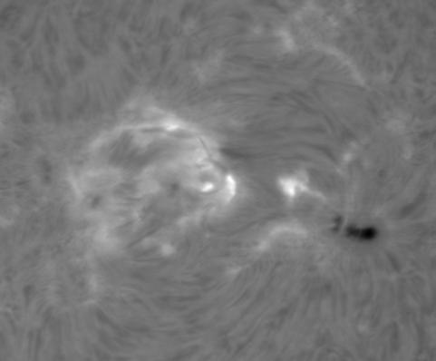
 (f) Hα 6563 Å images observed by ONSET and GONG.")

 (l) Composite images of SDO/AIA 94 Å (red) and 171 Å")


23 23 Fig. 3. Overview of the evolution of the six flares (F1 F6). Each row is for one flare. (a) (f) Hα 6563 Å images observed by ONSET and GONG. The red and blue contours show the positive and negative line-of-sight magnetic field with levels of ± 60 G, respectively. (g) (l) Composite images of SDO/AIA 94 Å (red) and 171 Å (green), corresponding to emission temperatures of 6.3 MK and 0.6 MK, respectively. The cyan contour shows the positive line-of-sight magnetic field with a level of +60 G. (m) (r) SDO/HMI vector magnetic field after removing the 180 ambiguity of the transverse field and correcting the projection effect in the Cartesian coordinate system. The yellow contour shows the positive vertical component B z with a level of +60 G. The red and blue arrows represent the direction and magnitude of the horizontal component. The size of each panel is The center of the field of view is located at [115, -95 ] in the helioprojective coordinate system, where the center of the solar disk is located at [0, 0 ].


24 Fig. 3. Continued. 24
 Full disk image of SDO/AIA 171 Å at 04:59:59 UT on January 30. Overlaid are selected magnetic field lines at a relatively high altitude in the active region.")

25 25 Fig. 4. An example of the AIA extreme ultraviolet images and 3D coronal magnetic field lines at the moment of the flux rope bifurcation. (a) Full disk image of SDO/AIA 171 Å at 04:59:59 UT on January 30. Overlaid are selected magnetic field lines at a relatively high altitude in the active region. (b) Zoomed-in view of the region corresponding to the white box in panel (a). Overlaid are selected magnetic field lines at a relatively low altitude. The cyan field lines connect regions M and W. The green and brown field lines link regions E and W. The purple field line links regions E and M. The red field lines show the twisted flux rope in region M. The white contour in the background shows the positive vertical component B z with a level of +40 G. (c) A composite image of SDO/AIA 94 Å (red) and 171 Å (green) at 04:59:59 UT on January 29. The cyan, green, and red field lines are the same as that in panel (b). The red contour delineates the hot channel.

26 26 Fig. 5. Selected 3D magnetic field lines in the corona and associated flare ribbons of the six flares (F1 F6). The coronal magnetic field is reconstructed from photospheric vector magnetic field in the Cartesian coordinate at 05:24 UT, 11:36 UT, and 19:36 UT on January 29, and 00:36 UT, 05:00 UT, and 05:36 UT on January 30, respectively. The background shows the evolution of flare ribbons at SDO/AIA 1600 Å for 30 minutes from the onset time. The cyan lines show a large dome-like structure. The green lines include two parts, a part with low field lines connecting regions E and M, and the other part with high field lines linking regions M and W. The yellow lines extending from the western positive polarity become part of the magnetic flux rope at 05:00 UT on January 30. The red lines at a low altitude connect regions M and W. The white contour in the background shows the positive vertical component B z with a level of +40 G. The field of view (FOV) is grids with a uniform pixel size of 2.
27 27 Table 2. List of null points of the six events in active region NOAA Flare Null point label X position a (Mm) Y position a (Mm) Height b (Mm) F1 Null point a Null point b F2 Null point a F3 Null point a Null point b F4 Null point a Null point b F5 Null point a Null point b Null point c F6 Null point a Null point b Null point c Null point d a The positions of X and Y are calculated from the east and south sides of the field of view, respectively. b The height of null points is measured from the Cartesian z = 0 plane of our NLFFF computational box.


28 28 Fig. 6. Magnetic field lines in the vicinity of magnetic null points for the six flares (F1 F6). The white arrows point to the positions of null points. From low to high altitudes, the null points are labeled alphabetically and their associated field lines are represented by red, cyan, yellow, and gray lines, respectively. The background shows direct comparisons between QSLs at the z = 0 layer with Q values above 10 3 (black solid lines) and the evolution of flare ribbons at SDO/AIA 1600 Å (same as the background of Figure 5).
 A snapshot of 3D QSLs viewed along a selected direction for flare F4, which is calculated from the nonlinear")


29 29 Fig. 7. QSLs in flares F4 and F5 showing the topological structures at the flux rope bifurcation. (a) A snapshot of 3D QSLs viewed along a selected direction for flare F4, which is calculated from the nonlinear force-free field. The yellow lines represent the bifurcated portion of the magnetic flux rope, while the green lines all lie within the large-scale dome-like QSL. The background image in black and white displays the SDO/HMI B z component at 00:36 UT on January 30. (b) (c) A snapshot of 3D QSLs viewed along the X-axis for flare F4. The field lines in panel (b) are the same as in panel (a). Panels (d) (f) show the same quantities as panels (a) (c), but for flare F5.


.")
.")
 A Q-map on the bottom that is calculated from the nonlinear force-free field in")
 (h) Q-map slices perpendicular to the xy plane at positions marked in panel (e).")
30 30 Fig. 8. Magnetic topology at the moment of the magnetic flux rope formation and bifurcation. (a) Bald-patch (BP) reconnection at the moment of magnetic flux rope formation. The green and red lines represent the magnetic field lines before and after magnetic reconnection, respectively. (b) Q-map slice roughly along the flux rope axis. The FOV is the same as panel (a). (c) BP reconnection at the moment of the magnetic flux rope bifurcation. The green and red lines have the same meaning as in panel (a). (d) Q-map slice roughly along the field lines. The FOV is the same as panel (c). (e) A Q-map on the bottom that is calculated from the nonlinear force-free field in the xy plane at z = 0. Overplotted are the three slices shown in panels (f) (h). (f) (h) Q-map slices perpendicular to the xy plane at positions marked in panel (e). Panel (g) shows a BP structure and panel (h) displays an HFT structure at a low height. In all panels except panel (e), the background in black and white shows the SDO/HMI B z component.
 represent flare ribbons.")
31 31 (a) - + R1 - + (b) - + R1 - + R2 1. Shear Arcades R2 2. Flux Rope (c) - + R1 - + (d) - + R1 - + R3 R3 R2 R2 3. Bifurcated Flux Rope 4. Twisted Bifurcated Flux Rope Fig. 9. Schematic picture demonstrating the formation and bifurcation of the magnetic flux rope. Green bands (R1, R2, and R3) represent flare ribbons. The warm color field lines show that the eastern positive polarity connects to the middle negative polarity. The cold color field lines display that the western positive polarity links to the middle negative polarity. The red field line is a part of the magnetic flux rope. The background includes two positive polarities and one negative polarity. (a) Shear arcades. (b) Flux rope. (c) Bifurcated flux rope. (d) Twisted bifurcated flux rope.
arxiv: v1 [astro-ph.sr] 24 Mar 2016
![arxiv: v1 [astro-ph.sr] 24 Mar 2016](/thumbs/89/99600863.jpg "arxiv: v1 [astro-ph.sr] 24 Mar 2016") Hooked flare ribbons and flux-rope related QSL footprints Jie Zhao 1, Stuart A. Gilchrist 2,3, Guillaume Aulanier 2, Brigitte Schmieder 2, Etienne Pariat 2, Hui Li 1 arxiv:1603.07563v1 [astro-ph.sr] 24
Hooked flare ribbons and flux-rope related QSL footprints Jie Zhao 1, Stuart A. Gilchrist 2,3, Guillaume Aulanier 2, Brigitte Schmieder 2, Etienne Pariat 2, Hui Li 1 arxiv:1603.07563v1 [astro-ph.sr] 24
Coronal Magnetic Field Extrapolations
 3 rd SOLAIRE School Solar Observational Data Analysis (SODAS) Coronal Magnetic Field Extrapolations Stéphane RÉGNIER University of St Andrews What I will focus on Magnetic field extrapolation of active
arxiv: v1 [astro-ph.sr] 7 Jul 2015
![arxiv: v1 [astro-ph.sr] 7 Jul 2015](/thumbs/74/70217595.jpg "arxiv: v1 [astro-ph.sr] 7 Jul 2015") arxiv:1507.01910v1 [astro-ph.sr] 7 Jul 2015 Testing a Solar Coronal Magnetic Field Extrapolation Code with the Titov Démoulin Magnetic Flux Rope Model Chaowei Jiang, Xueshang Feng SIGMA Weather Group,
arxiv:1507.01910v1 [astro-ph.sr] 7 Jul 2015 Testing a Solar Coronal Magnetic Field Extrapolation Code with the Titov Démoulin Magnetic Flux Rope Model Chaowei Jiang, Xueshang Feng SIGMA Weather Group,
Observation of An Evolving Magnetic Flux Rope Prior To and During A Solar Eruption
 arxiv:1203.4859v1 [astro-ph.sr] 22 Mar 2012 Observation of An Evolving Magnetic Flux Rope Prior To and During A Solar Eruption March 23, 2012 Jie Zhang 1,, Xin Cheng 1,2, Ming-de Ding 2 1 School of Physics,
arxiv: v1 [astro-ph.sr] 3 Nov 2018
![arxiv: v1 [astro-ph.sr] 3 Nov 2018](/thumbs/90/101195283.jpg "arxiv: v1 [astro-ph.sr] 3 Nov 2018") Generalisation of the Magnetic Field Configuration of typical and atypical Confined Flares arxiv:1811.01228v1 [astro-ph.sr] 3 Nov 2018 Navin Chandra Joshi 1,2, Xiaoshuai Zhu 3, Brigitte Schmieder 4,2,
Generalisation of the Magnetic Field Configuration of typical and atypical Confined Flares arxiv:1811.01228v1 [astro-ph.sr] 3 Nov 2018 Navin Chandra Joshi 1,2, Xiaoshuai Zhu 3, Brigitte Schmieder 4,2,
arxiv: v1 [astro-ph.sr] 28 Apr 2013
![arxiv: v1 [astro-ph.sr] 28 Apr 2013](/thumbs/96/128014024.jpg "arxiv: v1 [astro-ph.sr] 28 Apr 2013") Accepted for publication in ApJ Letters on April 28th Preprint typeset using L A TEX style emulateapj v. 08/13/06 Online-only material: animations, color figures INVESTIGATING TWO SUCCESSIVE FLUX ROPE
Accepted for publication in ApJ Letters on April 28th Preprint typeset using L A TEX style emulateapj v. 08/13/06 Online-only material: animations, color figures INVESTIGATING TWO SUCCESSIVE FLUX ROPE
arxiv: v1 [astro-ph.sr] 25 Oct 2013
![arxiv: v1 [astro-ph.sr] 25 Oct 2013](/thumbs/92/108564205.jpg "arxiv: v1 [astro-ph.sr] 25 Oct 2013") Bull. Astr. Soc. India (213) 41, 1 12 Magnetic structure of solar active region NOAA 11158 arxiv:131.6895v1 [astro-ph.sr] 25 Oct 213 P. Vemareddy 1, A. Ambastha 1 and T. Wiegelmann 2 1 Udaipur Solar Observatory,
Bull. Astr. Soc. India (213) 41, 1 12 Magnetic structure of solar active region NOAA 11158 arxiv:131.6895v1 [astro-ph.sr] 25 Oct 213 P. Vemareddy 1, A. Ambastha 1 and T. Wiegelmann 2 1 Udaipur Solar Observatory,
Magnetic twists and energy releases in solar flares
 Hinode seminar 2 September 2015 Magnetic twists and energy releases in solar flares Toshifumi Shimizu (ISAS/JAXA, Japan) 2015.9.2 Hinode seminar 1 Eruptive solar flares! General scenario Formation of magnetic
Modelling the Initiation of Solar Eruptions. Tibor Török. LESIA, Paris Observatory, France
 Modelling the Initiation of Solar Eruptions Tibor Török LESIA, Paris Observatory, France What I will not talk about: global CME models Roussev et al., 2004 Manchester et al., 2004 Tóth et al., 2007 numerical
arxiv: v1 [astro-ph.sr] 16 Dec 2013
![arxiv: v1 [astro-ph.sr] 16 Dec 2013](/thumbs/87/97224441.jpg "arxiv: v1 [astro-ph.sr] 16 Dec 2013") Nature of Prominences and Their Role in Space Weather Proceedings IAU Symposium No. 300, 2013 B. Schmieder, J.-M. Malherbe, & S. T. Wu, eds. c 2013 International Astronomical Union DOI: 10.1017/S1743921313010983
Nature of Prominences and Their Role in Space Weather Proceedings IAU Symposium No. 300, 2013 B. Schmieder, J.-M. Malherbe, & S. T. Wu, eds. c 2013 International Astronomical Union DOI: 10.1017/S1743921313010983
Evolution of Twisted Magnetic Flux Ropes Emerging into the Corona
 Evolution of Twisted Magnetic Flux Ropes Emerging into the Corona Yuhong Fan High Altitude Observatory, National Center for Atmospheric Research Collaborators: Sarah Gibson (HAO/NCAR) Ward Manchester (Univ.
arxiv: v1 [astro-ph.sr] 31 Oct 2018
![arxiv: v1 [astro-ph.sr] 31 Oct 2018](/thumbs/89/100545743.jpg "arxiv: v1 [astro-ph.sr] 31 Oct 2018") Draft version November 1, 2018 Typeset using LATEX default style in AASTeX61 SUCCESSIVE FLUX ROPE ERUPTIONS FROM δ-sunspots REGION OF NOAA 12673 AND ASSOCIATED X-CLASS ERUPTIVE FLARES ON 2017 SEPTEMBER
Draft version November 1, 2018 Typeset using LATEX default style in AASTeX61 SUCCESSIVE FLUX ROPE ERUPTIONS FROM δ-sunspots REGION OF NOAA 12673 AND ASSOCIATED X-CLASS ERUPTIVE FLARES ON 2017 SEPTEMBER
Scaling laws of free magnetic energy stored in a solar emerging flux region
 Publ. Astron. Soc. Japan 2014 66 (4), L6 (1 5) doi: 10.1093/pasj/psu049 Advance Access Publication Date: 2014 July 14 Letter L6-1 Letter Scaling laws of free magnetic energy stored in a solar emerging
arxiv: v1 [astro-ph.sr] 4 Sep 2014
![arxiv: v1 [astro-ph.sr] 4 Sep 2014](/thumbs/93/113737525.jpg "arxiv: v1 [astro-ph.sr] 4 Sep 2014") Formation of Compound Flux Rope by The Merging of Two Filament Channels, Associated Dynamics and its Stability Navin Chandra Joshi 1 arxiv:1409.1359v1 [astro-ph.sr] 4 Sep 2014 School of Space Research,
Formation of Compound Flux Rope by The Merging of Two Filament Channels, Associated Dynamics and its Stability Navin Chandra Joshi 1 arxiv:1409.1359v1 [astro-ph.sr] 4 Sep 2014 School of Space Research,
Paper Review: Block-induced Complex Structures Building the Flare-productive Solar Active Region 12673
 Paper Review: Block-induced Complex Structures Building the Flare-productive Solar Active Region 12673 Shuhong Yang, Jun Zhang, Xiaoshuai Zhu, and Qiao Song Published 2017 November 2 ApJL, 849, L21. Introduction
Observation of an evolving magnetic flux rope before and during a solar eruption
 ARTICLE Received 31 Oct 211 Accepted 16 Feb 212 Published 2 Mar 212 DOI: 1.138/ncomms1753 Observation of an evolving magnetic flux rope before and during a solar eruption Jie Zhang 1, Xin Cheng 1,2 & Ming-de
AIA DATA ANALYSIS OVERVIEW OF THE AIA INSTRUMENT
 AIA DATA ANALYSIS OVERVIEW OF THE AIA INSTRUMENT SDO SUMMER SCHOOL ~ August 2010 ~ Yunnan, China Marc DeRosa (LMSAL) ~ derosa@lmsal.com WHAT IS SDO? The goal of Solar Dynamics Observatory (SDO) is to understand:
The Role of Magnetic Topology in the Heating of Active Region Coronal Loops
 The Role of Magnetic Topology in the Heating of Active Region Coronal Loops J.-Y. Lee 1,2, Graham Barnes 2, K.D. Leka 2, Katharine K. Reeves 1, K. E. Korreck 1, L. Golub 1, and E. E. DeLuca 1 ABSTRACT
Modelling magnetic fields in the corona using nonlinear force-free fields
 Modelling magnetic fields in the corona using nonlinear force-free fields M. S. Wheatland 1 and K. D. Leka 2 1 School of Physics Sydney Institute for Astronomy The University of Sydney 2 North West Research
RECURRENT SOLAR JETS INDUCED BY A SATELLITE SPOT AND MOVING MAGNETIC FEATURES
 2015. The American Astronomical Society. All rights reserved. doi:10.1088/0004-637x/815/1/71 RECURRENT SOLAR JETS INDUCED BY A SATELLITE SPOT AND MOVING MAGNETIC FEATURES Jie Chen 1, Jiangtao Su 1, Zhiqiang
Flare Energy Release in the Low Atmosphere
 Flare Energy Release in the Low Atmosphere Alexander G. Kosovichev, Viacheslav M. Sadykov New Jersey Institute of Technology Ivan N. Sharykin, Ivan V. Zimovets Space Research Institute RAS Santiago Vargas
Using This Flip Chart
 Using This Flip Chart Sunspots are the first indicators that a storm from the Sun is a possibility. However, not all sunspots cause problems for Earth. By following the steps in this flip chart you will
arxiv: v1 [astro-ph.sr] 8 Feb 2017
![arxiv: v1 [astro-ph.sr] 8 Feb 2017](/thumbs/93/112797536.jpg "arxiv: v1 [astro-ph.sr] 8 Feb 2017") Astronomy & Astrophysics manuscript no. Zuccarello_eruptive2confined_flares c ESO 2018 vember 12, 2018 The transition from eruptive to confined flares in the same active region F. P. Zuccarello 1, 2, R.
Astronomy & Astrophysics manuscript no. Zuccarello_eruptive2confined_flares c ESO 2018 vember 12, 2018 The transition from eruptive to confined flares in the same active region F. P. Zuccarello 1, 2, R.
Application of a data-driven simulation method to the reconstruction of the coronal magnetic field
 Research in Astron. Astrophys. 2012 Vol. 12 No. 5, 563 572 http://www.raa-journal.org http://www.iop.org/journals/raa Research in Astronomy and Astrophysics Application of a data-driven simulation method
arxiv: v1 [astro-ph.sr] 17 Jun 2014
![arxiv: v1 [astro-ph.sr] 17 Jun 2014](/thumbs/82/86745937.jpg "arxiv: v1 [astro-ph.sr] 17 Jun 2014") Draft version June 18, 214 Preprint typeset using L A TEX style emulateapj v. 8/13/6 Online-only material: animations, color figures ON THE RELATIONSHIP BETWEEN A HOT-CHANNEL-LIKE SOLAR MAGNETIC FLUX ROPE
Draft version June 18, 214 Preprint typeset using L A TEX style emulateapj v. 8/13/6 Online-only material: animations, color figures ON THE RELATIONSHIP BETWEEN A HOT-CHANNEL-LIKE SOLAR MAGNETIC FLUX ROPE
Solar-B. Report from Kyoto 8-11 Nov Meeting organized by K. Shibata Kwasan and Hida Observatories of Kyoto University
 Solar-B Report from Kyoto 8-11 Nov Meeting organized by K. Shibata Kwasan and Hida Observatories of Kyoto University The mission overview Japanese mission as a follow-on to Yohkoh. Collaboration with USA
arxiv: v1 [astro-ph.sr] 19 Dec 2013
![arxiv: v1 [astro-ph.sr] 19 Dec 2013](/thumbs/94/118319013.jpg "arxiv: v1 [astro-ph.sr] 19 Dec 2013") arxiv:1312.5389v1 [astro-ph.sr] 19 Dec 2013 1 Using Coronal Loops to Reconstruct the Magnetic Field of an Active Region Before and After a Major Flare A. Malanushenko 1,2, C. J. Schrijver 2, M. L. DeRosa
arxiv:1312.5389v1 [astro-ph.sr] 19 Dec 2013 1 Using Coronal Loops to Reconstruct the Magnetic Field of an Active Region Before and After a Major Flare A. Malanushenko 1,2, C. J. Schrijver 2, M. L. DeRosa
arxiv: v1 [astro-ph.sr] 2 Jun 2017
![arxiv: v1 [astro-ph.sr] 2 Jun 2017](/thumbs/87/97102282.jpg "arxiv: v1 [astro-ph.sr] 2 Jun 2017") DRAFT VERSION APRIL 14, 2018 Preprint typeset using LATEX style emulateapj v. 12/16/11 COMPARISON OF TWO CORONAL MAGNETIC FIELD MODELS FOR RECONSTRUCTING A SIGMOIDAL SOLAR ACTIVE REGION WITH CORONAL LOOPS
DRAFT VERSION APRIL 14, 2018 Preprint typeset using LATEX style emulateapj v. 12/16/11 COMPARISON OF TWO CORONAL MAGNETIC FIELD MODELS FOR RECONSTRUCTING A SIGMOIDAL SOLAR ACTIVE REGION WITH CORONAL LOOPS
arxiv: v1 [astro-ph.sr] 31 May 2018
![arxiv: v1 [astro-ph.sr] 31 May 2018](/thumbs/95/125112242.jpg "arxiv: v1 [astro-ph.sr] 31 May 2018") New Astronomy 00 (2018) 1?? New Astronomy arxiv:1805.12314v1 [astro-ph.sr] 31 May 2018 Formation and Eruption of a Double-decker Filament Triggered by Micro-bursts and Recurrent Jets in the Filament Channel
New Astronomy 00 (2018) 1?? New Astronomy arxiv:1805.12314v1 [astro-ph.sr] 31 May 2018 Formation and Eruption of a Double-decker Filament Triggered by Micro-bursts and Recurrent Jets in the Filament Channel
Physical modeling of coronal magnetic fields and currents
 Physical modeling of coronal magnetic fields and currents Participants: E. Elkina,, B. Nikutowski,, A. Otto, J. Santos (Moscow,Lindau,, Fairbanks, São José dos Campos) Goal: Forward modeling to understand
База данных свойств вспышечных лент, основанная на наблюдениях Солнечной Динамической обсерватории
 Online Seminar 22 Feb 2017, Ioffe Institute A Database of Flare Ribbons Observed by Solar Dynamics Observatory База данных свойств вспышечных лент, основанная на наблюдениях Солнечной Динамической обсерватории
Solar eruptive phenomena
 Solar eruptive phenomena Andrei Zhukov Solar-Terrestrial Centre of Excellence SIDC, Royal Observatory of Belgium 26/01/2018 1 Eruptive solar activity Solar activity exerts continous influence on the solar
Lecture 5 CME Flux Ropes. February 1, 2017
 Lecture 5 CME Flux Ropes February 1, 2017 energy release on the Sun in a day CMEs best seen by coronagraphs LASCO C2 CMEs best seen by coronagraphs LASCO C3 The three-part white light CME Front Core Cavity
Publ. Astron. Obs. Belgrade No. 90 (2010), A CASE OF FILAMENT ACTIVE REGION INTERACTION
, A CASE OF FILAMENT ACTIVE REGION INTERACTION") Publ. Astron. Obs. Belgrade No. 90 (2010), 125-130 Contributed Paper A CASE OF FILAMENT ACTIVE REGION INTERACTION Astronomical Institute of the Romanian Academy, Str. Cuţitul de Argint 5, 040557 Bucharest,
Publ. Astron. Obs. Belgrade No. 90 (2010), 125-130 Contributed Paper A CASE OF FILAMENT ACTIVE REGION INTERACTION Astronomical Institute of the Romanian Academy, Str. Cuţitul de Argint 5, 040557 Bucharest,
Solar Flare. A solar flare is a sudden brightening of solar atmosphere (photosphere, chromosphere and corona)
") Solar Flares Solar Flare A solar flare is a sudden brightening of solar atmosphere (photosphere, chromosphere and corona) Flares release 1027-1032 ergs energy in tens of minutes. (Note: one H-bomb: 10
Solar Flares Solar Flare A solar flare is a sudden brightening of solar atmosphere (photosphere, chromosphere and corona) Flares release 1027-1032 ergs energy in tens of minutes. (Note: one H-bomb: 10
arxiv: v2 [astro-ph.sr] 6 Nov 2018
![arxiv: v2 [astro-ph.sr] 6 Nov 2018](/thumbs/89/100542428.jpg "arxiv: v2 [astro-ph.sr] 6 Nov 2018") Draft version November 7, 2018 Preprint typeset using L A TEX style AASTeX6 v. 1.0 UNRAVELING THE LINKS AMONG SYMPATHETIC ERUPTIONS Dong Wang 1,2, Rui Liu 1, Yuming Wang 1, Tingyu Gou 1, Quanhao Zhang
Draft version November 7, 2018 Preprint typeset using L A TEX style AASTeX6 v. 1.0 UNRAVELING THE LINKS AMONG SYMPATHETIC ERUPTIONS Dong Wang 1,2, Rui Liu 1, Yuming Wang 1, Tingyu Gou 1, Quanhao Zhang
Does the magnetic kink instability trigger solar energetic events? Peter Ashton & Rachel MacDonald Mentors: K.D. Leka & Graham Barnes
 Does the magnetic kink instability trigger solar energetic events? Peter Ashton & Rachel MacDonald Mentors: K.D. Leka & Graham Barnes Overview What is the kink instability? Determining twist from observables
Photospheric and chromospheric polarimetry of solar flares
 Photospheric and chromospheric polarimetry of solar flares Lucia Kleint, Fachhochschule Nordwestschweiz Alberto Sainz Dalda, Stanford University Phil Judge, HAO/NCAR Kevin Reardon, National Solar Observatory
arxiv: v1 [astro-ph.sr] 10 Nov 2018
![arxiv: v1 [astro-ph.sr] 10 Nov 2018](/thumbs/90/102662284.jpg "arxiv: v1 [astro-ph.sr] 10 Nov 2018") Astronomy & Astrophysics manuscript no. FluxRopeDrift_ms_ArXiv c ESO 2018 November 13, 2018 Drifting of the line-tied footpoints of CME flux-ropes Guillaume Aulanier 1 and Jaroslav Dudík 2 arxiv:1811.04253v1
Astronomy & Astrophysics manuscript no. FluxRopeDrift_ms_ArXiv c ESO 2018 November 13, 2018 Drifting of the line-tied footpoints of CME flux-ropes Guillaume Aulanier 1 and Jaroslav Dudík 2 arxiv:1811.04253v1
MHD Simulation of Solar Flare Current Sheet Position and Comparison with X-ray Observations in active region NOAA 10365
 Sun and Geosphere, 2013; 8(2):71-76 ISSN 1819-0839 MHD Simulation of Solar Flare Current Sheet Position and Comparison with X-ray Observations in active region NOAA 10365 A. I. Podgorny 1, I. M. Podgorny
Keywords: Sun: radio magnetic fields Sun: chromosphere Sun: corona Sun: active regions
 Estimating the coronal and chromospheric magnetic fields of solar active regions as observed with the Nobeyama Radioheliograph Compared with the Extrapolated Linear Force-Free Field A. Mouner, Abdelrazek
Multi-wavelength VLA and Spacecraft Observations of Evolving Coronal Structures Outside Flares
 Multi-Wavelength Investigations of Solar Activity Proceedings of IAU Symposium No. 223, 2004 A.V. Stepanov, E.E. Benevolenskaya & A.G. Kosovichev, eds. Multi-wavelength VLA and Spacecraft Observations
Long range magnetic couplings between solar flares and coronal mass ejections observed by SDO and STEREO
 JOURNAL OF GEOPHYSICAL RESEARCH, VOL. 116,, doi:10.1029/2010ja016224, 2011 Long range magnetic couplings between solar flares and coronal mass ejections observed by SDO and STEREO C. J. Schrijver 1 and
THE MAGNETIC SYSTEMS TRIGGERING THE M6.6 CLASS SOLAR FLARE IN NOAA ACTIVE REGION 11158
 The Astrophysical Journal, 773:128 (1pp), 213 August 2 C 213. The American Astronomical Society. All rights reserved. Printed in the U.S.A. doi:1.188/4-637x/773/2/128 THE MAGNETIC SYSTEMS TRIGGERING THE
arxiv: v1 [astro-ph.sr] 27 Jun 2015
![arxiv: v1 [astro-ph.sr] 27 Jun 2015](/thumbs/87/95691016.jpg "arxiv: v1 [astro-ph.sr] 27 Jun 2015") Extreme Ultraviolet Imaging of Three-dimensional Magnetic Reconnection in a Solar Eruption J. Q. Sun 1, X. Cheng 1, M. D. Ding 1, Y. Guo 1, E. R. Priest 2, C. E. Parnell 2, S. J. Edwards 3, J. Zhang 4,
Extreme Ultraviolet Imaging of Three-dimensional Magnetic Reconnection in a Solar Eruption J. Q. Sun 1, X. Cheng 1, M. D. Ding 1, Y. Guo 1, E. R. Priest 2, C. E. Parnell 2, S. J. Edwards 3, J. Zhang 4,
Nonlinear force-free coronal magnetic field extrapolation scheme based on the direct boundary integral formulation
 JOURNAL OF GEOPHYSICAL RESEARCH, VOL. 113,, doi:10.1029/2007ja012441, 2008 Nonlinear force-free coronal magnetic field extrapolation scheme based on the direct boundary integral formulation Han He 1,2
Temperature Reconstruction from SDO:AIA Filter Images
 Temperature Reconstruction from SDO:AIA Filter Images A report by Chris Gilbert Astrophysical and Planetary Sciences, University of Colorado Boulder ASTR 5700; Stellar Astrophysics, Spring 2016 Abstract
Coronal Holes. Detection in STEREO/EUVI and SDO/AIA data and comparison to a PFSS model. Elizabeth M. Dahlburg
 Coronal Holes Detection in STEREO/EUVI and SDO/AIA data and comparison to a PFSS model Elizabeth M. Dahlburg Montana State University Solar Physics REU 2011 August 3, 2011 Outline Background Coronal Holes
Space weather and solar-terrestrial relations
 Space weather and solar-terrestrial relations 1 Hardi Peter Kiepenheuer-Institut für Sonnenphysik Freiburg solar eclipse, 11.8.1999, Wendy Carlos and John Kern with special thanks to Bernhard Kliem, AIP,
Twist and Flare: The role of helical magnetic structures in the solar corona Sarah Gibson
 Twist and Flare: The role of helical magnetic structures in the solar corona Sarah Gibson Yuhong Fan Cristina Mandrini, George Fisher, Pascal Demoulin Sarah Gibson September 20 Coronal Mass Ejections White
Formation of current helicity and emerging magnetic flux in solar active regions
 Mon. Not. R. Astron. Soc. 326, 57±66 (2001) Formation of current helicity and emerging magnetic flux in solar active regions Hongqi Zhang w Beijing Astronomical Observatory, National Astronomical Observatories,
arxiv: v1 [astro-ph.sr] 8 Nov 2018
![arxiv: v1 [astro-ph.sr] 8 Nov 2018](/thumbs/90/101195309.jpg "arxiv: v1 [astro-ph.sr] 8 Nov 2018") Three-dimensional Magnetic Reconnection Triggering an X-class Confined Flare in Active Region 12192 Ting Li 1,2, Yijun Hou 1,2, Shuhong Yang 1,2 & Jun Zhang 1,2 arxiv:1811.332v1 [astro-ph.sr] 8 Nov 218
Three-dimensional Magnetic Reconnection Triggering an X-class Confined Flare in Active Region 12192 Ting Li 1,2, Yijun Hou 1,2, Shuhong Yang 1,2 & Jun Zhang 1,2 arxiv:1811.332v1 [astro-ph.sr] 8 Nov 218
Exploring the Role of Magnetic Reconnection in Solar Eruptive Events
 Exploring the Role of Magnetic Reconnection in Solar Eruptive Events Jiong Qiu Physics Department, Montana State University, Bozeman MT 59717-3840, USA Abstract. We summarize our recent progress in investigating
Interaction between an emerging flux region and a pre-existing fan-spine dome observed by IRIS and SDO
 ubl. Astron. Soc. Japan (25) 67 (4), 78 ( ) doi:.93/pasj/psv47 Advance Access ublication Date: 25 June 23 78- Interaction between an emerging flux region and a pre-existing fan-spine dome observed by IRIS
arxiv: v1 [astro-ph.sr] 29 Apr 2014
![arxiv: v1 [astro-ph.sr] 29 Apr 2014](/thumbs/71/65783276.jpg "arxiv: v1 [astro-ph.sr] 29 Apr 2014") Research in Astron. & Astrophys. Vol.0 (200x) No.0, 000 000 (http://www.raa-journal.org) Research in Astronomy and Astrophysics Disappearance of a coronal hole induced by a filament activation arxiv:1404.7223v1
Research in Astron. & Astrophys. Vol.0 (200x) No.0, 000 000 (http://www.raa-journal.org) Research in Astronomy and Astrophysics Disappearance of a coronal hole induced by a filament activation arxiv:1404.7223v1
Solar Magnetic Fields Jun 07 UA/NSO Summer School 1
 Solar Magnetic Fields 1 11 Jun 07 UA/NSO Summer School 1 If the sun didn't have a magnetic field, then it would be as boring a star as most astronomers think it is. -- Robert Leighton 11 Jun 07 UA/NSO
arxiv: v1 [astro-ph.sr] 28 Sep 2015
![arxiv: v1 [astro-ph.sr] 28 Sep 2015](/thumbs/94/121305814.jpg "arxiv: v1 [astro-ph.sr] 28 Sep 2015") APJ LETTERS ACCEPTED DECEMBER 12, 17 Preprint typeset using LATEX style emulateapj v. 12/16/11 A CIRCULAR-RIBBON SOLAR FLARE FOLLOWING AN ASYMMETRIC FILAMENT ERUPTION arxiv:159.8414v1 [astro-ph.sr] 28
APJ LETTERS ACCEPTED DECEMBER 12, 17 Preprint typeset using LATEX style emulateapj v. 12/16/11 A CIRCULAR-RIBBON SOLAR FLARE FOLLOWING AN ASYMMETRIC FILAMENT ERUPTION arxiv:159.8414v1 [astro-ph.sr] 28
Observations and Magnetic Field Modeling of the Solar Flare/CME Event on 2010 April 8
 Observations and Magnetic Field Modeling of the Solar Flare/CME Event on 2010 April 8 Vincent Surges 1,2, Yingna Su 2, Adriaan van Ballegooijen 2 1. INTRODUCTION The Sun consists nearly entirely of plasma,
Astronomy. Astrophysics. Multiwavelength observation of a large-scale flux rope eruption above a kinked small filament. Pankaj Kumar and Kyung-Suk Cho
 A&A 572, A83 (2014) DOI: 10.1051/0004-6361/201323269 c ESO 2014 Astronomy & Astrophysics Multiwavelength observation of a large-scale flux rope eruption above a kinked small filament Pankaj Kumar and Kyung-Suk
arxiv: v1 [astro-ph.sr] 10 Jan 2017
![arxiv: v1 [astro-ph.sr] 10 Jan 2017](/thumbs/72/67293816.jpg "arxiv: v1 [astro-ph.sr] 10 Jan 2017") Material supply and magnetic configuration of an active region filament P. Zou 1,2,3, C. Fang 1,2,3, P. F. Chen 1,2,3, K. Yang 1,2,3, Q. Hao 1,2,3, & Wenda Cao 4 arxiv:1701.02407v1 [astro-ph.sr] 10 Jan
Material supply and magnetic configuration of an active region filament P. Zou 1,2,3, C. Fang 1,2,3, P. F. Chen 1,2,3, K. Yang 1,2,3, Q. Hao 1,2,3, & Wenda Cao 4 arxiv:1701.02407v1 [astro-ph.sr] 10 Jan
Reduced MHD. Nick Murphy. Harvard-Smithsonian Center for Astrophysics. Astronomy 253: Plasma Astrophysics. February 19, 2014
 Reduced MHD Nick Murphy Harvard-Smithsonian Center for Astrophysics Astronomy 253: Plasma Astrophysics February 19, 2014 These lecture notes are largely based on Lectures in Magnetohydrodynamics by Dalton
Science with Facilities at ARIES
 Science with Facilities at ARIES Wahab Uddin Aryabhatta Research Institute of Observational Sciences(ARIES), Nainital ARIES Science Goals with ARIES Solar Observations: [1] Ground based observations of
arxiv: v1 [astro-ph.sr] 2 Sep 2013
![arxiv: v1 [astro-ph.sr] 2 Sep 2013](/thumbs/88/117784401.jpg "arxiv: v1 [astro-ph.sr] 2 Sep 2013") arxiv:1309.0417v1 [astro-ph.sr] 2 Sep 2013 ISSN 1845 8319 SIMULTANEOUS YOHKOH /SXT AND TRACE OBSERVATIONS OF SOLAR PLASMA EJECTIONS E. CHMIELEWSKA 1, M. TOMCZAK 1, T. MROZEK 1,2 1 Astronomical Institute,
arxiv:1309.0417v1 [astro-ph.sr] 2 Sep 2013 ISSN 1845 8319 SIMULTANEOUS YOHKOH /SXT AND TRACE OBSERVATIONS OF SOLAR PLASMA EJECTIONS E. CHMIELEWSKA 1, M. TOMCZAK 1, T. MROZEK 1,2 1 Astronomical Institute,
Why are flare ribbons associated with the spines of magnetic null points generically elongated?
 Solar Physics DOI: 10.1007/ - - - - Why are flare ribbons associated with the spines of magnetic null points generically elongated? David Pontin 1 Klaus Galsgaard 2 Pascal Démoulin 3 c Springer Abstract
arxiv: v1 [astro-ph.sr] 5 Jul 2015
![arxiv: v1 [astro-ph.sr] 5 Jul 2015](/thumbs/93/111534845.jpg "arxiv: v1 [astro-ph.sr] 5 Jul 2015") Formation of Magnetic Flux Ropes during Confined Flaring Well Before the Onset of a Pair of Major Coronal Mass Ejections arxiv:1507.01165v1 [astro-ph.sr] 5 Jul 2015 Georgios Chintzoglou School of Physics,
Formation of Magnetic Flux Ropes during Confined Flaring Well Before the Onset of a Pair of Major Coronal Mass Ejections arxiv:1507.01165v1 [astro-ph.sr] 5 Jul 2015 Georgios Chintzoglou School of Physics,
The kink instability of a coronal magnetic loop as a trigger mechanism for solar eruptions
 The kink instability of a coronal magnetic loop as a trigger mechanism for solar eruptions T. Török 1 and B. Kliem 2 1 School of Mathematics and Statistics, University of St. Andrews St. Andrews, Fife
Pros and Cons (Advantages and Disadvantages) of Various Magnetic Field Extrapolation Techniques
 of Various Magnetic Field Extrapolation Techniques") Pros and Cons (Advantages and Disadvantages) of Various Magnetic Field Extrapolation Techniques Marc DeRosa Lockheed Martin Solar and Astrophysics Lab SDO Summer School ~ August 2010 ~ Yunnan, China Some
Pros and Cons (Advantages and Disadvantages) of Various Magnetic Field Extrapolation Techniques Marc DeRosa Lockheed Martin Solar and Astrophysics Lab SDO Summer School ~ August 2010 ~ Yunnan, China Some
arxiv: v1 [astro-ph.sr] 4 May 2013
![arxiv: v1 [astro-ph.sr] 4 May 2013](/thumbs/84/89710775.jpg "arxiv: v1 [astro-ph.sr] 4 May 2013") Astronomy & Astrophysics manuscript no. ms c ESO 2013 May 7, 2013 Recurrent Coronal Jets Induced by Repetitively Accumulated Electric Currents Y. Guo 1,2, P. Démoulin 3, B. Schmieder 3, M. D. Ding 1,2,
Astronomy & Astrophysics manuscript no. ms c ESO 2013 May 7, 2013 Recurrent Coronal Jets Induced by Repetitively Accumulated Electric Currents Y. Guo 1,2, P. Démoulin 3, B. Schmieder 3, M. D. Ding 1,2,
Magnetic Reconnection Flux and Coronal Mass Ejection Velocity
 Magnetic Reconnection Flux and Coronal Mass Ejection Velocity Jiong Qiu 1,2,3 & Vasyl B. Yurchyshyn 1 1. Big Bear Solar Observatory, New Jersey Institute of Technology 40386 N. Shore Ln., Big Bear City,
arxiv: v1 [astro-ph.sr] 8 Jul 2017
![arxiv: v1 [astro-ph.sr] 8 Jul 2017](/thumbs/83/87091540.jpg "arxiv: v1 [astro-ph.sr] 8 Jul 2017") Elongation of Flare Ribbons Jiong Qiu 1, Dana W. Longcope 1, Paul A. Cassak 2, Eric R. Priest 3 arxiv:1707.02478v1 [astro-ph.sr] 8 Jul 2017 1. Department of Physics, Montana State University, Bozeman MT
Elongation of Flare Ribbons Jiong Qiu 1, Dana W. Longcope 1, Paul A. Cassak 2, Eric R. Priest 3 arxiv:1707.02478v1 [astro-ph.sr] 8 Jul 2017 1. Department of Physics, Montana State University, Bozeman MT
arxiv: v1 [astro-ph.sr] 12 Apr 2014
![arxiv: v1 [astro-ph.sr] 12 Apr 2014](/thumbs/89/100155094.jpg "arxiv: v1 [astro-ph.sr] 12 Apr 2014") Not to appear in Nonlearned J., 45. Magnetohydrodynamic Simulation of the X2.2 Solar Flare on 2011 February 15: I. Comparison with the Observations arxiv:1404.3257v1 [astro-ph.sr] 12 Apr 2014 S. Inoue
Not to appear in Nonlearned J., 45. Magnetohydrodynamic Simulation of the X2.2 Solar Flare on 2011 February 15: I. Comparison with the Observations arxiv:1404.3257v1 [astro-ph.sr] 12 Apr 2014 S. Inoue
Field line helicity as a tool for coronal physics
 Field line helicity as a tool for coronal physics Anthony Yeates with Gunnar Hornig (Dundee), Marcus Page (Durham) Helicity Thinkshop, Tokyo, 20-Nov-2017 What is magnetic helicity? The average pairwise
How to deal with measurement errors and lacking data in nonlinear force-free coronal magnetic field modelling? (Research Note)
") DOI: 10.1051/0004-6361/201014391 c ESO 2010 Astronomy & Astrophysics How to deal with measurement errors and data in nonlinear force-free coronal magnetic field modelling? (Research Note. Wiegelmann and.
DOI: 10.1051/0004-6361/201014391 c ESO 2010 Astronomy & Astrophysics How to deal with measurement errors and data in nonlinear force-free coronal magnetic field modelling? (Research Note. Wiegelmann and.
Solar Structure. Connections between the solar interior and solar activity. Deep roots of solar activity
 Deep roots of solar activity Michael Thompson University of Sheffield Sheffield, U.K. michael.thompson@sheffield.ac.uk With thanks to: Alexander Kosovichev, Rudi Komm, Steve Tobias Connections between
arxiv: v1 [astro-ph.sr] 18 Mar 2017
![arxiv: v1 [astro-ph.sr] 18 Mar 2017](/thumbs/72/66746903.jpg "arxiv: v1 [astro-ph.sr] 18 Mar 2017") Numerical Simulations of the Evolution of Solar Active Regions: the Complex AR12565 and AR12567 Cristiana Dumitrache Astronomical Institute of Romanian Academy, Str. Cutitul de Argint 5, 040557 Bucharest,
Numerical Simulations of the Evolution of Solar Active Regions: the Complex AR12565 and AR12567 Cristiana Dumitrache Astronomical Institute of Romanian Academy, Str. Cutitul de Argint 5, 040557 Bucharest,
Forecas(ng the Magne(c Field Configura(on of CMEs
 Volker Bothmer University of Göttingen Institute for Astrophysics 26 October 2015 ISEST Workshop, UNAM, Mexico City Forecas(ng the Magne(c Field Configura(on of CMEs Outline 1. Magnetic field configuration
MODELLING TWISTED FLUX TUBES PHILIP BRADSHAW (ASTROPHYSICS)
") MODELLING TWISTED FLUX TUBES PHILIP BRADSHAW (ASTROPHYSICS) Abstract: Twisted flux tubes are important features in the Universe and are involved in the storage and release of magnetic energy. Therefore
MODELLING TWISTED FLUX TUBES PHILIP BRADSHAW (ASTROPHYSICS) Abstract: Twisted flux tubes are important features in the Universe and are involved in the storage and release of magnetic energy. Therefore
Toward Interplanetary Space Weather: Strategies for Manned Missions to Mars
 centre for fusion, space and astrophysics Toward Interplanetary Space Weather: Strategies for Manned Missions to Mars Presented by: On behalf of: Jennifer Harris Claire Foullon, E. Verwichte, V. Nakariakov
Space Physics: Recent Advances and Near-term Challenge. Chi Wang. National Space Science Center, CAS
 Space Physics: Recent Advances and Near-term Challenge Chi Wang National Space Science Center, CAS Feb.25, 2014 Contents Significant advances from the past decade Key scientific challenges Future missions
The Structure of the Sun. CESAR s Booklet
 How stars work In order to have a stable star, the energy it emits must be the same as it can produce. There must be an equilibrium. The main source of energy of a star it is nuclear fusion, especially
TRACE DOWNFLOWS AND ENERGY RELEASE
 TRACE DOWNFLOWS AND ENERGY RELEASE Ayumi Asai (1), T. Yokoyama (2), M. Shimojo (3), R. TanDokoro (4), M. Fujimoto (4), and K. Shibata (1) (1 ) Kwasan and Hida Observatories, Kyoto University, Kyoto, 607-8471
JOURNAL OF GEOPHYSICAL RESEARCH, VOL. 110, A08104, doi: /2004ja010934, 2005
 JOURNAL OF GEOPHYSICAL RESEARCH, VOL. 110,, doi:10.1029/2004ja010934, 2005 Toward magnetic field dissipation during the 23 July 2002 solar flare measured with Solar and Heliospheric Observatory/Michelson
Observations and models of solar coronal jets
 Tuesday October 27 th 2015 12th Postdam Thinkshop Postdam, Germany Observations and models of solar coronal jets Etienne Pariat 1 LESIA, Observatoire de Paris, PSL*, CNRS, UPMC, U. Denis Diderot, France
Solar Astrophysics with ALMA. Sujin Kim KASI/EA-ARC
 Solar Astrophysics with ALMA Sujin Kim KASI/EA-ARC Contents 1. The Sun 2. ALMA science targets 3. ALMA capabilities for solar observation 4. Recent science results with ALMA 5. Summary 2 1. The Sun Dynamic
The Interior Structure of the Sun
 The Interior Structure of the Sun Data for one of many model calculations of the Sun center Temperature 1.57 10 7 K Pressure 2.34 10 16 N m -2 Density 1.53 10 5 kg m -3 Hydrogen 0.3397 Helium 0.6405 The
Can we determine the filament chirality by the filament footpoint location or the barb-bearing?
 Research in Astronomy and Astrophysics PAPER Can we determine the filament chirality by the filament footpoint location or the barb-bearing? To cite this article: Qi Hao et al 2016 Res. Astron. Astrophys.
FASR and Radio Measurements Of Coronal Magnetic Fields. Stephen White University of Maryland
 FASR and Radio Measurements Of Coronal Magnetic Fields Stephen White University of Maryland Radio Emission and the Coronal Magnetic Field The range of magnetic fields in the corona is such that electrons
Solar Physics with Radio Observations, Proceedings of Nobeyama Symposium 1998, NRO Report 479. Flare Loop Geometry. Nariaki Nitta
 Solar Physics with Radio Observations, Proceedings of Nobeyama Symposium 1998, NRO Report 479 Flare Loop Geometry Nariaki Nitta Lockheed Martin Solar and Astrophysics Laboratory O/H1-12, B/252, 3251 Hanover
arxiv: v1 [astro-ph.sr] 20 Jun 2014
![arxiv: v1 [astro-ph.sr] 20 Jun 2014](/thumbs/80/82501540.jpg "arxiv: v1 [astro-ph.sr] 20 Jun 2014") Astronomy & Astrophysics manuscript no. paper_1_aa ESO 2014 June 23, 2014 The Solar Cycle Variation of Topological Structures in the Global Solar Corona S. J. Platten 1, C. E. Parnell 1, A. L. Haynes 1,
Astronomy & Astrophysics manuscript no. paper_1_aa ESO 2014 June 23, 2014 The Solar Cycle Variation of Topological Structures in the Global Solar Corona S. J. Platten 1, C. E. Parnell 1, A. L. Haynes 1,
Astronomy. Astrophysics. Numerical modelling of 3D reconnection. II. Comparison between rotational and spinning footpoint motions
 A&A 459, 627 639 (2006) DOI: 10.1051/0004-6361:20065716 c ESO 2006 Astronomy & Astrophysics Numerical modelling of 3D reconnection II. Comparison between rotational and spinning footpoint motions I. De
Microwave and hard X-ray imaging observations of energetic electrons in solar flares: event of 2003 June 17
 Microwave and hard X-ray imaging observations of energetic electrons in solar flares: event of 2003 June 17 Kundu, M R., Schmahl, E J, and White, S M Introduction We discuss one large flare using simultaneous
Why is the Solar Corona So Hot? James A. Klimchuk Heliophysics Divison NASA Goddard Space Flight Center
 Why is the Solar Corona So Hot? James A. Klimchuk Heliophysics Divison NASA Goddard Space Flight Center Total Solar Eclipse Aug. 1, 2008 M. Druckmuller Coronal Soft X-rays Yohkoh / SXT Surface Magnetic
arxiv: v1 [astro-ph.sr] 8 Feb 2012
![arxiv: v1 [astro-ph.sr] 8 Feb 2012](/thumbs/90/104336730.jpg "arxiv: v1 [astro-ph.sr] 8 Feb 2012") Evidence for collapsing fields in corona and photosphere during the 15 February 2011 X2.2 flare: SDO AIA and HMI Observations S. Gosain 1,2 arxiv:1202.1784v1 [astro-ph.sr] 8 Feb 2012 Received sgosain@nso.edu
Evidence for collapsing fields in corona and photosphere during the 15 February 2011 X2.2 flare: SDO AIA and HMI Observations S. Gosain 1,2 arxiv:1202.1784v1 [astro-ph.sr] 8 Feb 2012 Received sgosain@nso.edu
Multi- wavelength observations of active region evolution
 UCL Department of Space and Climate Physics Mullard Space Science Laboratory Multi- wavelength observations of active region evolution Lucie Green & Lidia van Driel- Gesztelyi Active Region - Definition
Chapter 8 Geospace 1
 Chapter 8 Geospace 1 Previously Sources of the Earth's magnetic field. 2 Content Basic concepts The Sun and solar wind Near-Earth space About other planets 3 Basic concepts 4 Plasma The molecules of an
Magnetic Energy and Helicity in Two Emerging Active Regions in the Sun
 Magnetic Energy and Helicity in Two Emerging Active Regions in the Sun Y. Liu 1, P. W. Schuck 2 ABSTRACT The magnetic energy and relative magnetic helicity in two solar active regions AR 11072 and AR 11158
EFFECTS OF MAGNETIC TOPOLOGY ON CME KINEMATIC PROPERTIES
 EFFECTS OF MAGNETIC TOPOLOGY ON CME KINEMATIC PROPERTIES Wei Liu (1), Xue Pu Zhao (1), S. T. Wu (2), Philip Scherrer (1) (1) W. W. Hansen Experimental Physics Laboratory, Stanford University, Stanford,
arxiv: v1 [astro-ph.sr] 26 Jun 2012
![arxiv: v1 [astro-ph.sr] 26 Jun 2012](/thumbs/83/87242613.jpg "arxiv: v1 [astro-ph.sr] 26 Jun 2012") Research in Astron. Astrophys. 2012 Vol. XX No. XX, 000 000 http://www.raa-journal.org http://www.iop.org/journals/raa Research in Astronomy and Astrophysics arxiv:1206.5917v1 [astro-ph.sr] 26 Jun 2012
Research in Astron. Astrophys. 2012 Vol. XX No. XX, 000 000 http://www.raa-journal.org http://www.iop.org/journals/raa Research in Astronomy and Astrophysics arxiv:1206.5917v1 [astro-ph.sr] 26 Jun 2012
Evolution of the Sheared Magnetic Fields of Two X-Class Flares Observed by Hinode/XRT
 PASJ: Publ. Astron. Soc. Japan 59, S785 S791, 2007 November 30 c 2007. Astronomical Society of Japan. Evolution of the Sheared Magnetic Fields of Two X-Class Flares Observed by Hinode/XRT Yingna SU, 1,2,3
Outline of Presentation. Magnetic Carpet Small-scale photospheric magnetic field of the quiet Sun. Evolution of Magnetic Carpet 12/07/2012
 Outline of Presentation Karen Meyer 1 Duncan Mackay 1 Aad van Ballegooijen 2 Magnetic Carpet 2D Photospheric Model Non-Linear Force-Free Fields 3D Coronal Model Future Work Conclusions 1 University of