arxiv: v2 [astro-ph.ga] 9 Feb 2015

Transcription

1 Mon. Not. R. Astron. Soc., () Printed 1 February 215 (MN LATEX style file v2.2) arxiv: v2 [astro-ph.ga] 9 Feb 215 Large-scale environment of z 5.7 C iv absorption systems II. Spectroscopy of Lyman-α emitters C. Gonzalo Díaz 1, Emma V. Ryan-Weber 1, Jeff Cooke 1,Yusei Koyama 2,3, and Masami Ouchi 4,5 1 Centre for Astrophysics and Supercomputing, Swinburne University of Technology, Hawthorn, VIC 3122, Australia 2 National Astronomical Observatory of Japan, Mitaka, Tokyo , Japan 3 Institute of Space Astronomical Science, Japan Aerospace Exploration Agency, Sagamihara, Kanagawa , Japan 4 Institute for Cosmic Ray Research, The University of Tokyo, Kashiwa, Chiba , Japan 5 Kavli Institute for the Physics and Mathematics of the Universe (WPI), The University of Tokyo, Kashiwa, Chiba , Japan Accepted. Received ABSTRACT The flow of baryons to and from a galaxy, which is fundamental for galaxy formation and evolution, can be studied with galaxy-metal absorption system pairs. Our search for galaxies around C iv absorption systems at z 5.7 showed an excess of photometric Lyman-α emitter (LAE) candidates in the fields J and J Here we present spectroscopic follow-up of 33 LAEs in both fields. In the first field, three out of the five LAEs within 1h projected comoving Mpc from the C iv system are within ±5 km s from the absorption at z C iv = ±.1. The closest candidate (LAE ) is robustly confirmed at h physical kpc from the C iv system. In the second field, the LAE sample is selected at a lower redshift ( z.4) than the C iv absorption system as a result of the filter transmission and, thus, do not trace its environment. The observed properties of LAE indicate that it is near the highmass end of the LAE distribution, probably having a large H i column density and large-scale outflows. Therefore, our results suggest that the C iv system is likely produced by a star-forming galaxy which has been injecting metals into the intergalactic medium since z > 6. Thus, the C iv system is either produced by LAE , implying that outflows can enrich larger volumes at z > 6 than at z 3.5, or an undetected dwarf galaxy. In either case, C iv systems like this one trace the ionized intergalactic medium at the end of cosmic hydrogen reionization and may trace the sources of the ionizing flux density. Key words: early universe, galaxies: high redshift, galaxies: intergalactic medium, galaxies: distances and redshifts. 1 INTRODUCTION The detection of metal absorption systems depends on the ionization balance of the absorbing gas, thus we can learn about the galaxies that reionized the Universe through the Based on observations obtained at the W.M. Keck Observatory, which is operated as a scientific partnership among the California Institute of Technology, the University of California, and NASA, and was made possible by the generous financial support of the W.M. Keck Foundation. gdiaz@swin.edu.au study of the environment of metal absorption systems at the tail end of the epoch of reionization (EoR). Statistical studies of C iv absorption systems across cosmic time (e.g. Ryan-Weber et al. 29; Becker, Rauch & Sargent 29; Simcoe et al. 211; D Odorico et al. 213) suggest that some physical properties of the absorbing clouds, for example the size and the number density, are changing towards higher redshift. D Odorico et al. (213) compared the column densities of C iv, Si iv and C ii in metal absorption systems across cosmic time and concluded that, at z 5.7, C iv metal absorption systems trace less dense gas (overdensities δ 1) than at z 3 (δ 1). In addition, Díaz et al. (214, hereafter Paper I) report that two independent

2 2 Díaz et. al. lines of sight towards z 5.7 C iv absorption systems are distant from the main projected over-densities of rest-frame UV bright Lyman break galaxy (LBG) candidates, opposite to the results at z 2 3 (e.g. Adelberger et al. 25; Steidel et al. 21). Thus, it is possible that the absorbing gas at these two epochs is found in different environments on large-scales, which opens the possibility that the detection of C iv systems depends on properties that are linked to larger scales that go beyond the local density of the absorbing gas, such as the ionizing flux density background. Interestingly, at scales of 1h comoving Mpc, a projected over-density of Lyman-α emitter (LAE) candidates was found in the field J towards the C iv absorption system. Similarly in the field J , the surface density of LAE candidates within 1h comoving Mpc from the C iv system is higher than the average over the observed field of view of 8 6h comoving Mpc. If these overdensities of LAEs in the environment of C iv systems are confirmed (the aim of this paper), the association of highly ionized gas with a large scale excess of faint UV star-forming galaxies would be in agreement with the current literature where faint galaxies are found to dominate the ionizing photon budget at z 6 (e.g. Cassata et al. 211; Dressler et al. 211; Finkelstein et al. 212b; Ferrara & Loeb 213; Cai et al. 214; Fontanot et al. 214). Moreover, it would imply that high ionization metal absorption systems at the end of the EoR can trace the highly ionized intergalactic medium (IGM). At smaller scales, galaxy-metal absorption system pairs provide useful information on the distribution of metals. It has been observed that C iv absorption systems with column densities N C iv> 1 14 at z = 2 3 are related to the circumgalactic medium (CGM) of LBGs (Adelberger et al. 25; Steidel et al. 21). Moreover, in these galaxies the red-shifted Lyα emission line and the blue-shifted interstellar absorption with respect to the systemic redshift determined by nebular emission lines (e.g. Hα, Hβ and O iii), is evidence for enriched gas moving at high velocities (hundreds of km s ). These galactic outflows are commonly observed in star-forming galaxies across cosmic time (Rupke, Veilleux & Sanders 25; Weiner et al. 29; Steidel et al. 21; Coil et al. 211; Jones, Stark & Ellis 212; Bouché et al. 212; Martin et al. 212; Bradshaw et al. 213; Karman et al. 214) and represent an important source of chemical feedback widely explored in theoretical studies on the redistribution of metals from star-forming regions to the CGM and the IGM (Madau, Ferrara & Rees 21; Oppenheimer & Davé 26, 28; Cen & Chisari 211; Murray, Ménard & Thompson 211; Tescari et al. 211; Brook et al. 212; Hopkins, Quataert & Murray 212; Shen et al. 212; Pallottini et al. 214). Although it is well accepted that star-forming galaxies can produce outflows that will enrich their CGM and potentially the IGM, the abundance of metal absorption systems and the sizes of the enriched regions suggest that a significant fraction of the metals observed in the CGM and IGM at redshift z = have been produced by satellites and progenitors of the observed galaxies during an early stage of galaxy formation at redshifts above 6 (e.g. Porciani & Madau 25; Martin et al. 21). This is commonly known as pre-galactic enrichment. For example, Shen et al. (212) use a detailed cosmological hydrodynamic simulation to study the sources of metals in the CGM of a z = 3 LBG, and find that metals observed at low radii (< 3R vir) are mainly produced in the host galaxy while metals at larger radii ( > 3R vir) are mainly produced in the satellite companions. Moreover, the metals observed at > 2R vir were released at redshift z > 5. Therefore, searching for star-forming galaxies close to the highest redshift C iv absorption systems known to date is the next step in testing theories on the enrichment of the IGM. This work presents the spectroscopic observations obtained with deimos on Keck-II for the LAE photometric candidates in Paper I. The follow-up spectroscopy demonstrates that the z 5.7 LAE selection criteria is robust, in particular for bright sources in the narrow-band filter NBC iv. We report tentative evidence that the projected over-density of LAEs in the field J corresponds to an excess of sources within ±5 km s from the second C iv absorption system at z > 5.5 in the line of sight to the QSO (z C iv,b = ±.1). However, better data is needed for at least two of the sources, to confirm the nature of emission line currently detected with very low signal-tonoise. In the field J , the sample of LAEs is not at the redshift of the C iv system and therefore does not trace the environment of this absorption system. Our spectroscopic campaign confirmed the redshift of LAE whose angular separation on the sky implies a distance of h physical kpc from the absorption system C iv b, mentioned above. This is evidence that the strongest C iv system known at z > 5.5 is associated with a detectable star-forming galaxy. Considering the evidence of the high incidence of galactic outflows at high redshift (e.g. Vanzella et al. 29; Steidel et al. 21; Jones, Stark & Ellis 212; Shibuya et al. 214), it is very likely that LAE hosts some kind of outflow. Therefore, the question of interest is whether or not the carbon produced by an earlier generation of stars in the LAE could have reached the distances at which the C iv absorption system is observed. The analysis shows that the impact parameter of 212.8h physical kpc is difficult to reconcile with a typical galactic wind scenario due to the short time since the Big Bang at which the LAE-C iv system pair is observed. As a result, even if the metals were distributed by an outflow from the LAE, the mechanisms should have already been in place at a time that is consistent with the pre-galactic enrichment scenario. Moreover, it is possible that the metals in the absorbing gas were born in undetected dwarf galaxies that polluted the IGM, while the LAE only provides the ionizing radiation to maintain the triply ionized carbon. Therefore, the simplest explanation for our results is that LAE is associated with the C iv system as the source of ionizing radiation instead of the source of enrichment. The main implication is that C iv absorption systems at z 5.7 trace highly ionized IGM. This is in agreement with predictions from cosmological simulations (e.g. Oppenheimer, Davé & Finlator 29) and suggests that C iv systems in the post-reionization Universe are important sources of information about the ionization state of the IGM. This paper is organised as follows: Section 2 describes the observations, Section 3 presents the spectroscopic catalogue of LAEs and reviews the contamination in the sample, Section 4 reviews the colours and magnitudes of z 5.7

3 Environment of z 5.7 C iv absorption systems II 3 LAEs, Section 5 presents the redshift distribution of the sample and Section 6 discusses the distribution of LAEs in the environment of C iv absorption systems, both projected and in the line of sight. After that, a description of the LAE-C iv system pair in the J field is presented in Section 7. Then, the rest-frame equivalent width of the Lyα line (hereafter EW ) and the velocity shift of the Lyα maximum (hereafter v MAX) are presented in Sections 8 and 9, respectively. Finally, the origin of the C iv system in the field J is discussed in Section 1 and the conclusions are summarised in Section 11. Throughout this work we use AB magnitudes and assume a flat universe with H = 7 km s Mpc, Ω m =.3 and Ω λ =.7. 2 OBSERVATIONS AND DATA REDUCTION: DEIMOS, KECK TELESCOPE This work is based on the spectroscopic observations of z 5.7 LAE photometric candidates from Paper I. The fields of view are centred on QSOs SDSS J (z em = 6.39, RA = 1 h 3 m 27 s.1, Dec. = ) and SDSS J (z em = 6.1, RA = 11 h 37 m 17 s.73, Dec. = ) (Fan et al. 26), hereafter J and J This section describes two data sets obtained with the DEIMOS spectrograph on the Keck-II telescope: first, the main data set collected the nights of the 27th and 28th of February 212 1, and second, additional data obtained at the end of the night of the 26th of February For the observing run of 212, the seeing was in the range.55.8 arcsec FWHM during the first night and arcsec FWHM during the second night. In order to acquire spectra of high redshift galaxies and to enable the identification of many key features of low redshift contaminants, we used the OG55 order-blocking filter and the 83 line mm grating (83G), which provides wavelength coverage from 65 to 1 Å with a central wavelength λ c = 8579 Å. For a 1 arcsec slit width, the spectral resolution is FWHM = 2.5 Å (or 91.4 km s at 82 Å), which is sampled with a scale of.47 Å per pixel. The 83G grating provides sufficient resolution to identify the O ii emission doublet of galaxies at z 1.19 (λ obs 8166 Å), which are the main contaminants in z 5.7 LAE samples. In each of the two fields, three multi-slit masks were used, carefully designed with position angles that minimise the flux lost due to atmospheric dispersion. Single exposure times of 12 seconds were adopted for all the exposures but the number of exposures per mask varied due to priority and weather conditions. In particular, for the field J the number of exposures (and total exposure time) per mask was 14 (168 s), 7 (84 s) and 3 (36 s). For the field J , we acquired 12 (144 s), 9 (18 s) and 3 (36 s) exposures per mask. Therefore, the exposure time is not uniform across the LAE sample. One additional mask per field was observed in February 214 with the same instrument but lower spectral resolution and lower signal-to-noise ratio (S/N). We used the 6 line 1 Program ID: W136D 2 Program ID: N121D mm grating (6ZD) and the GG495 order-blocking filter covering the wavelength range 5 to 15 Å with a scale of.65 Å per pixel. The width of the slits was 1 arcsec resulting in a FWHM = 3.5 Å (128. km s at 82 Å). For the field J13+524, only two exposures of 8 seconds each were obtained, which provided the detection of an emission line in three LAE candidates, although with low significance. Unfortunately, the S/N is not sufficient to distinguish lower redshift contamination because companion emission lines would be undetected and the symmetry of the line cannot be determined with sufficient accuracy (see Section 3.2). Thus, the data from February 214 for the field J is presented as tentative identification and are included in the analysis with a note of caution that the spectroscopic detections cannot robustly confirm nor rule-out the high-redshift nature of the sources. In the field J , three exposures of 15 seconds (45 s) were obtained and provided sufficient S/N to measure the redshift of LAEs and to identify contaminants. Thus, the additional data on this field are included in our analysis together with the main data set. Most of the reduction process was performed in idl using the deimos pipeline software in the spec2d package (Cooper et al. 212; Newman et al. 213). The pipeline processes the flats and arcs, which are rectified into rectangular arrays, and calculates the wavelength solution of the 2D data array. Then, it applies corrections for flatfield and fringing to the science data of each slit, which are also rectified into rectangular arrays. A b-spline model of the sky is obtained for each of the individual science exposures, and subtracted from them. The residuals are then combined into an inverse variance weighted average 2D spectrum of each slit and cosmic-rays rejection is applied on individual pixels. The spec2d package does a good job, in most cases, in the spatial direction along the slit which allows for a correct curvature rectification. However, in the dispersion direction, the 2D output spectra shows a wavelength shift in different directions respect with each other. This effect is obvious in Figure 1 that shows a section of an image created by the spec2d pipeline for quality inspection ( Allslits.[name of the mask].fits ), just before the 1D spectra are extracted. The solid line rectangle highlights the sky residuals of two consecutive slits which are not aligned. In order to solve this problem, a new wavelength dispersion solution for each 1D object spectrum was obtained, using the spectrum of the sky as comparison spectrum. Standard iraf tasks (e.g. identify, refspectra and dispcor) and the high-resolution spectral atlas of night-sky emission lines from Osterbrock et al. (1996) as reference were used to calculate the correct wavelength dispersion solution and to apply it to the objects spectra. This procedure was applied to the main data set only since the wavelength dispersion of the additional lower resolution data is properly calculated by spec2d. First, the 1D spectrum of each object was boxcar extracted from the 2D spectrum output of spec2d by direct sum of the counts in pixels with constant wavelength. The variance was obtained as the direct sum of the variances (i.e. errors added in quadrature). The extraction box position was defined by visual inspection to include all the pixels that showed flux in the 2D spectrum at the position of the object. Secondly, the spectrum of the sky was extracted from the same slit and position as the object be-

4 4 Díaz et. al. 3.1 The sample Figure 1. Example of a control image from spec2d ( Allslits.xxxx.fits ) showing four consecutive slits. The image is created to check the reduction process before the 1D spectrum extraction. Two major problems can be identified. First, red dashed line rectangles show sky emission probably from other slits. The reflected light is not removed by the model of the background and produces undesired residuals in all the slits. Second, the red solid line rectangle shows that the skylines residuals of consecutive slits are not aligned, which indicates that the automatic wavelength calibration does a poor job with our data. These effects can be avoided with an additional 5 tilt to the position angle of the slits. fore the b-spline model of the background sky was removed from the data spectrum. Thirdly, we obtained a wavelength dispersion solution for the sky emission lines measured in the same CCD columns as the object (pixel columns in deimos data correspond to the dispersion direction). The typical RMS of the fit is.3.5 Å. Finally, the same wavelength solution was assigned to the object spectrum. The output of this process is the reduced 1D spectra of the 33 line emitters presented in the following section. 3 SPECTROSCOPIC CATALOGUE OF z 5.7 LAES This section presents the spectroscopic sample and summarises the possible sources of contamination. First, we present the data. Second, we comment on the contamination level and the approach adopted to remove contaminant sources. Third, we search for evidence of Active Galactic Nuclei (AGN) among the objects in the sample. The complete sample contains 33 spectra of which 28 are photometric LAE candidates and five are extra detections that were not photometrically selected due to insufficient signal-to-noise in the NBC iv band (S/N NBC iv < 5). Spectroscopic quantities and other estimates based on the spectroscopic redshift of each LAE are presented in Tables A1, A2, A3 and A4 in Appendix A. Contamination was determined based on the asymmetry of the emission lines and visual inspection of the spectra. The contamination level in the photometric sample is 1 2 per cent, based on 25 LAE candidates with reliable spectroscopy (i.e. excluding the three low resolution spectra in J13+524). Finally, no evidence of AGN (e.g. emission from N v(1241 Å), Si iv+o vi](14 Å) and N iv(1483,1487 Å)) was found in the sample. However, the search is limited by the lack of information on other wavelengths (e.g.: X-rays, sub-mm, etc.) and the high contamination of skylines in the observed wavelength range. In the J field, spectra of 17 photometric LAE candidates have been obtained. Three of the LAEs were observed using the 6ZD grating and short exposure times, thus the asymmetry of their emission line cannot be measured with sufficient precision. We opted not to include these three objects in our discussion but, for completeness, we do measure the position of the emission line and comment on them when we consider it relevant. This leaves us with 14 photometric candidates with reliable spectroscopy. In addition, four objects with S/N NBC iv < 5 were spectroscopically confirmed to have an emission line and were included in the analysis. Thus, the total sample contains 21 spectra of which 18 (14+4) have sufficient S/N for a fair assessment of the asymmetry of the line, while the three low resolution spectra are only used to measure the position of the line. The sample is presented in Figure 2, which shows the spectra and photometry snapshots on the four bands R c, i, NBC iv and z, used in the photometric selection of Paper I. In the field J , we acquired spectra of 11 photometric LAE candidates. Four of them were observed using the 6ZD grating with exposure times long enough to provide good quality spectroscopy to determine the asymmetry of the emission line. Thus, we include the low-resolution data of this field in our discussion. One additional object with S/N NBC iv < 5 was included in the analysis after the spectroscopic confirmation of an emission line. Hence, the sample in this field contains 12 spectra (11+1) which are presented in Figure 3. The objects in both Figures 2 and 3 are sorted according to the asymmetry of the emission line, decreasing from top to bottom. The ID numbers on the left hand side are for reference to Tables A1 A4 (Appendix A), which present the information on each of the candidates. Spectra obtained with the 6ZD grating are labeled as such. All the other spectra were obtained with the 83G grating. Additional objects with S/N NBC iv < 5 (i.e. not in the sample of photometric LAE candidates) are also indicated with the corresponding label. The X symbol indicates if the object does not meet the asymmetry condition for z 5.7 LAE (see Section 3.2.1) The next section presents the search for contamination from foreground sources in the sample of LAEs.

5 Environment of z 5.7 C iv absorption systems II 5 1) 2) 3) 4) 5) 6) 7) 8) R c i NB CIV z z (redshift) S/N NB <5 16.± ± ± ± ± ± ± ±1. 1) 2) 3) 4) 5) 6) 7) 8) 9) R c i NB CIV z z (redshift) ZD 6ZD 16.9± ± ± ± ± ±.8 1.9±.2 1.2±.6 5.3±2.9 9) 7.4±1.7 1) S/N NB <5 3.±.6 1) S/N NB <5 6.2±1.9 11) 6ZD, OIII.±1.3 X 11) 6.±2. 12) 6ZD 3.±2.4 X 12) 13) 14) 15) 16) S/N NB <5 5.9±.7 4.± ± ±1.9 3.±1.2 sky Wavelength (Å) Figure 3. Snapshots and spectra of the z 5.7 LAEs in the field J Similar to Figure 2, images in the left hand correspond to 6 6 arcsec snapshot boxes of R c, i, NBC iv and z bands, and the objects are arranged by decreasing weighted skewness S w,1%. Spectra obtained with the 6ZD grating are labeled. The confirmed O iii emitter is ranked #11. 17) S/N NB <5 1.1±1.1 X 18).±1.9 X ) 2) 21) 6ZD 6ZD 6ZD 3.2±4.3.±5.2.7±5.4 sky Wavelength (Å) Figure 2. Snapshots and spectra of the z 5.7 LAEs in the field J Images on the left correspond to R c, i, NBC iv and z bands, the snapshot boxes are 6 6 arcsec. In the spectra, the vertical scale is arbitrary, the peak of the emission lines are indicated with vertical dotted lines, and the 1σ error spectra are plotted with red dotted lines. The objects are arranged by decreasing weighted skewness S w,1% (defined in Section 3.2.1) which is given in the top-right corner of each spectrum. The X indicates objects with S w,1% < 3. and the bottom panel shows the sky spectrum. The 6ZD spectra are below the double-dashed line and do not have the sensitivity required for our analysis. Nevertheless, emission lines are detected in the three cases, hence we present the data for completeness.

6 6 Díaz et. al. 3.2 Contamination in the spectroscopic sample Photometric LAE candidates are selected based on an excess of flux in the NBC iv filter. This excess could result not only from Lyα at z 5.7 but also from O ii (λ3726, 3729 Å) at z , O iii (λ57 Å) at z and Hα (λ6563 Å) at z Lower redshift contaminants are removed by a broad band colour condition (e.g. (R c z ) > 1.3, Paper I) that aims to identify the flux decrement produced at λ rest < 1216 Å and λ rest < 912 Å by the absorbing neutral hydrogen in the Universe at z 5.7. However, some contamination remains, in particular among fainter emitters. This section presents the criteria adopted to remove lower redshift contaminants based on two observational characteristics of z 5.7 LAEs. First, the Lyα line at this redshift is asymmetric due to neutral hydrogen in the galaxy, the CGM and IGM close to the source (Zheng et al. 21) whilst the emission line from a lower redshift contaminant is typically symmetric (e.g. O iii and Hα), or a doublet (e.g. O ii). Secondly, if the emission is Lyα, there are no other nebular emission lines in the observed wavelength window. The presence of additional UV emission lines in a z 5.7 LAE is typically associated with an AGN. Because AGNs produce well identified emission lines such as N v, Si iv+o vi], N iv and C iv, the sole detection of any of these transitions would indicate an AGN. However, the fraction of AGNs among z 5.7 LAEs is negligible (e.g. Ouchi et al. 21). Hence, the most common cases present no emission lines other than Lyα. As a result, lower redshift contaminants can be spectroscopically identified from the presence of additional emission lines and/or from the shape (asymmetry) of the emission line Weighted skewness The Lyα emission in our sample of LAEs is affected by the neutral hydrogen content of the post-reionization Universe. The number of intervening neutral hydrogen (H i) systems increases to higher redshifts (e.g. Becker et al. 213). As a result, the net effect in the Lyα emission line is a complete absorption of the blue side. This asymmetry could be enhanced by Lyα photons emitted from the galaxy in a direction opposite to the observer, which are scattered back towards the Earth after interacting with the receding side of a galactic wind (e.g. Hansen & Oh 26; Verhamme et al. 26; Dijkstra & Wyithe 21; Verhamme et al. 214). Therefore, these photons are doppler shifted according to the speed of the wind and, by the time they reach the neutral IGM towards the observer, they have been redshifted and cannot be absorbed by the intervening neutral hydrogen. The result is a typical red tail that in the 2D spectrum can be seen like a tadpole as in the four examples of Figure 1. For this reason, the asymmetry of the high redshift Lyα emission has become the main discriminant for lower redshift interlopers (e.g. Rhoads et al. 23; Kashikawa et al. 26; Shimasaku et al. 26; Kashikawa et al. 211). In this work, we adopted the weighted skewness criteria proposed by Kashikawa et al. (26) to quantify the asymmetry of the line profile. We estimate the weighted skewness S w,1% using λ 1%,R and λ 1%,B which are the wavelengths where the flux from the emission drops to 1 per cent of the peak value on the red and blue sides, respectively. In particular, from the 18 spectroscopic detections in the field J13+524, we find 16 with a skewness S w,1% 3. which are considered LAEs and two with S w,1% < 3. which are considered contaminants. In the field J , 1 emission lines have S w,1% 3. and two have S w,1% < 3., of which one is confirmed to be O iii(λ57) by the detection of O iii(λ4959). Regarding the photometric sample (i.e. not including the S/N NBC iv < 5 objects), we report that 13 out of 14 photometric LAE candidates ( 93 per cent) and 9 out of 11 photometric LAE candidates ( 82 per cent) are spectroscopically confirmed LAEs in the fields J and J , respectively. These translates to a contamination fraction in the photometric sample of 1 2 per cent. Interestingly, the objects in both fields that do not satisfy the asymmetry criteria are among the fainter emitters. Finally, we note that the asymmetry criterion as a discriminant of lower redshift emitters is supported by the skewness measurement of an O ii emitter and an O iii emitter in our data The O ii doublet Among the possible contamination, the main sources are O ii emitters at z because the Balmer break could mimic the Lyα forest decrement at z 5.7. Fortunately, the O ii doublet has a wavelength separation of 2.8 Å (1 + z), which is 6.1 Å at z Thus, the instrument configuration used in our observations provides the spectral resolution to identify the O ii doublet if detected with sufficient S/N. For example, Figure 4 shows the 2D and 1D spectrum of a O ii emitter detected in the field J but not a photometric LAE candidate. The 1D spectrum has been smoothed with a three pixel size boxcar and the O ii doublet is clearly distinguishable. The maximum of each line was measured at λ = Å and λ = Å which correspond to z = ±.1. The skewness of the doublet is S w,1% = 3.7±.9 which indicates that the asymmetry is opposite to that of the Lyα line: the red emission line λ is brighter than the blue emission line λ Therefore, the asymmetry of the doublet is easily detected with the resolution of our observations and we are able to discriminate O ii from Lyα Additional emission lines Detection of nebular emission lines provides a robust identification of lower redshift galaxies. The spectral range covered by the data allowed us to search for other emission lines associated with O ii emitters and O iii(λ57 Å) emitters. In the first case, we looked for Ne iii, Hδ and Hγ at the corresponding wavelengths, as shown in Figure 5 (top panel). In the second case, we searched for the presence of O iii(λ4959 Å), Hβ, Hγ and Hδ, in the wavelength windows highlighted in the middle panel of Figure 5. A careful inspection of the 2D and 1D spectra resulted in the detection of an O iii emitter in the spectroscopic sample of LAE candidates in the field J The object is labeled O iii in Figure 3, and is shown in

7 Environment of z 5.7 C iv absorption systems II OII J z OII,λ S w,1% = 3.75±.93 z OII,λ 3727 = z OII,λ 3729 = λ~6.5å Wavelength (Å) Figure 4. Example of an O ii emitter at z O ii = observed with the 83G grating. The observed wavelength of the O ii doublet is in the range covered by the NBC iv filter and, therefore, is an example of a possible source of contamination. Top: Snapshot of the 2D slit spectrum in the wavelength range covered by the NBC iv filter. Middle: 1D spectrum smoothed over 3 pixels and close-up of the emission line. The doublet is clearly resolved and the continuum is below the 1σ error (red dotted line). The magenta dot-dashed line is the scaled transmission curve of the NBC iv filter. The green vertical lines enclose the wavelength range used to determine the skewness. Bottom: Sky spectrum for reference. better detail in Figure 6. The O iii(λ4959 Å) emission line is seen at λ = Å. No other emission lines were detected. Moreover, the weighted skewness of the brightest emission line (λ rest = 57 Å) is S w,1% =.7±1. which validates the asymmetry criterion. Although the 83 line mm grating provides wavelength coverage from 65 to 1 Å, the effective wavelength range observed in each slit depends on its position on the mask. Therefore, not all the spectra cover the wavelength range necessary to explore the presence of all the possible additional emission lines that would reveal the lowredshift nature of an object. Moreover, many of the possible additional emission lines that would confirm a low redshift interloper are buried in a forest of sky-lines residuals, which makes them more difficult to be detected (Figure 5). This problem is more severe for faint objects detected with low S/N. Finally, if the emission in the NBC iv filter was Hα, the wavelength coverage of the data does not reach the wavelength of the nearest strong emission lines like Hβ and O iii (Figure 5, bottom panel). Therefore, Hα cannot be identified by the presence of other emission lines. As a result, because Hα is symmetric, identification of Hα emitters at z relies mainly on the symmetry of the line. However, the spectral energy distribution is also a discriminant if continuum is detected because, for example, an Hα emitter would show continuum flux at both sides of the emission line. In summary, the abundant emission from the night sky reduces our ability to detect additional emission lines in the galaxies spectra. The O ii emitter in Figure 4 and the LAE candidate that shows clear evidence for additional emission lines (Figure 6) also have negative asymmetry line profiles. Therefore, these objects support the asymmetry criterion Flux (arbitrary units) Flux (arbitrary units) Flux (arbitrary units) OII NeIII Wavelength (Å) Hδ Hβ OIII Hγ Wavelength (Å) Hδ Hβ OIII Wavelength (Å) Figure 5. Expected wavelength of emission lines typically present in lower redshift star-forming galaxies that could be observed if the emission in the NBC iv is either O ii, O iii or Hα. The sky spectrum is shown for reference. Many of the additional lines are buried in sky emission lines which reduces our ability to identify them. Top: O ii emitters at z = The wavelength intervals of emission lines that, within the observed spectral range, are commonly associated with O ii (λ3726, 3729 Å) are labeled in the plot: Ne iii, Hδ and Hγ. Middle: O iii emitters at z = In this case, the associated emission lines that could be observed are O iii(λ4959 Å), Hβ, Hγ and Hδ. Bottom: Hα at z = The spectral range of the data does not sample the next brighter lines after Hα (i.e.: O iii and Hβ). adopted in this work to discriminate lower redshift contaminants in the LAE sample. We conclude that additional emission would confirm the low redshift nature of an object but cannot be the only criterion used to detect contamination in the sample Magnitude dependant contamination fraction Among fainter emitters, low S/N reduces the ability to resolve a doublet from a single line and to accurately measure the asymmetry of the emission. Therefore, the level of contamination is expected to increase towards fainter magnitudes. The data set used in this work seems to agree with this expectation since, first, sources brighter than NBC iv = 24.7 mag are confirmed LAEs (S w,1% 3) and, second, LAE candidates with S w,1% < 3 are fainter than NBC iv = 24.7 mag. Figure 7 shows the relation between S w,1% and two photometric quantities: NBC iv magnitude and the flux excess in NBC iv measured by the colour (i NBC iv). Blue and red circles are LAEs in the fields J and J , respectively, observed with the 83G grating. Objects observed with the 6ZD grating in the later field are represented by red squares. We do not consider observations of J obtained with this grating be- Hγ Hα

8 8 Díaz et. al OIII z OIII zoiii,λ 57=.6371±.3 S w,1% =.7±1. z OIII,λ 4959 =.6369± Wavelength (Å) Figure 6. O iii emitter in the photometric sample of LAE candidates observed with the 6ZD grating. Two emission lines are clearly detected and correspond to O iii(λ4959 Å) and O iii(λ57 Å) at z O iii.637. Top: Snapshot of the 2D slit spectrum in the wavelength range covered by the NBC iv filter. Middle: 1D spectrum smoothed over 3 pixels and close-up of the emission line at λ rest = 57 Å, which has a skewness < 3. The red dotted line is the 1σ error and the magenta dot-dashed line is the scaled transmission curve of the NBC iv filter. Bottom: Example of sky spectrum for reference. S w,1% NB CIV (mag, auto aperture) (i NB CIV ) Figure 7. Weighted skewness as a function of NBC iv magnitude and (i NBC iv) colour. Blue and red circles correspond to the fields J and J , respectively. The star symbol highlights LAE (see Section 7). Triangles are SDF LAEs (Shimasaku et al. 26). Open squares correspond to low resolution data obtained with the 6ZD grating in the field J13+524, which are presented only for completeness. The dot-dashed horizontal line is the boundary S w,1σ = 3 above which objects are considered LAEs (solid symbol). Left: NBC iv magnitude versus S w,1%. Brighter objects tend to have higher S w,1%. In particular, spectroscopic LAEs with NBC iv < 24.7 have S w,1% 3.. The two vertical lines indicate the 5σ limit magnitude in the field J (dashed line) and the field J (dotted line). Right: (i NBC iv) versus S w,1%. In this case, there is not clear correlation between the two quantities. The vertical dashed line shows the condition (i NBC iv) > used in the photometric selection criteria for LAEs in Paper I. cause the lower S/N results in skewness measurements with large errors, but for completeness we show them in the plot with black open squares. The star symbol indicates LAE at z = 5.724, which is the closest LAE to the C iv absorption system at z C iv,b = in the field J (see Section 7). Points above and below S w,1% = 3 (grey area) are represented by solid and open symbols, respectively. In the left panel, we note a trend for fainter objects to have lower skewness, with objects in both fields following the same tendency. In comparison, however, the spectroscopic sample of z 5.7 LAEs in the Subaru Deep Field (SDF, Shimasaku et al. 26), over-plotted with grey triangles in Figure 7, seems more uniformly scattered across the range of magnitudes. The spectroscopic sample of SDF LAEs includes data with different resolution (FWHM=9.5, 7.1 and 3.97 Å). Moreover, the spectral resolution of the data affects the ability to measure the line skewness, and is therefore a source of systematic error when comparing data with different resolutions, like in Figure 7. As a result, we need larger and homogeneous samples to explore the morphology of the high-redshift Lyα emission and the information behind it in a consistent way. Finally, no obvious correlation is seen between S w,1% and (i NBC iv), which are plotted in the right panel of Figure 7. Objects above the grey area (S w,1% 3) show significant scatter in (i NBC iv). This is observed in our sample and SDF LAEs, and means that robust and bright spectroscopically confirmed LAEs can show small or large narrowband flux excess, regardless of the asymmetry of the line. Below S w,1% = 3, photometric candidates can also drop-out of the i -band and reach (i NBC iv) > 2.5, in which case the colour (i NBC iv) is only a lower limit and is more than a magnitude greater than the condition (i NBC iv) > in the photometric selection criteria for LAEs of Paper I. We conclude that the current data cannot robustly confirm nor rule out the existence of a correlation between the measured asymmetry of the emission line and the narrow-band photometric properties of the source. Nevertheless, we recall that contaminants are fainter than NBC iv = 24.7 mag which is not enough to claim a correlation, but is useful to keep in mind in further analysis of the sample. 3.3 Active Galactic Nuclei in the z 5.7 LAE sample The Lyα emission can also be powered by an AGN. However, AGNs are rarely found among high redshift LAEs (e.g. Wang et al. 24; Ouchi et al. 28; Zheng et al. 21). Unfortunately, we do not have information from other wavelengths (e.g. radio, X-ray, infrared, submillimeter) nor we have information on the rest-frame optical emission lines to search for AGN activity in the z 5.7 LAE sample. Therefore, we can only explore the presence of AGNs by searching for high ionization UV emission lines produced by AGN activity. However, the wavelength range of our data does not cover the typically strong C iv emission, thus we only searched for N v, Si iv+o vi] and N iv. Moreover, N v and Si iv+o vi], which are the brighter emission lines that could have been detected in the spectral range of the data, would be in regions of the spectrum that are heavily affected by sky emission lines. This is clearly seen in Figure 8. As a result, our ability to identify AGNs is very limited. Nevertheless, after careful visual inspection of each 2D and 1D spectra, we report no evidence of AGN activity in the spectroscopic sample.

9 Environment of z 5.7 C iv absorption systems II 9 Flux (arbitrary units) Lya NV SiIV OIV] NIVa,b CIV Wavelength (Å) Figure 8. Sky spectrum and observed wavelength of typical emission lines produced in AGNs: N v, Si iv+o vi], N iv and C iv; with Lyα in the wavelength range of the NBC iv filter. The vertical dot-dashed lines correspond to the particular case of a galaxy at z 5.7. No evidence of potential emission other than Lyα was found in the spectra (2D and 1D) of confirmed LAEs, although the spectra do not cover the wavelength of the C iv emission and most of the emission lines are in regions severely affected by sky lines. 4 COLOURS AND MAGNITUDES OF z 5.7 LAES AND CONTAMINATION IN THE PHOTOMETRIC SAMPLE 4.1 Broad-band colours The Lyα emission line can affect the broad-band colours of high redshift galaxies. In Paper I, we find that the z 6 i - dropout colour criterion is not a good tracer of galaxies at z 5.7. The effect is more significant for objects with strong Lyα emission. The reason is that the i -dropout selection is based on a condition of red (i z ) colour (e.g. (i z ) > 1.3) and the Lyα emission of a galaxy at z 5.7 would increase the flux in the i -band therefore reducing the colour (i z ). The spectroscopic data clearly confirms this expectation. Figure 9 shows the position of the photometric LAE candidates (black points) in the (R c z ) versus (i z ) colour diagram. Spectroscopically confirmed LAEs are indicated with blue circles and contaminants are indicated with red crosses. Open squares are the three LAE candidates in the field J observed with the 6ZD grating. The red dashed line is the (i z ) = 1.3 colour boundary of the i - dropout selection and only 4/33 LAEs reach this condition. Interestingly, the only spectroscopically confirmed LAE that satisfies the i -dropout condition is LAE (green star symbol), which is the closest LAE to the C iv absorption system at z C iv,b = in the field J (see Section 7). The (R c z ) colours are only lower limits in the majority of the objects because they are non-detected in R c. Nevertheless, most of them are detected in i, which means that their (i z ) colours are more robust than their (R c z ) colours. For those objects that are non-detected in z, the (i z ) colours are upper limits. In particular, the rows at (R c z ) =.86 and.61 are made of objects only detected in i and NBC iv. Moreover, good agreement is found between our LAE sample and the confirmed LAEs at z 5.7 from Shimasaku et al. (26) (green open circles). This sample also shows bluer (i z ) than expected for i -dropout, since none of them have (i z ) > 1.3. The concentration of green circles around (R c z ) 1.6 and (i z ) =.4.9 corresponds to non-detections in the R c and z bands, for which these colours are lower and upper limits, respectively. Keeping in mind that the z 5.7 LAE selection is not defined in the R C z (mag) z~5.7 LAEs (Phot.) S w,1% 3. S w,1% < 3. OII emitter LAE DZ J Shimasaku et al.(26) Ly et al.(27) OIII 1 2 i z (mag) Figure 9. Broad-band (R c z ) versus (i z ) colours of the complete photometric sample of z 5.7 LAEs (black points). The contours correspond to the photometric catalogue of detections and contain 5, 9 and 97 per cent of the sources in the catalogue. The spectroscopically confirmed LAEs (S w,1% 3.) are indicated with blue circles, and the contaminants (S w,1% < 3.) are indicated with red crosses. The open star symbol highlights LAE (see Section 7). The red dashed vertical line is the (i z ) = 1.3 boundary condition for i -dropouts, the blue solid lines indicate the colour criteria for z 5.7 LBGs of Paper I. and the green dot-dashed line shows the colour selection for z 5. LBGs of Ouchi et al. (25a). Green open circles are SDF LAEs (Shimasaku et al. 26) and solid yellow circles are lower redshift emitters in SDF from Ly et al. (27). colour colour diagram of Figure 9, it is encouraging that the broad-band colours of the LAE sample agree with the expectations from the spectrophotometry of composite spectra of LBGs used to define the z 5.7 LBG selection of Paper I. The red open triangle is the O ii emitter presented in Figure 4 and is found below the colour selection window for z 5.7 LBGs (blue solid lines), in agreement with the contamination from low redshift galaxies analysed in Paper I. The colours of low redshift (z ) narrow-band emitters from Ly et al. (27) are represented by yellow solid circles. This sample contains O ii, O iii and Hα emitters, which are the dominant contamination source in LAE searches. Moreover, the sample covers a redshift range larger than that covered by the NBC iv transmission curve. Figure 9 shows that lower redshift emitters do not occupy the broad-band colour colour region of higher redshift LAEs. As a result, the discrepancy in the colour colour distribution of interlopers and spectroscopically confirmed LAEs provides a good reason to expect a low fraction of contamination among the LAE photometric candidates. 4.2 Narrow-band colours and the LAE photometric selection criteria Figure 1 presents the colour colour diagrams where the LAE colour selection criteria are defined (green dashed lines). The photometric sample of LAEs (black points) was selected from a catalogue of robust detections (S/N NBC iv 5). They can be seen to the right and to the left of the vertical dashed lines because the condition on the broadband colours of LAEs (Paper I) requires that either colour is red, or there is no detection in all three broad-bands:

10 1 Díaz et. al. 3 3 i NB CIV (mag) 2 1 OIII i NB CIV (mag) R C z (mag) R C i (mag) Figure 1. Broad-band colours and the excess in NBC iv. Symbol key is as per Figure 9. The green dashed lines show the boundaries of the LAE colour selection criteria. Objects non-detected in R c and z accumulate at (R c z )=.86 and.61 (left), and objects non-detected in R c and i accumulate at (R c i )=.31 and.39 (right). [(R c i ) >1.] [(R c z ) >1.3] [(R c < 1σ) (i < 1σ) (z < 1σ)]. We have spectroscopic confirmation (blue circles) of photometric candidates. Those that show significant NBC iv excess but are not detected in more than one broad band are found at (R c z )=.86 and.61 (left hand panel), and at (R c i )=.31 and.39 (right hand panel). We recall that the majority of the objects are non-detected in R c (see Tables A2 and A4) and therefore both (R c i ) and (R c z ) are lower limits. The LAE discussed in Section 7 (LAE , open star symbol) is one of the objects at (R c i ) =.31 which would have been missed if only one condition (R c i ) > 1. (vertical green dashed line in the right hand panel) was applied. This means that the inclusion of the colour condition (R c z ) > 1.3 (vertical green dashed line in the left hand panel) in the selection of z 5.7 LAEs is successful among objects like LAE which are non-detected in the i -band. Furthermore, we confirm five LAEs from the seven photometric candidates selected by the NBC iv excess but not detected in any broad-band, for which we have spectra with sufficient S/N (i.e. excluding the 6ZD data in the field J13+524). Figure 1 also shows z 5.7 LAEs from SDF (Shimasaku et al. 26) in green open circles. The narrow band magnitude corresponds to the filter NB816, which is similar to NBC iv. Thus, when the measured magnitudes are compared, we consider them equivalent. We note that the selection criteria of these objects were based on their (R c z ) colour and, therefore, many of them do not reach (R c i ) > 1.. Since z 5.7 LAEs are faint broad-band sources typically non-detected in R c, we find objects that are only detected in one broadband (i or z ), or non-detected in all three broad-bands, by using a flexible broad-band colour condition (based on an OR operator) in the selection criteria. Objects with S w,1% < 3. (red crosses) do not seem to occupy a defined region. The red open triangle that indicates the colours of the O ii emitter discussed in Section 3.2 is below the colour selection condition (i NBC iv) = and bluer than (R c i ) > 1.. This is in agreement with the distribution of lower redshift emitter from Ly et al. (27) i NB CIV (mag) OIII NB CIV (mag, fixed aperture) Figure 11. Colour magnitude diagram (i NBC iv) versus NBC iv. Vertical lines indicate the NBC iv 5σ limiting magnitudes in the field J (dashed) and the field J (dotted). (yellow circles), whose narrow-band magnitude corresponds to NB816. As a result, we find that lower redshift emitters have less significant narrow-band (i NBC iv) excess. The colour magnitude diagram (i NBC iv) versus NBC iv in Figure 11 shows that the O ii emitter is among other lower redshift emitters from Ly et al. (27) which can have brighter narrow-band magnitudes than the LAE sample. Moreover, it is clear that spectroscopically confirmed LAEs (including SDF LAEs) have larger (i NBC iv) colours than the contaminant population. In particular, we note that SDF LAEs and our LAE sample are evenly distributed and mixed in the colour-magnitude diagram (i NBC iv) versus NBC iv, meaning that both samples have similar brightness and colours. In summary, our results validate the colour selection criteria for z 5.7 LAEs of Paper I and suggest low contamination among bright (NBC iv < 25 mag) photometric LAE candidates.

11 Environment of z 5.7 C iv absorption systems II 11 5 SPECTROSCOPIC REDSHIFT DISTRIBUTION Figure 12 shows the wavelength distribution of the Lyα peak emission of all the detections and the NBC iv filter transmission curve for comparison. The solid line includes all the objects in both fields and the grey histogram correspond to objects with S w,1% 3.. We find that the wavelength distribution is biased towards the blue half of the filter curve. This effect as been found in all previous narrow-band selected samples of high-redshift LAEs (e.g. Shimasaku et al. 26; Ouchi et al. 28; Kashikawa et al. 211). The reason is that the flux contribution from the red side of the Lyα emission to the NBC iv magnitude decreases towards higher redshift. If the emission is bluer than the middle point of the NBC iv transmission curve (maximum throughput), the red wing of Lyα is covered by a more sensitive section of the filter and there is more rest-frame UV flux under the filter transmission curve. If the emission is redder than the middle point of the NBC iv transmission curve, there is little rest-frame UV flux included in the NBC iv magnitude, and the red wing of the Lyα is covered by a progressively less sensitive section of the filter. Considering that Lyα is a resonant transition, radiative transfer plays a very important role in the escape of Lyα photons. Cosmological hydrodynamical simulations combined with radiative transfer have shown the effect of the dynamics of the surrounding H i gas (CGM and/or IGM) in the emission line profile. For example, Zheng et al. (21) find that radiative transfer is needed to properly model frequency diffusion in which Lyα photons close to the central wavelength diffuse out to the wings of the emission line. The implication of this effect in the observed Lyα profile is clearly seen in Figure 5 of Zheng et al. (21). They show simulated observations of Lyα profiles at z 5.7 in which the emission peak is at a longer wavelength than the peak of the intrinsic profile. Moreover, the flux at the centre of the line is strongly suppressed, which results in an observed emission profile fully contained red-wards of the true line centre (e.g. Jensen et al. 213). Because we are aware that redshift estimates from the Lyα line are affected by the H i content of the near environment of the source and its kinematics, to measure the spectroscopic redshift of a z 5.7 LAE, we prefer to use the bluest pixel of the line profile with flux over the 1σ level instead of the pixel with maximum flux, which is usually adopted in the literature (e.g. Ouchi et al. 25a; Shimasaku et al. 26; Hu et al. 21). Our choice should bring our measurement in closer agreement with the true redshift of the galaxy. The bottom panel of Figure 12 shows the redshift distribution of the LAEs in each field with line-filled histograms: black lines for J and red lines for J We notice that the redshift distribution is roughly centred at z 5.7, which is lower than the redshift of the C iv absorption systems reported in the two lines of sight. The redshift of the C iv systems are indicated by the vertical lines: dot-dashed black line and dotted black line for the two C iv systems in the field J and dashed red line for the C iv system in the field J The position of the emission under the narrow-band filter transmission curve depends on the redshift of an ob- Number Number Wavelength of Lyα emission NB CIV filter All objects S w,1% 3. J J λ MAX (Å) Spectroscopic redshift distribution z CIV = z CIV = z CIV = Bin size=5km/s at z= z BLUE (redshift) Figure 12. Top: Wavelength distribution of the maximum of the emission line of all the LAE candidates in both fields (black solid histogram). The grey filed histogram corresponds to candidates with S w,1% 3 in both fields. Individual fields are shown by the black-line filled histogram (J13+524) and red-line filled histogram (J ). The vertical lines indicate the wavelength of Lyα at the redshift of the C iv absorption systems in each field, black dot-dashed and black dotted lines for the field J and red dashed for the field J Bottom: Spectroscopic redshift distribution of confirmed LAEs (S w,1% 3), as measured from the bluest pixel of the emission line with flux above the 1σ level. Histogram key is the same as the top panel. z BLUE (redshift) S w,1% NB CIV (mag, auto aperture) (i NB CIV ) Figure 13. Narrow-band photometry versus spectroscopic redshift of emission lines with S w,1% 3.. Blue and red circles correspond to the two fields J and J , respectively. LAE is highlighted with a star symbol. Grey triangles are SDF LAEs (Shimasaku et al. 26). The open squares represent the low resolution data (i.e. 6ZD grating) in the field J13+524, and although the sensitivity is not enough, if the emission is Lyα, these objects will fill the top half of the plots which are less populated. ject. We searched for potential correlation between redshift and the narrow-band magnitude and colour and find no ob-

12 12 Díaz et. al. vious trend. Figure 13 presents the redshift of the LAEs as a function of the NBC iv magnitude (MAG AUTO) and the (i NBC iv) colour (MAG APER). Red circles correspond to LAEs in the field J and are contained in the range z , as in Figure 12, showing no correlation with NBC iv. Blue circles correspond to the field J and cover a wider redshift range z Also in this case, the apparent magnitudes of the objects in the sample do not show a dependance with redshift. The horizontal lines indicate the redshift of the C iv systems using the same line style as per Figure 12. The LAE indicated with the star symbol is LAE at z = ±.1 (Section 7). The right hand panel of Figure 13 shows the spectroscopic redshift of the LAEs versus the NBC iv excess (i NBC iv). We note there seems to be a weak trend for higher redshift objects to have larger narrowband excess. However, large photometric errors and several non-detections in the i -band prevent us to reach a meaningful conclusion. Finally, we include z 5.7 LAEs from SDF and find very good agreement with the distribution of our sample. In summary, the distribution in redshift of the spectroscopic sample of LAEs is centred at z 5.7 and no strong relation is found between the redshift and the narrow-band photometry of the LAE sample. Moreover, SDF LAEs at z 5.7 show a distribution similar to our sample in the z versus NB and z versus (i NB) planes (Figure 13). 6 THE LARGE-SCALE ENVIRONMENT OF C iv ABSORPTION SYSTEMS This section presents the spatial distribution of the complete LAE photometric sample based on spectroscopic information. Figure 14 shows the projected distribution of LAEs in the fields J (left hand panel) and J (right hand panel) in comoving Mpc with respect to the C iv lines of sight, indicated by the black star and white star, respectively. Photometric LAE candidates are represented by open circles whose sizes indicate the NBC iv magnitude in the range mag, in bins of.5 mag, with smaller circles for fainter objects. Squares indicate spectroscopic confirmation of LAEs (S w,1% 3.), and although most of them are photometric candidates (circles), the few squares without a circle correspond to object that are not included in the photometric sample because the S/N in the NBC iv band is slightly below 5. These objects are included in the analysis of the density contrasts. Finally, the red crosses are contaminants (S w,1% < 3.), which are not included in the density contrast. Following the analysis in Paper I, the contours in Figure 14 correspond to constant levels of density contrast Σ LAE/ Σ LAE, where Σ LAE is the mean surface density averaged over the size of the field and Σ LAE is the surface density of LAEs obtained using 1h comoving Mpc bin size and a Gaussian smoothing kernel with FWHM = 1h comoving Mpc. Solid contours correspond to over-dense regions, dashed contours correspond to mean density regions and dotted contours correspond to under-dense regions. In the field J (left hand panel), the contours include all the photometric LAE candidates plus the spectroscopy-only LAEs. The spectroscopic campaign confirms the projected structure reported in Paper I. The line of sight to the C iv system is found in a projected over-density of LAEs of Σ LAE(1)/ Σ LAE 1.5, where the surface density within 1h comoving Mpc radius is Σ LAE(1) = gal./arcmin 2, and the mean surface density of the field is Σ LAE = gal./arcmin 2. In the field J (right hand panel), the distribution reported in Paper I is also confirmed. After removing contaminants, the surface density of the field is Σ LAE = gal./arcmin 2. Within 1h comoving Mpc the number of LAEs is so Σ LAE(1) = gal./arcmin 2. As a result, the revised density contrast increased to Σ LAE(1)/ Σ LAE Distribution of z 5.7 LAEs in the line of sight The projected distribution of LAEs shows an over-density towards each C iv line of sight. However, spectroscopic follow-up suggests that the photometric LAE sample is at a slightly lower redshift than the C iv system in the J field (Figure 12). This result is clear in Figure 15 showing the projected distance (R) versus the radial velocity ( v) to the corresponding C iv system in each field. Red solid circles and blue solid circles are spectroscopic LAEs in the field J and the field J13+524, respectively. Open squares are LAE candidates in the field J observed with the 6ZD grating (assuming that the emission is Lyα). Projected distances are measured from the position of the corresponding C iv line of sight, and radial velocities are measured respect to the C iv system at z C iv = for J LAEs and the C iv system at z C iv = for J LAEs. The LAEs in the field J are at 17.9±6h comoving Mpc in the line of sight direction ( z LAEs = 5.698±.13, v = 784.6±585.9 km s ) from the C iv system. Figure 15 shows that all the red circles are at > 1 km s from the C iv system in the field. Thus, the photometric LAE sample is not in the immediate environment of the C iv system at z = Consequently, we cannot test the idea that the C iv system is associated with LAEs with our current data. Instead it should be tested with NB photometry better centred at the wavelength of the Lyα emission at z = Nevertheless, our spectroscopic findings presented here do not negate the results based on photometry presented in Paper I because the narrow redshift range is very useful for the interpretation of the comparison of projected distributions of galaxies. In addition, no C iv system is found in the QSO s spectrum at the redshift of the LAE sample. Since the closest LAE is at 7 transverse comoving Mpc to the line of sight region without C iv, this observation does not contradict the idea that C iv systems are preferentially detected near LAEs, as supported by the result in J where an LAE-C iv system pair has been confirmed. In the field J13+524, we find that, except for one, all spectroscopically confirmed LAEs are at > 5h comoving Mpc from the C iv system in the line of sight direction ( v > 5 km s ). This LAE is represented by the green open star symbol and is at the same redshift as the high-column density C iv absorption system in the field.

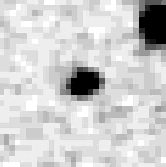
13 Environment of z 5.7 C iv absorption systems II 13 Σ LAEs /<Σ LAEs >= :31 1:3 y h (comoving Mpc) 2 2 N.5 W :4 +5:3 +5:2 Σ LAEs /<Σ LAEs >= RA (hh:mm) 11:38 11:37 11:36 y h (comoving Mpc) Projected distribution of z~5.7 LAEs N W DEC (dd:mm) +35:57 +35: x h (comoving Mpc) +5: : x h (comoving Mpc) Figure 14. Projected distribution of LAEs in the field J (left) and the field J (right). Open circles are photometric candidates and the size of each circle indicates the apparent magnitude bin with larger circles for brighter magnitudes. Open squares are confirmed by spectroscopy (S w,1% 3.) and red crosses are non-laes (S w,1% < 3.). The star symbol indicates the line of sight to the C iv systems and the the red dashed circle centred on the star symbol has a radius of 1h comoving Mpc. Masked areas of the field (bright Galactic stars and edges of the CCD) are shaded grey. The colour-coded contours correspond to constant levels of surface density contrast Σ/ Σ, obtained using 1h comoving Mpc bin size and a Gaussian smoothing kernel with FWHM of 1h comoving Mpc. Dotted contours correspond to under-dense regions (Σ/ Σ < 1), solid contours correspond to over-dense regions (Σ/ Σ > 1), and dashed contours correspond to mean density regions (Σ/ Σ = 1) Projected distance vs. peculiar velocity Rh (comoving Mpc) h (cmpc) Figure 15. Projected distance to the C iv system measured from the position of the corresponding C iv line of sight, versus radial velocity measured respect to the C iv system at z C iv = for J LAEs and the C iv system at z C iv = for J LAEs. Blue and red circles correspond to confirmed LAEs in the field J and J , respectively. The only confirmed LAE within ±5 km s (star symbol) is the closest object at 212.8h physical kpc. Open squares are LAEs observed with the 6ZD grating in J Although the data prevent a solid confirmation/rejection of these LAE candidates, we note that the position of the emission line put two of them within ±5 km s from the C iv at z C iv = This galaxy-c iv system pair is presented with more detail in the next section. The mean redshift of the sample is z LAEs = 5.72±.25 ( v = 989±1131 km s ), which shows that the sample is slightly biased towards lower redshifts. However, this value does not include the 6ZD grating data plotted as open squares. Interestingly, two of these objects are within 1h comoving Mpc of projected distance and ±5 km s of radial velocity. Although the main spectroscopic data set does not show an over-density in the line of sight direction at the position of the C iv system, if the tentative detections on the low resolution data are confirmed to be Lyα, then three out of the five LAEs within 1h projected comoving Mpc are in the near environment of the C iv absorption ( v < 5 km s ). Considering the depth sampled by the LAE selection ( 4h comoving Mpc), the confirmation of the low resolution data will imply an over-density at 1h comoving Mpc scale of (3/1)/(5/4) 2.4, where five LAEs are detected in 4h comoving Mpc depth of which three are within 1h comoving Mpc depth. In conclusion, if the emission lines in the low resolution data of the field J are found to be Lyα, it will confirm that the C iv system is associated with an excess of LAEs. 7 SPECTROSCOPIC CONFIRMATION OF AN LAE-C iv ABSORPTION SYSTEM PAIR AT z 5.7 One of the motivations to study the fields J and J is the search for galaxies physically connected to the C iv absorption systems. In this work, we report the redshift of LAE (#4 in Figure 2) to be = ±.1 measured at the position of the bluest

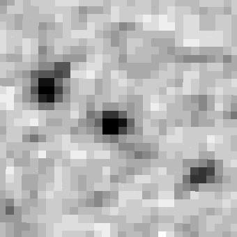
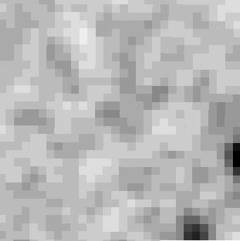
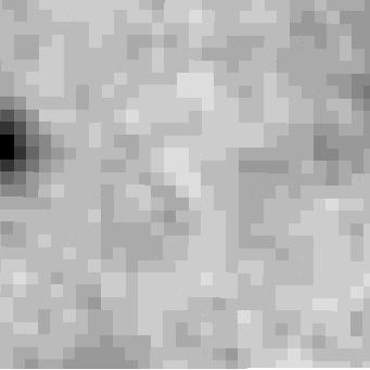
14 14 Díaz et. al. LAE Subaru, NBCIV HST ASC, F85LP (z ) P(EW,Phot. ) EW,Phot. (NB,z ) S w,1% = 11.5±1.9 z MAX = 5.727±.1 z BLUE = 5.724±.1 EW,Phot. = Å v MAX = 136±46km s blue = 2±1 1 red = 4±1 EW,Spec. = 4±31Å LAE 212.8h kpc (phys.) ~.6 arcmin Background QSO Observed wavelength (Å) v MAX = 136±46km s v(civ,b)= 9±45km s v(civ,c)= 838±45km s Figure 16. Top: Snapshot of the 2D slit spectrum in the wavelength range covered by the NBC iv filter. Middle: 1D spectrum of the emission line. The red dotted line indicates one standard deviation of the counts in the extraction box (1σ error), the magenta dot-dashed line is the scaled transmission curve of the NBC iv filter, the vertical dashed lines indicate the position of the maximum (black line) and the bluest pixel (blue line), and the grey shaded areas show the wavelength of the skylines where residuals can be large. The sky spectrum in arbitrary scale is given for reference in the bottom plot. The weighted skewness is measured in the range contained by the vertical green solid lines that indicate λ 1%,B and λ 1%,R. Inset: Equivalent width probability distribution obtained from the photometry and the redshift of the object (see Section 8). The solid line and the dashed lines indicate the central value of the distribution (33 Å) and the range enclosing a probability of.68, respectively. Bottom: Velocity with respect to the bluest pixel of the emission. The mean count level on the red side of the emission line is slightly higher than the mean value on the blue side, which is consistent with the presence of a flux decrement due to the Lyα forest. However, large errors make the values consistent with each other and with zero. The vertical solid lines indicate the wavelength range where the spectroscopic equivalent width was measured. pixel of the emission line with S/N = 1, as a proxy for the centre of the intrinsic Lyα line. This confirms that the LAE is at 212.8h physical kpc from a high column density C iv absorption system at z C iv,b = ±.1. Figure 16 presents a closer view of the spectrum of LAE The emission line shows a clear asymmetry that is quantified by a weighted skewness of S w,1% = 11.5±1.9. The vertical green solid lines (middle panel) indicate the wavelength range λ 1%,B λ 1%,R used to measure S w,1%. The maximum of the emission is indicated by the black vertical dashed line at 8178 Å, which corresponds to z MAX = 5.727±.1. However, the blue edge of the Lyα emission is very sharp whereas the red wing extends for at least 5 km s suggesting that the line centre is bluer than the observed maximum of the emission. The rest-frame equivalent width of Lyα obtained from the photometry is EW = Å, which is the lowest EW Figure 17. Top: Thumbnails (4 4 arcsec) of LAE in NBC iv with Suprime-Cam on the Subaru Telescope (left) and F85LP (z ) with ACS onboard HST (right). The black lines are the edges of the slit projected on the sky. The direction towards the background QSO is indicated with red arrows. The galaxy is distorted and elongated in the direction towards the background QSO. Middle: ACS image in the z -band showing the projected distance from LAE to the QSO line of sight. Bottom: Spectrum in km s with respect to the bluest pixel above 1σ. The vertical dashed line indicates the position of the emission peak, and the vertical dotted line and dot-dashed line show the velocity of the two C iv systems at z C iv,b = and z C iv,c = (Ryan-Weber et al. 29; Simcoe et al. 211; D Odorico et al. 213). of the LAE sample in the field J (see Section 8.2). This value is consistent with the spectroscopic measurement of EW. In the bottom panel of Figure 16, the blue squares with error bars at each side of the emission line show the mean count level of the continuum, where the vertical error bars indicate one standard deviation of the flux in counts and the horizontal error bars enclose the wavelength range used to estimate the mean. At both sides of the emission, we avoided regions of significant skyline residuals (grey areas). We measure F λ121 = 2±1 counts for the blue side of the emission, which is consistent with zero. For the red side of the emission, the flux level is F λ1225 = 4±1 counts, which is also consistent with zero. Nevertheless, we estimate EW,Spec of the observed emission within the vertical solid lines using the continuum level F λ1225 and we find EW,Spec = 4±31 Å, where the dominant source of error is the uncertainty in the continuum. The Lyα emission peak has an offset of v MAX = 136±45 km s from the redshift defined by the observed blue edge of the line. This velocity shift is smaller than the typically observed velocity offset of Lyα with respect to the systemic redshift of z 2 3 LAEs: v(lyα) = 217±29 km s (Hashimoto et al. 213). However, these two velocities are not directly comparable. On one hand, the velocity of Lyα with respect to the systemic redshift measured

15 Environment of z 5.7 C iv absorption systems II 15 from nebular emission is interpreted as evidence for gas motion in the galaxy (e.g. McLinden et al. 211; Hashimoto et al. 213). On the other hand, our measurement of v MAX is used as an indicator of the sharpness of the blue edge of the emission, meaning that smaller v MAX corresponds to line profiles with a steeper blue side. This is affected by a combination of several factors likely dominated by (a) the neutral hydrogen content in the IGM in the line of sight to the LAE, (b) H i intrinsic to the LAE, and (c) outflowing gas. Although we cannot differentiate between these effects without knowing the systemic redshift, they are probably related since galactic scale outflows can affect the distribution of the neutral gas which regulates the escape fraction of Lyα photons. Thus, although v MAX does not directly probe the speed of the outflowing gas, it is interesting to see how it compares in relation to the rest of the sample. This is discussed in Section 9. Figure 17 presents 4 4 arcsec thumbnails of LAE (top panels), showing the slit used for spectroscopy and the direction to QSO J The image in the F85LP band (which equates to z ) obtained with the Advanced Camera for Surveys (ACS) onboard the Hubble Space Telescope (right hand panel) shows a distorted shape slightly elongated towards the background QSO. The close proximity of this LAE to the line of sight of the C iv absorption systems is shown in the middle panel of the figure, and the velocity of the two C iv systems near the galaxy are shown in the bottom panel. The dot-dashed line corresponds to the second C iv absorption system at z 5.5 in this line of sight at z C iv,b = ±.1 (logn C iv = 14.52±.8, D Odorico et al. 213), with v(c iv b ) = 9 km s. The dotted line corresponds to C iv c, at z C iv,c = ±.1 (logn C iv = 13.8±.1, D Odorico et al. 213), with v(c iv c) = 838 km s. In summary, the spectroscopic redshift of LAE confirms that this galaxy is the closest neighbour to the highest column density C iv absorption system known to date at z 5.5. In addition, the red side of the emission line is very extended and reaches the wavelength corresponding to Lyα at the redshift of the C iv c absorption system. This finding demonstrates that star-forming galaxies can be detected in close proximity to highly ionized metal absorption systems immediately after the EoR, leading the path to exploring in better detail the origin and the physical state of the absorbing gas. 8 EQUIVALENT WIDTH 8.1 Measures of the Lyα emission line at z 5.7 The faint continuum of z 5.7 LAEs is the main obstacle to obtaining precise spectroscopic measurements of EW. Therefore, EW is usually measured using narrow-band and broad-band photometry (e.g: Malhotra & Rhoads 22; Hu et al. 24; Shimasaku et al. 26; Zheng et al. 214). On one hand, if the broad-band overlaps with the narrow-band (e.g. i and NBC iv), an estimate of the flux of the continuum requires the subtraction of the contribution of the Lyα emission and a correction for the IGM transmission, which are usually both unknown. On the other hand, if the broadband is redder than the narrow-band containing Lyα (e.g. z and NBC iv), then no IGM correction and no Lyα correction are needed to estimate the continuum flux. In this work, we have tested both methods and the approaches by several authors. We find that using a non-overlapping broadband tends to give stable results that are independent of the method, whereas using an overlapping broad-band is more sensitive to the corrections applied to the continuum flux density. Therefore, we adopt the EW obtained from the z and NBC iv using the following procedure. The emission line flux was estimated from the NBC iv band and the continuum flux density was measured with the z -band at λ rest 135 Å. We follow the approach suggested by Zheng et al. (214) and use the equations: N W N = a N (λ) FLyα F Lyα + b N (λ) W N EW (1 + z) (1) Z F Lyα = b Z W Z EW (1 + z), (2) where Z and N are the integrated fluxes in the z -band and the NBC iv band, respectively; and W N and W Z are the corresponding filter width W N = T N δλ/max(t N ) and W Z = T Zδλ/max(T Z), with T Z and T N representing the transmission curve of each filter. The observed Lyα flux is F Lyα and the continuum flux density was replaced by F Lyα/(EW (1 + z)). Because the narrow-band filter is not a top-hat, the contribution of the Lyα line to the NBC iv flux depends on the filter transmission at the wavelength of the emission. The coefficient a N (λ) is a correction for this effect and is estimated as the ratio of the filter transmission at the wavelength of the emission line over the maximum transmission at the centre of the filter a N = T N (λ MAX)/max(T N ). The Lyα emission is not covered by the z -band, thus the first term of equation 1 is not present in equation 2. The correction for the IGM absorption to the continuum emission in the NBC iv and z -bands is applied through b N and b Z. Since, the broad-band is redder than Lyα, no correction is necessary in z, thus b Z = 1. Considering that most of our LAEs are non-detected in R c, we assume that the contribution from the continuum bluer than Lyα (λ < λ BLUE) is negligible to flux measured by the narrow-band. Under this assumption b N is calculated as the fractional area of the NBC iv transmission curve for λ λ BLUE: b N = T λ N δλ/ T N δλ, where λ BLUE is the BLUE wavelength of the bluest pixel of the emission line. Finally, our measurements of the EW only account for the observed Lyα flux since no correction for IGM absorption to the Lyα emission was applied. In summary, our approach uses the wavelength of the emission line to estimate the corrections for individual objects. The expression for EW from equations 1 and 2 is EW,Phot. = N WZ Z bn WN 1 Z a N (1 + z). (3) The equivalent width probability function P(EW ) of each LAE was obtained by Monte Carlo simulation. Values for the z -band magnitude were pulled from a Gaussian distribution centred at the measured magnitude with a standard deviation equal to the magnitude error δz. The same process was used to sample the NBC iv magnitude, and for each pair of values we calculate EW. After 1 5 iterations, P(EW ) is obtained and from it we calculate the mean and

16 16 Díaz et. al. EW,Spec. (Å) EW,Phot. (NB, z ) (Å) Figure 18. Comparison of the spectroscopic and photometric estimates of the rest-frame equivalent width (EW ) of nine LAEs in the field J (blue circles) and five LAEs in the field J (red circles). Spectroscopy only provides upper limits for the remainder LAEs in the sample, which are not included in this figure. The dashed line is the identity relation 1:1. Points that depart from the identity towards lower spectroscopic values can result from the subtraction of sky emission lines affecting Lyα. The green star is LAE (Figure 16) and is one of the examples showing agreement in the EW measured with both methods. the errors in EW. Following Shimasaku et al. (26), the central value EW c is defined as EW c P (EW )δew =.5, and the 1σ upper and lower limits that contain 68 per cent of the distribution are estimated from EW c P (EW EW )δew =.34, and EW + EW c P (EW )δew =.34, respectively. For objects non-detected in z, lower limits in the the EW are calculated by adopting the 1σ limiting magnitude. These measurements are reported in Tables A1 and A3 in Appendix A. The equivalent width probability function of each LAE is plotted in Appendix B. In the few examples where it was possible to measure EW from the spectrum, we find that the agreement with the photometric estimates using the z magnitude for the continuum is better than using the i magnitude. Figure 18 compares the photometric and spectroscopic measurements of EW of 14 LAEs. The vertical error bars are dominated by the uncertainty in the continuum flux density. In particular, some spectra are contaminated by light from other slits (shown in Figure 1), which is a source of error for the continuum determination. Moreover, the subtraction of sky emission lines can have a significant impact in the properties of a Lyα emission line by modifying the skewness, changing the position of the emission peak and diminishing the measured line flux. Thus, it is possible that the lower values measured from the spectra of the objects below the x = y line (dashed line) are biased by these effects. Having said that, although EW,Spec have large errors, we interpret our Number This work SDF (Shimasaku et al. 26) <EW > this work = 112±75Å <EW,z > SDF = 19±59Å LAE : 33 2Å EW,Phot. (Å) Figure 19. Rest-frame equivalent width distribution of confirmed LAEs in both fields (grey filled histogram). The red line hatched histogram corresponds to SDF LAEs (Shimasaku et al. 26). The vertical lines indicate the mean value of each distribution, long-dashed for SDF LAEs and dot-dashed for our sample. The blue vertical line and line-filled region indicate EW and 1σ uncertainty of LAE , which is clearly at the low end of the distribution. results in Figure 18 as evidence that the photometric determination of EW using a non-overlapping broad-band filter returns values that are supported by spectroscopy. Nevertheless, we recognise the need for deeper spectroscopy to consistently measure the properties of z 5.7 LAEs. 8.2 Distribution of EW Figure 19 presents the EW distribution of the LAE sample of this work (grey histogram) and the LAE sample from SDF (Shimasaku et al. 26, red-dashed histogram). We find agreement in the mean and the standard deviation of both samples. The equivalent width of LAE is represented by a solid blue line and a blue-hashed region enclosing 68 per cent of the P(EW ). It is clear from this figure that LAE has a lower EW than the rest of the sample. This is interesting considering that lower redshift LAEs (z = 2 3) with lower EW values tend to display larger velocity shifts of the Lyα emission peak with respect to the systemic redshift (e.g. Hashimoto et al. 213). Moreover, the same effect is observed among LBGs (e.g. Adelberger et al. 23; Shapley et al. 23). The implications of this result are discussed in Section 1. We compare the EW with the NBC iv magnitude and (i NBC iv) colour of z 5.7 LAEs in Figure 2. Blue and red circles correspond to the samples of the present work and grey triangles correspond to SDF LAEs. In the left panel, we find no trend between EW and NBC iv magnitude since both LAE samples are well distributed across the plot. This is not a surprise because the NBC iv magnitude measures the flux of the emission line and part of the continuum while EW is a relative measure of the flux in the emission line with respect to the continuum. A rough estimate of this relation is the (i NBC iv) colour which is slightly larger for LAEs with larger EW (right panel of Figure 2). The open star symbol is LAE , and it seems to occupy a curious corner in the plot. This LAE is not detected in i, so the colour is a lower limit. Usually, other non-detections in i have larger EW because they are also very faint in z, what brings them into the relation. How-

17 Environment of z 5.7 C iv absorption systems II 17 EW,Phot. (Å) NB CIV (mag, auto aperture) (i NB CIV ) EW,Phot. (Å) 1 Figure 2. Narrow-band photometry versus EW of confirmed LAEs. Blue and red circles correspond to the two fields J and J , respectively. Triangles are SDF LAEs. LAE is highlighted with a star symbol. Left: The magnitude in NBC iv does not correlate with EW. Right: The excess (i NBC iv) shows a small trend with EW in which LAEs with higher EW have redder (i NBC iv) colour. This is also seen in the SDF sample. Considering that both quantities are independent probes of the flux excess with respect to the continuum, the existence of this relation is reasonable and encouraging. However, large uncertainties limit the detection of a significant correlation. ever, LAE is brighter in z than the other LAEs with lower-limit (i NBC iv) colours, resulting in a lower EW which is closer to the expectation for LBGs. This is clearly seen in Figure 21 which presents M UV versus EW. Symbol key is the same as per previous figures. The open star representing LAE is in the middle-bottom of the distribution and seems to agree with the trend previously noted by many authors that fainter UV galaxies at z = 5 6 have larger EW (Ando et al. 26; Shimasaku et al. 26; Stanway et al. 27; Ouchi et al. 28). The remaining LAEs with lower-limit (i NBC iv) colours are at the top-right corner of the Figure, that corresponds to large EW and faint M UV. The horizontal dotted line shows that only one LAE in our sample has a lower EW than LAE In summary, the distribution of EW is comparable with the sample of z 5.7 LAEs from SDF, and the closest neighbour to C iv b (LAE ) has one of the lowest EW, which is well determined by photometry and spectroscopy M UV (mag, 2" aperture) Figure 21. Absolute magnitude at λ rest 135 Å and EW of confirmed LAEs. As in previous figures, blue and red circles correspond to the fields J and J , respectively, and triangles are SDF LAEs. Both samples seem to follow the same relation where more luminous objects tend to have smaller EW. LAE is highlighted with a star symbol and the dotted lines (vertical and horizontal) show that fainter LAEs (i.e. to the right of LAE ) have larger EW (i.e. above LAE ). 9 VELOCITY OF THE Lyα EMISSION PEAK Many authors have found that the wavelength of the Lyα emission peak tends to be shifted from the systemic redshift of a galaxy, which is measured from nebular emission lines (Adelberger et al. 23; Steidel et al. 21; Finkelstein et al. 211; McLinden et al. 211; Hashimoto et al. 213; Chonis et al. 213; Shibuya et al. 214). The velocity shift of the Lyα emission is interpreted as the result of the dynamics of the gas. In this study, we have no measurements of the systemic redshift from rest frame optical nebular lines, thus we have adopted the redshift of the bluest pixel of the Lyα emission as the best approximation to the real redshift of the galaxy. This section presents v MAX, which is the velocity of the pixel with the maximum flux with respect to the redshift of the galaxy, and shows how it compares with other observables of LAEs such as the asymmetry of the emission line profile, the equivalent width and the UV luminosity. Starting with the distribution of v MAX, the top panel of Figure 22 shows that the mean velocity of the LAE sample is v MAX = 118±56 km s. The velocity shift measured in LAE is v MAX= 136±45 km s which is higher than the mean of the sample but within one standard deviation. The rest of the section is dedicated to the possible dependancies of v MAX with other observables plotted in Figure 22. The symbol key is the same we have used before, with the green star symbol representing LAE The errors in v MAX are very conservative since they are determined from the resolution of the obser-

18 18 Díaz et. al. vations (FWHM= 2.5 Å for the 83G data and 3.5 Å for the 6ZD data, Section 2). The second panel from the top presents v MAX versus redshift and no correlation is seen. This is not surprising since the factors that regulate the Lyα profile (e.g. speed of the gas, column density of the neutral gas, etc.) are not expected to evolve dramatically in the small redshift range of the LAE sample ( 2 Myr). Moreover, if there was a trend with redshift it would suggest that v MAX is not dominated by gas dynamics but by some observational systematic effect, which is not the case. The resonant nature of Lyα implies that radiative transfer effects coupled with the dynamics of the gas result in spatial and wavelength diffusion of Lyα photons (Hansen & Oh 26; Zheng et al. 21; Dijkstra & Kramer 212; Jeeson- Daniel et al. 212). In general, red-shifted Lyα photons find it easier to reach the observer than blue-shifted Lyα photons because they are not absorbed by the H i in the direction to the observer whereas the latter do. Furthermore, if the gas has an additional velocity component caused by some type of outflow mechanism, the Lyα photons reprocessed in the receding side of the outflow will also experience an additional redshift that will take them out of resonance allowing them to reach the observer (Ahn, Lee & Lee 23; Verhamme et al. 26; Dijkstra & Wyithe 21). In this case, the observed line profile presents a red tail that may also show some structure or bumps which increases its asymmetry. However, at fixed outflow velocities, larger H i column densities produce broader Lyα profiles and larger velocity shifts of the Lyα peak (e.g. Figure 1 of Verhamme et al. 214) which would reduce the asymmetry of the line profile. In the middle panel of Figure 22 (labeled C), there is a weak suggestion that the weighted skewness defined in Section 3.2 increases with v MAX. Considering that S w,1% measures the asymmetry of the line profile, this observable increases for a more extended red wing and sharper blue edge. Because v MAX is a measurement of the extent of the blue edge of the emission, a smaller v MAX correspond to a sharper blue edge. Therefore, a smaller v MAX should result in a more asymmetric profile, i.e. larger S w,1%. However, the opposite relation is observed since S w,1% increases with v MAX. This could indicate that the extension of the red wing may correlate, although slightly, with the shift of the Lyα peak to longer wavelengths. As mentioned before, since outflowing gas would enhance the extension of the red wing of the emission, then a galactic wind would increase S w,1% with respect to the case without it. In addition, larger H i column densities produce greater redward shifts of the Lyα peak, although reducing the asymmetry of the profile. The tentative trend in panel (C) indicates that larger H i column densities (larger v MAX) might also host stronger galactic outflows (larger S w,1% ). Under this picture, since LAE has a large v MAX and one of the a largest weighted skewness of the sample, it is possible that this galaxy contains a stronger outflow and a larger H i column density compared to the rest of the LAE sample. Panel D shows v MAX versus EW where LAE is among the lowest EW and the highest v MAX. This is in agreement with lower redshift observations that LAEs and LBGs with higher EW tend to have lower Lyα velocity shifts (e.g. Shapley et al. 23; Shibuya et z BLUE (redshift) Number S w,1% EW,Phot. (Å) M UV (mag) A < v MAX >=118±56km s LAE v MAX =136±45 km s v MAX (km s ) B C D E v MAX (km s ) Figure 22. The velocity of the Lyα emission maximum is plotted against other properties. The errors in v MAX are conservatively large as they were estimated from the FWHM of the data in the dispersion direction ( Å). Blue and red circles correspond to the fields J and J , respectively, and LAE is highlighted with a star symbol. (A) Distribution of v MAX including both fields. The complete sample of candidates is plotted with the solid line histogram and the sample of confirmed LAEs is plotted with a grey filled histogram. The dotted vertical line is LAE and is found in the high velocity half of the distribution. (B) v MAX versus redshift shows no correlation. (C) v MAX versus S w,1%. A small trend might be present in which high skewness LAEs have larger v MAX than low skewness LAEs. (D) v MAX versus EW shows that LAE has one of the lowest EW and is among the highest v MAX. (E) v MAX versus M UV shows that LAE is close to M UV (z = 6.) (horizontal dashed line) and galaxies with higher v MAX have similar M UV.

19 Environment of z 5.7 C iv absorption systems II 19 al. 214). However, the scatter shown by our data prevents us from identifying any trend. Finally, the bottom plot (panel E) presents M UV versus v MAX and shows that the galaxies with the largest v MAX values have similar M UV to LAE and close to (or larger than) M UV ( 2.24 ±.19 mag, Bouwens et al. 27, horizontal dashed line). Once again, this result is in agreement with statistics of outflows in lower redshift galaxies which have found larger wind speed in more massive galaxies (e.g. Martin 25; Weiner et al. 29; Bradshaw et al. 213). Furthermore, LAEs at z 2 3 show smaller velocity offset than bright LBGs (McLinden et al. 211, 214; Chonis et al. 213; Hashimoto et al. 213; Shibuya et al. 214). Interestingly, if more massive star-forming galaxies at z 5.7 contain larger H i column densities, then it is logical to expect that, statistically, UV brighter galaxies (i.e. more massive) have larger v MAX, lower EW and stronger outflows which result in more asymmetric profiles (larger S w,1% ). In summary, LAE presents one of the largest values of v MAX in the spectroscopic sample of LAEs. Although v MAX is not a direct measure of the outflow speed and the errors in v MAX are rather large, the tentative detection of trends with S w,1%, EW and M UV could reflect a dependence with the gas dynamics and/or the mass of the galaxy. As a result, the position of LAE in the plots of Figure 22 suggest that this LAE is a good candidate to host galactic-scale outflows among the LAEs in the sample. 1 THE ORIGIN OF C iv ABSORPTION SYSTEMS AFTER THE EPOCH OF REIONIZATION In this section we discuss the possibility that C iv b is physically associated with LAE The proximity in redshift confirms that these two object are close neighbours, thus the final question explored in this work is the possibility that the galactic scale wind of LAE enriched its environment out to > 212h physical kpc. 1.1 Evidence from the Lyα emission The distribution and kinematics of the gas in a galaxy affects the escape of Lyα photons from the galaxy and the Lyα line profile (Hansen & Oh 26; Verhamme et al. 26, 28; Dijkstra & Wyithe 21; Zheng et al. 21; Orsi, Lacey & Baugh 212; Garel et al. 212; Behrens, Dijkstra & Niemeyer 214). In Figure 17, the two C iv absorption systems at 212h projected kpc show small velocities with respect to the Lyα emission line of LAE The strongest C iv system known at z 5.5, C iv b, has a column density logn C iv= 14.52±.8 and is found at 9 km s from the LAE. The other C iv absorption system at a similar redshift, C iv c, is weaker (logn C iv= 13.8±.1) and is found at 838 km s from the LAE, which is not too far from the red end of the Lyα emission. The Lyα peak of LAE is at v MAX = 136±45 km s. Moreover, it has one of the lowest EW values (Section 8) and one of the highest v MAX values (Section 9) of the sample of LAEs in this study, which is in agreement with the observed anti-correlation between EW and v Lyα in star-forming galaxies like LBGs and LAEs at z 2 3 (e.g. Shapley et al. 23; Hashimoto et al. 213; Shibuya et al. 214). In other words: larger velocity shifts are found among lower EW. Radiative transfer studies (e.g. Verhamme et al. 28, 214) show that a higher neutral hydrogen column density results in a larger velocity shift of the Lyα peak. This is valid for outflow velocities < 3 km s since larger velocities will allow Lyα photons to escape more easily closer to the line centre, thereby reducing v Lyα. Therefore, a low v Lyα could result from a low column density of H i or a large outflow speed, whereas a large v Lyα implies not only larger H i column densities but also lower outflow speeds. This result is in agreement with Zheng et al. (21) who find the radiative transfer of Lyα photons to be dominated by the density and velocity structures of the gas in the CGM and IGM. As a result, the wavelength of the Lyα peak tends to shift to longer wavelengths in more massive dark matter haloes. Given that more luminous galaxies at z 5.7 are more massive (González et al. 211; McLure et al. 211), the trend for UV brighter LAEs to have larger v MAX shown in the bottom panel of Figure 22 is consistent with this picture. Therefore, according to the UV luminosity, Lyα profile, v MAX and EW, it is possible that LAE is at the high mass end of the LAEs, has a large H i column density, and is a good candidate for a large scale outflow. 1.2 The outflow scenario Although the speed of the outflowing gas cannot be measured without the detection of nebular emission lines and ISM absorption lines in the continuum of the galaxy, the distance to the absorption system and the limit imposed by the age of the Universe can help us to understand the origin of the metals. The separation of the LAE-C iv system is estimated from the angular separation on the sky (δθ = arcsec) and the corresponding redshifts as d = DA 2 (zlyα, z C iv,b) + (δθd M/(1 + z C iv,b )) 2, where D A(, z C iv,b ) is the angular diameter distance between the redshifts of the LAE and the C iv system and δθd M is the transverse comoving distance at the redshift of the C iv system. Figure 23 shows a diagram of the distance in the LAE-C iv system pair assuming the redshift z BLUE and z MAX and their uncertainties. The Figure clearly shows that the distance estimated from z BLUE is close to the minimum distance, which is important when considering the time needed for an outflow to reach the position of the C iv system. The time required for outflowing gas to reach a distance of 212.8h kpc depends on the speed of the gas: a typical outflow speed of 2 km s would require a time longer than the age of the Universe at z = Therefore, if the carbon was produced in stars of LAE , the outflowing material had to have a larger mean velocity during its journey. For example, at 4 km s it would have taken.518 Gyr to travel 212h kpc, implying that the outflow mechanisms were in place by z 1.1. Figure 24 presents the time required for an outflow travelling at mean velocity V outflow to reach 212.8h physical kpc (solid line) and 282h physical kpc (dotted line) corresponding to the separation determined using = z BLUE

20 2 Díaz et. al. D A12 h (physical kpc) CIV,b Distance LAE CIV system d BLUE = h kpc d MAX = h kpc 39 d MAX d BLUE z MAX LAE z BLUE z (redshift) δθd M /(1+z CIV,b ) h (physical kpc) Figure 23. Distance from C iv,b to LAE The x axis is the transverse distance δθd M /(1 + z C iv,b ) where δθ = arcsec is the angular separation on the sky. The y axis is the angular diameter distance D A between and z C iv,b. The black open circle corresponds to = z MAX and the blue solid circle corresponds to = z BLUE. The uncertainty on z C iv,b is an order of magnitude better than that of the LAE. and = z MAX, respectively. The age of the Universe at z = (.97 Gyr) provides a hard limit for the mean outflow speed. However, theoretical studies predict that the formation of the first mini-haloes capable of hosting PopIII star-formation started around 2 < z < 3 (e.g. Barkana & Loeb 21; Yoshida et al. 23; Gao et al. 27; Bromm & Yoshida 211). Moreover, the first systems that can be considered galaxies are predicted to have formed around 1 < z < 2 (e.g. Loeb 21; Greif et al. 21; Bromm & Yoshida 211). These limits imply that it is practically impossible for a low speed outflow ( V outflow < 25 km s ) from LAE to reach the position of the C iv absorption system. Mean outflow velocities in the range 25 4 km s should have departed from the LAE during the assembly of the first stars and galaxies. Finally, a strong outflow ( V outflow > 4 km s ) would have had enough time to enrich the region if the outflow was active since z 1. If the redshift of the galaxy is z MAX, then the distance to the C iv system is 282h physical kpc and stronger winds (additional 15 km s in the given examples) are required to reach the position of the C iv, which will make the lateoutflow scenario even less plausible. A comparison with outflow velocities from the literature is shown in Figure 24. Verhamme et al. (26) used 3D radiation transfer of Lyα photons and report that a model of an expanding shell of cold gas would produce a Lyα peak with a velocity shift of 2 V outflow, where V outflow is measured from the blueshift of inter-stellar absorption lines (IS). Under the assumption that v MAX is the velocity shift of the Lyα peak with respect to the systemic redshift, the outflow speed would be v MAX 68 km s (magenta shaded area), 2 which is too slow to enrich a radius of 212.8h kpc. However, this model is relevant for a single velocity shell and does not account for the full range of velocities observed in high-resolution spectra of the absorbing gas on z 2 3 star-forming galaxies. Cosmological simulations that reproduce observables t h (Gyr) Outflow travel time Big Bang First Stars First Galaxies <V> outflow (km s ) 212.8h kpc 282 h kpc.5 v MAX (Verhamme et al.26) V wind (Oppenheimer et al.29) Redshift v IS (Steidel et al.21) v IS (Shibuya et al.214) v CIV,SIV (Karman et al.214) Figure 24. Travel time versus mean outflow velocity. The solid line and the dotted line indicate the time required to travel 212.8h and 282h physical kpc, respectively. The grey horizontal areas indicate the Big Bang, the time of formation of the first mini-halos to form stars, and the time of formation of the first galaxies. Vertical colour-coded regions represent observed and predicted outflow speeds from the literature. like the comoving density of C iv ions in the IGM and the luminosity function of galaxies suggest that, among intergalactic metals, C iv is one of the best tracer of diffuse IGM in the redshift range z = 5 6 and predict that star-forming galaxies in 1 < 9 M haloes pollute the IGM for the first time and provide the flux to maintain the ionization level of the systems up to 2 physical kpc (Oppenheimer, Davé & Finlator 29). Moreover, the work of Oppenheimer, Davé & Finlator (29) suggests that C iv absorption systems with column densities in the range cm 2 are probably associated with galaxies of luminosities L L. Their best outflow model predicts mean outflow velocities between 2 25 km s with decreasing trend towards higher redshift. In particular at z 5.7, their best-fitting model predicts outflows with 11 < V wind < 32 km s (±1σ range, green hatched area in Figure 24). This range is consistent with observations at lower redshift (e.g. Steidel et al. 21; Shibuya et al. 214) and, considering that the impact parameter of the galaxy-c iv pair is larger than similar column density examples at z 3.5, it would imply that enriched gas expelled during the first stages of galaxy formation was able to reach the diffuse IGM more easily than the outflowing gas from star-formation episodes at later times, when galaxies are more massive. Steidel et al. (21) report that LBGs at 2 < z < 3 show low-ionization absorption blue-shifted from the galaxy rest-frame, with the centroid of the IS line profiles (the bulk of the outflowing material) reaching v IS 4 < (dark blue hashed area). Figure 24 clearly shows that such a velocity range implies an early onset of the outflowing mechanism (z 1) < in the LAE. In the same work, the authors confirm that the velocity profile of the strongest IS lines can reach v max 7-8 km s, which suggest that lower column density gas could be moving at these high speeds (Figure 8 of Steidel et al. 21). Therefore, if the LAE has similar out

21 Environment of z 5.7 C iv absorption systems II 21 flows and the velocity remains constant along the outflows path, then low column density gas could reach the region of the C iv system by the time of observation. However, it is important to note that their sample of LBGs contains massive star-forming galaxies (M DM M ) whose gas kinematics are probably different from LAE A better comparison sample is given by Shibuya et al. (214) who study LAEs at z 2.2 and measure the velocity of Lyα and IS lines with respect to nebular emission lines. From a sample of four LAEs, they find a mean blue-shift of v IS = 24±27 km s (red filled area) which is comparable to LBGs and not enough to disperse metals out to 212.8h kpc by z This analysis suggests that typical outflow velocities found among lower redshift LAEs and LBGs struggle to support the scenario of a recent outflow from LAE as the chemical origin of the C iv absorbing gas. Hence, it seems possible that outflows are active from very early times in the life of a star-forming galaxy. This early onset of galactic outflow supports the pre-galactic enrichment scenario where a significant fraction of the metals in the IGM were produced during the time of formation of the first galaxies or before. So far, the comparison has been made with outflowing cool gas traced by low-ionization species (e.g. C ii, Si ii). However, highly ionized gas traced by high-ionization absorption, like C iv and Si iv, usually has larger outflow speed. For example, Figure 24 shows the outflow velocity measured by Karman et al. (214) from C iv and Si iv in one of the star-forming galaxies in their sample at z = (cyan filled region), for which they estimate the stellar mass M = M and age = yr. Thus, if LAE had a similar outflow velocity around z 8, such a highly ionised galactic wind could have reached 212.8h physical kpc by z = Considering that the details of the distribution of metals around high-z galaxies are not fully understood, it is not clear yet if the amount of high-velocity material would be enough to produce the level of absorption that is observed (logn C iv= 14.52±.8). For this reason and because the system has the highest C iv column density know todate at z > 5.5, we have chosen the conservative approach to compare with the speed of the bulk of the outflowing material (mean speed). From this comparison, we conclude that low-speed outflows are less probable to have enriched the distances observed in our example whereas high-speed low-density gas could transport some C iv to 212.8h kpc in a reasonable cosmological time. Another alternative is that the carbon was produced and distributed by a closer undetected dwarf galaxy. 1.3 Undetected dwarf galaxies Finally, we consider the scenario in which the C iv system is produced by a dwarf satellite galaxy gravitationally bound to the LAE. Our photometric sample reaches a luminosity limit of L Lyα.5L Lyα (star formation rate of 5 1 M yr uncorrected for IGM and dust absorption), where L Lyα = h 2 erg s at z = 5.7 (Ouchi et al. 28). Assuming the luminosity function of Ouchi et al. (28) and a uniform distribution of galaxies, the number of LAEs brighter than.5l Lyα expected inside a projected area of radius 212h physical kpc and within ±5 km s from the C iv system is.3. Having detected one LAE implies very low chances of having a second bright galaxy in such a small volume. However, under the hierarchical formation scenario, galaxies grow by accretion of less massive haloes. For this reason, it is possible that smaller haloes hosting galaxies below.5l Lyα are falling into LAE However, the predicted number of faint LAEs depends on the faint end slope of the luminosity function (α). For example, using α =.5 (e.g. Ouchi et al. 28) the number of LAEs expected in the range.1.5 L Lyα is.79. Interestingly, recent measurements of the Lyα luminosity function at z 5.7 indicate a steeper faint end with 2.35 < α <.95 (1σ, Dressler et al. 214). Using α = 2.1 and the luminosity function from Dressler et al. (214), the predicted number of LAEs with L Lyα =.1.5L Lyα is.98 (i.e. 1). In other words: the most recent estimate of the LAE luminosity function at z 5.7 predicts at least one LAE in the range.1.5l Lyα that would lie within a radius 212h physical kpc and ±5 km s from the C iv system. As a result, it is possible that the source of C iv is a galaxy fainter than our detection limit and closer to the absorption than LAE However, this question will remain open until deeper observations are available. A related possibility is that a faint galaxy is aligned exactly with the background QSO and therefore outshone by the QSO s brightness. Given the peculiarly high incidence of C iv absorption systems in this line of sight where four C iv systems have been found in the redshift range 5.5 < z < 6 (Ryan-Weber et al. 29; Simcoe et al. 211; D Odorico et al. 213), the probability of having four galaxies and one QSO highly aligned with the observer is negligible. Moreover, low ionization absorptions like O i and C ii are typically found in lines of sight to QSOs that intercept a galaxy disc, indicating cool gas capable of forming stars. In this case, the absence of low ionization lines is in conflict with this scenario. In summary, the LAE-C iv system pair with an impact parameter of 212.8h physical kpc at z = 5.724±.1 reported in this work, is in marginal agreement with the expectations from Oppenheimer, Davé & Finlator (29) that C iv absorption systems at this redshift can be found at 2 h physical kpc of the galaxy providing the ionizing flux (the ionization bubble model). Nevertheless, typical outflow velocities cannot support the idea that the LAE is the chemical source of the absorbing gas, unless highly ionised outflows can reach velocities twice as fast (or more) as the cool gas. Hence, the results agree with the idea that C iv systems are tracing lower density (diffuse) highly ionized IGM. On one hand, the possibility that the carbon was processed and distributed by an undetected dwarf satellite galaxy cannot be ruled out, whereas the late-outflow scenario would require a particularly high outflow speed (e.g. 8 1 km s from LAE ) not yet seen among lower redshift galaxies in the mass range of LAEs. On the other hand, if the progenitor of the carbon is indeed LAE , assuming a typical average speed of lower redshift outflows, we find a time of production and distribution of metals which is in agreement with the expectations from a cosmic chemical enrichment during a pregalactic stage of galaxy formation (i.e. z > 8). Therefore, re-

22 22 Díaz et. al. gardless of the origin of the carbon, the results are more easily explained by the pre-galactic enrichment scenario. 11 SUMMARY AND CONCLUSIONS Following our findings of an excess of LAE candidates in the projected environment of z 5.7 C iv absorption systems resported in Paper I, this work presents the results from the spectroscopic campaign using the deimos spectrograph on the Keck-II telescope for LAEs in the fields J and J The main results are: The broad-band colours of confirmed LAEs are in agreement with the predictions in Paper I from the spectrophotometry of LBGs with Lyα emission. We find that LAEs at z 5.7 are not recovered by the i -dropout criteria since most of them have (i z ) < 1.3. The contamination level in the LAE sample based on the asymmetry of the line is 1 2 per cent. We find that contaminant sources are more common at fainter magnitudes (NBC iv > 25 mag). No evidence for AGN was found in the spectroscopic sample of LAEs, although the search is heavily limited by the abundance of sky emission lines. Four out of the five LAEs within 1h projected comoving Mpc of the C iv line of sight in the field J have been spectroscopically observed. If the emission line is Lyα, three are within ±5 km s from the high-column density C iv system. This would confirm an excess of LAEs, which would become more significant (Σ/ Σ 2.4) considering the volume sampled by the narrow-band. However, two LAEs were observed with low resolution and short exposure times and, although we identify the wavelength of the emission line, we cannot accurately measure the asymmetry of the line. Therefore, we cannot secure their LAE nature and the confirmation of the excess of LAEs on large scales will remain open until better data is acquired. We find that the LAE sample of the field J is not centred at the redshift of the C iv system but at lower redshift, as a result of the NBC iv sensitivity. Therefore, we cannot test the idea that LAEs dominate the environment of this absorption because the sample of LAEs is too distant from the environment of the C iv system. However, the absence of C iv at the redshift of the LAE sample and the large transverse distance to the closest LAE, would easily be explained if all LAEs are able to produce C iv absorption systems. This does not imply that all C iv systems are produced by LAEs. The redshift of the closest LAE to the C iv line of sight in J (LAE ) is = ±.1. This galaxy is at 212.8h physical kpc transverse from the C iv absorption system at z C iv,b = ±.1. This galaxy-c iv absorption system pair is the highest redshift example known to date, and involves the highest column density absorption system at z 5.5. This work has shown that our LAE sample is comparable to other z 5.7 LAE searches, since in many instances we compare our measurements with the z 5.7 LAEs from SDF and find very good agreement. Although the tentative detection of a small excess of LAEs in the line of sight around the C iv system will require better data to be confirmed, the current picture seems to supports the idea that C iv systems inhabit the surroundings of LAEs. In the field J13+524, spectroscopy revealed the closest galaxy to a C iv absorption system at z > 5.5. We compared the observed properties of this LAE with the rest of the sample, in order to explore possible scenarios for the existence of a galaxy-c iv absorption system pair at z 5.7. The main results can be summarised as follows: The Lyα emission line of LAE shows a clear asymmetry (S w,1% = 11.5±1.9), low rest-frame equivalent width (EW = Å) and a velocity shift of the emission peak v MAX= 136±45 km s. The shape of the galaxy in the z -band image from HST seems elongated towards the background QSO. Agreement between our sample and the sample of LAEs from SDF is found in the EW distribution and the trend for UV fainter galaxies to have larger EW. Compared with the rest of the sample, LAE has one of the lowest values of EW and the highest values of v MAX. The UV luminosity, Lyα profile, v MAX and EW of LAE suggest that this galaxy is at (or near) the high mass end of the LAEs, might contain a large H i column density and is a good candidate to host an outflow. The temporal limits imposed by the Big Bang and the formation of the first stars imply that outflow velocities typically observed at lower redshift are inconsistent with the LAE as the chemical source of the absorbing gas, unless highly ionised gas is moving more than twice the speed of the cool gas. Even in this case, the time of production and dispersion of metals would agree with predictions from the pre-galactic enrichment scenario. The luminosity function of LAEs at z 5.7 predicts at least one LAE below our detection limit and within 212h physical kpc radius (projected) and ±5 km s (line of sight) from the C iv system. Therefore, outflows from undetected galaxies cannot be ruled out as the chemical origin of the absorption system. The confirmation that LAE is at h physical kpc from the C iv system demonstrates that galaxies can be detected in association with high column density highly ionized metal absorption systems shortly after the epoch of reionization. However, our analysis suggests that typical outflow velocities found among lower redshift LAEs and LBGs do not support the scenario of an outflow from LAE as the chemical origin of the C iv absorbing gas. The main implication is that the time when an outflow should have departed from the LAE agrees with the expectations from the pre-galactic enrichment scenario. Finally, we cannot rule out the possibility that the carbon was produced and distributed by an undetected dwarf galaxy fainter than LAEs. However, we note the low likelihood of dwarf galaxies aligned with the background QSO being responsible for all the C iv systems reported in this particular line of sight. Both options point towards an early (z > 6) production and distribution of metals, which supports the idea that a significant fraction of the metals in the IGM were injected during a pre-galactic stage of galaxy formation. As shown in this work, the search for galaxies around metal systems at high z requires deep broad-band and

23 Environment of z 5.7 C iv absorption systems II 23 narrow-band photometry, which must be followed-up by spectroscopy resulting in a two-year process. In addition, observations are limited to sources identified from the photometry and the fraction of the sky with spectroscopic coverage is minimal. This procedure is far from ideal but has been the only option available so far. The optimal approach to study metal absorption systems and their galaxy counterparts would be a deep blind spectroscopic search around the absorptions. As a result, this field of research will be significantly benefited by new generation integral field units like MUSE on the Very Large Telescope, which provides the field of view, wavelength coverage and sensitivity that enable a blind spectroscopic search for galaxies around multiple absorption systems in the same line of sight. Instruments like MUSE are crucial to understand the physical state of the gas around high-z galaxies and its evolution, which is strongly related to mechanisms of chemical enrichment of the CGM and IGM. ACKNOWLEDGMENTS We are extremely grateful to Kym-Vy Tran whose data contribution obtained in February 214 has significantly enriched the scientific output of this work. Many thanks to Neil Crighton, Valentina D Odorico and Thibault Garel for their comments and the interesting conversations that we had over this work. C.G.D. acknowledges the support from the Victorian Government through the Victorian International Research Scholarship program. E.R.W. acknowledges the support of Australian Research Council grant DP1956. J.C. acknowledges the support of Australian Research Council grant FF Y.K. acknowledges the support from the Japan Society for the Promotion of Science (JSPS) through JSPS research fellowships for young scientists. Y.K. also acknowledges the support by JSPS KAKENHI Number M.O. acknowledges the supports from World Premier International Research Center Initiative (WPI Initiative), MEXT, Japan, and KAKENHI ( ) Grantin-Aid for Scientific Research(A) through Japan Society for the Promotion of Science (JSPS). REFERENCES Ahn, S. H., Lee, H. W., Lee, H. M., 23, MNRAS, 34, 863 Ando, M., Ohta, K., Iwata, I., Akiyama, M., Aoki, K., and Tamura, N. 26, ApJ, 645, L9 Adelberger, K., Steidel, C., Shapley, A., & Pettini, M. 23, ApJ, 584, 45 Adelberger, K. L., Shapley, A. E., Steidel, C. C., Pettini, M., Erb, D. K. & Reddy, N. A. 25, ApJ, 629, 636 Barkana, R., and Loeb, A. 21, Physics Reports 349, 125 Behrens, C., Dijkstra, M., and Niemeyer, J. C. 214, A&A, 563, 77 Becker, G. D., Sargent, W. L. W., Rauch, M. & Simcoe, R. 26, ApJ, 64, 69 Becker, G. D., Rauch, M. & Sargent, W. L. W. 29, ApJ, 698, 11 Becker, G. D., Sargent, W. L. W., Rauch, M., & Calverley, A. P. 211, ApJ, 735, 93 Becker, G. D., Hewett, P. C., Worseck, G., and Prochaska, J. X. 213, MNRAS, 43, 267 Bouché, N., Hohensee, W., Vargas, R., Kacprzak, G.G., Martin, C.L., Cooke, J., and Churchill, C. W. 212, MN- RAS, 426, 81 Bouwens, R. J., Illingworth, G. D., Franx, M. & Ford, H. 27, ApJ, 67, 928 Bouwens, R. J., Illingworth, G.D., Oesch, P.A., Trenti, M., Labbe, I., Bradley, L., Carollo, M., van Dokkum, P.G., et al. 214, arxiv: , submitted to ApJ Bradshaw, E. J., Almaini, O., Hartley, W. G., Smith, K. T., Conselice, C. J., Dunlop, J. S., Simpson, C., Chuter, R. W., et al. 213, MNRAS, 433, 194 Brook, C. B., Stinson, G., Gibson, B. K., Ro?kar, R., Wadsley, J., and Quinn, T. 212, MNRAS, 419, 771 Bromm, V., and Yoshida, N. 211, ARAA, 49, 373 Cai, Z.-Y., Lapi, A., Bressan, A., De Zotti, G., Negrello, M., and Danese, L. 214, ApJ, 785, 65 Cassata, P., et al. 211, A&A, 525, 143 Cen, R., Chisari, N. E. 211, ApJ, 731, 11 Chonis, T. S., Blanc, G. A., Hill, G. J., Adams, J. J., Finkelstein, S. L., Gebhardt, K., Kollmeier, J. A., Ciardullo, R., et al. 213, ApJ, 775, 99 Coil, A. L., Weiner, B.J., Holz, D.E., Cooper, M.C., Yan, R., and Aird, J. 211, ApJ, 743, 46 Cooper, M. C., Newman, J. A., Davis, M., Finkbeiner, D. P., and Gerke, B. F. 212, ASCL, 33 Díaz, C. G., Ryan-Weber, E., Cooke, J., Pettini, M. & Madau, P. 211, MNRAS, 418, 82 Díaz, C. G., Koyama, Y., Ryan-Weber, E. V., Cooke, J., Ouchi, M., Shimasaku, K., and Nakata F. 214, MNRAS, 442, 946 (Paper I) Dijkstra, M. and Wyithe, J. S. B. 21, MNRAS, 48, 352 Dijkstra, M., and Kramer, R. 212, MNRAS, 424, 1672 D Odorico, V., Cupani, G., Cristiani, S., Maiolino, R., Molaro, P., Nonino, M., Centurión, M., et al. 213, MNRAS, 435, 1198 Dressler, A., Martin, C.L., Henry, A., Sawicki, M., & Mc- Carthy, P. 211, ApJ, 74, 71 Dressler, A., Henry, A., Martin, C.L., Sawicki, M., Mc- Carthy, P., & Villaneuva, E. 214, ArXiv, Fan, X., Strauss, M.A., Becker, R.H., White, R.L., Gunn, J.E., Knapp, G.R., Richards, G.T., Schneider, D.P., Brinkmann, J., and Fukugita, M. 26, AJ, 132, 117 Ferrara, A.,& Loeb, A. 213, MNRAS, 431, 2826 Finkelstein, S. L., Hill, G.J., Gebhardt, K., Adams, J., Blanc, G.A., Papovich, C., Ciardullo, R., Drory, N., et al. 211, ApJ, 729, 14 Finkelstein, S. L., et al. 212, ApJ, 758, 93. Fontanot, F., Cristiani, S., and Vanzella, E. 212, MNRAS, 425, 1413 Fontanot, F., Cristiani, S., Pfrommer, C., Cupani, G., & Vanzella, E. 214, MNRAS, 438, 297 Gao, L., Yoshida, N., Abel, T., Frenk, C.S., Jenkins, A., and Springel, V. 27, MNRAS, 378, 449 Garel, T., Blaizot, J., Guiderdoni, B., Schaerer, D., Verhamme, A., and Hayes, M. 212, MNRAS, 422, 31 González, V., Labbé, I., Bouwens, R.J., Illingworth, G., Franx, M., & Kriek, M. 211, ApJL, 735, L34 Greif, T. H., Glover, S. C. O., Bromm, V., and Klessen, R.S. 21, ApJ, 716, 51 Hansen, M., and Oh, S. P. 26, MNRAS, 367, 979

24 24 Díaz et. al. Hashimoto, T., Ouchi, M., Shimasaku, K., Ono, Y., Nakajima, K., Rauch, M., Lee, J., and Okamura, S. 213, ApJ, 775, 14 Hopkins, P. F., Quataert, E., and Murray, N. 212, MN- RAS, 421, 3522 Hu, E. M., Cowie, L. L., Capak, P., McMahon, R. G., Hayashino, T., & Komiyama, Y. 24, ApJ, 127, 563 Hu, E., Cowie, L., Barger, A., Capak, P., Kakazu, Y., & Trouille, L. 21, ApJ, 725, 394 Jeeson-Daniel, A., Ciardi, B., Maio, U., Pierleoni, M., Dijkstra, M., and Maselli, A. 212, MNRAS, 424, 2193 Jensen, H., Laursen, P., Mellema, G., Iliev, I., Sommer- Larsen, J. & Shapiro, P. 213, MNRAS, 428, 1366 Jones, T., Stark, D., & Ellis., R. 212, ApJ, 751, 51 Karman, W., Caputi, K.I., Trager, S.C., Almaini, O., and Cirasuolo, M. 214, A&A, 565, 5. Kashikawa, N. et al. 26, ApJ, 648, 7 Kashikawa, N., Shimasaku, K., Matsuda, Y., Egami, E., Jiang, L., Nagao, T., Ouchi, M., Malkan, M.A., Hattori, T., Ota, K., et al. 211, ApJ, 734, 119 Loeb, A. 21, How Did the First Stars and Galaxies Form?, Princeton University Press. Ly, C., Malkan, M.A., Kashikawa, N., Shimasaku, K., Doi, M., Nagao, T., Iye, M., Kodama, T., Morokuma, T., and Motohara, K. 27, ApJ, 657, 738 Madau, P., Pozzetti, L., and Dickinson, M. 1998, ApJ, 498, 16 Madau, P., Ferrara, A., and Rees, M.J. 21, ApJ, 555, 92 Malhotra, S., & Rhoads, J. E. 22, ApJL, 565, L71 Martin, C. L. 25, ApJ, 621, 227 Martin, C. L., Scannapieco, E., Ellison, S. L., Hennawi, J. F., Djorgovski, S. G., & Fournier, A. P. 21, ApJ, 721, 174 Martin, C.L., Shapley, A.E., Coil, A.L., Kornei, K.A., Bundy, K., Weiner, B.J., Noeske, K.G., and Schiminovich, D. 212, ApJ, 76, 127 McLinden, E.M., Finkelstein, S.L., Rhoads, J.E., Malhotra, S., Hibon, P., Richardson, M.L.A., Cresci, G., Quirrenbach, A., et al. 211, ApJ, 73, 136 McLinden, E.M., Rhoads, J.E., Malhotra, S., Finkelstein, S.L., Richardson, M.L.A., Smith, B., Tilvi, V.S., 214, MNRAS, 439, 446 McLure, R. J., et al. 211, MNRAS, 418, 274 Murray, N., Ménard, B., and Thompson, T.A. 211, ApJ, 735, 66 Newman, J. A., Cooper, M. C., Davis, M., Faber, S. M., Coil, A. L., Guhathakurta, P., Koo, D. C., Phillips, A. C., Conroy, C., Dutton, A. A., et al. 213, ApJS, 28, 5 Oesch, P. A., Bouwens, R.J., Illingworth, G.D., Labb, I., Smit, R., Franx, M., van Dokkum, P.G., Momcheva, I., 214, ApJ, 786, 18 Oppenheimer, B. D. & Davé, R. 26, MNRAS, 373, 1265 Oppenheimer, B. D. & Davé, R. 28, MNRAS, 387, 577 Oppenheimer, B. D., Davé, R. & Finlator, K. 29, MN- RAS, 396, 729 Orsi, A., Lacey, C. G., and Baugh, C. M. 212, MNRAS, 425, 87 Osterbrock, D., E., Fulbright, J., P., Martel, A., R., Keane, M., J., Trager, S., C., and Basri, G. 1996, PASP, 18, 277 Ouchi, M. et al. 24, ApJ, 611, 685 Ouchi, M. et al. 25, ApJL, 62, L1 Ouchi, M., Shimasaku, K., Akiyama, M., Simpson, C., Saito, T., Ueda, Y., Furusawa, H., Sekiguchi, K., Yamada, T., Kodama, T., et al. 28, ApJ, 176, 31 Ouchi, M. et al. 21, ApJ, 723, 869 Pallottini, A., Ferrara, A., Gallerani, S., Salvadori, S., and DOdorico, V. 214, MNRAS, 44, 2498 Pettini, M., Madau, P., Bolte, M., Prochaska, J. X., Ellison, S. L. & Fan, X. 23, ApJ, 594, 695 Porciani, C. & Madau, P. 25, ApJ, 625, L43 Rhoads, J. E., Dey, A., Malhotra, S., Stern, D., Spinrad, H., Jannuzi, B. T., Dawson, S., Brown, M. J. I., and Landes, E. 23, AJ, 125, 16 Rupke, D. S., Veilleux, S. & Sanders, D. B. 25, ApJS, 16, 115 Ryan-Weber, E. V., Pettini, M., Madau, P. & Zych, B. J. 29, MNRAS, 395, 1476 Schmidt, K. B., Treu, T., Trenti, M., Bradley, L. D., Kelly, B. C., Oesch, P. A., Holwerda, B. W., Shull, J. M., and Stiavelli, M. 214, ApJ, 786, 57. Shapley, A. E., Steidel, C. C., Pettini, M., & Adelberger, K. L. 23, ApJ, 588, 65 Shen, S., Madau, P., Aguirre, A., Guedes, J., Mayer, L., and Wadsley, J. 212, ApJ, 76, 5 Shibuya, T., Ouchi, M., Nakajima, K., Hashimoto, T., Ono, Y., Rauch, M., Gauthier, J.-R., Shimasaku, K., et al. 214, ApJ, 788, 74 Shimasaku, K., Kashikawa, N., Doi, M., Ly, C., Malkan, M.A., Matsuda, Y., Ouchi, M., Hayashino, T., Iye, M., Motohara, K., et al. 26, PASJ, 58, 313 Simcoe R. A. 26, ApJ, 653, 977 Simcoe R. A., et al. 211, ApJ, 743, 21 Songaila, A. 21, ApJ, 561, L153 Stanway, E., et al. 27, MNRAS, 376, 727 Steidel, C. C., Erb, D. K., Shapley, A. E., Pettini, M., Reddy, N., Bogosavljević, M., Rudie, G. C. and Rakic, O. 21, ApJ, 717, 289 Tescari, E., Viel, M., D Odorico, V., Cristiani, S., Calura, F., Borgani, S., & Tornatore, L. 211, MNRAS, 411, 826 Vanzella, E., et al. 29, ApJ, 695, 1163 Verhamme, A., Schaerer, D., & Maselli, A., 26, A&A, 46, 397 Verhamme, A., Schaerer, D., Atek, H., and Tapken, C. 28, A&A, 491, 89 Verhamme, A., Orlitova, I., Schaerer, D., and Hayes, M. 214, ArXiv, , submitted to A&A Wang, J.X., Rhoads, J.E., Malhotra, S., Dawson, S., Stern, D., Dey, A., Heckman, T.M., Norman, C.A., and Spinrad, H. 24, ApJL, 68, L21 Weiner, B. J., et al. 29, ApJ, 692, 187 Yoshida, N., Abel, T., Hernquist, L., and Sugiyama, N. 23, ApJ, 592, 645 Zheng, Z., Cen, R., Trac, H., and Miralda-Escud, J. 21, ApJ, 716, 574 Zheng, Z. Y., Wang, J.X., Finkelstein, S.L., Malhotra, S., Rhoads, J.E., and Finkelstein, K.D. 21, ApJ, 718, 52 Zheng, Z.-Y., Wang, J.-X., Malhotra, S., Rhoads, J. E., Finkelstein, S. L., and Finkelstein, K. 214, MNRAS, 439, 111 APPENDIX A:

25 Environment of z 5.7 C iv absorption systems II 25 Table A1. LAEs in the field J The double line separates LAEs observed with the 6ZD grating, which are not selected by their weighted skewness because the emission lines are barely detected, but are presented for completeness. ID Grating RA Dec. z MAX z BLUE S w,1% EW,Spec. EW,Phot. v MAX (J2) (J2) (Å) (Å) (km s ) 1 83G 1:3: :32: ± ±.1 16.±1.1 > ± G 1:3: :36: ± ± ±1. 52± ± G 1:3: :17: ± ± ±.9 175± ± G 1:3: :24: ± ± ±1.9 4± ± G 1:29: :24: ± ±.1 1.1±1.2 > ± G 1:3: :17: ± ±.1 8.7±1.2 71± ± G 1:29: :21: ± ±.1 8.5±2.8 > ± G 1:29: :24: ± ±.1 8.1±1. > ± G 1:3: :34: ± ±.1 7.4±1.7 28± ± G 1:3: :19: ± ±.1 6.2±1.9 >2 >297 52± G 1:29: :21: ± ±.1 6.±2. 22± ± G 1:3: :15: ± ±.1 5.9±.7 12± ± G 1:3: :23: ± ±.1 4.±1.8 15± ± G 1:29: :2: ± ±.1 3.7±1.6 > ± G 1:29: :28: ± ±.1 3.2±1.9 14± ± G 1:3: :16: ± ±.1 3.±1.2 >4 >133 51± G 1:3: :37: ± ±.1 1.1±1.1 27± ± G 1:3: :27: ± ±.1-1.4±1.9 >3 > ± ZD 1:3: :23: ± ±.1 3.2±4.3 > ±64 2 6ZD 1:3:4.8 +5:27: ± ±.1.±5.2 52± ± ZD 1:29: :21: ± ±.1-1.7±5.4 >1 >142 94±64 SPECTROSCOPIC SAMPLE OF z 5.7 LAES. This Appendix contains tables with measurements of spectroscopic quantities and other estimates for the sample of LAE candidates observed with DEIMOS. A summary of their photometry is also presented for completeness. The objects are sorted by decreasing weighted skewness S w,1%. The dashed line separates objects with S w,1% <3, which do not reach the asymmetry condition and are considered contaminants. However, all quantities reported are estimated assuming that the emission line is Lyα. The columns of Tables A1 and A3 contain: (1) ID number that follows the sorting criteria of decreasing S w,1% ; (2) name of the grating used in the spectroscopic observations; (3) right ascension and (4) declination (FK5, J2.); (5) redshift measured at the maximum of the line profile; (6) redshift measured at the bluest pixel of the line profile (as described in Section 5); (7) weighted skewness S w,1% measured as described in Section 3.2; (8) equivalent width measured from the photometry and (9) from the spectra, as described in Section 8.1; (1) velocity shift of the maximum of the line profile with respect to z BLUE. The columns of Tables A2 and A4 contain: (1) ID number; (2) absolute magnitude and (3) luminosity in the restframe ultraviolet (λ 135Å); (4) star formation rate (SFR) estimated from the ultraviolet luminosity via L UV= SFR UV (erg s Hz ) (M yr ) (Madau, Pozzetti & Dickinson 1998); (5), (6), (7) and (8) the aperture photometry in the R c, i, z and NBC iv bands, respectively; and (9) present the NB excess (i NBC iv).

26 26 Díaz et. al. Table A2. LAEs in the field J ID M UV L UV SFR UV R c i z NB C iv (i NB C iv ) (mag) ( 1 28 erg s Hz ) (M yr ) (2 arcsec) (2 arcsec) (2 arcsec) (2 arcsec) (2 arcsec) 1-2.7±.5 9.1± ±5.1 > ± ± ± ±.2 21.± ±5.9 > ± ± ± ±.7 9.2± ±6.9 > ± ± ± ±.5 9.5± ±5.2 > > ± ±.15 > ±.9 5.3± ±4.7 > ± ± ± ±1. 4.8± ±4.4 > > ± ±.13 > ±1. 5.2± ±4.6 > ± ± ± ±.9 5.7± ±4.7 > ± ± ± ±.6 8.5± ±5.2 > ± ± ± >-19.1 <2 <2.5 > ±.72 > ± ±.6 7.6± ±5.1 > ± ± ± ±.4 11.± ±5.3 > ± ± ± ±1. 4.7± ±4.2 > > ± ±.18 > ±.9 5.4± ±4.6 > ± ± ± ±.6 7.7± ±5.1 > ± ± ± >-19.1 <1.9 <2.4 > > 28.4 > ±.17 > ±.6 8.5± ±5.1 > ± ± ± >-19.1 <1.9 <2.4 > > 28.4 > ±.13 > ± ± ± ± ± ± ± ± ± ±5.7 > ± ± ± >-19.1 <2. <2.5 > > 28.4 > ± Table A3. Same as Table A1 for LAEs in the field J ID Grating RA Dec. z MAX z BLUE S w,1% EW,Spec. EW,Phot. v MAX (J2) (J2) (Å) (Å) (km s ) 1 83G 11:36: :58: ± ± ± ± ± G 11:36: :41: ± ± ±1.3 29± ±46 3 6ZD 11:37: :56: ± ± ±2.5 34± ± G 11:36: :57: ± ± ±1.5 > ± G 11:36: :43: ± ± ±.5 62± ± G 11:36: :4: ± ± ±.8 >26 >22 136± G 11:36: :44: ± ±.1 1.9±.2 193± ± G 11:37: :53: ± ±.1 1.2±.6 > ±46 9 6ZD 11:38: :58: ± ±.1 5.3±2.9 > ± G 11:37: :49: ± ±.1 3.±.6 > ± ZD 11:38: :54: ±.5-1.7± ZD 11:37: :52: ± ±.1-3.6±2.4 > ±64 Table A4. Same as Table A2 for LAEs in the field J ID M UV L UV SFR UV R c i z NB C iv (i NB C iv ) (mag) ( 1 28 erg s Hz ) (M yr ) (2 arcsec) (2 arcsec) (2 arcsec) (2 arcsec) (2 arcsec) ± ± ± ± ± ± ± ±.4 13.± ±5.9 > ± ± ± ±.6 8.1± ±5.4 > ± ± ± ±.6 9.± ± ± ± ± ± ± ± ±6. > ± ± ± >-19.2 <2.1 <2.6 > 28.4 > > ±.17 > ±.8 6.7± ±5.1 > ± ± ± ±.8 6.4±4.1 8.±5.1 > 28.4 > > ±.14 > ± ± ± ± ± ± ± ± ± ±4.2 > 28.4 > ± ±.23 > > ± ± ± ±.8 6.6± ±5.1 > 28.4 > ± ±

27 Environment of z 5.7 C iv absorption systems II 27 APPENDIX B: SPECTRA OF z 5.7 LAES This appendix presents individual LAE spectra observed with DEIMOS. Two objects have been omitted because they were presented previously. The first one is LAE (object ID 4 in the field J13+524), which is presented in Figure 16, and the second one is the O iii emitter at z.637 (object ID 11 in the field J ) shown in Figure 6. Each figure presents: the snapshot of the 2D slit spectrum in the wavelength range covered by the NBC iv filter, the 1D spectrum of the emission line, the equivalent width probability distribution obtained from the photometry and the 1D spectrum in velocity units with respect to the bluest pixel of the emission. In the middle panels (1D spectrum), the red dotted line indicates one standard deviation of the counts in the extraction box (1σ error), the magenta dotdashed line is the scaled transmission curve of the NBC iv filter, the vertical dashed lines indicate the position of the maximum (black line) and the bluest pixel (blue line), and the grey shaded areas show the wavelength of the skylines where residuals can be large. The sky spectrum in an arbitrary scale is given for reference below each object spectrum. The weighted skewness is measured in the range contained by the vertical green solid lines that indicate λ 1%,blue and λ 1%,red. In the inset panels (P(EW )), the solid line and the dashed lines indicate the central value of the distribution and the range enclosing a probability of.68. In the bottom panels (velocity units), the vertical solid lines indicate the wavelength range where the spectroscopic equivalent width was measured. The blue squares with error bars at each side of the emission lines show the mean counts level of the continuum, where the vertical error bars are the standard deviation of the flux in counts and the horizontal error bars are the wavelength range used to estimate the mean. At both sides of the emission, we avoided regions of significant skyline residuals (grey areas) and regions with high contamination from internally reflected light (red-hashed regions) LAE P(EW,Phot. ) EW,Phot. (NB,z ) S w,1% = 16.±1.1 z MAX = 5.671±.1 z BLUE = 5.663±.1 EW,Phot. = Å LAE P(EW,Phot. ) EW,Phot. (NB,z ) S w,1% = 14.8±1. z MAX = 5.661±.1 z BLUE = 5.658±.1 EW,Phot. = Å v MAX = 137±46km s blue = 4±21 red = 8±14 EW,Spec. = 52±36Å Figure B2. Field J ID 2 LAE P(EW,Phot. ) EW,Phot. (NB,z ) S w,1% = 11.9±.9 z MAX = 5.74±.1 z BLUE = 5.71±.1 EW,Phot. = Å v MAX = 119±46km s blue = 3±28 red = 3±23 EW,Spec. = 175±159Å Figure B3. Field J ID v MAX = 344±46km s blue = ±15 red = ±14 EW,Spec. > 35Å Figure B1. Field J ID 1

28 28 Díaz et. al. LAE LAE P(EW,Phot. ) EW,Phot. (NB,z ) S w,1% = 1.1±1.2 z MAX = 5.737±.1 z BLUE = 5.734±.1 EW,Phot. = Å P(EW,Phot. ) S w,1% = 8.5± z MAX = 5.69±.1 z BLUE = 5.689±.1 EW,Phot. = Å EW,Phot. (NB,z ) v MAX = 12±46km s blue = 3±16 red = ±18 EW,Spec. > 8Å v MAX = 51±46km s blue = 6±23 1 red = 2±21 EW,Spec. > 5Å Figure B4. Field J ID 5 Figure B6. Field J ID 7 LAE LAE P(EW,Phot. ) EW,Phot. (NB,z ) S w,1% = 8.7±1.2 z MAX = 5.749±.1 z BLUE = 5.747±.1 EW,Phot. = Å P(EW,Phot. ) EW,Phot. (NB,z ) S w,1% = 8.1±1. z MAX = 5.74±.1 z BLUE = 5.738±.1 EW,Phot. = Å v MAX = 119±46km s blue = 2±27 red = 5±22 EW,Spec. = 71±61Å v MAX = 12±46km s blue = 1±13 red = 6±15 EW,Spec. > 25Å Figure B5. Field J ID 6 Figure B7. Field J ID 8

29 Environment of z 5.7 C iv absorption systems II 29 LAE LAE P(EW,Phot. ) EW,Phot. (z ) S w,1% = 7.4±1.7 z MAX = 5.712±.1 z BLUE = 5.79±.1 EW,Phot. = Å P(EW,Phot. ) EW,Phot. (NB,z ) S w,1% = 6.±2. z MAX = 5.692±.1 z BLUE = 5.689±.1 EW,Phot. = Å v MAX = 155±46km s blue = 1±38 red = 5±14 EW,Spec. = 28±22Å v MAX = 12±46km s blue = 2±18 red = 6±19 EW,Spec. = 22±19Å Figure B8. Field J ID 9 Figure B1. Field J ID 11 LAE LAE P(EW,Phot. ) EW,Phot. (NB,z ) S w,1% = 6.2±1.9 z MAX = 5.72±.1 z BLUE = 5.71±.1 EW,Phot. > Å P(EW,Phot. ) EW,Phot. (NB,z ) S w,1% = 5.9±.7 z MAX = 5.684±.1 z BLUE = 5.682±.1 EW,Phot. = Å v MAX = 52±46km s blue = 2±28 red = ±29 EW,Spec. > 2Å Figure B9. Field J ID v MAX = 69±46km s blue = 8±24 red = 3±19 EW,Spec. = 12±14Å Figure B11. Field J ID 12

30 3 Díaz et. al. LAE LAE P(EW,Phot. ) S w,1% = 4.± z MAX = 5.688±.1 z BLUE = 5.686±.1 EW,Phot. = Å EW,Phot. (NB,z ) P(EW,Phot. ) EW,Phot. (z ) S w,1% = 3.2±1.9 z MAX = 5.697±.1 z BLUE = 5.695±.1 EW,Phot. = Å v MAX = 13±46km s blue = 4±1 red = 6±11 EW,Spec. = 15±11Å 2 v (km s ) v MAX = 85±46km s blue = 5±24 red = 7±22 EW,Spec. = 14±12Å Figure B12. Field J ID 13 Figure B14. Field J ID 15 LAE LAE P(EW,Phot. ) EW,Phot. (NB,z ) S w,1% = 3.7±1.6 z MAX = 5.678±.1 z BLUE = 5.676±.1 EW,Phot. = Å P(EW,Phot. ) EW,Phot. (NB,z ) S w,1% = 3.±1.2 z MAX = 5.699±.1 z BLUE = 5.698±.1 EW,Phot. > Å v MAX = 13±46km s blue = ±24 red = ±26 EW,Spec. > 8Å v MAX = 51±46km s blue = 6±29 red = ±27 EW,Spec. > 4Å 2 v (km s ) Figure B13. Field J ID14 Figure B15. Field J ID 16

31 Environment of z 5.7 C iv absorption systems II 31 LAE LAE (6ZD) P(EW,Phot. ) EW,Phot. (NB,z ) S w,1% = 1.1±1.1 z MAX = 5.656±.1 z BLUE = 5.649±.1 EW,Phot. = Å P(EW,Phot. ) EW,Phot. (NB,z ) S w,1% = 3.2±4.3 z MAX = 5.728±.1 z BLUE = 5.726±.1 EW,Phot. = Å v MAX = 291±46km s blue = 14±18 red = 1±19 EW,Spec. = 27±2Å v MAX = 71±64km s blue = 2±4 red = 1±5 EW,Spec. > 3Å Figure B16. Field J ID 17 Figure B18. Field J ID 19 LAE LAE (6ZD) P(EW,Phot. ) EW,Phot. (NB,z ) S w,1% =.4±1.9 z MAX = 5.726±.1 z BLUE = 5.723±.1 EW,Phot. > Å P(EW,Phot. ) EW,Phot. (NB,z ) S w,1% =.±5.2 z MAX = 5.717±.1 z BLUE = 5.715±.1 EW,Phot. = Å v MAX = 119±46km s blue = 28±25 red = 4±21 EW,Spec. > 3Å v MAX = 94±64km s blue = ±44 red = 3±42 EW,Spec. = 52±5Å Figure B17. Field J ID 18 Figure B19. Field J ID 2

32 32 Díaz et. al. LAE (6ZD) LAE P(EW,Phot. ) EW,Phot. (NB,z ) S w,1% =.7±5.4 z MAX = 5.738±.1 z BLUE = 5.736±.1 EW,Phot. > Å P(EW,Phot. ) EW,Phot. (NB,z ) S w,1% = 16.9±1.3 z MAX = 5.78±.1 z BLUE = 5.75±.1 EW,Phot. = Å v MAX = 94±64km s blue = 4±39 red = 22±45 EW,Spec. > 1Å v MAX = 136±46km s blue = 3±9 red = 8±9 EW,Spec. = 29±18Å Figure B2. Field J ID 21 Figure B22. Field J ID 2 LAE LAE (6ZD) P(EW,Phot. ) EW,Phot. (NB,z ) S w,1% = 19.9±1.5 z MAX = 5.686±.1 z BLUE = 5.683±.1 EW,Phot. = Å P(EW,Phot. ) EW,Phot. (NB,z ) S w,1% = 16.3±2.5 z MAX = 5.695±.1 z BLUE = 5.69±.1 EW,Phot. = Å v MAX = 119±46km s blue = 4±17 red = 2±16 EW,Spec. = 176±158Å Figure B21. Field J ID v MAX = 19±65km s blue = 9±24 red = 11±15 EW,Spec. = 34±22Å Figure B23. Field J ID 3

33 Environment of z 5.7 C iv absorption systems II 33 LAE LAE P(EW,Phot. ) EW,Phot. (NB,z ) S w,1% = 14.6±1.5 z MAX = 5.683±.1 z BLUE = 5.681±.1 EW,Phot. = Å P(EW,Phot. ) EW,Phot. (NB,z ) S w,1% = 13.5±.8 z MAX = 5.78±.1 z BLUE = 5.75±.1 EW,Phot. > Å v MAX = 86±46km s blue = 6±24 red = 4±5 EW,Spec. > 4Å v MAX = 136±46km s blue = 4±11 red = ±11 EW,Spec. > 26Å Figure B24. Field J ID 4 Figure B26. Field J ID 6 LAE LAE P(EW,Phot. ) EW,Phot. (NB,z ) S w,1% = 13.7±.5 z MAX = 5.715±.1 z BLUE = 5.713±.1 EW,Phot. = Å P(EW,Phot. ) EW,Phot. (NB,z ) S w,1% = 1.9±.2 z MAX = 5.682±.1 z BLUE = 5.679±.1 EW,Phot. = Å v MAX = 13±46km s blue = 5±11 red = 8±13 EW,Spec. = 62±41Å v MAX = 12±46km s blue = 24±27 red = 5±13 EW,Spec. = 193±141Å Figure B25. Field J ID 5 Figure B27. Field J ID 7

34 34 Díaz et. al. LAE LAE P(EW,Phot. ) EW,Phot. (NB,z ) S w,1% = 1.2±.6 z MAX = 5.77±.1 z BLUE = 5.74±.1 EW,Phot. > Å P(EW,Phot. ) EW,Phot. (NB,z ) S w,1% = 3.±.6 z MAX = 5.696±.1 z BLUE = 5.694±.1 EW,Phot. = Å v MAX = 12±46km s blue = 4±11 red = 3±12 EW,Spec. > 34Å v MAX = 86±46km s blue = 11±43 red = 7±31 EW,Spec. > 13Å Figure B28. Field J ID 8 Figure B3. Field J ID 1 LAE (6ZD) LAE (6ZD) P(EW,Phot. ) EW,Phot. (NB,z ) S w,1% = 5.3±2.9 z MAX = 5.78±.1 z BLUE = 5.75±.1 EW,Phot. = Å P(EW,Phot. ) EW,Phot. (z ) S w,1% = 3.6±2.4 z MAX = 5.713±.1 z BLUE = 5.78±.1 EW,Phot. = Å v MAX = 118±64km s blue = 1±23 red = ±22 EW,Spec. > 6Å v MAX = 237±64km s blue = 5±21 red = 3±21 EW,Spec. > 7Å Figure B29. Field J ID 9 Figure B31. Field J ID 12