Thermal Structure of the Martian Upper Atmosphere from MAVEN NGIMS

Transcription

1 Thermal Structure of the Martian Upper Atmosphere from MAVEN NGIMS Shane W. Stone, 1 Roger V. Yelle, 1 Mehdi Benna, 2,3 Meredith K. Elrod, 2,4 Paul R. Mahaffy 5 Shane W. Stone, stone@lpl.arizona.edu 1 Lunar and Planetary Laboratory, University of Arizona, Tucson, Arizona, USA. 2 Planetary Environments Laboratory, Code 699, NASA Goddard Space Flight Center, Greenbelt, Maryland, USA. 3 CRESST, University of Maryland, Baltimore County, Baltimore, Maryland, USA. 4 CRESST, University of Maryland, College Park, Maryland, USA. This article has been accepted for publication and undergone full peer review but has not been through the copyediting, typesetting, pagination and proofreading process, which may lead to differences between this version and the Version of Record. Please cite this article as doi: /2018JE005559

2 Abstract. The Neutral Gas and Ion Mass Spectrometer (NGIMS) aboard the NASA Mars Atmosphere and Volatile EvolutioN (MAVEN) mission measures the structure and variability of the Martian upper atmosphere. We use NGIMS density profiles to derive upper atmospheric temperature profiles and investigate the thermal structure of this region. The thermal structure of the upper atmosphere is a critical component of understanding atmospheric loss to space, the main science objective of MAVEN, and measured temperatures serve as inputs to and constraints on photochemical and global circulation models. We describe proper treatment of the NGIMS data and correct for the horizontal motion of the spacecraft. Temperature profiles from week-long, low altitude excursions executed by MAVEN, called Deep Dips, are used to investigate the diurnal variation of the temperature and the thermospheric gradient, which varies between 1.33 ± 0.16 and 2.69 ± 0.33 K km 1 on the dayside. NGIMS measurements acquired on nominal MAVEN orbits over more than a Martian year further elucidate the diurnal and latitudinal variations of the temperature. Diurnal variations of about a factor of 2, from 127 ± 8 to 260 ± 7 K, are observed high in the exosphere and latitudinal variations 5 Solar System Exploration Division, Code 690, NASA Goddard Space Flight Center, Greenbelt, Maryland, USA

3 of 39 ± 17 K are observed in this region. Comparisons indicate broad agreement between temperatures derived from MAVEN NGIMS with previous in situ and remote sensing observations of upper atmospheric temperatures. NGIMS temperatures are also shown to be consistent with predictions of a 1D model which includes solar UV and near IR heating, thermal conduction, and radiative cooling in the CO 2 ν 2 15 µm band. Keypoints: Temperature profiles derived from MAVEN NGIMS data reveal the thermal structure of the Martian upper atmosphere Proper treatment of instrumental effects is discussed, including impact on temperatures at the base of the thermosphere Diurnal variations of 130 K and thermospheric gradients between 1.3 and 2.7 K km 1 are observed

4 1. Introduction The role atmospheric escape has played in the transformation of the Martian climate through time must be understood to determine the history of water and potential habitability on the surface of Mars [Jakosky and Phillips, 2001]. The main science objective of the NASA Mars Atmosphere and Volatile EvolutioN (MAVEN) mission is to study the composition and structure of the upper atmosphere of Mars to better determine the current and historical atmospheric escape rates [Jakosky et al., 2015; Lillis et al., 2015; Bougher et al., 2015a]. Escape from Mars occurs through numerous processes [Lillis et al., 2015], all of which depend closely on the atmospheric thermal structure. Indeed, proper characterization and understanding of the thermal structure of the upper atmosphere is an integral part of any investigation into the present day or historical escape rates. Here, we use data from the Neutral Gas and Ion Mass Spectrometer (NGIMS, see Mahaffy et al. [2015a]) onboard MAVEN to characterize and investigate the thermal structure of the upper atmosphere of Mars. NGIMS is the first mass spectrometer to directly sample the upper atmosphere of Mars since the descents of Viking Lander 1 and 2 in 1976 [Nier et al., 1972; Nier and McElroy, 1976; Nier et al., 1976; Nier and McElroy, 1977; McElroy et al., 1976] and the first mass spectrometer on a Mars orbiter. Other in situ measurements of upper atmospheric neutral densities and temperatures were made prior to the arrival of MAVEN by the accelerometers on Viking Lander 1 and 2 [Seiff, 1976; Seiff and Kirk, 1976, 1977; Withers et al., 2002]; the Mars Pathfinder Atmospheric Structure Instrument (ASI) and accelerometers during descent [Seiff et al., 1997; Schofield, 1997; Magalhaes et al., 1999; Spencer

5 et al., 1999; Withers et al., 2003a]; and the Mars Global Surveyor (MGS), Mars Odyssey (ODY), and Mars Reconnaissance Orbiter (MRO) accelerometers during the aerobraking phases of their missions [Keating et al., 1998; Bougher et al., 1999a; Withers et al., 2003b; Withers, 2006; Tolson et al., 1999a, b, 2005, 2008]. The Phoenix lander, Mars Exploration Rovers Spirit and Opportunity, Beagle 2, and Mars Science Laboratory also collected atmospheric density and temperature data during their descents to the surface, but these measurements either do not extend above 120 km or are uncertain above this altitude [Withers and Smith, 2006; Withers and Catling, 2010; Montabone et al., 2006; Blanchard and Desai, 2011; Karlgaard et al., 2014; Chen et al., 2014; Holstein-Rathlou et al., 2016]. The ISRO Mars Orbiter Mission (MOM, see Arunan and Satish [2015]) arrived at Mars subsequent to MAVEN and the Mars Exospheric Neutral Composition Analyzer (MENCA, see Bhardwaj et al. [2015]) quadrupole mass spectrometer onboard MOM has collected in situ measurements of the Martian exosphere. Bhardwaj et al. [2016] derived exospheric temperatures from MENCA measurements. NGIMS measurements analyzed here, obtained over 4231 MAVEN orbits and covering more than a Mars year, significantly extend the coverage of the Martian upper atmosphere in terms of local time, latitude, season, and altitude. Remote sensing observations have also produced information on the thermal structure of the upper atmosphere of Mars. Stellar occultation investigations carried out in the UV by the Spectroscopy for Investigation of Characteristics of the Atmosphere of Mars (SPICAM, see Bertaux et al. [2006]) spectrograph on Mars Express (MEX) [Quémerais et al., 2006; Forget et al., 2009; Montmessin et al., 2017] and the Imaging Ultraviolet Spectrograph (IUVS, see McClintock et al. [2015]) on MAVEN [Gröller et al., 2015, 2018]

6 have produced atmospheric temperature profiles that extend up to 130 km, near the base of the thermosphere. Solar occultation observations made during two solar flares by the RF-15 X-ray radiometer onboard Phobos 2 also produced temperature profiles that extend to the base of the thermosphere [Krasnopolsky et al., 1991]. Dayglow observations from the Mariner 6, 7, and 9 UV spectrometers [Anderson and Hord, 1971, 1972; Stewart, 1972; Stewart et al., 1972; Anderson, 1974; Krasnopolsky, 1975], SPICAM [Leblanc et al., 2006, 2007; Huestis et al., 2010; Stiepen et al., 2015], and IUVS provide information on upper atmosphere temperatures [Evans et al., 2015; Jain et al., 2015], but with less altitude resolution than the occultations. Upper atmospheric neutral temperatures have also been derived from topside ionosphere scale heights obtained from radio occultation measurements made by the Mariner 4, 6, 7, and 9, Mars 2, 3, 4, and 6, and Viking 1 and 2 satellites [Fjeldbo et al., 1970; Kliore et al., 1973; Lindal et al., 1979; Bauer and Hantsch, 1989; Kliore, 2013], and from calculation of the neutral scale height using Chapman theory and measurements of total electron content and maximum electron density made by the MGS radio occultation experiment, Mars Express Orbiter Radio Science Experiment (MaRS), and Mars Advanced Radar for Subsurface and Ionospheric Studies (MARSIS) instrument aboard MEX [Safaeinili et al., 2007; Mendillo et al., 2015; Sánchez-Cano et al., 2015, 2016]. NGIMS gathers in situ measurements of the Martian atmosphere on every MAVEN orbit. The spacecraft s elliptical 4.5 h orbit precesses slowly to cover the planet in local time every 6 months and latitude every 7 months (Figure 1). The combination of the MAVEN orbit and the high temporal and mass resolution of NGIMS has produced a data set of high quality atmospheric density measurements with coverage from the poles to the

7 equator, from the dawn terminator to the dusk terminator, from the subsolar point to the antisolar point, and across the seasons in the northern and southern hemispheres. A nominal periapse pass for MAVEN begins around 500 km altitude, continues through periapsis around 150 km, and ends again around 500 km altitude. Roughly week-long low altitude excursions called Deep Dips (DDs) allow NGIMS to sample down to altitudes as low as 125 km. Eight DDs have been executed to date. The MAVEN orbit does not precess significantly in latitude or local time over the course of each DD, but many longitudes are sampled as a result of planetary rotation. In Figure 1, panel D illustrates an example of a DD2 periapse pass. Demcak et al. [2016] discuss the navigation of the MAVEN spacecraft and the implementation of these DD maneuvers in greater detail. Mass spectrometer measurements of the vertical variation of the densities of atmospheric species enable the determination of neutral temperatures from hydrostatic equilibrium and the ideal gas law. We use NGIMS upper atmospheric Ar, CO 2, and N 2 density measurements from 4231 MAVEN orbits to derive upper atmospheric temperatures, investigate the diurnal and latitudinal variation of these temperatures and the thermospheric gradient during the DDs, and compare our results with a 1D model and previous measurements. 2. Methods To calculate Ar, CO 2, and N 2 densities from NGIMS measurements we first correct for detector nonlinearity (dead time), background signal levels, molecular scattering within the instrument, and ram effects related to the interaction of the spacecraft with the ambient atmosphere. We also separate horizontal and vertical variations in the atmosphere as manifest in measurements along the spacecraft trajectory. High resolution vertical temperature profiles from the upper atmosphere of Mars are then reconstructed from

8 measured densities assuming hydrostatic equilibrium and using the ideal gas law. We have selected Ar, CO 2, and N 2 densities for this analysis because the measurement of these species by NGIMS, described below, is well understood, and their vertical distributions in the atmosphere are not appreciably affected by photochemical processes: the temperatures derived from these three species are the bulk neutral temperature Treatment of Data We utilize MAVEN NGIMS Level 1 (L1) export, versions 9 and 10, revision 1 data files to carry out our analysis. The same data is available publicly in the MAVEN NGIMS Level 1b (L1b) files. Version 10 of the L1 export corrected typographical errors that affected a subset of orbits. The files with the most up to date version and revision at the time of writing were used. These data files contain counts registered by the detector per 27 ms integration period for each measured mass per charge (m/z) value. NGIMS operates at unit m/z resolution and each m/z channel is measured at a cadence of s, depending on the channel. Only the closed source neutral data contained in these files are used in our analysis. Data collected during part of December 2014 and all of January 2015 are excluded due to fluctuations in the instrument sensitivity. For further discussion of this problem, see the Supporting Information of Mahaffy et al. [2015b]. The instrument was turned off and thus did not collect data due to spacecraft safing events from April 3 to 14, 2015 (orbits 987 to 1049) and August 11 to 21, 2015 (orbits 1690 to 1743), and during periods of Mars solar conjunction from May 27 to July 1, 2015 (orbits 1272 to 1468) and July 18 to August 7, 2017 (orbits 5424 to 5540). Therefore the data span the time periods from October 18 to December 28, 2014 (orbits 108 to 481); February 11 to April 3, 2015 (orbits 714 to 986); April 15 to May 26, 2015 (orbits 1050 to 1271); July 2

9 to August 11, 2015 (orbits 1469 to 1689); August 21, 2015 to July 18, 2017 (orbits 1744 to 5423); and August 8 to October 23, 2017 (orbits 5541 to 5950); with only short data gaps due to, for example, passes dedicated to communication with Earth. We calculate the spacecraft position, velocity, and NGIMS pointing vectors using version N0066 of the MATLAB implementation of the SPICE observation geometry system provided by the NASA Navigation and Ancillary Information Facility (NAIF) [Acton, 1996]. The MAVEN mission utilizes a planetographic coordinate system in contrast to the MGS, ODY, MEX, and MRO missions, which use a planetocentric coordinate system [Withers and Jakosky, 2017]. The planetographic coordinate system is preferred because vertical is more nearly aligned with the direction of gravity. While longitudes between the two systems are essentially equivalent, latitudes differ by up to 0.34 and altitudes differ by up to 2 km. For our calculations we set the equatorial and polar radii of Mars to and km, respectively [Archinal et al., 2011]. This yields a flattening coefficient f = Before densities can be calculated, count rates must be corrected for detector dead time and background signal must be removed. From Benna and Elrod [2018], the dead time correction takes the form, m = n exp ( nτ), (1) where m is the measured count rate in units of s 1, n the true event rate in units of s 1, and τ the dead time given by, τ = max{a log m + B, 0}. (2) The coefficients A and B are determined from the data by comparing signals between molecular fragments at different counting regimes [Benna and Elrod, 2018]. We use dead

10 time coefficients A = s and B = s. Correcting for the detector dead time allows us to use count rates up to s 1. The NGIMS data contain signal due to atmospheric species, background signal due to desorption of gases from the inner surfaces of the instrument, and background signal due to collisions in the quadrupole mass filter. The background signal is typically 3 to 4 orders of magnitude less than the atmospheric signal at periapsis, but accurate subtraction of the background extends the useful altitude range of the atmospheric signal. For the background signal due to desorption of gases from the inner surfaces of the instrument, we employ a simple approach and remove the mean of the first 50 seconds of the dead time corrected count rate at each relevant m/z value. The count rates and calculated background signals for relevant channels on a DD2 periapse pass can be found in Figure 2. We limit our analysis to measurements from the inbound leg of each periapse pass due to variation in instrument background levels. This variation is due to an increase in the rate of desorption of gases from the inner surfaces of the spectrometer, which becomes significant during the outbound portion of each periapse pass. This is illustrated in Figure 2. At high atmospheric densities (i.e., near periapsis, especially during DDs) gas densities inside the spectrometer can increase to the point that collisional scattering of ions in the mass filter leads to an increase of instrument background levels across all channels. The mass spectrum in Figure 3 shows the scattering background signal at m/z = 35 and m/z 49 during a DD2 periapse pass. The scattering background can be removed by observing signal fluctuations in certain m/z channels that do not correspond to any atmospheric species or fragments of atmospheric species and otherwise have low intrinsic

11 background levels. In this work, we use m/z = 35 for this purpose. Using the signal in the m/z = 35 channel and empirically derived formulas, the scattering background can be calculated for each m/z value [Benna and Elrod, 2018]. The contribution from this scattering background is then removed from the dead time corrected count rates. It is also necessary to correct detector count rates for attenuation of the electron beam used to ionize incoming atmospheric neutrals [Benna and Elrod, 2018]. The electron beam is attenuated by the electric field produced by ions traveling through the spectrometer. This leads to an effective decrease in the sensitivity of the instrument. The electron beam attenuation becomes significant at high atmospheric densities, as ion densities in the spectrometer become large. Densities are constructed from NGIMS measurements of count rates in channels corresponding to molecular ions or ion fragments of the parent neutral molecule. High in the atmosphere we use the channel corresponding to the primary ion, m/z = 44 for CO 2 and m/z = 40 for Ar, which correspond to 12 C 16 O + 2 and 40 Ar +, respectively. For N 2, the primary ion is 14 N + 2 at m/z = 28, but this channel also contains contributions from 12 C 16 O 2 fragmentation and from 12 C 16 O (both as 12 C 16 O + ); therefore, we use m/z = 14 ( 14 N + ) to determine the N 2 density. A different approach is needed deeper in the atmosphere because the detector reaches saturation in the channels corresponding to the primary ions at count rates above s 1. For CO 2, when the detector reaches saturation in m/z = 44, channels 45 and 13 are scaled to m/z = 44 to extend it beyond a count rate of s 1. The m/z = 45 and 13 channels are dominated by 13 C 16 O + 2 and 13 C + (a fragment of 13 CO 2 ), respectively. These two proxy channels track the atmospheric CO 2 density as m/z = 44 does but, due to the relatively low abundance of 13 C, measured count

12 rates in channels 45 and 13 are significantly lower than that of m/z = 44. The m/z = 13 channel is only required when the detector reaches saturation in m/z = 45, which typically only occurs during DDs. The m/z = 45 and 13 channels, once scaled to m/z = 44, may differ from the real number of 12 C 16 O 2 ions that reach the detector because of the small difference in the scale heights of 12 CO 2 and 13 CO 2 above the homopause. In principle, using m/z = 12 in place of m/z = 45 or 13 would eliminate this error, but the detector quickly reaches saturation in m/z = 12 due to fragmentation of 12 CO 2 into 12 C +, so it is not used. The error introduced in this step is much smaller than systematic uncertainties in temperatures derived from CO 2 densities discussed below. To scale a proxy channel to a saturated channel, ratios of the two channels are calculated by fitting a line to the count rate of the proxy channel as a function of the saturated channel for the inbound and outbound portions of the pass. A linear fit is then made to these two ratios to produce a scaling factor for the proxy channel as a function of time. Figure 2 depicts the result of this stitching procedure for m/z = 44, 45, and 13 for CO 2 and 40 for Ar on DD2 orbit An m/z = 28 to m/z = 14 fragmentation pattern of 3.47 ± 0.42% enables the calculation of N 2 densities from m/z = 14 and was obtained from six in-flight measurements of a calibration gas having known composition, which allow us to investigate the fragmentation of 14 N 2 into 14 N + without interference from other species like 12 C 16 O +. The detector does not reach saturation in m/z = 14 for the observations discussed here and the N 2 density is determined solely from this channel. For Ar, when the detector reaches saturation in m/z = 40 at optimal instrument tuning, measurements are also taken with the instrument slightly detuned by adjusting ion focusing lens voltages in the spectrometer [Mahaffy et al., 2015a]. Lastly, we calculate atomic oxygen densities using

13 m/z = 32, which corresponds to 16 O + 2. When m/z = 32 reaches saturation during DDs, measurements are also taken with the instrument slightly detuned, as with m/z = 40 for Ar. O densities are calculated from the signal in an m/z channel which measures O + 2 ions because atmospheric O recombines rapidly on the walls of the spectrometer to form O 2 and atmospheric O 2 abundances are negligible in comparison to that produced by this recombination. It is assumed here that the O abundance is exactly twice the measured O 2 abundance, implying complete recombination of atmospheric O into O 2 inside the spectrometer and negligible contribution from atmospheric O 2. Spectrometer sensitivities used to calculate densities from detector count rates are reported in Table 1 of the Supporting Information of Mahaffy et al. [2015b]. All densities are corrected for the closed source enhancement using the method of Horowitz and LaGow [1957] as discussed by Mahaffy et al. [2015b]. Densities calculated for orbits beyond 748 are divided by a factor of to account for an observed change in the sensitivity of the instrument following DD1 due to detector gain stabilization after exposure to high atmospheric densities encountered during the DD [Benna and Elrod, 2018]. This sensitivity change was discovered during a comparison of NGIMS densities with atmospheric densities derived from data obtained by the MAVEN Accelerometer Experiment (ACC, see Zurek et al. [2015]). The change in sensitivity does not affect derived temperatures since it only alters the magnitude of a density profile, not the slope. Atmospheric densities are corrected for velocity ram effects that arise from the interaction of the spacecraft body with the atmosphere while traveling at 4 km s 1. This interaction increases atmospheric density in front of the spacecraft, artificially increasing measured densities, and decreases molecular velocity in front of the spacecraft, which also

14 artificially increases measured densities by curtailing the closed source enhancement factor discussed in the preceding paragraph. Thus, the corrections for these effects decrease the measured density. These spacecraft ram effects become significant at high atmospheric densities, but correction factors have been developed that remove the effects from measured densities [Benna and Elrod, 2018]. Figure 4 depicts the magnitude and density dependence of these correction factors and the electron beam attenuation correction factor discussed earlier in this section. These corrections are important for the analysis presented here because they correct the slope of measured density profiles and thus affect the temperatures we derive from them Random Uncertainty NGIMS measurements are also subject to uncertainties due to counting statistics. To determine these errors, we adopt an empirical approach and analyze count rates from 69 apoapse passes during which MAVEN is far from the Martian atmosphere and NGIMS background levels are relatively stable. For each pass, a linear fit was made to each of the count rates measured for m/z channels 12, 14, 16, 20, 22, 28, 30, 32, 44, 45, and 46. The standard deviation of the data about this fit was taken as the random uncertainty in the measurements. Using data from many different channels allows us to measure the uncertainty over a wide range of count rates. The standard deviations from each channel during each apoapse pass were fit in aggregate to obtain a formula for the random uncertainty at a given count rate, σ = 6.54 S 0.51 s 1 (3)

15 where σ is the uncertainty and S the count rate, both in units of s 1. The power of 0.51 is close to the 0.5 expected from counting statistics. Figure 5 shows the random uncertainty in each channel for each of the apoapse passes versus count rate for that channel and the resultant fit to that data. At the smallest count rates, which correspond to 1, 2, or 3 measured counts per 27 ms integration period, the residuals between the data and the fit are biased positive. We exclude such small count rates prior to calculating densities and temperatures. The random uncertainty at all count rates is so small that it plays little role in the analysis that follows. The intrinsic variability of the atmosphere and systematic errors in the determination of densities are both more significant Temperature Derivation The 3 species investigated here, Ar, CO 2, and N 2, are chemically inert with vertical distributions determined by hydrostatic equilibrium. We expect diffusive equilibrium in the thermosphere, with the altitude profile of each species determined by its mass. Although it is possible that vertical mixing via eddy diffusion could alter this distribution near the base of the thermosphere, we show below that this is not the case for the measurements discussed here. Assuming hydrostatic and diffusive equilibrium, we use the method of Snowden et al. [2013] to derive temperatures from the vertical Ar, CO 2, and N 2 density profiles. First, the local partial pressure is calculated from the Ar, CO 2, or N 2 density by integrating the equation of hydrostatic equilibrium downward from the upper boundary, P i = P u,i + r r u N i GMm i r 2 dr, (4) where P i, P u,i, N i, and m i are the partial pressure, partial pressure at the upper boundary, number density, and mass of the ith species, respectively, r is the distance from the center

16 of the planet, r u the distance from the center of the planet to the upper boundary, G the gravitational constant, and M the mass of Mars. Then, temperature is calculated from the partial pressure using the ideal gas law, T i = P i N i k, (5) where T i is the temperature of the ith species and k the Boltzmann constant. The temperature and pressure at the upper boundary are established by fitting the density at high altitudes, assuming isothermality, to an equation of the form, [ ( GMmi 1 N i = N o,i exp kt i r 1 )], (6) r o where N o,i is the density of the ith species at the lower boundary of the fitted region and r o the distance from the center of the planet to the lower boundary of the fitted region. We use measurements between densities of 10 4 to cm 3, 10 7 to 10 8 cm 3, and to cm 3 for Ar, CO 2, and N 2, respectively, to perform the fitting procedure that determines the upper boundary. Thermal conduction dominates high in the thermosphere, ensuring that the atmosphere is isothermal. Only waves, discussed in more detail below, can disturb this isothermal state. This fitting procedure results in isothermal temperatures that can be seen at the top of temperature profiles throughout the analysis below. Using this approach, we calculate temperatures from vertical variations in the Ar, CO 2, and N 2 densities for each MAVEN orbit. Figure 6 shows an example of a temperature profile for a single orbit. Pervasive wave activity is apparent in the temperature profile shown in Figure 6 and is present on the majority of orbits with what appear to be random phases and varying amplitudes. This pervasive wave activity prevents the analysis of single profiles in terms

17 of energy sources and sinks in the atmosphere, which is our goal here. Averaging a number of sequential passes together removes most of the wave-like signatures and results in smoother, classical thermospheric profiles. An example of this is shown in Figure 7. To produce average temperatures, a group of temperatures derived from individual orbits are binned on CO 2 density rather than altitude, as density is more physically meaningful. Changes in the thermal structure of the atmosphere, either local or nonlocal (e.g., in the region below that sampled by NGIMS), can move density levels up or down in altitude. Further, atmospheric density governs the optical thickness of the atmosphere to solar radiation which drives heating and photochemical processes. Therefore, more direct comparisons can be made between temperature profiles by using density as the vertical coordinate. Additionally, the CO 2 density is a convenient variable since it is directly measured by NGIMS and is the most abundant species in the Martian atmosphere, though atomic oxygen does become more abundant than CO 2 high in the thermosphere. Density bins that contained just one measurement were discarded. Mean approximate altitudes were calculated for these average temperature profiles by first calculating a mean periapsis altitude at the mean periapsis CO 2 density using measurements from each orbit in the bin, then integrating upward using the mean temperature profile and assuming hydrostatic equilibrium to give the mean approximate altitude profile. Thermospheric gradients are derived from the mean temperature profiles by fitting the data below the roughly isothermal region with an equation of the form, T (z) = T o + dt dz (z z o), (7) where z is altitude, T o and z o are the temperature and altitude at periapsis, respectively, and dt/dz is the thermospheric gradient.

18 In the atmospheric regions studied here, the thermosphere and lower exosphere, we expect Ar, CO 2, and N 2 to have equal temperatures. The high collision rates and the rapid interchange of molecules between upper and lower regions ensure equipartition of energy. The only exceptions to this are species that are subject to strong chemistry that provides them with additional energy (e.g., atomic oxygen on Mars [Deighan et al., 2015]) or are subject to strong loss of energy through rapid escape (e.g., H 2 on Titan [Cui et al., 2008]). These exceptions do not apply to Ar, CO 2, or N 2 on Mars, so we assume that they have the same temperature. The Ar, CO 2, and N 2 profiles in Figure 8 are in excellent agreement at low altitude and have similar shapes, but differ by tens of kelvins at the highest altitudes. The agreement at low altitude confirms that the atmosphere is diffusively separated at these levels. The disagreement between Ar and CO 2 temperatures at high altitude is likely related to adsorption of CO 2 on the inner surfaces of the spectrometer. This process causes a decrease in measured CO 2 density on inbound trajectories at high altitudes when the inner surfaces of the spectrometer are relatively clean, but disappears as the surfaces become saturated with CO 2 as the spacecraft moves to lower altitudes. The 5 K difference between the Ar and N 2 temperature at high altitude is not understood. Given that it is chemically inert and has the lowest background signal (Figure 2), we adopt the Ar temperatures as representative of the atmosphere and rely exclusively on those in the analysis that follows Horizontal Correction Temperatures are derived from vertical variations in the density according to the equations of hydrostatic equilibrium, but MAVEN also moves horizontally with respect to Mars as it descends through the upper atmosphere, as shown in panel D of Figure 1.

19 NGIMS measurements are thus a combination of both vertical and horizontal variations in the density. Horizontal motion is most significant near periapsis and horizontal density variations may be important throughout each periapse pass. Horizontal density gradients are apparent in the data as asymmetries about periapsis, as seen in Figure 9. Individual orbits have too much wave activity to permit identification of horizontal density gradients on a pass-by-pass basis. This variability in the density, both within an orbit and from one orbit to the next, can be seen in Figure 9. It is necessary to bin sequential orbits to meaningfully fit observed horizontal variations. Orbits were binned for this purpose according to the similarity of their local times, latitudes, solar zenith angles, and altitudes at periapsis. Tolerances for this binning procedure are set such that within each bin periapsis altitudes differ by less than 5 km, periapsis local times differ by less than 1 hour, the cosines of periapsis latitudes differ by less than 0.1, and the cosines of periapsis solar zenith angles differ by less than 0.1. Orbits which would have been in bins by themselves according to the binning tolerances were merged into the preceding bin. Using this procedure a total of 183 bins were constructed from 4231 orbits. It was necessary to manually arrange DDs 1, 4, 5, 6, and 7 into their own bins for a separate analysis due to orbital corrections which were made during each of the DDs and which significantly changed periapsis altitude. An example of the smoothing that results from binning six individual profiles is shown in Figure 9. The large perturbations disappear and a clear inbound/outbound gradient is apparent. The small residual perturbations resulting, we assume, from imperfect cancellation of the waves define the noise level of these mean profiles.

20 The goal of this work is to analyze vertical density gradients, not the horizontal gradients; thus, we have developed a technique to correct for the latter to uncover the former. The densities in each bin were first fit in aggregate with an equation of the form, N(s, z) = ( N o + dn ) ( ds s exp z ), (8) H where N is the number density, N o the number density at periapsis, s the change in horizontal distance measured from periapsis, dn/ds the density derivative with respect to s, z is altitude, and H the density scale height. The free parameters in the fit are H, N o, and dn/ds. We considered data within a horizontal range of 1000 km centered about periapsis. An example of this fitting procedure for a bin of orbits is shown in Figure 9. The horizontal density gradients are shown in Figure 10. Once dn/ds is obtained, a horizontal correction factor r is calculated, and the corrected density N c is given by r(s) = dn s, (9) N o ds N c (z) = N(s, z). (10) r(s) Pressures and temperatures are then derived from the corrected density by the method discussed in Section 2.3. Orbits for which the horizontal correction factor exceeded a maximum of a factor of two are not included in the analysis below. A total of 794 orbits in 30 bins were excluded in this manner. Figure 11 shows Ar densities for bin 16 before and after the horizontal correction has been applied. The effect of the horizontal correction is evident as a change in slope, which produces a modest change in the derived temperatures shown in Figure 12. Compared to the uncorrected temperature profiles in Figure 7, the corrected temperature profiles in

21 Figure 12 are systematically cooler. In Figure 9, the horizontal gradient present in the data, which is corrected for in Figure 11, can be observed as a shift in the peak density from s = 0 km (periapsis) to s = 50 km and as an overall slope in the average density profile: the average density is cm 3 at 500 km and 10 7 cm 3 at 500 km. Since the density peaks on the inbound side of periapsis (negative horizontal distances), dn/ds is negative. If the spacecraft encounters a horizontal density gradient in the opposite sense relative to the direction the spacecraft is traveling, i.e. the peak in average density is shifted to the outbound side of periapsis, then that positive value of dn/ds will lead to artificially cooler temperatures if not corrected for. We have found that the horizontal density gradient derived for each bin of orbits correlates with the direction the spacecraft is moving relative to the terminator or, in other words, the horizontal density gradient is proportional to the derivative of SZA with s, as can be seen in Figure 13. This indicates that the horizontal density gradients arise generally from the day-night temperature gradient. As mentioned above, the noise level of mean profiles is defined by small residual perturbations of 10 K, which remain in the mean profiles due to imperfect cancellation of the nearly random wave activity. This systematic uncertainty and the intrinsic variability of the atmosphere are much larger than the random uncertainty from counting statistics (see Section 2.2), which amounts to a few percent at the highest densities. One consequence of this is that it is not possible to assign uncertainties to individual data points, though 1-σ variabilities can provide useful information when discussing mean temperature profiles. Thus, we write T ±δt, where T is the mean temperature and δt is the standard deviation of the variability. This distinction is important because the mean can be precisely defined,

22 given a large enough sample size, even if there is large variability within the group of observations used to calculate the mean. These variabilities are added in quadrature where necessary for their propagation. The uncertainties reported for thermospheric gradients are 95% confidence intervals for the fit parameter dt/dz (Eq. 7). 3. Results and Discussion We have produced high resolution Ar, CO 2, and N 2 temperature profiles of the Martian upper atmosphere for 4231 MAVEN orbits using data from NGIMS. Mean DD temperature profiles allow us to characterize the thermospheric gradient and provide estimates of the diurnal variation in the exosphere. Temperature profiles from nominal MAVEN orbits are used to probe the diurnal and latitudinal variation of the exospheric temperature between CO 2 densities of 10 6 and 10 9 cm 3. We then compare NGIMS temperatures to previous in situ and remote sensing measurements and predictions of a 1D model Deep Dip Temperatures DDs probe to 125 km, much deeper into the Martian atmosphere than nominal orbits, which only penetrate to about 150 km. The Martian thermosphere is isothermal above 150 km, so DDs are an opportunity for NGIMS to measure the characteristic thermospheric temperature rise that occurs below 150 km. As mentioned in the Introduction, latitude and local time at periapsis are roughly constant during each DD, but the rotation of Mars below MAVEN means that many longitudes are sampled over the duration of these low-altitude excursions. Therefore, DD averages of the temperature are most appropriately considered longitudinal averages.

23 Figure 14 shows average temperature profiles for each of the 8 DDs. In MAVEN planning, the DDs were chosen to sample a variety of latitudes and local times, targeting the subsolar point, antisolar point, and dawn and dusk terminators, as can be seen in Table 1. Mean daily spectral irradiances for wavelengths 90 nm from the Flare Irradiance Spectral Model-Mars (FISM-M) [Thiemann et al., 2017] and the mean isothermal temperatures between CO 2 densities of 10 7 to 10 9 cm 3 for each DD are also shown in Table 1. The FISM-M spectral irradiances were obtained from the MAVEN Extreme Ultraviolet Monitor (EUVM) Level 3 daily version 10, revision 1 data files [Eparvier et al., 2015]. DD2 occurred near the subsolar point and is the warmest DD, while DD6 occurred near the antisolar point and is the coldest. The comparison of mean temperature profiles from these two DDs provides an estimate of the magnitude of the diurnal variation of the temperature at the equator. At CO 2 densities between 10 7 and 10 9 cm 3, in the isothermal region of the atmosphere, the DD2 temperature is 260 ± 7 K and the DD6 temperature is 127 ± 8 K. This establishes a diurnal variation between the subsolar and antisolar point of 132 ± 11 K, or about a factor of 2, though it must be noted that the EUV irradiance short of 90 nm measured at Mars during DD6 is 30% smaller than that measured during DD2. Model studies have indicated that the Martian exospheric temperature depends linearly on the solar EUV flux [Bougher et al., 2009; González-Galindo et al., 2009a]. Comparison of DDs 3 and 4 provides a measure of the diurnal variation of the temperature in the upper atmosphere at higher latitudes, as both DDs occurred at roughly 60 S, but nearly twelve hours apart, at 4 AM and 4 PM, respectively. During DD4, temperatures in the isothermal region reach 220 ± 6 K on the dayside, while during DD3 temperatures only reach 129 ± 7 K in this region on the nightside. Thus, we observe a

24 temperature difference between 4 AM and 4 PM at 60 S of 91 ± 10 K. The solar EUV irradiance short of 90 nm is similar for DDs 3 and 4 since they were executed just 2 months apart. DDs 3, 5, and 6 occurred on the nightside of the planet around 4 AM, 5 AM, and 12 AM local time, respectively. Little variation in the temperature between these nightside DDs is observed, despite the fact that they span latitudes from 33 N to 64 S and roughly 180 in L s. The nightside DD temperature profiles are nearly isothermal over the entire vertical region sampled by NGIMS. For example, during DD6, the temperature increases from 92 ± 16 K at periapsis to just 122 ± 34 K near a CO 2 density of 10 7 cm 3. There is wide variation among and within the 4 dayside DDs 1, 2, 4, and 8, which were executed around 6 PM, 12 PM, 4 PM, and 2 PM local time, respectively. DDs 8, 4, and 1, in that order, show a gradual increase in temperature of about 38 ± 12 K from 2 PM to 6 PM in the midlatitudes, though the relatively high solar EUV irradiance during DD1 must be taken into account. The two warmest DDs, 1 and 2, occurred shortly after perihelion (L s = 251 ), which helps to explain why DD1, executed at 43 N in northern Winter, is warmer than DD4, which was executed at 64 S in southern Autumn. The mean daily EUV irradiance short of 90 nm for DD4 is just 63% of that for DD1 (Table 1). DD7, executed around 8 PM local time, is the only DD to occur in the late evening hours. Further, mean daily EUV irradiance during DD7 is 46% of that of DD1, which was executed around 6 PM local time. As a result, the DD7 temperature profile is intermediate between those of the warmer dayside DDs and the cooler nightside DDs. The characteristic thermospheric temperature gradient is well characterized in the warmer DD temperature profiles. The thermospheric gradient can only be fully observed

25 in NGIMS DD profiles since MAVEN does not descend low enough into the thermosphere on nominal orbits to completely traverse this critical region. The observed rise in temperature with altitude in the lower thermosphere (at CO 2 densities greater than 10 9 cm 3 ) is a result of the fact that this region is optically thick to most solar EUV radiation, which is thus absorbed leading to a rise in temperature. Between periapsis and a CO 2 density of 10 9 cm 3, the thermospheric gradients for the warmer DDs (in order of increasing isothermal temperature) 7, 8, 4, 1, and 2 are 1.33 ± 0.16, 2.18 ± 0.21, 2.49 ± 0.19, 1.72 ± 0.10, and 2.69 ± 0.33 K km 1, respectively. Near the mesopause, at CO 2 densities of 4 to cm 3, the mean temperatures of all 8 DDs are constrained between 92 ± 16 K (DD6) and 137 ± 23 K (DD2) Exospheric Temperature Variations Figure 15 shows the diurnal variation of the temperature in the upper atmosphere of Mars between CO 2 densities of and 10 6 cm 3. The temperatures represent the average in a given local time and altitude bin over measurements for any longitude, L s, and latitude between 60 N and 60 S. From this data, it can be seen that the thermosphere begins to warm at 5 AM and quickly reaches temperatures over 200 K. A peak temperature of 249 ± 11 K is reached around 3 PM at a CO 2 density of 10 7 cm 3. The atmosphere then rapidly cools to 159 ± 43 K by 11 PM at the same density level, dropping below 100 K close to the mesopause. Figure 16 shows this diurnal variation of the temperature at two constant CO 2 density levels, 10 6 cm 3 and 10 9 cm 3. It is clear that the thermosphere is systematically warmer at a CO 2 density of 10 6 cm 3 than it is at 10 9 cm 3. At a CO 2 density of 10 6 cm 3, the temperature rises rapidly from 132 ± 39 K at midnight to 249 ± 11 K around 3 PM.

26 Similarly, at a CO 2 density of 10 9 cm 3, the temperature rises rapidly from 132 ± 24 K at midnight to 215 ± 12 K around 3 PM. Thus the magnitude of this diurnal variation is 117 ± 40 K at a CO 2 density of 10 6 cm 3 and 81 ± 27 K at 10 9 cm 3. The latitudinal variation of the temperature on the dayside of Mars at two CO 2 density levels is shown in Figure 17. Measurements used to construct these latitudinal profiles were constrained to local times between 9 AM and 5 PM. MAVEN does not dip low enough into the Martian upper atmosphere at the poles for NGIMS to collect density measurements there. Therefore, our analysis is constrained to latitudes between 80 N and 80 S. As can be seen in Figure 16, the thermosphere is systematically warmer at a CO 2 density of 10 6 cm 3 than at 10 9 cm 3 in Figure 17. Higher in the thermosphere, the difference in the temperature between the equator and the poles is 39 ± 17 K, from 210 ± 14 K near the poles to a mean of 248 ± 9 K on average between 10 N and 10 S. Though there is more noise in the data at 10 9 cm 3, similar variation is observed lower in the thermosphere, as temperature increases from 173 ± 12 K near the southern pole to 204 ± 8 K on average between 10 N and 10 S, a difference of 31 ± 14 K. However, with the level of noise present in the NGIMS data with current sampling in latitude (see panel C in Figure 1), it is difficult to ascertain the variation of the temperature with latitude Comparisons with Previous NGIMS Temperatures Initial mean DD1 and DD2 temperature profiles and exospheric scale height temperatures from NGIMS were reported by Mahaffy et al. [2015b] and used to investigate the variation of the temperature with SZA. Initial mean DD2 temperature profiles have also been compared with simulated temperatures from the Mars Global Ionosphere-Thermosphere Model (M-GITM) [Bougher et al., 2015b, c]. The densities and temperatures initially

27 reported did not include the scattering background subtraction described in Section 2.1, the spacecraft ram and electron beam attenuation corrections shown in Figure 4 and discussed in Section 2.1, or the horizontal correction discussed in Section 2.4. These corrections have substantially refined the reduction of NGIMS data and the derivation of temperatures from NGIMS densities since the initial reports by Mahaffy et al. [2015b] and Bougher et al. [2015b]. Further, two additional years of NGIMS data have enabled a more thorough investigation of the variation of the temperature with important geophysical variables such as local time and latitude that has been presented in the previous sections. An extensive comparison of IUVS dayglow and NGIMS temperatures over 7 periods from mid 2015 to mid 2016 was carried out by Bougher et al. [2017]. The authors found good agreement between NGIMS and IUVS temperatures in the 150 to 180 km altitude range over the 7 sampling periods selected for SZAs less than 75 within that altitude range. Table 2 compares the mean NGIMS Ar temperatures calculated by Bougher et al. [2017] and from this work. The emission and spacecraft ram correction factors had not been implemented in the NGIMS Level 2 data products used by Bougher et al. [2017], therefore some differences should be expected between the temperatures derived in that work and those derived here. Further, the temperatures calculated by Bougher et al. [2017] are not corrected for the horizontal motion of the spacecraft. Despite these discrepancies, the NGIMS temperatures derived by Bougher et al. [2017] generally agree well with the temperatures we have derived here. The biggest difference between our temperatures and those of Bougher et al. [2017] occurs in the bin of orbits 3165 to 3192, where our mean temperature is 32.1 ± 40.1 K warmer than the mean temperature of Bougher et al.

28 [2017]. Since the same data is used to produce the temperatures reported in this work and in Bougher et al. [2017], the difference in the mean values must be due to a difference in processing. We observe large horizontal density gradients during this period, which have a relatively large effect on derived temperatures. Using temperatures derived from densities that have not been corrected for the observed horizontal gradients, we calculate a temperature of ± 29.5 K for this bin, which is closer to the ± 21.6 K calculated by Bougher et al. [2017] Comparisons with Other Observations Comparisons between MAVEN NGIMS observations and past in situ and remote sensing observations are complicated by variations in solar activity and the heliocentric distance of Mars, changing seasons, and differences in spatial and temporal resolution of the measurements. Pervasive wave activity also leads to large variations in observed densities and temperatures. Entry probes and orbiters can also conflate horizontal variations in the density with vertical variations in the density, as discussed in Section 2.4. Despite these difficulties, comparisons can be made between NGIMS temperature profiles and those derived from atmospheric measurements obtained by entry probe mass spectrometers and accelerometers, orbiter accelerometers, and UV spectrographs. The vertical domain sampled by NGIMS overlaps well with that sampled by the Viking and Pathfinder Landers. NGIMS DD measurements probe deeply enough into the atmosphere to overlap with the domain sampled by the MGS, ODY, and MRO accelerometers during the aerobraking phases of those missions, and the presence of ACC on MAVEN provides a unique opportunity to compare temperatures obtained by two different types of in situ instruments on the same spacecraft. Dayglow measurements from SPICAM and IUVS overlap with

29 NGIMS temperature profiles obtained on nominal orbits, while stellar occultation measurements from SPICAM and IUVS overlap with NGIMS DD temperature profiles Entry Probes Entry probes have gathered in situ measurements of the Martian upper atmosphere as they descended to the surface. Nier and McElroy [1977] present temperatures derived from data collected by the Viking Lander 1 and 2 neutral mass spectrometers (above 120 to 130 km altitude) and entry accelerometers (down to 6 km, see Seiff and Kirk [1977] and Withers et al. [2002]). Deriving temperature from CO 2 density with a method similar to that used here, Nier and McElroy [1977] noted an interesting and complex thermal structure with unexpected vertical variety attributed to wave activity in the lower atmosphere. Viking Lander 1 touched down at 22.5 N at around 4 PM local time and an L s of 83, entering the atmosphere equatorward of the landing site and covering a significant horizontal distance during its descent. This is similar to the MAVEN orbit geometry during DD8 (Table 1). MAVEN moved from latitudes south of the equator toward 20 N at periapsis around 2 PM local time at an L s of 76. The presence of wave activity in the Viking Lander 1 temperature profile complicates the comparison, though similarities to the average NGIMS profile are observed. The Viking Lander 1 temperature profile exhibits a thermospheric gradient of approximately 2 K km 1 over the 130 km to 170 km altitude range and a temperature maximum of approximately 200 K. Significant wave activity is observed above 170 km. In comparison, a thermospheric gradient of 2.18 ± 0.21 K km 1 is observed for DD8, with maximum temperatures reaching approximately 205 ± 45 K (Figure 14). Viking Lander 2 had a similar trajectory to Viking Lander 1, but landed at 48 N around 10 PM local time at an L s of 117. The most similar DD is number

30 7, which occurred at 64 N around 8 PM local time at an L s of 76. There is pervasive wave activity in the Viking Lander 2 temperature profile and there are no measurements from m/z = 44 above 170 km. This prevents any meaningful characterization of the thermospheric gradient during the Viking Lander 2 descent. A maximum temperature of about 160 K is reached in the Viking Lander 2 profile, while DD7 reaches a maximum of about 183 ± 24 K. Agreement between NGIMS temperatures and single temperature profiles from the Viking Landers is good overall, despite the difficulty that arises from the variability of the Martian upper atmosphere observed in both data sets. The temperature profile derived from the Mars Pathfinder lander accelerometer measurements also overlaps significantly with NGIMS DD temperature profiles [Magalhaes et al., 1999; Withers et al., 2003a]. Pathfinder entered the atmosphere poleward of 24 N and landed at about 19 N, near Viking Lander 1. However, Pathfinder descended at around 3 AM local time. Although uncertainties are large in the Pathfinder temperature profile above 120 km, the mean temperature profile reaches a minimum of 110 K near that height and a maximum of 150 K at 135 km. DD3 was executed around 3:30 AM local time, though at a much different latitude than the Pathfinder entry, and exhibits a similar temperature minimum of about 116 ± 10 K at an average altitude of 122 km and a maximum of around 135 ± 35 K at an average altitude of 189 km, which corresponds to a CO 2 density of cm 3. The other nightside Deep Dips, 5 and 6, reach 91 ± 22 and 92 ± 16 K, respectively, at periapsis. Within the stated uncertainties of the two data sets and despite the fact that the data were collected in relatively distinct locations on the planet, NGIMS nightside DD temperatures are similar to the Pathfinder entry accelerometer temperature profile.

31 Orbiter Accelerometer Measurements Withers [2006] derives temperatures from accelerometer measurements taken during the aerobraking phases of MGS and ODY. These temperatures are derived from density scale heights at 120 km for ODY and 120, 130, 140, 150, and 160 km for MGS between 80 N to 80 S with some sampling of both the dayside and the nightside. At 120 km, MGS and ODY temperatures can be compared to NGIMS DD temperatures near periapsis. MGS Phase 2 dayside scale height temperatures are relatively constant across all latitudes with scatter between 110 to 150 K. The relatively small amount of variation at this altitude is consistent with what is observed by NGIMS. Periapsis temperatures for the dayside DDs also fall within this temperature range, while spanning a latitude range of 63 N to 63 S. MGS Phase 2 nightside temperatures of 90 to 110 K are obtained south of the equator from 40 S to 80 S and ODY nightside temperatures of 90 to 140 K (with one extreme measurement reaching nearly 200 K) are obtained across all northern latitudes. The nightside DDs 3, 5, and 6 reach 116 ± 11, 91 ± 22, 92 ± 16 K at periapsis, respectively, in good agreement with the accelerometer measurements. The latitudinal variation of the temperature as seen by NGIMS can be compared to that in panel f of Figure 2 in the work of Withers [2006]. From NGIMS measurements, a density of 10 9 cm 3 roughly corresponds to an altitude between 165 and 183 km, depending on the temperature, and the latitudinal variation observed at that density level is 31 ± 14 K, from 173 ± 12 K at the pole to 204 ± 8 K near the equator, as seen in Figure 17. The latitudinal variation is about 25 K at an altitude of 160 km as seen by MGS, from 200 K near the pole to 225 K near the equator, or about 30 K at an altitude of 150 km from 180 K near the pole to 210 K near the equator. The MGS measurements were all collected near aphelion,

32 between 30 and 100 L s, in the late afternoon/evening hours after 2 PM, while NGIMS measurements span all L s values across the local time window of 9 AM to 5 PM. Thus, the solar insolation at Mars was significantly different during the periods sampled by the MGS accelerometer and NGIMS measurements. This difference in solar insolation is consistent with the magnitude of the difference of the latitudinal variations of the temperatures derived from the two data sets. The NGIMS temperature data set is otherwise in good agreement with temperatures derived from MGS and ODY accelerometer measurements. Tolson et al. [2008] derive atmospheric scale heights from MRO accelerometer measurements taken during that mission s aerobraking phase which was executed over the southern hemisphere at local times from about 8 PM to about 4 AM (see Figure 3 of Tolson et al. [2008]). For orbit 352, which was executed in the southern midlatitudes around 4 AM, Tolson et al. [2008] derive temperatures of 98 and 164 K, respectively, from inbound and outbound scale heights at 130 km. DD3 was executed at 63 S around 4 AM local time and we observe a temperature of 117 ± 19 K at an average approximate altitude of 130 km, in reasonable agreement with the temperatures derived by Tolson et al. [2008]. Accelerometer measurements from MAVEN ACC provide a unique opportunity for comparison with NGIMS measurements since these two in situ instruments measure the same region of the atmosphere at the same time. Zurek et al. [2017] use ACC measurements to derive scale heights at periapsis and 150 km for 6 individual passes, as well as average scale heights at 150 km for 77 bins containing 30 to 70 sequential orbits. Six of these bins correspond to the first 6 DDs. The DDs are especially important since there is greater signal-to-noise in ACC measurements at the high densities achieved during these maneuvers. In order to compare the scale heights obtained by Zurek et al. [2017] with

33 our results, we convert the scale heights to temperatures using T = µgh/k, where µ is the average molecular weight of the atmosphere and g is gravity. Values of µ = Da and g = 347 cm s 2 are chosen here to be consistent with previous accelerometer investigations [Withers, 2006]. For DD2 orbit 1060, Zurek et al. [2017] derive, at 150 km, inbound and outbound scale heights of 17.3 and 9.13 km, respectively, and 8.25 km at periapsis ( 135 km). These scale heights correspond to temperatures of 314, 166, and 150 K, respectively. For comparison, the NGIMS temperature profile for the inbound portion of orbit 1060 is shown in Figure 6. A temperature of roughly 240 K is observed by NGIMS at 150 km, but extreme variability makes the comparison difficult. Mean DD2 temperatures from NGIMS, which do not exhibit the strong variability seen in individual orbit profiles, are 137 ± 23 K at periapsis and 212 ± 26 K at a CO 2 density of cm 3, which corresponds to an approximate altitude of 151 km. The variability likely explains the difference between the two scale heights derived from ACC measurements at 150 km as well as the differences between NGIMS and ACC temperatures. At the periapsis of orbit 3552 from DD6, Zurek et al. [2017] obtain a scale height of 3.56 km which corresponds to a temperature of just 65 K. While the average DD6 temperature is 92 ± 16 K at periapsis as seen in Figure 14, NGIMS also observes temperatures near 60 K at periapsis on multiple orbits during DD6. Zurek et al. [2017] find binned scale heights at periapsis for the first 6 DDs of roughly 7.5, 8.5, 6.5, 6.5, 6, and 6 km, which correspond to temperatures of 136, 154, 118, 118, 108, and 108 K, respectively. For comparison, mean periapsis temperatures from NGIMS for the first 6 DDs are 126 ± 21, 137 ± 23, 116 ± 11, 129 ± 18, 91 ± 22, and 92 ± 16 K. The ACC temperatures are slightly warmer than the NGIMS temperatures, but otherwise the two instruments are in good agreement. The

34 warmer temperatures from ACC are likely due to the fact that the ACC scale heights are produced by fitting the lowest 10 km of data around periapsis and temperature increases with height in the thermosphere. While overall good agreement is found between temperatures derived from ACC scale heights and NGIMS density measurements, there remains some discrepancy between total atmospheric mass densities measured by the two instruments during the 8 DDs. The ratio of mass densities, ρ NGIMS /ρ ACC, generally increases with increasing density from 1 around a CO 2 density of 10 9 cm 3 to a maximum of 1.2 around a CO 2 density of cm 3 (periapsis). The source of the discrepancy between the two instruments is still unknown at the time of writing. If the source of the discrepancy is a systematic problem with NGIMS, then only NGIMS CO 2 densities would likely require correction, as CO 2 constitutes the vast majority of the mass density in the region of overlap between the two instruments, while species like Ar, and especially the lighter species N 2, CO, O, N, He, H 2, and H, are much less important. Such a correction would alter the CO 2 densities used as a vertical coordinate above and, since this correction would be density dependent, any temperatures derived from NGIMS CO 2 abundances, but would not affect the temperatures derived from NGIMS N 2 or Ar abundances, the latter of which are utilized in the current analysis. The maximum difference in temperatures derived from NGIMS CO 2 abundances before and after such a correction would be 10 K at periapsis. Overall good agreement is found between NGIMS temperatures and accelerometer scale height measurements from MGS, ODY, MRO, and MAVEN ACC. Discrepancies, where they exist, are of order tens of kelvins: given the extreme variability of the atmosphere, we view this as good agreement. DD temperatures, which reach high enough densities to

35 overcome the signal-to-noise limitations of the accelerometers, agree with accelerometer measurements from all four missions over a range of local times on the dayside and nightside. Measurements taken simultaneously by NGIMS and ACC during the DDs agree well at periapsis, and both instruments see surprisingly cold temperatures of 60 K near periapsis on individual orbits deep on the nightside during DD6. We observe about a factor of two greater latitudinal variation with NGIMS than was observed by MGS at an altitude of 160 km, though this can be explained by differences in solar insolation during the two periods sampled Stellar Occultations Stellar occultations observed with the SPICAM UV spectrometer on the MEX mission produce atmospheric densities from 50 to 130 km altitude [Quémerais et al., 2006; Forget et al., 2009; Montmessin et al., 2017]. This altitude range overlaps with NGIMS DD measurements, offering an opportunity for comparison between the remote observations from SPICAM and the in situ measurements of NGIMS. Because SPICAM altitudes are referenced to the MOLA areoid and MAVEN uses the planetographic coordinate system, it is most straightforward to compare between the two missions on a pressure scale. The temperatures at the top of the SPICAM profiles are poorly constrained, which limits the accuracy of the profiles to pressures greater than 10 4 Pa (120 to 130 km). The DDs reach pressures of about 10 4 Pa at periapsis, so there is only a small region of overlap. In their Figure 9, Forget et al. [2009] derive an average dayside temperature profile for local times between 10 AM and 3 PM and latitudes between 40 N and 50 N. This profile reaches a minimum of 125 K at the mesopause ( 10 4 Pa). During DD1, at a latitude of 43 N and a local time of 6 PM, NGIMS measured a temperature of

36 146 ± 27 K at 10 4 Pa during the same season as the SPICAM measurements. The DD4 average temperature, which was measured at an average latitude of 64 S and at a local time of 4 PM, is 122 ± 21 K at the same pressure level. SPICAM nightside temperatures from local times between 10 PM and 3 AM at latitudes of 40 N to 50 N reach about 115 K at a pressure of 10 4 Pa. The temperature profile derived from DD3 measurements at 63 S around 4 AM local time also reaches a temperature of 118 ± 15 K at 10 4 Pa. The other nightside DDs (5 and 6) are cooler than DD3, reaching 91 ± 22 and 92 ± 16 K, respectively, at pressures lower than 10 4 Pa, which implies the mesopause was even colder during this period. Forget et al. [2009] obtain additional average temperature profiles from SPICAM, shown in Figure 16 of their work, which span an entire Martian year at different latitudes and indicate mesopause temperatures between 100 and 140 K around a pressure of 10 4 Pa, consistent with NGIMS DD temperatures between 92 ± 16 K (DD6) and 137 ± 23 K (DD2) at the same pressure. Overall agreement is good in the relatively small pressure range in which measurements from SPICAM stellar occultation measurements and NGIMS DD measurements overlap. The IUVS instrument on MAVEN has executed 12 stellar occultation campaigns to date and Gröller et al. [2018] derive temperature profiles from density measurements using the same method employed here for NGIMS data. The nightside temperature profiles obtained from IUVS by Gröller et al. [2018] are shown in their Figure 17. The profiles correspond to local times between 1 and 3 AM and latitudes near 2 N, 30 N, and 56 S. Near 10 4 Pa, the IUVS temperatures are between 95 and 100 K, which is within the 90 to 115 K range of nightside temperatures observed by NGIMS around the same pressure. Dayside profiles in Figure 18 of Gröller et al. [2018] reach high enough in the atmosphere

37 to show part of the thermospheric gradient. At 10 4 Pa, the IUVS temperatures are 130 to 140 K, consistent with the warmer dayside DDs 1, 2, and 4 which reach 122 ± 21 (DD4) to 164 ± 18 K (DD2) at 10 4 Pa. Gröller et al. [2018] also characterize the diurnal variation of the temperature in the midlatitudes using IUVS temperatures at pressure level of Pa. In Figure 16, we show the diurnal variation of temperature in the midlatitudes as seen by NGIMS. The 10 9 cm 3 density level corresponds to pressures between 1.5 and Pa. In the IUVS data set, temperatures rise from 100 K near midnight to a peak near 200 K at 3 PM. Similarly, in the NGIMS data set temperatures rise from 132 ± 24 K near midnight to 215 ± 12 K at 3 PM. The IUVS stellar occultations and NGIMS data sets agree well within the region in which the data sets overlap, especially with respect to the diurnal variation of the temperature Dayglow Measurements Stiepen et al. [2015] derive temperatures in the 150 to 180 km altitude range and 20 to 55 SZA range from scale heights of the CO Cameron and CO + 2 UV doublet (UVD) emission profiles collected by SPICAM aboard MEX. The authors find large variability in the thermospheric temperature, similar to that observed in the NGIMS temperature profiles presented in the current work, although less altitudinal context for this variability can be inferred from dayglow measurements. Scale heights derived from the CO Cameron band varied from 10.9 to 22 km, which correspond to temperatures of 182 and 400 K, respectively, with a mean temperature of 275 ± 6 K [Stiepen et al., 2015]. In the low SZA dayside DDs, 2 and 8, temperatures from NGIMS vary between 190 ± 26 (DD8) and 253 ± 30 K (DD2) at a CO 2 density of 10 9 cm 3, which corresponds to altitudes of 170 and 184 km, respectively, as compared to the 150 to 180 km altitude range of the dayglow

38 measurements. The mean thermospheric temperature derived from the CO Cameron band scale heights are in agreement with the warmest temperatures observed by NGIMS in the same altitude region, specifically during DD2. The temperatures derived from the CO + 2 UVD scale heights vary between 153 and 400 K, with a mean of 270 ± 5 K, which agrees well with those derived from the CO Cameron band. NGIMS has observed temperature extremes above 400 K, consistent with the warmest SPICAM dayglow results. Using similar methodology, CO Cameron and CO + 2 UVD scale heights have been measured by IUVS aboard MAVEN. Jain et al. [2015] calculate scale heights in the 150 to 180 km region of the atmosphere for two periods in 2014 and 2015, encompassing MAVEN orbits 109 to 128 and 1160 to 1305 (with a gap from orbit 1221 to orbit 1276), respectively. For these two bins, Jain et al. [2015] find the mean CO + 2 UVD scale heights to be 16.2 ± 0.1 km and 14 ± 0.1 km, corresponding to temperatures of 300 ± 2 K and ± 1.7 K, respectively, with standard deviations of 29 K for both bins, which represents variability rather than measurement error. NGIMS and IUVS do not measure the same region of the atmosphere during these time periods since IUVS probes the atmosphere some distance away from the spacecraft. Further, NGIMS does not sample all the way down to 150 km early in the MAVEN mission (see Figure 1). However, the measurements from NGIMS and IUVS do sample the same solar and seasonal conditions. Over 17 orbits between 109 and 128 (the first period analyzed by Jain et al. [2015]), we obtain an average temperature below 180 km of K with a standard deviation of 45.2 K, indicative of large variability. Over 53 orbits between 1160 to 1220 and 1277 to 1305 (the second period analyzed by Jain et al. [2015]), we obtain an average temperature below 180 km of K with a standard deviation of 47 K. Thus the temperatures we derive

39 from NGIMS measurements are in good agreement with IUVS CO + 2 and CO Cameron band scale height temperatures from the same time period MENCA Measurements The MENCA quadrupole mass spectrometer onboard MOM directly sampled the Martian upper atmosphere over the course of 4 orbits in December During this time period, the spacecraft reached altitudes down to about 260 km at periapsis. Bhardwaj et al. [2016] estimate atmospheric scale heights of MENCA measurements in the m/z = 44, 28, and 16 channels to derive exospheric temperatures at local times between 5 PM and 6:30 PM and L s between 255 and 262 (near perihelion). Bhardwaj et al. [2016] observe a temperature range of K, with a mean of 271 ± 5 K, over the 3 channels and all 4 orbits. This mean temperature is warmer than the T iso of 232 ± 10 K we calculate for DD1, which was executed at a local time of 6 PM at L s = 291. DD1 was executed during a period which was further from perihelion than the MENCA measurements, which could explain why the exospheric temperatures from MENCA are warmer. Bhardwaj et al. [2017] identified and analyzed some anomalous thermal profiles high in the thermosphere using a combination of MENCA and NGIMS data. We have not carried out a thorough investigation of this structure and so do not address it here Model Comparisons The temperature distributions described in the previous sections are broadly in accord with expectations based on solar UV and near IR heating, thermal conduction, and radiative cooling, the primary drivers of the thermal structure of the Martian upper atmosphere that have been thoroughly described in the literature [Bougher et al., 1994, 1999b, 2000, 2006, 2009, 2015a]. To demonstrate this we have constructed timec 2018 American Geophysical Union. All Rights Reserved.

40 dependent 1D models for the thermal structure of the upper atmosphere. Although these models neglect dynamical redistribution of heat, they compare surprisingly well with the data. This comparison can be used to investigate some characteristics of the redistribution of heat by dynamics. This 1D model was first described in Yelle et al. [2014], but has been modified for present purposes. We include solar energy deposition and associated heating from CO 2 and O by using a heating efficiency parameter of 20%, within the range of predicted values [Fox et al., 1996]. We also include a parameterization of the heating associated with absorption of sunlight in the CO 2 near IR overtone bands. This is done primarily so that model temperatures agree with temperatures derived from observations at the lowest altitudes. This heating term is not important throughout most of the thermosphere. Cooling occurs via radiative emissions from the CO 2 ν 2 band at 15 µm and to a lesser extent by the O fine structure transition at 63 µm. The CO 2 ν 2 band is excited primarily by collisions with O and we adopt a rate coefficient for this process of cm 3 s 1. We include only CO 2 and O in the models as N 2 and Ar are radiatively inactive and play no significant role in the thermal balance of the upper atmosphere. The heat deposited by solar radiation is transported to locations of radiative cooling by thermal conduction. This results in a second order differential equation that requires two boundary conditions for solution. Guided by the observations, we fix the temperature at the lower boundary to 100 K and specify a temperature derivative of zero at the upper boundary. The most important difference in the model from Yelle et al. [2014] is that the O distribution is taken from NGIMS measurements rather than a chemical/diffusion calculation. This is important because the O distribution exhibits significant diurnal variations that

41 cannot be accurately predicted with a 1D model. We base our analysis on the O/CO 2 mixing ratio profiles measured during the DDs, which are shown in Figure 18. As discussed earlier, the DDs occur at a range of local times and therefore provide good coverage of the diurnal variations of the O/CO 2 ratio. We use simple interpolation with a third degree polynomial to estimate the O/CO 2 ratio at other local times. Figure 19 compares the model temperature profile for equatorial latitudes at 12 PM to that derived from DD2 data and at 12 AM to that derived from DD6 data. The model calculations are conducted for equatorial latitudes and, as mentioned earlier, the data is averaged over latitudes below 60. The agreement is quite good, suggesting that our choice of 20% for the solar heating efficiency is reasonable, with the caveat that some of the energy deposited on the dayside may be transported to the nightside by the circulation of the upper atmosphere. We come back to the importance of this process below. Similarly, Figures 20 and 21 show that the diurnal variation of the exospheric temperature in the model reproduces the observed diurnal variation. The model temperatures peak in the mid-afternoon near 3 PM, as do the measured temperatures. This indicates that the model accurately captures the thermal time constants in the thermosphere. The nighttime temperatures in the model are cooler than the observations, which are shown in Figure 15. Figure 19 shows that the model temperature near midnight is close to isothermal, while the observed profile displays a 20 K temperature rise. Figure 21 shows that the exospheric temperature in the model reaches 100 K, the lower boundary temperature, near midnight and stays at this level until 6 AM, while the minimum observed exospheric temperature is 120 K. This difference is likely due to the neglect of dynamics in the 1D models. Our results indicate that the dynamical redistribution of heat in the thermosphere is modest.

42 A temperature rise of 20 K in the nightside thermosphere requires that 10 to 15% of the solar energy deposited on the dayside is transported to the nightside. This would have only a minor effect on dayside temperature and is, for example, of the same order as the temperature difference due to the uncertainty in the solar heating efficiency [Fox et al., 1996]. In contrast, the Mars Thermospheric Global Circulation Model (MTGCM) predicts 30% of energy deposited on the dayside is carried away by horizontal advection [Bougher et al., 2009]. Figure 22 shows the terms in the full energy balance equation for noon and midnight conditions. Near noon, solar UV heating is balanced primarily by thermal conduction at high altitudes (CO 2 densities less than cm 3 ) and CO 2 radiative cooling at low altitudes (CO 2 densities greater than cm 3 ). The peak in the CO 2 radiative cooling rate is produced by the combination of a decreasing collision rate with altitude and an increasing O mole fraction. The heating and cooling terms do not balance in this timedependent calculation and, in fact, the time derivative of temperature term is comparable to, though somewhat smaller than, the solar heating rate. We can gain some insight into the phase shift between the peak solar insolation and peak temperature by employing some simplifying, but severe, approximations. The timedependent energy balance equation can be written as ρc p T t = Q UV Q IR + z κ T z, (11) where ρ is the mass density, c p the specific heat at constant pressure, Q UV the solar UV heating rate, Q IR the radiative cooling rate, and κ the thermal conduction coefficient. To estimate the thermal time constant we will assume that Q IR 0 in the region of interest

43 and that Q UV = Q exp (iωt), (12) where Ω is the planetary rotation frequency. We also define T = T + T exp (iωt). (13) Substitution of Eq. 12 and Eq. 13 into Eq. 11 gives ρc p iω T = Q + z κ T z. (14) We now approximate z κ T z κ T, (15) HT 2 where H T is the scale length for the temperature gradient. Solving for T gives T = Q HT 2 ρc p λ where λ = κ/ρc p is the thermal diffusivity. 1 + i ΩH2 T λ ( ) ΩH 2 2, (16) 1 + T λ The phase shift between the maximum of solar heating, at local noon, and the maximum temperature gradient is determined by the imaginary part of Eq. 16. To estimate this phase shift for Mars, we apply Eq. 16 to a density level of cm 3, where the temperature gradient is near its maximum value. The scale length for the gradient at this location is roughly 20 km and the temperature 200 K. At this temperature the thermal conduction coefficient is κ = erg K 1 s 1 cm 1. Inserting these values we have for the phase shift ΩHT 2 /λ = 0.83 radians, which corresponds to a time shift of 3 h, consistent with that observed. This suggests that the 3 hour time shift is due primarily to the ratio of the thermal conduction time constant to a Mars day. The exospheric temperatures and thermospheric temperature rise derived from the MAVEN NGIMS observations c 2018 American are consistent Geophysical with heating Union. by solar All Rights UV radiation Reserved. and

44 cooling by a combination of thermal conduction and radiation in the CO 2 15 µm band. The 1D time-dependent models presented here show that a heating efficiency of 20% provides a good match to the observed dayside temperature profiles. This result is insensitive to the choice of the O-CO 2 collisional de-excitation coefficient, within the range of 1.5 to cm 3 s 1. These models also provide a good match to the diurnal variation of exospheric temperature, predicting a temperature maximum near 3 PM. Redistribution of heat by global circulation appears to be relatively modest and can account for the 1D model predictions falling below observed nighttime temperatures by 20 K. Overall, the agreement between the observations and these 1D models is quite good. The match between the vertical temperature profiles and the diurnal variation suggests that we understand the energy sources and sinks in the present day upper atmosphere. The radiative cooling rate from CO 2 has been a source of significant uncertainty in previous models of the Mars thermosphere because the atomic oxygen density was poorly constrained [Yelle et al., 2014; Bougher et al., 2015b]. The NGIMS measurements of the O density significantly reduce this uncertainty and lead to a result in accord with observations using nominal values for heating efficiency and the O-CO 2 collisional de-excitation rate. Detailed comparisons of the temperature distributions described in previous sections and 3D global circulation models (GCMs) such as M-GITM [Bougher et al., 2015c] and the Mars GCM developed at Laboratoire de Mètèorologie Dynamique (LMD-MGCM, see González-Galindo et al. [2009a, b, 2010, 2015]) can further elucidate the role of dynamics in driving the thermal structure of the Martian upper atmosphere, especially on the nightside. Additionally, these models can investigate the role of gravity wave momentum

45 deposition in the thermosphere. Pervasive wave activity observed in the NGIMS data motivates a thorough investigation using these sophisticated models. 4. Conclusions Using NGIMS data from 1.75 Mars years, we have calculated upper atmospheric density profiles of Ar, CO 2, and N 2 with high temporal and spatial resolution, which we have used to derive upper atmospheric temperature profiles by assuming hydrostatic equilibrium. We have demonstrated the necessary corrections to the NGIMS data that have been developed to date, including corrections for the scattering of ions inside the spectrometer, the attenuation of the electron beam used by the spectrometer to ionize neutrals, the ram effects of the spacecraft body passing through the atmosphere, and the horizontal motion of the spacecraft. These corrections are critically important for the derivation of temperatures from NGIMS data, because they each affect the slope of the measured density profile. The NGIMS data set densely samples all local times at CO 2 densities between 10 6 and cm 3, with good coverage across latitudes from 80 N to 80 S. We observe extreme variability from pass to pass, but this variability is not present in mean profiles calculated from even a few sequential orbits. Thus, we believe that the short term variability is due primarily to waves. Average DD temperature profiles characterize the thermospheric gradient across a wide range of local times and latitudes. Observed thermospheric gradients range between 1.33 ± 0.16 and 2.69 ± 0.33 K km 1 on the dayside. The diurnal variation of the temperature is well characterized and variations of about a factor of two from 127 ± 8 to 260 ± 7 K are observed at a CO 2 density of 10 6 cm 3. The latitudinal variation of the temperature is observed to be 39 ± 17 K at the same density level.

46 NGIMS temperatures are broadly consistent with previous in situ and remote measurements of the Martian upper atmosphere. Viking Lander 1 and 2 observed the same complexity in the thermal structure as we do on nearly every MAVEN pass. Measurements of the thermospheric temperature gradient made by entry probes are consistent with the values we calculate. Atmospheric scale heights and the resultant latitudinal variation of the temperature as seen by the MGS, ODY, and MRO accelerometers during the aerobraking phases of those missions agree well with temperatures we derive in the 120 to 160 km altitude range. Measurements obtained by NGIMS and MAVEN ACC during DDs overlap in time and space, but densities and temperatures are derived from the two data sets using two distinct methodologies. Despite this fact, the temperatures obtained from NGIMS and ACC show broad agreement. Both NGIMS and ACC observe surprisingly low temperatures near 60 K around 125 to 130 km on the nightside. Stellar occultation observations made by SPICAM aboard MEX and IUVS aboard MAVEN produce high quality temperature profiles that extend up to altitudes that are also sampled by NGIMS during the DDs and agree well with our observations. Atmospheric scale heights derived from dayglow measurements made by these instruments also agree well with NGIMS temperatures presented here and in a previous investigation carried out by Bougher et al. [2017] prior to the development of the corrections to the NGIMS data described herein. Finally, comparisons of NGIMS temperatures and temperatures produced by 1D models show that our observations are consistent with heating by solar UV radiation and cooling through a combination of CO 2 radiation at 15 µm and thermal conduction. We use nominal values for the UV heating efficiency and O-CO 2 collisional de-excitation coefficient, and measured O/CO 2 mixing ratios from the DDs in the 1D model, which reproduces

47 the thermospheric gradient and exospheric temperature we observe in the NGIMS data. The diurnal variation of the temperature that we observe also compares well with that produced by the model, with a maximum near 3 PM. The redistribution of heat by circulation from the dayside to the nightside, not included in the 1D model, can explain the 20 K difference between the observed and modeled nightside temperatures. This modest difference suggests that the day-night transport of heat is weak. The MAVEN NGIMS data set will facilitate future inquiries into the past and present composition, structure, and variability of the Martian upper atmosphere. The data set can be improved by the development of a background correction procedure that enables analysis of outbound data. Such a procedure would effectively double the amount of usable NGIMS data, leading to more dense sampling of the upper atmosphere of Mars and improved averages of the density and temperature, which are important for removing pervasive wave activity. We have been able to identify trends in the thermospheric and exospheric temperatures with a subset of important geophysical variables, especially local time, but we have not been able to investigate the impacts of geophysical variables like solar irradiance in as thorough a manner. With more NGIMS data covering a wider range of solar irradiance levels, it would be possible to analyze trends in the structure and composition of the upper atmosphere with variations in solar activity. A thorough analysis of this type is critical for investigations into past epochs when the solar EUV flux was significantly larger than present day levels. For example, stronger solar EUV fluxes may have prevented a dense CO 2 atmosphere from forming in the early Noachian period [Tian et al., 2009]. This has significant ramifications for the history of liquid water on the surface of Mars. Comparisons of the NGIMS data set with 3D GCMs such as M-GITM

48 and LMD-GCM must also be carried out. This will enable more thorough analyses of the energy balance of the upper atmosphere than are possible with a 1D model, especially with respect to the transport of heat from the dayside to the nightside and the role of tides and waves in the thermosphere. Acknowledgments. This work was supported by funding from the MAVEN mission, a part of the NASA Mars Exploration Program. The MAVEN data sets are publicly available on the NASA Planetary Data System (PDS, and the MAVEN Science Data Center (SDC, Data used in this manuscript, including calculated densities, derived temperatures, and 1D model output, can be obtained from doi: /zenodo References Acton, C. H. (1996), Ancillary Data Services of NASA s Navigation and Ancillary Information Facility, Planetary and Space Science, 44 (1), 65 70, doi: / (95) Anderson, D. E. (1974), Mariner 6, 7, and 9 Ultraviolet Spectrometer Experiment: Analysis of Hydrogen Lyman Alpha Data, Journal of Geophysical Research, 79 (10), , doi: /ja079i010p Anderson, D. E., and C. W. Hord (1971), Mariner 6 and 7 Ultraviolet Spectrometer Experiment: Analysis of Hydrogen Lyman-Alpha Data, Journal of Geophysical Research, 76 (28), , doi: /ja076i028p06666.

49 Anderson, D. E., and C. W. Hord (1972), Correction [to Mariner 6 and 7 Ultraviolet Spectrometer Experiment: Analysis of Hydrogen Lyman-Alpha Data ], Journal of Geophysical Research, 77 (28), , doi: /ja077i028p Archinal, B. A., M. F. A Hearn, E. Bowell, A. Conrad, G. J. Consolmagno, R. Courtin, T. Fukushima, D. Hestroffer, J. L. Hilton, G. A. Krasinsky, G. Neumann, J. Oberst, P. K. Seidelmann, P. Stooke, D. J. Tholen, P. C. Thomas, and I. P. Williams (2011), Report of the IAU Working Group on Cartographic Coordinates and Rotational Elements: 2009, Celestial Mechanics and Dynamical Astronomy, 109 (2), , doi: /s Arunan, S., and R. Satish (2015), Mars Orbiter Mission spacecraft and its challenges, Current Science, 109 (6), , doi: /v109/i6/ Bauer, S. J., and M. H. Hantsch (1989), Solar cycle variation of the upper atmosphere temperature of Mars, Geophysical Research Letters, 16 (5), , doi: /GL016i005p Benna, M., and M. Elrod (2018), NGIMS Planetary Data System Software Interface Specification (MAVEN-NGIMS-SIS-0001). Bertaux, J.-L., O. Korablev, S. Perrier, E. Quémerais, F. Montmessin, F. Leblanc, S. Lebonnois, P. Rannou, F. Lefèvre, F. Forget, A. Fedorova, E. Dimarellis, A. Reberac, D. Fonteyn, J.-Y. Chaufray, and S. Guibert (2006), SPICAM on Mars Express: Observing modes and overview of UV spectrometer data and scientific results, Journal of Geophysical Research: Planets, 111 (E10), E10S90, doi: /2006je Bhardwaj, A., S. V. Mohankumar, T. P. Das, P. Pradeepkumar, P. Sreelatha, B. Sundar, A. Nandi, D. P. Vajja, M. B. Dhanya, N. Naik, G. Supriya, R. Satheesh

50 Thampi, G. P. Padmanabhan, V. K. Yadav, and A. V. Aliyas (2015), MENCA experiment aboard India s Mars Orbiter Mission, Current Science, 109 (6), , doi: /v109/i6/ Bhardwaj, A., S. V. Thampi, T. P. Das, M. B. Dhanya, N. Naik, D. P. Vajja, P. Pradeepkumar, P. Sreelatha, G. Supriya, J. K. Abhishek, S. V. Mohankumar, R. S. Thampi, V. K. Yadav, B. Sundar, A. Nandi, G. P. Padmanabhan, and A. V. Aliyas (2016), On the evening time exosphere of Mars: Result from MENCA aboard Mars Orbiter Mission, Geophysical Research Letters, 43 (5), , doi: /2016gl Bhardwaj, A., S. V. Thampi, T. P. Das, M. B. Dhanya, N. Naik, D. P. Vajja, P. Pradeepkumar, P. Sreelatha, Abhishek J. K., R. S. Thampi, V. K. Yadav, B. Sundar, A. Nandi, G. P. Padmanabhan, and A. V. Aliyas (2017), Observation of suprathermal argon in the exosphere of Mars, Geophysical Research Letters, 44 (5), , doi: /2016gl Blanchard, R. C., and P. N. Desai (2011), Mars Phoenix Entry, Descent, and Landing Trajectory and Atmosphere Reconstruction, Journal of Spacecraft and Rockets, 48 (5), , doi: / Bougher, S. W., D. M. Hunten, and R. G. Roble (1994), CO 2 cooling in terrestrial planet thermospheres, Earth, Moon, and Planets, 67 (1), 31 33, doi: /bf Bougher, S. W., G. M. Keating, R. Zurek, J. Murphy, R. Haberle, J. Hollingsworth, and R. T. Clancy (1999a), Mars Global Surveyor aerobraking: Atmospheric trends and model interpretation, Advances in Space Research, 23 (11), , doi: /S (99)

51 Bougher, S. W., S. Engel, R. G. Roble, and B. Foster (1999b), Comparative terrestrial planet thermospheres: 2. Solar cycle variation of global structure and winds at equinox, Journal of Geophysical Research: Planets, 104 (E7), 16,591 16,611, doi: /1998JE Bougher, S. W., S. Engel, R. G. Roble, and B. Foster (2000), Comparative terrestrial planet thermospheres: 3. Solar cycle variation of global structure and winds at solstices, Journal of Geophysical Research: Planets, 105 (E7), 17,669 17,692, doi: /1999JE Bougher, S. W., J. M. Bell, J. R. Murphy, M. A. Lopez-Valverde, and P. Withers (2006), Polar warming in the Mars thermosphere: Seasonal variations owing to changing insolation and dust distributions, Geophysical Research Letters, 33 (2), L02203, doi: /2005GL Bougher, S. W., T. M. McDunn, K. A. Zoldak, and J. M. Forbes (2009), Solar cycle variability of Mars dayside exospheric temperatures: Model evaluation of underlying thermal balances, Geophysical Research Letters, 36 (5), L05201, doi: /2008gl Bougher, S. W., T. E. Cravens, J. M. Grebowsky, and J. G. Luhmann (2015a), The Aeronomy of Mars: Characterization by MAVEN of the Upper Atmosphere Reservoir That Regulates Volatile Escape, Space Science Reviews, 195 (1-4), , doi: /s Bougher, S. W., B. M. Jakosky, J. Halekas, J. M. Grebowsky, J. G. Luhmann, P. R. Mahaffy, N. M. Schneider, R. W. Zurek, C. Mazelle, L. Andersson, D. Andrews, D. Baird, C. Dong, Y. Dong, P. Dunn, M. K. Elrod, S. L. England, A. Eriksson, J. Espley, J. Connerney, F. G. Eparvier, R. Ergun, D. Larson, J. P. McFadden, D. Mitchell, D. N. Baker,

52 J. M. Bell, M. Benna, D. A. Brain, M. S. Chaffin, P. C. Chamberlin, J.-Y. Chaufray, J. T. Clarke, G. Collinson, M. Combi, F. Crary, T. E. Cravens, M. M. J. Crismani, S. Curry, D. Curtis, J. I. Deighan, G. Delory, R. Dewey, G. DiBraccio, J. S. Evans, X. Fang, M. Fillingim, K. Fortier, C. M. Fowler, J. L. Fox, H. Gröller, S. Guzewich, T. Hara, Y. Harada, G. M. Holsclaw, S. K. Jain, R. Jolitz, F. Leblanc, C. O. Lee, Y. Lee, F. Lefèvre, R. J. Lillis, R. Livi, D. Y. W. Lo, Y. Ma, M. Mayyasi, W. E. McClintock, T. McEnulty, R. Modolo, F. Montmessin, M. Morooka, A. F. Nagy, K. Olsen, W. Peterson, A. Rahmati, S. Ruhunusiri, C. T. Russell, S. Sakai, J.-A. Sauvaud, K. Seki, M. Steckiewicz, M. H. Stevens, A. I. F. Stewart, A. Stiepen, S. W. Stone, V. Tenishev, E. M. B. Thiemann, R. Tolson, D. Toublanc, M. Vogt, T. Weber, P. Withers, T. Woods, and R. V. Yelle (2015b), Early MAVEN Deep Dip campaign reveals thermosphere and ionosphere variability, Science, 350 (6261), aad0459, doi: /science.aad0459. Bougher, S. W., D. Pawlowski, J. M. Bell, S. Nelli, T. McDunn, J. R. Murphy, M. Chizek, and A. Ridley (2015c), Mars Global Ionosphere-Thermosphere Model: Solar cycle, seasonal, and diurnal variations of the Mars upper atmosphere, Journal of Geophysical Research: Planets, 120 (2), , doi: /2014je Bougher, S. W., K. J. Roeten, K. Olsen, P. R. Mahaffy, M. Benna, M. Elrod, S. K. Jain, N. M. Schneider, J. Deighan, E. Thiemann, F. G. Eparvier, A. Stiepen, and B. M. Jakosky (2017), The structure and variability of Mars dayside thermosphere from MAVEN NGIMS and IUVS measurements: Seasonal and solar activity trends in scale heights and temperatures, Journal of Geophysical Research: Space Physics, 122 (1), , doi: /2016ja

53 Chen, A., A. Cianciolo, A. R. Vasavada, C. Karlgaard, J. Barnes, B. Cantor, D. Kass, S. Rafkin, and D. Tyler (2014), Reconstruction of Atmospheric Properties from Mars Science Laboratory Entry, Descent, and Landing, Journal of Spacecraft and Rockets, 51 (4), , doi: /1.a Cui, J., R. V. Yelle, and K. Volk (2008), Distribution and escape of molecular hydrogen in Titan s thermosphere and exosphere, Journal of Geophysical Research: Planets, 113 (E10), E10004, doi: /2007je Deighan, J., M. S. Chaffin, J.-Y. Chaufray, A. I. F. Stewart, N. M. Schneider, S. K. Jain, A. Stiepen, M. Crismani, W. E. McClintock, J. T. Clarke, G. M. Holsclaw, F. Montmessin, F. G. Eparvier, E. M. B. Thiemann, P. C. Chamberlin, and B. M. Jakosky (2015), MAVEN IUVS observation of the hot oxygen corona at Mars, Geophysical Research Letters, 42 (21), , doi: /2015gl Demcak, S., M. Jesick, B. Young, D. R. Jones, S. E. McCandless, M. Schadegg, E. Graat, M. Ryne, H. Y. Wen, P. Stumpf, R. Beswick, J. Lee, D. Folta, and B. Jakosky (2016), MAVEN Navigation During the First Mars Year of the Science Mission, in AIAA/AAS Astrodynamics Specialist Conference, September, pp. 1 34, American Institute of Aeronautics and Astronautics, Reston, Virginia, doi: / Eparvier, F. G., P. C. Chamberlin, T. N. Woods, and E. M. B. Thiemann (2015), The Solar Extreme Ultraviolet Monitor for MAVEN, Space Science Reviews, 195 (1-4), , doi: /s Evans, J. S., M. H. Stevens, J. D. Lumpe, N. M. Schneider, A. I. F. Stewart, J. Deighan, S. K. Jain, M. S. Chaffin, M. Crismani, A. Stiepen, W. E. McClintock, G. M. Holsclaw, F. Lefèvre, D. Y. Lo, J. T. Clarke, F. G. Eparvier, E. M. B. Thiemann, P. C. Chamberlin,

54 S. W. Bougher, J. M. Bell, and B. M. Jakosky (2015), Retrieval of CO 2 and N 2 in the Martian thermosphere using dayglow observations by IUVS on MAVEN, Geophysical Research Letters, 42 (21), , doi: /2015gl Fjeldbo, G., A. J. Kliore, and B. Seidel (1970), The Mariner 1969 Occultation Measurements of the Upper Atmosphere of Mars, Radio Science, 5 (2), , doi: /RS005i002p Forget, F., F. Montmessin, J.-L. Bertaux, F. González-Galindo, S. Lebonnois, E. Quémerais, A. Reberac, E. Dimarellis, and M. A. López-Valverde (2009), Density and temperatures of the upper Martian atmosphere measured by stellar occultations with Mars Express SPICAM, Journal of Geophysical Research: Planets, 114 (E1), E01004, doi: /2008je Fox, J. L., P. Zhou, and S. W. Bougher (1996), The Martian thermosphere/ionosphere at high and low solar activities, Advances in Space Research, 17 (11), , doi: / (95)00751-Y. González-Galindo, F., F. Forget, M. A. López-Valverde, M. Angelats i Coll, and E. Millour (2009a), A ground-to-exosphere Martian general circulation model: 1. Seasonal, diurnal, and solar cycle variation of thermospheric temperatures, Journal of Geophysical Research: Planets, 114 (E4), E04001, doi: /2008je González-Galindo, F., F. Forget, M. A. López-Valverde, and M. Angelats i Coll (2009b), A ground-to-exosphere Martian general circulation model: 2. Atmosphere during solstice conditions Thermospheric polar warming, Journal of Geophysical Research: Planets, 114 (E8), E08004, doi: /2008je

55 González-Galindo, F., S. W. Bougher, M. A. López-Valverde, F. Forget, and J. Murphy (2010), Thermal and wind structure of the Martian thermosphere as given by two General Circulation Models, Planetary and Space Science, 58 (14-15), , doi: /j.pss González-Galindo, F., M. A. López-Valverde, F. Forget, M. García-Comas, E. Millour, and L. Montabone (2015), Variability of the Martian thermosphere during eight Martian years as simulated by a ground-to-exosphere global circulation model, Journal of Geophysical Research: Planets, 120 (11), , doi: /2015je Gröller, H., R. V. Yelle, T. T. Koskinen, F. Montmessin, G. Lacombe, N. M. Schneider, J. Deighan, A. I. F. Stewart, S. K. Jain, M. S. Chaffin, M. M. J. Crismani, A. Stiepen, F. Lefèvre, W. E. McClintock, J. T. Clarke, G. M. Holsclaw, P. R. Mahaffy, S. W. Bougher, and B. M. Jakosky (2015), Probing the Martian atmosphere with MAVEN/IUVS stellar occultations, Geophysical Research Letters, 42 (21), , doi: /2015gl Gröller, H., F. Montmessin, R. V. Yelle, F. Lefèvre, F. Forget, N. M. Schneider, T. T. Koskinen, J. Deighan, and S. K. Jain (2018), MAVEN/IUVS Stellar Occultation Measurements of Mars Atmospheric Structure and Composition, Journal of Geophysical Research: Planets, 123 (6), , doi: /2017je Holstein-Rathlou, C., A. Maue, and P. Withers (2016), Atmospheric studies from the Mars Science Laboratory Entry, Descent and Landing atmospheric structure reconstruction, Planetary and Space Science, 120, 15 23, doi: /j.pss Horowitz, R., and H. E. LaGow (1957), Upper air pressure and density measurements from 90 to 220 kilometers with the Viking 7 rocket, Journal of Geophysical Research,

56 62 (1), 57 78, doi: /jz062i001p Huestis, D. L., T. G. Slanger, B. D. Sharpee, and J. L. Fox (2010), Chemical origins of the Mars ultraviolet dayglow, Faraday Discussions, 147, , doi: /c003456h. Jain, S. K., A. I. F. Stewart, N. M. Schneider, J. Deighan, A. Stiepen, J. S. Evans, M. H. Stevens, M. S. Chaffin, M. Crismani, W. E. McClintock, J. T. Clarke, G. M. Holsclaw, D. Y. W. Lo, F. Lefèvre, F. Montmessin, E. M. B. Thiemann, F. Eparvier, and B. M. Jakosky (2015), The structure and variability of Mars upper atmosphere as seen in MAVEN/IUVS dayglow observations, Geophysical Research Letters, 42 (21), , doi: /2015gl Jakosky, B. M., and R. J. Phillips (2001), Mars volatile and climate history, Nature, 412 (6843), , doi: / Jakosky, B. M., R. P. Lin, J. M. Grebowsky, J. G. Luhmann, D. F. Mitchell, G. Beutelschies, T. Priser, M. Acuna, L. Andersson, D. Baird, D. Baker, R. Bartlett, M. Benna, S. W. Bougher, D. A. Brain, D. Carson, S. Cauffman, P. Chamberlin, J.-Y. Chaufray, O. Cheatom, J. Clarke, J. Connerney, T. Cravens, D. Curtis, G. Delory, S. Demcak, A. DeWolfe, F. Eparvier, R. Ergun, A. Eriksson, J. Espley, X. Fang, D. Folta, J. L. Fox, C. Gomez-Rosa, S. Habenicht, J. Halekas, G. M. Holsclaw, M. Houghton, R. Howard, M. Jarosz, N. Jedrich, M. Johnson, W. Kasprzak, M. Kelley, T. King, M. Lankton, D. Larson, F. Leblanc, F. Lefèvre, R. J. Lillis, P. R. Mahaffy, C. Mazelle, W. E. Mc- Clintock, J. P. McFadden, D. L. Mitchell, F. Montmessin, J. Morrissey, W. Peterson, W. Possel, J.-A. Sauvaud, N. M. Schneider, W. Sidney, S. Sparacino, A. I. F. Stewart, R. Tolson, D. Toublanc, C. Waters, T. Woods, R. V. Yelle, and R. Zurek (2015), The Mars Atmosphere and Volatile Evolution (MAVEN) Mission, Space Science Reviews,

57 195 (1-4), 3 48, doi: /s x. Karlgaard, C. D., P. Kutty, M. Schoenenberger, M. M. Munk, A. Little, C. A. Kuhl, and J. Shidner (2014), Mars Science Laboratory Entry Atmospheric Data System Trajectory and Atmosphere Reconstruction, Journal of Spacecraft and Rockets, 51 (4), , doi: /1.a Keating, G. M., S. W. Bougher, R. W. Zurek, R. H. Tolson, G. J. Cancro, S. N. Noll, J. S. Parker, T. J. Schellenberg, R. W. Shane, B. L. Wilkerson, J. R. Murphy, J. L. Hollingsworth, R. M. Haberle, M. Joshi, J. C. Pearl, B. J. Conrath, M. D. Smith, R. T. Clancy, R. C. Blanchard, R. G. Wilmoth, D. F. Rault, T. Z. Martin, D. T. Lyons, P. B. Esposito, M. D. Johnston, C. W. Whetzel, C. G. Justus, and J. M. Babicke (1998), The Structure of the Upper Atmosphere of Mars: In Situ Accelerometer Measurements from Mars Global Surveyor, Science, 279 (5357), , doi: /science Kliore, A. J. (2013), Radio Occultation Observations of the Ionospheres of Mars and Venus, in Venus and Mars: Atmospheres, Ionospheres, and Solar Wind Interactions, edited by J. G. Luhmann, M. Tatrallyay, and R. O. Pepin, pp , American Geophysical Union, doi: /gm066p0265. Kliore, A. J., G. Fjeldbo, B. L. Seidel, M. J. Sykes, and P. M. Woiceshyn (1973), S band radio occultation measurements of the atmosphere and topography of Mars with Mariner 9: Extended mission coverage of polar and intermediate latitudes, Journal of Geophysical Research, 78 (20), , doi: /jb078i020p Krasnopolsky, V. A. (1975), On the structure of Mars atmosphere at km, Icarus, 24 (1), 28 35, doi: / (75)

58 Krasnopolsky, V. A., O. B. Likin, F. Farnik, and B. Valnicek (1991), Solar occultation observations of the Martian atmosphere in the ranges of 2 4 and 4 8 kev measured by phobos 2, Icarus, 89 (1), , doi: / (91)90094-a. Leblanc, F., J.-Y. Chaufray, J. Lilensten, O. Witasse, and J.-L. Bertaux (2006), Martian dayglow as seen by the SPICAM UV spectrograph on Mars Express, Journal of Geophysical Research: Planets, 111 (E9), E09S11, doi: /2005je Leblanc, F., J.-Y. Chaufray, and J.-L. Bertaux (2007), On Martian nitrogen dayglow emission observed by SPICAM UV spectrograph/mars Express, Geophysical Research Letters, 34 (2), L02206, doi: /2006gl Lillis, R. J., D. A. Brain, S. W. Bougher, F. Leblanc, J. G. Luhmann, B. M. Jakosky, R. Modolo, J. L. Fox, J. Deighan, X. Fang, Y. C. Wang, Y. Lee, C. Dong, Y. Ma, T. Cravens, L. Andersson, S. M. Curry, N. M. Schneider, M. Combi, I. Stewart, J. Clarke, J. M. Grebowsky, D. L. Mitchell, R. V. Yelle, A. F. Nagy, D. Baker, and R. P. Lin (2015), Characterizing Atmospheric Escape from Mars Today and Through Time, with MAVEN, Space Science Reviews, 195 (1-4), , doi: /s Lindal, G. F., H. B. Hotz, D. N. Sweetnam, Z. Shippony, J. P. Brenkle, G. V. Hartsell, R. T. Spear, and W. H. Michael (1979), Viking radio occultation measurements of the atmosphere and topography of Mars: Data acquired during 1 Martian year of tracking, Journal of Geophysical Research, 84 (B14), 8443, doi: /jb084ib14p Magalhaes, J. A., J. T. Schofield, and A. Seiff (1999), Results of the Mars Pathfinder atmospheric structure investigation, Journal of Geophysical Research: Planets, 104 (E4), , doi: /1998je

59 Mahaffy, P. R., M. Benna, T. King, D. N. Harpold, R. Arvey, M. Barciniak, M. Bendt, D. Carrigan, T. Errigo, V. Holmes, C. S. Johnson, J. Kellogg, P. Kimvilakani, M. Lefavor, J. Hengemihle, F. Jaeger, E. Lyness, J. Maurer, A. Melak, F. Noreiga, M. Noriega, K. Patel, B. Prats, E. Raaen, F. Tan, E. Weidner, C. Gundersen, S. Battel, B. P. Block, K. Arnett, R. Miller, C. Cooper, C. Edmonson, and J. T. Nolan (2015a), The Neutral Gas and Ion Mass Spectrometer on the Mars Atmosphere and Volatile Evolution Mission, Space Science Reviews, 195 (1-4), 49 73, doi: /s Mahaffy, P. R., M. Benna, M. K. Elrod, R. V. Yelle, S. W. Bougher, S. W. Stone, and B. M. Jakosky (2015b), Structure and composition of the neutral upper atmosphere of Mars from the MAVEN NGIMS investigation, Geophysical Research Letters, 42 (21), , doi: /2015gl McClintock, W. E., N. M. Schneider, G. M. Holsclaw, J. T. Clarke, A. C. Hoskins, I. Stewart, F. Montmessin, R. V. Yelle, and J. I. Deighan (2015), The Imaging Ultraviolet Spectrograph (IUVS) for the MAVEN Mission, Space Science Reviews, 195 (1-4), , doi: /s McElroy, M. B., T. Y. Kong, Y. L. Yung, and A. O. Nier (1976), Composition and Structure of the Martian Upper Atmosphere: Analysis of Results from Viking, Science, 194 (4271), , doi: /science Mendillo, M., C. Narvaez, G. Lawler, W. Kofman, J. Mouginot, D. Morgan, and D. Gurnett (2015), The equivalent slab thickness of Mars ionosphere: Implications for thermospheric temperature, Geophysical Research Letters, 42 (9), , doi: /2015GL

60 Montabone, L., S. R. Lewis, P. L. Read, and P. Withers (2006), Reconstructing the weather on Mars at the time of the MERs and Beagle 2 landings, Geophysical Research Letters, 33 (19), L19202, doi: /2006gl Montmessin, F., O. Korablev, F. Lefèvre, J.-L. Bertaux, A. Fedorova, A. Trokhimovskiy, J.-Y. Chaufray, G. Lacombe, A. Reberac, L. Maltagliati, Y. Willame, S. Guslyakova, J.- C. Gérard, A. Stiepen, D. Fussen, N. Mateshvili, A. Määttänen, F. Forget, O. Witasse, F. Leblanc, A. Vandaele, E. Marcq, B. Sandel, B. Gondet, N. Schneider, M. Chaffin, and N. Chapron (2017), SPICAM on Mars Express: A 10 year in-depth survey of the Martian atmosphere, Icarus, 297, , doi: /j.icarus Nier, A. O., and M. B. McElroy (1976), Structure of the Neutral Upper Atmosphere of Mars: Results from Viking 1 and Viking 2, Science, 194 (4271), , doi: /science Nier, A. O., and M. B. McElroy (1977), Composition and structure of Mars Upper atmosphere: Results from the neutral mass spectrometers on Viking 1 and 2, Journal of Geophysical Research, 82 (28), , doi: /js082i028p Nier, A. O., W. B. Hanson, M. B. McElroy, A. Seiff, and N. W. Spencer (1972), Entry Science Experiments for Viking 1975, Icarus, 16 (1), 74 91, doi: / (72) Nier, A. O., W. B. Hanson, A. Seiff, M. B. McElroy, N. W. Spencer, R. J. Duckett, T. C. D. Knight, and W. S. Cook (1976), Composition and Structure of the Martian Atmosphere: Preliminary Results from Viking 1, Science, 193 (4255), , doi: /science

61 Quémerais, E., J.-L. Bertaux, O. Korablev, E. Dimarellis, C. Cot, B. R. Sandel, and D. Fussen (2006), Stellar occultations observed by SPICAM on Mars Express, Journal of Geophysical Research: Planets, 111 (E9), E09S04, doi: /2005je Safaeinili, A., W. Kofman, J. Mouginot, Y. Gim, A. Herique, A. B. Ivanov, J. J. Plaut, and G. Picardi (2007), Estimation of the total electron content of the Martian ionosphere using radar sounder surface echoes, Geophysical Research Letters, 34 (23), L23204, doi: /2007GL Sánchez-Cano, B., M. Lester, O. Witasse, S. E. Milan, B. E. S. Hall, P.-L. Blelly, S. M. Radicella, and D. D. Morgan (2015), Evidence of scale height variations in the Martian ionosphere over the solar cycle, Journal of Geophysical Research: Space Physics, 120 (12), 10,913 10,925, doi: /2015ja Sánchez-Cano, B., M. Lester, O. Witasse, S. E. Milan, B. E. S. Hall, M. Cartacci, K. Peter, D. D. Morgan, P.-L. Blelly, S. Radicella, A. Cicchetti, R. Noschese, R. Orosei, and M. Pätzold (2016), Solar cycle variations in the ionosphere of Mars as seen by multiple Mars Express data sets, Journal of Geophysical Research: Space Physics, 121 (3), , doi: /2015ja Schofield, J. T. (1997), The Mars Pathfinder Atmospheric Structure Investigation/Meteorology (ASI/MET) Experiment, Science, 278 (5344), , doi: /science Seiff, A. (1976), The Viking atmosphere structure experiment Techniques, instruments, and expected accuracies, Space Science Instrumentation, 2 (4), Seiff, A., and D. B. Kirk (1976), Structure of Mars Atmosphere up to 100 Kilometers from the Entry Measurements of Viking 2, Science, 194 (4271), , doi:

62 /science Seiff, A., and D. B. Kirk (1977), Structure of the atmosphere of Mars in summer at mid-latitudes, Journal of Geophysical Research, 82 (28), , doi: /JS082i028p Seiff, A., J. E. Tillman, J. R. Murphy, J. T. Schofield, D. Crisp, J. R. Barnes, C. LaBaw, C. Mahoney, J. D. Mihalov, G. R. Wilson, and R. Haberle (1997), The atmosphere structure and meteorology instrument on the Mars Pathfinder lander, Journal of Geophysical Research: Planets, 102 (E2), , doi: /96je Snowden, D., R. V. Yelle, J. Cui, J.-E. Wahlund, N. J. T. Edberg, and K. Ågren (2013), The thermal structure of Titan s upper atmosphere, I: Temperature profiles from Cassini INMS observations, Icarus, 226 (1), , doi: /j.icarus Spencer, D. A., R. C. Blanchard, R. D. Braun, P. H. Kallemeyn, and S. W. Thurman (1999), Mars Pathfinder Entry, Descent, and Landing Reconstruction, Journal of Spacecraft and Rockets, 36 (3), , doi: / Stewart, A. I. (1972), Mariner 6 and 7 Ultraviolet Spectrometer Experiment: Implications of CO + 2, CO, and O airglow, Journal of Geophysical Research, 77 (1), 54 68, doi: /ja077i001p Stewart, A. I., C. A. Barth, C. W. Hord, and A. L. Lane (1972), Mariner 9 ultraviolet spectrometer experiment: Structure of Mars upper atmosphere, Icarus, 17 (2), , doi: / (72) Stiepen, A., J.-C. Gérard, S. W. Bougher, F. Montmessin, B. Hubert, and J.-L. Bertaux (2015), Mars thermospheric scale height: CO Cameron and CO + 2 dayglow observations from Mars Express, Icarus, 245, , doi: /j.icarus

63 Thiemann, E. M. B., P. C. Chamberlin, F. G. Eparvier, B. Templeman, T. N. Woods, S. W. Bougher, and B. M. Jakosky (2017), The MAVEN EUVM model of solar spectral irradiance variability at Mars: Algorithms and results, Journal of Geophysical Research: Space Physics, 122 (3), , doi: /2016ja Tian, F., J. F. Kasting, and S. C. Solomon (2009), Thermal escape of carbon from the early Martian atmosphere, Geophysical Research Letters, 36 (2), L02205, doi: /2008GL Tolson, R. H., G. M. Keating, G. J. Cancro, J. S. Parker, S. N. Noll, and B. L. Wilkerson (1999a), Application of Accelerometer Data to Mars Global Surveyor Aerobraking Operations, Journal of Spacecraft and Rockets, 36 (3), , doi: / Tolson, R. H., G. M. Keating, S. N. Noll, D. T. Baird, and T. J. Shellenberg (1999b), Utilization of Mars Global Surveyor accelerometer data for atmospheric modeling, Advances in the Astronautical Sciences, 103 (2), Tolson, R. H., A. M. Dwyer, J. L. Hanna, G. M. Keating, B. E. George, P. E. Escalera, and M. R. Werner (2005), Application of Accelerometer Data to Mars Odyssey Aerobraking and Atmospheric Modeling, Journal of Spacecraft and Rockets, 42 (3), , doi: / Tolson, R. H., E. Bemis, K. Zaleski, G. M. Keating, J. D. Shidner, S. Brown, A. Brickler, M. Scher, P. Thomas, and S. Hough (2008), Atmospheric Modeling Using Accelerometer Data During Mars Reconnaissance Orbiter Aerobraking Operations, Journal of Spacecraft and Rockets, 45 (3), , doi: / Withers, P. (2006), Mars Global Surveyor and Mars Odyssey Accelerometer observations of the Martian upper atmosphere during aerobraking, Geophysical Research Letters,

64 33 (2), L02201, doi: /2005gl Withers, P., and D. C. Catling (2010), Observations of atmospheric tides on Mars at the season and latitude of the Phoenix atmospheric entry, Geophysical Research Letters, 37 (24), L24204, doi: /2010gl Withers, P., and B. M. Jakosky (2017), Implications of MAVEN s planetographic coordinate system for comparisons to other recent Mars orbital missions, Journal of Geophysical Research: Space Physics, 122 (1), , doi: /2016ja Withers, P., and M. Smith (2006), Atmospheric entry profiles from the Mars Exploration Rovers spirit and opportunity, Icarus, 185 (1), , doi: /j.icarus Withers, P., R. D. Lorenz, and G. A. Neumann (2002), Comparison of Viking Lander Descent Data and MOLA Topography Reveals Kilometer-Scale Offset in Mars Atmosphere Profiles, Icarus, 159 (1), , doi: /icar Withers, P., M. C. Towner, B. Hathi, and J. C. Zarnecki (2003a), Analysis of entry accelerometer data: A case study of Mars Pathfinder, Planetary and Space Science, 51 (9-10), , doi: /s (03) Withers, P., S. W. Bougher, and G. M. Keating (2003b), The effects of topographicallycontrolled thermal tides in the martian upper atmosphere as seen by the MGS accelerometer, Icarus, 164 (1), 14 32, doi: /s (03) Yelle, R. V., A. Mahieux, S. Morrison, V. Vuitton, and S. M. Hörst (2014), Perturbation of the Mars atmosphere by the near-collision with Comet C/2013 A1 (Siding Spring), Icarus, 237, , doi: /j.icarus

65 Zurek, R. W., R. H. Tolson, D. Baird, M. Z. Johnson, and S. W. Bougher (2015), Application of MAVEN Accelerometer and Attitude Control Data to Mars Atmospheric Characterization, Space Science Reviews, 195 (1-4), , doi: /s x. Zurek, R. W., R. H. Tolson, S. W. Bougher, R. A. Lugo, D. T. Baird, J. M. Bell, and B. M. Jakosky (2017), Mars thermosphere as seen in MAVEN accelerometer data, Journal of Geophysical Research: Space Physics, 122 (3), , doi: /2016ja

66 Table 1. MAVEN Deep Dip Ephemeris Deep Dip Orbits Latitude SZA a ( ) LTM b (h) L s ( ) EUV irradiance c T d iso (K) (W m 2 nm 1 ) N ± S ± S ± S ± N ± S ± N ± N ± 8 Note. Values are means at periapsis over each DD unless otherwise noted. a Solar zenith angle. b Local time. c Mean daily spectral irradiance at Mars for wavelengths 90 nm from FISM-M. d Mean temperature in the isothermal region between CO 2 densities of 10 7 and 10 9 cm 3 with associated 1-σ variability.

67 Table 2. Temperature Comparison with Bougher et al. [2017] Orbits T a Ar (K) T b Ar (K) σ a (K) σ b (K) Note. Temperatures are means between 150 and 180 km altitude and σ is the standard deviation of the variability. a Bougher et al. [2017] b This work

68 190 Sep '14 Apr '15 Oct '15 Date Apr '16 Oct '16 Apr '17 A Oct ' D Periapsis Altitude (km) B 1000 Periapsis Local Time (h) Distance (km) 0 Mars 0 90 o N C Periapsis Latitude 45 o N 0 o 45 o S 90 o S Orbit L s ( o ) km 250 km MAVEN Distance (km) Figure 1. Coverage of Mars over the MAVEN mission. (A) Altitude, (B) local time, and (C) latitude at periapsis for each MAVEN orbit. (D) Illustration of a periapse pass on DD2 orbit 1060 (black) shown relative to Mars (orange) with lines representing 125 km altitude (blue dash-dot) and 250 km altitude (green dash-dot). The axes for panel D refer to distance from the center of the planet.

69 Figure 2. Count Rate (s -1 ) TCA (s) Instrumental background subtraction and the use of proxy channels. The count rates used to calculate densities of Ar (greens), CO 2 (reds), and N 2 (blue) on DD2 orbit 1060 are shown prior to background subtraction plotted against time since closest approach (TCA). The Ar profile is constructed from signal at m/z = 40. The dark green points are measurements with nominal instrument tuning. In order to avoid detector saturation, measurements are also taken with the instrument slightly detuned, and these are shown as the light green points. The CO 2 profile is constructed from signal at m/z = 44 (dark red), m/z = 45 (red), and m/z = 13 (pink). The N 2 profile is constructed from signal at m/z = 14. The calculated background signal for the Ar (dashed line), CO 2 (solid line), and N 2 (dotted line) profiles is also shown.

70 Mean Count Rate (s -1 ) m/z 40* Figure 3. An NGIMS mass spectrum for DD2 orbit The mean count rate for each channel is taken over a time period of 10 minutes centered about periapsis. The m/z = 35 channel (blue) is used to calculate the scattering background. The signal in channels colored purple is also due to the scattering background. The channels colored green are used to calculate Ar, CO 2, and N 2 densities as discussed in Section 2.1. The m/z channel denoted 40* is detuned m/z = 40 as discussed in Section 2.1.

71 Correction Factor CO 2 Density SC Ram Correction SC Velocity Correction Attenuation Correction Altitude (km) Density (cm -3 ) Figure 4. Density correction factors. (bottom axis) CO 2 density (red) for DD2 orbit 1060 after correction for ram effects. (top axis) The spacecraft ram (green), spacecraft velocity (blue), and electron beam attenuation (orange) correction factors for the CO 2 density profile.

72 (s -1 ) Count Rate (s -1 ) Figure 5. Random uncertainty in NGIMS measurements. The uncertainty calculated from 11 channels over 69 apoapse passes (red +) and the resultant fit (black line).

73 Temperature (K) Altitude (km) Figure Density (cm -3 ) The temperature derived for a single orbit. (bottom axis) Ar density (red) for DD2 orbit (top axis) The temperature (blue) derived from the Ar density profile. The noise level in the density and temperature is apparent only above 210 km as 5 K fluctuations in the temperature that gradually increase in magnitude with increasing altitude. The isothermal temperature at the top of the profile is a result of the fitting process described by Eq. 6 and the accompanying text.

74 CO 2 Density (cm -3 ) Mean Approximate Altitude (km) Figure Temperature (K) The effect of averaging temperature profiles to remove wave activity. A bin (bin 16) of Ar temperatures (color +) and the mean temperature (black line) for the bin are shown. Average approximate altitudes for the mean temperature are given on the right axis.

75 Ar CO 2 N 2 CO 2 Density (cm -3 ) Figure Temperature (K) Comparison of average DD2 Ar (red), CO 2 (blue), and N 2 (green) temperatures with no horizontal correction.

76 Ar Density (cm -3 ) Figure Horizontal Distance (km) Ar densities (color +) near periapsis for a single bin of orbits (bin 16) and the fit to the color crosses (black line) which determines the horizontal density gradient, dn/ds. The mean Ar density taken over horizontal distance is also shown (black circles). Periapsis is set to s = 0 km.

77 Figure 10. The horizontal density gradient normalized by the fitted density at closest approach, 1/N o dn/ds, for each MAVEN orbit, as obtained from the procedure described in Section 2.4.

78 10 6 CO 2 Density (cm -3 ) Figure Ar Density (cm -3 ) The effect of the horizontal correction on a bin of inbound Ar densities. A bin (bin 16) of Ar densities prior to the application of the horizontal correction (reds) and after the application of the horizontal correction (blues).

79 CO 2 Density (cm -3 ) Mean Approximate Altitude (km) Temperature (K) Figure 12. The effect of the horizontal correction on a bin of Ar temperatures. A bin (bin 16) of Ar temperatures (color +) subsequent to the application of the horizontal correction and the mean temperature (black line) for the bin are shown. The mean uncorrected (black dash-dot) temperature from Figure 7 is provided for comparison. Average approximate altitudes for the mean corrected temperature are given on the right axis.

80 Figure 13. The horizontal density gradient normalized by the fitted density at periapsis, 1/N o dn/ds, plotted as a function of the derivative of solar zenith angle with horizontal distance covered, d(sza)/ds.

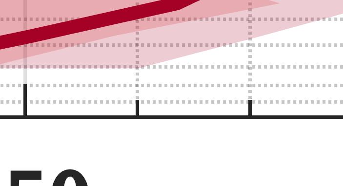
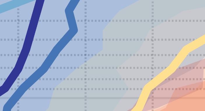
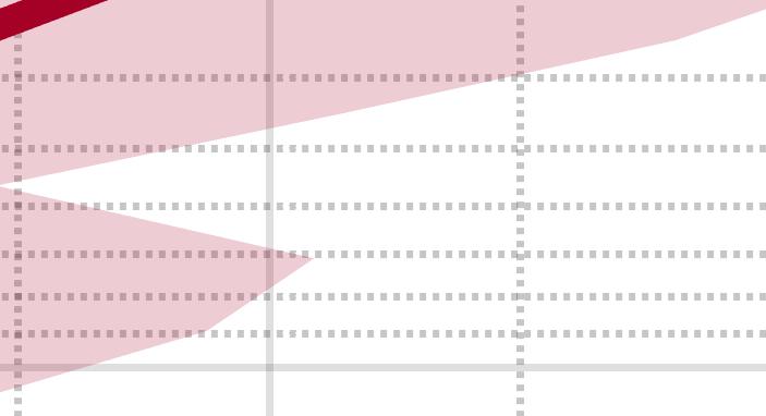
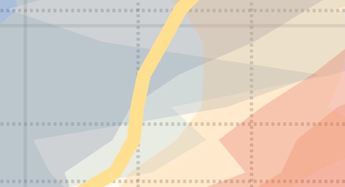
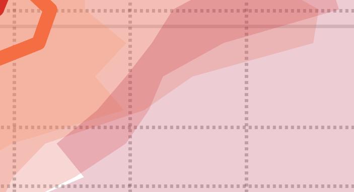
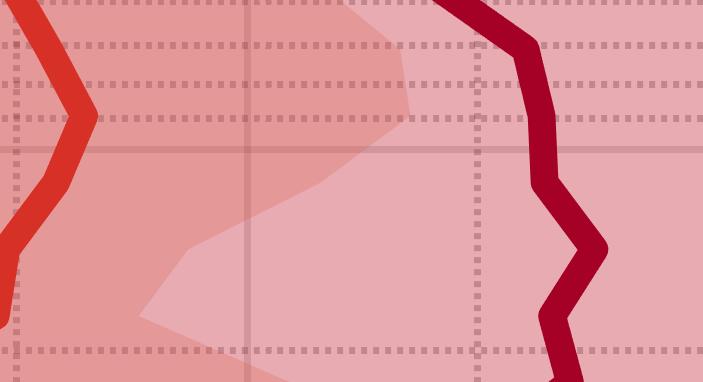
81 Figure 14. Mean temperatures for the 8 DDs. The shaded regions represent 1-σ variabilities.

82 CO 2 Density (cm -3 ) Temperature (K) Figure Local Time (h) Temperature (in color) binned as a function of CO 2 density (vertical axis) and local 50 time (horizontal axis). White bins signify no data. Measurements are constrained to latitudes between 60 N and 60 S.

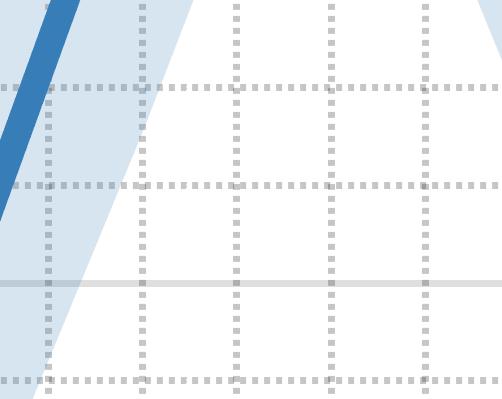
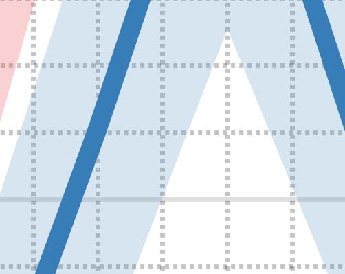
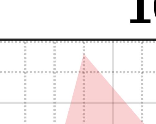
83 Figure 16. Temperature as a function of Martian local time at two constant CO 2 density levels: 10 6 cm 3 (red) and 10 9 cm 3 (blue). Measurements are constrained to latitudes between 60 N and 60 S. The shaded regions represent 1-σ variabilities.

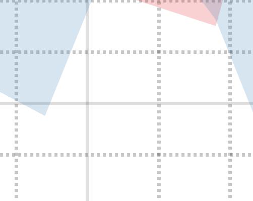
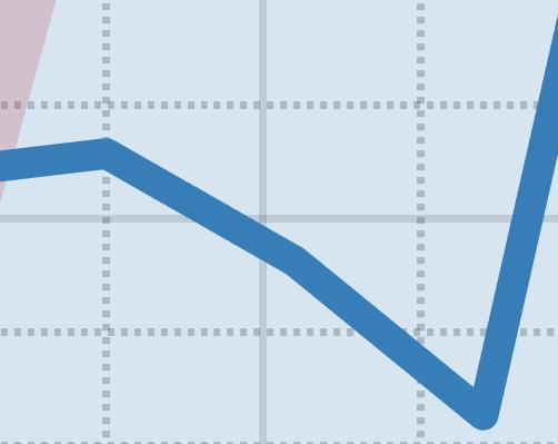
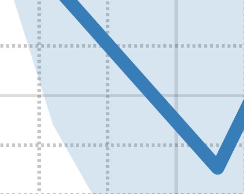
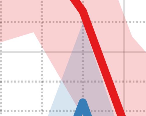
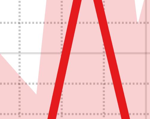
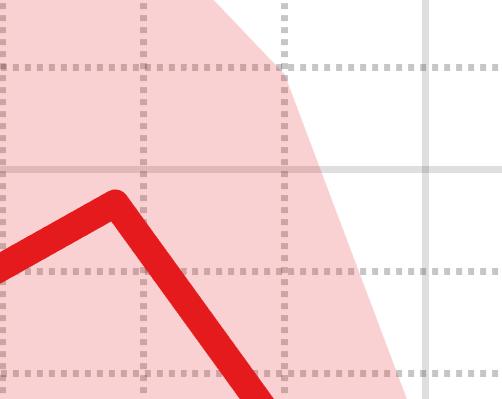
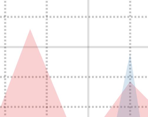
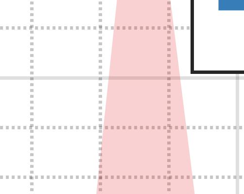
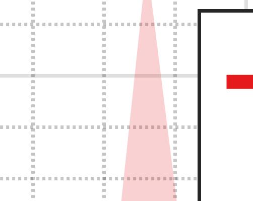
84 Figure 17. Ar temperature as a function of latitude at two constant CO 2 density levels: 10 6 cm 3 (red) and 10 9 cm 3 (blue). Measurements are constrained to local times between 9 AM and 5 PM. The shaded regions represent 1-σ variabilities.

85 CO 2 Density (cm -3 ) DD6 DD3 DD5 DD7 DD8 DD4 DD1 DD [O] / [CO 2 ] Figure 18. The [O]/[CO 2 ] ratios for each of the 8 DDs.

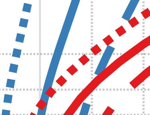
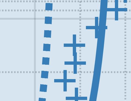
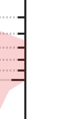
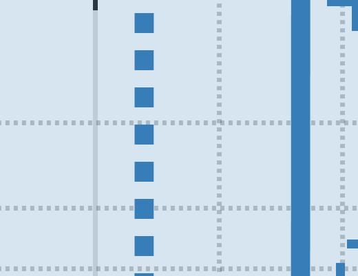
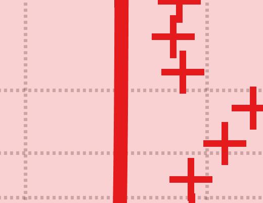
86 Figure 19. Comparison of modeled temperature profiles with NGIMS data. The model temperature profiles for equatorial latitudes at 12 PM (red lines) and 12 AM (blue lines) compared to DD2 (red +) and DD6 (blue +) NGIMS temperature profiles. The solid lines are for models calculated with the nominal O-CO 2 collisional de-excitation rate of k = cm 3 s 1, the dotted lines for k = cm 3 s 1, and the dashed lines for k = cm 3 s 1. The shaded regions represent 1-σ variabilities of the NGIMS temperatures.

87 CO 2 Density (cm -3 ) Temperature (K) Local Time (h) 50 Figure 20. The temperature at equatorial latitudes versus local time in the 1D model.

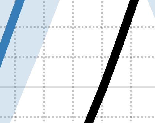
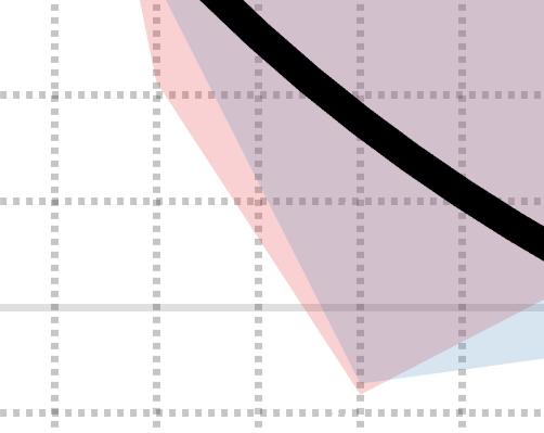
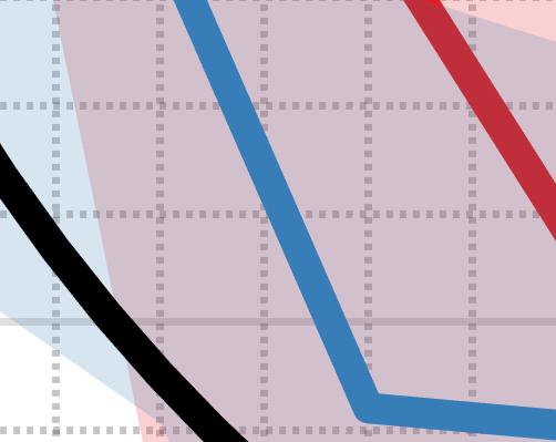
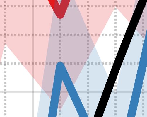
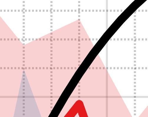
88 Figure 21. Comparison of the observed diurnal variation of the temperature at CO 2 densities of 10 6 cm 3 (red) and 10 9 cm 3 (blue) with the diurnal variation of the temperature in the 1D model at a CO 2 density of 10 7 cm 3 (black). The shaded regions represent 1-σ variabilities.