On the Origins of Mars' Exospheric Non-Thermal Oxygen. Component as observed by MAVEN and modeled by HELIOSARES

Transcription

1 On the Origins of Mars' Exospheric Non-Thermal Oxygen Component as observed by MAVEN and modeled by HELIOSARES Leblanc F. 1, Chaufray J.Y. 1, Modolo R. 2, Leclercq L. 1,6, Curry S. 3, Luhmann J. 3, Lillis R. 3, Hara T. 3, McFadden J. 3, Halekas J. 4, Schneider N. 5, Deighan J. 5, Mahaffy P. R. 7, Benna M. 7, R.E. Johnson 6, Gonzalez-Galindo F. 8, Forget F. 9, M.A. Lopez-Valverde 8, F. G. Eparvier 5 and B. Jakosky 5 1 LATMOS/IPSL, UPMC Univ. Paris 06 Sorbonne Universités, UVSQ, CNRS, Paris, France 2 LATMOS/IPSL, UVSQ Université Paris-Saclay, UPMC Univ. Paris 06, CNRS, Guyancourt, France 3 Space Science Laboratory, University of California, Berkeley, CA, USA 4 University of Iowa, Department of Physics and Astronomy, IA, USA 5 Laboratory for Atmospheric and Space Physics, University of Colorado, Boulder, CO, USA 6 Department of Material Science, University of Virginia, Charlottesville, USA 7 NASA Goddard Space Flight Center, Greenbelt, MD, USA 8 Instituto de Astrofısica de Andalucıa, CSIC, Granada, Spain. 9 Laboratoire de Météorologie Dynamique (LMD/IPSL), Sorbonne Universités, UPMC Univ Paris 06, PSL Research University, Ecole Normale Supérieure, Université Paris-Saclay, Ecole Polytechnique, CNRS, Paris, France This article has been accepted for publication and undergone full peer review but has not been through the copyediting, typesetting, pagination and proofreading process which may lead to differences between this version and the Version of Record. Please cite this article as doi: /2017JE005336

2 Abstract: The first measurements of the emission brightness of the oxygen atomic exosphere by Mars Atmosphere and Volatile EvolutioN (MAVEN) mission have clearly shown that it is composed of a thermal component produced by the extension of the upper atmosphere and of a non-thermal component. Modeling these measurements allows us to constrain the origins of the exospheric O and, as a consequence, to estimate Mars' present oxygen escape rate. We here propose an analysis of three periods of MAVEN observations based on a set of three coupled models: a hybrid magnetospheric model (LatHyS), an Exospheric General Model (EGM) and the Global Martian Circulation model of the Laboratoire de Météorologie Dynamique (LMD-GCM), which provide a description of Mars' environment from the surface up to the solar wind. The simulated magnetosphere by LatHyS is in good agreement with MAVEN Plasma and Field Package instruments data. The LMD-GCM modeled upper atmospheric profiles for the main neutral and ion species are compared to NGIMS/MAVEN data showing that the LMD-GCM can provide a satisfactory global view of Mars' upper atmosphere. Finally, we were able to reconstruct the expected emission brightness intensity from the oxygen exosphere using EGM. The good agreement with the averaged measured profiles by IUVS during these three periods suggests that Mars' exospheric non-thermal component can be fully explained by the reactions of dissociative recombination of the O 2 + ion in Mars' ionosphere, limiting significantly our ability to extract information from MAVEN observations of the O exosphere on other non-thermal processes, such as sputtering.

3 I Introduction Before the insertion of MAVEN around Mars in September 2014, no Martian mission was specifically dedicated to the observation of Mars' upper atmosphere and exosphere (Jakosky et al. 2015). MAVEN was conceived around a set of instruments dedicated to the characterization of these regions of Mars with the goal to constrain the mechanisms leading to Mars' atmospheric escape to space (Lillis et al. 2015). Atmospheric escape is primarily driven by the solar wind and by the solar UV/EUV flux. The key goal of MAVEN is, therefore, to constrain how Mars' atmospheric erosion might have changed over time with respect to these two solar forcing. The observation of Mars' atmospheric escape is far from being trivial. It is not possible with a single spacecraft to obtain an instantaneous global 3D view of the different channels of atmospheric escape. Even in the case of the planetary ion escape, that can be directly measured by ion mass and energy spectrometers like SWIA/MAVEN (Halekas et al. 2013) and STATIC/MAVEN (McFadden et al. 2015), reconstructing the global flux requires accumulating several months of MAVEN's observations (Brain et al. 2015) or of ASPERA-3/Mars Express data (Nilsson et al. 2010). A direct measurement of the neutral escape flux is instrumentally not achievable today, so that indirect measurements are required to constrain this component. This is particularly true for heavy atmospheric species like oxygen, carbon and nitrogen atoms which are difficult to observe far from Mars due to their very low density, contrary to light species like hydrogen atoms (Chaffin et al. 2014). Fortunately, an indirect signature of Mars' neutral oxygen escape was observed for the first time by ALICE/ROSETTA (Feldman et al. 2011) and confirmed by the Imaging Ultraviolet Spectrograph (IUVS)/MAVEN (Deighan et al. 2015). These authors confirmed the existence of two energy components in the Martian atomic oxygen exosphere predicted by McElroy et al. (1972) and since then, modeled by few groups (for the most recent published models see Valeille et al. 2010a and b; Yagi et al. 2012; Lee et al. 2015a and b, Gröller et al. 2014). This dual composition of the exosphere is obvious when looking at the variation in altitude of the brightness of the nm atomic oxygen resonant emission. This variation displays a clear two slopes evolution with increasing altitudes, with a fast

4 decrease of the emission brightness just above the exobase followed by a much slower decrease from typically 600 km above the surface of Mars (Deighan et al. 2015). The less energetic component associated with the low altitude fast decrease of the emission brightness and a small scale height is attributed to the thermal expansion of Mars' atomic oxygen component above the Martian exobase and is usually described as the thermal component of the exosphere (Chaufray et al. 2015). The more energetic component above 600 km is thought to be produced essentially by two processes occurring in Mars' upper atmosphere, the dissociative recombination of the most abundant ion, O + 2, in Mars' ionosphere (Lee et al. 2015b) and the sputtering of the upper atmosphere by precipitating pick-up ions (Luhmann and Kozyra 1992; Leblanc et al. 2015). These processes are thought to be the two main channels of Mars' neutral atmospheric oxygen escape (Chaufray et al. 2007). Therefore, since direct measurement of the neutral escape is not possible, modeling the different components of the atomic oxygen exosphere remains the most direct approach to constrain Mars' oxygen neutral escape (Lillis et al. 2015). The University of Michigan has developed a set of numerical tools describing the state of Mars' atmosphere from its surface to its exobase, the Mars Global Ionosphere-Thermosphere Model (M- GITM; Bougher et al. 2015a) as well as the Mars Adaptive Mesh Particle Simulator (M-AMPS) a model describing the energetic component of Mars' associated exosphere as formed from the dissociative recombination of the main Martian ionospheric ion O + 2 (Valeille et al. 2010a and b; Lee et al. 2015a). Both M-GITM and M-AMPS have been coupled in order to describe the detailed spatial distribution of the atomic oxygen exosphere for any Mars' season and solar conditions. The outputs from these models were compared to the first set of MAVEN observations of the upper atmosphere of Mars for M-GITM (Bougher et al. 2015b) and of the oxygen exosphere for M-AMPS (Lee et al. 2015b). In a similar effort, in the frame of a project named HELIOSARES, the LMD-GCM (Forget et al. 1999) was first extended to include the ionosphere up to the photo-chemical boundary (Gonzalez- Galindo et al. 2013) and later up to the exobase by decoupling the ion and neutral transports in Mars' upper atmosphere (Chaufray et al. 2014). This model was then coupled to an exospheric

5 model of Mars, in order to derive the spatial structure of Mars' energetic exospheric components as produced from both dissociative recombination of the O + 2 ion in Mars' ionosphere and by sputtering of the upper atmosphere by incident pick-up ions precipitating from Mars' magnetosphere into its atmosphere. In order to reconstruct the ion precipitation, the LMD-GCM and EGM models have been coupled to a magnetospheric hybrid model, LatHyS, which describes the interaction of the solar wind with Mars (Modolo et al. 2016). This set of models provides a 3D description of Mars' environment from its surface to the solar wind for any Martian seasons and solar activities. The goal of this paper is to present the first set of comparisons between HELIOSARES models and MAVEN observations. We will here specifically focus on the different signatures in MAVEN data from Mars' upper atmosphere up to Mars' magnetosphere relevant to the reconstruction of the neutral atmospheric oxygen exosphere. As stated above, the IUVS observations of Mars' oxygen exosphere are the most useful measurements for constraining any model aiming to estimate Mars' atmospheric neutral oxygen escape. This is why this paper is organized around three set of exospheric measurements performed during the first two years of MAVEN scientific operations. For each of these three periods, we will present, in section II, the typical profile of the observed exospheric emission brightness as measured by IUVS, NGIMS measurements of Mars' upper atmosphere and STATIC and SWIA reconstructed precipitating flux. In section III, we will present HELIOSARES set of models and in section IV an example of results obtained from these set of coupled models. In section V, MAVEN and HELIOSARES will be compared for the three periods, which will be followed by a discussion of this comparison in section VI and a conclusion in section VII. II MAVEN data II.1 Exospheric density profiles: Imaging UltraViolet Spectrograph (IUVS) IUVS (McClintock et al. 2014) on board MAVEN is a remote sensing instrument whose FUV channel is intensified to maximize the signal from the faint exospheric emission from the oxygen triplet line at nm. IUVS has two different modes, a normal mode with a moderate spectral resolution of 200

6 and an echelle mode with much higher spectral resolution of ( / with the wavelength). For the reconstruction of the nm oxygen emission brightness above the exobase, we used the normal mode and the outbound part of the orbit during which the O emission is also observed from the disk up to the apoapsis (Chaufray et al. 2015; Deighan et al. 2015). Considering the period from November 2014 to August 2016, we selected three periods of observations during which IUVS covers the dayside exosphere providing a good signal/noise ratio of the oxygen emission brightness from the exobase up to several thousand km in altitude. Each period covers around 20 days of consecutive observations corresponding to 11 to 26 observations of the exospheric atomic oxygen emission line covering a relatively narrow range of solar zenith angle (SZA), MSO (Mars Sun Orbital) longitude and latitude because of the slow precession of MAVEN periapsis. We excluded orbits during which the emission of the oxygen atom could not be clearly identified in IUVS spectra. In Table 1, we listed the selected orbits for each of these three periods.

7 Period Number of orbits Orbit Numbers Ls ( ) D (AU) SZA ( ) Longitude (MSO) Latitude (MSO) EUV (10-4 W/m²) 0.1-7nm nm nm 07/16/ /04/ , 3504, 3508, 3512, 3518, 3522, 3526, 3530, 3536, 3540, 3544, 3558, 3564, 3570, 3576, 3600 [187, ] 1.44 [15.9, 21.7 ] [9.4, 11.5 ] [4.6, 18.2 ] 2.5± ± ± , 403, 405, 407, 410, 412, 414, 416, 12/13/ /01/ , 426, 438, 440, 444, 448, 452, 456, 460, 468, 474, 478, 482, 486, 492, 496, [251.75, ] 1.38 [51.0, 61.3 ] [-52.4, ] [19.3, 36.8 ] 4.48± ± ± /09/ /01/ , 708, 756, 762, 786, 790, 794, 798, 804, 808, 812 [288.8, ] 1.42 [76, 85 ] [-25, -23 ] [-50, - 14 ] 4.2± ± ±0.001 Table 1: IUVS selected set of observations for the three periods (L1b v04_r01 product). The Solar zenith angle (SZA), MSO longitude and latitude correspond to the range covered by all the scans selected to reconstruct the average emission brightness profile. Ls is Mars' solar longitude. D is for Mars' heliocentric distance. The EUV flux is measured by EUV/LPW instrument on MAVEN. We used L2_v07_r02 products (Eparvier et al. 2015).

8 The difficulty to extract accurately the emission brightness of the O triplet from the FUV spectra is, first, related to the decrease of the signal/noise ratio with increasing altitude. Secondly, the nm emission is spectrally close to the very bright Lyman emission line whose wings can contribute significantly to the measured spectra around nm in particular at high altitudes when the brightness contrast between these two lines get more and more important (Chaufray et al. 2015). Therefore, in order to reduce the uncertainty when deriving the oxygen emission brightness at high altitude, we first reconstructed the average spectra between two altitudes using all individual spectra measured during the listed orbits in Table 1. Typically, between 115 and 400 km in altitude, we used a 15 km altitude resolution, between 400 and 700 km a 30 km resolution, between 700 and 1200 km a 50 km resolution and above a 200 km resolution. Each spectrum is then built from 40 to 700 individual spectra, a number which is tuned to optimize the retrieved signal/noise ratio. From this average spectra, we then developed a dedicated approach to integrate the emission line associated with the oxygen triplet emission lines by fitting the spectra, around these emission lines, with a combination of exponential and linear laws in order to estimate the background and the contribution from the wing of the Lyman emission line. The uncertainty of the integrated emission brightness is estimated after subtraction of the background from the residual on each average spectra, around the oxygen emission lines. FIGURE 1 In Figure 1, we plotted the profiles of the nm triplet oxygen emission brightness measured by IUVS during the three periods described in Table 1. As shown in this figure, the three profiles are significantly different, essentially because they cover different range of SZA and have been measured at different distance to the Sun (see Table 1 and Figure 2). As an example, the brightness intensity at 300 km in altitude which is essentially due to the thermal component of the exosphere, changes from 324±10 Rayleigh (R) at SZA 19 (panel a), to 484±10 R at SZA 56 (panel b) down to

9 126±6 R at SZA 80 (panel c). The 33% smaller intensity of the thermal emission brightness at SZA 19 with respect to the measured brightness at SZA 56 can be explained essentially by the 26% smaller EUV flux at Mars between these two periods (column 11, Table 1), as measured by EUV/LPW instrument on MAVEN (Eparvier et al. 2015). Moreover, these two profiles were obtained for different Martian seasons, beginning of autumn for panel a (Ls=[187, ]) and end of autumn for panel b (Ls=[251.75, ]). Eventually, the geometry of the observations (the Field of View, FOV, of IUVS) needs to be considered for this comparison as shown in section V.3. A remarkable feature on these three panels is the clear change of slope of the emission brightness with increasing altitude around 600 km. This is clearly the signature of a change of the energy distribution of the exospheric oxygen population, with a small scale height below, associated to the thermal component, and a much higher scale height above. The scale heights of the thermal and non-thermal components of the exosphere are found to increase with SZA: -from 95 km at SZA 19 (panel a), to 119 km at SZA 56 (panel b) up to 142 km at SZA 80 (panel c), below 600 km - from 1087 km at SZA 19 (panel a), to 1610 km at SZA 56 (panel b) up to 2340 km at SZA 80 (panel c), above 600 km. Below 600 km, the increasing scale height with SZA is probably due to the increasing proportion of non-thermal oxygen particle within this altitude range, whereas above 600 km the increase scale height with SZA will be shown in section V.3 to be due in part to the FOV of IUVS during these observations. At 1000 km in altitude, the measured brightness intensity is larger at SZA 56 (panel b), 19.6±4 R, than at SZA 19 (panel a), 11±3 R, a difference within the uncertainty when the 25% difference in solar flux intensity is taken into account. II.2 Thermospheric and Ionospheric density profiles: Neutral Gas and Ion Mass Spectrometer (NGIMS) For the three periods displayed in Table 1, we also reconstructed the average measured densities along MAVEN path through the upper atmosphere of Mars as measured by NGIMS/MAVEN (Mahaffy

10 et al. 2015a). Because IUVS observations of the Martian exosphere are performed from the periapsis path up to the apoapsis, IUVS observations cover the opposite side of Mars with respect to the periapsis position (Figure 2). As a consequence, NGIMS in situ measurements of the thermosphere/ionosphere cannot be directly associated to IUVS exospheric measurements but are presented here essentially to support our comparison between HELIOSARES simulations and MAVEN observations. In Table 2, we summarize the main characteristics of NGIMS coverage (also in Figure 2). The average density profiles measured by NGIMS during the three periods in Fig. 1 are reconstructed in order to reduce the dependency of the density profile with respect to short term variability (in particular gravity waves, England et al., 2017). We also focused on the major heavy species of Mars' atmosphere: CO 2, N 2, O, O + 2 and CO + 2 and restricted our analysis to the inbound part of the orbit to limit the SZA coverage of each period and to avoid any calibration issue during the outbound part of the orbit, as an example, due to interaction of the gas with the surface of the instrument (Mahaffy et al. 2015b). FIGURE 2 Period Number of inbound paths for each species Ls ( ) Longitude (MSO) Latitude (MSO) SZA 07/16/ /04/ (O), 95 (N 2 ), 95 (CO 2 ), 43 (O + 2 ), 43 (CO + 2 ) [187, ] [135, -153 ] [-44, -4 ] [121, 171 ] 12/13/ /01/ (O), 79 (N 2 ), 79 (CO 2 ), 44 (O + 2 ), 44 (CO + 2 ) [251.75, ] [153, -134 ] [10, 56 ] [113, 162 ] 02/09/ (O), 78 (N 2 ), [288.8, [54, 122 ] [-11, 30 ] [54, 117 ]

11 03/01/ (CO 2 ), ] (O + 2 ), 44 (CO + 2 ) Table 2: NGIMS measurements during the three periods considered in Table 1. L2 v06_r02 level was used for this analysis (open and close source modes as well as ion mode). The number of inbound paths correspond to the number of individual density profiles that were averaged to reconstruct the profiles displayed in Figure 3. The profiles displayed in Figure 3c were measured near the terminator, so that NGIMS measurements are composed of nightside measurements at low altitude (below 150 km) and of dayside measurements at high altitude. Panel a density profiles were obtained at the largest SZA within these three periods. The slope of the neutral profiles displayed in Figure 3 are clearly organized with respect to the mass of each species. As an example, in panel a, the scale height of the CO 2 species (when measured between 160 and 220 km in altitude) is equal to 7.4 km whereas the N 2 species scale height is equal to km, a ratio of the scale height equivalent to the ratio of the respective mass. In another way, between 160 and 220 km, there is a clear mass fractionation with altitude which, as a first order, corresponds to the same neutral temperature. The profile displayed in Figure 3c is the only profile measured on the dayside, displaying a clearly larger scale height above 150 km (11.5 km for CO 2 ) than for the two other periods. Panel b profiles suggest that the atmosphere at that time and location was slightly colder than the atmosphere corresponding to panel a profiles. This might be due to the difference in season, sampled by NGIMS, panel a profile being measured during the early autumn season whereas panel b was measured during late autumn season. The O species is observed to become the main atmospheric species with increasing altitude and decreasing SZA (from panels a to c). The dispersion of the neutral density profile (from one to another measured profile as indicated by the horizontal bars) is largest at low altitude, showing that below 180 km the neutral density profile is significantly impacted by the short time variability of the atmosphere and less above.

12 FIGURE 3 Contrary to the neutral atmosphere, the slopes of the ion species are not mass dependent and + appear similar between 140 and 200 km in altitude. The LMD-GCM simulated profiles of the CO 2 species usually decrease faster with increasing altitude than O + 2 (Chaufray et al. 2014), a difference that we will discuss in section V.5. As illustrated in panel c, Mars' ionospheric densities are highly dependent on the solar flux; a clear increase of the ion density was observed along MAVEN path through the terminator when moving from 150 km to 155 km in altitude. II.3 Precipitating flux at the exobase: SupraThermal and Thermal Ion Composition (STATIC) and Solar Wind Ion Analyzer (SWIA) Precipitating heavy pick-up ions into Mars' atmosphere have been predicted for a long time (Luhmann et al. 1992; Chaufray et al. 2007; Lillis et al. 2015) but were observed only sporadically during solar energetic event by ASPERA-3/Mars Express (Hara et al. 2011). However, thanks to MAVEN s higher temporal, angular and energy coverages, the ion mass spectrometers STATIC and SWIA on board MAVEN were able to provide the first direct measurements of precipitating pick-up ion flux during nominal solar conditions (Leblanc et al. 2015). Hara et al. (2016) published a first detailed analysis of the dependency of this precipitation with respect to various solar drivers, concluding that the precipitating flux is globally organized, as expected, with respect to the orientation of the solar wind convection electric field. In the following, we will present the typical precipitating flux measured during the three periods selected in section II.1. As in Leblanc et al. (2015) and Hara et al. (2016), we selected all orbit segments between 200 and 350 km in altitude and reconstructed the precipitating flux by focusing on SWIA cs product (4 s temporal resolution), STATIC ca (4 s resolution) and STATIC d0 (between 32 s and 128 s resolution) products. We then selected the anodes of these two instruments whose FOV was at less than 75 from the zenith

13 direction. When the angular coverage of a given instrument covered more than 65% of the cone angle of 75 width centered along the zenith direction, we selected the measurement to reconstruct the average precipitating flux. Contrary to NGIMS measurements, we selected the inbound and outbound segments. The associated latitudinal/longitudinal coverage is therefore more extended than for NGIMS coverage (Table 3 and Figure 2). SWIA cs product has an angular coverage of with a resolution of and an energy resolution of 14.5% (with 48 logarithmically spaced energy steps). STATIC has an angular coverage of , with the ca product providing an angular resolution of and 16 bins in energy but without mass resolution whereas the d0 product provides the same angular resolution with 32 bins in energy and 8 bins in mass. For the d0 product, we focused on the mass range between 15 and 17 amu. Table 3 provides the MSO longitude/latitude coverage and the number of measurements used for each of the three periods.

14 Period Instrument product Time resolution (s) Longitude (MSO) Latitude (MSO) Number of used km orbit portions /Total number of available orbits. Percentage of the FOV covered by the instrument Mean Solar Wind density (cm -3 ) Mean Solar Wind velocity V SW (MSO) (km/s) Mean IMF B SW (MSO) (nt) Mean intens ity of the IMF (nt) Mean Solar wind electric field of convection E SW = -V SW B SW (µv/m) 07/16/ /04/2016 SWIA cs 4 STATIC ca 4 STATIC d0 32 [15-17 amu] [140, ] [150, ] [140, ] [-40, 20 ] [-40, 20 ] [-40, 20 ] 208/ / / [-460, 25.4, 3.35] [- 0.03±0.07, 0.04±0.08, 0.05±0.05] 2.8 [24, -212, -50] 12/13/ /01/2015 SWIA cs 4 [160, -60 ] [30, 70 ] 178/ STATIC ca 4 [180, -80 ] [30, 60 ] 7/ STATIC d0 [160, [30, 60 ] 3/ [15-17 amu] 110 ] 4.84 [-382, 30, - 3.9] [0.2±0.05, -0.1±0.07, -0.02±0.04] 4.5 [-14.3, -14.1, -314]

15 02/09/ /01/2015 SWIA cs 4 [50, 160 ] STATIC ca 4 [50, 160 ] STATIC d0 128 [60, 100 ] [15-17 amu] [-10, 45 ] [-10, 45 ] [-10, 10 ] 217/ / / [-329; 24.1, 0.07] [0.23±0.05, -0.14±0.07, 0.07±0.04] 3.9 [-22.5, -132, -154] Table 3: SWIA and STATIC measurements used to reconstruct the precipitating pick-up ion flux. The number of km orbit segments is for the number of sequences of observation during which the average FOV covered by a given instrument was more than 65% for SWIA cs and STATIC ca (60% for STATIC d0) of the 75 cone angle along the zenith direction. The percentage of the FOV coverage is the average percentage of this cone angle covered by each instrument. The mean solar wind characteristics are the mean measurements by SWIA and MAG instruments when MAVEN was in the solar wind during that periods. The mean solar wind electric field of convection is the mean value of all electric fields of convection.

16 As shown in Figure 4, there is, in general, good agreement between the reconstructed precipitating flux derived from SWIA cs (red lines in Figure 4) and the one derived from STATIC ca (blue lines in Figure 4), despite the much lower sampling rate of STATIC with respect to SWIA. STATIC is indeed usually pointing along the ram direction whereas SWIA is pointing towards the incident solar wind direction, a much better orientation to cover the zenith angle direction. Because STATIC d0 product was measured with a 8 to 16 times longer temporal resolution than SWIA cs and STATIC ca, much less individual measurements were available during the 200 to 350 km portion of the orbit (see the 6th column of Table 3). As a consequence, the reconstructed precipitating flux using d0 measurement for the mass range 15 to 17 amu (focusing on the O + ion, the most abundant expected precipitating heavy ion, Lillis et al. 2015) is usually much less well resolved. Because SWIA cs and STATIC ca fluxes were reconstructed for all ions, it is however interesting to use the d0 measured precipitating flux to estimate the proportion of SWIA cs and STATIC ca measured fluxes associated to O + precipitating ion. The d0 reconstructed flux appears to be in good agreement (within the uncertainty) with the measured SWIA flux above 1000 ev, suggesting that O + is indeed the main precipitating ion above this energy. FIGURE 4 The ion composition of the precipitating flux might depend, to first order, on the local time. During 02/09/ /01/2015 period (panel c), MAVEN sampled day and night sides equatorial region near the dusk terminator, whereas during 12/13/ /01/2015 period, MAVEN periapsis was at high latitude on the nightside. At the end, during 07/16/ /04/2016 period, MAVEN periapsis was also covering equatorial nightside regions but at lower SZA than for the 12/13/ /01/2015 period. Therefore, we expect that during 02/09/ /01/2015, the precipitating flux should have been in part composed of penetrating solar wind particles below 1000 ev, as suggested by the large difference between the d0 measurement of the amu mass range (green line in panel c) and

17 SWIA cs measurement (red line) for all masses. On the contrary, at high latitude, in the nightside, precipitating solar wind particles should be much less abundant than the precipitating planetary ions as suggested in panel b, where the amu measured flux is essentially similar to the all masses measured flux by SWIA at all energy. The third period, 07/16/ /04/2016, panel a, corresponds to a case between these two other periods, in which the low mass particles seem to contribute significantly to the measured flux, at least below 500 ev. Unfortunately, above 500 ev, measurements of the mass range amu following our criteria were not available. In terms of intensity, as shown by Hara et al. (2016), we might expect, to first order, that the precipitating flux intensity is organized in Mars Solar Electric (MSE) frame where X points from Mars towards -V SW the solar wind velocity, +Z is parallel to E SW =-V SW xb SW with B SW as the interplanetary magnetic field vector (Table 3) and Y completes the orthogonal coordinate set. Hara et al. (2016) suggested that the intensity of the flux of precipitating ions peaked on the hemisphere towards which the E SW field pointed (the -E SW hemisphere). In Table 3, we calculated the mean electric field of convection, showing that: during period 12/13/ /01/2015, the electric field was oriented towards the -Z MSO direction, MAVEN was therefore sampling the -E SW nightside hemisphere, during 02/09/ /01/2015, the electric field was within the Y MSO -Z MSO plane at 45 from the -Z MSO and -Y MSO axis, MAVEN was therefore sampling the -E SW dayside/nightside hemisphere, during 07/16/ /04/2016, the electric field of convection was oriented along the -Y MSO direction, MAVEN was therefore sampling +E SW nightside hemisphere. Comparing the intensity of the measured SWIA flux during these three periods, the measured flux at low energy (100 ev) is significantly larger during the 12/13/ /01/2015 period with respect to the two other periods. As shown in Table 3, during the 12/13/ /01/2015 period, the electric field of convection was the largest which could even enhance this difference. Moreover, the measured flux is larger at 1000 ev during the 07/16/ /04/2016, that is for the only period

18 which sampled the +E sw hemisphere. Such an energy dichotomy of the organization of the precipitating flux was suggested by modeling (Lillis et al. 2015) but not confirmed by MAVEN observations based on a much larger statistic than in this present work (Hara et al. 2016). III HELIOSARES set of models In order to describe properly how the mass and energy of the solar wind are deposited into Mars' atmosphere, it is now well understood that Mars needs to be considered as an integrated system (Bougher et al. 2002) in which energy and mass from the Sun impact all layers of Mars, from its surface to its magnetosphere (Leblanc et al. 2009). These findings motivated the HELIOSARES project whose main goal was to couple three independent models of Mars' environment: Mars LMD-General Circulation Model (LMD-GCM), Mars LATmos HYbrid Simulation (LatHyS) magnetospheric model and Mars Exospheric Global Model (EGM). HELIOSARES LMD-GCM is an extension of the 3D LMD-GCM (Forget et al. 1999) which integrates the description of the thermosphere (Angelats-i-Coll et al. 2005, Gonzalez-Galindo et al. 2009) and of the ionosphere (Gonzalez-Galindo et al. 2013), including a dynamic module for the ion (Chaufray et al. 2014) in order to be able to describe the ion density above the photochemical boundary and to improve the coupling with the exosphere and magnetosphere. Details on this model can be found in Chaufray et al. (2014) and references therein. LatHyS is a 3D parallelized model of Mars' magnetosphere as formed by the interaction of Mars' atmosphere with the solar wind. Based on a hybrid formalism, LatHyS is well suited to describe the pick-up ions precipitating into Mars' atmosphere, in particular, kinetic effects which are very important in the magnetosphere. Details on this model can be found in Modolo et al. (2016). The Exospheric Global Model was developed to solve the Boltzmann equation in order to provide a description of Mars' exosphere, when produced from Mars' ionospheric chemistry and Mars' thermospheric sputtering by the heavy pick-up ions precipitating towards Mars' atmosphere. It is a 3D multispecies collisional parallelized model that can follow the fate of non-thermal particles (that

19 is whose energy is significantly larger than the local thermal energy). This model was described in Leblanc et al. (2017), in particular the treatment of collisions using universal cross sections of Lewkov and Kharchenko (2014). The EGM is a 3D Monte Carlo which uses the LMD-GCM inputs to describe the background neutral atmosphere, typically from 120 km up to 250 km above the surface and to model the photo-chemical sources of non-thermal particles in Mars' upper atmosphere. As an example, the dissociative recombination of the main O + 2 ion into two non-thermal O atoms is taken into account being thought to be the main reactions producing Mars' energetic exospheric component (Chaufray et al. 2007; Valeille et al. 2010a and b). Non-thermal O test particles are followed through Mars' upper atmosphere taking into account their collision with the background atmosphere up to 600 km in altitude. Above this altitude, we suppose that collisions are negligible. In order to describe the effect of precipitating ions on Mars' atmosphere, we use LatHyS simulations to reconstruct the O + precipitating flux at 300 km in altitude (consistently with the method used to reconstruct this precipitating flux from MAVEN measurement). This 3D flux map (energy, latitude, longitude) is used as input in EGM. Any atmospheric particle which gained energy by collision with a non-thermal particle is also followed. Because it is numerically not feasible to follow all test particles, we had to set a lower energy threshold below which a test particle is supposed to be thermalized and is no longer followed; this very low energy population is therefore neglected in the reconstruction of the non-thermal component in the exosphere. It should be noted that the heating of the thermosphere that could be induced by this low energy population is partially taken into account in the LMD-GCM by introducing a UV heating efficiency (Gonzalez-Galindo et al. 2005). Typically, we used a threshold defined as a percentage of the local escape energy, usually equal to 5%. As explained in Leblanc et al. (2001), such a limit on the non-thermal component of the exosphere implies that the energetic exospheric density will be underestimated below typically 400 km in altitude. Because, as suggested by Figure 1, this altitude is significantly lower than the altitude at which the thermal exospheric component density starts to be smaller than the non-thermal exospheric component, our description of the exosphere should not be significantly impacted by this

20 limit. EGM provides a description of the main heavy neutral component of Mars' exosphere (oxygen and carbon related species, as well as N 2 species). The thermal component of the exosphere is reconstructed using a 3D kinetic approach to solve the Liouville equation using Mars' exobase characteristics (Yagi et al. 2012) for the main species at the exobase (that is, O, H, CO 2, CO, H 2 and N 2 ). FIGURE 5 The main goals of HELIOSARES was to couple these three models in order to describe Mars' environment from its surface to the exosphere for any given season, solar wind conditions and solar activity. Figure 5 provides an illustration how these three models are presently coupled (left panel) and how Mars' environment from the surface up to the solar wind is reconstructed (right panel). The LMD-GCM simulation outputs (a 3D description of the density, velocity and temperature of the main neutral and ion species in Mars' thermosphere/ionosphere at a given season and solar activity, considering the most probable scenario of dust activity) are used to define the background atmosphere and ionosphere of EGM, as well as to define Mars' atmosphere in LatHyS model (the lower boundary of this model required to compute the ionospheric dynamics). The reconstructed exospheric composition and density by EGM is used to describe Mars' exosphere in LatHyS model. LatHyS is then used to model Mars' magnetosphere as well as the longitude-latitude precipitating flux at 300 km in altitude, which is used in EGM to calculate the sputtered energetic exospheric component associated to this precipitation. In the end, to compare the outputs of HELIOSARES with IUVS measurement, we used a 3D radiative transfer model which used the reconstructed 3D multispecies exosphere calculated by EGM (including the thermal component). This model was presented in Chaufray et al. (2016). IV HELIOSARES modeled Mars' environment

21 In this section, we present one example of a coupled simulation by describing the modeled magnetosphere (section IV.1), the modeled thermosphere/ionosphere (section IV.2) and associated exosphere (section IV.3). We chose to focus on one Mars' season at Ls=180, modeled for mean solar activity (we use the definition for medium conditions as given in Gonzales-Galindo et al. (2005)) and nominal solar wind conditions (see Table 4). IV.1 Mars' induced magnetosphere as described by LatHyS For this simulation, we considered the solar wind parameters corresponding to the 07/25/2016 MAVEN orbit between 8:00 and 13:00 UTC (Table 4). During that orbit, MAVEN closest approach occurred at 10h23. The subsolar point was at an eastern longitude of 284 and a latitude of -5 so that the major structure of the crustal magnetic field (at 180 eastern longitude in the southern hemisphere; Acuna et al. 2001) was around 6 hour in local time. Ls ( ) Solar activity Solar wind density (cm -3 ) Solar wind velocity (km/s) IMF (nt) Proton temperature (ev) MAVEN measurements Mean 3.9 ± 0.4 Vx = -408 ± 5.3 Vy = 33.8 ± 4.5 Vz = 4.3 ± 6.4 Bx = -1.0 ± 0.7 By = 0.79 ± 0.32 Bz = 0.32 ± 0.77 Tx = 13.7 ± 1.9 Ty = 4.9 ± 6.4 Tz = 4.2 ± 6.4 Simulated parameters 180 Mean 4.1 Vx =- 410 Vy = 0 Vz = 0 Bx = -1.0 By = 0.79 Bz =

22 Table 4: Solar wind parameters in MSO measured by MAVEN on the 07/25/2016 between 8 and 13 UTC and simulated ones. For LatHyS simulation, we used the parameters displayed in Table 4 (third row). The solar wind electric field of convection was within the y - z plane pointing northward at 30 from the z axis towards -y (dawn side). H + and 5% He ++ solar wind particles are injected in the simulation and interact with Mars' atmospheric main species, O, H and CO 2 and associated ionospheric species, H +, O +, CO + 2 and O + 2. When interacting with Mars' atmosphere, charge exchange, electronic impact and photo-ionization are taken into account (see Modolo et al for details on LatHyS). As shown in Figure 6, the presence of the crustal magnetic field can be clearly seen in panel a showing the norm of the magnetic field with a peak on the morning side in association with the strongest structure of the crustal field at 180 eastern longitude (Acuna et al. 2001). The crustal field does not impact significantly the position of the bow shock as observed by Mars Global Surveyor (MGS Edberg et al. 2008). The planetary O + ions form a plume oriented along the electric field of convection (in the equatorial plane towards the dawn direction, panel c) as expected and in the northern hemisphere (panel d). A cavity of H + solar wind particle (panel e and f) is also obvious in the magnetotail as observed and simulated (Lundin et al. 1990; Modolo et al. 2005). FIGURE 6 Because, as shown in Figure 6, the presence of a crustal field at a given position induces a significant perturbation of the B field near the planet, we performed another simulation for the same solar wind parameters listed in Table 4 but without including the crustal magnetic component. In Figure 7, we then compared the reconstructed precipitating flux with and without taking into account this

23 crustal field. For these two simulations, the electric field of convection was pointing northward with a non-negligible dusk to dawn component. FIGURE 7 Figure 7a shows that the maximum impact rate occurs in the nightside and preferentially in the northern hemisphere. However, the energy of the precipitating particles is highly structured in longitude/latitude. Comparing panel a, which displays the rate of impact at the exobase, with panel c, which shows the energy flux impacting the exobase, clearly suggests that the energy flux peaks in the southern hemisphere. That is, the northern hemisphere is bombarded by low energy particles with a mean energy around 16 ev, meaning particles close to the exobase who are probably not significantly accelerated and with trajectories not significantly impacted by the solar wind electric field of convection outside Mars' induced magnetosphere. On the contrary, the southern hemisphere is bombarded by particles with significantly higher energy, with a mean energy around 260 ev and maximum energy of 7 kev. These particles have been accelerated by the northward pointing electric field of convection and were probably originally ionized far from Mars. The role of the crustal field on the distribution of the impact at the exobase is also very significant as shown in panel b when compared to panel a. The main perturbation of the impact flux occurs around the crustal field at almost all longitudes, leading to a total flux of incident particle which doubles with respect to the total flux in the case of the simulation without crustal field (equal to O + /s). The crustal field also leads to a very significant increase of the total energy flux impacting the exobase, with a peak of the energy flux of ev/s in the cusp like region formed by the crustal field, two orders larger than the impacting flux elsewhere. In the northern hemisphere, the mean energy of the impacting particle is slightly increased to 30 ev, whereas in the southern hemisphere, it is decreased to 90 ev, but with maximum energy up to 20 kev. To summarize, Mars' crustal field main structure (at 180 GEO), when it is at a local time of 6 am, might

24 induce the following effects: an increase by a factor 2 of the total number of O + ion impacting the exobase, a spread in longitude of this flux, an increase of the energy flux by a factor 3, a concentration of the energy flux in the crustal cusp like region and an increase of the energy range of the impacting particles. IV.2 Mars' thermosphere and ionosphere as described by the LMD-GCM The Mars LMD-GCM is a 3D hydrostatic model of the Martian atmosphere and ionosphere from the surface up to the exobase (Gonzalez-Galindo et al. 2013; Chaufray et al. 2014). An original aspect of this model is the inclusion of an independent description of the dynamics of the ion from that of the neutral dynamics (Chaufray et al. 2014) allowing the extension of the ionosphere above the photochemical boundary estimated to be located around 180km in altitude. When focusing on the potential source of non-thermal exospheric particles, the density of the main atmospheric heavy components at high altitude, the CO 2, N 2 and O species, needs to be accurately described because non-thermal particles will move through this layer of atmosphere before reaching the exobase. Moreover, knowing that one of the most important reactions producing non-thermal oxygen atoms is the dissociative recombination of the O + 2 ion, the density of this ion in the upper atmosphere of Mars needs to be accurately described. In particular, it needs to be accurate in the altitude range where ion dynamics might be decoupled with respect to the neutral dynamics (Chaufray et al. 2014). Indeed, Fox and Hác (2014) showed that the important altitude range for the production of nonthermal oxygen atoms that could escape Mars' atmosphere is typically above 180 km in altitude. In Figure 8, we displayed one example of an atmosphere simulated by the LMD-GCM. Figure 8 has been produced when the subsolar point is at a GEO longitude of Significant variability in the dynamic of the thermosphere can occur on daily time scale but since our goal is to provide a global view of the thermosphere, we chose to present a snapshot rather than a daily average. Panel a displays the neutral temperature and horizontal wind at an altitude of 180 km above the surface in a latitude-local time frame for Ls=180 (autumn equinox) and solar mean condition. The neutral

25 temperature peaks in the afternoon and is minimum just before the morning terminator. We also observe a peak in temperature as in Bougher et al. (2015a) just after the evening terminator and a similar horizontal wind spatial distribution converging just before the evening terminator (GEO longitude of -90 ). The simulated zonal winds (not shown here) are globally very similar to those obtained by Bougher et al. (2015a). The CO 2 density (panel d) peaks near the subsolar point (corresponding to maximum temperature of 280 K, panel a) and is minimum before the morning terminator corresponding to minimum atmospheric temperature of 100 K at 180 km. In Figure 8c, we plotted the O density which peaks around midnight and at the morning terminator with a global distribution between day and night as in Bougher et al. (2015a) who explained this distribution by a transport from day to night of the light atmospheric species. In panel b, we also plotted the O + 2 ion density simulated by the LMD-GCM, displaying a similar spatial distribution to that of CO 2 since it is produced primarily from CO 2. The only difference is on the nightside where CO 2 peaks around midnight. This peak is explained by the increased temperature in that region, inducing an inflation of the atmosphere and an increase of the density at 180 km in altitude. Because O + 2 is not produced nor transported to the nightside, no equivalent peak in density should appear for this species. FIGURE 8 At the subsolar point between 120 and 250 km in altitude, the neutral densities follow the expected profile of species diffusing in altitude with respect to their mass. The O density is the largest typically above 180 km in altitude, N 2 being the second densest heavy species. The ion densities peak at 10 5 cm -3 around 130 km with a higher altitude for the density peak of CO + 2 than the O + 2 peak (Gonzalez- Galindo et al. 2013). Compared to Figure 3, we retrieved the main characteristics of the profile. Around 180 km in altitude, the atmosphere changed from a CO 2 dominated atmosphere to an oxygen dominated atmosphere displaying a mass dependent altitudinal diffusion of the neutral atmosphere whereas the CO + 2 and O + 2 profiles have similar slopes. At this season, the neutral

26 temperature reaches values around 280 K at the subsolar point. The electronic temperature is not calculated in the LMD-GCM but rather obtained by merging the calculated neutral temperature profile with Viking observations of the electronic temperature (see Chaufray et al., 2014).. IV.3 Mars' exosphere as described by EGM EGM is a generic 3D Monte Carlo parallelized model which solves the Boltzmann equation by describing the fate of test-macro particles when moving in the gravitational fields of a planet or satellite and of the Sun or planet (Leblanc et al. 2017). Different surface or atmospheric source processes can be included taking into account the surface or atmospheric density, composition and temperature. Each test particle represents a large number of real particles. This number is the weight of the test particle. In EGM, test particles are associated with a large range of weights, allowing an accurate description of major and minor species as well as of the energy distribution for each species. Test particles are followed up to the moment they exit the simulation domain (from the low thermosphere to 6 Mars radii). Particles crossing the upper boundary are considered lost to space. A test particle can also be lost by photo or electron impact ionization. The trajectory of these test particles (typically a few million per species) is used to reconstruct the characteristics of the environment (3D density, velocity, temperature and energy distribution for each species). The evolution of the exosphere/atmosphere along the orbit of the planet or satellite can also be described (Leblanc et al. 2017). In the case of Mars, we also suppressed test particles whose energy is lower than a given energy threshold (defining the non-thermal/thermal energy range) in the collisional region (below 600 km in altitude). As a consequence, the macroscopic parameters reconstructed by EGM are accurate above a given altitude up to the limit of the simulation domain. This altitude can be roughly estimated from the limit in energy that defined a non-thermal test particle followed in EGM. This limit is set as a percentage of the local escape energy, in practice, a test particle whose energy is below this energy limit below 600 km is considered as thermalized and is not anymore followed. Since energy gain and

27 loss are due to collision, the maximum altitude that can be reached by a particle with this minimum energy after its last collision defined the altitude below which the reconstructed macro-parameters are poorly estimated. Typically, we described particles whose energy is larger than 5% of the escape energy. Therefore, if 200 km is the altitude above which collisions have a limited impact on the average trajectory of the particles (as calculated in Leblanc and Johnson 2001), the macroparameters for the oxygen atoms are then accurately described above 390 km. Most of the main species of Mars' upper atmosphere are considered, namely in the case of Mars, O, CO 2, CO, C, H, N 2 and N. Below 600 km in altitude, test particles can collide with background atmospheric particles (described using the LMD-GCM results) or with other test particles. Two types of collision scheme are considered. If the relative energy is less than ten ev or the two colliding particles are atoms (typically for an energy range or a collision where molecular dissociation cannot occur), we used the universal collision cross section published by Lewkov and Kharchenko (2014). If the probability of dissociation is non negligible, we used a molecular dynamic scheme to describe the collision following the same approach described in Leblanc and Johnson (2002) and Cipriani et al. (2007). Because a pair of colliding particles may have different weight, we also developed an approach to split particles (see Leblanc et al. 2017). Contrary to simulations where the whole atmosphere is described (as for Europa and Ganymede cases, see Leblanc et al. 2017), for Mars simulation, no particle fusion was introduced. In the case of Mars, EGM is used to reconstruct the non-thermal component of the exosphere. The two main mechanisms that potentially contribute to this component are thought to be either dissociative recombination of the main ion O + 2 of the Martian ionosphere and sputtering (Lillis et al. 2015). For dissociative recombination, we used the LMD-GCM to reconstruct the recombination rate as a function of altitude, latitude and longitude between 120 km and 250 km. Each time, a dissociation occurs, we then generate two energetic oxygen atoms whose weight is calculated from the rate of the reaction at a given position in Mars' atmosphere. As in Cipriani et al. (2007), different

28 channels for the dissociative recombination of O + 2 are considered leading to a discrete distribution of energetic atoms with energy between 0.4 ev and 3.5 ev. We did not consider the dissociative recombination of CO + 2 because the exact percentage of the energy released as kinetic energy is a subject of debate. Gröller et al. (2014) suggested that, if all the dissociation energy of the CO + 2 ion goes into kinetic energy for the CO and O products, CO + 2 dissociation might contribute to 30-50% of the total oxygen escape. The rate of pick-up heavy ions reimpacting Mars' atmosphere has been measured by MAVEN (Leblanc et al. 2015) and is in good agreement with past modelling (Wang et al. 2015). To model this process, we used LatHyS magnetospheric model (section IV.1) to reconstruct the 2D map of the precipitating oxygen ions. We modeled this precipitation by introducing test particle with the energy and angular distributions of the LatHyS modeled impacting flux. The trajectory of these test particles from 300 km through the atmosphere is then reconstructed neglecting the effect of the electromagnetic fields. Indeed, a downward moving ion at 300 km will move a relatively short distance before colliding with the atmosphere in a region of low electromagnetic fields so that its energy and trajectory should not be significantly affected by these fields. The typical energy range for these precipitating particles being from 10 ev to few kev, a scheme taking into account the possibility of collision-induced dissociation was needed as explained before. Internal rotational and/or vibrational energies are not considered because Leblanc and Johnson (2002) showed it has a negligible effect on the escape rate induced by sputtering. At the end, to complete the reconstruction of the exosphere, we need also to reconstruct its thermal component. By thermal component, we mean the thermal extension of any atmosphere above the exobase. For this contribution to the exosphere, Chamberlain (1963) proposed a simple analytical description of this component for a 1D atmosphere. This theory was extended to a 3D rotating atmosphere by Vidal-Majar and Bertaux (1972), Hartle (1973), Kim and Son (2000) and applied to Mars by Yagi et al. (2012). We therefore used the same approach as in Yagi et al. (2012). In the results presented in this paper, we do not take into account any possible effect of these precipitating particles on the upper atmosphere. In particular, we ignore the heating and ionization

29 which might be important, at least locally, as discussed in section IV.2. Our conclusion is that, on a global scale, precipitating particles are a negligible source of heating and ionization, so that the description displayed in the following should provide a reasonably good view of the state of the exosphere. FIGURE 9 In Figure 9, we displayed the reconstructed exospheric density for three main species, CO 2 (left column), O (middle column) and N 2 (right column) taking into account the dissociative recombination of O 2 + (middle row) and the sputtering (lower row) contributions. The top row displays the final exospheric density including the thermal component. As expected the most abundant exospheric heavy species (that is, excluding the light species H, H 2 and He) is the oxygen. However, a significant amount of CO 2 molecules (around 10 3 cm -3 at 800 km) can gain enough energy to reach high altitudes above the exobase by sputtering or by collision with the energetic oxygen atoms produced by the dissociative recombination of O + 2. Sputtered particles being more energetic than those produced by photo-chemistry, they will reach higher altitudes in the exosphere, as it is obvious when comparing Figures 9b and c, in particular in the nightside. There is also a slight asymmetry in the density distribution of the CO 2 (panel c) associated with the peak of energy flux impacting the atmosphere near Mars' dawn due to the presence of the main crustal magnetic field at 180 east longitude for this particular case (see Figure 7d). For the exospheric atomic oxygen, dissociative recombination remains the main process in populating the Martian exosphere as shown by a comparison between panels e and f. In panel d, which displays the total exospheric oxygen density including the thermal component, the sputtering contribution to the exosphere cannot be identified. Typical density of 10 4 cm -3 of oxygen atoms at 1000 km are suggested by this simulation. In the case of N 2, the typical density at 1000 km is few 10 3 cm -3. The exospheric N 2 is produced equally by the two processes. In the case of dissociative recombination, the atmospheric escape rate

30 calculated by EGM is equal to O/s and N 2 /s and in the case of sputtering O/s, CO/s, C/s, N 2 /s and CO 2 /s. This is 5 times more than the last estimate by Lee et al. (2015a), a difference that can be partially explained by the different cross sections we used (see section VI). V Comparison between MAVEN observations and HELIOSARES simulation As illustrated in section II, the main topic of this paper is to identify and model the key measurements that can be used to reconstruct Mars' atomic oxygen exosphere and related atmospheric escape. As described in section II, we selected three sets of measurements that we will compare to HELIOSARES modelling in section V.2, V.3 and V.4. However, we present in section V.1 one example of comparison between the typical outputs from LatHyS model of the magnetosphere and one sequence of observation by MAVEN around one periapsis path. V.1 Mars' magnetosphere as modeled by LatHyS and observed by MAG, STATIC and SWIA/MAVEN We selected one orbit of MAVEN during one of the three periods described in Tables 1, 2 and 3. Our main criteria for selection were that during the inbound and outbound parts of the orbit, the solar wind conditions should not change significantly so that the implicit assumption of steady solar wind conditions of LatHyS should be correct on a first order. The selected orbit was described in Table 4 corresponding to the 07/25/2016 MAVEN orbit between 8:00 and 13:00 UTC with MAVEN closest approach at 10h23. LatHyS simulated environments for these solar wind conditions were presented in section IV.1. In order to simulate MAVEN observations, we then reconstructed the spacecraft trajectory using MAVEN SPICE kernels. Along this virtual trajectory, we then calculated the velocity distributions of the different ion populations, then reconstructed the density, magnetic vectors and ion velocity. We did not take into account the individual Field of View (FOV) and attitude of MAVEN ion

31 spectrometers during that trajectory but rather used the velocity moments provided by MAVEN instruments. In Figures 10 and 11, we compared the simulated and observed main characteristics of Mars' environment, namely, the magnetic field components (Figure 10, panels a, b, c and d), the ion density (panel e), the ion velocity components from SWIA (Figure 10, panels f, g, h and i) and the omni-directional energy time spectra (Figure 11, panels a, b and c). As shown in panel d, the magnetic field intensity peaks at 150 nt during MAVEN closest approach indicating that MAVEN crossed crustal magnetic fields at that time. The bow shock crossing are correctly reproduced by LatHyS at 9h36 and 11h10 (panels a, b, c and d), as well as the magnetopause crossing at 9h52 and 10h58 as shown in panels f and g (x and y MSO components of the ion velocity). Actually, beside the y component, which is not properly reproduced by the simulation (also in the solar wind because we set its value to zero because of numerical constrains whereas it was measured around 33 km/s, Table 4), the x, z components and magnitude of the ion velocity are in good agreement with SWIA measurements. The ion density is also well reproduced by LatHyS simulation when compared to SWIA measurement outside the ionosphere and to STATIC measurement inside the ionosphere. Similar comparison between MAVEN and a MHD single fluid multi-species MHD model was successfully performed for time dependent conditions (Ma et al. 2015). FIGURE 10 FIGURE 11 SWIA and STATIC also provide the energy distribution of the ion along the orbit. Figures 11 b and c display the measured energy spectra by SWIA and STATIC respectively. In the solar wind, before 9h36 and after 11h10, both H + and He ++ ion populations appear as two narrow energy distributions at 900 and 2000 ev respectively. We also clearly see the moments when MAVEN passed the bow

32 shock, with a significant heating of the ions when entering the magnetosheath. After passing the magnetopause at 9h52, the ion energy distribution is dominated by the planetary ion low energy distribution up to 10h58 when MAVEN crossed the magnetopause and returned into the magnetosheath. At last, from 10h45 up to 11h30, MAVEN moved through Mars' ion plume (illustrated in Figure 6b). This plume has been shown to be composed essentially of O + planetary ions which escape Mars (Dong et al. 2015). It can be also seen in the LatHyS simulated energy time spectra (Figure 11, panel c) for the same range of energy and the same period (but for a lower energy resolution which explains the lack of clear distinct signatures of H + and He ++ when MAVEN is in the solar wind). The plume predicted by LatHyS is however significantly less intense than observed, probably because Figure 11 simulated results are derived from an integration on ten gyroperiods which does not provide an accurate enough statistical description of the plume. V.2 Thermospheric and ionospheric density profiles as measured by NGIMS/MAVEN and modeled by the LMD-GCM The main source for the non-thermal component in the exosphere, the dissociative recombination of the O + 2 ion (section IV.3, Figure 9), originates from Mars' upper atmosphere and depends on the ion and on the electron temperature (section IV.3) as calculated by the LMD-GCM (section IV.2) for an arbitrary chosen snapshot (as displayed in Figure 8). In particular, we did not use the exact local time in GEO coordinate corresponding to each NGIMS measurements because it would imply carrying out many EGM simulations as MAVEN orbits which is outside our capabilities. We therefore chose to use a snapshot as a rough representation of the day. Therefore, the following comparison does not provide an accurate comparison between NGIMS and the LMD-GCM/EGM models. In order to compare the simulated thermosphere/ionosphere with the average NGIMS measured profiles shown in section II.2 and Figure 3, we simulated MAVEN trajectory through the LMD-GCM simulated atmosphere below 200 km in altitude and above through EGM simulated exosphere (i.e., the neutral density profiles displayed in Figure 12a, b and c). For each selected orbit of MAVEN through the

33 upper atmosphere of Mars (Table 2), we interpolated the simulated densities along MAVEN path (using SPICE kernel). As for Figure 3, we then averaged the simulated density profiles. For the three periods selected only one period occurred partially on the dayside between the 02/09/2015 and the 03/01/2015. We focused on this period because dissociative recombination of O + 2 is maximum on the dayside, so that the exospheric non-thermal component is primarily dependent on Mars' dayside atmosphere. FIGURE 12 The profiles shown in Figure 12 have been obtained near the evening terminator so that they correspond to MAVEN trajectory through a large range of SZA during that orbits (Table 2). This is particularly obvious when looking to the ion profiles displayed in Figure 12d and e, where the variation by few orders of magnitude between 150 and 155 km is due to the motion of MAVEN into the nightside below 150 km. Below 150 km, the neutral profiles of CO 2 and N 2 are well reproduced by the LMD-GCM. Above 150 km, the simulated profiles suggest a thermospheric temperature significantly colder than observed by NGIMS. This discrepancy suggests that the LMD-GCM underestimated the temperature of the exosphere at the equator near the evening terminator. As a matter of fact, comparing the LMD-GCM modeled upper atmospheric properties with Bougher et al. (2015a) simulation for solar maximum conditions at Ls=270 (Figure 6 in Bougher et al. (2015a)) shows that the global horizontal circulation of the atmosphere is in good agreement between the two simulations. However, the induced dynamical heating by the convergent zonal winds leading to a significant warming of the upper atmosphere around the terminator predicted by Bougher et al. (2015a) is not as intense in the LMD-GCM. This underestimate of the exospheric temperature might be therefore due to an underestimate of the wind convergence in this very local band simulated by Bougher et al. (2015a) and not reproduced by the LMD-GCM for the specific snapshot selected for this comparison. Since the oxygen transport is the main driver of the oxygen spatial distribution at

34 this altitude as explained by these authors and illustrated in section IV.2, this is also consistent with the one-order of magnitude discrepancy between the simulated oxygen profile and NGIMS observation in Figure 12b. As a matter of fact, a recent comparison (Stiepen et al., JGR 2017) between the IUVS observations and the LMD-GCM simulation of the NO nightglow (directly proportional to the O density) shows that for Ls=270 season, the model underestimates by about one order of magnitude the observed nightglow. We performed a similar comparison between the simulated profiles and NGIMS profiles for the two other periods (not shown). For the 12/13/ /01/2015 period (Ls 270 but for northern mid latitude midnight sampling), there is a systematic overestimate of the neutral density by the simulation with respect to NGIMS measured profiles. Actually, the region sampled by MAVEN at that time corresponds to another convergence point of the horizontal winds in the LMD-GCM simulation which is associated with an increase in the CO 2 density and a slight increase of the exospheric temperature, which are apparently overestimated in the simulation or not properly localized. The third period analyzed in this paper (07/16/ /04/2016 ) sampled at Ls=180 southern mid latitude also at midnight, corresponding to the peak of CO 2 density (Figure 8d) around GEO latitude between 0 and -45 and longitude between +160 and In that case, the CO 2, O and N 2 neutral density profiles simulated by the LMD-GCM are in good agreement with the measured NGIMS profiles. It is however not the purpose of this present work to make a systematic comparison between the LMD-GCM and NGIMS data. Rather our purpose is to show that the main characteristics of Mars' upper atmosphere are reproduced in a satisfactory way by the LMD-GCM so that this model can be used to reconstruct the exospheric structure as shown in the following. V.3 Precipitating flux at the exobase as measured by STATIC and SWIA/MAVEN and modeled by HELIOSARES In order to reconstruct the precipitating flux as simulated by LatHyS model, Mars' interaction with the solar wind was simulated for nominal solar wind conditions at the season corresponding to each

35 period listed in Tables 1 to 4. Table 5 below listed the parameters used for these simulations. Because we wanted to model the average precipitating flux during these three periods, we did not include the crustal magnetic field. To include it would require many simulations with different periapsis paths. The goal here is to compare simulated precipitation flux and measurements for average conditions. As illustrated in Figure 7, to include the crustal magnetic field might have a very significant impact on the reconstructed precipitating flux. However, as shown in Leblanc et al. (2015), in an average on 6 months of data, its effects are minor and the comparison between simulated flux and measurements tends to be very good. In our case, because we used only a limited number of consecutive days to reconstruct the precipitating flux, we found a less good agreement as shown in Figure 13. For each periapsis path of MAVEN, we simulated the projection of MAVEN km portions of the trajectory into the 2D longitude-latitude maps to determine the average precipitating flux that should have been seen by SWIA and STATIC between the km altitude range where we reconstructed the measured precipitating flux (section II.3). Pick-up ion precipitation is essentially organized with respect to the electric field of convection (Lillis et al. 2015) whose main component is along the z axis (for the nominal Parker spiral orientation considered for these simulations) and is equal to E SW z= -V SW x B SW y in a MSO frame. As shown by Brain et al. (2003), the By component of the IMF has an equal probability to be positive or negative which means that the MSO frame is either equivalent to the MSE frame or simply it is symmetric with respect to the x,y plane. When reconstructing the precipitation, we therefore projected MAVEN virtual trajectory either in the MSO longitude-latitude map or its symmetric with respect to the equator and averaged all the simulated precipitating fluxes. Indeed, an accurate knowledge of the electric field orientation is not possible all along MAVEN trajectory, especially when the precipitating flux is measured. Simulated Ls Solar Solar wind Solar wind IMF Proton parameters ( ) activity density velocity (nt) temperature

36 (cm -3 ) (km/s) (ev) 12/13/ /01/ /09/ /27/ Mean F 10.7 = Vx = -410 Vy = 0 Vz = 0 Bx = 1.17 By = ±2.50 Bz = /16/ /04/ Vx = -410 Vy = 0 Vz = 0 Bx = -1.0 By = ±0.79 Bz = Table 5: Parameters used for the simulation of the precipitating flux. No crustal field component was included for these simulations. When comparing the measured precipitating flux with HELIOSARES simulations (Fig. 13), even if the simulation succeeds in reproducing the intensity of the precipitating flux and its evolution with increasing energy, significant differences are obvious. The low energy part (below 100 ev) of the energy distribution is usually overestimated by the simulation with respect to the measured one, whereas it underestimates the precipitating flux at higher energies (above 1 kev) except for panel c. Because the low energy range should be essentially associated with O + pick-up ion formed near the exobase and the high energy range to O + pick-up ion formed further from the planet, the overestimate of the low energy precipitating flux by the simulation during the 07/16/ /04/2016 period (sampling mid-latitude midnight region) suggests that too many simulated low energy O + ions are able to reach this region deep in the night. Inversely, in high latitude midnight region (panel b), the very low energy range of the precipitating flux is relatively well reproduced. At such position, the few tens of ev precipitating particles are probably formed near the terminator on the dayside, a population which is relatively well reproduced by the simulation. Inversely, the high energy range of the precipitating distribution is slightly underestimated by the simulation.

37 FIGURE 13 However, the regions sampled by MAVEN during these three periods are essentially on Mars' nightside, so that the measured average precipitating fluxes (Figure 13a, b and c) are not an accurate representation of the average precipitating flux. In Figures 13d and e, we plotted the globally averaged precipitating flux for the two seasons corresponding to the three sampled periods. At 100 ev, the average global flux is around part/cm 2 /s/sr/ev (panels d and e) whereas it is equal to 8 to part/cm 2 /s/sr/ev for these three periods (panels a, b and c). At 1000 ev, this flux is reduced between 5 to 100 part/cm 2 /s/sr/ev (panels a, b and c) whereas globally averaged it is between 100 to 1000 part/cm 2 /s/sr/ev (panels d and e). That is, measurements of the precipitating flux on the nightside measured by MAVEN provide only a partial view of the total average precipitating flux. As shown in Leblanc et al. (2015), the comparison between simulation and measurements appears much better when using a much larger sampling of MAVEN measurements. In particular this is the case when using dayside or near terminator nightside measurements. Based on that and the present comparison in Figure 13, we believe that the model does provide a good enough description of the characteristics of the precipitating flux to allow us to reconstruct a good estimate of the sputtering component from the globally simulated precipitating flux. In particular, since the sputtering exospheric component remains much smaller than the dissociative recombination component (Figure 9), the discrepancy between simulated and measured precipitating flux is clearly not large enough to change the main conclusions of section V.4. V.4 Exospheric density profiles as measured by IUVS/MAVEN and modeled by HELIOSARES Using the reconstructed atomic oxygen exosphere displayed in Figure 9, it is possible to simulate the brightness intensity of the atomic oxygen triplet at nm that was observed by IUVS during each of the phases of observation listed in Table 1 (Figure 1). But because these emission lines are optically thick, we used Chaufray et al. (2016) radiative transfer model, extended to a 3D version, to

38 estimate the emission brightness profile. For each orbit selected in Table 1, we therefore simulate the field of view of IUVS through the 3D exospheric corona simulated by EGM and the LMD-GCM (including the thermal and the non-thermal component from O 2 + dissociative recombination described in section IV). The reconstructed solar EUV flux by EUV/MAVEN between 130 and 131 nm (Thiemann et al. 2017) was also used to calculate this emission brightness. FIGURE 14 In Figure 14, we reproduced the profiles shown in Figure 1 as well as the profiles simulated by the coupled set of models presented in section IV. There is globally an excellent agreement between the simulated and observed profiles, in particular for the period 12/13/ /01/2015 (panel b) and 02/09/ /01/2015 (panel c). For panel c, the two profiles are different at low altitudes, in a region where the dispersion from one orbit to another was particularly large because of the vicinity of these observations to the terminator. Despite this discrepancy, the non-thermal part of the exosphere is very well reproduced by the model. At mid solar zenith angle (panel b, period 12/13/ /01/2015), the agreement between simulation and observation is very satisfying, suggesting that the non-thermal component is well modeled by HELIOSARES. This is not the case of the period 1, where the simulation systematically overestimated the observed brightness by few tens of percent. At low altitude, the oxygen brightness is overestimated by 20% which corresponds roughly to a factor 2 on the oxygen density (Chaufray et al. 2015). To overestimate the atomic oxygen density in the thermosphere of Mars should induce an overestimate of the O 2 + density because O + 2 is essentially formed from the recombination of CO + 2 and the atomic oxygen. Moreover, + an overestimate of the O 2 density in the ionosphere might also explain why the non-thermal component of the Martian exosphere (essentially due to the dissociative recombination of O + 2 as shown in Figure 9) appears overestimated in Figure 14a. As explained in section IV.2, the atomic oxygen density is very sensitive to day-night transport. As a matter of fact, Figure 14a profiles have

39 been measured and simulated at low latitude, early afternoon, where the exospheric temperature peaked (Figure 8) and the day to night transport of the O atoms originates. VI Discussion VI.1 Collisional cross section The comparison between IUVS observations and HELIOSARES simulation is however highly dependent on the collisional cross section used to describe the fate of energetic particles moving through the upper atmosphere of Mars. The results presented before have been obtained using Lewkov and Kharchenko (2014) cross sections at low energy and molecular dynamic approach for high energy. Previous attempts to model the oxygen exosphere as produced by the dissociative recombination of O + 2 only, by Lee et al. (2015a and b) used Kharchenko et al. (2000) cross section and concluded that the simulated brightness was a factor 3 lower than observed by IUVS. We therefore performed the same simulation as shown previously but using Kharchenko et al. (2000) cross sections for O-O, O-CO 2 and O-N 2 (following the approach used in Fox and Hác 2014) and as, for Figure 14a, reconstructed the simulated brightness emission profile that would have been observed by IUVS during the 07/16/ /04/2016 period. We only focused on this period because similar conclusions were obtained for the two other periods. Moreover, we here simulate only the dissociative recombination induced component of the oxygen exosphere and neglect the sputtering component. Only few evs particles are therefore followed in the simulation so that the molecular dynamic scheme is never used. FIGURE 15 In Figure 15, we displayed the exospheric oxygen density in the equatorial plane associated with a simulation using Kharchenko et al. (2000) as well as with Lewkow and Kharchenko (2014) cross section. Because the main difference between these two cross sections is that Lewkow and

40 Kharchenko (2014) cross section is smaller for all energies than Kharchenko et al. (2000) (by a factor 2 for O-O collision), the exospheric density simulated using this former cross section is significantly larger (Figure 15b) than using Kharchenko et al. (2000) (Figure 15a). As a consequence, the emission brightness intensity profile is significantly smaller (red solid line in Figure 15c) than previously simulated (black solid line Figure 15c) at high altitudes. At low altitudes, the thermal component of the exosphere being dominant, this part of the exosphere does not depend on the choice of the cross section and is therefore very similar in both simulations. As a matter of fact, as discussed in section V.4, a smaller density of the oxygen atom in Mars' upper atmosphere should improve the comparison between observation and simulation in the case of Lewkow and Kharchenko (2014) simulated profile. This wouldn't be the case for the simulation using Kharchenko et al. (2000) cross section. Moreover, the slope of the non-thermal component of the emission profile (above 700 km in altitude) is well reproduced by the Lewkow and Kharchenko (2014) based simulation but not in the case of Kharchenko et al. (2000) simulation. Our conclusions is that, based on the comparison between observation and simulation displayed in Figure 14 as well as those of Lee et al. (2015a and b), Lewkow and Kharchenko (2014) cross sections provides a better agreement with the observed emission brightness. The oxygen escape rate associated with our simulation using Kharchenko et al. (2000) cross section is equal to O/s, that is, roughly two to three times smaller than the escape rate calculated when using Lewkov and Kharchenko (2014). This difference could therefore explain partially the discrepancy between Lee et al. (2015a) escape rate estimate of O/s (Ls=180, solar mean conditions) and our estimate of O/s, leaving however a factor 3 difference that we cannot explain. VI.2 Sputtering heating and ionization As illustrated in Figure 9, the sputtering of the upper atmosphere by the precipitating pick-up ion can lead to a significant increase of the exospheric density, particularly for the heaviest and most

41 abundant exospheric species, like CO 2 and N 2. However, the calculation displayed in Figure 9 did not take into account two effects potentially induced by sputtering that might also impact Mars' upper atmosphere and exosphere. Typically, when precipitating through the Martian atmosphere, an oxygen ion should deposit its energy through heating, ionization or atmospheric ejection into the exosphere eventually leading to escape. Such repartition of the incident energy would, to first order, depend on the initial energy of the precipitating ion. As an example, Ishimoto et al. (1992) performed a detailed calculation in the case of O + precipitating into the Earth atmosphere composed of O and N 2 and found that at 1 kev, 75% of the incident energy leads to atmospheric heating, 5% to ionization and 15% to atmospheric escape. In section IV.3, we focused only on atmospheric escape and exospheric production. In the case of Mars, the integrated energy flux precipitating into Mars (Figure 4) is equal to , and ev/cm²/s or 10-3, and erg/cm²/s for the periods 07/16/ /04/2016, 12/13/ /01/0215 and 02/09/ /01/2015 respectively. This is significantly smaller than the EUV/UV flux deposited in Mars' atmosphere which is of the order of 0.1 to 1 erg/cm 2 /s. If it assumed that the photons and incident energetic O + ions have the same heating efficiency (typically equal to 0.22 according to Fox 1988), then for the three periods considered, even when precipitating on the nightside, the measured MAVEN flux should not lead to a significant and measurable heating of the upper atmosphere. However, as highlighted by Figure 6, the crustal field might lead to a local peak in the precipitating energy flux. As a matter of fact, zooming in Figure 6d around the region of maximum energy flux (between -115 and -80 in longitude, -35 and -20 in latitude), the simulated average flux is equal to 0.6 erg/cm 2 /s (or ev/cm²/s), which is a significant percentage of the incident EUV solar flux. It is difficult to estimate the temperature increase because a detailed energy deposition with altitude as well as calculation of the heat transport (vertical and horizontal) would be needed. As underlined by Ishimoto et al. (1992), a significant proportion of the precipitating energy might also lead to ionization. Knowing the precipitation flux, it is possible to derive a very rough estimate

42 of the ionization rate. Because the ionization potential of N 2 and O are respectively equal to 15.4 and 13.6 ev, whereas CO 2 potential is equal to 13.8 ev, the percentage of energy of the precipitating O + ion deposited in ionization at a given energy is typically less than 3% below 500 ev and can reach 20% at 20 kev using Figure 4 of Ishimoto et al. (1992). Johnson (1990) proposed a simple way to derive the number of ionization by dividing the energy of the precipitating particle by the ionization potential, 13.8 ev in the case of CO 2, times a fraction f i of the energy deposition, that is, N i = 1+ E/13.8 f i. The number 1 on the right side of the equation is for the charge of the precipitating ion. From the precipitation flux measured by MAVEN (Figure 4), we can then derive the ionization rate. We found that , and ion/cm 2 /s would be produced for the periods 07/16/ /04/2016, 12/13/ /01/0215 and 02/09/ /01/2015 respectively. Knowing that the typical number of ionization induced by the EUV/UV flux is around ionization/cm 2 /s (Fox and Dalgarno 1979), our calculation clearly suggests that O + pick-up ion precipitation is a negligible source of ionization in Mars' upper atmosphere. However, the local peak in flux suggested by the simulation (Figure 9d) could also lead to a local increase of the ionization rate of the same order of the EUV/UV flux. Therefore, both heating and ionization induced by the precipitation of heavy ions into Mars' atmosphere might be detectable by MAVEN at some specific local position and time on Mars. VII Conclusion The main goal of MAVEN mission is to reconstruct the present and past atmospheric escape rates at Mars (Jakosky et al. 2015). One of the first step towards this goal was to observe and characterize the non-thermal atomic oxygen component in the exosphere, a result that has been achieved thanks to IUVS observations (Deighan et al. 2015). However, such observations provide only indirect information on Mars' atmospheric escape so that modeling efforts are required. Moreover, IUVS coverage is limited by MAVEN orbit in terms of spatial coverage and in terms of season and solar

43 activity. Models are therefore mandatory to derive global atmospheric escape and to constrain its dependency on solar forcing (Lillis et al. 2015). Before deriving escape rates, these models need to be validated by comparison with MAVEN data. The MAVEN set of instruments is well adapted to this task since they provide a large range of measurements on the upper atmosphere composition, temperature and density (NGIMS, Mahaffy et al. 2015; Benna et al. 2015), on the emission brightness of the exosphere (McClintock et al. 2015; Deighan et al. 2015) and on the plasma environment of Mars (Halekas et al. 2013; McFadden et al. 2015; Connerney et al. 2015). In this paper, we focused on the two suggested origins of Mars' non-thermal atomic oxygen exosphere, the dissociative recombination of O + 2 in Mars' ionosphere and the sputtering of the upper atmosphere by incident pick-up ions. We selected three periods of MAVEN data during which Mars' non-thermal exospheric oxygen component was clearly observed, and we modeled these three periods using a set of coupled models developed for HELIOSARES project. The magnetosphere of Mars was described by an hybrid magnetospheric model (LatHyS, Modolo et al. 2016), whereas the thermosphere and ionosphere were modeled using an extended version of the LMD-GCM (Gonzalez-Galindo et al. 2013; Chaufray et al. 2014) and the exosphere using EGM (Leblanc et al. 2017). Comparing the simulation results from these models to MAVEN observations, we showed that the non-thermal oxygen component of Mars' exosphere is well reproduced by HELIOSARES set of models suggesting that it is essentially produced by the dissociative recombination of the O + 2 ion and only marginally by sputtering. However, we also showed that the effect of the precipitating ion flux is not negligible on the nightside. The exosphere might be significantly impacted by sputtering at high solar zenith angle where other non-thermal processes are less efficient, especially for the heaviest exospheric species. Sputtering is also predicted to increase by several orders of magnitude near the main crustal field cusp-like structures, so that significant local increase of the heating and ionization rates in the exosphere, even on the dayside, might be expected. We also investigated the effect of

44 these precipitating particles on the heating and ionization budgets in the upper atmosphere. For nominal average conditions, the heating and ionization induced by precipitating pick-up O + ion are clearly negligible with respect to the EUV/UV heating and ionization, but in the crustal cusp-like regions, it might be equivalent to the EUV/UV source, leading to a significant increase of both ionization rate and heating with respect to nominal solar conditions. Acknowledgement: FL, JYC and RM acknowledge the support of the Système Solaire program of the French Space Agency CNES and the Programme National de Planétologie and Programme National Soleil-Terre. This work is also part of HELIOSARES Project supported by the ANR (ANR-09- BLAN-0223) and ANR MARMITE (ANR-13-BS ). Authors also acknowledge the support of the IPSL data center CICLAD for providing us access to their computing resources and data. The results of the simulations presented in this paper are available at (Ls=180 simulations are available at Mars/Simulations/LatHyS_Mars_01_12_16@Latmos_Hybrid_Simulation_Database and Ls=270 at Mars/Simulations/ LatHyS_Mars_22_11_16@Latmos_Hybrid_Simulation_Database). Data descriptions are also provided at description.

45 References Acuňa, M. H., et al. (2001), The magnetic field of Mars: Summary of results from the aerobraking and mapping orbits, J. Geophys. Res., 106, 23,403 23,418. Andersson, L.; Ergun, R. E.; Delory, G. T.; Eriksson, A.; Westfall, J.; Reed, H.; McCauly, J.; Summers, D.; Meyers, D (2015), The Langmuir Probe and Waves (LPW) Instrument for MAVEN, Space Science Reviews, 195, 1-4, , /s Angelats i Coll M., F. Forget, M. A. López-Valverde, and F. González-Galindo. The first Mars thermospheric general circulation model: The Martian atmosphere from the ground to 240 km. Geophysical Research Letters, 32:L04201, Benna, M., P. R.Mahaffy, J.M. Grebowsky, J. L. Fox, R. V. Yelle, and B. M. Jakosky (2015), First measurements of composition and dynamics of the Martian ionosphere by MAVEN s Neutral Gas and Ion Mass Spectrometer, Geophys. Res. Lett., 42, , doi: /2015gl Bougher S.W., E. Chassefiere, J.-J. Berthelier, and P. Touboul (2002), Termopac/ADIP: A generic package for long-term monitoring of the martian thermosphere, Adv. Space Res. 29, 2, Bougher, S. W., D. Pawlowski, J. M. Bell, S. Nelli, T. McDunn, J. R. Murphy, M. Chizek, and A. Ridley (2015a), Mars global ionosphere-thermosphere model: Solar cycle, seasonal, and diurnal variations of the Mars upper atmosphere, J. Geophys. Res., 120, , doi:doi: /2014je Bougher, S. W., B. M. Jakosky, J. Halekas, J. Grebowsky, J. G. Luhmann, and others (2015b), Early MAVEN dip deep campaign reveals thermosphere and ionosphere variability, Science, 350, 1 7, doi:doi: /science.aad0459. Brain, D.A., Bagenal, F., Acuña, M.H., Connerney, J.E.P. (2003), Martian magnetic morphology: Contributions from the solar wind and crust. Journal of Geophysical Research 108, doi: /2002ja Brain, D. A., J. 484 P. McFadden, J. S. Halekas, J. E. P. Connerney, S. W. Bougher, S. Curry, C. F. Dong, Y. Dong, F. Eparvier, X. Fang, K. Fortier, T. Hara, Y. Harada, B. M. Jakosky, R. J. Lillis, R. Livi, J. G.

46 Luhmann, Y. Ma, R. Modolo, and K. Seki (2015), The spatial distribution of planetary ion fluxes near Mars observed by MAVEN, Geophys. Res. Lett., 42, , doi: /2015gl Chaffin, M.S., Chaufray, J.-Y., Stewart, I., Montmessin, F., Schneider, N.M., Bertaux, J.-L., Unexpected variability of martian hydrogen escape. Geophys. Res. Lett. 41, Chamberlain, J.W. (1963), Planetary Coronae and Atmospheric Evaporation. Planetary and Space Science 11, Chaufray, J.Y., Modolo, R., Leblanc, F., Chanteur, G., Johnson, R.E., Luhmann, J.G. (2007), Mars solar wind interaction: Formation of the Martian corona and atmospheric loss to space. J. Geophys. Res Chaufray J-Y, Gonzalez-Galindo F., Forget, F., Lopez-Valverde M., Leblanc F., Modolo, R., Hess, S., M. Yagi, Blelly, P-L., Witasse, O. (2014), 3D Martian Ionosphere model : II Effect of transport processes without magnetic field, Journal of Geophysical Research: Planets, 119 (7), doi: /2013JE Chaufray, J-Y. et al. (2015) Study of the Martian cold oxygen corona from the O I nm by IUVS/MAVEN, Geophys. Res. Lett., 42, 21, , /2015GL Chaufray J.Y., Justin Deighan, A. Ian F. Stewart, Nicholas Schneider, John Clarke, F. Leblanc and B. Jakosky (2016), Effect of the planet shine on the corona : Application to the Martian hot oxygen. Journal of Geophysical Research : Space Physics, 121, 11, 11,413-11,42. doi: /2016JA Cipriani, F., Leblanc, F., Berthelier, J.J. (2007), Martian corona: Nonthermal sources of hot heavy species. J. Geophys. Res Connerney, J. E. P., J. Espley, P. Lawton, S. Murphy, J. Odom, R. Oliversen, and D. Sheppard (2015), The MAVEN Magnetic Field Investigation, Space Sci. Rev., 195, , doi: /s

47 Deighan, J.,M.S. Chaffin, J-Y. Chaufray, A.I.F. Stewart, N.M. Schneider, S.K. Jain, A. Stiepen, M. Crismani, W..E. McClintock, J.T. Clarke, G.M. Holsclaw, F. Montmessin, F.G. Eparvier, E.M.B. Thiemann, P.C. Chamberlin, and B.M. Jakosky, (2015), MAVEN IUVS observation of the hot oxygen corona at Mars, Geophys. Res. Lett., 42, , doi: /2015gl Edberg, N. J. T., Lester, M., Cowley, S. W. H., & Eriksson, A. I. (2008). Statistical analysis of the location of the Martian magnetic pileup boundary and bow shock and the inuence of crustal magnetic, J. Geophys. Res., 113, doi: /2008ja England, S. L., G. Liu, E. Yiğit, P. R. Mahaffy, M. Elrod, M. Benna, H. Nakagawa, N. Terada, and B. Jakosky (2017), MAVEN NGIMS observations of atmospheric gravity waves in the Martian thermosphere, J. Geophys. Res. Space Physics, 122, doi: /2016ja Eparvier, F. G., P. C. Chamberlin, T. N. Woods, and E. M. B. Thiemann (2015), The solar extreme ultraviolet monitor for MAVEN, Space Sci. Rev., doi: /s Feldman, P.D., Steffl, A.J., Parker, J.W., A'Hearn, M.F., Bertaux, J.L., Stern, S.A., Weaver, H.A., Slater, D.C., Versteeg, M., Throop, H.B., Cunningham, N.J., Feaga, L.M., (2011), Rosetta-Alice observations of exospheric hydrogen and oxygen on Mars. Icarus 214, Forget, F., Hourdin, F., Fournier, R., Hourdin, C., Talagrand, O., Collins, M., Lewis, S.R., Read, P.L., Huot, J.-P., (1999), Improved general circulation models of the Martian atmosphere from the surface to above 80 km. Journal of Geophysical Research 104, Fox, J. L., and A. Dalgarno (1979), Ionization, luminosity and heating of the upper atmosphere of Mars, J. Geophys. Res., 84, Fox, J.J., (1988), Heating efficiencies in the thermosphere of Venus reconsidered, Planet. Space Sci., 36, Fox, J.L., Hác, A.B., (2014), The escape of O from Mars: Sensitivity to the elastic cross sections. Icarus 228,

48 González-Galindo, F., M. A. Lopez-Valverde, M. Angelats i Coll, and F. Forget (2005), Extension of a Martian general circulation model to thermospheric altitudes: UV heating and photochemical models, J. Geophys. Res., 110, E09008, doi: /2004je González-Galindo F., F. Forget, M. A. López-Valverde, M. Angelats i Coll, and E. Millour. A ground-toexosphere Martian general circulation model: 1. Seasonal, diurnal, and solar cycle variation of thermospheric temperatures. Journal of Geophysical Research (Planets), 114:E04001, Gonzalez-Galindo, F., Chaufray, J.Y., Lopez-Valverde, M.A., Gilli, G., Forget, F., Leblanc, F., Modolo, R., Hess, S., Yagi, M., (2013), Three-dimensional Martian ionosphere model: I. The photochemical ionosphere below 180 km. Journal of Geophysical Research-Planets 118, Gröller, H., H. Lichtenegger, H. Lammer, and V.I. Shematovich (2014), Hot oxygen and carbon escape from the martian atmosphere, Planet. Space Sci., 98, Halekas, J. S., E. R. Taylor, G. Dalton, G. Johnson, D. W. Curtis, J. P. McFadden, D. L. Mitchell, R. P. Lin, and B. M. Jakosky (2015), The Solar Wind Ion Analyzer for MAVEN, Space Sci. Rev., 195, , doi: /s z. Hara, T., K. Seki, Y. Futaana, M. Yamauchi, M. Yagi, Y. Matsumoto, M. Tokumaru, A. Fedorov, and S. Barabash (2011), Heavy-ion flux enhancement in the vicinity of the Martian ionosphere during CIR passage: Mars Express ASPERA-3 observations, J. Geophys. Res., 116, A02309, doi: /2010ja hara et al Hartle, R. E. (1973), Density and temperature distributions in non-uniform rotating planetary exospheres with applications to earth. Planetary and Space Science 21, Ishimoto M., Romick G.J., and C.-I. Meng (1992), Energy Distribution of Energetic O+ Precipitation Into the Atmosphere, J. Geophys. Res., 97, A6, Jakosky, B. M., R. P. Lin, J. M. Grebowksy, J. G. Luhmann, and others (2015), The Mars Atmosphere and Volatile Evolution (MAVEN) Mission, Space Sci. Reviews, 195, 3 48, doi:doi: /s x.

49 Johnson, R. E., Energetic Charged-Particle Interactions With Atmospheres and Surfaces, Springer- Verlag, New York, Kharchenko, V., Dalgarno, A., Zygelman, B., Yee, J.H., (2000), Energy transfer in collisions of oxygen atoms in the terrestrial atmosphere. Journal of Geophysical Research 105, Kim, Y. H., Son, S. (2000), The Effects of Planetary Rotation on the Exospheric Density Distributions of the Earth and Mars. Journal of Korean Astronomical Society 33, Leblanc, F., Johnson, R.E., (2001), Sputtering of the Martian atmosphere by solar wind pick-up ions. Planet. Space Sci. 49, Leblanc F. and R.E. Johnson (2002), Role of molecules in Pick-up Ion Sputtering of the Martian atmosphere, J. Geophys. Res., 10209/2000JE Leblanc, F., Langlais B., Fouchet T., Barabash S., Breuer D., Chassefière E., Coates A., Dehant V., Forget F., Lammer H., Lewis S., Lopez-Valverde M., Mandea M., Menvielle M., A. Pais, Paetzold M., Read P., Sotin C., Tarits P., and Vennerstrom S. (2009), Mars Environment and Magnetic Orbiter: Science and measurements objectives, Astrobiology Journal, 9, 71-89, doi: /ast Leblanc F., R. Modolo, S. Curry, J. Luhmann, R. Lillis, J. Y. Chaufray, T. Hara, J. McFadden, J. Halekas, F. Eparvier (2015), et al., Mars heavy ion precipitating flux as measured by Mars Atmosphere and Volatile EvolutioN, Geophys. Res. Lett., 42, doi: /2015gl Leblanc F., Leclercq L., A. Oza, C. Schmidt, Modolo R., J.Y. Chaufray and R.E. Johnson (2017), 3D multispecies collisional model of Ganymede s atmosphere, Icarus, 293, , doi: < /j.icarus >, Lee, Y., M. R. Combi, V. Tenishev, S. W. Bougher, and R. J. Lillis (2015a), Hot oxygen corona at Mars and the photochemical escape of oxygen: Improved description of the thermosphere, ionosphere, and exosphere, J. Geophys. Res. Planets, 120, , doi: /2015je Lee, Y., et al. (2015b), A comparison of 3-D model predictions of Mars oxygen corona with early MAVEN IUVS observations, Geophys. Res., 42, doi: /2015gl

50 Lewkow N.R. and V. Kharhenko (2014), Precipitation of energetic neutral atoms and induced nonthermal escape fluxes from the Martian atmosphere, ApJ, 790, doi: / x/790/2/98 Lillis R.J., D. A. Brain, S. W. Bougher, F. Leblanc, J. G. Luhmann, J. Grebowsky, J. Fox, J. Deighan, X. Fang, R. Modolo, J. Wang, Y. Lee, C. Dong, L. Andersson, T. Cravens, N. Schneider, I. Stewart, R. Yelle, J. Clarke, Y. Ma, B. Jakosky, D.L. Mitchell, A.F. Nagy (2015), Characterizing atmospheric escape from Mars with MAVEN, today and in the ancient past, Space Science Review, DOI /s , Luhmann, J.G., Kozyra, J.U., (1991), Dayside Pickup Oxygen Ion Precipitation at Venus and Mars Spatial Distributions Energy Deposition and Consequences. J. Geophys. Res. 96, Luhmann, J.G., Johnson, R.E., Zhang, M.H.G., (1992), Evolutionary impact of sputtering of the Martian atmosphere by O(+) pickup ions. Geophysical Research Letters (ISSN ), vol. 19, no. 21, Lundin, R., Zakharov, A., Pellinen, R., Borg, H., Hultqvist, B., Pissarenko, N., Dubinin, E. M., Barabasj, S. W., Liede, I., and Koskinen, H. (1990), Plasma composition measurements of the Martian magnetosphere morphology, Geophys. Res. Lett., 17, Ma, Y. J., et al. (2015), MHD model results of solar wind interaction with Mars and comparison with MAVEN plasma observations, Geophys. Res. Lett., 42, , doi: /2015gl Mahaffy, P. R., M. Benna, T. King, D. N. Harpold, and R. e. a. Arvey (2015a), The Neutral Gas and Ion Mass Spectrometer on the Mars Atmosphere and Volatile Evolution Mission, Space Sci. Reviews, 195, 49 73, doi:doi: /s Mahaffy, P. R., M. Benna, M. Elrod, R. V. Yelle, S. W. Bougher, S. W. Stone, and B. M. Jakosky (2015b), Structure and composition of the neutral upper atmosphere of Mars from the MAVEN NGIMS investigation, Geophys. Res. Lett., 42, , doi: /2015gl McClintock, W. E., N. M. Schneider, G. M. Holsclaw, J. T. Clarke, A. C. Hoskins, I. Stewart, F. Montmessin, R. V. Yelle, and J. Deighan (2014), The Imaging Ultraviolet Spectrograph (IUVS) for the MAVEN Mission, Space Science Reviews, 195(1), , doi: /s

51 McElroy, M. B., Donahue, T. M. (1972), Stability of the Martian Atmosphere. Science 177, McFadden, J., Kortmann, O., G. Dalton, G.J., R. Abiad, D. Curtis, R. Sterling, K. Hatch, P. Berg, C. Tiu, M. Marckwordt, R. Lin, and B. Jakosky, (2015), The MAVEN Suprathermal and thermal Ion Composition (STATIC) Instrument, Space Science Reviews, 195, 1-4, Modolo, R., Chanteur, G. M., Dubinin, E., and Matthews, A. P. (2005), Influence of the solar EUV flux on the Martian plasma environment, Ann. Geophys., 23, , Modolo R., S. Hess, M. Mancini, F. Leblanc, JY Chaufray, D. Brain, L. Leclercq, G. Chanteur, P. Weill, Gonzalez-Galindo, F. Forget, M. Yagi and C. Mazelle (2016), Mars-solar wind interaction: LatHyS, an improved parallel 3D multi-species hybrid model, J. Geophys. Res., 121 (7), pp Nilsson, H., Carlsson, E., Brain, D.A., Yamauchi, M., Holmström, M., Barabash, S., Lundin, R., Futaana, Y., (2010), Ion escape from Mars as a function of solar wind conditions: A statistical study, Icarus 206, Stiepen A., S. K. Jain, N. M. Schneider, J. I. Deighan, F. González Galindo, J. C. Gérard, Z. Milby, M. H. Stevens, S. Bougher, J. S. Evans, A. I. F. Stewart, M. S. Chaffin, W. E. McClintock, J. T. Clarke, G. M. Holsclaw, F. Montmessin, F. Lefèvre, F. Forget, D. Y. Lo, B. Hubert, B. M. Jakosky (2017), Nitric Oxide Nightglow and Martian Mesospheric Circulation from MAVEN/IUVS Observations and LMD- MGCM Predictions, J. Geophys. Res., DOI: /2016JA023523, In press. Thiemann, E. M. B., P. C. Chamberlin, F. G. Eparvier, B. Templeman, T. N. Woods, S. W. Bougher, B. M. Jakosky (2017), The MAVEN EUVM model of solar spectral irradiance variability at Mars: Algorithms and results, J. Geophys. Res. Space Physics, 122, , doi: /2016ja Valeille, A., Combi, M., Tenishev, V., Bougher, S.W., Nagy, A.F., (2010a), A study of suprathermal oxygen atoms in Mars upper thermosphere and exosphere over the range of limiting conditions. Icarus 206, 18-27

52 Valeille, A., S.W. Bougher, Tenishev V., M.R. Combi, and A.F. Nagy, (2010b), Water loss and evolution of the upper atmosphere and exosphere over martian history, Icarus 206, Vidal-Madjar, A., Bertaux, J. L. (1972), A calculated hydrogen distribution in the exosphere. Planetary and Space Science 20, Wang, Y.-C., J. G. Luhmann, X. Fang, F. Leblanc, R. E. Johnson, Y. Ma, and W.-H. Ip (2015), Statistical studies on Mars atmospheric sputtering by precipitating pickup O+: Preparation for the MAVEN mission, J. Geophys. Res. Planets, 120, 34 50, doi: /2014je Yagi, M., Leblanc, F., Chaufray, J.Y., Gonzalez-Galindo, F., Hess, S., Modolo, R., (2012), Mars exospheric thermal and non-thermal components: Seasonal and local variations. Icarus 221,

53 Figure 1: Altitude profile of the nm emission brightness in kilo-rayleigh (kr) as measured by IUVS/MAVEN during three periods (Table 1). Error bars represent the uncertainty of the measurements.

54 Figure 2: Respective approximate coverage in MSO of each set of observations used in this paper. Each selected period is represented by a given color. Also indicated is the region covered by a given instrument of MAVEN during each period (solid squares for NGIMS and IUVS; dashed squares for SWIA/STATIC). The two vertical dashed lines are for the dawn (at an MSO longitude of -90 ) and dusk terminators (at a longitude of +90 ), the gray area is for Mars' dayside. MSO and MSO are for MSO latitude and longitude respectively, ( MSO =0, MSO = 0 ) being the subsolar point, MSO = -90 being for the dawn terminator and MSO = 90 being for the dusk terminator.

55 Figure 3: Average density profile for CO 2, O, N 2, CO + 2 and O + 2 species as measured by NGIMS/MAVEN for the three periods listed in Table 1. The horizontal bars represent the dispersion of the measurements. Measurement uncertainties have been estimated to be nominally around 20% for the neutral species (Mahaffy et al. 2015b). Absolute values for the ion density are calibrated also with comparison to the Langmuir Probe and Wave Instrument (LPW; Andersson et al. 2015) measurements.

56 Figure 4: Measured precipitation differential particle flux (the blue lines are reconstructed from STATIC ca products, the green lines from STATIC d amu products and the red lines from SWIA downward cs products). Error bars are for the standard deviation from the mean differential particle flux.

57 Figure 5: a: Illustration of the coupling of the three models (arrows indicated which outputs from a given model are used as inputs for the other). b: illustration of the different regions covered by each model.

58 Figure 6: Spatial distribution of the norm of the simulated magnetic field Btot by LatHyS for the solar wind conditions listed in Table 4 (07/25/ h23 UTC MAVEN orbit): panel a: in the equatorial plane, panel b: in the meridian plane. Simulated density for the O + ions: panel c: in the equatorial plane, panel d: in the meridian plane. Same but for the H + solar wind particle: panel e: equatorial plane, f: meridian plane. The Sun is on the left of each panel.

59 Figure 7: Precipitation flux of O + ions (in O + /cm 2 /s) for Table 4 solar wind conditions and Martian season without (a) and with crustal magnetic field (b). Energy precipitating flux of O + ions (in ev/cm 2 /s) without (c) and with crustal magnetic field (d). The flux is displayed in the MSO frame (also the MSE frame, MSO and MSO being the MSO latitude and longitude respectively), ( MSO =0, MSO = 0 ) being the subsolar point, MSO = -90 being for the dawn terminator and MSO = 90 being for the dusk terminator. The flux is reconstruted at 300 km in altitude.

60 Figure 8: Map at an altitude of 180 km of the neutral temperature (panel a), O 2 + density (panel b), O density (panel c) and CO 2 density (panel d) as simulated by the LMD-GCM at Ls=180 and solar mean conditions.

61 Figure 9: Equatorial density (in log 10 of particle/cm 3 ) simulated by EGM for CO 2 (panels a, b, c with the color scale displayed in panel c), O (panels d, e, f with the color scale displayed in panel f) and N 2 (panels g, h, i with the color scale displayed in panel i) for Ls=180 (using the LMD-GCM simulation described in section IV.2) and for the solar wind conditions described in Table 4 (using LatHyS simulation described in section IV.1), for a subsolar point at a longitude of 284 east and including + the crustal field. Panels b, e, h: exospheric components due to the dissociative recombination of O 2 in Mars' upper atmosphere. Panels c, f, i: exospheric component due to the sputtering of Mars' upper atmosphere by the O + pick-up ion (Figures 7b and d). Panels a, d, g: sum of the two nonthermal components displayed in panels b, e, h, c, f, I and of the thermal component (not shown).

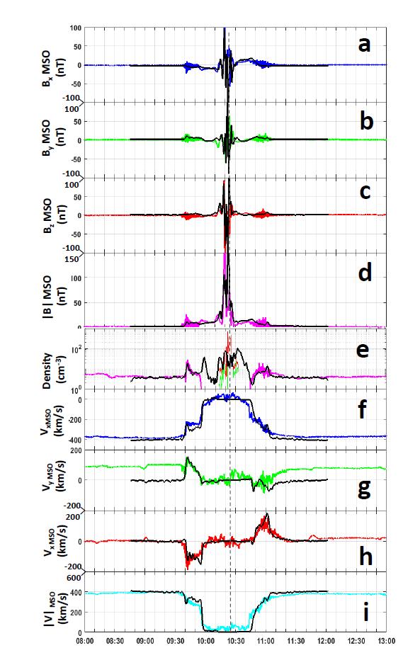
62

63 Figure 10: Comparison between MAVEN measurements between 8h00 and 13h00 on the 07/25/2016 and LatHyS simulation for Table 4 conditions. Solid black lines are for LatHyS simulated results whereas colored lines are for MAVEN measurements. Panel a, b, c and d: Bx, By, Bz and B measured by MAG/MAVEN respectively. Panel e: total electronic density simulated by LatHyS (black), SWIA/MAVEN total ion density (pink), STATIC/MAVEN O + 2 density (red), STATIC/MAVEN O + density (green) in log 10 scale. Panel f, g, h and i: Vx, Vy, Vz, V plasma velocity measured by SWIA/MAVEN respectively. The time of MAVEN closest approach is indicated by the black dashed vertical line.

64 Figure 11: Comparison between MAVEN measurements between 8h00 and 13h00 on the 07/25/2016 and LatHyS simulation for Table 4 conditions. Time energy spectra of the ions, simulated by LatHyS (a), measured by SWIA/MAVEN (b) and by STATIC/MAVEN for all the masses (c). The color scales between panels a, b and c are not similar. The time of MAVEN closest approach is indicated by the black dashed vertical line.

65 Figure 12: Average NGIMS density profiles measured during the period 02/09/2015 to 03/01/2015 (Ls=270 ) on the inbound part of the periapsis path (same density profiles as in Figure 3c) in solid line (same colors as in Figure 3) compared to LMD-GCM and EGM simulated profiles (black star symbols). a: CO 2 density. b: O density. c: N 2 density. d: CO + 2 density. e: O + 2 density.

66 Figure 13: Differential particle flux precipitating into Mars' atmosphere. Panels a, b and c: MAVEN measured flux (blue STATIC ca downward flux, green STATIC d0 downward amu flux, red SWIA downward flux, same as in Figure 4) and simulated precipitating O + ion flux (black line). a: 07/16/ /04/2016. b: 12/13/ /01/2015. c: 02/09/ /27/2015. No crustal field were used in the simulation. Error bars are for the standard deviation of the mean differential measured particle flux. Panels d and e: precipitating flux of O + ion averaged on a 200 km in altitude sphere centered on Mars, panel d: Ls=180 (corresponding to panel a) and panel e: Ls=270 (corresponding to panels b and c).

67 Figure 14: Altitude profile of the nm emission brightness as measured by IUVS/MAVEN (blue lines) and simulated by HELIOSARES (black lines) during the three selected periods (Table 1). Error bars represent the uncertainty on the measurements (black lines).

68 Figure 15: a: Atomic oxygen density (log 10 of O/cm 3 ) in the equatorial plane modeled by EGM using Kharchenko et al. (2000) cross sections. b: Atomic oxygen density (log 10 of O/cm 3 ) in the equatorial plane modeled by EGM using Lewkov and Kharchenko (2014) cross sections. c: IUVS measured brightness intensity of the O nm triplet emission (blue solid line), reconstructed brightness using Kharchenko et al. (2000) cross sections (red solid line) and using Lewkov and Kharchenko (2014) cross sections (black solid line).