Interaction of Two Travelling Wave Solutions of the Non-Linear Euler-Bernoulli Beam Equation

Transcription

1 Interaction of Two Travelling Wave Solutions of the Non-Linear Euler-Bernoulli Beam Equation Shaun Mooney March 26,

2 Contents 1 Introduction 5 2 History of Beam Bending 9 3 Bridges 10 4 LAPACK & CBLAS 13 5 Travelling Waves 16 6 Solitons 19 7 Finite Difference Methods 21 8 Results 31 9 Conclusion 43 References 45 2

3 Abstract We wish to consider the Non-Linear Euler-Bernoulli beam equation, a partial differential that is fourth order in space and second order in time which models the bending of beams. We wish to look at how travelling wave solutions to the aforementioned equation evolve in time and hope to observe that they act in similar way to a set of of partial differential equation known as solitons, that is, upon the interaction of two such solutions, we will see that they emerge relatively unscathed, except for a phase shift. 3

4 Acknowledgements My most sincere thanks must go, first and foremost, to Professor John Stalker. Without his patience, knowledge and guidance this project would not have been completed. My gratitude extends to many other people, not least of whom being Cathal Ó Ruaidh whose brilliant knowledge of both programming and partial differential equations was invaluable. For enlightening me on the history and derivation of the Euler-Bernoulli beam equation I must thank Professor Paschalis Karageorgis. For helping me with gnuplot and C, I would like to thank Louise and Colin, respectively. I would also like to thank the latter for keeping the insanity at bay by writing many brilliant scripts and keeping a pretty decent twitter feed going. 4

5 1 Introduction The Euler-Bernoulli beam partial differential equation is u tt + u xxxx + f (u(x,t)) = 0 (1) where f (u(x,t)) is the non-linearity of the equation. The higher order terms are present because the beam offers resistance to bending. This is how the beam equation differs from, say, that of a vibrating string. If being solved analytically, this equation can be re-written as ρ(x) 2 t 2 u(x,t) + EI(x) 2 This version of the equation is derived in [8]. + f (u(x,t)) = 0 (2) x2 In order to derive equation (1) we need to use Newton s second law of motion and Hooke s law. The former states that force is equal to mass times acceleration, or Force = ma = mu tt An application of Hooke s law states that when an elastic body is deformed in any way the strain is directly proportional to the stress [19]. This can be related to the bending motion using the curvature which can be found by finding the tangential at any point on the beam. This tells us that Force u xxxx, which in turn leads us to equation (1). The first in depth look into this equation was done by Walter and McKenna in 1990 where they used the piece-wise linear model model u tt + u xxxx + u + 1 = 0 This model, however, is not smooth and led to the study of the exponential u tt + u xxxx + e u 1 = 0 5

6 as will be shown later. First, let us consider the piecewise smooth model. We have u tt + u xxxx = cable force where u xxxx is the beam force. We take the deflections of the beam to be in one dimension only, that is, the z direction. In order to obtain the cable force (the non-linearity), we look at Hooke s Law which says that the force is proportional to the displacement of the beam. So k displacement, if u < 0 Force = 0, if u > 0 ku, if u < 0 = 0, if u > 0 = k min(u,0) This leads us to the equation u tt + u xxxx + k min(u,0) = 0 This is called the piecewise linear model and it was studied by McKenna and Walter in [16] and can be rewritten as u tt + u xxxx + u + 1 = 0 This, however, is not a desirable model to use as it has one major drawback: it is not smooth, i.e. it is not differentiable at the origin. So, we require a different model. It is possible to shift figure 1 in order to obtain a more satisfactory non-linear term. It can be shown that figure 2 can be approximated by a smooth function and, therefore, is smooth everywhere. We proceed to look for a factor that has u near the origin and 1 near infinity. A satisfactory function here is f (u) = 1+e u. It is easy to see that as u, f (u) 1. To see an approximation of this function near the origin, we look at 6

7 Figure 1: Piecewise Linear Model of the Euler-Lagrange Beam Equation 7

8 Figure 2: Exponential Model of the Euler-Lagrange Beam Equation the function e x 1 + x. Replacing x with u yields e u 1 u. Rearranging, 1 + e u u. Therefore, which leads to u tt + u xxxx + k[min(u + 1,0)] = 0 u tt + u xxxx + e u 1 = 0 In [13], Karageorgis and McKenna prove ground state solutions exist for this model and allude to the first attempt to solve it numerically by Choi and McKenna, in [6], using the mountain pass theorem. However, they also mention that shooting methods were a faster and more efficient substitute. This idea was explored by Champneys, McKenna and Zegeling in [4]. 8

9 2 History of Beam Bending The problem of beam bending was first considered by Leonardo Da Vinci( ), although he did not have Hooke s Law and was, therefore, not able to do a proper analysis. Da Vinci s work on the subject is described in document called The Codex Madrid [7] which was discovered in 1967[9]. Before The Codex Madrid was found, it was believed that Galileo Galilei( ) was the first to look at the idea of a bending beam. Problems with da Vinci s work, namely his neglection of the strength of the beam and the tensile strength of the material, were addressed by Galileo in his work Dialogues(1638). However, he made incorrect assumptions in his calculations and he got incorrect results. It wasn t until 1713 that Antoine Parent( ) addressed these misguided assumptions in Galileo s work and managed to derive the correct formula for the bending of cantilever beams[10]. In the 18 th century, Charles-Augustin de Coulumb( ) began his work with the theory of beam bending using Parent s conclusions as a basis. He considered how beams made of different materials, like stone and timber, reacted under forces[11]. The vast majority of the work developing a theory for beam bending was done by members of the Bernoulli family and Leonhard Euler( ), who was a student of Daniel Bernoulli. Jacob Bernoulli( ) used infinitesimal calculus to look at deflections in cantilever beams[11]. His nephew, Daniel( ), and Euler did significant work with variational calculus to derive the equations of elastic curves. In 1834 John Scott Russell observed the phenomenon now known as solitons. He observed shallow water waves which we now know can be modelled using the KdV equation. However, the beam equation is also a soliton and, hence, obeys similar laws. Analysis of travelling waves of the Euler-Bernoulli beam equation was begun by Walter and McKenna in 1990[16]. Since then many other mathematicians have tried their hands at these problems and many results have come forth. 9

10 3 Bridges The most common set of examples of the Euler-Bernoulli beam equation in real life are bridges or, more specifically, when bridges collapse. There are many reasons why a bridge could fail (examples include when strong winds blow, people walking, etc.), however, before it does it oscillates wildly. These oscillations are travelling waves. An example of a bridge collapse is the Tacoma Narrows Bridge. 3.1 Tacoma Narrows The Tacoma Narrows Bridge was a suspension bridge built in 1940 in Tacoma, Washington and was first opened to the public in July of that year. It was built to connect the mainland to the Kitsap Peninsula, over the Tacoma Narrows Strait. From the outset, even during construction, it was noticed that the bridge seemed to oscillate when the wind was blowing, even a relatively weak wind (in fact, as a result of the oscillations the locals began calling the bridge Galloping Gertie ). This obviously caused quite a bit of concern with those involved and steps were taken to look for methods of controlling the oscillations at the University of Washington[1]. These precautions included installing hydraulic buffers at the towers in order to control the stresses and, in the side spans tie down cables were installed. However, despite the best efforts of those involved the undulations continued. Even after the bridge was opened and the oscillations continued, the bridge officials refused to close it, despite concerns raised about it s safety. A possible reason for this could be the multitude of people and cars crossing the bridge, all of whom were paying the Toll Authority money, in order to see the amazing moving bridge. It has been noted how cars would seemingly disappear as they drove over it, only adding to spectacle[14]. Not surprisingly, such a structure is clearly not stable and in November 1940, not even five months after it was first opened, the bridge collapsed. In a relatively short time period, the amplitude of the oscillations increased dramatically and became more violent and, eventually, the bridge collapsed due to aeroelastic flutter. Luckily the bridge was free of people when it collapsed, however, tragically, there 10

11 was a car left on it with a dog trapped inside who did not survive. What made the Tacoma Narrows Bridge so famous was that it s catastrophic collapse was caught on camera. Unfortunately, due to the inherent limitations of printed paper, I cannot show said video here. However, if any reader wishes to see it, it is readily available on the internet. Video was taken by four men in total. Two local camera store owners who got wind that the bridge was in a lot of trouble got one video. Barney Elliott stood on the right side, while Harbine Monroe worked from the left. Walter Miles took another video and, finally, so did Professor F. B. Farquharson, which is perhaps the most famous of all.[18] Figure 3: Tacoma Narrows[2] 11

12 Figure 4: The Tacoma Narrows Bridge collapsing[17] 12

13 4 LAPACK & CBLAS LAPACK is a package for numerically solving systems of linear equations. LA- PACK stands for Linear Algebra Package and is ideal for banded, sparse matrices which, as we will see, is exactly what we will be dealing with here. It is a linear algebra library that was written in Fortran 77. As well as analysing and solving systems of equations, LAPACK is also ideal for matrix eigenvalue problems and least square problems. Note that, when using routines, there are four different versions of each routine. These are c, d, s and z. These denote the use of single precision complex points, double precision floating points, single precision floating points and double precision complex points, respectively. The BLAS, which is an acronym for basic linear algebra subprograms, was created in order to make LAPACK more portable and efficient and can be easily optimised for numerous different systems, depending on what the user is running on. It includes many routines to perform linear algebra operations. Like LAPACK, BLAS was originally written for Fortran, with CBLAS being the implementation in C. CBLAS routines are split up into three levels. Level one contains vector-vector operations. Examples of these include scalar addition and multiplication. This is visualised as y αx+y, which is implemented using the command cblas axpy, where is one of c, d, s or z. Also included in level one are dot products, inner products and the ability to copy a vector and swap two vectors, among other operations. Level 2 includes matrix-vector operations. These can be performed on many different types of matrix, including banded, hermitian, packed, symmetric and triangular. Routines such as cblas sbmv multiply a symmetric and banded matrix by a vector, whereas cblas trsv will solve the system of equations Ax = b, where A is a triangular matrix. Level 3 includes matrix-matrix operations. These include operations such as multiplying and adding matrices and solving linear systems. There is also the ability for dealing with the same types of matrices as level 2. 13

14 4.1 Example An example of a program using LAPACK and CBLAS to multiply two matrices is as follows void main(int argc, char **argv) { matrix A, B, C; FILE *afile; FILE *bfile; FILE *cfile; FILE *dfile; afile = fopen("a", "r"); bfile = fopen("b", "r"); cfile = fopen("c", "r"); dfile = fopen("d", "w"); A = readmat(afile, "A", CblasRowMajor); B = readmat(bfile, "B", CblasRowMajor); C = readmat(cfile, "C", CblasRowMajor); ndgemm(cblasrowmajor, CblasNoTrans, CblasNoTrans, 1.0, A, B, 1.0, C); dumpmat(dfile, C, "D", "%7.3f"); } fclose(afile); fclose(bfile); fclose(cfile); fclose(dfile); In this code matrix is a struct which defines a matrix, instead of the usual method of using arrays. The readmat and dumpmat functions read in a matrix from a file and write a matrix to a file, respectively. Of course, there are equivalent usages for vectors and also for dealing with individual entries of matrices and vectors, but I digress. 14

15 The function ndgemm is where the action really happens. This is defined in a wrapper function which calls cblas dgemm from the CBLAS library. This routine multiples a matrix A by a matrix B and then by some constant α. The result of this added to a matrix C multiplied by some constant β. The answer is then stored in C. In shorthand, this routine can be expressed as C αab + βc. Finally, note the use of CblasRowMajor and CblasNoTrans. These are two of the many options that are usable in order to optimise the system that you have to deal with. The former tells CBLAS that we want to use row major matrices instead of column major, which Fortran uses, and the latter tells CBLAS that we do not want to transpose our matrix. Similarly, other routines enable the user to choose between upper and lower triangular matrices and also to decide between left and right multiplication of matrices. Note that there are some restrictions as to what precision points can be used for certain routines. For example, in level 2 operations with symmetric matrices and some matrix updates cannot be used with type c or z. Likewise, operations involving hermitian matrices can only be used with types c and z. The latter is, of course, obvious because hermitian matrices involve complex conjugates, by definition. 15

16 5 Travelling Waves We know that there exist travelling wave solutions to the piecewise linear Euler- Bernoulli beam equation. This was shown by Chen and McKenna[5]. They proved existence of equation (1) with non-linearity f (u) = u + 1. This is the equation that corresponds to a suspended bridge that is a beam supported by cables. Travelling wave solutions are found by setting u = u(x ct) = f (x ct) Computing derivatives of f in x yields f x (x ct) = f (x ct) f xx (x ct) = f (x ct) f xxx (x ct) = f (x ct) f xxxx (x ct) = f (x ct) Computing derivatives of f in t yields f t (x ct) = c f (x ct) f tt (x ct) = c 2 f (x ct) where c is the speed of the wave. We define u u = u x u xx u xxx u x u xx u xxx u = c 2 u xx + e u 1 (3) 16

17 We wish to linearise e u 1, that is to find a linear approximation of the function at u = 0. To do this we use the point-slope formula, i.e. find an equation of the form f (u 2 ) f (u 1 ) = m(u 2 u 1 ) (4) So, we must look for the slope, m, of f (u) = e u 1 at u = 0. The derivative of f with respect to u is f (u) = e u and f (0) = 1. So at u = 0, m = 1, and f (u) = e 0 1 = 0. Subbing into equation (4) gives f (u) = u. Therefore, the linearisation of e u 1 at u = 0 is u. We consider u x u = u xx u xxx c 2 u xx + e u 1 again. Re-writing this in matrix form we get u = A u + B where and A = c B = 0 0 e u 1 u 17

18 is when our travelling wave is at rest. The equation, therefore, written in full matrix form, is u = A u + B u 0 = u x u xx c 2 0 e u 1 u We now have the equation u xxx f iv + c 2 f + e f 1 = 0 where f = f (x ct) Numerical analysis of partial differential equations are notoriously unstable, and this situation is no different. In fact it has been proven by Champneys and McKenna, in [3], that the only stable solutions exist for 0 < c < 2. 18

19 6 Solitons In 1834, a man by the name of John Scott Russell was the first to observe and consider what is now a special set of equations, called solitons. Solitons are special because they are remarkably stable, even under interaction with each other. Whenever one decides to learn about solitons Russell is always mentioned as the first person to observe this phenomenon and, in particular, he is always quoted with the same quote. For reasons of conformity I give this quote here. I also offer it because it is a very good description straight from the horse s mouth[20]: I was observing the motion of a boat which was rapidly drawn along a narrow channel by a pair of horses, when the boat suddenly stopped - not so the mass of water in the channel which it had put in motion; it accumulated round the prow of the vessel in a state of violent agitation, then suddenly leaving it behind, rolled forward with great velocity, assuming the form of a large solitary elevation, a rounded, smooth and well-defined heap of water, which continued its course along the channel apparently without change of form or diminution of speed. I followed it on horseback, and overtook it still rolling on at a rate of some eight or nine miles an hour, preserving its original figure some thirty feet long and a foot to a foot and a half in height. Its height gradually diminished, and after a chase of one or two miles I lost it in the windings of the channel. Such, in the month of August 1834, was my first chance interview with that singular and beautiful phenomenon which I have called the Wave of Translation. It nearly took another fifty years for Russell s observations to be rigorously analysed mathematically and a suitable model found. It wasn t until 1895 that an equation was found to describe the special waves that Russell observed. It was two Dutch mathematicians, Diederik Korteweg and Gustav de Vries, who finally found an equation to describe weakly nonlinear shallow water waves[15]. The Korteweg-de Vries, or KdV, equation is u t + u xxx 6uu x = 0 19

20 A method for finding solutions to this equation and a short discussion of it can be found in [21]. Strauss mentions that the stability properties of the KdV equation were discovered by Kruskal and Zabusky in the 1960s. In fact, the following behaviour can be generalised for all solitons. Upon interaction, two solitons combine in some complicated manner and emerge unscathed except for a phase shift. Since the equation we are dealing with here is also a soliton and, therefore, displays the same kind of behaviour as the KdV equation, we should expect similar results under the interaction of two solutions. 20

21 7 Finite Difference Methods Finite Differences are a popular method to numerically approximate ordinary and partial differential equations. Numerical solvers to these equations are very useful because most of them, especially partial differential equations, either cannot be solved analytically, or they can be solved with great difficulty. There are many reasons why finite difference methods in particular are very popular, not least of which being because they are closely related to the derivative itself. They are formulated by replacing the derivative with a difference equation. We can find an expression for the first derivative of a function, f say, using a Taylor Expansion. Taylor s Theorem states that a k times differentiable function, for k 1, at the point x 0 can be written in the form f (x) = f (x 0 )+ f (x 0 )(x x 0 )+ 1 2 f (x 0 )(x x 0 ) k! f (k) (x 0 )(x x 0 ) k +R k (x 0 )(x x 0 ) k (5) where lim x x0 R k = 0 We can use the above expression in our finite difference method by setting x x 0 = h. Thus, f (x 0 + h) = f (x 0 ) + f (x 0 )h h2 f (x 0 ) + 1 3! h3 f (x 0 ) + = f (x 0 ) + f (x 0 )h + R 1 (x) (6) where R 1 (x) is the remainder term. Rearranging, we find that For sufficiently small R 1 (x), we find that f (x 0 )h = f (x 0 + h) f (x 0 ) R 1 (x) f (x 0 ) = f (x 0 + h) f (x 0 ) R 1 (x) h (7) f (x 0 ) f (x 0 + h) f (x 0 ) h This is called the forward difference of a function, f, and it gives us an approximate solution to the first derivative of that function when h is suitably small, (8) 21

22 i.e. f (x) = lim h 0 f (x + h) f (x) h Note that, as well as forward differences, we can also define central and backward differences. The former are written as f (x) while the latter take the form f (x + h) f (x h) 2h (9) f (x) f (x) f (x h) h (10) Backward difference are derived similarly to forward differences. Instead of getting a Taylor series for f (x + h), we obtain it from This is then rearranged to get (10). f (x h) = f (x 0 ) f (x 0 )h + (11) Equation (9) can be found a number of ways. Adding (8) and (10) gives the result, as does taking an average of our expressions for forward and backward differences. Forward differences effectively describe the slope at a point in terms of the point itself and a point one step-size further along the path. Backward differences calculate the slope using the point itself and the previous point. Central differences don t use the point at which it wants the slope at. Instead it uses the point ahead and behind it. The terms used are clearly very intuitive. We now want to consider this problem on a lattice, which is a mesh of intersecting points where each mesh-point is a point in our finite difference scheme. We will also need to generalise to dimensions, i.e. one temporal and one spatial dimension. This is done easily enough. For the temporal dimension we don t run over step-sizes of the spatial part. All this effectively means is that we replace h by t and introduce an x part. Thus u t = u(t + t,x) u(t,x) t 22

23 Similarly, for the spatial portion we have u x = u(t,x + x) u(t,x) x 7.1 Differences for Higher Order Derivatives As we are dealing with a fourth order differential equation, a first order difference method is clearly not going to be enough. Therefore, we must take this higher, i.e. we need an approximation for the second derivative and an approximation for the fourth derivative. To get an expression for the second derivative we use the Taylor series in two variables, t and x, around t only u(t,x) = u(t 0,x) + u t (t 0,x)(t t 0 ) + u tt (t 0,x)(t t 0 ) 2 + O(t t 0 ) 3 Substituting t t 0 = t into the above equation, we obtain u(t 0 + t,x) = u(t 0,x) + tu t (t 0,x) ( t)2 u tt (t 0,x)(t t 0 ) 2 + O( t) 3 and now substituting in t t 0 = t, we get u(t 0 t,x) = u(t 0,x) tu t (t 0,x) ( t)2 u tt (t 0,x) + O( t) 3 Adding the two above equations yields u(t + t,x) + u(t t,x) = 2u(t,x) + ( t) 2 u tt (t,x) ( t) 2 u tt (t,x) = u(t + t,x) 2u(t,x) + u(t t,x) u tt (t,x) = u(t + t,x) 2u(t,x) + u(t t,x) ( t) 2 Thus, we have an expression for the second derivative of u with respect to t. We can use it to come up with a general expression for the second derivative, i.e. 23

24 2 u = u(t + t,x) 2u(t,x) +U(t t,x) u tt (t,x) = u tt (t,x) = 2 u ( t) 2 u(t + t,x) 2u(t,x) +U(t t,x) ( t) 2 From the definition of the forward difference we have u tt (t,x) = ( ) 2 u = (u(t + t,x) u(t,x)). From [12] we have a general expression for this operator: n u = ( n 1 u) to x Using this we derive an expression for the fourth derivative of u with respect n u(t,x) = ( n 1 u(t,x)) 4 u(t,x) = ( 3 u(t,x)) = ( ( 2 u(t,x))) = ( (u(t,x) 2u(t,x x) + u(t,x 2 x))) = (u(t,x + x) u(t,x) 2u(t,x) + 2u(t,x x) + u(t,x x) u(t,x 2 x)) = (u(t,x + x) 3u(t,x) + 3u(t,x x) u(t,x 2 x)) = u(t,x + 2 x) u(t,x x) 3u(t,x + x) + 3u(t,x) + 3u(t,x) 3u(t,x x) u(t,x x) + u(t,2 x) = u(t,x + 2 x) 4u(t,x + x) + 6u(t,x) 4u(t,x x) + u(t,x 2 x) Therefore, u xxxx (t,x) = u(t,x + 2 x) 4u(t,x + x) + 6u(t,x) 4u(t,x x) + u(t,x 2 x) ( x) 4 24

25 7.2 Reintroducing the equation These approximations can now be plugged into our original partial differential equation u tt + u xxxx + f (u) = 0 u(t + t,x) 2u(t,x) + u(t t,x) ( t) 2 + u(t,x + 2 x) 4u(t,x + x) + 6u(t,x) 4u(t,x x) + u(t,x 2 x) ( x) 4 + f (u(t,x)) = 0 Rewriting the above equation using the substitutions t = m t and x = n x and letting u(m t,n x) = u n (m t), we have u n (t + t) 2u n (t) + u n (t t) ( t) 2 + u n+2(t) 4u n+1 (t) + 6u n (t) 4u n 1 (t) + u n 2 (t) ( x) 4 + f (u n (t)) = 0 u n (t + t) = ( t)2 ( x) 4 ( u n+2(t) + 4u n+1 (t) 6u n (t) + 4u n 1 (t) u n 2 (t)) + 2u n (t) u n (t t) ( t) 2 f (u n (t)) u n (t + t) = ( t)2 ( x) 4 u n 2(t) + 4 ( t)2 ( x) 4 u n+1(t) + (2 6 ( t)2 ( x) 4 )u n(t) + 4 ( t)2 ( x) 4 u n 1(t) t to be ( t)2 ( x) 4 u n 2(t) u n (t t) ( t) 2 f (u n (t)) (12) We define the approximate solution to the partial differential equation at time 25

26 . u n 1 (t) u(t) = u n (t) u n 1 (t). This gives us our solution to the partial differential equation at time t in matrix form. In order to numerically solve for this we must make everything else into matrix form also. This amounts to turning equation (12) into a combination of vectors and matrices. From the definition of u(t) above, u(t + t) and u(t t) can be similarly defined by and. u n 1 (t + t) u(t + t) = u n (t + t) u n 1 (t + t).. u n 1 (t t) u(t t) = u n (t t) u n 1 (t t). We now require a matrix which gives us the same values as equation (12). We can see that this matrix will be symmetric since the coefficient of u n+1 (t) is equal to the coefficient of u n 1 (t) and the coefficient of u n+2 (t) is equal to the coefficient of u n 2 (t), i.e. 4 ( t)2 ( x) 4 and ( t)2 ( x) 4, respectively. Putting this matrix together, and letting ( t)2 ( x) 4 = p, gives 26

27 2 6p 4p p 0 2 6p 4p p 2 6p 4p... where the entries below the diagonal mirror the entries above as the matrix is symmetric. Therefore, our full matrix representation of equation (12) is u(t + t) = Au(t) u(t t) ( t) 2 f (u(t)) p 4p p 0 u n 1 (t + t) 2 6p 4p p u n 1 (t) u n 1 (t t) u n (t + t) = u n 1 (t + t) 2 6p 4p u n (t) u n (t t)... u n 1 (t) u n 1 (t t).... f (u n 1 (t)) ( t) 2 f (u n (t)) f (u n 1 (t)). (13) where f (u)t)) is the non-linear term. Notice that, in the above equation, we have three unknown temporal values of u, namely t t, t and t + t. Since we only have one initial value we need to eliminate one of these. To do this we use the calculus of finite differences as outlined by Strikwerda in [22]. We want to look at a central difference. By the Taylor series, we have u(x + h) = h i i=0 i! i u(x) = e h This leads to the following expression for the forward difference 27

28 e hd 1 h and the backward difference can be written as where D is the differential operator. 1 e hd h Thus, combining the two equations above we find that the central difference can be expressed By the Taylor series we have = 1 ( e hd ) e hd 2 h h = ehd e hd 2h = sinh(hd) h D = arcsinh(h ) h D = h 1 6 (h )3 h u x (t,x) = 1 6 h2 ( ) 3 We are looking for a derivative in t, so we must find some relation between u x and u t. Since our solutions are travelling waves we can look u(t,x) = f (x ct). Differentiating we find that where c is the speed of our wave. Taking h = x, we get u t = c u x 28

29 u t (t,x) = cu x (t,x) ( ) u(t,x + x) u(t,x x) = c 2 x ( + c 1 6 ( = c 1 12 x u t (0,x) = c = c ( 1 u(t,x + 2 x) 2u(t,x + x) + 2u(t,x x) u(x,t 2 x 2 x u(t,x + 2 x) + u(t,x + x) u(t,x x) + u(t,x 2 x) 3 x 3 x 12 x u(0,x + 2 x) + u(0,x + x) u(0,x x) + 3 x 3 x 12 x 12 x ( u(0,x + 2 x) u(0,x + x) + u(0,x x) 12 x 3 x 3 x As before, this can be represented in matrix notation and calculated numerically. Explicitly, t = c x 0 3 x 2 c 1 12 x x c x 12 x 12 x 1 c 2 3 x c 0 3 x ) ) ) u(0,x 2 x) ) u(0,x 2 x) 12 x (14) (15) We are now able to calculate the first time step. To do this we consider our finite difference scheme at t = 0, u( t,x) + u( t,x) = Au(0,x) ( t) 2 f (u(0,x)) (16) and a finite difference for the first derivative of t, u( t,x) u( t,x) = 2 tu t (0,x) (17) Adding equations (16) and (17) we get 2u( t,x) = Au(0,x) ( t) 2 f (u(0,x)) + 2 tu t (0,x) u( t,x) = 1 2 Au(0,x) 1 2 t)2 f (u(0,x)) + tu t (0,x) 29

30 and we can now use this to find further temporal values. An important aspect of these calculations is the correct choice of t and x. The initial data I am using was generated on an interval of [ 60,60] over a beam of length 600 so, therefore, we have x = 1 5 = 0.2. What we must now do is choose a time step which will make sure that the travelling wave remains stable. The stability condition we use, which comes from [4], is t ( x) t t 1 50 (18) In order to satisfy this inequality, choose t = 80 1 = We now have a finite difference scheme with the stability condition satisfied. It should be clear that the bulk of the work takes place using this finite difference model. However, to hard code this would be relatively difficult. This is where LAPACK and CBLAS routines come into their own. They make coding linear algebra exceptionally easy. To illustrate this, I present my code that runs inside a for-loop and is the most important part of the code. ndsbmv(cblasrowmajor, CblasUpper, 1.0, sybify(a, 2), x, -1.0, y); ndaxpyv(-dt*dt, z, y); This is incredibly simple code that performs some not-so-simple computations. The first line of the code calls the CBLAS routine cblas dsbmv, which takes a symmetric and banded matrix, A, of band width 2, multiplies it by a vector x and then subtracts a vector y. The vector y is then replaced with the answer. The second function calls the CBLAS routine cblas daxpy which adds the vector y to ( t) 2 times z. The vector z here is, of course, the non-linearity term in our partial differential equation. This quick illustration shows just how useful implementations such as LA- PACK and CBLAS really are and how much they simplify the coding process. 30

31 8 Results The idea of this project is to look at the interaction of two solutions. Therefore, we need two solutions with which to propagate over time. These two solutions are travelling waves and differ only in that they have been generated using different speeds. The first one was computed taking c 2 = 1 and is shown in figure 5. Figure 5: solution with c 2 = 1 The second solution has been generated with c 2 = 0.25 and can be seen in figure 6. 31

32 Figure 6: solution with c 2 = 0.25 We now want to look at how these interact with each other. Positioning each one at either end of our beam, as in figure 7, we wish for them to move towards each other. 32

33 Figure 7: A solution with c = 0.5 on the left and a solution with c = 1 on the right Evolving this system in time, we get the following results: 33

34 34

35 35

36 In order to demonstrate the stability condition given in equation (18), we will look at what happens to a wave that doesn t satisfy this t 1 Taking t = 25 1, we find that the wave with c = 1 behaves as follows

37 Figure 8: An unstable solution with c = 1 37

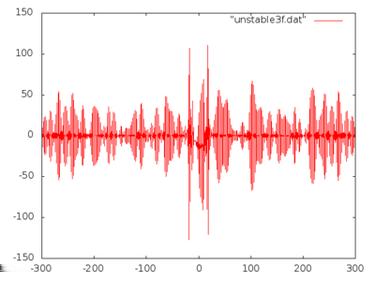
38 38

39 This solution is clearly very unstable and blows up after a very short amount of time. We have already looked at what happens when two solitons moving in opposite directions interact. Now let us consider two solitons moving in the same direction. This time we begin with both waves on the same side of the beam, the slower one in front of the faster one, and we carry out the same experiment as before. 39

40 40

41 41

42 As we can see, these interactions are remarkably stable, with the each wave emerging intact except for a phase shift. As well as the Euler-Bernoulli beam equation, there are many other equations that show these same properties. Some examples of these, that is partial differential equations with soliton solutions, include the aforementioned KdV equation, the Non-Linear Shrödinger equation and the Sine-Gordon equation. 42

43 9 Conclusion Since the first observation of solitons by Russell in 1834, they have been studied by a great many people. Their stability properties have been well documented and, in this paper, we see them again. We have seen, by numerically solving the Euler-Bernoulli beam equation using the finite difference method, that these stability properties do in fact hold and, furthermore, that they are even stable under interaction with each other. This finite difference method was implemented with matrix notation by using a package to deal with linear algebra called LAPACK and was supplemented with another package called CBLAS. A travelling wave solution was fired along a beam and shown to display the desirable stability properties. We have seen that this stability holds for waves moving in opposite directions and also for waves moving in the same direction. The stability property used was equation (18), given in [4]. We have also seen that violating this stability causes the wave to oscillate wildly and, eventually, blow up. 43

44 References [1] Tacoma narrows [2] Tacoma narrows picture [3] A. R. Champneys and P. J. McKenna. On solitary waves of a piecewise linear suspended beam model. Nonlinearity, 10(6): , [4] A. R. Champneys, P. J. McKenna, and P. A. Zegeling. Solitary waves in nonlinear beam equations: stability, fission and fusion. Nonlinear Dynam., 21(1):31 53, The theme of solitary waves and localization phenomena in elastic structures. [5] Y. Chen and P. J. McKenna. Traveling waves in a nonlinearly suspended beam: theoretical results and numerical observations. J. Differential Equations, 136(2): , [6] Y. S. Choi and P. J. McKenna. A mountain pass method for the numerical solution of semilinear elliptic problems. Nonlinear Anal., 20(4): , February [7] Leonardo Da Vinci. The Codex Madrid. Natioanl Library of Spain, [8] Bill Goodwine. Engineering Differential Equations: Theory & Applications. Springer. [9] Doug Jeknins. The History of the Theory of Beam Bending - Part 1@ON- LINE. [10] Doug Jeknins. The History of the Theory of Beam Bending - Part 2@ON- LINE. [11] Doug Jeknins. The History of the Theory of Beam Bending - Part 3@ON- LINE. [12] Charles Jordan. Calculus of Finite Differences. Chelsea Publishing Company New York, N.Y.,

45 [13] Paschalis Karageorgis and P. J. McKenna. The existence of ground states for fourth-order wave equations. Nonlinear Anal., 73(2): , [14] Mark Ketchum. A short history of galloping [15] Mathworld. Korteweg-de vries equation@online. [16] P. J. McKenna and W. Walter. Travelling waves in a suspension bridge. SIAM J. Appl. Math., 50(3): , [17] npr. Tacoma narrows picture 2@ONLINE. [18] Washington State Dept. of Transportation. Tacoma narrows bridge@online. [19] B. Pearson. Deflection of a beam - young s modulus@online. [20] John Scott Russell. Report On Waves. British Association, [21] Walter Strauss. Partial Differential Equations: An Introduction. Wiley. [22] John Strikwerda. Finite Differentaik Schemes and Partial Differential Equations. Siam. 45