Modern Methods of Statistical Learning sf2935 Lecture 5: Logistic Regression T.K

Transcription

1 Lecture 5: Logistic Regression T.K

2 Overview of the Lecture

3 Your Learning Outcomes Discriminative v.s. Generative Odds, Odds Ratio, Logit function, Logistic function Logistic regression definition likelihood function: perfect linear classifier as special case maximum likelihood estimate best prediction and linear perceptron Accuracy, Precision, Sensitivity, Specificity

4 The setting: Y is a binary r.v.. x is its covariant, predictor or explanatory variable. x can be continuous, categorical. We cannot model the assocication of Y to x by a direct linear regression, Y = α + βx + e where e is, e.g., N (0, σ 2 ). Y = Bacterial Meningitis or Acute Viral Meningitis. x =cerebrospinal fluid total protein count.

5 Logistic regression Let x i X R p, y i Y = {+1, 1} 1, X = (X 1,..., X p ) T, a vector. Y is r.v. with two values, 1 and 1. We consider the problem of modelling the probability P (Y = 1 X). The model will be called logistic regression. 1 We could use Y = {+1, 0}

6 Supervised Learning Let x i X R p, y i Y = {+1, 1}, i = 1,... n be n pairs of examples of a binary target concept. Then is the training set. S = {(x 1, y 1 ),..., (x n, y n )} Training logistic regression using S, prediction of Y using x X and logistic regression. P (Y = 1 X) We need some additional concepts.

7 Supervised Learning; Supervised Classification Modelling of P (Y = 1 X) This is known as the discriminative approach to supervised classification (with binary alternatives). The generative approach: Model P (X Y = 1) and P (Y = 1) and use Bayes, formula to find P (Y = 1 X). The discriminative approach models P (X Y = 1) and P (Y = 1) and implicitly. There is an Appendix showing how a certain generative model of binary classification can be transformed to a logistic regression.

8 Generative: Class Data Discriminative: Data Class

9 Part I: Concepts Odds, Odds Ratio Logit function Logistic function a.k.a Sigmoid function

10 Odds The odds of a statement (event e.t.c) A is calculated as the probability p(a) of observing A divided by the probability of not observing A: odds of A = p(a) 1 p(a) E.g., in humans an average of 51 boys are born in every 1000 births, the odds of a randomly chosen delivery being boy are: odds of a boy = = 1.04 The odds of a certain thing happening are infinite.

11 An Aside: Posterior Odds The posterior probability p(h E ) of H given the evidence E: posterior odds of H = p(h E ) 1 p(h E ) If there are only two alternative hypotheses, H and not-h, then posterior odds of H = p(h E ) p(not-h E ) by Bayes formula = p(e H) p(h) p(e not-h) p(not-h). = likelihood ratio prior odds

12 Odds ratio The odds ratio ψ is the ratio of odds from two different conditions or populations. ψ = odds of A 1 odds of A 2 = p(a 1 ) 1 p(a 1 ) p(a 2 ) 1 p(a 2 )

13 Bernoulli Distribution again Consider r.v. Y with values 0, 1, 0 < p < 1 and y = 1 y = 0 f (y) p 1 p Y Be(p) = Bin(1, p).

14 Bernoulli Distribution again We write this as and y = 1 y = 0 f (y) p 1 p f (y) = p y (1 p) 1 y = e ln( p 1 p )y+ln(1 p)

15 The function logit(p) The logarithmic odds of success is called the logit of p ( ) p logit(p) = ln 1 p f (y) = e ln( p 1 p )y+ln(1 p) = e logit(p)y+ln(1 p)

16 The function logit(p) and its inverse ( ) p logit(p) = log 1 p If θ = logit(p), then the inverse function is p = logit 1 (θ) = eθ 1 + e θ

17 The logit(p) and its inverse The function ( ) p logit(p) = log, 0 < p < 1 1 p p = logit 1 (θ) = σ(θ) = eθ 1 + e θ = e θ 1, < θ <, 1 + e θ is called the logistic function or sigmoid. Note that σ(0) = 1 2.

18 Logistic function a.k.a. sigmoid In biology the logistic function refers to change in size of a species population. In artifical neural networks it is a network output function (sigmoid). In statistics it is the canonical link function for the Bernoulli distribution (c.f. above).

19 The logit(p) and the logistic function Sats The logit function ( ) p θ = logit(p) = log, 0 < p < 1 1 p and the logistic function p = σ(θ) = are inverse functions to each other. 1, < θ <, 1 + e θ

20 The logit(p) and the logistic function ( ) p 1 θ = logit(p) = log, 0 < p < 1 p = σ(θ) =, < θ <, 1 p 1 + e θ

21 Part II: Logistic Regression A regression function log odds of Y a regression function How to generate Y, logistic noise

22 Let β = (β 0, β 1, β 2,..., β p ) be (p + 1) 1 vector and X = (1, X 1, X 2,..., X p ) be a (p + 1) 1 -vector of (predictor) variables. We set, as in multiple regression, β T X = β 0 + β 1 X 1 + β 2 X β p X p Then G (X) = σ(β T X) = T X e = e β βt X 1 + e βt X

23 Logistic regression The predictor variables (X 1, X 2,..., X p ) can be binary, ordinal, categorical or continuous. In the examples below they are mostly continuous.

24 e βt X G (X) = σ(β T X) = 1 + e βt X By construction 0 < G (X) < 1. Then logit is well defined and logit(g (X)) = ln G (X) 1 G (X) = βt X = β 0 + β 1 X 1 + β 2 X β p X p.

25 Logistic regression Let now Y be a binary random variable such that { 1 with probability G (X) Y = 1 with probability 1 G (X) Definition If the logit of G (X) (or log odds of Y ) is logit(g (X)) = ln G (X) 1 G (X) = β 0 + β 1 X 1 + β 2 X β p X p, then we say that Y follows a logistic regression w.r.t. the predictor variables X = (1, X 1, X 2,..., X p ).

26 Logistic regression For fixed β we have the hyperplane D(β) = {X β T X = 0} For any X D(β), G (X) = σ(0) = 1 2 and Y = { 1 with probability with probability 1 2

27 An Aside: Deciban We might use (suggestion by Alan Turing for logarithm of posterior odds) e(y X) = 10 log 10 G (X) 1 G (X) and call it the evidence for Y given X. Turing called this deciban. The unit of evidence is then decibel (db). 1 db change in evidence is the smallest increment in of plausibility that is perceptible for our intuition.

28 Logistic regression: genetic epidemiology Logistic regression { success with probability G (X) Y = failure with probability 1 G (X) logit(g (X)) = ln G (X) 1 G (X) = β 0 + β 1 X 1 + β 2 X β p X p. is extensively applied in medical research, where success may mean the occurrence of a disease or death due to a disease, and X 1, X 2,..., X p are environmental and genetic riskfactors. Woodward, M. : Epidemiology: study design and data analysis, 2013, CRC Press.

29 Logistic regression: genetic epidemiology Suppose we have two populations, where X i = x 1 in first population and X i = x 2 in the second population, all other predictors are equal in the two populations. Then a medical geneticist finds it useful to calculate the logarithm of the odds ratio ln ψ = ln p 1 1 p 1 ln = β i (x 1 x 2 ) p 2 1 p 2 or ψ = e β i (x 1 x 2 )

30 EGAT Study (from Woodward) Smoker at entry Cardiovascular death during follow-up Yes No Total Yes No Total

31 EGAT Study (from Woodward) Logistic regression logit = x was fitted with x = 1 for smokers and x = 0 for non-smokers. Then the odds ratio is The log odds for smokers is ψ = e β(x 1 x 2 ) = e (1 0) = = giving odds= For non-smokers the odds are

32 EGAT Study (from Woodward) The risk for cardiovascular death for smokers is 1 = e For nonsmokers 1 = e

33 Logistic regression e βt X P(Y = 1 X) = G (X) = σ(β T X) = 1 + e βt X 1 P(Y = 1 X) = 1 G (X) = e = e β βt X 1 + e βt X = e βt X. Hence a unit change in X i corresponds to e β i change in odds and β i change in logodds. T X

34 ɛ is a r.v., ɛ Logistic(0, 1) means that the cumulative distribution function (CDF) of the logistic distribution is the logistic function: P (ɛ x) = 1 = σ(x) 1 + e x

35 A generative model We need the following regression model Y = β T X + ɛ where β T X = β 0 + β 1 X 1 + β 2 X β p X p and ɛ Logistic(0, 1), i.e. the variable Y can be written directly in terms of the linear predictor function and an additive random error variable. The logistic distribution (?) is the probability distribution the random error.

36 Logistic distribution ɛ is a r.v., ɛ Logistic(0, 1) means that the cumulative distribution function (CDF) of the logistic distribution is the logistic function: P (ɛ x) = 1 = σ(x) 1 + e x I.e. ɛ Logistic(0, 1), if the probability density function is d dx σ(x) = e x (1 + e x ) 2.

37 Simulating ɛ Logistic(0, 1) This is simple: simulate p 1,..., p n from the uniform distribution on (0, 1) and then do ɛ i = logit(p i ), i = 1,..., n. In the figure we plot the empirical distribution function of ɛ i for n =

38 A piece of probability ɛ Logistic(0, 1), what is P ( ɛ x)? P ( ɛ x) = P (ɛ x) = 1 P (ɛ x) = 1 σ( x) = e x = ex 1 + e x = e x = P (ɛ x). ɛ Logistic(0, 1) ɛ Logistic(0, 1).

39 Generating model and/or how to simulate Take a continuous latent variable Y (latent= an unobserved random variable) that is given as follows: Y = β T X + ɛ where β T X = β 0 + β 1 X 1 + β 2 X β p X p and ɛ Logistic(0, 1).

40 Define the response Y as the indicator for whether the latent variable is positive: { 1 if Y > 0 i.e. ε < β T X, Y = 1 otherwise. Then Y follows a logistic regression w.r.t. X. We need only to verify that 1 P(Y = 1 X) = 1 + e. βt X

41 P(Y = 1 X) = P(Y > 0 X) (1) = P(β T X + ε > 0) (2) = P(ε > β T X) (3) = P( ε < β T X) (4) = P(ε < β T X) (5) = σ(β T X) (6) 1 = (7) 1 + e βt X where we used in (4) -(5) that the logistic distribution is symmetric (and continuous), as learned above, Pr ( ε x) = Pr (ε x).

42 Part III: Logistic Regression Simulated Data Some Probit Analysis Maximum Likelihood

43 Simulate ɛ, compute Y = β T X + ɛ with known β and levels of X. Compute { 1 if Y > 0 i.e. ε < β T X, Y = 0 otherwise.

44 Maximum likelihood We have data S = {(X 1, y 1 ),..., (X n, y n )} Next the labels are coded as +1 +1, 1 0. The likelihood function is L (β) def = l i=1 G (X i ) y i (1 G (X i )) 1 y i.

45 Maximum likelihood Some simple manipulation gives that ln L (β) = n i=1 ( )) y i β T X i ln (1 + e βt X i There is no closed form solution to the minimization of ln L (β). The function is twice continuously differentiable, convex and even strictly convex if the data is not linearly separable (c.f., sf2935 Lecture 1). There are standard optimization algorithms for minimization of functions with these properties.

46 Model validation: the χ 2 -test Let us look at following data on dose pesticide and death. We can write the data for males as Dose (µg) Die Survive

47 Model validation: the χ 2 -test Using the ML-estimates α = and β = we can calculate the probability of death for the dose x = 1 as 1 = e and then the expected frequency of death at x = 1 is = In the same way we can calculate the probabilities of death and survival for the other doses x.

48 Model validation: the χ 2 -test We use the chi-square goodness-of-fit test statistic Q Q = r (observed freq i expected freq i ) 2 r (x = i np i ) i=1 expected freq 2. i i=1 np i where r is the number of groups in the grouped data. It can be shown that Q is approximatively χ 2 (r/2 2)- distributed (chi square with r/2 2 degrees of freedom) under the (null) hypothesis that the probabilities of death and survival are as given by the estimated model. The reduction with two degrees of freedom is for the fact that we have estimated two parameters.

49 Model validation: the χ 2 -test Q = r (observed freq i expected freq i ) 2 r (x = i np i ) i=1 expected freq 2. i i=1 np i E.g., n 2 = 4 and n p 2 = 20 P(Y = 1 x = 2) = e α 2 β

50 Model validation: the χ 2 -test We get Q = 12 (observed freq i expected freq i ) 2 i=1 expected freq i ( )2 ( )2 = = The p-value is P (Q 4.24) = where Q is χ 2 (6 2)- distributed. Hence we do not reject the logistic regression model 2. 2 Here the expected frequency of 0 taken as 0.01 in the textbook cited.

51 Part IV: More on Maximum Likelihood Likelihood function rewritten Training: an algorithm for computing the Maximum Likelihood Estimate Linear Separability and Regularization

52 Part V: Logistic Regression Special case: β T X = β 0 + β 1 x. Likelihood Maximum Likelihood

53 We consider the model: β T X = β 0 + β 1 x. P(Y = 1 x) = σ(β T X) = e (β 0+β 1 x)

54 Notation: P(Y = y x) = σ(β T X) y (1 σ(β T X) 1 y = { σ(β T X) if y = 1 1 σ(β T X) if y = 0

55 Data (x i, y i ) n i=1, likelihood function with the notation above L (β 0, β 1 ) = P(Y = y 1 x 1 ) P(Y = y 2 x 2 ) P(Y = y n x n ) = σ(β T X 1 ) y 1 (1 σ(β T X 1 ) 1 y1 σ(β T X n ) y n (1 σ(β T X n ) 1 y n = A B A = σ(β T X 1 ) y1 σ(β T X 2 ) y2 σ(β T X n ) y n B = (1 σ(β T X 1 ) 1 y 1 (1 σ(β T X 2 ) 1 y2 (1 σ(β T X n ) 1 y n

56 = n i=1 + ln L (β 0, β 1 ) = ln A + ln B n i=1 = n y l ln σ(β T X i ) i=1 (1 y i ) ln(1 σ(β T X i )) ln(1 σ(β T X i )) + n i=1 σ(β T X i ) y l ln 1 σ(β T X i )

57 ( ln(1 σ(β T X i )) = ln 1 ( e (β 0+β 1 x) = ln 1 + e (β 0+β 1 x i ) ( ) 1 = ln 1 + e β 0+β 1 = x i ) = ln (e β 0+β 1 x i ) e (β 0+β 1 x i ) )

58 logodds σ(β T X i ) ln 1 σ(β T X i ) = β 0 + β 1 x i

59 In summary: ln L (β 0, β 1 ) = n i=1 y i (β 0 + β 1 x i ) n i=1 ) ln (e β 0+β 1 x i

60 = n i=1 β 1 ln L (β 0, β 1 ) y i x i n i=1 ) ln (e β 0+β 1 x i β 1 ) ln (e β 0+β 1 x i β 1 = e β 0+β 1 x i x i 1 + e β 0+β 1 x i = P(Y = 1 x i ) x i.

61 ln L (β 0, β 1 ) = 0 β 1 n (y i x i P(Y = 1 x i ) x i ) = 0. i=1 In the same manner we can also find n ln L (β 0, β 1 ) = β 0 (y i P(Y = 1 x i )) = 0 i=1 These two equations have no closed form solution w.r.t. β 0 and β 1.

62 Newton-Raphson for MLE: a one-parameter case For one parameter θ, set f (θ) = ln L(θ). We are searching for the solution of Newton-Raphson method f (θ) = d f (θ) = 0. dθ θ new = θ old + f ( θ old ) where a good initial value is desired. f (θ old ),

63 Newton-Raphson for logistic MLE ( β new 0 β new 1 ) = ( β old 0 β old 1 ) ( + H 1 (β old 0, β old β 1 ) 0 ln L ( β old 0, ) βold 1 β 1 ln L ( β old 0, ) βold 1 ). where H 1 (β old (next slide) 0, βold 1 ) is the matrix inverse of the 2 2 matrix

64 Newton-Raphson for logistic MLE H(β old 0, β old 1 ) = 2 β 2 0 ln L ( β old 0, ) βold 1 2 β 1 β 0 ln L ( β old 0, βold 1 ) 2 β 0 β 1 ln L ( β old 2 β 2 1 0, βold 1 ln L ( β old 0, βold 1 ) ) = n i=1 P (Y = 1 x i ) (1 P(Y = 1 x i ) n i=1 P (Y = 1 x i ) (1 P(Y = 1 x i ) right)cdotx i n i=1 P (Y = 1 x i ) (1 P (Y = 1 x i )) x i n i=1 P (Y = 1 x i ) (1 P(Y = 1 x i )) x 2 i

65

66 The trick applied to rewriting the logistic probability σ(t) = e t Let us recode y {+1, 1}. Then we get ( ) P (y X) = σ y β T X

67 Logistic Regression: a check y {+1, 1}. P (+1 X) = σ(t) = e t 1 ( ) 1 + e = σ +1β T X. βt X 1 P ( 1 X) = 1 P (+1 X) = e βt X = e βt X 1 + e βt X = e βt X 1 + e = 1 ( ) βt X e βt X + 1 = σ 1β T X.

68 Logistic Regression: Likelihood of β A training set The likelihood function of β is ( ) P (y X; β) = σ y β T X S = {(X 1, y 1 ),..., (X n, y n )} L (β) def = n i=1 P (y l X l ; β)

69 Logistic Regression: -log likelihood of β The negative log likelihood l (β) def = ln L (β) = n = ln P (y l X l ; β) i=1 n ) = ln σ (y i β T X i i=1 = n ln i=1 = n ln i=1 [ e y i β T X i ] [1 + e y i β T X i ]

70 Logistic Regression: ML (1) Let us recall that l (β) = n ] ln [1 + e y i β T X i i=1 β = (β 0, β 1, β 2,..., β p ). Then ] ln [1 + e y i β T X i e y i(β T X i) = y i β e y i β T X i = y i σ( y i β T X i ) = y i (1 P (y i X; β))

71 Logistic Regression: ML (2) l (β) = n ] ln [1 + e y i β T X i i=1 β = (β 0, β 1, β 2,..., β p ). ] ln [1 + e y i β T X i e y i(β T X i) = y i X i β k 1 + e y i β T X i = y i X i σ( y i β T X i ) = y i X i (1 P (y i X; β))

72 Logistic Regression: ML (3) l (β) = β = (β 0, β 1, β 2,..., β p ). n ] ln [1 + e y i β T X i i=1 ] ln [1 + e y i β T X i = y i (1 P (y i X; β)) β 0 ] ln [1 + e y i β T X i = y i X i (1 P (y i X; β)) β k

73 Logistic Regression: ML (3) Update ] ln [1 + e y i β T X i = y i (1 P (y i X; β)) β 0 ] ln [1 + e y i β T X i = y i X i (1 P (y i X; β)) β k Parameters can then be updated by selecting training samples at random and moving the parameters in the opposite direction of the partial derivatives (stochastic gradient algorithm).

74 Logistic Regression: ML (4) Update Parameters can then be updated by selecting training samples at random and moving the parameters in the opposite direction of the partial derivatives β 0 β 0 + ηy i (1 P (y i X; β)) β β + ηy i X i (1 P (y i X; β))

75 Logistic Regression: ML (5) Update β 0 β 0 + ηy i (1 P (y i X; β)) β β + ηy i X i (1 P (y i X; β)). Resembles strongly of the perceptron algorithm, with on-line updates driven by mistakes. The difference here is that the updates are made in proportion to the probability of making a mistake. We give no proof of convergence.

76 Properties of ML Assume that the training examples S = {(X 1, y 1 ),..., (X n, y n )} is linearly separable (c.f., Lecture I). In this case we know (previous lecture) that the are values of β such that y i β T X i > 0 for all training examples. Then the likelihood function L (β) = n i=1 ) σ (y i β T X i = n i= e y i β T X i is strictly increasing as a function of y i β T X i. Hence we can scale up 3 the parameters β and make them larger and larger. Thus the maximum likelihood estimated values increase to infinity for a perfect linear classifier. 3 Scaling freedom of Lecture I

77 ML & Regularizer To avoid linear separability due to small training sets we minimize the regularizer + the negative loglikelihood function or λ 2 βt β + n i=1 ] ln [1 + e y i β T X i where λ is a parameter that measures the strength of regularization.

78 More on ML n ) l (β) = ln σ (y i β T X i i=1 Then we recall that X = (1, X 1, X 2,..., X p ). Thus l β F (β) = y i X i σ( y i β T X i ). i=1 This follows by the preceding, or expressing the preceding in vector notation β βt X = β XT β = X Thus if we set the gradient βf (β) = 0 (= a column vector of p + 1 zeros) we get n y i X i σ( y i β T X i ) = 0 i=1

79 The ML estimate β will satisfy 0 = 0 = n y i σ( y i βt Xi )X i i=1 n y i (1 P(y i βt Xi )X i i=1

80 The section above is partially based on: T.S. Jaakkola: course material for Machine Learning, Fall 2006, MIT, T.S. Jaakkola & D. Haussler (1998): Exploiting generative models in discriminative classifiers. T.S. Jaakkola & D. Haussler (1999): Probabilistic kernel regression models. Proceedings of the Seventh International Workshop on Artificial Intelligence and Statistics.

81 Part IV: Prediction Prediction & Perceptron Crossvalidation

82 When we insert β back to P (y X) we have ( P (y X) = σ y β T ) X or ) P (Y = 1 X) = σ ( βt X

83 Logistic Regression as Perceptron We can drop the notations P and β for ease ( of writing. ) For given X the task is to maximize P (y X) = σ y β T X. There are only two values y = ±1 to choose among. There are two cases to consider. 1) t = β T X > 0. Then if y = +1, and y = 1 y t < 0 < yt e y t < e yt e yt < e y t i.e. 1 + e yt < 1 + e y t e y t < e yt P (y X) = σ (yt) > σ (y t) = P (y X)

84 Logistic Regression as Perceptron 2) t = β T X < 0. If y = +1, and y = 1, then yt < y t and it follows in the same way as above that P (y X) > P (y X) Hence: the maximum probability is assumed by y that has the same sign as β T X.

85 Logistic Regression as Perceptron Given β, the best probability predictor of Y, denoted by Ŷ, for given X is ) Ŷ = sign ( β T X This is recognized as the input-output map of a perceptron, c.f., Lecture I. The training of logistic regression is not, however, done by the perceptron algorithm.

86 Model validation: Cross-validation A way to check a model s suitability is to assess the model against a set of data (testing set) that was not used to create the model: this is called cross-validation. This is a holdout model assessment method.

87 Cross validation We have a training set of l pairs Y {0, 1} and the corresponding values of the predictors. S = {(X 1, y 1 ),..., (X n, y n )} and use this to estimate β by β = β(s), e.g., by ML. We must have another set of data, testing set, of holdout samples T = {( X t 1, y1) t (,..., X t m, ym t )} Having found β we should apply the optimal predictor P (y X t l ) on T, and compare the prediction to yj t for all j. Note that in this β = β(s)

88 Cross-validation: categories of error prediction of -1 when the holdout sample has a -1 (True Negatives, the number of which is TN) prediction of -1 when the holdout sample has a 1 (False Negatives, the number of which is FN) prediction of 1 when the holdout sample has a -1 (False Positives, the number of which is FP) prediction of 1 when the holdout sample has a 1 (True Positives, the number of which is TP)

89 Evaluation of logistic regression (and other) models False Positives = FP, True Positives = TP False Negatives = FN, True Negatives= TN Y = +1 Y = 1 Ŷ = +1 TP FP Ŷ = 1 FN TN

90 Cross-validation In machine learning & medical research one often encounters one or several of the following criteria of evaluating a classifier: TP+TN Accuracy = TP+FP+FN+TN =fraction of observations with correct predicted classification Precision = PositivePredictiveValue = predicted positives that are correct TP TP TP+FP =Fraction of Recall = Sensitivity = TP+FN =fraction of observations that are actually 1 with a correct predicted classification TN Specificity = TN+FP =fraction of observations that are actually -1 with a correct predicted classification

91 Simulated Data The same as above: With the true generative model log(p/(1 p)) = x + ɛ, we simulate 2000 pairs of test data. We predict Y in the test set using α = 3.21, β = found from the training data. The results are: Accuracy = Precision= Recall=Sensitivity= Specificity= Negative Predictive value=

92 Error rates with statistics names Let N=TN+FP, P=FN+TP. FP/N = type I error = = 1 Specificity TP/P= 1-type II error = =power =sensitivity=recall

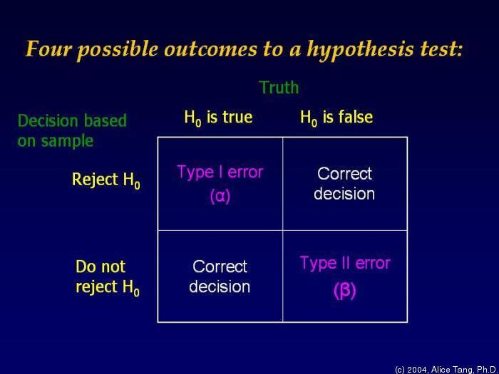
93 Hypothesis testing

94 Hypothesis testing