Basic Statistics. Resources. Statistical Tables Murdoch & Barnes. Scientific Calculator. Minitab 17.

Transcription

1 Basic Statistics Resources 1160 Statistical Tables Murdoch & Barnes Scientific Calculator Minitab

2 Statistics 1161 The science of collection, analysis, interpretation and presentation of data in the best way possible The science of making decisions in the face of uncertainty The following measurements, in mg, represent observations obtained from analysis of a chemical process: 21, 20, 20, 19, 21, 22, 20, 18, 19, 20, 18 Analyse this data. General Concepts and Definitions 1162 What Is A Sample? A finite sub-set of observations deemed to be representative of the set of all possible outcomes What Is A Population? The set of all possible outcomes, eg a production run, output of one shift etc 2

3 General Concepts and Definitions 1163 What Is A Statistic? A characteristic of the sample such as sample average, standard deviation, variance etc What Is A Parameter? A characteristic of the population such as population mean General Concepts and Definitions 1164 Statistical Process Control (SPC) Application of statistical methods to monitor, analyse and control process variability Controlling process variability ensures that it operates at its full potential 3

4 General Concepts and Definitions 1165 Key statistical indices Obtained from Sample Obtained from Population Individual value x x Mean μ Variance s 2 σ 2 Standard Deviation s σ Measures of Central Tendency 1166 Median The middle observation when a set of data is ordered in ascending or descending order Mode The most frequently occurring observation Minitab Stat Basic Statistics Display Basic Statistics 4

5 Measures of Central Tendency 1167 Mean Arithmetic average of a set of observations 21, 20, 20, 19, 21, 22, 20, 18, 19, 20, 18 18, 18, 19, 19, 20, 20, 20, 20, 21, 21, 22 Measures of Dispersion Variance 1168 A measure of the variability in the data, based on the squared deviations from the mean Standard Deviation Another measure of variability. Gives an indication of the spread of data around the mean Coefficient of Variation A relative measure of dispersion Useful for comparing two or more data sets that have different means or units of measure 5

6 Measures of Dispersion 1169 Range Yet another measure of variability. It is the difference between the maximum and minimum observations Quartiles Divide any set of data into four equal parts. Other Indices 1170 Each quartile marks a point below which a proportion of the observations lies as follows: Q1 is the value below which approximately 25% of the observations lie. Q2 is the median of the entire data set Q3 is the value below which 75% of the observations lies Inter-Quartile range (IQR) = Q3 Q1 6

7 Descriptive Statistics 1171 Numerical measures that describe the location, shape, height and dispersion of the underlying distribution, i.e mean Mode Median Variance Standard deviation Inferential Statistics 1172 Statistical Inference is the use of sample data to make generalisations about the population In general, statistical inference involves the following steps: 1. we are interested in a population, 2. we identify parameters of that population that will help us understand it better, 7

8 Inferential Statistics we take a sample and compute sample statistics, 4. we use the sample statistics to infer facts about the population parameters of interest. Expected Value 1174 Expected Value of x, E(X) That value which we expect to observe, on average, following a series of trials 8

9 Expected Value 1175 Suppose X is some random variable and c is a constant then E(c) = c E(X) = µ E(cX) = ce(x) = cµ Thus expected value of X is the mean of X. Central Limit Theorem 9

10 Central Limit Theorem Regardless of the parent distribution, the distribution of sample means will approach a normal distribution as the sample size increases. This is why control charts work! Watch it on Youtube( A) Central Limit Theorem

11 Central Limit Theorem The dispersion in sample means will always be less than that of individual measurements 3. The standard deviation of the sample means is the standard deviation of the individual measurements divided by the square root of the sample size, ie The standard deviation computed as above is also known as the standard error, s x n Central Limit Theorem

12

13 Graphical Methods Stem and Leaf Plot Stem and Leaf Plot 1184 Used to examine the shape and spread of sample data Similar to a bar graph CQE Primer p.ix-25 13

14 Stem and Leaf Plot Unlike bar graph, actual measurements are plotted Plot consists of Stem which is all of the number, except the last digit Leaf which is always the last digit The plot on the previous slide shows that our measurements range from 40.2 to 52.2 and that the most frequently observed values are in the range Histogram A bar graph used to examine the shape and spread of sample data. The width of each bar represents a class interval or range of measurements. See next slide for an example of histogram

15 Histogram output from Minitab 1187 Histogram 1188 The height of each bar represents the number (frequency) of measurements that fall within the class interval. Inspection of the histogram on the previous slide shows that shear strength measurements range from 40.0 to 53.0Nm. Most items measured between 47Nm and 48Nm 15

16 Some Histogram shapes & what they mean 1189 Some histogram shapes & what they mean

17 Some histogram shapes & what they mean 1191 Some histogram shapes & what they mean

18 Box Plot The box plot is a five-point summary of the data 1193 The median of the data values is defined by the middle line through the box The ends of the box are Q1 and Q3 respectively Box Plot Use Boxplot (box-and-whisker plot) to assess and compare sample distributions. A value at least 1.5 x IQR from edge of the box Outlier an unusually large or small value that plots beyond the upper whisker or below the lower whisker 1194 Median(Q2) 50% of your data is less than or equal to Q2 Q3 75% of your data is less than or equal to Q3 Q1 25% of your data is less than or equal to Q1 Minimum value 18

19 1195 Box Plot Thus the height/length of the box is the IQR 1196 Maximum and minimum observations correspond to the end points of the whiskers Outliers (unusually large or small observations) are drawn beyond the whiskers Symmetry of the box, relative to the median line, is a measure of normality of the underlying parent distribution of the sample data. 19

20 Cumulative Frequency Plot Answers the question: What proportion of my observations is less than a particular value? Plot of % cumulated frequencies of occurrence versus actual observations MINITAB -> Graph -> Empirical CDF 2. Select Single -> Click OK 3. In Graph Variables enter Resistance 4. Click Distribution -> Normal 5. Click Data Display tab -> Distribution Fit only 6. Click OK -> Click OK Cumulative Frequency Plot

21 Cumulative Frequency Plot 1199 Normal Probability Plot 1200 Answers the question Is my data normally distributed? Similar to Cumulative frequency plot, but equal division vs probability graph is used instead Data is normally distributed if plotted points roughly form a straight line plotted points fall close to a fitted line 21

22 Normal Probability Plot 1201 Scatter Plot A plot of one variable versus another One of the variables is called independent variable (x). This is the process input The dependent variable (y) responds to changes in the independent variable. This is the process output Used to investigate possible cause and effect relationships Answers the question Does a change in the process input lead to a corresponding change in its output? 22

23 Scatter Plot

24 1205 Probability Theory 24

25 Terminology Sample Space The set of all possible outcomes of an experiment Sample point Sample Space of Rolling 1 Die = {1,2,3,4,5,6} 1207 Each possible outcome of an experiment. The number 6 is a sample point in the sample space of rolling 1 die. Terminology 1208 Event A collection of sample points having some common property. Probability the proportion of occurrences of a sample point in a series of trials. Probability of an event lies between 0 and 1. 25

26 Terminology -- Types of Events Simple Events 1209 Events that comprise of a single sample point in the sample space. Getting a B grade in a course is an example of a simple event. Terminology -- Types of Events 1210 Compound Events Consist of more than one sample point in the sample space a sub-set of possible outcomes. Getting a pass grade A,B,C or D is an example of a compound event. Events that consist of a union or intersection of two or more sample spaces. 26

27 Probability Rules 1211 Union Rule For any two events A and B within a sample space, S, all sample points that occur in either event A, B or both, make up the union of A and B. This is denoted by A B If A = the event of observing a number less than 4 on a die, and B = event of observing an odd number. Then AUB = {1,2,3,5} Probability Rules Intersection of two events 1212 The intersection of events A and B, is the set of sample points common to both events. This is denoted by A B In the venn diagram shown here, the numbers 1 and 3 are common to events A and B. 27

28 Probability Rules 1213 Complement Rule If the probability of event A occurring is P(A), then the complement of event A is P(Rejection) =.05 Therefore P A P(Acceptance) = = PA Probability Rules 1214 Conditional Probability If the occurrence of one event A is influenced by the outcome of another, B, then the probability of A given that B has occurred is 28

29 Probability Rules 1215 Conditional Probability Probability Rules 1216 Example The probability of a train arriving on time and leaving on time is The probability of the same train arriving on time is The probability of this train leaving on time is Given the train arrived on time, what is the probability it will leave on time? Ans

30 Probability Rules Independent Events 1217 Two events, A and B are independent if the outcome of A does not affect the outcome of B, and vice versa. Thus, the probability of event B, given that A has occurred remains unchanged, ie P B A = P B and P A B = P A x P(B) Example. The car you drive to work has a 90% chance of starting in the morning. It is blocked by your spouse s car in the drive way. Your spouse s car which has an 80% chance of starting in the morning is blocked by your son s car which has a 70% chance of starting. What are the chances of you getting to work in your own car? Ans: Copyright 2006 Global Business Institute. All rights reserved. 30

31 Probability Rules General Additive Rule If events A and B are not mutually exclusive, then the probability of at least one of them occurring is given by P(AUB) = P(A) + P(B) P(A B) By subtracting P(A B), we ensure that we do not overstate the probability by double-counting probability of the intersection of A and B Copyright 2006 Global Business Institute. All rights reserved. Probability Rules Referring to table, if an item is picked at random, the probability of defect 3 or that it came from vendor B is given as 44/ /192 12/192 = Copyright 2006 Global Business Institute. All rights reserved. 31

32 Probability Rules 1221 Addition Rule for Mutually Exclusive Events Two events A and B are said to be mutually exclusive if there are no common sample points between them. Thus probability of either event occurring is given by AUB = P(A) + P(B) Probability Rules 1222 Referring to table, if an item is picked at random, probability that it came from vendor B or from vendor C is given as 44/ /192 =

33 Permutations & Combinations Permutations & Combinations Permutations 1224 No. of ways in which r items can be picked from a batch of n, noting the order in which each item is picked. Denoted by n P r or P(n,r) where P(n,r) = n!/(n-r)! n! = (Factorial n) = n(n-1)(n-2)(n-3) 33

34 1225 EX.1 Pick two letters at a time from the sequence ABC, noting the order in which each is picked AB, BA, AC, CA, BC, CB Permutations & Combinations 1226 Ex.2 Pick two letters at a time from the sequence ABC, disregarding the order in which each is picked AB, BC, AC 34

35 Permutations & Combinations 1227 Combinations The number of ways in which r items can be picked from n distinct items, disregarding the sequence in which each is picked. Denoted by n C r, or C(n,r) where n C r = n!/(n-r)!r! Probability Distributions Discrete Distributions 35

36 Binomial Distribution 1229 Used to model the number of successes (x) in a specified number of independent trials (n) There are only two possible outcomes Outcomes are arbitrarily called "success" or "failure". A "success" is an outcome of interest which need not be a desirable one! The probability of success (p) is the same for each trial. Binomial Distribution Use the binomial when Each trial has one of two possible outcomes only, eg P(Failure) or P(success). These outcomes are mutually exclusive Probability of each outcome is the same for any trial Population is large (N>50) and sample size is small (n < 10% of N) Proportion defective is greater than or equal to 0.1 Sampling is with replacement

37 Binomial Distribution 1231 Application Example If you toss a coin 100 times, what is the average number of heads? What will be the 3σ variation? p = 0.5 µ = np = 50 σ = [np(1-p)] = [50(0.5)] = 5 µ ± 3 σ = 50 ± 15 Binomial Distribution Parameters of the Binomial Distribution Mean = μ = np Standard deviation =

38 Properties of the Binomial Distribution Probability of exactly r occurrences is n! ( n ( ) p r P X r q ( n r)! r! r) 1233 where q = 1 - p Probability of r or fewer occurrences is P( X r) r x0 n! p x q ( n x)! x! ( nx) Binomial Distribution

39 Binomial Distribution 1235 Application Example: A process is known to be producing 20% rework. You take a sample of 20 for testing, assuming a binomial distribution, what is the probability of no rework? Fewer than 5? At least 10? Binomial Distribution n = 20 = sample size 1236 p = 0.20 = prob. of defective ("success") X = number of possible defectives in a sample = {X = 0, 1, 2,..., 20} P(x=0) = P(X<5) = P(X=0) + P(X=1) + + P(X=4) = P(X 10) = 1 - P(X 9) =

40 Poisson Distribution 1237 Poisson describes the number of events (X) occurring per unit of time or space Events are assumed to occur independently and there is no upper bound Poisson events occur at a known mean rate, λ = np where n = sample size and p = proportion of times X occurs Poisson Distribution 1238 Poisson distribution is determined totally by the one parameter λ Poisson variance σ 2 = λ Most appropriate distribution for modelling the number of defects per unit of product. It is also an approximation to the Binomial distribution when np <= 10, and sample size n >=

41 Properties of the Poisson Distribution The probability of exactly x occurrences in n trials is 1239 P( X r) ( np) e r! r np The probability of x or fewer occurrences is given by P( X r) r e np ( np) x0 x! x Properties of the Poisson Distribution 1240 Application Example Defects on charged gallium arsenide wafers (computer chips) follow a Poisson distribution with a mean of 10 defects per square centimeter. What is the probability that a chip will contain no defects? Exactly 10? 15 or more? λ = 10 P(x=0) = P(x=10) = P(x 15) = 41

42 Ex Exercise You have been asked to inspect a batch of 300 items from a vendor whose past quality has been circa 2% defective rate. You have been told to reject the batch if you find two or more defectives. What is the probability of the batch being rejected? a b c d The Hypergeometric Distribution 1242 You are instructed to make Accept/Reject decision on a batch of N contact lenses based on the presence or absence of major/critical defects on each lens. The batch actually contains R lenses which exhibit defects of this category, meaning that N-R lenses are defect-free. Rather than test the entire batch, you take a random sample of n lenses for testing. 42

43 The Hypergeometric Distribution 1243 In accordance with your quality procedures, defective items must be clearly identified and segregated, i.e sampling is without replacement! Let s use the random variable X to denote the number of lenses in the sample having major/critical defects. We say that X has a distribution that is known as the hypergeometric distribution. The Hypergeometric Distribution 1244 Useful under the following circumstances: Decision regarding outcome is pass/fail, go-/no-go or good/bad basis Items are drawn from a population without replacement The population size N is not significantly larger than the sample size n. 43

44 The Hypergeometric Distribution 1245 The following information must be available for the distribution to be useful: Population size, N Sample size, n Number of occurrences, R, in the population Number of occurrences, r, in the sample The Hypergeometric Distribution 1246 PDF of the hypergeometric distribution describes the probability of finding exactly r items in a sample size n, which is drawn from a population of size N, which in turn contains R items 44

45 The Hypergeometric Distribution 1247 PDF of the hypergeometric distribution The Hypergeometric Distribution 1248 Mean and Variance of the hypergeometric Mean, expected number of defectives, is given by µ = nr N and Variance is σ 2 = nr N ( N R ) N (N n) N 1 45

46 The Hypergeometric Distribution 1249 Continuing our lenses example. From a batch of 50 lenses containing 3 which have major defects, you randomly select 10 for testing. According to your quality procedures, the batch is only accepted if non of the 10 lenses in the sample has a defect, otherwise the entire batch will be subjected to 100% screening. What is the probability of 100% screening? Answer: Ex. A box contains 27 black and 3 red balls. A random sample of 5 balls is drawn without replacement. What is the probability that the sample contains one red ball?

47 Multinomial Distribution 1251 Used when experiment entails n trials, each of which can result in more than two outcomes. Prerequisites Experiment must consist of n identical trials Outcome of each trial must fall into one of k categories Multinomial Distribution 1252 Probability that the outcome of a single trial will fall into a particular category is p, i where i = 1,2,3,.k sum of all probabilities = p 1 + p 2 +..p k = 1 Let events E 1, E 2,.,E k occur with probabilities p 1, p 2,..,p k respectively. 47

48 Multinomial Distribution 1253 Then the probability that these events will occur with frequencies n 1, n 2,,n k is given by P(E 1, E 2, E k ) = N n! n! ! n1 n2 p1 p2 nk!... p n k k Where N = n 1 +n 2 + n k Multinomial Distribution For a particular process, cause of defect is classified as either human, machine, environmental or material with respective probabilities of 0.2, 0.3, 0.25 and What is the probability that inspection of 20 defective parts will yield the results shown in the table? Ans =

49 Multinomial Distribution 1255 Continuous Distributions The Normal Distribution 49

50 Normal Distribution 1257 A key benchmark for statistical analysis of continuous data It is characteristically a bell-shaped curve which is symmetrical Height of the curve at any point is denoted by f(x) and called Probability Density Function (pdf) f(x) = ( x ) / 2 e (2 ) Total area under the normal curve is given by Normal Distribution 1258 Parameters of the Normal distribution µ is the expected value of X. σ is the standard deviation. Standard Normal Distribution Using the transformation Z = (X - µ)/σ, any normal distribution can be transformed into a standard normal distribution (also called Unit Normal) A standard normal distribution has µ = 0 and σ=1 50

51 Normal Distribution - Empirical Rule 1259 Normal Distribution 1260 Application Example From past experience, you are confident that output from a certain process follows the normal distribution. A sample of 50 items is taken and the average found to be 60 with a standard deviation of 20. If the customer specifies an upper tolerance limit of 100, what proportion of the output can we expect to exceed the customer s upper limit? 51

52 T-Distribution 1261 Suppose we have a random sample, size n, which we have drawn from a normal population having mean µ and unknown standard deviation σ; Let X and s denote sample mean and standard deviation respectively; Then the quantity t = X μ s degrees of freedom. has a t distribution with n 1 t-distribution 1262 Also, the statistic, X μ has a t-distribution with n-1 degrees s/ n of freedom, provided that X is normally distributed s is distributed independently of X s 2 is calculated from normally distributed observations having (unknown) variance, σ 2 The t-distribution is symmetrical with mean = 0 52

53 t-distribution 1263 The shape of the t-distribution approaches that of the normal distribution as the sample size increases For sample sizes 31, t and normal distributions are equivalent t-distribution is always more spread, (with longer tails) than the normal distribution Exercise 1264 A company manufacturing light bulbs claims that an average bulb lasts 300 days. A potential customer randomly selects 15 bulbs for testing. The sampled bulbs last an average of 290 days, with a standard deviation of 50 days. If the manufacturer's claim were true, what is the probability that 15 randomly selected bulbs would have an average life of no more than 290 days? Use Minitab to answer this question 53

54 Chi-square Distribution 1265 If Z 1, Z 2, Z k are independent, normally distributed, random variables, then the quantity Q = Z Z Z 2 k follows a Chi-squared distribution with k degrees of freedom. Chi-squared is also represented by the symbol χ 2 Chi-square Distribution The Chi-squared distribution is characteristically skewed to the right. The shape is determined by the degrees of freedom Chi-squared Parameters Mean = ν = n-1 Variance = 2ν Thus standard deviation = (2ν) 54

55 Chi-squared Statistic 1267 Select a random sample, size n from a normal population having a standard deviation of σ. Let s denote sample standard deviation. From the above we can define a Chi-squared statistic represented by χ 2 = (n 1) s2 σ 2 Exercise 1268 A new type of phone battery is claimed to last an average of 60 minutes per charge with a standard deviation of 4 minutes. A test on 7 batteries found that the observed standard deviation was 6 minutes (a) Calculate the Chi-squared statistic. (b) Use Minitab to determine the probability of observing this value. 55

56 F Distribution 1269 Describes the ratio of two independent chi-square variates or the square of a variable distributed as Student's t. If y1 and y2 are chi-square random variables with ν 1 and ν 2 df then F y y follows the F distribution with ν 1 and ν 2 df 1 2 / / 1 2 F Distribution 1270 Distribution is always skewed right Shape depends on ν 1 and ν 2 Application includes comparison of sample variances Analysis of variance (ANOVA) regression analysis to study the fit of hypothesized models 56

57 Exercise 1271 Machine A makes a box and machine B makes the lid. For the lid to fit the box correctly, the variances should be nearly the same. There is a suspicion that the variance of the box is greater than the variance of the lid. The following data was collected. Machine A Machine B No. of parts 9 11 Variance Is this suspicion justified? Use Minitab to answer this question. The Uniform Distribution Has a flat probability distribution between 2 points a and b Used when variation limits are known CDF or F(x) for this distribution is given by: 1. F(x) = 0 x<a 2. F(x) = 1 x>b 3. F(x) = (x-a)/(b-a) a x b 57

58 The Uniform Distribution Parameters Expected Value (mean) 2. Variance a b E( X ) 2 2 ( b a) V ( X ) Standard Deviation 2 ( b a) 12 2 The Uniform Distribution 1274 Example The hardness of a heat treated component is uniformly distributed between 0.9 and 1. What is the probability that the hardness is less than 0.95? Ans Since P(X<x) = F(x) then P(X<0.95) = F(0.95) Also a = 0.90, b = 1.0 Thus F(x) = (x-a)/(b-a) = ( )/ ) =

59 The Uniform Distribution 1275 Ex. The weight of tablets is uniformly distributed between 745 and 890. What is the expected value of the weight of the tablets? Calculate the sd of the weights. Ans: µ = 817.5, sd = Bivariate Normal Distribution Used to describe the distribution of two continuous random variables that are not necessarily independent of one another Parameters μ x = mean of X μ y = mean of Y σ x2 = variance of X σ y2 = variance of Y 1276 ρ = correlation between X and Y 59

60 Lognormal 1277 A random variable has a lognormal distribution when its natural logarithm has a normal distribution. Alternative definition: It is the distribution of the random variable whose logarithm follows the normal distribution Lognormal 1278 The lognormal distribution is used to model Response time Time-to-failure Time-to-repair It is a skewed distribution with the mode in the left tail of the distribution Assumes positive values only 60

61 Properties of the lognormal Distribution Given the following: 1279 X is a random variable > 0 Y = ln(x) Then, if Y follows a normal distribution with mean μ Y and variance σ Y2, then we say that X follows a lognormal distribution with the following parameters: 2 X X E( X V ( X ) e ) 2 Y e 2 Y 1 Y ( ) 2 ( e 2 Y 1) 2 Y Properties of the lognormal Distribution 1280 μ Y is known as the location parameter σ Y is known as the scale parameter or the standard deviation of the natural log of the data. 61

62 Example1: Lognormal Parameters 1281 Let X be a random variable that follows a lognormal distribution. Let Y = ln(x), where Y is normally distributed with mean μ Y = 7.5 and variance σ 2 Y = 4. Then X has the following mean and variance: E(X) = μ X = e 7.5+(1/2)4 = e 9.5 =? V(X) = e 2(7.5)+4 (e 4-1) =? Example 2: Lognormal probability 1282 Let X be a random variable that follows a lognormal distribution. Let Y=ln(X), so that Y is normally distributed with mean μ Y = 7.5 and variance σ 2 Y = 4. What is the probability that X will be less than 13,000? P(X<13,000) = P[ln(X)<ln(13,000)] = P(Y < 9.472) 62

63 Example 2: Lognormal probability Using standard normal distribution, we arrive at 1283 P( X Y Y 13,000) P Y Entering normal tables (for area below Z), we find that P(Z< 0.99) = Thus the probability that the lognormal random variable, X, could be less than 13,000 is 0.84 approx. We can therefore conclude that it is highly probable that X would be less than 13,000. The Exponential Distribution 1284 Often used to model problems in reliability Eg time between events Skewed distribution skewed right The variance is equal to the mean squared, ie σ 2 = µ 2 63

64 The Exponential Distribution 1285 Probabilities can be derived from the cumulative exponential function: where and the lower-case x is the actual observed value Application of the Exp. Distribution light bulbs were taken at random and tested to destruction with the following failure pattern (in thousands of hours). 10,11,12,12,12,13,14,18,19,21 Assuming the life of a bulb is exponentially distributed, find the probability that a single bulb from the same manufacturer will last more than 20,000 hours. 64

65 Application of the Exp. Distribution Let X = the life of a bulb. Thus the average life = x / n 1287 Where n is the sample size. Also since P( X x) F( x) e x Then P(X>20) = e (-20/14.2) =? Weibull Distribution 1288 Used in reliability work involving failure rate analysis, etc Commonly used to model time to fail, time to repair, etc Like lognormal, it is a skewed distribution Shape and dispersion are determined by β(the shape parameter) η (scale parameter) γ(location parameter) 65

66 Weibull Distribution 1289 Weibull Distribution 1290 The mean of the Weibull is equal to the characteristic life when η = 0 Probabilities can be derived from the cumulative Weibull function: 63.32% of all values fall below the characteristic life regardless of the shape parameter 66

67 Weibull Application Example 1291 Assuming the life span of a battery follows the Weibull distribution, and that β=2 and θ=4. What is the probability that a battery of this type will last less than the claimed value of 2 years? Let X = life of a battery, thus P( X 2) F( x) 1e (2/ 4) 2? Relationship Between Variables 67

68 Terminology Dependent Variable (y) 1293 The variable that responds to the behaviour of the controlled variable. Also called response variable Independent Variable (x) The variable that we have control over in an experiment. Also called predictor variable Terminology 1294 Coefficients Intercept the value of the dependent variable for which the value of the independent variable is zero Slope the rate of rise or fall of the dependent variable for a given change in the independent variable 68

69 Terminology 1295 Method of Least Squares A statistical method for calculating a best-fit line for a set of response and independent variables. Regression The method of finding the most suitable form of an equation to predict one variable from the values of one, or more independent variables. Terminology Residuals 1296 The difference between observed values of the dependent variable and the predicted values Given by e y i y i 69

70 Terminology 1297 Sample Covariance A measure of the linear relationship between dependent and independent variables It reveals the direction of the relationship between the two variables It is given by cov x, y = i=1 n x i x n 1 y i y = s xy Simple Linear Regression and Correlation Analysis 1298 Data shown in the table below was obtained from a chemical process. Investigate the relationship between chemical concentration (X) and plating thickness (Y) (X) (Y)

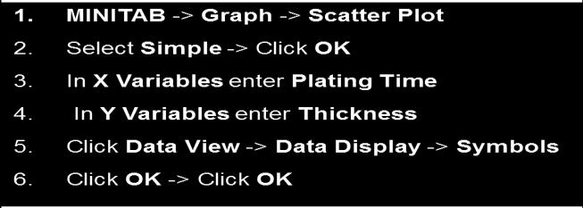
71 Simple Linear Regression and Correlation Analysis 1299 Step I: Plot a Scatter Diagram Simple Linear Regression and Correlation Analysis Step II: Fit a line to the plotted data 1300 Fitted line has a positive slope, suggesting a positive, linear relationship between concentration and thickness Quite a few points fall on the line, suggesting a good relationship between the two variables 71

72 Simple Linear Regression and Correlation Analysis 1301 Step III: Use Least Squares Method to find the best-fit line The best-fit line is found so that the sum of the squared deviations is as small as possible Terminology β 0 and β 1 are also known collectively as coefficients Y is the response or dependent variable X is the independent or predictor variable Simple Linear Regression and Correlation Analysis 1302 Notes The least-squares best-fit line equation is y = β 0 + β 1 x where 0 is the intercept and 1 is the slope of the line The least-squares equations for 0 and 1 are: β 0 = y β 1 x and β 1 = x i x y i y x i x 2 i where i = 1,2,3 n 72

73 Simple Linear Regression and Correlation Analysis 1303 Calculating the coefficients, β 0 and β 1 X Y =99 =82.51 =110 = Note The difference between the predicted value of y and the actual observed value is called residual Residuals are random and should follow the normal distribution Xbar=9 Ybar=7.5 Simple Linear Regression and Correlation Analysis 1304 From table, β 1 = = , β 0 = = 3.0 Substituting these values into our equation, we have y = x This equation is the prediction equation or equation of the regression line Using this equation, one may now predict y for any given value of x. 73

74 Simple Linear Regression and Correlation Analysis 1305 Step IV: Determine the Strength of the relationship between X and Y Note If there is a very strong association between X and Y, then any increase or decrease in X will lead to a corresponding increase or decrease in Y. For example, our regression equation is telling us that plating thickness increases by 0.5 microns for every unit increase in concentration. Simple Linear Regression and Correlation Analysis 1306 A statistical measure of the strength of this association is called correlation coefficient, denoted by r r is a statistic which is a point estimate of the population parameter, ρ r can take on any value between -1 and +1 When r = 1 or r = -1, we say there is perfect correlation when r = 0, there is no correlation See next slide for the calculation of r 74

75 Simple Linear Regression and Correlation Analysis = 110 = = Simple Linear Regression and Correlation Analysis 1308 Using summarised data from table we have ( x x)( y y) r 2 2 ( x x) ( y y) r (110)( ) One can conclude, from the value of r obtained above, that there is good correlation between chemical concentration and plating thickness. 75

76 Simple Linear Regression and Correlation Analysis 1309 Step V: Determine how well our Regression line fits our data One measure of fit is the Coefficient of Determination, denoted by R-Sq. R-Sq is the square of the correlation coefficient, r The value of R-Sq is between 0 and 1 A value near 1 shows a good fit From the previous slide, given that r = 0.82, then R-Sq = (0.82) 2 = 0.67 Simple Linear Regression and Correlation Analysis 1310 This value of R 2 tells us that 67% of the variability in the y data can be explained by the regression model or 67% of the time, we will predict y correctly. Thus one can conclude that the fit of our regression line to the data is better than average. 76

77 Confidence Intervals for Coefficients, βi 1311 They are useful for determining if an independent variable should remain in the equation If coefficient s confidence interval includes a zero value, then corresponding independent variable must be removed from equation Confidence Interval is given in terms of 100(1- α)%, eg 95% Calculation of C.I requires knowledge of estimates of coefficients and standard error (s.e) of coefficients obtained using software such as MINITAB Confidence Intervals for Coefficients, βi 1312 t i, nk 1 2 s. e( ) i i t i, nk 1 2 s. e( ) i 77

78 1313 Confidence Intervals for Coefficients, βi t, nk1 2 Ex. = value obtained from t tables (n = no. of observations, k = no. of independent variables ) Given n = 10, alpha =.05, s.e( 1 ) = and s.e( 2 ) = Find 95% confidence intervals for 1 and 2 y i x x 2 Statistical Decision Making 78

79 Terms and Definitions 1315 Point Estimation A single value obtained from a sample that is used to make a best guess as to what the population parameter is. Eg, a point estimate of the population mean, µ, is the sample average, X. Interval Estimate Interval within which a parameter of interest will lie. Terms and Definitions 1316 Tolerance Interval Interval that contains a proportion of the product which will meet manufacturing limits at a specified confidence level. Confidence Interval Interval within which a population parameter is expected to lie some percentage of the time 79

80 Terms and Definitions Level of Significance, α risk of being wrong 1317 Confidence level 1 α Confidence Limits upper and lower boundaries of the confidence interval Confidence Interval Confidence Interval for Population Parameters 80

81 General Form 1319 General form of the Confidence Interval: Where L U L = Lower limit of interval U = Upper limit θ = Parameter 1-α = confidence coefficient (level of confidence) 1320 Confidence Interval for population Mean (σ Known) X Z / 2 X n Z / 2 n 81

82 Confidence Interval for population Mean (σ Known) 1321 Ex. A manufacturer produces mouldings. It is known that moulding thickness is normally distributed with a standard deviation of σ = 0.6mm. If a random sample of 15 units has an average thickness of mm, what is the 95% confidence interval that contains the true mean thickness? Ans: µ Confidence Interval for Population Mean(σ unknown) 1322 X t s n X t / 2, n1 / 2, n1 s n 82

83 Confidence Interval for Population Mean μ (σ unknown) 1323 If a sample of 16 yields an average of 12 and an sd of 3, estimate the 95% C.I for the population mean (assuming normal distribution) a) µ b) µ c) µ d) µ Confidence Interval for Population Mean μ (σ unknown) When finding a confidence interval for a population mean based on a sample size n: a) Increasing n increases the interval b) Having to use s instead of n decreases the interval c) The larger the interval, the better the estimate of µ d) Increasing n decreases the interval

84 Confidence Interval for Population Variance When it is desired to determine the confidence interval for the true population variance, σ 2, we use the Chi-square Distribution as follows: s 2 ( n 1) 2, s ( n 1) 2 1, 2 Where s = sample variance, n = sample size and the chi-square values are constants obtained from tables 1325 Ex An engineer calculated a sd of 2.36 from a sample of 10 units and wants to determine the 95% confidence interval on the true variance for the population. What is the resulting confidence interval? Ans: σ

85 Point Estimate and Confidence Interval for Population proportion p 0 pˆ 1327 p Z / 2 p(1 n p) p 0 p Z / 2 p(1 n p) Test of Hypothesis 85

86 Test Of Hypothesis 1329 Null Hypothesis (H 0 ) Hypothesis of no difference The hypothesis to be tested Always contains equality Based on the problem statement Test Of Hypothesis 1330 Example If a vendor makes a strong claim that the average throughput from a new process is higher than that of an existing one, then the Null Hypothesis would state that the average throughput from the new process is not different. This is denoted as H 0 : µ new = µ old 86

87 Test Of Hypothesis Alternative Hypothesis (H 1 ) 1331 is a mutually exclusive statement to the null hypothesis is the hypothesis that we would really like to support Test Of Hypothesis 1332 In the case of the vendor s claim earlier on, the alternative hypothesis could state that the average throughput from the new process is different from that of the existing one, denoted as H 1 : µ new µ old 87

88 Test Of Hypothesis Type I Error The risk of rejecting the null hypothesis when it is, in fact, true Also called producer s risk Probability of occurrence = α = level of significance. Type II Error The risk of accepting the null hypothesis when it is false. Also called consumer s risk Probability of occurrence = β Test Of Hypothesis 1334 Power Ability to correctly reject the null hypothesis The complement of risk, ie Power = 1 - The higher the value of power the better The larger the sample size, the higher the power Reduced risk implies reduced power 88

89 Test Of Hypothesis One-Tail or Directional Test Null Hypothesis 1335 Entire risk is on one side H 0 : µ new µ old Alternative Hypothesis H 1 : µ new > µ old 0 µ 0 Risk = Test Of Hypothesis Two-Tail Test Null Hypothesis 1336 risk is on both sides H 0 : µ new = µ old Alternative Hypothesis H 1 : µ new µ old Risk = /2 Risk = /2 89

90 Test Of Hypothesis 1337 Test Statistic A measure of the distance between the sample estimate and its expected value Calculated from relevant sample statistic Test Of Hypothesis 1338 Critical Value A threshold set by the decision rule. Marks the boundary between acceptance and rejection regions Null hypothesis must be rejected if the absolute value of the test statistic is greater than the critical value Obtained from statistical tables 90

91 Hypothesis Testing 1339 Decision Rules Do not reject Null Hypothesis if absolute value of test statistic falls within this region Rejection Region Rejection Region Critical Value Acceptance Region Critical Value Reject Null Hypothesis if value of test statistic falls in the rejection region or if p-value is less than alpha Test Of Hypothesis Test When to Use Test Statistic D.F z-test 1 mean, n > 30, σ known X 0 Z0 / n -- t-test 1 mean, n 30 or σ unknown X n-1 t s / n z-test 2 means, σ known X 1 X 2 z t-test 2 means, σ unknown, but assumed equal χ2 test Sample Variance Vs Known Variance n 1 +n 2-2 n-1 2 F-test 2 Sample Variances s Top: n 1-1 F 1 s 2 2 Bot: n 2-1 Paired t- test t 0 X X 2 ( n 1) s1 ( n2 1) s n n n1 n2 2 means, paired data d n-1 1 n ( n 1) t0 s D s 2 n n

92 Test Of Hypothesis Scenario 1: One-sample z-test A single-cavity mould has been producing insulators with a mean impact strength of 5.16N-m and a standard deviation of 0.25N-m. A sample of 12 specimens taken from a new lot gives an average impact strength of 4.95N-m. Is the mean impact strength of the new lot significantly different from the past performance of the process? Assume risk of 5%. Solution H 0 : μ = 5.16 H1: µ 5.16 Test Statistic: Z X 0 0 / n? 1341 Test Of Hypothesis 1342 Z 0 is outside of acceptance region, thus we reject H 0 and conclude that mean impact strength of the new lot is significantly different 92

93 Test Of Hypothesis 1343 Scenario 2: One-Sample t-test The nominal specification for filling a bottle with a test chemical is 30cc. An engineer takes a sample of 25 units from a stable process. The average obtained from the sample was 28cc with a s.d of 6cc. At a 5% significance level, can we conclude from these results that the process average is less than 30cc? Solution H 0 : µ = 30, H 1 : µ < 30 What is the test statistic? Test Of Hypothesis

94 Test Of Hypothesis Scenario 3: χ2 test, Sample Variance versus a Known value 1345 A customer requires parts to be produced to ± On the basis of this requirement, your Black Belt concludes that the worst possible s.d acceptable is From your capability charts, you determine that the best machine in the shop is only capable of a s.d of computed from a sample of 25 units. Following consultation with other managers, you decided to accept the customer s order. At the 5% significance level, do you think your decision was a good one? Test Of Hypothesis 1346 Solution H 0 : σ = H1: σ > ( n 1) s 2 Test Statistic 2? 2 From chi-square tables, we obtain a critical value of for d.f = 24 and = 0.05 Since the test statistic is less than the critical value, we fail to reject the null hypothesis and conclude that you were right in accepting the order. 94

95 Test Of Hypothesis Scenario 4: Test of Two Sample Variances 1347 We are interested in purchasing a machine from one of two vendors A and B. The variance of vendor A s machine, based on a sample of 25 units is 100, while the variance of vendor B s machine, based on a sample of 10 is 50. Vendor A claims that this sample variance is a statistical fluke and that the true variance of his machine is smaller. If we were to describe a statistical fluke as something that has less than 1 chance in 100 of occurring, should we accept vendor A s claim? Test Of Hypothesis 1348 Solution: H 0 : Var 1 = Var 2 H 1 : Var 1 > Var 2 = 0.01, Var 1 = 100, Var 2 = 50 Test Statistic F = Var 1 /Var 2 =? 95

96 1349 From F tables we obtain a critical value of 4.73 for d.f Num = 24 d.f Denom = 9. As the test statistic is less than the critical value, we fail to reject the null hypothesis and conclude that vendor A s claim could be valid. Hypotheses Tests for 2 means: σ unknown When population s.d is unknown and we wish to test the hypothesis H 0 : μ 1 = μ 2, assuming σ 1 = σ 2 and σ i unknown, then we use the t distribution 1350 Test Statistic is thus given as follows t 0 2 ( n 1) s1 ( n2 1) s n n 2 1 X 2 1 X n 1 1 n 2 96

97 Ex Two types of plastic are used in a component. The breaking strength is important. It is known that s 1 = s 2 =1.0 psi. From random samples of sizes n 1 =10 n 2 =12 we obtain X 1 = 162.5, X 2 = Based on this information we would like to test the claim that breaking strengths for the two types of plastic are not different, using a level of significance of 0.05 Test Of Hypothesis Paired t-test The data below was obtained by two inspectors measuring the same set of samples. Is there a significant difference between the two inspectors measurements? Assume an alpha risk of 5%. Inspector 1 Inspector 2 Diff(d) d-bar = 1 s D =

98 Test Of Hypothesis 1353 Paired t-test H 0 : µ 1 = µ 2 H 1 : µ 1 µ 2 (Paired t-test is always two-tailed) Test Statistic d t0? sd n Test Of Hypothesis 1354 From t tables and for = 0.025, d.f = 4, we obtain a critical value of As the test statistic is less than the critical value, we fail to reject the null hypothesis and conclude that there is no significant difference between inspectors measurements. 98

99 Test Of Hypothesis 1355 Chi-Square Contingency Tables The table on the next slide is a summary of complaints logged by a mobile operator s call centre, in which customer complaints are classified by geographical region. Is there a relationship between complaint category and geographical region? Assume a 5% significance level. H 0 : There is no relationship H 1 : There is a relationship Test Of Hypothesis 1356 Complaint Category Region Poor Incorrect Poor User Total Connectivity Billing Experience Ulster Leinster Total

100 Test Of Hypothesis Calculate Test Statistic 1357 ( E i O E 2 2 i) where E i = expected frequency and O i = observed frequency of each type of complaints. Ei = [(Row Total) X (Column Total)]/(Grand Total) i Test Of Hypothesis 1358 Region Poor Connectivity Complaint Category Incorrect Billing Poor User Experience Total Ulster 30(31.76) 40(42.35) 20( ) 90 Leinster 30( ) 40( ) 10( ) 80 Total χ 2 = (1.76) 2 /(31.76) + (2.35) 2 /(42.35) + (-4.12) 2 / (-1.76) 2 / (-2.35) 2 / (4.12) 2 /14.12 = =

101 Test Of Hypothesis Thus chi-square test statistic, χ 2 = 2.76 We now need to reference chi-square tables for the critical value, given that = 0.05, and d.f = (rows 1) X (columns 1) = 2 This gives a critical value of As the test statistic is less than the critical value, we cannot reject the null hypothesis. We thus conclude that there is not enough evidence to suggest a relationship between region and complaint category Goodness-Of-Fit Tests Used to determine if a given set of data follows a particular distribution If o1..,ok and np1..,npk are the observed and expected frequencies for the k possible outcomes of an experiment, then for a large n, the distribution of the quantity k ( o1 n p1 ) i1 n p 1 2 is approximately that of a chi-square random variable with (k-1) df. This is the test statistic for a goodness-of-fit test!

102 Methodology 1. State the null and alternative hypotheses H 0 : Data follows a specified distribution H 1 : Data does not follow the distribution Compute expected value, e i where ei = np i ( 3. Calculate Test Statistic, 2 oi 0 e 4. Fail to reject, or reject null hypothesis i e i ) 2 Goodness-Of-Fit Tests Reject H0 if: 0, k p1 where: k = no. of categories p = no of parameters to be estimated from the data α = level of significance Distribution Parameters to estimate p Weibull 3 3 Normal 2 2 Poisson 1 1 Binomial 1 1 Uniform

103 Ex tosses of a die yielded the following results. Do these results follow the uniform distribution? No. Obs. Freq (O i ) Exp. Freq(E i ) (O i -E i ) 2 /E i E i = np i = (1/6) X 48 = 8 Analysis Of Variance (ANOVA) 103

104 One-way Analysis Of Variance (ANOVA) 1365 A statistical technique used to determine if differences exist between the means of three or more populations Used to answer the question: What is the effect of one categorical variable or factor on the mean response? Tests the hypothesis H 0 : µ 1 = µ 2 = = µ n Vs H 1 : µ 1 µ 2 Partitions total variation into variation between treatments and variation within treatments Variation is presented in tabular form called ANOVA table One-way Analysis Of Variance (ANOVA) 1366 Source Of Variation Sum Of Squares (SS) Degrees of Freedom (DF) Mean Squares (MS) Between Treatments SST DF T = (t-1) MS T = Within Treatments(Error) SSE DF Error = (N-1) (t-1) = N-t SS T /DF T MS Error = SS Error DF Error F Ratio MS T MS Error Total SS Total DF Total = N-1 N = number of measurements, t = number of treatments 104

105 One-way Analysis Of Variance (ANOVA) 1367 One-way Analysis Of Variance (ANOVA) 1368 Then CM GM x N x 2 N SST SS Total SSE n t x t GM x 2 2 CM SS Total SST 105

106 ANOVA Example 1369 We have three machines producing a particular component. We wish to compare the average of a certain dimension. The table on the next slide shows coded measurements obtained from these machines. Is there a real difference in the mean settings of the machines? ANOVA Example 1370 Machine Data x n x 2 A B C Totals H 0 : µ 1 = µ 2 = µ 3, H 1 : At least one machine is different 106

107 1371 ANOVA Example 1372 When compared to a critical value, we would reject the null hypothesis if F statistic is greater than the critical value and support the alternative hypothesis that at least one group mean is different Use of p-value. p-value states the probability of obtaining the observed F statistic if the population means are equal A small p-value suggests that the null hypothesis is false 107

108 One-way Analysis Of Variance (ANOVA) 1373 Q1. Consider the SS and MS columns of an analysis of variance table for a single factor design. The appropriate ratio for testing the null hypothesis of no treatment effect is 1. SS treatments divided by SS residual 2. MS treatment divided by MS residual 3. SS treatment divided by MS residual 4. MS treatment divided by SS residual 1374 Q2. The test used for testing significance in an analysis of variance table is the 1. Z test 2. t test 3. F test 4. Chi-square test 108

109 One-way Analysis Of Variance (ANOVA) Q3. A designed experiment has been conducted at three levels (A, B and C) yielding the following coded data A B C As a major step in the analysis, one would calculate the degrees of freedom for the error sum of squares to be:

110 One-way Analysis Of Variance (ANOVA) Q4. One-way analysis of variance is most similar in its objectives to 1. A test of population mean 2. A test for equality of two sample proportions 3. A test for equality of two population means 4. A chi-square test for independence

111 1379 Statistical Process Control 111

112 Definitions 1381 SPC is the use of statistical techniques to measure, monitor, control and hence reduce undesirable variability in processes and products, thereby improving overall quality and productivity. SPC assumes that variation exists in every process This variation is categorised as chance or common cause variation and assignable or special cause variation. Objectives and Benefits 1382 Objectives To use data gathered from the process as a tool for developing a strategy for process improvement and sustenance of the state-of-control Benefits Reduced manufacturing costs due to reduction in waste and scrap 112

113 Objectives and Benefits 1383 Improved customer satisfaction by consistently manufacturing to agreed requirements or specifications Improved competitiveness through over-all improvement in quality, reliability, delivery and price Concepts Variability deviation, inconsistency or lack of repeatability exhibited by a process, the magnitude of which could lead to the production of non-conforming items Two Sources Of Variability Common Cause Inherent in the process Small in magnitude Occur at random and follow the normal distribution 1384 Process with only common cause variation is said to be in a state of statistical control. 113

114 Concepts Assignable (Special) Cause Variation above and beyond common cause variation, arising from factors that are not always present in the process Externally induced Characteristically large in magnitude Not random - tend to follow a pattern or trend Process could be out of control if assignable causes are at play 1385 Concepts Rational Sub-grouping The process of selecting a subgroup based on some logical grouping criteria or statistical consideration Two approaches to rational sub-grouping 1. Take samples in order of manufacturing sequence Used for control charts intended to monitor shift in the process setting 1386 Minimises effect of within sample variation, but maximises between sample variation 114

115 Concepts Take a random sample from the batch of units produced since the last sample was taken Used when chart is intended for making acceptance decision with regard to the process output since the last sample was taken Control Charts A control chart is a form of time series plot that has the added features of a mean line and control limits. It is a tool that is used to dynamically monitor process performance over time from the view-point of detecting a state of out-of-control. Two types Variables Charts Used for controlling measurable characteristics, e.g. temperature, weight, diameter, voltage, etc

116 Control Charts 1389 These charts use sample means to monitor process centering and either sample range or standard deviation to monitor variation Attributes charts Are based on data that follow a discrete distribution Work to process capability Control Charts Charts generally have two sets of limits 1390 Warning Limits (Not used in the USA) Also known as 2-sigma limits Probability of a point plotting outside of these limits is 1 in 40 or Thus when this happens, we must take it as a warning sign. As the chance of 2 consecutive points plotting outside the limits is 1 in 1600, when this happens, we must take action 116

117 Control Charts 1391 Action Limits (Control Limits in the USA) Also known as 3-sigma limits When process is in control, probability of a point plotting outside of action limits is approx 1 in Thus when this happens, the process is said to be out of control, so action must be taken to bring it back into control All limits are located symmetrically about the mean or aim of the process Statistical Process Control 117

118 Control Charts for Continuous Data In most cases, two charts are created for each set of continuous data Charts showing individual data points or subgroup averages These charts show changes in the average value of the process They represent a visualisation of the longer-term variation of the process Control Charts for Continuous Data Charts showing the range or moving range of subgroup data These charts reflect short-term variation They answer the question Is the variation within subgroups consistent? 118

119 Individuals and Moving Range (ImR) Charts Individual measurements are plotted instead of averages. Measured data is not collected in subgroups Calculating Control Limits UCL LCL X E 2 ( MR) CL X X E 2 ( MR) 1395 ImR Charts

120 ImR Charts 1397 Creating an ImR Chart 1. Determine sampling plan. 2. Take one unit at each time or at each production interval. 3. Calculate moving ranges for by subtracting each measurement from the previous one. 4. Plot individual measurement on one chart and moving ranges on another. Continued ImR Charts 1398 Creating an ImR Chart 5. After 20 or more data points, calculate the limits for the range chart. 6. If range chart is in control, calculate limits for the individuals chart. 120

121 ImR Charts 1399 Stats > Control Charts > Var Charts for Ind Weights of Bags ImR Charts 1400 Advantages of ImR Charts Useful when large samples are not readily obtainable or too expensive to analyse Easy to construct and apply Useful in the early stages of process set-up or development Useful where within batch variation is small compared to between batch variation 121

122 ImR Charts 1401 Disadvantages of ImR Charts Insensitivity to substantial changes in process averages Average and Range Charts

123 Average and Range Charts Limits for Average Chart UCL X A 2 R LCL X A 2 R CL X 1403 Limits for Range Chart UCL D 4 R LCL D 3 R A 2, D 3 and D 4 are control chart factors to be obtained from tables Minitab Xbar-R Stats>Control Charts>Charts for Subgroups Average and Range Charts

124 Average and Range Charts 1405 Average and Range Charts Ex. Construct Average and Range Charts from the following data

125 Average and Standard Deviation Charts 1407 Used when subgroup sizes are large ( 10) and use of standard deviation is preferred to range. (SD gives a better measure of dispersion than range). Have the disadvantage of being more complex than average and range charts Average and Standard Deviation Charts

126 Average and Standard Deviation Charts Calculate Control Limits for the Average Chart 1409 UCL X A 3 s LCL X A 3 s CL X Calculate Control Limits for SD Chart UCL B s LCL B 4 3 s Average and Standard Deviation Charts Ex. Construct Limits for Average and SD charts using the following data

127 Control Charts for Attributes Creating Charts for Attribute Data 1. Determine an appropriate sampling plan 2. Take samples at specified intervals of time 3. Calculate the relevant metric p, np, c or u 4. Calculate the appropriate centre line 5. Plot the data 6. After 20 or more data points, calculate the limits 7. If the chart is not in control, take appropriate action

128 Proportion Defective Chart (p-chart ) 1413 p-chart

129 p-chart 1415 Calculate Control Limits UCL p 3s LCL p3s CL p Note that if LCL is negative, then it must be set to zero, as proportion defective can never be less than zero p-chart 1416 Ex. Compute control limits for a proportion defective chart using the data below. No. Sample Rejects Size

130 Number Defective Chart (np-chart) 1417 Similar to p-chart, but controls actual number of products not conforming to specifications Subgroup or sample size must be constant Control Limits UCL n p 3 n p1 p LCL n p3 n p1 p CL n p np-chart days of inspection of typed documents yielded the errors shown in the table below. Use this data to construct a number defective chart. Day Sample Errors

131 Number Of Defects Chart (c-chart) The c-chart is used for monitoring a count of defects on a unit of product such as imperfections on a painted part Data for this chart follows the Poisson distribution It is suitable when subgroup sizes are constant c-chart 1420 Calculating Control Limits is a two-step process: 1. Estimate average number of defects c c k where c = defects per subgroup and k = number of subgroups inspected continued 131

132 c-chart Calculate the limits UCL c 3 c LCL c3 c CL c where CL is the centre line of chart c-chart 1422 Example Inspection of 20 painted coach doors for imperfections yielded the following results. Use the data to construct a c-chart to control the process

133 Number Of Defects per Unit Chart (u-chart) The u-chart monitors the average number of nonconformities per inspection unit. It is suitable when subgroup size can vary. Data follows Poisson distribution u-chart 1424 Calculating Control Limits is a two-step process: 1. Estimate average number of non-conformities. c u i n i where c i = non-conformities in subgroup i; and n i = size of subgroup i continued 133

134 u-chart Calculate the Limits n UCL u3 LCL n i k u u n 3 u n where k = number of subgroups u-chart 1426 The following data shows the number of defects on turbine blades. Calculate the control limits for an appropriate chart. No Sample Size Defects

135 Chart Interpretation Use the following rules to determine if a chart is in control or not One point plotting outside of control limits is evidence of an out-of-control condition Seven points or more plotting above or below the centre line constitutes a run, indicating that the process is not stable or is about to change its aim 1427 Chart Interpretation 1428 Six consecutive points in an upward or downward direction constitutes a trend, indicating that the process is drifting and thus is not in statistical control. Timely corrective action must be taken in each of the above situations, or else out-of-tolerance work will be produced 135

136 Pre-Control Used to monitor the capability of a process to meet specification limits 1429 Uses the normal distribution to detect changes in process mean and dispersion Outer limits are product specification limits, ie USL and LSL respectively Pre-Control 1430 Outer limits are assumed to correspond to μ ± 3σ Process target is assumed to coincide with μ Pre-Control Limits Upper PCL = (Target + USL)/2 Lower PCL = (Target + LSL)/2 continued 136

137 Pre-Control 1431 Process Verification Select and measure 5 consecutive units If all 5 units plot within PC limits, continue production If one point plots outside PC limits, take additional samples and repeat If 2 consecutive points plot outside PC limits, reset the process and start again Pre-Control On-going Operation 1432 Take 2 consecutive samples periodically 1. Reset the process if the first unit plots outside the specification limits (SL) 2. If the first item plots outside the PC limits, but within SL, check the next item 3. If the second item plots outside the PC limit on the same side as the first, reset the process 137

138 Pre-Control Continue production if second unit plots within PC limits 5. Investigate and eliminate cause if one item plots outside PC limit on one side of target and second item plots outside limit on the other side of the target This is indicative of an increase in process variability Pre-Control Advantages of Pre-Control 1434 Ease of implementation and use Requires very few computations Very useful when process has no history and it is essential to quickly determine its capability 138

139 Pre-Control 1435 Disadvantages Unlike control charts, it does not lend itself to trend or run analysis Not sensitive enough to detect moderate to large changes sample size too small Does not provide enough information about variability Not suitable for use with process with capability index less than 1. Result will be unnecessary frequent stop/start of the process Short-Run SPC

140 Short-Run SPC 1437 Construction During each visit to the process, take a sample, size n, and measure each item. Repeat the above procedure up to k visits (typically 20) 1438 How to Calculate Limits 1. Given a nominal value (T i ) for each sample, determine deviation of each item from nominal value such that d ij = x ij T i where d ij = deviation of item j, sample i; and x ij = item j in sample i continued 140

141 Determine the average deviation within each sample d i n d ij 1440 Determine range, R i for each sample Determine Mean Range and grand mean of the deviations R d Ri n k d i 141

142 1441 Calculate Limits for the Deviations Chart CL d UCL d A 2 R LCL d A 2 R Where CL = Centre line, A2 is constant from tables, UCL and LCL are upper and lower limits 1442 Calculate Limits for the Range Chart CL R UCL LCL D D 4 3 R R D 3 and D 4 are constants from tables 142

143 1443 Design of Experiments 143

144 Design Of Experiment 1445 What is DOE A test or series of tests in which deliberate changes are made to controllable variables of a process in order to effect a corresponding change in a response variable Application Process Characterisation Process Optimisation Product Design Terms and Definitions 1446 Independent Variables Controllable inputs which can be manipulated to bring about a corresponding change in the response variable Dependent Variable The response variable, or that variable which changes its state as a result of a change in one or more inputs 144

145 Terms and Definitions 1447 Factor A variable or attribute that can effect a change in the output or result of an experiment; eg temperature, concentration of a chemical bath, etc Levels Settings or values of the factors at which observations of the dependent variable are made Terms and Definitions 1448 Replication Replicates are the number of observations for a specific factor level Treatment A unique combination of factors in an experiment For a general factorial design, it represents the levels of the factor. 145

146 Terms and Definitions 1449 Model A mathematical representation of the relationship between a response variable and independent variables Eg one-way analysis of variance model is yij Where yij = response; μ = over-all mean; i ij τi = effect of i th factor; εij = error Terms and Definitions 1450 Error Observed variability when a treatment is replicated Fixed-Effects Model Factor levels are specifically chosen by the experimenter Conclusions are specific to the chosen levels and cannot be extended to other levels 146

147 Terms and Definitions 1451 Random Effects Model Also called Components-of-variance model Factor levels are a random sample from a large population of levels Planning an Experiment 1452 Define objective Choose factors to be varied and specific levels at which measurements are to be taken Select response variable continued 147

148 Planning an Experiment 1453 Choose experimental design methodology Sample size, blocking, randomisation, etc Perform the experiment Analyse the data Draw conclusions and make recommendations Planning an Experiment Other Considerations 1454 Power Sample size Run Order Efficiency Randomisation Confounding Interaction 148

149 Measurements Randomised One-factor Experiment General Model yij i j ij 1455 Where y ij =response, µ = overall mean, τ i = effect of treatment i, β j = effect of treatment j and ε ij = error Objective To compare observed treatment means If means are close together, then differences are not significant (may be attributable to residual variation) Thus H0: τ 1 = τ 2 =. = τ c H1: One or more treatments is different Randomised One-factor Experiment The effect of temperature on the yield of a particular process was investigated at three settings as shown below. Temperature Settings Means Design an experiment that will answer the questions on the following slide(s)

150 Randomised One-factor Experiment How many factors are being investigated in this experiment? 2. How many levels are being considered 3. How many replicates per level? 4. What is the response variable 5. What is signal-to-noise ratio? continued Randomised One-factor Experiment 6. Is our data normal? 7. From ANOVA table, validate SS,DF, MS and F 8. The null hypothesis (no difference between treatments) should be rejected at the α=0.05 level. True or false? 9. What is R-Squared? 10. What is CV%

151 Analysis of Randomised One-factor Experiment 1459 Source SS df MS F p-value Treatment Pure Error Total Std. Dev R-Squared Mean Adj R-Squared C.V. % 5.76 Randomised Block Design 1460 Blocking Provides a homogeneous environment for experimentation Blocking minimises or reduces bias which could be caused by some uncontrolled variable We might, for example, block the effect of Days on a response variable 151

152 Randomised Block Design 1461 If we have to spread the testing over a number of days, then it s quite possible for unforeseen differences to arise during certain days of experimentation. We must therefore plan to provide a homogeneous environment for testing so as to ensure unbiased results regardless of the day of the test. Randomised Block Design 1462 We can, for instance randomly select 5 runs to be performed each day, such that run 4, 15, 2, 10 and 35 would be performed on Monday and another combination of 5 on Tuesday, etc. This technique will help to nullify the impact of dayrelated changes and is called Randomised Block Design. 152

153 ANOVA Table (Randomised Block Design) 1463 Source of Variation SS DF MS F 0 Treatments (t) SST t-1 MST=SST/ t -1 MST/MSE Blocks (b) SSB b-1 MSB = SSB/b-1 Error (within) SSE (t-1)(b-1) MSE = SSE/(t-1)(b-1) Total Variation SS T n-1 ANOVA Table (Randomised Block Design) Where SST = [(TreatmentTotal) 2 /n Treatment ] - CM SSB = [(BlockTotal) 2 /n Block ] - CM TotalSS = x 2 - CM SSE = TotalSS SST SSB CM = ( x) 2 /N

154 Factorial Experiments 1465 Used for investigating more than one factor Combinations of levels of factors are investigated Two Types of Factorial Designs: 1. Full factorial with k factors each at 2 levels Several factors, each at several levels Factorial Experiments 2. Fractional Factorial Sub-set of runs required for full factorial General Model of 2-Factor Factorial y ijk ( ) for i = 1,2 a; j = 1,2, b; k=1,2,n Where μ= overall mean effect τ i = effect of level i in factor A i βj = effect of level j in factor B j ij ijk 1466 (τβ) = effect of interaction between A and B 154

155 Factorial Experiments General Factorial Design with two factors (Material & Instructor). Material (A) Instructor(B) ANOVA Table (2-Factor Factorial Exp) Source of Variation SS DF MS F Factor A SS A a-1 MS A =SS A / a-1 MS A /MS e Factor B SS B b-1 MS B = SS B /b-1 MS B /MS e Interaction SS AB (a-1)(b-1) MS AB = SS AB /(a-1)(b-1) MS AB /MS e Error (within) SS e n - ab MS e = SS e /(n-ab) Total Variation SS T n-1 155

156 ANOVA Table (2-Factor Factorial Exp) Note: 1469 A and B in ANOVA table above are row and column effects respectively Test H 0 that there is no difference between rows, between columns and no interaction between A and B factors Use corresponding F 0 ratio as test statistic For given alpha, use corresponding df to determine critical value from F-table ANOVA Equations (2-Factor Factorial Exp) 1470 TotalSS = ( x 2 CM) ColSq = ( Col) 2 /n col, RowSq = ( Row) 2 /n row ColSS = ( ColSq CM) RowSS = ( RowSq CM) SSE = TotalSS ColSS - RowSS Where CM = ( X) 2 /N Analyse the design on slide

157 Two-Way Analysis of Variance 1471 Source SS DF MS F p Instructor Material Instructor *Material Error Total Main Effects Plot

158 Interaction Plot 1473 Latin Square Design Used when one primary factor is being investigated and the results may be affected by two other factors The following criteria must be met: Each treatment must occur only once in each row and each column The number of treatments must equal the number of rows and number of columns There should be no interaction between row and column factors

159 ANOVA Table for Latin Square Design 1475 Source SS df MS F Rows (r) SSr dfr=r-1 SSr/dfr MSr/MSe Cols (c) SSc dfc=c-1 SSc/dfc MSc/Me Treatment (t) SSt dft =t-1 SSt/dft MSt/MSe Residual SSe df T - dft- dfc-dfr SSe/dfe Total SST df T =rc-1 Latin Square Example 1476 The table on the next slide shows a 4x4 Latin Sq. design of an experiment to investigate the effects of 4 additives, A,B,C and D on fuel consumption of 4 cars which are driven by 4 drivers. The objective is to determine if there is a significant difference between cars, between additives, and between drivers 159

160 Latin Square Example 1477 CAR D r i v e r I D(20) A(21) B(26) C(25) II A(20) D(23) C(26) B(27) III C(16) B(15) D(13) A(16) IV B(20) C(17) A(15) D(20)

161 Reliability and Risk Management Terms & Definitions 1480 Reliability (R(t)) Probability that a component or system will perform its required function under stated conditions and for a specified period of time Note Reliability is a probability it cannot be stated with complete certainty! When stating reliability, one must specify function, time and operating environment 161

162 Terms & Definitions Failure The termination of the ability of an item to perform a required function (BS 4778) Note Failure is the inverse of reliability Failure Rate (λ) The number of failures per unit time. The ratio of the total number of failures in a sample to the cumulative observed time on that sample (Observed Failure Rate) 1481 Terms & Definitions 1482 Hazard Function Also called Instantaneous Failure Rate, this is the failure rate at a particular instant in time. Denoted by z(t) and calculated by: (No. time t per unit time)/(no. surviving at that time) 162

163 Terms & Definitions 1483 Mean Time Between Failures (MTBF ) The mean value of the length of time between consecutive failures computed as the ratio of cumulative observed time to the number of failures under stated conditions (BS 4778) Also a measure of reliability of a repairable unit or system Terms & Definitions 1484 Mean Time To Failure (MTTF) For a stated period in the life of an item, the ratio of the failures in a sample to the cumulative observed time on that sample MTTF is a measure of reliability of non-repairable items MTBF and MTTF are equivalent quantities 163

164 Terms & Definitions 1485 Mean Time To Repair (MTTR) The value of the mean time required to restore a failed unit or system to its full functional state Also defined as the total corrective maintenance time divided by the total number of corrective maintenance actions during a given period of time (MIL-STD-721B) Only applicable during useful life Terms & Definitions Maintainability Ability of an item, under stated conditions of use, to be retained in, or restored to, a state in which it can perform its required function(s) (Part BS4778 definition). Corrective Maintenance The actions performed, as a result of failure, to restore an item to a specified condition (MIL-STD-721B)

165 Terms & Definitions Preventive Maintenance The actions performed in an attempt to retain an item in a specified condition by providing systematic inspection, detection and prevention of incipient failure (MIL-STD- 721B) Observed B-percentile Life The length of observed time at which a stated proportion (B%) of a sample of items has failed (BS 4778) 1487 Terms & Definitions 1488 Availability Ability of an item (under combined aspects of reliability, maintainability and maintenance support) to perform its required function at a stated instant of time or over a stated period of time (BS 4778) 165

166 Terms & Definitions 1489 Redundancy The existence of more than one means for accomplishing a given function. Each means of accomplishing the function need not necessarily be identical (MIL-STD-721B) Terms & Definitions 1490 Active Redundancy The redundancy wherein all redundant items are operating simultaneously rather than being switched on when needed (MIL-STD-721B) 166

167 Terms & Definitions 1491 Standby Redundancy The redundancy wherein the alternative means of performing the function is inoperative until needed and is switched on upon failure of the primary means of performing the function (MIL-STD-721B) Reliability Life Characteristics Concepts 167

168 Bathtub Curve A plot of failure rate vs time 1493 Used to model failure patterns during product life cycle The curve can be divided into three main zones, namely infant mortality (or early failure), Useful life and wearout zones respectively Bathtub Curve

169 Bathtub Curve 1495 Early Failure Period Characterised by decreasing failure rate (DFR) Pattern of failure is due to inclusion of weaker than specified components Bathtub Curve 1496 Constant Failure Period Characterised by random and usually fewer failures per unit time (CFR). Failure pattern is constant, failures being as a result of externally induced factors 169

170 Bathtub Curve 1497 Wear-Out Failure Period Characterised by increasing failure rate (IFR) This zone marks the period in which good items begin to fail due to wear and tear. Probability Distributions and Zones of the Bathtub Curve 1498 Copyright 2006 Global Business Institute. All rights reserved. 170

171 Normal Distribution and Wear-Out Zone 1499 In the wear-out zone failure occurs due to natural wear and tear. Thus assuming proper preventive maintenance, it is reasonable to expect failure of components to be predictable and to follow the normal distribution. We use the standard normal variable, Z, as follows: z t 1 Normal Distribution and Wear-Out Zone Where 1500 t 1 = the specified time μ = mean wear-out time σ = standard deviation The value of z is the number of standard deviations from the mean The area of the normal curve to the right of z is the reliability value of interest 171

172 Normal Distribution and Wear-Out Zone 1501 Notes 1.When the normal distribution is used, 50% of the population will have failed when the observed B-life is equal to the mean wear-out time 2.Beginning of wear-out zone is often assumed to be between 3.5σ to 4.5σ to the left of the mean Normal Distribution and Wear-Out Zone 1502 Exercise The life of a bulb is normally distributed, with mean 1200h and standard deviation of 200h. What is the probability of the bulb lasting a. At least 800h (0.9773) b. At least 1400h (0.1587) 172

173 Exponential Distribution and Useful Life Zone Failure in this zone is characterised by random and usually fewer failures per unit time and cause of failure is usually due to external factors. It is possible to predict a failure in this zone within a certain time interval, but not a specific failure at a specific time. The exponential distribution is the most suitable for modelling data obtained from this period Exponential Distribution and Useful Life Zone The exponential distribution describes the situation wherein the instantaneous failure rate is constant Its pdf is given by: t f ( t) 1 e where θ = mean life, also called MTBF (for repairable items) and t is the independent variable (or mission time)

174 Exponential Distribution and Useful Life Zone The probability of no failure before time t is obtained by integrating the pdf equation and subtracting from R(t) is the reliability function or probability of survival up to time t and can be used to predict survival or its inverse, failure. Use of the Weibull Distribution 1506 The Weibull has many applications in Reliability work As the value of shape parameter β changes, the Weibull distribution approximates other distributions as follows: When β = 1, distribution approximates exponential When β > 1, distribution approaches normal When β< 1, distribution approaches lognormal, depending on sample size 174

175 Use of the Weibull Distribution Shape parameter of the distribution also reflects underlying failure rate pattern as shown in the table. Value of β Failure Rate β<1 Decreasing β=1 Constant Β>1 Increasing 1507 Reliability and Failure Analysis 1. time t 1508 R(t) = (No. surviving at time start (t=0)) 2. Instantaneous Failure Rate z(t) = (No. Failing per unit time t)/(no. time t) 3. MTBF (or MTTF) θ = (Cumulative Observed time)/(total No. Of failures) = 1/(Failure Rate) 175

176 Reliability and Failure Analysis Exercise During a test of a system consisting of 20 components the failure pattern shown in the table was observed. The test was terminated after 1000 hrs. Assuming replacement of failed units, find an estimate of the failure rate Ans per hr. Unit Hours survived Reliability and Failure Analysis Failure pdf f(t) = R(t) x z(t) 5. Hazard function z(t) = h(t) = f(t)/r(t) When a constant failure rate is assumed, then z(t) = λ 176

177 Reliability and Failure Analysis From (3) and (5) above, we have MTBF = MTTF = θ = 1/λ and λ = 1/ θ 7. We have already shown that R( t) e t Thus R( t) e t Reliability and Failure Analysis 1512 Ex. 1 A component has an MTBF of 6000h. What is the probability that it will fail after 7000h? Ans Ex. 2 A unit has a constant failure rate. The variance of time to failure is 100. What is the mean time to failure? Ans. 10hr 177

178 Reliability and Failure Analysis time t, given survival up to time t 1 R( t t 1 ) R( t t1) R( t ) 1 9. Availability Availability MTBF ( MTBF MTTR) Reliability and Failure Analysis 10. System Reliability at time t, assuming Series Configuration of n components R sys ( t) e... ) t where λ sys = system (constant) failure rate sys t e ( 1 2 n e nt 1514 = λ 1 + λ λ n 11. Mean Time to Repair MTTR e

179 Reliability and Failure Analysis Ex Three sub-assemblies are connected in series to form a main system. Each sub-assembly is known to exhibit a constant failure rate of 0.003, and respectively. Compute System MTTF System Reliability after 1000 hrs of operation

180 Systems Design for Reliability Reliability Modelling Series Systems 1518 System comprises of a number of sub-systems in series There is only one path for the signal Failure of any one sub-system will result in entire system failure 180

181 1519 Series Systems Assume constant failure rate for each sub-system: λ 1, λ 2, λ 2 Thus system failure rate, λ s is given by 1520 λ s = λ 1 + λ λ n System Reliability R s = R 1 x R 2 x. x R n R s e OR ( n ) t 181

182 Series Systems Exercise 1521 Three sub-assemblies are connected in series to form a main system. Each sub-assembly is known to exhibit a constant failure rate of 0.003, and respectively. Compute System MTTF System Reliability after 1000 hrs of operation Parallel Systems (Active Redundancy) There are two or more sub-systems in operation at any one time 1522 System will function satisfactorily if any one sub-system is operational 182

183 Parallel Systems (Active Redundancy) 1523 Failure of any sub-system is independent of other subsystems Failure of one sub-system does not affect reliability of other sub-systems no load increase results Failure of one sub-system does not diminish the functionality of the main system Parallel Systems (Active Redundancy) System reliability is P(A or B) = P(A+B) Since failure of sub-systems is independent, then P(System Failure) = [1-R 1 ]x[1- R 2 ] Thus R s = System Reliability = 1 - System Failure = 1 [(1-R 1 )(1-R 2 ) (1-R n )] for n sub-systems

184 Parallel Systems (Active Redundancy) 1525 Example A system comprising of three sub-assemblies is configured for active redundancy. Reliability of each sub-assembly is 0.95, 0.98 and 0.93 respectively. What is the reliability of the system? Ans Rs = 1 [(1-0.95)(1-0.98)(1-0.93)] = 1 [0.05 x 0.02 x 0.07] = m-out-of-n Parallel Systems 1526 A form of redundancy whereby only m of n sub-systems are required to function in order for the system to function successfully Also referred to as m of n or m/n system, where m < n. Reliabilities of all n units are equal 184

185 m-out-of-n Parallel Systems 1527 The mission is successful if m out of n sub-systems or components function, otherwise mission fails System reliability is the (cumulative) binomial reliability function Thus R s ( t) n i ni R (1 R) i i m-out-of-n Parallel Systems 1528 Exercise A missile system comprises of six identical sub-systems in active redundancy. The system will be successful if at least four of the sub-systems function successfully. Given that the reliability of each sub-system is 0.95, what is the probability that the system will succeed? 185

186 m-out-of-n Parallel Systems 1529 Ans R(t) = P(4) + P(5) + P(6) P(4) = [6!/(6-4)! (4!)] x [0.95] 4 x [.05] 2 P(5) = [6!/(6-5)! (5!)] x [0.95] 5 x [.05] 1 P(6) = [6!/(6-6)! (6!)] x [0.95] 6 x [.05] 0 R(t) = = Standby Redundancy Achieved when a redundant unit does not operate until switched on, upon failure of the primary unit 1530 Switching/sensing device has one-shot reliability. (Oneshot items only operate when called upon, thus resulting in instant success or failure) 186

187 Standby Redundancy 1531 Key Assumptions Standby unit is identical to primary unit Primary and standby units both have equal, constant failure rates Sensing and switching devices have reliability of 1 Standby Redundancy 1532 Under above assumptions, system reliability is represented by: R ( t) e s t t( e t ) 187

188 Standby Redundancy 1533 Exercise A servo system is configured as a primary unit which must operate for 130 consecutive hours. An identical unit, having an equal constant failure rate of /h is set up as a stand-by unit. What is the probability that the system will stay operational for the full 130-hour mission? Standby Redundancy 1534 Ans R s (130) = e -(0.0020x130) + (0.002x130)[e -(0.002x130) ] = x =

189 Series-Parallel System 1535 Combination of both series and parallel sub-systems Series-Parallel System 1536 To obtain system reliability, combined sub-system and system reliabilities must be converted to either series or parallel. Appropriate formula may then be applied to resulting system configuration 189