Electromagnetic Wave Propagation Lecture 2: Time harmonic dependence, constitutive relations

Transcription

1 Electromagnetic Wave Propagation Lecture 2: Time harmonic dependence, constitutive relations Daniel Sjöberg Department of Electrical and Information Technology September 2015

2 Outline 1 Harmonic time dependence 2 Constitutive relations, time domain 3 Constitutive relations, frequency domain 4 Examples of material models 5 Bounds on metamaterials 6 Conclusions 2 / 53

3 Outline 1 Harmonic time dependence 2 Constitutive relations, time domain 3 Constitutive relations, frequency domain 4 Examples of material models 5 Bounds on metamaterials 6 Conclusions 3 / 53

4 Scope The theory given in this lecture (and the entire course) is applicable to the whole electromagnetic spectrum. However, different processes are dominant in different bands, making the material models different. Today, you learn what restrictions are imposed by the requirements 1. Linearity 2. Causality 3. Time translational invariance 4. Passivity 4 / 53

5 Electromagnetic spectrum, c 0 = fλ m/s Band Frequency Wavelength ELF Extremely Low Frequency Hz 1 10 Mm VF Voice Frequency Hz km VLF Very Low Frequency 3 30 khz km LF Low Frequency khz 1 10 km MF Medium Frequency khz m HF High Frequency 3 30 MHz m VHF Very High Frequency MHz 1 10 m UHF Ultra High Frequency MHz cm SHF Super High Frequency 3 30 GHz 1 10 cm EHF Extremely High Frequency GHz 1 10 mm Submillimeter GHz µm Infrared THz µm Visible THz nm Ultraviolet 750 THz 30 PHz nm X-ray 30 PHz 3 EHz 10 nm 100 pm γ-ray >3 EHz <100 pm 5 / 53

6 Three ways of introducing time harmonic fields Fourier transform (finite energy fields, ω = 2πf) E(r, ω) = E(r, t) = 1 2π E(r, t)e jωt dt E(r, ω)e jωt dω Laplace transform (causal fields, zero for t < 0, s = α + jω) E(r, s) = 0 E(r, t) = 1 2πj E(r, t)e st dt α+j α j E(r, s)e st ds Real-value convention (purely harmonic cos ωt, preserves units) E(r, t) = Re{E(r, ω)e jωt } 6 / 53

7 Some examples Unit step function: u(t) = { 0 t < 0 1 t > 0 E(r, t) Fourier Laplace Real-value e αt2 π ω2 αe 4α cos(ω 0 t) π(δ(ω + ω 0 ) + δ(ω ω 0 )) 1 sin(ω 0 t) jπ(δ(ω + ω 0 ) δ(ω ω 0 )) j e at u(t) 1 jω+a e at cos(ω 0 t)u(t) e at sin(ω 0 t)u(t) jω+a (jω+a) 2 +ω 2 0 ω 0 (jω+a) 2 +ω s+a s+a (s+a) 2 +ω 2 0 ω 0 (s+a) 2 +ω 2 0 δ(t) / 53

8 Different time conventions Different traditions: Engineering: Time dependence e jωt, plane wave factor e j(ωt k r). Physics: Time dependence e iωt, plane wave factor e i(k r ωt). If you use j and i consistently, all results can be translated between conventions using the simple rule j = i In this course we follow Orfanidis choice e jωt. 8 / 53

9 Outline 1 Harmonic time dependence 2 Constitutive relations, time domain 3 Constitutive relations, frequency domain 4 Examples of material models 5 Bounds on metamaterials 6 Conclusions 9 / 53

10 The need for material models Maxwell s equations are B(r, t) E(r, t) = t D(r, t) H(r, t) = J(r, t) + t This is 2 3 = 6 equations for at least 4 3 = 12 unknowns. Something is needed! We choose E and H as our fundamental fields (partly due to conformity with boundary conditions), and search for constitutive relations on the form { D B } = F ({ E H }) This would provide the missing 6 equations. 10 / 53

11 Examples of models Linear, isotropic materials ( standard media ): D = ɛe, B = µh Linear, anisotropic materials (different in different directions): D x ɛ x 0 0 E x D = (ɛ x ˆxˆx + ɛ y ŷŷ + ɛ z ẑẑ) E D y = 0 ɛ y 0 E y D z 0 0 ɛ z E z Linear, dispersive materials (depend on the history): Debye material Gyrotropic material D = ɛ 0 E + P B = µ 0 (H + M) P t = ɛ 0αE P /τ M t = ω S ẑ (βm H) The models correspond to the physical processes in the material. 11 / 53

12 Basic assumptions To simplify, we formulate our assumptions for a non-magnetic material where D = F (E) and B = µ 0 H. We require the mapping F to satisfy four basic physical principles: Linearity: For each α, β, E 1, and E 2 we have F (αe 1 + βe 2 ) = αf (E 1 ) + βf (E 2 ) Causality: For all fields E such that E(t) = 0 when t < τ, we have F (E)(t) = 0 for t < τ Time translational invariance: If D 1 = F (E 1 ), D 2 = F (E 2 ), and E 2 (t) = E 1 (t τ), we have D 2 (t) = D 1 (t τ) Passivity: The material is not a source of electromagnetic energy, that is, P / 53

13 The general linear model The result of the assumptions is that all such materials can be modeled as t ] D(t) = ɛ 0 [E(t) + χ e (t t ) E(t ) dt B(t) = t ζ(t t ) E(t ) dt t + ξ(t t ) H(t ) dt t ] + µ 0 [H(t) + χ m (t t ) H(t ) dt The dyadic convolution kernels χ e (t), ξ(t), ζ(t), and χ m (t) model the induced polarization and magnetization. Linearity, causality, time translational invariance by construction. Passivity will be seen in frequency domain. 13 / 53

14 Instantaneous response Some physical processes in the material may be considerably faster than the others 1 χ(t) t This means the susceptibility function can be split in two parts χ 1 and χ 2, operating on very different time scales. = + χ(t) = χ 1 (t) + χ 2 (t) 14 / 53

15 Instantaneous response, continued Assume that E(t) does not vary considerably on the time scale of χ 1 (t). We then have t D(t)/ɛ 0 = E(t) + [ t = E(t) + [χ 1 (t t ) + χ 2 (t t )]E(t ) dt ] χ 1 (t t ) dt E(t) + [ ] = E(t) + χ 1 (t ) dt E(t) 0 }{{} =ɛ E(t) t χ 2 (t t )E(t ) dt t + χ 2 (t t )E(t ) dt The quantity ɛ = χ 1 (t ) dt is called the instantaneous response (or momentaneous response, or optical response). Thus, there is some freedom of choice how to model the material, depending on the time scale of interest! 15 / 53

16 Instantaneous response, example P(t)/ɛ 0 E(t) χ(t) D(t)/ɛ t 16 / 53

17 Outline 1 Harmonic time dependence 2 Constitutive relations, time domain 3 Constitutive relations, frequency domain 4 Examples of material models 5 Bounds on metamaterials 6 Conclusions 17 / 53

18 Constitutive relations in the frequency domain Applying a Fourier transform to the convolutions implies D(ω) = ɛ 0 [ɛ E(ω) + χ e (ω) E(ω)] + ξ(ω) H(ω) B(ω) = ζ(ω) E(ω) + µ 0 [µ H(ω) + χ m (ω) η 0 H(ω)] or ( ) D(ω) = B(ω) ( ) ɛ(ω) ξ(ω) ζ(ω) µ(ω) ( ) E(ω) H(ω) where we introduced the permittivity and permeability dyadics ɛ(ω) = ɛ 0 [ɛ + χ e (ω)] µ(ω) = µ 0 [µ + χ m (ω)] This is a fully bianisotropic material model. 18 / 53

19 Classification of materials Type ɛ, µ ξ, ζ Isotropic Both I Both 0 An-isotropic Some not I Both 0 Bi-isotropic Both I Both I Bi-an-isotropic All other cases General media (including nonlinear) Linear media (bi-an-isotropic) An-isotropic Isotropic Bi-isotropic 19 / 53

20 Modeling arbitriness Assume the models J(ω) = σ(ω)e(ω), D(ω) = ɛ(ω)e(ω) The total current in Maxwell s equations can then be written J(ω) + jωd(ω) = [σ(ω) + jωɛ(ω)] E(ω) = J (ω) }{{} =σ (ω) [ ] σ(ω) = jω jω + ɛ(ω) E(ω) = jωd (ω) }{{} =ɛ (ω) where σ (ω) and ɛ (ω) are equivalent models for the material. Thus, there is an arbitrariness in how to model dispersive materials, either by a conductivity model (σ (ω)) or by a permittivity model (ɛ (ω)), or any combination. 20 / 53

21 When to use what? Consider the total current as a sum of a conduction current J c and a displacement current J d : J tot (ω) = σ c (ω)e + jωɛ }{{} d (ω)e }{{} J c(ω) J d (ω) The ratio can take many different values (using f = 1 GHz) J c (ω) J d (ω) = σ c(ω) ωɛ d (ω) = 10 9 copper (σ = S/m and ɛ = ɛ 0 ) 1 seawater (σ = 4 S/m and ɛ = 72ɛ 0 ) 10 9 glass (σ = S/m and ɛ = 2ɛ 0 ) 18 orders of magnitude in difference! Conductivity model good when J c J d, permittivity model good when J d J c. 21 / 53

22 Poynting s theorem in the frequency domain In the time domain we had (E(t) H(t)) + H(t) B(t) t + E(t) D(t) t + E(t) J(t) = 0 For time harmonic fields, we consider the time average over one period (where f(t) = 1 t+t T t f(t ) dt ): E(t) H(t) + H(t) B(t) + E(t) D(t) + E(t) J(t) = 0 t t The time average of a product of two time harmonic signals f(t) = Re{f(ω)e jωt } and g(t) = Re{g(ω)e jωt } is f(t)g(t) = 1 2 Re{f(ω)g(ω) } 22 / 53

23 The different terms are Poynting s theorem, continued E(t) H(t) = 1 2 Re{E(ω) H(ω) } = P H(t) B(t) = 1 t 2 Re { jωh(ω) B(ω) } E(t) D(t) = 1 t 2 Re { jωe(ω) D(ω) } E(t) J(t) = 1 2 Re {E(ω) J(ω) } For a purely dielectric material, we have D(ω) = ɛ(ω) E(ω) and 2 Re { jωe(ω) D(ω) } = jωe(ω) [ɛ(ω) E(ω)] + jωe(ω) ɛ(ω) E(ω) = jωe(ω) [ɛ(ω) ɛ(ω) ] E(ω) where ɛ(ω) denotes the hermitian transpose of ɛ(ω). 23 / 53

24 Poynting s theorem, final version Using a permittivity model (J = 0), we have P = jω 4 ( ) E(ω) H(ω) Passive material: P 0 Active material: P > 0 Lossless material: P = 0 ( ) ɛ(ω) ɛ(ω) ξ(ω) ζ(ω) ζ(ω) ξ(ω) µ(ω) µ(ω) = Definitions! ( ) E(ω) H(ω) This boils down to conditions on the material matrix ( ɛ(ω) ɛ(ω) ξ(ω) ζ(ω) jω ) { ( )} ɛ(ω) ξ(ω) ζ(ω) ξ(ω) µ(ω) µ(ω) = 2 Re jω ζ(ω) µ(ω) {( )} ɛ(ω) ξ(ω) = 2ω Im ζ(ω) µ(ω) If it is positive we have a lossy material, if it is zero we have a lossless material. 24 / 53

25 Example: Standard media With the material model D = ɛe, J = σe, B = µh we have ( ) (( ) ) ɛ(ω) ξ(ω) ɛ + σ = jω I 0 ζ(ω) µ(ω) 0 µi and {( )} ɛ(ω) ξ(ω) ω Im = ζ(ω) µ(ω) ( ) σi This model is lossy with electric fields present, but not with pure magnetic fields. In wave propagation, we always have both E and H fields. 25 / 53

26 Lossless media The condition on lossless media, ( ɛ(ω) ɛ(ω) ξ(ω) ζ(ω) ) ζ(ω) ξ(ω) µ(ω) µ(ω) = 0 can also be written ( ) ( ) ɛ(ω) ξ(ω) ɛ(ω) ξ(ω) = ζ(ω) µ(ω) ζ(ω) µ(ω) That is, the matrix should be hermitian symmetric. 26 / 53

27 Isotropic materials A bi-isotropic material is described by ( ) ( ) ɛ(ω) ξ(ω) ɛ(ω)i ξ(ω)i = ζ(ω) µ(ω) ζ(ω)i µ(ω)i The passivity requirement implies that all eigenvalues of the matrix ( ɛ(ω) ɛ(ω) ξ(ω) ζ(ω) jω ) ζ(ω) ξ(ω) µ(ω) µ(ω) are positive. If ξ = ζ = 0 it is seen that this requires (using that ɛ(ω) ɛ(ω) = 2j Im ɛ(ω)) ω Im ɛ(ω) > 0, ω Im µ(ω) > 0 and if ξ and ζ are nonzero we also require (after more algebra) ξ(ω) ζ(ω) 2 < 4 Im ɛ(ω) Im µ(ω) 27 / 53

28 Kramers-Kronig dispersion relations The causality requirement implies the Kramers-Kronig dispersion relations (writing χ(ω) = χ r (ω) jχ i (ω) for the real and imaginary part) χ r (ω) = 1 π p.v. χ i (ω) = 1 π p.v. χ i (ω ) ω ω dω χ r (ω ) ω ω dω where the principal value of a singular integral is p.v. χ i (ω [ ) ω δ ω ω dω = lim δ 0 χ i (ω ) ω ω dω + ω+δ χ i (ω ] ) ω ω dω The Kramers-Kronig relations prohibit the existence of a lossless frequency dependent material (if χ i (ω) = 0 for all ω, then the first equation implies χ r (ω) = 0 for all ω). 28 / 53

29 Some notes The Kramers-Kronig relations restrict the possible frequency behavior of any causal material. It requires a model χ(ω) for all frequencies. Usually, our models are derived or measured only in a finite frequency interval, ω 1 < ω < ω 2. We need to extrapolate the models to zero and infinite frequencies, ω 0 and ω. Not a trivial task! 29 / 53

30 Outline 1 Harmonic time dependence 2 Constitutive relations, time domain 3 Constitutive relations, frequency domain 4 Examples of material models 5 Bounds on metamaterials 6 Conclusions 30 / 53

31 Randomly oriented dipoles Consider a medium consisting of randomly oriented electric dipoles, for instance water. The polarization is i P = lim p i V 0 V A typical situation is depicted below. E = 0 E p p 31 / 53

32 Physical processes We now consider two processes: 1. The molecules strive to align with an imposed electric field, at the rate ɛ 0 αe. 2. Thermal motion tries to disorient the polarization. With τ being the relaxation time for this process, the rate of changes in P are proportional to P /τ. This results in the following differential equation: P (t) t = ɛ 0 αe(t) P (t) τ 32 / 53

33 Physical processes We now consider two processes: 1. The molecules strive to align with an imposed electric field, at the rate ɛ 0 αe. 2. Thermal motion tries to disorient the polarization. With τ being the relaxation time for this process, the rate of changes in P are proportional to P /τ. This results in the following differential equation: P (t) t = ɛ 0 αe(t) P (t) τ This is an ordinary differential equation with the solution (assuming P = 0 at t = ) P (t) = ɛ 0 t αe (t t )/τ E(t ) dt 32 / 53

34 Dispersion or conductivity model From the solution we identify the susceptibility function χ(t) = u(t)αe t/τ This is monotonically decaying without oscillations. 33 / 53

35 Dispersion or conductivity model From the solution we identify the susceptibility function χ(t) = u(t)αe t/τ This is monotonically decaying without oscillations. Including all the effects in the D-field results in t ) D(t) = ɛ 0 (E(t) + αe (t t )/τ E(t ) dt J(t) = 0 33 / 53

36 Dispersion or conductivity model From the solution we identify the susceptibility function χ(t) = u(t)αe t/τ This is monotonically decaying without oscillations. Including all the effects in the D-field results in t ) D(t) = ɛ 0 (E(t) + αe (t t )/τ E(t ) dt J(t) = 0 and shifting it to J results in D(t) = ɛ 0 E(t) α J(t) = ɛ 0 αe(t) ɛ 0 τ t e (t t )/τ E(t ) dt Both versions have the same total current J(t) + D(t) t. 33 / 53

37 Response to different excitations Consider two different excitation functions: One square pulse E(t) = 1 for 0 < t < t 0, and zero elsewhere. A damped sine function, E(t) = e t/t 0 sin(ω a t)u(t). The response P (t) can be calculated by numerically performing the convolution integral P (t) = ɛ 0 t χ(t t )E(t ) dt 34 / 53

38 Debye model, square pulse excitation P(t)/ɛ 0 E(t) χ(t) D(t)/ɛ t 35 / 53

39 Debye model, sine excitation P(t)/ɛ 0 E(t) χ(t) D(t)/ɛ t 36 / 53

40 Debye material in frequency domain The susceptibility kernel is χ(t) = αe t/τ u(t), with the Fourier transform χ(ω) = αe t/τ e jωt α dt = jω + 1/τ = ατ 1 + jωτ 0 The real and negative imaginary parts have typical behavior as below: real/neg imag χ(ω) and the relative permittivity is ɛ r (ω) = 1 + χ(ω) = ɛ jɛ. 37 / 53

41 Harmonic oscillator The archetypical material behavior is derived from an electron orbiting a positively charged nucleus. The typical forces on the electron are: 1. An electric force F 1 = qe from the applied electric field. 2. A restoring force proportional to the displacement F 2 = mω 2 0 r, where ω 0 is the harmonic frequency. 3. A frictional force proportional to the velocity, F 3 = mν r/ t. 38 / 53

42 Harmonic oscillator, continued Newton s acceleration law now gives m 2 r t 2 = F 1 + F 2 + F 3 = qe mω0r 2 mν r t Introducing the polarization as P = Nqr, where N is the number of charges per unit volume, we have 2 P (t) t 2 P (t) + ν + ω 2 t 0P (t) = Nq2 m E(t) This is an ordinary differential equation, with the solution (assuming P = 0 for t = ) ω 2 t p P (t) = ɛ 0 e (t t )ν/2 sin(ν 0 (t t ))E(t ) dt ν 0 with ω p = Nq 2 /(mɛ 0 ) and ν 2 0 = ω2 0 ν2 /4. 39 / 53

43 Interpretation The susceptibility function of the Lorentz model is with typical behavior as below. χ(t) = u(t) ω2 p ν 0 e tν/2 sin(ν 0 t) χ(t) t 40 / 53

44 Lorentz model, square pulse excitation P(t)/ɛ 0 E(t) χ(t) D(t)/ɛ t 41 / 53

45 Lorentz model, sine excitation P(t)/ɛ 0 E(t) χ(t) D(t)/ɛ t 42 / 53

46 Lorentz model, resonant excitation P(t)/ɛ 0 E(t) χ(t) D(t)/ɛ t 43 / 53

47 Lorentz material in frequency domain The susceptibility kernel is χ(t) = ω2 p ν 0 e νt/2 sin(ν 0 t)u(t), with the Fourier transform χ(ω) = 0 ω 2 p ν 0 e νt/2 sin(ν 0 t)e jωt dt = ω 2 p ω 2 + ω jων The real and negative imaginary parts have typical behavior as below: real/neg imag χ(ω) and the relative permittivity is ɛ r (ω) = 1 + χ(ω) = ɛ jɛ. 44 / 53

48 Example: permittivity of water Microwave properties (one Debye model, Kaatze (1989)): ɛ = ɛ jɛ Water permittivity at 25 C Measured data Debye model f (GHz) Light properties (many Lorentz resonances, Hale & Querry (1973)): ɛ visible region ɛ f (Hz) 45 / 53

49 Handin 1 In the first handin, you will model and interpret the response of a ferromagnetic material, when subjected to a magnetic field. H M The magnetic moment of each atom precesses around the applied magnetic field, described by the Landau-Lifshitz-Gilbert equation M t = γµ 0 M H + α M M M t 46 / 53

50 Outline 1 Harmonic time dependence 2 Constitutive relations, time domain 3 Constitutive relations, frequency domain 4 Examples of material models 5 Bounds on metamaterials 6 Conclusions 47 / 53

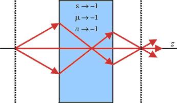
51 What is a metamaterial? Engineered materials, designed to have unusual properties Periodic structures Resonant inclusions Negative refractive index Negative or near zero permittivity/permeability 48 / 53

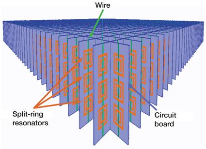
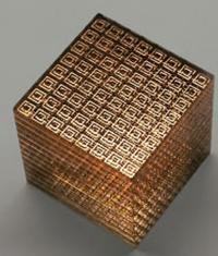
52 Some examples 49 / 53

53 Typical frequency behavior of a dielectric ɛ = ɛ jɛ ɛ(0) + conduction + + vibration rotation + transition relaxation ɛ( ) f (Hz) 50 / 53

54 Typical frequency behavior of a dielectric ɛ = ɛ jɛ ɛ(0) + conduction + + vibration rotation + transition relaxation ɛ( ) f (Hz) Between the low- and high-frequency asymptotes ɛ(0) and ɛ( ) (green region), there are no bandwidth limitations for metamaterial design. Outside the asymptotes there are strong restrictions on bandwidth for metamaterials (note small dip at f Hz). 50 / 53

55 Bounds on metamaterials The requirements of linearity, causality, time translational invariance, and passivity, gives bounds on the relative bandwidth B (after some complex analysis involving Kramers-Kronig relations). max ɛ(ω) ɛ m ω B B 1 + B/2 (ɛ ɛ m ) { 1/2 lossy case 1 lossless case 51 / 53

56 Outline 1 Harmonic time dependence 2 Constitutive relations, time domain 3 Constitutive relations, frequency domain 4 Examples of material models 5 Bounds on metamaterials 6 Conclusions 52 / 53

57 Conclusions Constitutive relations are necessary in order to fully solve Maxwell s equations. Their form is restricted by physical principles such as linearity, causality, time translational invariance, and passivity. A Debye model is suitable for dipoles aligning with an imposed field (relaxation model). A Lorentz model is suitable for bound charges (resonance model). There are restrictions on what kind of frequency behavior is physically possible. If you want extreme behavior (outside lowand high-frequency asymptotes), you get small bandwidth. 53 / 53