Evaluation of FWD software and deflection basin for airport pavements

Transcription

1 University of New Mexico UNM Digital Repository Civil Engineering ETDs Engineering ETDs Evaluation of FWD software and deflection basin for airport pavements Mesbah Uddin Ahmed Follow this and additional works at: Recommended Citation Ahmed, Mesbah Uddin. "Evaluation of FWD software and deflection basin for airport pavements." (21). This Thesis is brought to you for free and open access by the Engineering ETDs at UNM Digital Repository. It has been accepted for inclusion in Civil Engineering ETDs by an authorized administrator of UNM Digital Repository. For more information, please contact

2

3 EVALUATION OF FWD SOFTWARE AND DEFLECTION BASIN FOR AIRPORT PAVEMENTS BY MESBAH UDDIN AHMED B. Sc. in Civil Engineering Bangladesh University of Engineering and Technology, Dhaka, Bangladesh THESIS Submitted in Partial Fulfillment of the Requirements for the Degree of MASTER OF SCIENCE Civil Engineering The University of New Mexico Albuquerque, New Mexico July, 21 ii

4 21, Mesbah Uddin Ahmed iii

5 DEDICATION To my parents iv

6 AKNOWLEDGEMENTS I would like to thank Dr. Rafiqul A. Tarefder, my supervisor and thesis committee chair, for his support, time and encouragement for this study. His guidance and professional style will remain with me as I continue my career. I would like to thank my thesis committee members: Dr. Tang-Tat Ng and Dr. John C. Stormont for their valuable recommendations pertaining to this study. I would like to express my gratitude to the Aviation Department, New Mexico Department of Transportation (NMDOT) for the funding to pursue this research. I would like to thank Jane Lucero, Administrator, Aviation Department and Robert McCoy of Material Bureau, NMDOT for their assistance in field data collection. Co-operation and encouragement from the team members of my research group are highly appreciated. I thank Raju Bisht and Ryan W. Webb for their sincere effort in laboratory testing for this study. Motivation from my friend, a graduate student Late Mohammad Minhaz Mahdi is greatly acknowledged. v

7 EVALUATION OF FWD SOFTWARE AND DEFLECTION BASIN FOR AIRPORT PAVEMENTS BY MESBAH UDDIN AHMED ABSTRACT OF THESIS Submitted in Partial Fulfillment of the Requirements for the Degree of MASTER OF SCIENCE Civil Engineering The University of New Mexico Albuquerque, New Mexico July 21 vi

8 EVALUATION OF FWD SOFTWARE AND DEFLECTION BASIN FOR AIRPORT PAVEMENTS by Mesbah Uddin Ahmed M. Sc. in Civil Engineering, University of New Mexico Albuquerque, NM, USA 21 B. Sc. in Civil Engineering, Bangladesh University of Engineering and Technology Dhaka, Bangladesh 27 ABSTRACT Falling Weight Deflectometer (FWD) test data are processed by backcalculation software to obtain modulus of layer materials of airport pavements. Currently, several backcalculation software are available. However it is not known which software produces accurate and consistence modulus values. In this study three backcalculation software; namely, BAKFAA, EVERCALC, and MODULUS are evaluated for consistency and accuracy. To examine accuracy, software predicted modulus values are compared to the laboratory tested modulus values of soils, aggregate, and asphalts. Consistency is examined by statistical analysis using three sets of FWD deflection data produced by three loads with magnitudes of 9, 12, and 16 kip at an identical location of an airport pavement. It is shown that EVERCALC software produces more consistent and accurate modulus values than the BAKFAA and MODULUS software. A concern with the available backcalculation software is that their analysis algorithms are based on layered elastic theory with linear materials models. In addition, they consider static loading, which is not the true representation of the dynamic loads applied in a FWD vii

9 test in the field. To this end, this study performs a dynamic analysis of the FWD deflection basin using a finite element method (FEM) with the consideration of nonlinear materials models. Results show that FEM predicted deflections have similar trends of the field measured deflections. However, a number of trial combinations of inputs and FEM models may be required to produce an identical match between the predicted and measured deflections. It is recommended that this approach be the subject of future studies. viii

10 TABLE OF CONTENTS ABSTRACT... vii CHAPTER INTRODUCTION Introduction Problem Statement Hypothesis Objectives...4 CHAPTER LITERATURE REVIEW Introduction FWD Test KUAB FWD Dynatest FWD Carl Bro FWD JILS FWD Current Applications of FWD test Backcalculation of Layer Moduli Boussinesq s Solution Method Multi-Layered Elastic Theory Finite Element Method Overview of Backcalculation Software BISDEF BOUSDEF CHEVDEF ISSEM ELMOD ELSEDEF...19 ix

11 2.5.7 LOADRATE MODCOMP OAF FWD AREA SEARCH WESDEF VESYS Research Background...22 CHAPTER BACKCALCULATION METHODOLOGY Introduction Principle of Backcalculation FAA Guidelines for Backcalculation Data Collection Factors Responsible for Analysis Anomalies Analysis Review of Backcalculated Modulus Backcalculation Software BAKFAA MODULUS EVERCALC AASHTO Factors Affecting Backcalculated Modulus Loading Climate Pavement Condition Backcalculation in Airport Pavement Evaluation Summary...45 CHAPTER ACCURACY AND CONSISTENCY x

12 4.1 Introduction Objectives Study Approach Data Collection and Testing Plan FWD Testing Asphalt Coring and Soil Sampling in the Field Laboratory Testing Resilient Modulus of Asphalt Concrete Indirect Tensile Strength of Asphalt Concrete Consistency of the Software Frequency Plot of M r Frequency Plot of CV of M r Accuracy of the Software Backcalculated vs. Measured Modulus of Asphalt Concrete Backcalculated vs. Measured Modulus of Subgrade Backcalculated vs. Measured Tensile Strength of Asphalt Concrete Conclusion...69 CHAPTER FINITE ELEMENT MODELING OF FWD DEFLECTION Introduction Objectives FEM Model Description Model Geometry Layer Property Meshing of Model Boundary Condition Loading Criteria Finite Element Analysis Static Analysis Dynamic Analysis...11 xi

13 5.5 Discussion Static Deflection Basin Dynamic Deflection Basin and Time History Deflection at Layer Contour of Vertical Deflection Contour of Stress Comparing Static vs. Dynamic Analysis Conclusions CHAPTER CONCLUSIONS REFERENCES APPENDICES xii

14 LIST OF TABLES Table 3.1: FWD test plan Table 4.1: Borehole information in Runway 2-2 (Raton municipal airport) Table 4.2: Thicknesses of the Layers and Subgrade Soil Classification Table 4.3: Resilient Modulus and Indirect Tensile Strength of Asphalt Core Table 4.4: CV of a test location (MP 6 ft.) at Runway 8-26 at Silvercity Airport Table 5.1: Modulus of elasticity of flexible pavement layer Table 5.2: Parameters of the finite element model Table 5.3: Vertical deflection at the layer interface xiii

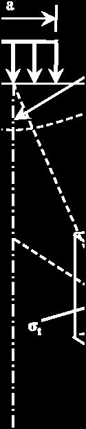
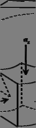
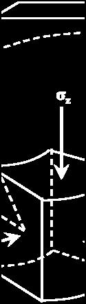
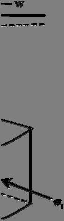
15 LIST OF FIGURES Figure 2.1: FWD test and the pavement surface response Figure 2.2: Generalized pavement response under uniformly distributed load (Boussisnesq, 1885) Figure 2.3: Multi-layered pavement structure... 3 Figure 3.1: Flow chart of the backcalculation of layer moduli Figure 3.2: Different types of anomalies in deflection type Figure 3.3: Rigid layer depth determination... 5 Figure 3.4: Generalized plan of FWD test Figure 3.5: Layer thickness consideration for the analysis Figure 4.1: Data collection Raton Municipal Airport Figure 4.2: Laboratory resilient modulus and Indirect tensile strength test Figure 4.3: Frequency distribution of the surface modulus Figure 4.4: Frequency distribution of base modulus Figure 4.5: Frequency distribution subgrade modulus Figure 4.6: Frequency distribution of coefficient of variation of the analysis... 8 Figure 4.7: Backcalculated surface modulus vs. Laboratory resilient modulus (9 kip load) Figure 4.8: Backcalculated surface modulus vs. Laboratory resilient modulus Figure 4.9: Backcalculated modulus vs. Subgrade modulus for accuracy Figure 4.1: Tensile stress developed at the bottom of the surface course Figure 4.11: Backcalculated vs. Laboratory tensile strength Figure 5.1: The zone of influence during FWD test Figure 5.2: Qualitative diagram of the Axi-symmetric model of flexible pavement Figure 5.3: Qualitative diagram of the Quarter cube model of flexible pavement Figure 5.4: Stress-strain distribution of the granular soil in base course (Garg and Thompson, 1997) xiv

16 Figure 5.5: Stress-strain distribution of subgrade soil from triaxial test (Slope stability 23) Figure 5.6: Mesh refinement of the axi-symmetric model Figure 5.7: Mesh refinement of the quarter cube model Figure 5.8: Amplitude pattern of the impulse in the FWD test Figure 5.9: Time-deflection histories of the sensors Figure 5.1: Deflection basins analyzed for different layer moduli combinations (axi-symmetric static analysis) Figure 5.1: Deflection basins analyzed for different layer moduli combinations (axi-symmetric static analysis) Figure 5.11: Deflection basins analyzed for different layer moduli combinations (quarter cube static analysis) Figure 5.11: Deflection basins analyzed for different layer moduli combinations (quarter cube static analysis) Figure 5.12: Deflection basins analyzed for different layer moduli combinations (axi-symmetric dynamic analysis) Figure 5.12: Deflection basins analyzed for different layer moduli combinations (axi-symmetric dynamic analysis) Figure 5.13: Time-deflection histories at the sensors for layer moduli combinations (axisymmetric dynamic analysis) Figure 5.13: Time-deflection histories at the sensors for layer moduli combinations (axisymmetric dynamic analysis) Figure 5.14: Deflection basins analyzed for different layer moduli combinations (quarter cube dynamic analysis) Figure 5.14: Deflection basins analyzed for different layer moduli combinations (quarter cube dynamic analysis) Figure 5.15: Time-deflection histories at the sensors for layer moduli combinations (quarter cube dynamic analysis) Figure 5.15: Time-deflection histories at the sensors for layer moduli combinations (quarter cube dynamic analysis) Figure 5.16: Contour of vertical deflection (2, 4, and 8 ksi) Figure 5.17: Contour of vertical deflection (3, 4, and 24 ksi) xv

17 Figure 5.18: Contour of vertical deflection (2, 4, and 8 ksi) Figure 5.19: Contour of vertical deflection (3, 4, and 24 ksi) Figure 5.2: Contour of von Mises stress (2, 4, and 8 ksi) Figure 5.21: Contour of von Mises stress (3, 4, and 24 ksi) Figure 5.22: Contour of von Mises stress (2, 4, and 8 ksi) Figure 5.23: Contour of von Mises stress (3, 4, and 24 ksi) Figure 5.24: Comparison of FWD deflection basins (axi-symmetric) Figure 5.24: Comparison of FWD deflection basins (axi-symmetric) Figure 5.25: Comparison of FWD deflection basins (quarter cube) Figure 5.25: Comparison of FWD deflection basins (quarter cube) xvi

18 CHAPTER 1 INTRODUCTION 1.1 Introduction Falling Weight Deflectometer (FWD) is a widely used nondestructive test to measure the pavement surface deflection for the evaluation of pavement structural capacity. In this test, an impulse is generated on the surface by dropping a weight from a pre-defined height. The load is then transmitted to the pavement through a circular steel plate. In response to the applied load, the pavement surface moves vertically downward and thus, forms a deflection basin. Geophones located at different offsets from loading point measure these vertical deflections. These deflection data are then processed to evaluate the pavement strength in terms of layer modulus. This layer modulus determined from known FWD data is termed as backcalculated modulus. A number of commercial and non-commercial software are available for the analysis of FWD data to obtain backcalculated layer modulus. The backcalculated modulus is not only used in design but also to determine the remaining life of the pavement, thus, the role of this layer modulus is significant in pavement engineering. This study focuses on the evaluation of the backcalculated layer modulus. 1.2 Problem Statement The available backcalculation software have some drawbacks in determining backcalculated modulus. Limited study was done before on these aspects. To date, a rigorous study has not been carried out to evaluate the backcalculated modulus. 1

19 Accuracy is one of the limitations of the backcalculated modulus from these software. It is necessary for the backcalculated moduli to be the same or very close to the laboratory test data. If the backcalculated modulus is higher than the laboratory determined modulus, it will lead towards the under-design of the pavement. Conversely, the lower backcalculated modulus may result in over-design of the pavement thickness, and the resulting design will not be economical. To forecast the remaining life of a pavement, the accuracy of the backcalculated modulus plays a significant role. A backcalculated modulus that is greater than the actual modulus will result in the predicted remaining life being greater than the actual life. If necessary maintenance is not applied, the overlay design will not be adequate to provide the pavement with necessary structural capacity. On the other hand, a backcalculated modulus that is lower than the actual modulus will result in a shorter predicted remaining life. Consequently, the design produces a maintenance cost greater than actually required. Therefore, it is necessary to examine the accuracy of the backcalculation software. Another problem associated with the backcalculation software is the lack of consistency of the results in that backcalculated moduli determined using different loads are not the same. According to the requirements of ASTM D 4694, different magnitudes of loads are applied in FWD test. The backcalculated moduli at a test section should be the same or at least very close to each other for different load levels. If the differences between the backcalculated moduli from the software are significant, the software can be considered to have a lack of consistency. The lack of consistency raises the question about the applicability of the backcalculated layer modulus. So, it is important to understand on the consistency of the backcalculation software. 2

20 Most commercial software is based on the layered elastic analysis. Some software packages have the option to integrate 2D Finite Element Modeling (FEM) of pavement into the analysis. There are also a few non-commercial software uses the 3D finite element modeling in the analysis of FWD data. Most of the 3D finite element modeling considers the FWD loading to be static. However, the FWD test load is not the static. The load applied in the FWD test is dynamic, that is, the load varies with time. For the 3D modeling of the flexible pavement with dynamic load, some of the studies consider the haversine load applied on the pavement surface (Lukanen 1993, Hoffman 1983, Nazarian 1995, and Sebaaly et al 1986). However, this is not a true representation of the FWD load. Therefore, the time-deflection history determined from those modeling may not be appropriate for the FWD data analysis. This suggests the application of 3D finite modeling requires more understanding. 1.3 Hypothesis A number of commercial software has the lack in accuracy and/or consistency of the backcalculated modulus. The applicability of these backcalculated layer moduli needs to be evaluated. For comparison to the backcalculated modulus from these software, moduli were determined from laboratory tests conducted on asphalt concrete samples collected from airport pavements. To investigate the consistency of the backcalculated modulus, the statistical analysis is done in this study. The 3D finite element modelings of the flexible pavement in the previous studies have considered the dynamic load with the haversine load pattern. This loading pattern does not represent loading measured in the field (Nazarian 1995). Therefore, the results from 3

21 these analyses were not good enough to represent the field response. For this reason, this study focuses on the 3D finite element modeling of FWD deflection basin with an impulse dynamic load. The response of the pavement is determined in terms of timedeflection history, i.e., the deflection varies with time at each sensor (geophone). The time-deflection history from this model can be used for the backcalculation of the layer modulus. 1.4 Objectives The first hypothesis has recommended some objectives and these are: - Analyze FWD data to backcalculate modulus using different backcalculation software. - Perform laboratory tests for determining resilient modulus and indirect tensile strength of the asphalt concrete. Compare the analysis results with the laboratory test data to check the accuracy of the software. - Compare the backcalculated modulus for a single point at three different loads to evaluate the consistency of their analysis. A number of researchers used the MODULUS and EVERCALC for their study (Ameri et al 29, Yin and Mrawira 29, Rahim and George 23, and Mahoney et al 1989) and these are widely used for the strength evaluation in highway pavement. Federal Aviation Administration (FAA) developed a backcalculation software BAKFAA to process the FWD data from airport pavement (Larkin and Hayhoe 29). For this reason, three software MODULUS 6., EVERCALC 5., and BAKFAA are used in this study. 4

22 The objectives under the second hypothesis are: - To generate the time-deflection histories at the sensor points of the flexible pavement under the impulse during the FWD test using 3D Finite Element Method. - To study the variations of the time-deflection history with the variations in layer properties, thickness, and the depth to rigid layer. - To perform static analysis and observe the deviation of the analysis results from dynamic analysis. 5

23 CHAPTER 2 LITERATURE REVIEW 2.1 Introduction FWD test for the pavement strength evaluation plays an important role in the pavement engineering since its inception in early 198 s. Since then, several methods have been developed for the investigation of the structural capacity of the pavement layers using FWD data. This chapter focuses on the current practices of the pavement strength evaluation by FWD test, the data processing methods, and FWD s applicability in the pavement design and maintenance. A brief discussion of research regarding FWD data analysis methodologies and the pavement deflection modeling are covered in this chapter. 2.2 FWD Test In this test, an impulse load is generated on the pavement surface by dropping a weight on a circular plate of 12 to 18 in. diameter from a height of 1.5 to 2 ft using a spring-mass system. The duration of the load is about 2 to 35 milliseconds. The steel plate comes to a smooth contact with the surface of the pavement by the use of a rubber pad. Pavement deflections are measured by seven geophones resting longitudinally on the surface. A photograph taken during initial setup of the FWD testing assembly is shown in Figure 2.1(a). Due to the application of the dynamic load, the pavement surface deflects vertically downward forming a deflection basin. Figure 2.1(b) is a schematic of a deflection basin. The FWD device can accommodate seven to nine sensors for the measurement of vertical deflections. However, in this study seven geophones are used at different radial offset from the load. The distances of the geophones from the center of 6

24 the loading plate are, 8, 12, 18, 24, 36, and 6 inches (AC 15/537-11A). The sensor at inch distance means the surface deflection at the loading point. The magnitudes of the load are varied at three load levels of 9, 12, and 16 kips. For each load, two replicate tests are performed at a single test point or location. FWD test was carried out in accordance with the ASTM D There are different manufacturers of impulse devices. They are KUAB America, Dynatest Group, Carl Bro Group and Foundation Mechanics Incorporated KUAB FWD KUAB FWD includes five models with load ranges up to 66 kips ( KN). The load is applied through a two mass system and the dynamic response is measured with seismometers and LVDT s through a mass-spring reference system. There is a load plate to produce uniform pressure on the pavement surface Dynatest FWD Dynatest FWD generates dynamic loads up to 54, pounds (24.2 KN). The weights are dropped onto a rubber buffer system. Seven to nine velocity transducers are used to measure the load and dynamic response Carl Bro FWD Carl Bro FWD generates dynamic loads up to 56, pounds (249.1 KN). The FWD uses 9 to 12 velocity transducers to measure load and dynamic response. Weights are dropped on a rubber buffer system and the load plates are four-split allowing maximum contact to the surface measured upon. 7

25 2.2.4 JILS FWD Foundation Mechanics manufactures JILS FWD. These can generate loads from 1,5 pounds (6.67 KN) to 54, pounds (24.2 KN). The FWD uses two mass elements and a four spring set combination to impose a force impulse in the shape of a half-sine wave. Load magnitude, duration and rise time are dependent on the mass, mass drop height and arresting spring properties. Seven velocity transducers are used to measure the deflection. In this study, the data are collected from JILS FWD 2T since the NMDOT-Aviation department uses this nondestructive device in the evaluation of airport pavement. 2.3 Current Applications of FWD test The goal of the FWD data is to investigate the present structural capacity of the pavement. The structural capacity of the pavement is determined by the parameters calculated from the deflection data in FWD test. The deflection data are mainly collected under a certain magnitude of the FWD load and thus, the pavement layer strength is measured from this test. Current practices of the pavement strength evaluation by FWD test include: The allowable deflection is determined based on the past performance of the pavement under the FWD test. Then, whenever the test is repeated at the same section of the pavement, the measured deflection is compared with allowable deflection. The pavement is workable under the load if this measured deflection is greater than the allowable and vice versa. Comparison of measured behavior against calculated allowable criteria. These criteria determined by elastic layer analysis and usually in terms of deflection. 8

26 The remaining life of the pavement is determined by the existing design method. Another way is to determine the load carrying capacity. This capacity is calculated from the deflection data in FWD test. The layer strength is calculated from the FWD data and the layer thicknesses of the pavement. This layer strength is expressed in terms of backcalculated modulus of pavement layer. Combination methods using laboratory material test results in conjunction with the backcalculation procedure to provide material properties required for a theoretical analysis of fatigue and measured behavior to provide limiting criteria. The first three methods are used widely under limited testing conditions. They cannot relate the variations in material, environment and load limit. The last two methods are able to give a more general solution to the structural evaluation problem. Though still now, they are not easy to implement due to the inherent limitations of the currently available mechanistic pavement analysis model. 2.4 Backcalculation of Layer Moduli Backcalculation of the layer moduli is the most widely accepted method for the interpretation of the structural capacity of the pavement from the FWD data (Rahim and Geprge 23, and Romanoschi and Metcalf 1999). Backcalculation requires inputs such as number of layers, layer thicknesses, Poisson s ratio of each layer, temperature, and the presence of rigid layer underneath the subgrade. Prior to the analysis, the layer modulus is assumed initially that is often called seed modulus. The surface deflections at radial offsets (geophone location) are calculated by the mechanistic analysis using the seed 9

27 modulus and layer geometry. These surface deflections at radial offsets form a deflection basin. The calculated deflections are then compared to the field measured deflections. The process is repeated by changing the (seed) moduli each time, until the difference between the calculated and measured deflections are within a selected tolerance or limit value. As a part of the backcalculation procedure, the surface deflection at the points located at different distances from the loading point need to be determined with the available mechanistic analysis. Generally, three methods are mostly used in the most of the backcalculation algorithm and they are: Boussinesq s solution method. Multi-layered elastic theory. Finite element model Boussinesq s Solution Method Boussinesq (1885) proposed some mathematical relations to characterize the response of the soil under the load imposed by a structure. These relationships can calculate the stress, strain, and the deflection of the pavement under a concentrated load. These are based on some basic assumptions that the pavement is a homogenous, isotropic, and linear elastic semi-infinite space. However, the pavement in real field is not subjected to the point load and to date this problem, the point loads are then integrated to a uniformly distributed load. And the pavement is also assumed as an axi-symmetric structure for the formulation of the pavement response. The equations are mentioned below: 1

28 where, vertical deflection, circular load, modulus of elasticity, Poisson s ratio, radius of the circular area, and depth at the reference point. Figure 2.2 shows the generalized stress-strain response diagram of the pavement under a uniformly distributed load. Boussinesq s equations are valid only for the single layer of isotropic, homogenous layer property. However, the pavement is a layered structure with different material properties. Odemark (1943) proposed a layer transformation method that makes Boussinesq s equations applicable to the analysis of multilayered pavement structure. The principle of this method is to transform a system consisting of layers with different moduli into an equivalent system where all layers have the same modulus. The method is also known as the method of equivalent thickness (MET). The relationship for the layer transformation is mentioned below:

29 Where, equivalent thickness of the first layer to the second layer, thickness of the first layer, thickness of the second layer, modulus of elasticity of the first layer, modulus of elasticity of the second layer, Poisson s ratio of the first layer, Poisson s ratio of the second layer, and correction factor (usually.8 for multi layered system except at the interface of the first layer). The whole structure is then transformed into a single layer structure of homogenous and isotropic layer property to determine the pavement response using the Boussinesq s solution Multi-Layered Elastic Theory Flexible pavement is multi-layer structure, as mentioned in Figure 2.3, with stronger materials on top and it is accurately represented by a homogenous mass (Huang 24). To characterize the pavement response under a load, Burmister (1943) first proposed solutions for the two-layer system and then extended them to a three-layer system (Burmister 1945). With the advances in computation efficiency, it can be applied to any number of layers (Huang 1968). The assumptions of the layered theory are mentioned below: The pavement system consists of several members, each made of a different material. Each member is of uniform thickness and infinite dimensions in all horizontal directions (Burmister layer), resting on a semi-infinite elastic and isotropic domain (Boussinesq half space). Each member consists of a homogenous, isotropic, linear, and elastic material whose constitutive equation is governed by Hooke s law. 12

30 The system is free of any stress and deformations, before application of external traffic loading. There is no body force acting in the system. To implement this theory, it includes the following steps: Governing Equations The solution of the problem related to the multi layered pavement structure is known as boundary value problem. The following equations are the main during the implementation of this theory: Equilibrium equations. Compatibility equations. Constitutive law. Boundary conditions. The multilayer solution system is developed using the first three equations and it is solved by applying the boundary condition. Formulation of the theory The equilibrium equation, compatibility equation and the constitutive law for a continuum can be expressed in Cartesian coordinates as below (Timoshenko and Goodier 197): Equilibrium equation:, 2.6 Compatibility equation:,,

31 Constitutive law: 2.8 where, Cauchy stress tensor, Cauchy strain tensor, displacement tensor, Kronecker delta, Young s modulus of material, and Poisson s ratio. For an axi-symmetric solid, the stress and displacements can be written in the polar coordinate as below: In axi-symmetric problem, the following displacement and the stresses are zero: ; 2.11 The stress and displacement components can now be rewritten in terms of the biharmonic stress function, (Love 1927):

32 The function,, is evaluated by applying the boundary condition. From these equations, only the vertical deflection (w) relationship is used in the backcalculation procedure. The application of the multi-layered elastic method is simple and fast in the computation of the pavement response. However, it has some limitations to represent the true behavior of the field situation. In this theory, all the layers are horizontally infinite that is not possible in any pavement section Finite Element Method Finite element method to characterize the pavement response is very useful to address the limitations of the multi-layered solution method. It can work with different shape and geometry as well as with different material types. The steps that are involved in this method are mentioned below: The shape and geometry of the pavement is assumed, i.e. structure with different layers and thicknesses. The material property for each layer needs to be assigned, i.e. the strength and other properties of the layer material. The boundary conditions of the structure are to be assumed according to the field condition, i.e. the load and support conditions imposed on the pavement geometry. 15

33 The geometry is to be discretized with grid to make the whole model is the summation of a number of unit elements, i.e. mesh the geometry. The potential energy function for the single element or cell has to be developed. Minimize the function to get the stiffness matrix of each element in its local coordinate. The stiffness matrices for the elements in their local coordinate are then assembled to get the global stiffness matrix of the whole structure. The boundary conditions need to be applied to get the pavement response. The finite element model of the pavement is also used to determine the surface deflection at different sensor locations. The 2D model is used a lot in the backcalculation method and some commercial software has the option to use this 2D FEM. A number of researches are underway to investigate the proper pavement response with 3D FEM. 2.5 Overview of Backcalculation Software BISDEF BISDEF is developed by the U.S. Army Corps of Engineers, Waterways Experiment Station. It uses a deflection basin from NDT results to predict the elastic moduli of upto four pavement layers. It uses an iterative process that provides the best fit between measured deflection and computed deflection basins. The assumption is that dynamic deflections correspond to those predicted from the elastic layer theory. The program uses the BISAR layered elastic program to calculate the deflections, stresses and strains of the structures under investigation. It can vary the bond between the layers in the pavement. For this reason, the run time of this program is long. For determining the layer moduli, 16

34 some parameters of the pavement are given as the basic input. These parameters include thickness of each layer, range of allowable modulus, initial estimates of modulus and poisson ratios BOUSDEF BOUSDEF is a backcalculation program to determine the in-situ pavement layer moduli using deflection data through backcalculation technique. It was created by Oregon State University. The analysis methodology of this program is based on the method of equivalent thickness and Boussinesq theory. It utilizes the seed modulus and layer thickness for calculating the equivalent thickness of the pavement structure. Then, for a given NDT load and load radius, the deflections are calculated. The calculated deflections are compared to in-situ deflections. The sum of the differences between these two sets of deflection is determined. If the sum is greater than the tolerance specified by the user, it will start the iteration. The purpose of the iteration is to converge the difference between these deflections. This is done by changing the moduli to get a new set of deflection. It will continue until the difference is less than the tolerance. After that, the backcalculated moduli can be used for two purposes. First, evaluation of the structural capacity of the pavement and second, during the mechanistic overlay design. This program was developed for the conventional flexible pavement consists of fine grained subgrade with coarse grained aggregate base/subbase CHEVDEF CHEVDEF is similar to BISDEF. The difference is that it uses CHEVRON n-layer computer program in the forward calculation scheme. To meet the convergence criteria, 17

35 BISDEF uses the sum of the differences of the deflections where CHEVDEF uses the sum of the squares of the differences. This program is able to give reasonable value for the pavement sections having stiffness decreasing with depth. For the pavements with thin HMA layers or intermediate hard or soft layers such as cement stabilized bases or subbases, it gives poor result ISSEM4 ISSEM4 is a mechanistic pavement analysis computer program. It is based on ELSYM5. It uses an iterative procedure of matching the measured surface deflections with the surface deflections calculated from ELSYM5 using assumed elastic moduli. This is applicable for three layered pavement structures. It uses five deflection points in the backcalculation process ELMOD ELMOD is developed by Odemark. It uses the method of equivalent thicknesses. Here, the layered pavement structure is transformed into an equivalent Boussinesq system above the subgrade. It uses the layer transformation approximation. The advantages of this approach are that the material non linearity can be considered here and the computation is faster than conventional layered elastic analysis. The inputs of this program include layer thicknesses and pavement surface deflections. It is able to analyze up to a four layered pavement structure. For each FWD drop, it calculates the subgrade nonlinear-stress relationship. During backcalcualtion, first, it calculates the subgrade modulus by using the outer deflections. Using the center deflection and the shape of the deflection basin, the moduli of the HMA and base courses are determined. The subgrade 18

36 modulus at the center of the load plate is then adjusted for stress level and the outer deflections are checked. A new iteration is made, if needed, at this stage. This program is able to determine the remaining life and required overlay thickness ELSEDEF ELSEDEF is similar to BISDEF, but the difference is that ELSEDEF uses ELSYM5 as an elastic layer program. It also uses the iterative procedure to determine the best fit between measured and computed deflections. The modulus adjustment process includes the determination of a relationship between log modulus and calculated deflection for each unknown modulus by varying the assumed moduli and calculating the deflections. Then, it is used in the iteration process to find a set of moduli with error minimization. The inputs of this program include the layer thicknesses, Poisson s ratio, load, deflection basin data, seed moduli and allowable range of moduli. The number of layers should be less than the number of measured deflections. It does not consider the material non linearity. It is not mandatory to consider the rigid layer for analysis. The choice of seed modulus affects the result LOADRATE LOADRATE program is developed for use with surface-treated pavements typical of secondary roads. It uses a series of regression equations between load and deflection based on results generated by ILLI-PAVE. These are developed to relate the nonlinear elastic parameters of the bulk stress model for base material and the deviator stress model for subgrade with the deflection at the center and some distance away from center. 19

37 2.5.8 MODCOMP2 MODCOMP2 uses the CHEVRON elastic layer program. It also uses the iterative procedure with an assumed set of seed moduli to backcalculate the modulus values of different layers of pavement. The iteration ends when the difference between the measured and calculated defections is less than the tolerance with a maximum number of iterations. The input of this program includes surface deflection and radial distances of geophones from the center of the load, applied load, Poisson s ratio, base and subgrade soil type and seed modulus for the pavement layers. It can analyze the pavement of up to eight layers. The layer combination may be linear elastic or nonlinear stress dependent. It can work with the data obtained from several NDT devices like FWD, Road Rater and Dynaflect. It can accept up to six load levels OAF OAF is developed to analyze the data from the FWD. The deflections at, 3, 6 and 1 cm from the applied load are used in this program. It uses ELSYM program to calculate surface deflections. The inputs are surface deflection measurements and load configuration, base type, layer thicknesses, Poisson s ratio for all layers and HMA modulus at field temperature. The moduli are calculated by attaining the compatibility between measured and calculated deflections FWD AREA FWD AREA is developed by Washington State Department of Transportation. This program is useful in calculating normalized and temperature adjusted deflections, area value and subgrade moduli from FWD data collected using Dynatest FWD (Version 2). 2

38 For the determination of subgrade modulus it uses the AASHTO the relationship between the resilient modulus and deflection. The processed data contains the station or milepost location, all testing load levels, corresponding deflections at each sensor, normalized deflections to 9 lbs (4 KN), normalized and adjusted (for temperature) center deflection, normalized and adjusted area value and normalized subgrade modulus SEARCH SEARCH uses a pattern-search technique to match deflection basins with curves shaped like elliptic integral functions which represent solutions to the differential equations used in elastic layer theory. It is developed at the Texas Transportation Institute. In case of multiple layers, a generalized form of Odemark s assumption is used to transform the thickness of all layers to an equivalent thickness of a material having a single modulus. The input of this program includes thickness of HMA and granular base layers, applied force and radius of load plate and measured deflection values and their radial distances from the center of loading. It determines the set of moduli that fit the measured basin to the calculated basin with the last average error. The output includes calculated moduli, computed and measured deflections, force applied and squared error of the fitted basin WESDEF WESDEF is developed by the U.S. Army Corps of Engineers, Waterways Experiment Station. It can calculate modulus values for one set of deflections and multiple loads. The deflection can be entered manually by INDEF. The assumption of this program is that dynamic deflections correspond to those predicted from the same loads using static layered elastic theory. It uses the WES5 layered elastic program for calculating the 21

39 pavement structure. It also uses the iteration procedure to fit the measured deflection with computed deflection by varying the moduli VESYS VESYS is used to develop a graphical procedure for backcalculating the pavement parameters.it considers the viscoelastic and fatigue properties of the pavement materials. The load deflection data and known material thickness or properties are used for the analysis of the existing pavement. The algorithm for this program is developed by applying statistical regression analysis technique to the VESYS generated response data. There are four other backcalculation software/ algorithm and they are MODULUS 6., EVERCALC 5., BAKFAA, and AASHTO 1993 backcalculation algorithm. The first two software are the most used software now a day. BAKFAA is still under improvement and the last one is the backcalculation algorithm specified in the AASHTO The details of their backcalculation procedures will be described in the next chapter. 2.6 Research Background The influence of the backcalculated layer moduli is pronounced in both design and maintenance of the pavement. Lack of accuracy and consistency may result in underdesign or overdesign. Therefore, the applicability of the backcalculation algorithm is one of the major issues in pavement engineering. Ameri et al. (29) performed a comparative study on four software, MODULUS 6., ELMOD 5., EVERCALC 5., and Dynamic Backcalculation with System Identification (DBSID). The DBSID is a dynamic analysis backcalculation software and the others are static analysis software. In static analysis, the surface deflection at each offset is assumed to be function of the modulus of 22

40 elasticity at a specified depth (William 1999, Huang 24). To check the accuracy of the analysis, Ameri et al. (29) compared the backcalculated subgrade modulus to subgrade modulus determined by empirical relation. They determined the subgrade resilient modulus from California Bearing Ratio (CBR). The CBR value was determined from soil properties. They also observed the time needed for a single run of the analysis in these software. Based on accuracy of subgrade modulus and run-time efficiency, Ameri et al. (29) recommended MODULUS 6. to be the most appropriate software. Yin and Mrawira (29) carried out dynamic modulus test of asphalt concrete and correlated laboratory modulus to backcalculated modulus. They used ELMOD, EVERCALC, and MODULUS for the backcalculation of FWD data. They observed that the analysis results from ELMOD were in close agreement with laboratory test results. Ji et al. (26) developed spline semi-analytical method to determine pavement response and system identification method to backcalculate modulus. In the spline method, flexible pavement was considered to be a multi layered visco-elastic system. The analysis results were compared to the results from the two other backcalculation software namely, MICHBACK and DYNABACK-F. MICHBACK is static backcalculation software developed by the Michigan Department of Transportation and the University of Michigan Transportation Research Institute. DYNABACK-F is a dynamic analysis software. The spline results were in good agreement with the results from software. However, Ji et al. (26) study did not compare laboratory moduli but spline modulus to the backcalculated moduli. Mahoney et al. (1989) evaluated five backcalculation software: ELMOD, ELSDEF, EVERCALC, ISSEM4, and MODCOMP2. These authors indicated the reasons for 23

41 differences in the backcalculated moduli from these software are due to different number of deflections required for each software, differences in computational procedures, differences in seed moduli, and modulus limits, differences in deflections basin convergence subroutines of minimization algorithm and the acceptable tolerance in matching the calculated and measured deflection basin, and the ability to deal with nonlinear material response. They observed that backcalculated FWD modulus deviate from the laboratory modulus. The differences in stress states and load pulse durations between the laboratory and the FWD test were found to be the main reason for that deviation. Uddin and McCullough (1989) recommended the guideline to avoid the sources of errors associated with the deflection-basin matching techniques in FWD backcalculation. They used two software: FPEDD1 for asphalt pavement and RPEDD1 for rigid pavement. These authors used a methodology to generate seed moduli depending on the measured deflections and radial distances of the sensors. For reliable prediction of effective moduli from the deflection basins, they recommended several features of the self-iterative procedures such as appropriate structural response model, elimination of guessing the input moduli, correction of the backcalculated moduli for nonlinear behavior of granular layers and underlying soils, temperature correction for surface asphaltic concrete layer, and consideration of the effect of a rock layer in the analysis. For the improvement of the backcalculation procedure, research has been carried out involving the Finite Element modeling and pattern recognition. Gopalakrishnan (27) used artificial neural network (ANN) for predicting non-linear layer moduli of flexible airfield pavements subjected to new generation aircraft (NGA). This study was based on 24

42 the deflection basins obtained from heavy weight deflectometer (HWD) data. HWD tests were performed the Federal Aviation Administration s National Airport Pavement Test Facility (NAPTF) to monitor the effect of Boeing 777 (B777) and Boeing 747 (B747) test gear trafficking on the structural condition of flexible pavement sections. The pavement sections at NAPTF were modeled in ILLI-PAVE and synthetic database was generated for a range of moduli values. A multi-layer, feed-forward network with error-back propagation algorithm was trained to approximate the HWD backcalculation function using that database. The ILLI-PAVE synthetic database was used in the ANN training to account for the stress-hardening behavior of unbound granular materials and stresssoftening behavior of fine-grained subgrade soil. The model is able to predict the asphalt concrete (AC) and subgrade non-linear moduli from actual HWD field test data. This ANN-based rapid can enable analysis of a large number of HWD pavement deflection basins in real time, needed for routine airfield pavement evaluation. Wu et al. (26) used 3D layer spectral element to solve the problems of bounded layer system subjected to transient load pulse. Each layer of that system was treated as one spectral element. The wave propagation inside the layer was achieved by the superposition of the incident and the reflected wave. Fast Fourier Transformation (FFT) was used for transforming the Falling Weight Deflectometer (FWD) data from time domain to frequency domain and procedures from tome to frequency domain are done by Inverse FFT (IFFT). The system was solved by the summation over the frequencies and the wave numbers, which alleviated the inconvenience of the numerical calculation of infinite integration. The efficiency of this approach was verified by analyzing the FWD testing model with axi-symmetric spectral element program and 3D finite element 25

43 method. CAPA-3D was used as 3D finite element method and LAMDA was used as axisymmetric spectral element method. From this study it is found that, 3D layer spectral element method is more efficient than axi-symmetric spectral element program and 3D finite element method. Göktepe (24) applied multi layer perceptron (MLP) and adaptive neuro-fuzzy inference system (ANFIS) to backcalculate the mechanical properties of pavement layers. The objective of this study was to develop a methodology which would be able to perform real-time pavement analysis. During this study, the MLP and ANFIS were first trained. Once these were trained, backcalculation results from these two systems were compared to those obtained from the conventional backcalculation program MICH BACK. Nonlinear least-square estimator was used for comparison of the data. From the observations, ANFIS is able to deal with uncertainty using fuzzy logic. MLP is better choice if sufficient data is available for analysis. Both MLP and ANFIS do not use any physical principle, mechanical background and material behavior in analysis. Therefore, they can not replace the use of the conventional backcalculation program. Saltan (22) used the concept of NeuroFuzzy for the backcalculation of the pavement parameters. The objective of his study was to develop a method of analyzing the elastic modulus for different layers of pavement through surface deflections. These deflections were obtained from FWD test. The elastic analysis and finite element method are time consuming. This author wanted to reduce analysis time by the application of NeuroFuzzy. In this study, the deflection basin was modeled by finite element method including NeuroFuzzy. And the modeled deflection basin was almost the same as the measured set 26

44 of deflection. Therefore, it can be used as an applicable means to backcalculate the pavement parameters in a realistic manner within a short time. 27

45 Loading Assembly Deflection Sensor Loading Plate (a) FWD testing assembly (JILS FWD 2T) H Geophone D1 D2 Pavement Surface Deflection Basin Steel Plate Rubber pad Sensor Deflection (b) Schematic deflection basin of pavement surface Figure 2.1: FWD test and the pavement surface response 28

46 Figure 2.2: Generalized pavement response under uniformly distributed load (Boussisnesq, 1885) 29

47 q h 1, E 1, ν 1 h 2, E 2, ν 2 h n-1, E n-1, ν n-1 h n, E n, ν n Figure 2.3: Multi-layered pavement structure 3

48 CHAPTER 3 BACKCALCULATION METHODOLOGY 3.1 Introduction To perform backcalculation, it is necessary to know the details of each and every stage of the backcalculation process. The stages range from FWD data collection to review of the backcalculated layer moduli for the evaluation. This chapter mainly focuses on the implementation of the backcalculation process and the corresponding Federal Aviation Administration (FAA) guidelines, summary of the backcalculation software used in this study, and factors affecting the backcalculated modulus. 3.2 Principle of Backcalculation Backcalculation of the layer moduli is the interpretation of the pavement strength condition from the FWD test data. Therefore, it also involves some layer properties of the pavement to carry out the analysis. The layer properties cover the layer number and thicknesses, initially assumed modulus of elasticity and Poisson s ratio of each layer material, and pavement surface temperature. The reverse process of the determining the layer moduli from the FWD data as well as the pavement layer properties are the basic tasks of the backcalculation of moduli. The backcalculation procedure is described in the flow chart in Figure 3.1. The flow chart shows that the mechanistic analysis procedure, i.e. layered elastic analysis software, calculates the surface deflections at different radial offsets and then, these deflections are compared with FWD data. If the error (percent difference between the two sets of data) is within the specified tolerance, the initially assumed (seed) modulus set of the layers is considered to be the layer modulus of the 31

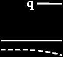
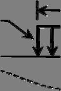
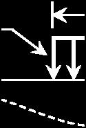
49 pavement. If it is not so, the whole process is repeated again with the corresponding change in layer moduli until the error is within the specified minimum value. 3.3 FAA Guidelines for Backcalculation Federal Aviation Administration (FAA) has given the guidelines for the backcalculation of the pavement layer modulus (AC No.: 15/537-11A). The goal of the backcalculation is to determine the pavement strength in terms of layer modulus so that the pavement structural capacity can be evaluated properly. The following are FAA analysis guidelines: Data Collection The data collection procedure involves the following steps: Surface Deflection The surface deflections are recorded from the FWD data under a certain amount of load application. These data are called deflection basin. Layer Information The detailed information of the layers can be recorded from the bore log and construction history. The bore log informs about the number of layers and the material of the individual layer. The information also includes the individual layer thickness. The initially assumed layer moduli and the Poisson s ratio are taken based upon the material type of the layer. 32

50 Temperature The FWD device records the pavement surface temperature at each station during the test in the site Factors Responsible for Analysis Anomalies The following factors may cause error during the analysis: Deflection Basin Anomalies The surface deflection is the maximum at the point of loading and it decreases gradually further from that point. Prior to the backcalculation process, it is mandatory to check the magnitude and shape of the deflection basin to observe whether there is any discontinuity in the deflections. Three types of anomalies are generally observed in the collected FWD data and they are: Type 1: The surface deflections at outer sensors are greater than the deflection at the loading point. This kind of discontinuity may be main cause of the highest error in the analysis. Figure 3.2(a) shows the deflection basin Type 1 anomaly. Here, in this figure it is seen that the deflection at the first sensor is 25 mils whereas the deflection is 3 mils at the second sensor. With the layered elastic analysis, it is not possible to get this shape of the deflection basin under the load and thus, there will be considerable error matching the calculated deflection basin with the field deflection basin. Type 2: The sharp change in the deflections between the two adjacent sensors may produce some erroneous analysis results. Figure 3.2(b) shows the deflection 33

51 basin with type 2 anomaly. The first sensor gives the deflection value of 6 mils whereas the second sensor gives the value of 28 mils and thus, results in steep jump in the deflection basin. Most of the backcalculation software integrates layered elastic analysis method for their analysis algorithm. According to this theory, the deflection decrease as the distance increases from the loading point and this decreasing pattern is gradual and relatively consistence among all the sensors. Type 3: The deflection at the outermost sensor of two adjacent sensors is greater than the deflection at the sensor that is closest to the load plate. Figure 3.2(c) shows the deflection with Type 3 anomaly. It is observed from the figure that the deflection at the sixth sensor is 5 mils and at seventh sensor, it is 9 mils. The sixth sensor value is greater than the seventh sensor value that is not possible to calculate with the layered theory. Therefore, the deflection basin matching process will also produce error in the analysis. Layer Parameters The flexible pavement usually has surface, base and sub-base over the subgrade. The first 6~12 inches of subgrade is engineered soil. Consideration of too many layers in the backcalculation with the help of layered elastic analysis may lead to error in the analysis. The decrease in layer thickness is another cause of increase the error in the analysis. The bond strength along the layer interface also affects the analysis. 34

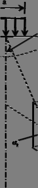
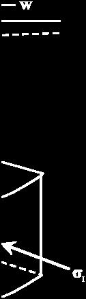
52 Temperature Asphalt concrete is sensitive to the temperature. The strength of the surface course gets reduced in the summer whereas the strength increases in winter. Therefore, temperature plays an important role in the backcalculation. Usually, a temperature correction factor is considered in a backcalculation software. Seed Modulus The initial set of modulus value that is selected for each layer may have an impact on the analysis. The magnitude of the error depends on the iteration algorithm that is used by the backcalculation software. Modulus Ratio The ratio of the modulus of elasticity of two adjacent layers. The analysis result is also affected by the adjacent layer modulus ratio. If the ratio is significantly high this may cause some error. Underlying Rigid/Stiff Layer The presence of the rigid/stiff layer at shallow depth causes a large error in the analysis if that layer is not considered. The effect is pronounced whenever the depth is less than 1 ft (3. m). The stiff layer does not need to be bedrock, it can be a layer that is much stiffer than the unbound layers above it. The depth to rigid layer has to be determined. The layer at the deeper depth is responsible for the deflection of the sensor located farther away from the loading point (Irwin 2). The vertical deflection at the interface of the subgrade-rigid layer is zero. Therefore, the radial distance where the vertical 35

53 displacement is zero is the depth to rigid layer (Irwin 2). Prior to backcalculation of the layer modulus, it is needed to determine this depth and thus, limit the thickness of the subgrade. Figure 3.3 shows the method of rigid layer depth prediction. From Figure 3.3(a), it is observed that the deflection of the sensor is reduced with the distance away from the load point and it is minimized at the farthest sensor. If the deflection basin is extended after the last sensor point, it will be zero at some radial offset as indicated in Figure 3.3(a). An arc of radius with same magnitude of the radial offset is then drawn. The depth at which that arc intersects the vertical line is the depth to rigid layer. The method of calculating this depth is shown in Figure 3.3(b). From the deflection basin developed from the FWD, the inverse of the sensor radial offset is determined at different locations. The displacements are then plotted against the inverse of the sensor radial offset at different locations. A tangent is drawn along the initial straight part of that curve. This tangent intersects x-axis at some point and this intercept is to be determined. The inverse of this x- axis intercept is the depth to rigid layer. Pavement Cracks The one of the assumptions behind layered elastic analysis is that each and every layer is infinite horizontally. Therefore, it does not consider any discontinuities in the layer of the pavement. If the load plate is near to this crack, the analysis result may have some error Analysis The collected data are investigated whether they satisfy the above mentioned requirements or not. If the data set meets all the requirements, it can be used for the 36

54 analysis as described previously. The available commercial software or closed formed solutions are able to backcalculate the layer moduli from the data Review of Backcalculated Modulus The applicability of the backcalculated modulus from the analysis should be reviewed according to the following requirements: The error limit (percent difference between the measured and determined deflections) will have to be within specified tolerance. The values of the layer modulus will have to be investigated whether these are reasonable or not. The modulus value for the individual layer should be checked whether this often hit the upper limit for each deflection basin. The modulus value for the individual layer should be checked whether this often hit the lower limit for each deflection basin. The modulus ratios between the adjacent layers should be investigated whether the values are realistic. The backcalculated modulus will be acceptable if the values satisfy the above mentioned requirements. 3.4 Backcalculation Software A number of commercial software is for backcalculation as mentioned previously. This study includes three software and one backcalculation algorithm from AASHTO The details of the software are described below: 37

55 3.4.1 BAKFAA BAKFAA is based on layered elastic analysis and employs a downhill multidimensional simplex minimization method for the backcalculation of layer moduli (Press et al. 27). The downhill multidimensional simplex minimization method is suitable for finding the minimum value of a function of more than one independent variable (Press et al. 27). BAKFAA calculates deflections at the specified points using the initial set of assumed layer moduli or seed moduli. Error minimization process involves determination of sum of the squares of differences between the FWD deflections and the deflections calculated by layered elastic analysis. BAKFAA is written in Visual Basic platform. BAKFAA can analyze a pavement having ten layers. However, BAKFAA cannot calculate the rigid layer depth and it does not account for temperature effect in modulus calculation. In BAKFAA, user has to assume the depth to rigid layer for the determination of subgrade thickness MODULUS 6. MODULUS 6. uses the Waterways Experiment Station Linear Elastic Analysis (WESLEA) method for forward calculation of moduli. WESLEA is developed based on the multilayer elasto-static theory. A database of deflection basins is generated for different modular ratio using WESLEA. It uses a pattern search technique to determine the set of layer moduli which produces a deflection basin that best matches with the field measured deflection (William 1999). It can analyze the pavement of maximum four layers. The rigid layer depth prediction is one of the advantages of this software. MODULUS assumes the radial distance to the point where the deflection is zero is 38

56 closely related to the rigid or stiff layer depth (Irwin 22). MODULUS software also accounts for the effect of temperature EVERCALC 5. EVERCALC 5. uses the WESLEA for the forward analysis. The forward analysis involves the calculation of surface deflections at the specified radial offsets using different combinations of initially assumed layer moduli. The calculated surface deflections are then compared to the field measured deflections. For each combination of layer moduli, the error between these calculated and measured moduli is determined. This step is repeated several times until the error is minimized. This process is known as the error minimization or optimization of solution. A modified Gauss-Newton algorithm is used for error minimization. FWD data from a maximum of ten sensors can be used and it can analyze twelve drops at each station. During the error minimization process, a trial is stopped whenever one of the following conditions is satisfied first (Everseries User Guide 25): - Deflection tolerance calculates deflection error between the field measured and the calculated deflections using the following formula: RMS % 1 n w w w

57 where RMS = root mean square of the error, w = field measured deflection during FWD test (mils), w = calculated deflection by the software (mils), m = number of sensors (maximum 1), and n = number of layers. - Moduli tolerance is based on the modulus difference between two consecutive iterations. The relationship of the moduli tolerance is shown below: e % E E E where e = percent difference of modulus between two consecutive iterations, E = i-th layer modulus at the k-th iteration, E = i-th layer modulus at the (k+1)-th iteration, = number of layers with unknown moduli, and 1 to. In EVERCALC, no need to input the depth to rigid layer. EVERCALC accounts for the effects of temperature on modulus and the effect of material non-linearity on modulus AASHTO 1993 According to the AASHTO 1993 s backcalculation algorithm, the surface deflections measured at a sufficiently large distance from the center of the load is due to the subgrade deflection only. Therefore, the resilient modulus of subgrade can be calculated using the following equation (AASHTO 1993): M.24 P r d 3.3 4

58 where M backcalculated subgrade resilient modulus (psi), P applied load (lb), and d deflection at a distance r (in) from the center of the load (in). The value of r is calculated using the following relationship (AASHTO 1993): where M backcalculated subgrade resilient modulus (psi), a radius of loading plate (in), D total thickness of pavement layers above the subgrade (in), and E effective modulus of all pavement layers above the subgrade (psi). The effective modulus (E ) of all the pavement layers above the subgrade is related to the backcalculated subgrade modulus through the following relationship (AASHTO 1993): M d q a D a E M D a E M 3.5 where d deflection measured at the center of the load plate (in), q load plate pressure (psi), a load plate radius (in), and D total thickness of pavement layers above the subgrade (in). In AASHTO 1993 procedure, at first the M r is calculated by an assumed radial offset r using the Equation (3.3). Next Equation (3.5) is used to calculate E p from the known M r and assumed r value. Next a new r value is calculated using the 41

59 known M r and E p in Equation (3.4). This process is repeated until this new r value matches with the initially assumed r value. To avoid this iterative process, the New Mexico Department of Transportation (NMDOT) uses the surface deflection at fifth sensor in Equation (3.3) to determine the subgrade modulus. 3.5 Factors Affecting Backcalculated Modulus Loading The load magnitude and the duration play a significant role in the measurement of FWD deflection. The FWD device is designed with the purpose to determine the pavement response due to the traffic load. The traffic load may be either from vehicle or aircraft. So, the most important issue here is the load should be same as that from the traffic and the loading duration should be compatible with the real field situation. The nonlinear or the stress-sensitive behavior of the pavement material is the difficulty for the load to be proportional to the deflection. Generally, the pavement is subjected to different magnitudes of load. So, if the test is done with a certain amount of load and then it is needed to estimate the deflection for the heavier load, the deflection should be extrapolated. For the remedy of this situation, a number of correlations or regression equations are developed to relate the deflection from the lighter load to that from the higher load. But, due to the construction practices and the environmental conditions, these correlations may differ from each other for a same pavement Climate Climate has a greater influence on the FWD deflection measurement. First, the temperature affects the deflections in both flexible and rigid pavement. In case of flexible 42

60 pavement, the surface is made of asphalt concrete and it is a visco-elastic material. So, temperature is the most important factor in load-deflection criterion for visco-elastic material. In higher temperature, the pavement shows higher deflection under a given load than that in lower temperature. Thus, flexible pavement is affected by the temperature variation during deflection measurement. For rigid pavement, the deflection is affected by the thermal gradient near the zone joint and cracks. The higher temperature causes the pavement to expand and thus, it leads to the tightening of the joint. As a consequence, the deflection will be less. The deflection can change due to the curling of the pavement. At the lower temperature, the surface of the pavement gets contracted and it results the higher deflection at the edge and corner. The deflection is also influenced by the seasons. Four distinguished periods are marked in colder region. The period of deep frost occurs during the winter season and the pavement is the strongest at this time. The deflection will be lowest during this period. The frost begins to disappear when the spring thaw starts and the deflection gets higher. In early summer, the excess free water from the melting frost leaves the pavement system and thus, the deflection decreases. The period of slow strength recovery extends from late summer to fall when the deflection levels off slowly as the water content slowly decreases. The deflection follows a sine curve in the region where the pavement does not experience any freeze-thaw cycle. In this situation, the deflection is high in wet season when the moisture content is high. In dry areas, the higher deflection is observed in summer whenever the pavement surface softens due to high temperature. 43

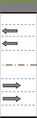
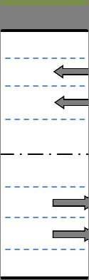
61 3.5.3 Pavement Condition The effect of pavement condition on the deflection measurement is significant. During the measurement of deflection in flexible pavement, the reading is high if that pavement has the distress like cracking or rutting. In rigid pavement, the void underneath the slab causes higher deflection value. The deflection can also be affected in this pavement by the load transfer deficiency due to lack of proper load transfer device along the joint. Deflections measured near or over a culvert show higher deflection than the expected value. The deflections of the pavement surface in cut or fill section may be deviated from exact value. 3.6 Backcalculation in Airport Pavement Evaluation This study is mainly based on the evaluation of the airport pavement strength in New Mexico. As a part of the evaluation methods, FWD data analysis is the center of focus in this literature. FWD data are collected from the airports according to the FAA guideline and thus, a number of data sets are populated for each airport pavement. The tests were carried out at various points all through the pavement and figure 3.4 shows the generalized plan of the FWD test. To cover the whole region of pavement, six test lines were selected for the evaluation. The test stations along each and every line are mentioned in the Table 3.1. At each station, three load levels of 9, 12, and 16 kips were applied. And at each load level the test is performed twice. For the analysis of the FWD data, the thickness of the individual layer is to be known. Asphalt coring and soil sampling from the pavement was the part of this project. The coring was done at every 1 ft. interval as shown in the Figure 3.5. To get a clear view of the coring strategy, 44

62 this figure shows only three coring points as an example. The FWD was done at different intervals including 2, 4, and 6 ft. that results a number of the data sets inside this coring interval. Then, for the analysis thicknesses of the layers needed to be assumed based on the adjacent coring information. The 1 ft. segment of the pavement is considered with the 5 ft. length of the pavement on either side of the coring point. The thicknesses of the surface and base course are thus collected from this pavement segment. Now, the subgrade thickness is determined by subtracting the thicknesses of the surface and base from the depth to rigid layer. The coring also gives the information about the material properties of the layer. The FWD data is then analyzed with the available information to determine the pavement layer modulus. For the analysis, the above mentioned backcalculation software are used. 3.7 Summary The above discussions in this chapter can be summarized as follows: Prior to the backcalculation process, the data relevant to the test and the pavement have to be collected. The data includes the FWD test load, pavement surface deflections due to the test load, and pavement surface temperature. From the bore log, the information about the number of layers and their individual thickness as well as the material comprising the layer have to be collected. The test data and bore log information have to be checked carefully whether there are any irregularities or potential problem involved in the data according to FAA guideline. 45

63 After having all the data with necessary checks, the layer moduli of pavement have to be backcalculated according to the steps described earlier. The backcalculated layer moduli should be reviewed for their acceptability, i.e. whether the value of the backcalculated modulus be reasonable for the individual layer, in the pavement strength evaluation. 46

64 Table 3.1: FWD test plan Test Line Distance from Centerline Test Interval 1 & 4 5 ft. c/c 2 & 5 2 ft. c/c 3 & 6 4 ft. c/c 47

65 Change in Modulus Input Seed Modulus Number of Layers Layer Thicknesses Poisson s Ratio Temperature Software Layered Elastic Analysis Method Output Measured Deflections No Compare with Field Deflections: Is the error within the specified minimum limit? Yes Modulus with least error is the final value Figure 3.1: Flow chart of the backcalculation of layer moduli 48

66 Displacement (mils) Displacement (mils) Displacement (mils) Sensor offset (inches) (a) Type Sensor offset (inches) (b) Type Sensor offset (inches) (c) Type 3 Figure 3.2: Different types of anomalies in deflection type 49

67 Load Surface Depth to Rigid Layer Base Subgrade Rigid Layer (a) Influence of the shape of deflection basin on the rigid layer depth prediction Displacement (mils) Rigid layer depth = 1/x-intercept /r (1/inches) Tangent with the initial part of the curve (b) Determination of the depth of the rigid layer Figure 3.3: Rigid layer depth determination 5

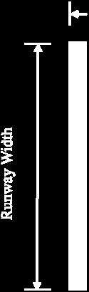
68 Figure 3.4: Generalized plan of FWD test 51

69 Coring 1 Section Length: ~1 Thickness - Surface: h 1 - Base: h 2 Coring 2 Section Length: 1 ~2 Thickness - Surface: h 1 - Base: h 2 Coring 3 Section Length: 2 ~3 Thickness - Surface: h 1 - Base: h 2 Surface Base Subgrade Figure 3.5: Layer thickness consideration for the analysis 52

70 CHAPTER 4 ACCURACY AND CONSISTENCY 4.1 Introduction Backcalculated moduli are used in important applications such as pavement design, strength evaluation, and overlay thickness design. It is important to know the accuracy and consistency of the analysis results obtained from backcalculation software. Most of backcalculation software does not produce the same layer moduli from inputs at same test point. The outputs depend on the seed or initial modulus required to run the backcalculation software. Also, the outputs vary depending on the type of the error minimization algorithm used in a specific software. There is a need for a study to select the most accurate and consistent software for the backcalculation of layer modulus to process FWD data, which is done in this chapter. 4.2 Objectives The objectives of this study are mentioned below: Examine the consistency of backcalculation software when processing FWD data of a single location using three different load levels: 9 kip, 12 kip, and 16 kip. Evaluate the accuracy of backcalculation software by comparing laboratory resilient modulus to the backcalculated modulus. In addition, compare laboratory tensile strength of asphalt concrete to field tensile strength obtained using the backcalculated moduli as inputs to a multilayer elastic analysis. Here, software accuracy is investigated based on the tensile strength of an asphalt concrete. 53

71 4.3 Study Approach In this study, asphalt cores, aggregates, and soils were collected from locations where FWD tests were conducted as a first step. Three FWD tests were conducted at each location using 9 kip, 12 kip, and 16 kip loads. The consistency of the software is evaluated through the frequency plot of the modulus backcalculated by each software. A software is considered consistent when the frequency curves of the backcalculated modulus at three loads overlap each other. To further investigate the consistency, the coefficient of variation (CV) of backcalculated moduli in response to the load increments is utilized. The higher the value of CV, the lower is the consistency. Based on this, the most consistent software is the one that shows the least CV of backcalculated moduli at the specified load levels. To verify the accuracy, software outputs are compared to the laboratory test results. Laboratory test results are considered to be the representative of the field condition. Laboratory test includes the resilient modulus and indirect tensile strength of asphalt concrete. Also, the tensile stress at the bottom of the surface AC layer is determined by KENLAYER, which is a multi-layer elastic program (Huang 24). To further investigate the accuracy, the backcalculated subgrade modulus is compared to subgrade resilient modulus obtained from California Bearing Ratio (CBR). The most suitable backcalculation software is the one that has high accuracy and consistency among three. 4.4 Data Collection and Testing Plan The FWD tests were conducted at seven runways in New Mexico. They are runway 4-22 of Double Eagle II Airport, runway 12-3 f Sierra Blanca Regional Airport, runway 2-54

72 2 and 7-25 of Raton Municipal Airport, runway 8-26 of Las Cruces International Airport, runway 8-26 of Moriarty Airport and runway 8-26 of Silver City Airport. All of these runways had surface course consists of asphalt concrete. Thirty nine bore holes were drilled in those runways to collect asphalt core, aggregates, and soil beneath. Drilling was performed at locations where FWD tests were conducted. In the FWD testing plan, each location was tested at three load levels: 9, 12, and 16 kips. At each load level, two replicate FWD tests were performed FWD Testing FWD test was performed by JILS FWD 2T. In this equipment, an impulse load was generated on the pavement surface by dropping a weight on a circular plate of 12 in. diameter from a height of 1.64 ft using a spring-mass system. The duration of the load was 2-34 milliseconds. The steel plate comes to a smooth contact with the surface of the pavement by the use of a rubber pad. Pavement deflections are measured by seven geophones resting longitudinally on the surface. Under load, the pavement surface deflects vertically downward forming a deflection basin. Seven geophones were used at different radial offset from the load. The distances of the geophones from the center of the loading plate are, 8, 12, 18, 24, 36, and 6 inches. As motioned previously, the magnitudes of the load were varied at three load levels of 9, 12, and 16 kips. For each load, two replicate tests were performed at a single test point or location. FWD test was carried out in accordance with the ASTM D

73 4.4.2 Asphalt Coring and Soil Sampling in the Field Before drilling, a preliminary drilling or coring plan was designed to cover mostly the center part of the entire runway. This was not done according to the FAA guideline, which requires coring at every 2 ft location. Because of time and funding limitations, coring performed at a spacing of 1 ft. Figure 4.1(a) shows an example of coring locations at Raton Municipal Airport in New Mexico. This airport has two runways namely, runway 7-25 and runway 2-2. Drilling was carried out at five locations in runway 7-25 and six locations in runway 2-2. Some drill locations are shown on taxiway. A detailed coring plan of runway 2-2 is shown in Figure 4.1(b). The starting point of this runway is at N latitude and W longitude. The elevation is at ft. The first drill location is 1 ft. from the start point, and the subsequent drilling or coring points are at 1 ft. spacing, alternately on both sides of the centerline. It can be seen that core or drill no. 9, 11, and 13 are located 29, 13, and 17 ft. respectively from the centerline on its left. Again, core hole or drill no. 1, 12, and 14 are located 17 ft, 27.5 ft, and 13.5 ft. from the centerline on its right. The end point is at N latitude and W longitude. The elevation is at ft. At each drill location, four coring were made to collect four asphalt samples. The soil and aggregate underneath the asphalt surface was collected. Borehole information for core location number 9 is shown in Table 4.1. A brief summary of the coring location, layer thickness, and layer properties were documented during field testing and are presented in Table 4.1. The first column shows the coring location from the start point and the distances are in ft. Samples were collected in sacks. The second column shows the identification number of sack. The third column shows the 56

74 identification number of hole. The asphalt cores, base, and subgrade materials were collected from each of these holes. At each hole, the layers were identified by A, B, C, and D. If different soils encountered, they were collected in different bags and identified with letters such as C, D, E, and F. The fifth and sixth columns show the layer information. The seventh column shows the source of the materials such as the surface, base, or subgrade. The soil type information was recorded based on field or visual identification. Table 4.2 presents the summary of the number of cores, layer type and thickness, and subgrade soil classification form laboratory testing. For example, the subgrade soils of runway 12-3 at Sierra Blanca Regional Airport and runway 2-2 at Raton Municipal Airport are clayey gravel, whereas subgrade soils of runway 7-25 at Raton Municipal Airport varies from clayey sand to gravel with sand and silt. The subgrade of the rest of the runways is silty sand. The thickness of the surface course varies from 2.25 inch to 9.75 inch, with a mean of 5.77 inch and standard deviation of 1.86 inch. The base course thickness varies from 5 inch to 15 inch, with a mean of 9.67 inch and standard deviation of 3.1 inch. 4.5 Laboratory Testing Resilient Modulus of Asphalt Concrete Asphalt cores were tested to determine the resilient modulus using an indirect tensile resilient modulus testing apparatus from Retsina Co. at the Pavement Laboratory at the University of New Mexico. Many asphalt samples were found to have thickness less than 4 inch after extraction, although the total thickness of the surface layer was more than 6 57

75 inch. It is possible that several thin layers of asphalt were laid to get to the total thickness because of compaction limitation. These thin asphalt cores are not suitable for cylindrical or axial test. Therefore, indirect tension modulus test was selected for these samples (ASTM D 4123). In indirect resilient modulus test, asphalt core sample was subjected to a repeated load of 3 lb along its diametric axis as shown in Figure 4.2(a). The thickness of the core was measured at four points which are 9º apart and the average thickness was determined. All the tests were carried out at room temperature (23.2±1ºC) and three replicate tests conducted on each sample. The repeated load and the recoverable horizontal deformation were recorded. The resilient modulus is calculated using the following formula (ASTM D 4123): where, M = resilient modulus (psi), P = repeated load (lbs), δ = total recoverable horizontal deformation (inch), t = specimen thickness (inch), and ν = Poisson s ratio. Poisson s ratio for asphalt concrete was assumed to be.35 (Huang 24). Table 4.3 shows the resilient modulus of asphalt concrete cores from seven runways. It can be seen that, the resilient modulus of runway 4-22 of Double Eagle II airport varies from 23.1 to ksi, and for runway 12-3 of Sierra Blanca Regional airport is within the range from to 27.9 ksi. The maximum value of resilient modulus is observed ksi at runway 4-22 of Double Eagle II airport and the minimum of 22.3 ksi at runway 7-25 of Raton Municipal Airport. The modulus values are mostly around 25 ksi and below 3 ksi. Generally resilient modulus of new asphalt pavements varies from 5 to 2 ksi (Tarefder et al. 27). Based on that, it can be suggested that the runway 58

76 pavements have lost their modulus values at least 5%. In other words, it can be roughly said that these runway asphalt concretes structural capacity reduced 5% or half of their design life Indirect Tensile Strength of Asphalt Concrete Indirect Tensile Strength (ITS) tests of the asphalt cores were conducted using a Humboldt device as shown in Figure 4.2(b). In this equipment, asphalt sample was loaded across its vertical diametric plane with a loading rate of 5 mm/minute (ASTM D ). Load-displacement data was collected using LabVIEW software. All the tests were carried out at room temperature (23.2±1ºC). The maximum load at failure was recorded and the ITS is calculated using the following formula: where, S = indirect tensile strength (psi), P = maximum load (lb), t = core length (inch), and D = core diameter (inch). The values of the ITS are shown in Table 4.3. For example, the ITS of AC from Runway 4-22 of Double Eagle II airport varies from 23.4 to psi and for runway 12-3 of Sierra Blanca Regional airport varies from to 36. psi. Most of the runways have shown an ITS value above 2 psi, which is a bit high, compared to the roadway pavements ITS values. ITS values are often related to the low temperature cracking of asphalt pavement (MEPDG 24). 59

77 4.6 Consistency of the Software Frequency Plot of M r As mentioned previously, consistency of software is analyzed by comparing software outputs from three sets of data varied for three load levels at a single location in the field. A frequency plot of these backcalculated moduli (M r ) of cores from 39 locations are performed at 3 load levels. If the frequency plots for these 3 load levels overlap on each other, it can be said that there is little to no variation in the backcalculated modulus due to those loads. In other words, the software is consistent. The frequency distribution includes a total of seventy eight data points (39 cores x 2 replicate tests). Figure 4.3 is plotted to examine the consistency of the software for the surface layer. From Figure 4.3(a), it is observed that the frequency distributions of the backcalculated surface modulus from MODULUS at the specified loads overlap on each other over the range 2-75 ksi. After that, the lines deviate slightly and converge at 2 ksi. The frequency distribution plots of EVERCALC, shown in Figure 4.3(b), overlap in the range of 2-45 ksi. These lines then start deviating from each other and converge again at 15 ksi. The frequency distributions of BAKFAA shown in Figure 4.3(c) do not overlap over the modulus variation. From these plots, it can be said that the MODULUS is the most consistent for the backcalculation of surface modulus. The aforementioned frequency plots are shown in Figure 4.4 and 4.5 for the base and subgrade layer, respectively. Figure 4.4(a) shows that the frequency distributions from EVERCALC start deviating from each other after 3 ksi. These lines do not overlap at any the range of modulus variation except at 175 ksi. At a base modulus value of 5 ksi, 6

78 the frequencies of 9, 12, and 16 kip load lines are 38, 31, and 33, respectively. Whereas at M r =1 ksi, the frequencies are 13, 22, and 17 units. From Figure 4.4(b), it can be seen that the frequency distributions from EVERCALC overlap at 12 and 16 kip loads for almost all the modulus variation except at M r =1 ksi. The frequency distribution of 9 kip shows the maximum deviation from those of 12 and 16 kip at M r = 5 ksi. The magnitudes of these frequencies are 13, 8 and 8, respectively. From Figure 4.4(c), it is clearly evident that the deviations in the frequency distributions of the base modulus from BAKFAA are noteworthy. The lines do not overlap over the modulus variations. Therefore, it can be said that EVERCALC is the most consistent among three for base modulus calculation. Frequency plots of subgrade are shown in Figure 4.5. It can be seen that all the software are nearly consistent except MODULUS. The large deviations in the frequency distributions from MODULUS software are observed at the modulus values of 1, 15, and 2 ksi. To that end, it can be concluded that MODULUS is not consistent software for the subgrade modulus Frequency Plot of CV of M r To further examine the consistency of backcalculation software, the coefficient of variation (CV) of the layer moduli is determined at each test point using the following formula: %

79 where, = standard deviation, and µ = mean of the backcalculated modulus using three different loads. Table 4.4 shows the CV of the backcalculated moduli obtained from three software. Due to space limitation, data of runway 8-26 of Silver City Airport is shown and discussed here. From Table 4.4, it is evident that the CV of surface modulus from MODULUS is the smallest. Both EVERCALC and BAKFAA show higher CV values at this location or data point. For base and subgrade modulus, clearly EVERCALC has the smallest CV value. However, this is only for this single data point at Silver City Airport. To get a general trend of the consistency of the analysis methods, frequency distribution of the CV for all data points is plotted as described in the following paragraph. In the frequency vs. CV plot, if the peak of the distribution leans towards the lower values of CV that indicates the majority of the data have low CV. That means that the variation in that data set is small. On the other hand, if the peak of the distribution leans towards a high value of CV, it indicates that the majority of the test data have low CV. It means that the variation is high in that data set. Therefore, the most consistent software is the one that shows the peak value of frequency at smaller CV value. But, this is not the only criterion for a software to be considered the most consistent. The shape of the frequency distribution curve must be investigated to observe the amount of deviation that an analysis shows. Surface Modulus The percentage frequency distributions of the CV of backcalculated surface modulus are plotted in Figure 4.6(a). At CV of, the frequencies of MODULUS, EVERCALC, and BAKFAA are 6, 54, and, respectively. It is observed that the frequency of EVERCALC decreases more rapidly than that of MODULUS after the peak value, 62

80 whereas BAKFAA still increases. BAKFAA shows the peak frequency 19 at a CV value of 1. It also shows the frequencies of 8 and 9 at the CV values of 3 and 5, respectively. Therefore, the backcalculated surface modulus from BAKFAA is not very consistent. MODULUS and EVERCALC analysis results are reasonably consistent though both of them show high variations with at some points. Base Modulus Figure 4.6(b) shows the percentage frequency distribution of the CV of the backcalculated base modulus from three software. The percentage frequency of MODULUS is 36 at the CV of, whereas that of the EVERCALC is 62, and BAKFAA is 18. It means that the deviation in the analysis results is lower from EVERCALC than that from MODULUS and BAKFAA. The CV value from EVERCALC converges smoothly to the zero soon after the peak value and this rate is more rapid than MODULUS. The fluctuation in CV value from BAKFAA is high. It can be said that EVERCALC is the most consistent for the backcalculation of base modulus. Subgrade Modulus Figure 4.6(c) shows the frequency distribution of the CV of the backcalculated subgrade moduli from three software as well as from AASHTO At the CV of, the frequency of EVERCALC is 31 whereas that of the other software is zero. It can be seen that the peak percentage frequencies of MODULUS, EVERCALC, BAKFAA, and AASHTO 1993 are 13, 47, 26 and 82, respectively at the CV of 5. Above the CV value of 5, the frequency values from all software decreases gradually except MODULUS software. MODULUS has attained at the peak frequency 47 at a CV value of 1. For 63

81 EVERCALC and AASHTO 1993, the shape of the curves are almost flat and parallel to the horizontal axis compared to others. It means the CV fluctuation is smaller in EVERCALC and AASHTO 1993 than that in MODULUS and BAKFAA. So, it can be said that EVERCALC and AASHTO 1993 can backcalculate the subgrade modulus more consistently than the MODULUS and BAKFAA software. 4.7 Accuracy of the Software Software accuracy will be examined based on the rule as follows: a software is accurate if it produces modulus values that match the modulus values measured in the laboratory Backcalculated vs. Measured Modulus of Asphalt Concrete Three out of four cores collected from each of the 39 drilling locations were tested for modulus in the laboratory. The average of the three core values is reported to be representative value of modulus for a single drilling location. In this section, average resilient modulus value of asphalt concrete is compared to the backcalculated FWD modulus from 9, 12, and 16 kip load FWD tests data. Based on 9 kip load The accuracy of the backcalculated modulus is examined by plotting backcalculated modulus against laboratory modulus as shown in Figure 4.7. The accuracy is indicated by a line of equality (on which backcalculated value is equal to the measured value). If the data points are close to or on the line of equality, backcalculated surface modulus is accurate. From Figures 4.7(a), 4.7(b), and 4.7(c), it can be seen that most of the data points from EVERCALC are close to the line of equality. That is, EVERCALC shows the 64

82 majority of the data fall near to the line of equality among the three software. Therefore it can said that at 9 kip load the EVERCALC software produces surface modulus that are close to the laboratory resilient modulus. Based on 12 kip load Figure 4.8(a) compares these software accuracy at 12 kip load. It can be seen that majority of data from EVERCALC backcalculation is near to the line of equality. The backcalculated surface moduli from the other MODULUS and BAKFAA software are scattered over a wide range and away from the line of equality. Therefore, it can be concluded that EVERCALC analysis results are more accurate than other software. Based on 16 kip load Figure 4.8(b) is plotted to check the accuracy of these software at 16 kip load. Again, the data points near to the line of equality are from EVERCALC software. Therefore, again at 16 kip load EVERCALC is more accurate than MODULUS and BAKFAA software Backcalculated vs. Measured Modulus of Subgrade In this section software accuracy is examined by comparing backcalculated subgrade modulus to measured modulus. As mentioned previously, resilient modulus of subgrade soil was not obtained directly by conducting laboratory testing. Soils index property testing and classification were performed in the laboratory. Modulus value was then obtained from existing relationships of soil index properties and resilient modulus of soil and it is termed as soils laboratory modulus in this paper. Several authors including Witczak et al. (1995) mentioned a number of empirical relations between resilient 65

83 modulus and subgrade CBR (Heukelom and Klomp, 1962, Heukelom and Foster, 196). Gopalakrishnan and Thompson (27) suggested that the following correlation is reasonable when applied to the subgrade modulus backcalculated from FWD measurements: where, M = subgrade resilient modulus and CBR = california bearing ratio of subgrade soil. This equation is current used in the recently developed AASHTO s mechanistic empirical pavement design guide (NCHRP 24). Again, the CBR of the soil can determined from soil index properties as follows (MEPDG 28): where, D sieve size through which 6% soils pass, P % soils finer than.75 mm size, and PI plasticity index of soil. The resilient modulus of subgrade soil is then computed using the CBR. In this study, subgrade resilient modulus for every sample is determined using the Equations (4.4) to (4.6). The laboratory subgrade modulus is then compared to the backcalculated subgrade modulus. The percent deviation of laboratory and backcalculated subgrade modulus is determined by the following mathematical relationship: %

84 where, M. = backcalculated subgrade resilient modulus, and M = laboratory subgrade resilient modulus from correlation equations. Figures 4.9(a), 4.9(b), and 4.9(c) are plotted to investigate the accuracy of the software based on the subgrade modulus due to load levels 9, 12, and 16 kips. In these figures, laboratory subgrade modulus is plotted on the horizontal axis and backcalculated modulus is plotted on the vertical axis. The line of equality goes through the points at which both the laboratory and backcalculated modulus are same. A software is considered to be the most accurate when most of the data points are on the line of equality. Figures 4.9(a), 4.9(b), and 4.9(c) show that most of the backcalculated moduli from the aforementioned software are below 4 ksi along. From Figure 4.9(a), for 9 kip load, only a few data from EVERCALC is on or near to the line of equality. So, EVERCALC is more accurate than other software for 9 kip load application. Figure 4.9(b) represents the accuracy of the software for the backcalculation of subgrade modulus using 12 kip FWD test load. Again the backcalculated moduli from EVERCALC are near to the line of equality. It means that EVERCALC is still accurate for 12 kip load data analysis. Similar trend can be observed from Figure 4.9(c). Therefore, this study concludes that EVERCALC software is the most accurate in the backcalculation of subgrade modulus. 4.8 Backcalculated vs. Measured Tensile Strength of Asphalt Concrete It is known that tensile stress develops at the bottom of the asphalt layer, particularly in thin pavements, under vertical loads. This is schematically shown in Figure 4.1. Airports, as well as roadway pavements are comprised of three layers surface, base, and 67

85 subgrade underlain by a rigid layer. Each layer can be assigned a modulus of elasticity (E n ), Poisson s ratio (υ n ), and thickness (h n ), where n is the layer number. As the FWD ball is dropped on the runway pavement surface, the bottom of the asphalt or surface layer undergoes through tension. In this study, KENLAYER, a layered elastic analysis software, is employed to determine the tensile stress at the bottom of the surface asphalt layer (Huang 24). KENLAYER program requires inputs of modulus of each layer. So as first step, backcalculation software were employed to determine the layer modulus and then they are given as inputs to KENLAYER program. As the KENLAYER inputs came from the backcaculated moduli, the tensile stress (KENLAYER output) is termed as backcalculated tensile stress in this paper. The backcalculated tensile stress is then compared to the laboratory indirect tensile stress or strength for accuracy analysis. In this study, only 9 kip load is used in KENLAYER analysis. Figure 4.11 shows the backcalculateed versus laboratory tensile strength. Figure 4.11(a) shows laboratory tensile strength in horizontal axis and backcalculated tensile stress from MODULUS software in the vertical axis. Here again a line of equality is drawn to set a reference from comparison. The accuracy of the backcalculated value to the laboratory strength value can be evaluated by how close these data points from this line. The backcalculated tensile strength is equal to the laboratory value whenever a point lies on this line of equality. Figure 4.11(b) is plotted for EVERCALC and Figure 4.11(c) for BAKFAA software. From these figures, it is observed that the tensile stress calculated for EVERCALC modulus values are close to the reference line. Therefore, from the accuracy point of view, EVERCALC is the most appropriate software among the software studied herein. 68

86 4.9 Conclusion This chapter can be concluded as follows: The consistency of FWD backcalculation software is evaluated using frequency distributions of the backcalculated moduli and CV of moduli from an identical location tested at three levels of FWD loads. For surface modulus, variation in modulus and CV of EVERCALC software are slightly higher than those of MODULUS software. The base modulus variation is the least in EVERCALC. For subgrade modulus, EVERCALC is more consistent than BAKFAA and MODULUS. Overall, the variation is highest in BAKFAA, and MODULUS ranked second. EVERCALC is the most consistent backcalculation software for determining runway pavement layer moduli. The accuracy of the backcalculated surface modulus is examined by comparing backcalculated modulus to the laboratory resilient modulus. It is shown that EVERCALC produces modulus values closer to the laboratory resilient modulus compared to MODULUS and BAKFAA software. Based on the comparison of the backcalculated tensile strength to the laboratory indirect tensile strength of the asphalt core, it is shown that EVERCALC is more appropriate than MODULUS and BAKFAA software. Based on the comparison of the backcalculated subgrade modulus to the laboratory subgrade modulus, it is evident that backcalculated subgrade modulus from EVERCALC is more close to the laboratory value than that from MODULUS and BAKFAA software. 69

87 Overall, EVERCALC has the highest accuracy and consistency compared to the MODULUS and BAKFAA software. Stress dependency of the soil and aggregate is out of scope of this study for the consistency analysis. Farther study is recommended to observe the effect of stress dependent behavior of the soil and aggregate on the consistency of the analysis by the software. 7

88 Table 4.1: Borehole information in Runway 2-2 (Raton municipal airport) Subgrade Borrow Surfacing Filler Thru Pavement Lab No. Mile Post: 1 ft. Source Location: Runway 2-2 Hole & Depth Sack No. Sample Material Type From To Number Rt. or Lt. C/L 348in. Distress N/S Hole#9 A. 8. G98 B Remarks & Material Identification (1) Transverse (2) Longitudinal (3) Alligator (4) Pothole (5) Bleeding (6) Raveling (7) Polished Aggregate (8) Reflective (9) Blade Path (1) Rutting (11) Pumping Asphalt Concrete Base Course N44 C Subgrade G61 D Subgrade N72 E Subgrade G22 F Subgrade Location measured in ft. north of Runway 2 threshold Asphalt treated Gravely gray-green sandy clay (plastic clay fraction); angular 1/2-1 1/2 lithic arkose Dark gray-green sandy clay with rust and black sandy mottles Dark sandy clay (moist, moderate ribbon) Light tan sandy clay (moist, moderate ribbon, adhesive) 71

89 Table 4.2: Thicknesses of the Layers and Subgrade Soil Classification Runway Layer No. of Cores Surface RW 4-22 Base (DE II) Subgrade SP-SM SW-SM SW-SM SP-SM SW-SM SP-SM - Surface RW 12-3 Base (SBR) Subgrade GW GW SW SW SW - - Surface RW 2-2 Base (RMA) Subgrade GP-GC GW-GC SC GP GP-GC GW-GC - Surface RW 7-25 Base (RMA) GP- Subgrade SW SC GW GM Surface RW 8-26 Base (LCIA) Subgrade SP-SM SP-SM SP-SM SP-SM Surface RW 8-26 Base (MA) Subgrade SP-SM SP-SM SM SM SM SM SM Surface RW 8-26 Base (SCA) Subgrade SP-SC SW-SC SP-SM SP SP-SM SW SM Note: Thicknesses of the layers are in inches 72

90 Table 4.3: Resilient Modulus and Indirect Tensile Strength of Asphalt Core Runway RW 4-22 (DE II) RW 12-3 (SBR) RW 2-2 (RMA) RW 7-25 (RMA) RW 8-26 (LCIA) RW 8-26 (MA) Core number Test Mean M r ITS M r ITS M r ITS M r ITS M r IDT M r ITS RW 8-26 M r (SCA) ITS Note 1: Resilient modulus is in ksi Note 2: Indirect tensile strength in psi 73

91 Table 4.4: CV of a test location (MP 6 ft.) at Runway 8-26 at Silvercity Airport Layer Surface Base Subgrade Software Load (kip) CV (%) MODULUS EVERCALC BAKFAA MODULUS EVERCALC BAKFAA MODULUS EVERCALC BAKFAA AASHTO

92 Runway 7-25 Runway 2-2 (a) Raton municipal airport End Point Width: 75 ft. Core#14 Core#13 Core#12 Core#11 Core#1 Core#9 Centerline Start Point W N S E Length: 6328 ft. (b) Coring plan of Runway 2-2 Figure 4.1: Data collection Raton Municipal Airport 75

93 Load Cell Asphalt Core Data Acquisition Device Lateral Deflection Measuring Sensor (a) Resilient modulus Load Cell Load Frame Asphalt Core (b) Indirect tensile strength Figure 4.2: Laboratory resilient modulus and Indirect tensile strength test 76

94 % Frequency kip 12 kip 16 kip % Frequency kip 12 kip 16 kip Surface modulus (ksi) Surface modulus (ksi) (a) MODULUS 6. (b) EVERCALC 5. % Frequency kip 12 kip 16 kip Surface modulus (ksi) (c) BAKFAA Figure 4.3: Frequency distribution of the surface modulus 77

95 % Frequency kip 12 kip 16 kip % Frequency kip 12 kip 16 kip Base modulus (ksi) Base modulus (ksi) (a) MODULUS 6. (b) EVERCALC 5. %Frequency kip 12 kip 16 kip Base modulus (ksi) (c) BAKFAA Figure 4.4: Frequency distribution of base modulus 78

96 % Frequency kip 12 kip 16 kip % Frequency kip 12 kip 16 kip Subgrade modulus (ksi) Subgrade modulus (ksi) (a) MODULUS 6. (b) EVERCALC 5. % Frequency kip 12 kip 16 kip % Frequency kip 12 kip 16 kip Subgrade modulus (ksi) Subgrade modulus (ksi) (c) BAKFAA (d) AASHTO 1993 Figure 4.5: Frequency distribution subgrade modulus 79

97 % frequency MODULUS EVERCALC BAKFAA 5 1 CV (%) % frequency MODULUS EVERCALC BAKFAA 5 1 CV (%) (a) Surface modulus (b) Base modulus % frequency MODULUS EVERCALC BAKFAA AASHTO 5 1 CV (%) (c) Subgrade modulus Figure 4.6: Frequency distribution of coefficient of variation of the analysis 8

98 Backcalculated modulus, ksi Backcalculated modulus, ksi Laboratory resilient modulus, ksi Laboratory resilient modulus, ksi (a) MODULUS 6. (b) EVERCALC 5. Backcalculated modulus, ksi Laboratory resilient modulus, ksi (c) BAKFAA Figure 4.7: Backcalculated surface modulus vs. Laboratory resilient modulus (9 kip load) 81

99 5 Backcalculated modulus, ksi MODULUS 25 EVERCALC 2 BAKFAA Laboratory resilient modulus, ksi (a) Based on 12 k load Backcalculated modulus, ksi MODULUS EVERCALC BAKFAA Laboratory resilient modulus, ksi (b) Based on 16 k load Figure 4.8: Backcalculated surface modulus vs. Laboratory resilient modulus 82

100 Backcalculated modulus, ksi MODULUS EVERCALC BAKFAA AASHTO Backcalculated modulus, ksi MODULUS EVERCALC BAKFAA AASHTO Laboratory modulus, ksi Laboratory modulus, ksi (a) Based on 9 k load (b) Based on 12 k load Backcalculated modulus, ksi MODULUS EVERCALC BAKFAA AASHTO 5 1 Laboratory modulus, ksi (c) Based on 16 k load Figure 4.9: Backcalculated modulus vs. Subgrade modulus for accuracy 83

101 9 lb Surface: E 1, υ 1 h 1 Base: E 2, υ 2 σ r h 2 Subgrade: E 3, υ 3 h 3 Figure 4.1: Tensile stress developed at the bottom of the surface course 84

102 Backcalculated Tensile strength,psi Backcalculated tensile strength, psi Laboratory indirect tensile strength, psi Laboratory indirect tensile strength, psi (a) MODULUS 6. (b) EVERCALC 5. Backcalculated tensile strength, psi Laboratory indirect tensile strength, psi (c) BAKFAA Figure 4.11: Backcalculated vs. Laboratory tensile strength 85

103 CHAPTER 5 FINITE ELEMENT MODELING OF FWD DEFLECTION 5.1 Introduction Finite element modeling (FEM) technique can be used for characterization of the pavement response under transient load from highway traffic, aircraft gears etc. However, most of the backcalculation software use layered elastic theory to determine pavement response, where the applied load is considered static with other assumptions. With the layered elastic theory, it is not possible to accurately predict pavement response with different geometric shape, load type, and material properties, especially, if the materials show elasto-plastic behavior. This study focuses on FEM to predict dynamic response of pavement due to impulse loading in FWD test. In the FWD test, time-deflection history is recorded at each and every sensor located at different radial offsets under the short time dynamic loading. Deflection basin is obtained from the peak displacements of those timedeflection histories. As such, it is more appropriate to perform dynamic analysis of the flexible pavement for the accurate prediction of the pavement response. This chapter covers FEM analysis on different geometries of the layered pavement structure with varying layer material properties. 5.2 Objectives The objectives of this study are: - To model the peak displacements at each sensor due to the impulse generated by a circular load on the pavement surface. In addition, to determine the time of 86

104 occurrence of the time-deflection history at each sensor and also, the relative time lag between the sensors. - FEM model output is validated by comparing the predicted time-deflection history to the field measured time-deflection history. - To determine the variation in the peak deflection with different combination of the layer moduli. - The static analysis is also performed by FEM and the output from this analysis is compared to field FWD basin. - The static analysis output is compared to that of the dynamic analysis. - The contours of vertical deflection and von Mises stress are plotted to observe their distribution over the model. The time-deflection history data are collected from the FWD test by NMDOT airfield evaluation team on runway 12-3 in Clayton Airport. The test was done with JILS FWD 2T. Only one data was used due to significant time requires for FEM study. The information about the layer thicknesses and properties are obtained from the core log of the runway. 5.3 FEM Model Description The dynamic response characterization by finite element method needs the development of a model that can be representative of the field condition. To develop a model of the multi-layered flexible pavement structure, the following steps were involved: Selection of model geometry. Assignment of layer property. 87

105 Meshing of the model, i.e. discretization of the model geometry with the appropriate elements. Imposing the boundary condition that matches with that during the field test. Application of dynamic loading criteria, i.e. determination of the amplitude pattern for the application of dynamic load during FWD test Model Geometry The geometry of the model in finite element analysis is an important factor to accurately predict the model behavior under load. From the core log information it is evident that airport pavements have mainly three different layers and they are surface, base, and subgrade, respectively. During the FWD test, the load is applied on the pavement surface through a steel plate with a radius of 6 inches. The short time loading pulse causes an instantaneous response of the pavement surface. The sensors at the different radial locations record the vertical movement of the pavement as shown in the Figure 5.1. At a certain radius, the surface deflection is assumed to be same in all the radial direction. Thus, it forms a deflection basin/influence zone. Seven sensors at different offsets measure the vertical deflections during the test. The radial distances of the sensors from the loading plate in this project are, 8, 12, 18, 24, 36, and 6 inches, respectively. The maximum deflection is recorded at the loading point and gradually, decreases with the increase in the distance. For the finite element modeling of multi layered pavement structure, different geometries are used by the researchers for the analysis. These model geometries can be either 2D plane strain, axisymmetric or 3D cube. 88

106 The two-dimensional plane strain model is used by a number of researchers to characterize the behavior of pavement (van Metzinger and McCullough 1991, and Lytton et al 1993). It requires little computation time and memory storage for the analysis. However, it can represent the actual traffic loading and the footprint of the loading is typically elliptical. It can be used represented by a two semi circles and a rectangle. The plane strain model only uses the line load (Cho 1997). The axi-symmetric model is in a geometry developed in 2D and then, revolved around with reference to a vertical axis to form a cylinder (Thompson 1982, and Nam 1994). The advantage of this model that it can solve the problem of a 3D structure with the 2D formulation using cylindrical coordinates. The main limitation of this model is that only the circular load can be applied on this model. The load assignment from the dual tire is complicated. Moreover, this model is unable to consider interface shear, though a special case of all-round radial shear can be analyzed. It can not address the pavement discontinuities or shoulder conditions. Therefore, this model can be used only for the region of the pavement far from any cracks or shoulder (Cho 1997). The 3D FEM can address different issues related to pavement, such as, multiple wheel loading, nonlinear behavior of base materials, and distresses in pavements (Kuo and Chou 24). It can correctly analyze the structural response of pavement-subgrade systems subjected to static and dynamic loads for new pavements as well as the pavement with joints, cracks, and discontinuities. The traditional 2D finite element model is not able to address these problems (Uddin et al 1995). However, it requires long time and large storage capacity, especially with material the non-linearity (Hjelmstad et al 1997). Data preparation for this type of model is more labor intensive (Cho et al 1997). 89

107 This study performs the finite element analysis using both axi-symmetric and quarter cube geometries of the flexible pavement to represent the actual field condition and loading configuration of FWD test. The details of the geometries are mentioned below: Axi-symmetric Axi-symmetric model is symmetric in all the radial directions with reference to the vertical axis. Figure 5.2 shows the axi-symmetric structure of the pavement under the FWD test. It has three layers, i.e. surface, base, and subgrade, of finite thickness individually. The thicknesses of the surface and base are 2 and 18 inches, respectively. The influence of the footing becomes insignificant for a homogenous soil if the vertical distance is considered four to ten times the width of the footing (Yamada 197, Koswara 1983, and Dunlop et al 197). The height of the pavement model is assigned 2 inches and thus, the thickness of the subgrade is limited to 182 inches that is greater than ten times diameter of the loading plate. From the field FWD test, it is generally seen that the deflection at the last sensor is too small and some distances after the last sensor it becomes zero. The reason for this small deflection at that distance is due to the vertical stress in subgrade and the stress at a large depth is negligible (Huang 24). The geometry or the domain size mainly depends upon the stress distribution in the model. Since most of the deformation takes place in subgrade, a small domain size is enough to capture the stress and thus, stress is the important factor for the domain size (Hjelmstad 1997). Considering this fact and to reduce the computation time, the radial distance of the surface and base courses is limited to 8 inches. The radial distance of the subgrade is considered 2 inches since the 9

108 deflection at farther sensor is due to stress in subgrade. A uniform pressure is applied on an area of 6 inches radius. In FWD test, sensors at different offsets from the loading point measure the vertical deflection in response to test load. Similar to the FWD test, the points with the same offsets from the loading point are assigned on the top surface of the model. The time histories of deflections from the analysis are recorded at these points. Quarter Cube The cube of the flexible pavement structure under FWD test has two axes of symmetry. Therefore, to save the time and storage capacity for the analysis, the quarter of the cube is modeled in this study for the analysis. The model is shown in the Figure 5.3. Each individual layer has the finite thickness. Similar to the axi-symmetric model the thicknesses of the surface and base of this model are 2 and 18 inches, respectively. Both of the width and height of this model are 2 inches. For this reason, to maintain the similarity in the dimensions, the length, width and breadth of the quarter cube model are 2, 2, and 2 inches, respectively. A quarter of the circle with radius of 6 inches is assigned on the top of the pavement for the application of uniform pressure to match with the FWD test load. To determine the pavement surface deflections at different sensor locations from the analysis, the points are assigned along the loading edge (Figure 5.3) according to the offsets of sensors in field test. The deflections at these points are calculated to observe the nearness of the analysis values to the field values. 91

109 5.3.2 Layer Property The model has three layers: surface, base, and subgrade. The top most layer of the pavement structure is surface course and it consists of asphalt concrete. The layer underneath the surface course is base course and it contains the compacted coarse graded gravelly soil. The bottom layer is the subgrade and it contains the natural soil. Separate material property has to be assigned for each and every individual layer since they behave in different manner in response to the impulse during the FWD test. The material properties are discussed below. Surface Course The main constituent of the surface course is asphalt concrete. Asphalt concrete is the combination of graded aggregate and asphalt binder. Thus, the whole mass has the viscoelastic property where the aggregate is responsible for elasticity and the binder is for viscosity. The effect of the visco-elasticity is pronounced at the higher temperature and at the load with slower rate. The FWD load is instantaneous and thus, the strain is recoverable. The strain will disappear just after the removal of load (Haddad 1995). Therefore, the asphalt concrete will behave as elastic material during this very short duration of loading time. Also FWD test was done at intermediate temperature of the pavement. For this reason, the surface course is assumed as linear elastic material in this analysis. Base Course In the analysis based on layered elastic theory, the base material is assumed as linear elastic. To accurately predict the pavement response, material behavior definition should 92

110 be more realistic. The granular base material can be assumed elastic up to certain limit and after that it may show plastic behavior. Modeling should consider plastic deformation beyond the elastic limit. The point at which the plastic deformation begins is known as yield point (Hibbeler 25). Once the stress due to the applied load reaches the yield point, the plastic strain path can be either linear or a curve. In finite element analysis, the stress-strain distribution has to assigned to address the strain path of a material under stress variation. The stress-strain distribution of the granular soil can be determined by performing the laboratory testing such as triaxial test. In this test, a soil sample is first subjected to an all around pressure and then, the axial stress is being increased keeping the confining stress constant (Das 1983). The increased amount of axial stress is known as deviator stress, i.e. difference between the axial and radial stress (Wood 199). The application of the deviator stress continues till the failure of the sample. The region of the stress-strain distribution before yield point is elastic and the strain is plastic after the yield point. From the FWD test data and field condition, it is evident that this test is a rapid process. Therefore, to assign the stress-strain distribution of the base course in finite element modeling, the load rate in triaxial test should be rapid. The triaxial test is out of the scope of this study. For this reason, the stress-strain distribution is collected from the study conducted by Garg nd Thompson (1997). They performed several triaxial tests with rapid load rate on different types of granular soil. In their study, they first classified the soils depending on some properties such as unit weight, friction angle. Then, they performed the triaxial tests on different groups of granular soil. The soil with known friction angle can be assumed to have the same stress-strain distribution as it observed 93

111 from the study of Garg and Thompson (1997). For this reason, this study conducted the direct shear test of the aggregate in base course to measure the shear strength as well as the angle of friction (ASTM D38-4) in the laboratory. The particle size distribution test was also measured to aid in classification of the base material. Generally, the base material from the airport does have the friction angle of 39 degree (from direct shear test in the laboratory). According to the Garg and Thompson (1997) the soil is classified as CL-5 sp. The stress-strain distribution is then obtained from the rapid shear test (triaxial test with rapid load rate). The stress-strain distribution of the granular material for the base course is mentioned in the Figure 5.4. This distribution is assigned in the analysis to integrate the real property of the base material. For the analysis, the yield point of this stress-strain distribution is considered 7 psi since the part of the curve before this yield stress can reasonably be assumed as linear elastic. The base is assumed to show plasticity whenever the stress at any point in this layer due to FWD load will exceed the deviator stress of 7 psi. The initial modulus of elasticity for the base material is assumed according to the guideline from MEPDG (28). Subgrade The subgrade contains the natural soil. Similar to the base material, the stress-strain distribution of the subgrade can also be determined from triaxial test that can be used as the material property in the finite element analysis. To perform the triaxial test of the subgrade soil was out of the scope of this study. As mentioned previously, the FWD load is instantaneous and the subgrade does not have much time to drain the pore water during 94

112 the FWD test. The consolidated undrained triaxial test data is assumed as the accurate stress-strain distribution of the subgrade for the considerations of FWD test. A number of researchers and organizations have performed triaxial tests on different types of soil. The subgrade soil in the Clayton airport was found silty clay from the soil index property determined by laboratory test. Then, for the assignment of the subgrade stress-strain distribution, the triaxial data are collected from (Slope Stability 23). Figure 5.5 shows the stress-strain distribution of the subgrade. As mentioned earlier in the case of base material, the subgrade will start showing plasticity whenever the stress at any point in this layer will reach the yield point. The yield stress in this distribution is assumed to be 1.5 T/sft (2.84 psi). And taken into consideration, the stress-strain path in the laboratory triaxial test is assigned in the analysis to address the material behavior. The dynamic analysis of the multilayered flexible pavement structure by finite element method is performed in this study using different combinations of initial layer moduli. The modulus of elasticity of different individual layers is mentioned in Table Meshing of Model Mesh assignment is an important influencing factor in the finite element modeling. The accuracy of the model is affected by the quality of the mesh. The situation is more complicated in case of dynamic analysis because the wave travel time depends on the wave velocity and the length of the mesh. Another critical situation is the meshing near the loading area as there may be a sharp change in the stress. The mesh assignment for the models is mentioned below. 95

113 Axi-symmetric The axi-symmetric model of the multi layered flexible pavement structure is meshed finely near the loading region. The region with the sensor points is also finely meshed to ensure the smooth movement of the stress wave through the medium. The region farther from the loading region is not as critical as the region near the loading region. Therefore, the mesh in that region can be coarser to perform the analysis faster. This model is of irregular geometry, i.e. the length and thickness of the surface and base course are smaller than those of the subgrade. The surface and base courses are near to the loading and sensor location whereas the subgrade is farther away from the loading area. The surface and base are meshed with smaller elements and the subgrade is meshed with coarse elements. During the meshing with different sized elements with maintaining regular geometry of the model, the mesh transition is done according to the Figure 5.6. The analysis is performed in ABAQUS/Explicit. The 4-noded quadrilateral element is used for the mesh assignment. The aspect ratio of the mesh elements were kept between 1 and 2 all through the model. Aspect ratio is defined as the ratio of the longest dimension to the shortest dimension (Logan 27). Quarter Cube The quarter cube model of the multilayered pavement structure is meshed with hexahedral or brick element and the meshing of the model is mentioned in Figure 5.7. Each individual element has eight nodes. In this analysis, the region near to the loading area is more critical than that farther away. So, the finer mesh is necessary for the loading zone whereas the mesh can be coarser near the end. The model developed for this study is 96

114 cube with identical length, breadth, and height. This geometry leads to the uniform meshing of the model though it increases the analysis time and needs more storage of the memory. The coarse mesh in the farther region is avoided due to maintain the aspect ratio between 1~2. Aspect ratio is an important factor in the analysis and the variation of the aspect ratio is responsible for the accuracy (Logan 27). The parameters of the mesh are summarized for both axi-symmetric and quarter cube in Table 5.2. It provides the information about the nodes and elements of the model during mesh assignment Boundary Condition Boundary condition is the known condition of the force and displacement, i.e. known values of the force and displacements at the nodes. The finite element analysis in ABAQUS involves two stages for the analysis. The first stage contains the initial phase of the model whenever there is no load applied on the model. The second stage contains the analysis phase and in this phase, the pavement response is analyzed with the application of the load. Therefore, the boundary condition is different in those steps. Based on the field observation of pavement structure, The assignment of boundary condition on this model is described below. Axi-symmetric There is no load on the pavement surface before and after the application of the FWD test load. The interfaces at the two adjacent layers are fully bonded (slip is not allowed). The roller supports are assigned at the vertical left end to allow the vertical movement as well as restraining the horizontal movement. The qualitative diagram of the boundary 97

115 condition of the subgrade is mentioned in the Figure 5.2. The length of surface and base course of this model is assigned 8 inches as mentioned earlier. At the right end of this 8 inches block, there is no support. There may be chance of vertical movement at this end. For this reason, the vertical movement is not restrained here. The tensile strength in the soil is negligible. The surface is only of 2 inches that is not enough to develop tensile force to cause zero deflection. The right end of the bottom block (subgrade) is restrained to move in the horizontal direction and rollers are assigned as the support. The presence of the rigid bed rock is assumed at the bottom the subgrade that leads to no deflection at the interface of the rigid/stiff layer and subgrade. For this reason, the bottom of the model is assigned with the hinge to restrain the translational movement in all directions. Quarter Cube This study performs the finite element analysis with the application of 9 kip test load. To generate this load, a uniform pressure of 79.6 psi is applied over a quarter of the circle with the radius of 6 inches. There is no additional load on the pavement surface before and after the application of the FWD load. The interface of the two adjacent layers is assumed to be fully bonded, i.e. slip between the two adjacent layers is not allowed. In response to the FWD load, the deflection becomes zero at some depth and it indicates the presence of rigid layer at this point. To address this phenomenon, the hinge supports are assigned at the bottom of the model and thus, constrains the bottom from moving along both vertical and horizontal directions. The two intersected edges with the loading point (along two axes of symmetry) are free to move in vertical direction and are restrained in the horizontal direction from adjacent material. In this model, these edges are assigned with the roller supports to ensure this behavior of the structure. There is no movement in 98

116 horizontal direction some distances after the last sensor location. For this reason, the roller supports are also assigned at the ends of the model. The boundary condition of the model is more clearly described in Figure Loading Criteria This study performs both static and dynamic analyses of the airport pavement to evaluate FWD deflection basins. The load applications in these two different types of analyses are described below. Static Load The FWD load is the function of time. In the static analysis, the load is constant with time variation. For this reason, only the peak of the load-time history is used as a static load in this study. The magnitude of the peak is 9 kips and it develops a pressure of 79.6 psi on the loading plate of 6 inches radius. Dynamic Load The purpose of this analysis is to determine the dynamic response of the pavement under FWD test. To accurately predict the pavement response, it is necessary to follow the actual amplitude pattern to apply the impulse. For this reason, the time-load history is collected from the Clayton Airport. This model is analyzed with the application of impulse with the magnitude of 9 kip. The time dependent loading pattern is assigned according to the field test. A pressure of 79.6 psi is applied on the loading area and then, this pressure is integrated with the field time-amplitude variation to match with the loadtime history under field test. The time-load history is shown in the Figure 5.8. It is 99

117 observed from the figure that the duration of the load is 25 milliseconds and the peak has attained at 1 milliseconds. The response of the multilayered flexible pavement structure (time-deflection histories of the sensors) is mentioned in Figure Finite Element Analysis The finite element analysis is performed in ABAQUS after the development of the model. Both static and dynamic conditions of the FWD test are considered in the analyses. Two different geometries axi-symmetric and quarter cube are used separately for the static and dynamic analysis. The model is analyzed for a number of layer moduli combinations as mentioned in the MEPDG according to the layer properties. The main purpose of this analysis is to determine the FWD deflection basin. The time deflection history at the specified sensor locations are recorded from the dynamic analysis. Analyzed time-deflection histories are then compared to the field time-deflection collected from FWD test. The deflection basin obtained from the field test was also compared with the analyzed peak deflections at the sensor points Static Analysis Axi-symmetric The finite element analysis of the axi-symmetric model is performed with the application of static load. The deflections of the points at different radial offset are determined to get the FWD deflection basin. The deflection basins of this model are shown in Figure 5.1(a) to (f) for different combinations of layer modulus. For the detailed discussion, the vertical deflection is determined at the layer interface. The contour of vertical deflection and von Mises stress is also plotted to observe the distribution although the model. 1

118 Quarter Cube The static analysis is performed on the quarter cube model to observe the 3D static response of the pavement under FWD test. Similar to the axi-symmetric model, the vertical deflections are determined at different distances to evaluate the FWD deflection basins. The deflection basins for different combinations of layer modulus are shown in Figure 5.11(a) to (f). From this analysis, the vertical deflection is also determined at the layer interface. To observe the distribution of the deflection and stress over the model, the contours of vertical deflection and von Mises stress are plotted Dynamic Analysis Axi-symmetric The deflection basins developed from the analysis are shown in the Figure 5.12(a) to (f). The deflections of the sensor are calculated at each sensor point and then compared to the field values. The field values are collected from the FWD peak deflection at the runway 12-3 in Clayton Airport. The analyses are carried out for different layer moduli combinations to match the calculated deflections with the field values. In each and every plot, the modulus combinations are mentioned in the layer diagram. The layer moduli combinations are mentioned in the Table 5.1. The time-deflection histories are also determined at the sensor locations. From these results, the peak deflections and their time of occurrence, the time lag between the loading time and the response at the sensor as well as between the two successive sensors are recorded. These were done to check the nearness of the analysis results to the field values. The time-deflection histories from the pre defined sensor points are mentioned in the Figure 5.13(a) to (f). 11

119 Quarter Cube The time deflection history of the points located at different distances is analyzed for different combinations of layer moduli. During the analysis, the property of each individual layer was assigned according to the material type mentioned earlier. The duration of the analysis was 1 milliseconds and this time duration was set up due to observe the variation of the deflection with time. The peak deflection was then extracted from each analyzed time-deflection history of the specific points. These peak deflections at different offsets thus form a deflection basin. The deflection basins as well as the timedeflection histories for different combinations of layer moduli are then compared to the field FWD values. The layer moduli combinations for which the analyses were performed are mentioned in the Table 5.1. The time of peak deflection occurrence at each point is one of the major concerns in this study. This time is then compared to the original time of occurrence to observe the difference. The time lag between the peak deflections at two successive sensors is also investigated. As mentioned earlier, the field FWD time deflection history is collected from the test performed in Clayton. These data are used in this study to validate the analysis results from the model. 5.5 Discussion Static Deflection Basin Axi-symmetric Figure 5.1(a) to (f) shows the FWD deflection basins for the combinations of layer modulus as mentioned in Table 5.1. The deflection basin plotted for each layer modulus 12

120 combination is compared to the deflection basin from the runway 12-3 in Clayton airport. Figure 5.1(a) to (c) shows the deflection basin for surface and base modulus of 2 and 4 ksi, respectively, whereas the subgrade modulus is 24, 17, and 8 ksi. The peak deflection is 2.88 mils as shown in Figure 5.1(a) and the deflection diminishes as the distance increases. The deflection at the last sensor is.56 mils. The peak deflection from the field deflection basin is 35 mils and the deflection at the last sensor is 2.25 mils. The difference between the field and analyzed at the first sensor is mils. Figure 5.1(b) shows the deflection basin for the surface, base, and subgrade modulus of 2, 4, and 17 ksi. The deflection at the first sensor is mils and the difference with the field deflection is mils. The deflection at the last sensor is.84 mils whereas that in the field is 2.25 mils. Figure 5.1(c) shows the deflection basin for the layer modulus combination of 2, 4, and 8 ksi. It is observed that the deflection at the first sensor is mils with the difference of 6.14 mils from the field deflection. The deflection at the last sensor is 2.3 mils that is closest to 2.25 mils from field data. The surface modulus is raised to 3 ksi for the next three analyses while the base and subgrade modulus kept constant as earlier. Figure 5.1(d) shows the deflection basin for modulus combination of 3, 4, and 24 ksi. The deflection at the first sensor is 2.57 mils and the difference from the field is mils. The deflection at the last sensor is.57 mils and that in the field is 2.25 mils. Figure 5.1(e) shows the deflection basin for the modulus combination of 3, 4, and 17 ksi. The peak deflection is mils and the difference is mils. The deflection 13

121 at the last sensor is.85 mils. Figure 5.1(f) shows the deflection basin for modulus combination of 3, 4, and 8 ksi. The peak of the deflection basin is mils with the difference of 6.67 mils from the field. The deflection at the lat sensor is 2.6 mils which is close to the field value (2.25 mils). Quarter Cube Figure 5.11(a) to (f) shows the FWD deflection basins for the quarter cube model. The combinations of layer modulus as mentioned in Table 5.1. The deflection basin plotted for each layer modulus combination is compared to the deflection basin from the runway 12-3 in Clayton airport. Figure 5.11(a) to (c) shows the deflection basin for surface and base modulus of 2 and 4 ksi, respectively, whereas the subgrade modulus is 24, 17, and 8 ksi. The peak deflection is mils as shown in Figure 5.11(a) and the deflection diminishes as the distance increases. The deflection at the last sensor is.48 mils. The peak deflection from the field deflection basin is 35 mils and the deflection at the last sensor is 2.25 mils. The difference between the field and analyzed at the first sensor is mils. Figure 5.11(b) shows the deflection basin for the surface, base, and subgrade modulus of 2, 4, and 17 ksi. The deflection at the first sensor is mils and the difference with the field deflection is mils. The deflection at the last sensor is.32 mils whereas that in the field is 2.25 mils. Figure 5.11(c) shows the deflection basin for the layer modulus combination of 2, 4, and 8 ksi. It is observed that the deflection at the first sensor is 2.75 mils with the difference of mils from the field deflection. The deflection at the last sensor is 1.13 mils that is just half of 2.25 mils from field data. 14

122 The surface modulus is raised to 3 ksi for the next three analyses while the base and subgrade modulus kept constant as earlier. Figure 5.11(d) shows the deflection basin for modulus combination of 3, 4, and 24 ksi. The deflection at the first sensor is mils and the difference from the field is mils. The deflection at the last sensor is.32 mils and that in the field is 2.25 mils. Figure 5.11(e) shows the deflection basin for the modulus combination of 3, 4, and 17 ksi. The peak deflection is mils and the difference is mils. The deflection at the last sensor is.48 mils. Figure 5.11(f) shows the deflection basin for modulus combination of 3, 4, and 8 ksi. The peak of the deflection basin is mils with the difference of mils from the field. The deflection at the lat sensor is 1.14 mils and the difference with the field value is 1.11 mils Dynamic Deflection Basin and Time History Axi-symmetric Figure 5.12(a) to (f) shows the deflection basins determined by the dynamic analysis with the finite element method. These figures show the deflections of the same model with same stress-strain distribution but with different combinations of initial modulus of elasticity at each layer. In Figure 5.12(a) to (c), the surface and the base moduli are 2 and 4 ksi, respectively. The subgrade modulus is varied and they are 24, 17, and 8 ksi. And from the analysis, it is found that the peak deflection is equal or near to 15 mils. The maximum deflection is recorded at the center point and there is a sharp drop in the deflection. From, 1 to 2 inches the decreasing rate of deflection is too low. It may due to the application of 15

123 plasticity in the stress-strain distribution in the base layer. The thickness of the surface course is 2 inches and the base is just underneath the surface. Therefore, the stress developed in the base course due to the FWD load will be of significant amount and there is a possibility of this stress to cause nonlinear strain (may show the plastic strain). The deflections get zero at 36 inches from the center point, i.e. fifth sensor. From the figures it is also evident that the peak deflection of the basin from the field is 35 mils and there is a sharp drop in the deflection values. The decreasing rate of the deflection value is getting lower at the farther sensor points and the minimum deflection is 2 mils at the outermost sensor. The deflection basins for the mentioned layer moduli combinations from the Figure 5.12(a) to (c), do not match with the field values. The analyses were repeated for the modified layer moduli combinations with surface modulus of 3 ksi. Here, also the values of subgrade modulus are 24, 17, and 8 ksi while the surface and base modulus are kept constant at the values of 3 and 4 ksi, respectively. Figure 5.12(d) to (f) show the deflection basins analyzed for these new combinations. The duration of the analyses was increased to 1 milliseconds. There is a possibility of the stress wave with low velocity that may increase the travel time and with the analysis duration of 6 milliseconds the deflection at some sensors may be zero due to the delay in wave propagation. For this reason, the duration of the analysis is increased to capture the waves at the sensors. From the Figures 5.12(d) to (f), it is observed that there is no significant influence of the surface modulus variation on the deflection. The increase in analysis time, determined the non zero deflections at the farther sensors. In the previous analyses as mentioned in the Figure 5.12(a) to (c), the deflection is zero at the fifth sensor. Due to the increase in analysis time, the stress wave has more travel time 16

124 than that of the previous analyses to reach the farthest sensor and thus, the non zero deflection is recorded at that point. The time-deflection histories of the sensors at different radial offsets are determined to perform the tasks as mentioned in the objectives. The Figures 5.13(a) to (f) show the time-deflection histories for different combinations of layer moduli. The first three analyses were performed with the duration of 6 milli seconds. In these combinations the subgrade modulus were 24, 17, and 8 ksi while keeping the surface and base modulus constant at the values of 2 and 4 ksi, respectively. From the Figure 5.13(a), it is seen that the peak deflection at the first sensor occurs at 22.5 milli seconds and those of the second, third, fourth and fifth sensor occur at 33.6, 43.2, 56.7, and 6 milli seconds. The sixth and seventh sensors show the zero deflection. Here, in the analyses, it is observed that there is a significant amount of time lag of the peak deflection occurrence between the sensors. In the field test, the responses of the sensors were instantaneous and simultaneous. The analysis results give the indication of the larger travel time, i.e. low velocity, of the stress wave through the model. The other observation is that the deflections at the sixth and seventh sensors are recorded zero. The same incidents are observed in the Figures 5.13(b) and (c). In Figure 5.13(b), the peak deflections are recorded 22.2, 33, 44.1, 59.4, and 6 milli seconds at the first, second, third, fourth, and fifth sensor, respectively. Here, the sixth and seventh sensor points also determine the peak deflection of zero. The time of occurrence of peak deflections are recorded 22.5, 33.6, 45.3, and 6 milli seconds at first, second, third, and fourth sensor as shown in the Figure 5.13(c). Still, some sensors farther 17

125 from the loading point show the zero vertical deflection that is undesirable. This incident may be due to the large propagation time of wave through the model. For this reason, the analysis time is increased to 1 milli seconds for the next three analyses. The surface modulus is increased to 3 ksi while keeping the base modulus at 4 ksi. The subgrade modulus variation is the same as followed in the previous analyses. Figures 5.13(d) to (f) show the time-deflection histories for the new combinations of layer moduli and analysis duration. There is no significant change in the peak deflection at the first sensor as it was determined before. In the previous analyses, it was observed that the peak deflection at the fifth and the farther sensor is zero. Due to the increase in the analysis time, the time-deflection histories at the farther sensors are recorded for larger time duration. As a result, the fifth and sixth sensors have extracted the larger peak deflections. The time-deflection histories for surface, base, and subgrade modulus of 3, 4, and 24 ksi, respectively, are plotted in Figure 5.13(d). The time of occurrence of the peak deflections at the seven sensors are 22, 31.5, 44.5, 62.5, 79.5, and 1 milli seconds. The peak deflections at the last two sensors are determined at the same time, i.e. 1 milli seconds. The time lag between the successive sensors is still large but in the field FWD test, it was simultaneous. In Figures 5.13(e) and (f), the non-zero vertical deflections are recorded at the fifth sensor and so on. The time lags in these analyses are still large. Quarter Cube The dynamic analysis in finite element method was performed for the aforementioned layer moduli combinations though the stress-strain distribution for each individual layer 18

126 is still same. The deflection basins obtained from the 3D dynamic analysis are mentioned in Figure 5.14(a) through (f). In Figures 5.14(a) to (c), the deflection basins are mentioned for the surface and base modulus of 2, and 4 ksi, respectively, while changing the subgrade modulus 24, 17, and 8 ksi, respectively. The peak deflection at the first sensor is about 1 mils in Figure 5.14(a) and it gradually decreases to zero at the last sensor. The peak deflection is 35 mils in Clayton FWD deflection basin and it is three times higher than analyzed peak deflection. The subgrade modulus is 17 ksi in Figure 5.14(b) and the peak deflection is less than 1 mils that give the indication that the change in subgrade modulus does not have the pronounced effect on the peak deflection value. The deflection basin for this modulus combination does not also match with field values. The subgrade modulus is 8 ksi in Figure 5.14(c) and the peak deflection is 1 mils. The deflection reached zero magnitude at the sixth sensor (distance: 36 inches). However, the deflection basin for this combination of layer moduli does not match with field values. To observe the farther effect of modulus variation on the analysis results, the surface modulus was assigned 3 ksi while keeping the base and subgrade modulus same as before. Figure 5.14(d) to (f) shows the deflection basin with surface and base modulus of 3 and 4 ksi, respectively, whereas the subgrade modulus is 24, 17, and 8 ksi, respectively. The peak deflection is about 1 mils in Figure 5.14(a) that is much smaller than the field value. The deflection at the seventh sensor (distance: 6 inches) is zero but in the field FWD data, the deflection is non zero. So, change in surface modulus does not have significant effect in the analysis of this model. In Figure 5.14(e) and (f), the surface and base modulus are the same whereas the subgrade modulus is 17 and 8 ksi. And 19

127 variation in the subgrade modulus does not affect the deflections. This model with the mentioned combinations of layer moduli is very stiff since the deflections at the points are much smaller than the field deflections. The time-deflection histories at different sensor points are analyzed and mentioned in the Figure 5.15(a) through (f). The time-deflection history in Figure 5.15(a) is analyzed for the surface, base, and subgrade modulus of 2, 4, and 24 ksi, respectively. The peak deflection at the first sensor point occurs at 2 milli second and it is 9.87 mils. The peak value at the second sensor is observed 3.82 mils at 3 milli second and the time lag is about 1 milli second. The peak values of the time-deflection histories at the third, fourth, fifth, and sixth sensor are 2.29, 1.68, 1.26, and.64 mils, respectively. The peak at the last sensor is.66 mils. It is clearly evident from the Figure 5.15(a) that the time lag between the peak deflection values at the two adjacent sensors are significantly large whereas the peak deflections from the field FWD data are with negligible time lag as mentioned in Figure 5.9. Figure 5.15(b) shows the time-deflection histories for the modulus combination of 2, 4, and 17 ksi, respectively. The peak deflection of the first sensor is 8.26 mils and it has attained at 2 milli second. After some time lagging, the peak of the second sensor (3.58 mils) has attained at 25 milli second and the time lag of 5 milli second is a significant amount whereas the time lag in field data is nearly negligible. The peak deflections of the time-deflection histories at third, fourth, fifth, and sixth are 2.19, 1.9, 1.36, and.51 mils, respectively, and they show the time lag larger than that in field FWD data. The peak (.57 mils) at the last sensor has occurred at 94 milli second and it shows greater time lag than the field test. 11

128 The time-deflection histories of the sensors for the surface, base, and subgrade modulus of 2, 4, and 8 ksi, respectively, are mentioned in Figure 5.15(c). At 19 milli second, the peak deflection of the first sensor is 9.84 mils. And at 32 milli second, the peak is found 3.78 mils at the second sensor point. So, the time lag is 13 milli second and it is very high. The peak deflections of the third, fourth, fifth, and sixth sensors are 2.24, 1.62, 1.18, and.46 mils, respectively. These peak values occur at 47, 6, 71, and 1 milli second. The deflection at the last sensor is almost zero. The figure shows the response is not instantaneous and the times lag between the peak deflections of the adjacent sensors are larger than that from the field value. In the next three analyses, the surface modulus was increased to 3 ksi while keeping the base and subgrade moduli same as before. Figure 5.15(d) to (f) shows the timedeflection histories for surface and base modulus of 3, and 4 ksi, respectively. And the subgrade moduli are 4, 24, and 17 ksi. In Figure 5.15(d), the peak deflection at the first sensor is found 9.46 mils at 19 milli second and that at the second sensor is found 3.83 mils at 31 milli second. The time lag is 12 milli second between the first and second sensor. The peak deflections of the time-deflection histories at the third, fourth, fifth, and sixth sensors are 2.27, 1.47, 1.198, and.65 mils, respectively. And the time of occurrence of these peak values are 43, 6, 71, and 1 milli second, respectively. Still, the time lag is so high. The time-deflection histories for the moduli combination of 3, 4, and 17 ksi are plotted in Figure 5.15(e). The peak deflection of the time history in the first sensor is found 9.47 mils at 2 milli second and in the second sensor, it is found 3.82 mils at 31 milli second. The resulting time lag is 11 milli second. The peak deflections of the time- 111

129 deflection data for the third, fourth, fifth, and sixth sensors are 2.245, 1.47, 1.17, and.59 mils, respectively. And their times of occurrence are 43, 6, 72, and 1 milli second. The deflection at the last sensor is near to zero. Here, it is observed that the time lag is much higher than the time lag in field data. Figure 5.15(f) shows the time-deflection histories of the sensor points for the surface, base, and subgrade modulus of 3, 4, and 8 ksi, respectively. From this analysis, the peak deflections of the time histories at the first sensor and second sensor are 9.47, and 3.77 mils, respectively. The time-deflection histories have attained their peak values at 2 and 31 milli second, respectively. The resulting time lag between the first and second sensor is 11 milli second. The peak deflections of the time-deflection histories in other sensor are 2.14, 1.47, 1.11, and.46 mils, respectively. The time of occurrences of these peak values are 42, 61, 73, and 1 milli second. The time lags are still higher than the field data and for different combinations of layer moduli these do not vary significantly. The peak values of the time-deflection analysis results are much smaller than the FWD data from Clayton airfield pavement Deflection at Layer The vertical deflection is determined at the surface, surface-base interface, and basesubgrade interface to compare the static and dynamic analysis results. These deflections are mentioned in Table 5.3. The deflections are determined using different combinations of layer modulus for both of the geometries. Table 5.3 includes the deflections at the surface, base, and subgrade. Column six in this table shows the total deflection and the next three columns show the deflection for the surface, base, and subgrade, respectively. 112

130 It is observed that for every layer modulus combination, the static deflection is greater than the dynamic deflection for both of the models. Effect of change of modulus is more pronounced in static analysis than that in dynamic analysis. From Table 5.3, it is evident that the decrease in layer modulus causes the increase in the vertical deflection whereas the dynamic analysis is not affected significantly with the modulus variation Contour of Vertical Deflection Axi-symmetric The contours are plotted for both static and dynamic analyses cases to observe the distribution of the vertical deflection over axi-symmetric model. Two different modulus combinations are selected for these contour plots. The first combination is 2, 4, and 8 ksi and the second combination is 3, 4, and 24 ksi as the surface, base, and subgrade modulus, respectively. Figure 5.16 shows the contours of vertical deflection on axi-symmetric model for both static and dynamic analysis. Figure 5.16(a) shows the contour of static analysis whereas Figure 5.16(b) is based on dynamic analysis. These contours are plotted for the modulus combination of 2, 4, and 8 ksi. The legend at the left represents the deflection values depending upon the color variation. The blue color in the legend shows the maximum vertical downward deflection whereas the red shows the upward deflection. The color variation from blue to red represents the vertical downward deflection decreases and approaches to the upward vertical deflection. From the contour plots of two different cases, it is observed that the maximum deflection is at the corner of the model where the 113

131 load is applied. The maximum deflection for static analysis is greater than the dynamic deflection. The contours of vertical deflection are again plotted for the modulus combination of 3, 4, and 24 ksi. Figure 5.17 shows the contour plots for this modulus combination. In both of the cases the peak is observed at the corner as before. From these plots, the maximum deflection is observed in the same corner region of the model. From the contour plots, it is observed that the deflections from static analysis are greater than that from dynamic analysis. For the dynamic analysis, the deflection is higher and concentrated near to the loading point. In dynamic analysis, the peaks at different sensors were recorded at different times due to the wave stress propagation through the model. For this reason, the peak values at the sensors, except the first sensor, are not visible in this contour. On the other hand, the static analysis shows the peak deflections at every sensor in the same contour since the load in static analysis is constant with the time variation and the pavement response to the load is simultaneous. The contours of the vertical deflection for the other modulus combinations are shown in the Appendix. Quarter Cube Figure 5.18 shows the contours of vertical deflection for quarter cube considering both static and dynamic analyses cases. The modulus combination of 2, 4, and 8 ksi is considered for these contour plots. The maximum deflection is observed at the corner of the model. And the static deflection is greater than the dynamic deflection. And due to 114

132 time lag, the points other than the top corner of the model do not show the peak deflection at the same time during dynamic analysis. Figure 5.19 shows the contours for the modulus combination of 3, 4, and 24 ksi. The static deflection is also greater than the dynamic deflection. For static analysis, the contour shows the maximum deflection at every sensor points since the pavement response has been taken place simultaneously. The contour from dynamic analysis shows the peak deflections concentrated at the corner and the deflections at other points are very small due to the time lag Contour of Stress Axi-symmetric To observe the stress distribution over the axi-symmetric model, the contours are plotted based on von Mises stress. Both of the static and dynamic analyses are considered for the contour plots. Figure 5.2(a) shows the contours of von Mises stress for static analsysis and Figure 5.2(b) shows that for dynamic analysis. The modulus combination of 2, 4, and 8 ksi is considered for this analysis. The legend on the left shows that the red represents the maximum stress and the blue represents the minimum stress. The color variation from red to blue indicates the stress variation in descending order. The maximum stress for static analysis is 51.5 psi and that of the dynamic analysis is psi. Figure 5.21 shows the contours of von Mises stress for 3, 4, and 24 ksi. From the contours, the maximum of von Mises stress is determined psi for static analysis and for dynamic analysis. 115

133 Quarter Cube Figure 5.22 shows the contours of von Mises stress for quarter cube model. These contours are plotted for both static and dynamic analysis. The modulus combination of 2, 4, and 8 ksi is assumed for the analysis. The maximum for the static analysis is observed psi and that for the dynamic analysis is observed psi. Figure 5.23 shows the contours for the modulus combination of 3, 4, and 24 ksi. The maximum stress is observed 44.3 psi for static analysis and that for the dynamic analysiss is observed 44.5 psi. 5.6 Comparing Static vs. Dynamic Analysis Figure 5.24 shows the comparison of the static and dynamic analysis for axi-symmetric model. For the static analysis, six different combinations of layer modulus are considered as mentioned earlier. The static and dynamic analyses are compared based on the FWD deflection basin. The nearness of both static and dynamic deflection is also compared to the field FWD deflection from runway 12-3 in Clayton airport. For axi-symmetric model, it is observed that the static deflection is greater than the dynamic deflection and it is closer to the field deflection. Therefore, the static analysis gives better results than the dynamic analysis for ax-symmetric model. Figure 5.25 shows the comparison of the static and dynamic analysis for quarter cube model. The static analysis gives greater deflection than dynamic analysis and it is closer to the field deflection. It is evident that the static analysis results are better than dynamic analysis for the prediction of field FWD deflection basin. 116

134 5.7 Conclusions The above discussions lead to the following conclusions: For the same combination of layer moduli, the axi-symmetric and quarter cube geometries yield different analysis results. The axi-symmetric model shows higher deflections than that from quarter cube model. The peak deflections from the axi-symmetric model are closer to the field FWD data for the mentioned moduli combinations. From the field FWD data, it is observed that the response of the flexible pavement under the impulse is instantaneous and the time lags between the successive sensors are very small. In this study, the analyses show the significant amount of time lag between the two successive points and also the time of occurrence of the higher than that of the field data in both of the two different geometries. For the variation of the combinations of the layer moduli, the surface modulus is varied from 2 to 3 ksi and the subgrade modulus is varied from 17 to 4 ksi. The base modulus is kept constant. The analysis results have shown that these combinations does not affect significantly. For the mentioned moduli combinations, the peak deflections have not match with the field values. The moduli combination with lower surface and base modulus may give the deflection closer to the field data. The analysis results from the static analysis are closer to the field FWD test data. The deflection from this analysis is greater than the dynamic analysis. 117

135 Table 5.1: Modulus of elasticity of flexible pavement layer Material Type Modulus of Elasticity (ksi) Surface Base Subgrade Surface Base Subgrade HMA A-1-a A-4 (Silt) A-6 (Clay) A-7-6 (Clay) HMA A-1-a A-4 (Silt) A-6 (Clay) A-7-6 (Clay)

136 Table 5.2: Parameters of the finite element model FEM parameter Axi-symmetric Quarter cube Number of nodes 4,44 46,274 Element type CAX4R C3D8R Number of elements 4,561 49,

137 Table 5.3: Vertical deflection at the layer interface Geometry Axisymmtric Quarter cube Modulus of Elasticity (ksi) Deflection (mils) Type Surface Base Subgrade Total δ1 δ2 δ Static Dynamic Static Dynamic Static Dynamic Static Dynamic Static Dynamic Static Dynamic Static Dynamic Static Dynamic Static Dynamic Static Dynamic Static Dynamic Static Dynamic

138 Load Influence zone Geophones Surface Base Subgrade Figure 5.1: The zone of influence during FWD test 121

139 Load Surface: h 1, E 1, υ 1, ρ 1 Sensor indicator Roller Supports Base: h 2, E 2, υ 2, ρ 2 Subgrade: h 3, E 3, υ 3, ρ 3 Roller Supports Z R Hinge Supports Figure 5.2: Qualitative diagram of the Axi-symmetric model of flexible pavement 122

140 FWD test load over the one quarter of the circular loading area Sensor indicator Y X Z (a) Surface Base Surface Base Subgrade Subgrade Y Y Z X (b) Figure 5.3: Qualitative diagram of the Quarter cube model of flexible pavement 123

141 1 9 8 Deviator stress (psi) Axial strain (%) Figure 5.4: Stress-strain distribution of the granular soil in base course (Garg and Thompson, 1997) 124

142 2.5 2 Deviator stress (T/sft) Axial strain (%) Figure 5.5: Stress-strain distribution of subgrade soil from triaxial test (Slope stability 23) 125

143 Figure 5.6: Mesh refinement of the axi-symmetric model 126

144 Figure 5.7: Mesh refinement of the quarter cube model 127

145 1 Load (kips) Time (milliseconds) Figure 5.8: Amplitude pattern of the impulse in the FWD test 128

146 Displacements (mils) D1 D2 D3 D4 D5 D6 D7 Time (milli second) Figure 5.9: Time-deflection histories of the sensors 129

147 Displacement (mils) Sensor offse t (inches) 2 4 FEA Clayton 6 (a) Displacement (mils) Sensor offse t (inches) 2 4 FEA Clayton 6 (b) Displacement (mils) Sensor offse t (inches) 2 4 FEA Clayton 6 (c) Figure 5.1: Deflection basins analyzed for different layer moduli combinations (axi-symmetric static analysis) 13

148 Displacement (mils) Sensor offse t (inches) 2 4 FEA Clayton 6 (d) Displacement (mils) Sensor offse t (inches) 2 4 FEA Clayton 6 (e) Displacement (mils) Sensor offse t (inches) 2 4 FEA Clayton 6 (f) Figure 5.1: Deflection basins analyzed for different layer moduli combinations (axi-symmetric static analysis) 131

149 Displacement (mils) Sensor offse t (inches) 2 4 FEA Clayton 6 (a) Displacement (mils) Sensor offse t (inches) 2 4 FEA clayton 6 (b) Displacement (mils) Sensor offse t (inches) 2 4 FEA Clayton 6 (c) Figure 5.11: Deflection basins analyzed for different layer moduli combinations (quarter cube static analysis) 132

150 Displacement (mils) Sensor offse t (inches) 2 4 FEA Clayton 6 (d) Displacement (mils) Sensor offse t (inches) 2 4 FEA Clayton 6 (e) Displacement (mils) Sensor offse t (inches) 2 4 FEA clayton 6 (f) Figure 5.11: Deflection basins analyzed for different layer moduli combinations (quarter cube static analysis) 133

151 Displacements (mils) Sensor offset (inches) 2 4 FEA CLAYTON 6 (a) Displacements (mils) Sensor offset (inches) 2 4 FEA Clayton 6 (b) Displacements (mils) Sensor offset (inches) 2 4 FEA Clayton 6 (c) Figure 5.12: Deflection basins analyzed for different layer moduli combinations (axi-symmetric dynamic analysis) 134

152 Displacements (mils) Sensor offset (inches) 2 4 FEA Clayton 6 (d) Displacements (mils) Sensor offset (inches) 2 4 FEA Clayton 6 (e) Displacements (mils) Sensor offset (inches) 2 4 FEA Clayton 6 (f) Figure 5.12: Deflection basins analyzed for different layer moduli combinations (axi-symmetric dynamic analysis) 135

153 5 Displacements (mils) Time (milli seconds) (a) E 1 : 2, E 2 : 4, E 3 : 24 ksi D1 D2 D3 D4 D5 D6 D7 5 Displacement (mils) Time (milli seconds) D1 D2 D3 D4 D5 D6 D7 (b) E 1 : 2, E 2 : 4, and E 3 : 17 ksi 5 Displacement (mils) Time (milli seconds) D1 D2 D3 D4 D5 D6 D7 (c) E 1 : 2, E 2 : 4, and E 3 :8 ksi Figure 5.13: Time-deflection histories at the sensors for layer moduli combinations (axisymmetric dynamic analysis) 136

154 5 Displacements (mils) D1 D2 D3 D4 D5 D6 D7 Time (milli seconds) (d) E 1 : 3, E 2 : 4, and E 3 : 24 ksi 5 Displacements (mils) D1 D2 D3 D4 D5 D6 D7 Time (milli seconds) (e) E 1 : 3, E 2 : 4, and E 3 : 17ksi 5 Displacements (mils) D1 D2 D3 D4 D5 D6 D7 Time (milli seconds) (f) E 1 : 3, E 2 : 4, and E 3 : 8 ksi Figure 5.13: Time-deflection histories at the sensors for layer moduli combinations (axisymmetric dynamic analysis) 137

155 Displacements (mils) Sensor offset (inches) 2 4 FEA Clayton 6 (a) Displacements (mils) Sensor offset (inches) 2 4 FEA Clayton 6 (b) Displacements (mils) Sensor offset (inches) 2 4 FEA Clayton 6 (c) Figure 5.14: Deflection basins analyzed for different layer moduli combinations (quarter cube dynamic analysis) 138

156 Displacements (mils) Sensor offset (inches) 2 4 FEA Clayton 6 (d) Displacements (mils) Sensor offset (inches) 2 4 FEA Clayton 6 (e) Displacements (mils) Sensor offset (inches) 2 4 FEA Clayton 6 (f) Figure 5.14: Deflection basins analyzed for different layer moduli combinations (quarter cube dynamic analysis) 139

157 2 Displacement (mils) D1 D2 D3 D4 D5 D6 D7 Time (milli seconds) (a) E 1 : 2, E 2 : 4, and E 3 : 24 ksi Displacement (mils) D1 D2 D3 D4 D5 D6 D7 Time (milli seconds) (b) E 1 : 2, E 2 : 4, and E 3 : 17 ksi Displacement (mils) Time (milli seconds) D1 D2 D3 D4 D5 D6 D7 (c) E 1 : 2, E 2 : 4, and E 3 : 8 ksi Figure 5.15: Time-deflection histories at the sensors for layer moduli combinations (quarter cube dynamic analysis) 14

158 Displacement (mils) D1 D2 D3 D4 D5 D6 D7 Time (milli seconds) (d) E 1 : 3, E 2 : 4, and E 3 : 24 ksi Displacement (mils) D1 D2 D3 D4 D5 D6 D7 Time (milliseconds) (e) E 1 : 3, E 2 : 4, and E 3 : 17 ksi Displacement (mils) D1 D2 D3 D4 D5 D6 D7 Time (milli seconds) (f) E 1 : 3, E 2 : 4, and E 3 : 8 ksi Figure 5.15: Time-deflection histories at the sensors for layer moduli combinations (quarter cube dynamic analysis) 141

159 (a) Static analysis (b) Dynamic analysis Figure 5.16: Contour of vertical deflection (2, 4, and 8 ksi) 142

160 (a) Static analysis (b) Dynamic analysis Figure 5.17: Contour of vertical deflection (3, 4, and 24 ksi) 143

161 (a) Static analysis (b) Dynamic analysis Figure 5.18: Contour of vertical deflection (2, 4, and 8 ksi) 144

162 (a) Static analysis (b) Dynamic analysis Figure 5.19: Contour of vertical deflection (3, 4, and 24 ksi) 145

163 (a) Static analysis (b) Dynamic analysis Figure 5.2: Contour of von Mises stress (2, 4, and 8 ksi) 146

164 (a) Static analysis (b) Dynamic analysis Figure 5.21: Contour of von Mises stress (3, 4, and 24 ksi) 147

165 (a) Static analysis (b) Dynamic analysis Figure 5.22: Contour of von Mises stress (2, 4, and 8 ksi) 148

166 (a) Static analysis (b) Dynamic analysis Figure 5.23: Contour of von Mises stress (3, 4, and 24 ksi) 149

167 Displacements (mils) Displacements (mils) Displacements (mils) Sensor offset (inches) FEM_dynamic CLAYTON FEM_static (a) Sensor offset (inches) FEM_dynamic Clayton FEM_static (b) Sensor offset (inches) FEM_dynamic Clayton FEM_static (c) Figure 5.24: Comparison of FWD deflection basins (axi-symmetric) 15

168 Displacements (mils) Sensor offset (inches) 2 4 FEM_dynamic Clayton FEM_static 6 (d) Displacements (mils) Sensor offset (inches) 2 4 FEM_dynamic Clayton FEM_static 6 (e) Displacements (mils) Sensor offset (inches) FEM_dynamic Clayton FEM_static (f) Figure 5.24: Comparison of FWD deflection basins (axi-symmetric) 151

169 Displacements (mils) Sensor offset (inches) FEM_dynamic Clayton FEM_static (a) Displacements (mils) Sensor offset (inches) 2 4 FEM dynamic Clayton FEM static 6 (b) Displacements (mils) Sensor offset (inches) FEM static Clayton FEM dynamic (c) Figure 5.25: Comparison of FWD deflection basins (quarter cube) 152

170 Displacements (mils) Sensor offset (inches) FEM static Clayton FEM dynamic (d) Displacements (mils) Sensor offset (inches) FEM_dynamic Clayton FEM_static (e) Displacements (mils) Sensor offset (inches) FEM dynamic Clayton FEM static -4 (f) Figure 5.25: Comparison of FWD deflection basins (quarter cube) 153

171 CHAPTER 6 CONCLUSIONS This study evaluates most widely used FWD software based on accuracy and consistency to back-calculate the modulus of elasticity of the airport pavements in New Mexico. These software are BAKFAA, MODULUS 6. and EVERCALC. The purpose was to find software that can back calculate the pavement layer moduli most accurately and consistently from the FWD test data. To check the accuracy, the back calculated moduli of the surface course from the aforementioned software are compared to the resilient modulus of the asphalt concrete from laboratory testing. The indirect tensile strength test of asphalt concrete was also performed and then, the tensile stress at the bottom (determined by KENLAYER, a multi layered elastic analysis software) is compared to the laboratory indirect tensile strength of asphalt concrete to investigate the accuracy. For the further investigation of the accuracy, the back calculated subgrade modulus is compared to the field modulus determined from CBR values using the CBR-modulus empirical relationship. During the field FWD test, each and every point on the airfield was tested under three different loads and they are 9, 12, and 16 kips. To check the consistency of the analysis results from the software, the coefficient of variation (CV) of the back calculated layer moduli at these test loads is determined at every test station. The frequency distribution of the CV is then plotted to find the software that gives least variation in analysis results. For this study, FWD data were collected from seven different runways and they are Runway 4-22 of Double Eagle II, 154

172 Runway 12-3 of Sierra Blanca Regional, Runway 2-2 and 7-25 of Raton Municipal, Runway 8-26 of Las Cruces, Runway 8-26 of Moriarty, Runway 8-26 of Silver city airport. The asphalt cores and soil samples are also collected from these runways. The aforementioned software are based on the multi-layered elastic theory and for this reason, during analysis the pavement layers are assumed as linear elastic. But in reality, pavement response can not always be elastic. Therefore, for the better prediction of the pavement characteristics under FWD test, the dynamic analysis of the multi layered flexible pavement was performed by finite element method. The stress-strain distribution of the layer material was assigned as the layer properties of the FEM model. FEM analysis includes two different geometries. The first one is axi-symmetric and the second one is quarter cube model. The pavement response is analyzed in response to the impulse loading. To apply the impulse on the model, the time-load history data is used from FWD test from Clayton airport. The predicted time-deflection histories are then compared to the field response in terms of the peak deflection, the time of occurrence of the peak values, and their time lag. Based on the studies mentioned above the conclusions can be summarized as follows: The consistency of FWD backcalculation software is evaluated using frequency distributions of the backcalculated moduli and CV of moduli from an identical location tested at three levels of FWD loads. For surface modulus, variation in modulus and CV of EVERCALC software are slightly higher than those of MODULUS software. The base modulus variation is the least in EVERCALC. For subgrade modulus, EVERCALC is more consistent than BAKFAA and 155

173 MODULUS. Overall, the variation is highest in BAKFAA, and MODULUS ranked second. EVERCALC is the most consistent backcalculation software for determining runway pavement layer moduli. The accuracy of the backcalculated surface modulus is examined by comparing backcalculated modulus to the laboratory resilient modulus. It is shown that EVERCALC produces modulus values closer to the laboratory resilient modulus compared to MODULUS and BAKFAA software. The backcalculated tensile strength is compared to the laboratory indirect tensile strength of the asphalt core and it is observed that EVERCALC is more appropriate than MODULUS and BAKFAA software. The comparison of the backcalculated subgrade modulus to the laboratory subgrade modulus has shown that backcalculated subgrade modulus from EVERCALC is more close to the laboratory value than that from MODULUS and BAKFAA software. For the same combination of layer moduli, the axi-symmetric and quarter cube geometries yield different analysis results. The axi-symmetric model shows higher deflections than that from quarter cube model. The peak deflections from the axi-symmetric model are closer to the field FWD data for the mentioned moduli combinations. From the field FWD data, it is observed that the response of the flexible pavement under the impulse is instantaneous and the time lags between the successive sensors are very small. In this study, the analyses show the significant amount of time lag between the two successive points and also the time of occurrence of the higher than that of the field data in both of the two different geometries. 156

174 For the variation of the combinations of the layer moduli, the surface modulus is varied from 2 to 3 ksi and the subgrade modulus is varied from 17 to 4 ksi. The base modulus is kept constant. The analysis results have shown that these combinations does not affect significantly. The static deflection is greater than the dynamic deflection and closer to the field FWD deflection basin. The deflection in static analysis is more sensitive to the layer modulus variation than the dynamic analysis. The following points can be recommended for the future studies: The surface course in the finite element modeling was assumed linear elastic in this study. The non linear stress-strain distribution may be more appropriate to address the accurate behavior of the asphalt concrete. The models developed in this study, is analyzed for only one test point on the runway 12-3 of Clayton airport. More data points can be used for rigorous validation of the model. Also more combination of material properties can be tried in FEM analysis. The laboratory testing can be conducted on soil and aggregate to determine the actual modulus of elasticity of subgrade and base layer as well as to obtain the proper stress-strain distribution of the layer material that can be used for the finite element modeling. 157

175 REFERENCES Ameri, M., Yavari, N. and Scullion, T. (29). Comparison of Static and Dynamic Backcalculation of Flexible Pavement Layers Moduli, using four softwares. Asian Journal of Applied Sciences, Vol. 2, No. 3, pp American Association of State Highway and Transportation Officials. (1993). AASHTO Guide for Design of Pavement Structures: Rehabilitation Method with Overlays, Washington D.C. ASTM D (2) Standard Practice for Classification of Soils for Engineering Purposes (Unified Soil Classification System). Construction: Soil and Rock (I), Vol. 4.8, 1 Barr Drive, West Conshohocken, PA ASTM D Standard Test Method for Direct Shear Test of Soils under Consolidated Drained Conditions. ASTM D (1995). Standard Test Method for Indirect Tension Test for Resilient Modulus of Bituminous Mixtures. ASTM D (1996). Standard Test Method for Deflections with a Falling Weight- Type Impulse Load Device, Annual Book of ASTM Standards, Volume 4.3, Road and Paving Materials; Paving Management Technology. Boussinesq, J. (1885). Application des potential a l etude de l equilibre et du mouvement des solides elastigue. Burmister, D. M. (1943). The Theory of Stresses and Displacement in Layered Systems and Applications to the Design of Airport Runways, Proceedings, Highway Research Board, Vol.23, pp Burmister, D. M. (1945). The General Theory of Stresses and Displacements in Layered Soil Systems. Journal of Applied Physics, Vol. 16, pp

176 Cho, Y. H., McCullough, B. F., and Weissmann, J. (1997). Considerations on Finite Element method Application in Pavement Structural Analysis. Transportation Research Record, vol. 1539, pp Das, B. M. (1983). Advanced Soil Mechanics. Hemisphere Publishing Corporation, USA. Dunlop, P., Duncan, J. M., and Seed, H. B. (197). Finite Element Analysis of Slopes in Soil. Journal of the Soil Mechanics and Foundations Division, Proceedings of American Society of Civil Engineers, 96(2). Everseries User s Guide. Pavement analysis computer software and case studies. << (25). Federal Aviation Administration (FAA). (22). Advisory Circular No. 15/537-11A, Use of Non Destructive Testing in the Evaluation of Airport Pavements. Garg, N. and Thompson, M. R. (1997). Triaxial Characterization of Minnesota Road Research Project Granular Materials. Transportation Research Record 1577, pp Göktepe, A. B., Aĝar, E. and Lav, A. H. (24). Comparison of Multilayer Perceptron and Adaptive Neuro-Fuzzy System on Backcalculating the Mechanical Properties of Flexible Pavements. ARI The Bulletin of the Istanbul Technical University,Vol. 54, Num. 3, (Received Dec. 31, 24) Gopalakrishnan, K., and Thompson, M.R. (27). Characterization of NAPTF subgrade soils for mechanistic-based analysis and design of airport flexible pavements. International Journal of Pavement Engineering, 8(4), pp

177 Haddad, Y. M. (1995). Viscoelasticity of Engineering Materials. 1 st edition, Chapman & Hall, pp Heukelom, W. and Klomp, A.J.G. (1962). Dynamic Testing as a means of controlling pavements during and after construction. Proceedings of the First International Conference on Structural Design of Asphalt Pavements, University of Michigan, Ann Arbor. Hibbeler, R. C. (25). Mechanics of Materials. 6 th Ed. Pearson Prentice Hall. Pearson Education Inc. Upper Saddle River, NJ. Hjelmstad, K. D., Zuo, Q., and Kim, J. (1997). Elastic Pavement Analysis Using Infinite Elements. Transportation Research Record, Vol. 1568, pp Hoffman, M. S. (1983). Loading Mode Effects on Pavement Deflections. Journal of Transportation Engineering, ASCE, 19 (5), pp Huang, Y. H. (24). Pavement Analysis and Design, 2 nd Ed. Pearson Prentice Hall. Pearson Education Inc. Upper Saddle River, NJ. Huang, Y. H. (24). Stresses and Displacements in Nonlinear Soil Media. Journal of the Soil Mechanics and Foundation Division, ASCE, Vol. 94, pp Irwin, L. H. Backcalculation: An Overview and Perspective. < (22). Ji, Y., Wang, F., Luan, M. and Guo, Z. (26). A Simplified for Dynamic Responses of Flexible Pavement and Applications in Time domain Backcalculation. The Journal of American Science,Vol. 2, No.2. 16

178 Khazanovich, L. and Wang, Q. (27). MnLayer High-Performance Layered Elastic Analysis Program. Transportation Research Record: Journal of the Transportation Research Board, No. 237, pp Koswara, H. (1983). A Finite Element Analysis of Underground Shelter Subjected to Ground Shock Load. M. S. Thesis, Rose-Hulman Institute of Technology, Terre Haute, IN. Kuo, C. M., and Chou, F. J. (24). Development of 3-D Finite Element Model For Flexible Pavements. Journal of the Chinese Institute of Engineers, 27(5), pp Larkin, A. and Hayhoe, G. F. (29). Federal Aviation Administration Airport Pavement Management and Airport Pavement Roughness Evaluation. Non- Destructive Testing in Civil Engineering, Nantes, France. Logan, D. L. (27). A First Course in the Finite Element Method. 4 th Edition, Thomson Canada Limited. Love, A. E. H. (1927). Mathematical theory of elasticity. 4 th ed., Cambridge University Press, Cambridge, U.K. Lukanen, E. O. (1993). Effects of buffer on falling weight deflectometer loadings and deflections. Transportation Research Record, 1355, pp Lytton, R. L., Uzan, J., Fernando, E. G., Roque, R., Hiltunen, D., and Stoffels, S. M. (1993). Development and Validation of Performance Prediction Models and Specifications for Asphalt Binders and Paving Mixes. Report SHRP-A-357 Strategic Highway Research Program, National Research Council, Washington, D. C. 161

179 Mahoney, J. P., Coetzee, N. F., Stubstad, R. N. and Lee, S. W. (1989). A Performance Comparison of Selected Backcalculation Computer Programs. Nondestructive Testing of Pavements and Backcalculation of Moduli, American Society for Testing and Materials (ASTM), STP 126, pp MEPDG. Guide for Mechanistic-Empirical design of new and rehabilitated pavement structures. < (28). MEPDG. (28), Mechanistic-Empirical Pavement Design Guide, Interim Edition, pp Nam, D. (1994). Effect on Slab Flexibility on the Vertical Stiffness of Circular Foundations. M.S. thesis. University of Texas at Austin. Nazarian, S. and Boddapati, K. M. (1995). Pavement-falling weight deflectometer interaction using dynamic finite element analysis. Transportation Research Record, 1482, pp NCHRP. <<Mechanistic-Empirical Design of New and Rehabilitated Pavement Structures.>> National Cooperative Highway Research Program, NCHRP Project 1-37A Report, National Research Council, Washington, D.C., 24. Odemark, N. (1949). Investigation as to the Elastic Properties of Soils and Design of pavements According to the Theory of Elasticity, Meddlande 77, Statens Vaginstitut; Stockholm, Sweden. Press, W. H., Teukolsky, S. A., Vetterling, W. T. and Flannery, B. P. (27). NUMERICAL RECIPES: The Art of Scientific Computing, 3 rd Ed. Cambridge University Press, Cambridge. 162

180 Rahim, A. and George, K. P. (23). Falling Weight Deflectometer for Estimating Subgrade Elastic Modulus. Journal of Transportation Engineering, ASCE, 129(1), pp Roesset, J. M., Stokoe II, K. H., and Seng, C. R. (1995). Determination of depth to bedrock from falling weight deflectometer test data. Transportation Research Record: Journal of the Transportation Research Board, No. 154, pp Romanoschi, S., and Metcalf, J. B. (1999). Simple Approach to Estimation of Pavement Structural Capacity. Transportation Research Record, vol. 1652, pp Saltan, M. (22). Modeling Deflection Basin Using Neurofuzzy in Backcalculating Flexible Pavement Layer Moduli. Pakistan Journal of Information and Technology 1(2): Sebaaly, B. E., Mamlouk, M. S., and Davies, T. G. (1986). Dynamic analysis of falling weight deflectometer data. Transportation Research Record, Vol. 17, pp Slope Stability. (23). Engineering and Design Slope Stability. US Army Corps of Engineers, Engineering and Design, EM , Chap. 4, pp Tarefder, R. A, Stormont, J. C., and Zaman, M. M. (27). "Evaluating Laboratory Modulus and Rutting of Asphalt Concrete." Compendium of CR-ROM Papers, 86th Annual Meeting of TRB, Washington D.C., Paper No Thompson, M. R. (1982). ILLI-PAVE, Users Manual. Transportation Research Facilities, Department of Civil Engineering, University of Illinois, Urbana. Timoshenko, S. P., and Goodier, J. N. (197). Theory of Elaticity. 3 rd ed., McGraw- Hill Book Co., New York, N.Y. 163

181 Uddin, W., Hackett, R. M., Joseph, A. P., Algred, B. (1995). Three-Dimensional Finite- Element Analysis of Jointed Concrete Pavement with Discontinuities. Transportation Research Record, vol. 1482, pp Uddin, W., and McCullough, B. F. (1989). In Situ Material Properties from Dynamic Deflection Equipment. Nondestructive Testing of Pavements and Backcalculation of Moduli, American Society for Testing and Materials (ASTM), STP 126, pp Uzan, J., Lytton, R. L., and Germann, F. P. (1989). General Procedure for Backcalculating Layer Moduli. Nondestructive Testing of Pavements and Backcalculation of Moduli, ASTM STP 126, pp Van Metzinger, W. A., McCullough, B. F. (1991). An Empirical-Mechanistic Design Method Using Bonded Concrete Overlays for the Rehabilitation of Pavements. Center for Transportation Research, University of Texas at Austin, Report William, G. W. (1999). Backcalculation of pavement layers moduli using 3D nonlinear explicit finite element analysis. M.Sc. Thesis, West Virginia University, West Virginia, USA. Witczak, M.W., Qi, X. and Mirza, M.W. (1995). Use of Nonlinear Subgrade Modulus in AASHTO Design Procedure. Journal of Transportation Engineering, ASCE, Vol. 121, No. 3, pp Wood, D. M. (199). Soil Behaviour and Critical State Soil Mechanics. Cambridge University Press. Wu, C., Y., Liu, X., Y., Scarpas, A. and Ge, X., R. (26). Spectral Element Approach for Forward Models of 3D Layered Pavement. CMES, Vol.12, No.2, PP

182 Yamada, Y. (197). Dynamic Analysis of Civil Engineering Structures. Recent Advances in Matrix Methods of Structural Analysis and Design, University of Alabama Press, Tuscaloosa, AL, pp Yin, D. and Mrawira, D. (29). Comparison between Laboratory Investigation and Non-Destructive Testing Methods for Mechanistic Characterization of Asphalt Pavement. 88 th Annual Meeting of Transportation Research Board, Vol. 9, No

183 APPENDICES Contour of Vertical Deflection (a) Static analysis (a) Dynamic analysis Figure 1: Contour of vertical deflection (2, 4, and 17 ksi) 166

184 (a) Static analysis (b) Dynamic analysis Figure 2: Contour of vertical deflection (2, 4, and 24 ksi) 167

185 (a) Static analysis (b) Dynamic analysis Figure 3: Contour of vertical deflection (3, 4, and 8 ksi) 168

186 (a) Static analysis (b) Dynamic analysis Figure 4: Contour of vertical deflection (3, 4, and 17 ksi) 169

187 (a) Static analysis (b) Dynamic analysis Figure 5: Contour of vertical deflection (2, 4, and 17 ksi) 17

188 (a) Static analysis (b) Dynamic analysis Figure 6: Contour of vertical deflection (2, 4, and 24 ksi) 171

189 (a) Static analysis (b) Dynamic analysis Figure 7: Contour of vertical deflection (3, 4, and 8 ksi) 172

190 (a) Static analysis (b) Dynamic analysis Figure 8: Contour of vertical deflection (3, 4, and 17 ksi) 173

191 Contour of von Mises Stress (a) Static analysis (b) Dynamic analysis Figure 1: Contour of von Mises stress (2, 4, and 17 ksi) 174

192 (a) Static analysis (b) Dynamic analysis Figure 2: Contour of von Mises stress (2, 4, and 24 ksi) 175

193 (a) Static analysis (b) Dynamic analysis Figure 3: Contour of von Mises stress (3, 4, and 8 ksi) 176

194 (a) Static analysis (b) Dynamic analysis Figure 4: Contour of von Mises stress (3, 4, and 17 ksi) 177

195 (a) Static analysis (b) Dynamic analysis Figure 5: Contour of von Mises stress (2, 4, and 17 ksi) 178

196 (a) Static analysis (b) Dynamic analysis Figure 6: Contour of von Mises stress (2, 4, and 24 ksi) 179

197 (a) Static analysis (b) Dynamic analysis Figure 7: Contour of von Mises stress (3, 4, and 8 ksi) 18